Embed Size (px)
Citation preview

Sliding Mode ObserversTheory and Practice
Leonid FridmanUNAM
1

Outline
1 Conventional Sliding Mode Observers
2 Higher Order Sliding Mode Observers
3 Cascaded HOSM Observers for Linear systems with unknown inputs
4 Super-twisting based Observers for Mechanical Systems
5 HOSM based Observers for Nonlinear Systems
6 Output-feedback finite-time stabilization of disturbed LTI systems
7 Unknown input identification
8 Parameter Identification
9 Output-based stabilization of disturbed systems
10 Switched Systems
11 Fault detection
2

Outline
1 Conventional Sliding Mode ObserversA Simple Sliding Mode ObserverLTI systems with unknown inputs without need of differentiationWalcot-Zak Observes
2 Higher Order Sliding Mode Observers
3 Cascaded HOSM Observers for Linear systems with unknown inputs
4 Super-twisting based Observers for Mechanical Systems
5 HOSM based Observers for Nonlinear Systems
6 Output-feedback finite-time stabilization of disturbed LTI systems
7 Unknown input identification
8 Parameter Identification
9 Output-based stabilization of disturbed systems
10 Switched Systems
11 Fault detection
3
Conventional Sliding Mode Observers
Observer Purpose: To estimate the unmeasurable states of a system basedonly on:
the measured outputs and inputs;
mathematical model of the system, driven by the input of the systemtogether with a signal representing the difference between themeasured system and observer outputs
First Observer: Luenberger
Drawbacks of Luenberger Observer in the presence of uncertainties
(a) Unable to force the output estimation error to zero(b) The observer states do not converge to the system states
Solution: sliding mode observer if the uncertainties are bounded.
Advantages:
(a) Force the output estimation error to converge to zero in finite time(b) Observer states converge asymptotically to the system states(c) Disturbances can be reconstructed
4
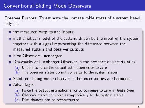
Observer of Utkin (reduced order SM observer)
Consider a nominal linear system
x(t) = Ax(t) + Bu(t) (1)
y(t) = Cx(t) (2)
Assume C has full row rank
Necessary and sufficient condition: (A,C ) is observable
Observability condition will be assumed to hold.
5

Outline
1 Conventional Sliding Mode ObserversA Simple Sliding Mode ObserverLTI systems with unknown inputs without need of differentiationWalcot-Zak Observes
6
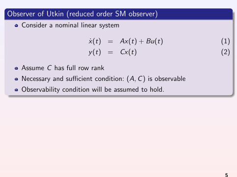
Coordinate transformation x 7→ z = Tc x
Tc =
[C⊥
C
](3)
where Nc ∈ Rn×(n−p) spans the null-space of C .
By construction det(Tc ) 6= 0
Applying the change of coordinates
TcAT−1c =
[A11 A12
A21 A22
], Tc B =
[B1
B2
], CT−1
c =[
0 Ip](4)
where A11 ∈ R(n−p)×(n−p) and B1 ∈ R(n−p)×q.
z1(t) = A11z1(t) + A12z2(t) + B1u, z2(t) = A21z1(t) + A22z2(t) + B2u
7
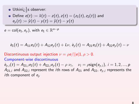
Utkinı¿ 12 s observer:
Define e(t) := x(t)− z(t), z(t) = (z1(t), z2(t)) andey (t) := y(t)− y(t) = y(t)− y(t)
e = col(e1, ey ), with e1 ∈ Rn−p
e1(t) = A11e1(t) + A12ey (t) + Lν, ey (t) = A21e1(t) + A22ey (t)− ν
Discontinuous output injection ν = ρe/||e|1, ρ > 0.Component-wise discontinuousey ,i (t) = A21,i e1(t) + A22,i ey (t)− ρ νi , νi = ρsign(ey ,i ), i = 1, 2, ..., pA21,i and A22,i represent the ith rows of A21 and A22, ey ,i represents theith component of ey
8

ν is designed to be discontinuous with respect to the sliding surfaceS = {e : Ce = 0} to force the trajectories of e(t) onto S in finitetime.
Gain Gn
Gn =
[L−Ip
](5)
where L ∈ R(n−p)×p represents the design freedom.
9
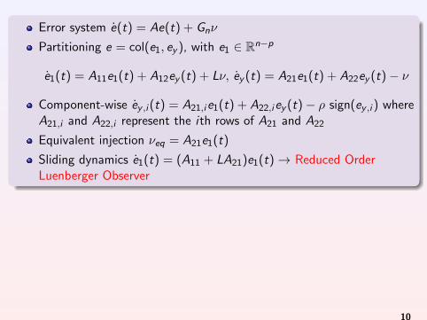
Error system e(t) = Ae(t) + Gnν
Partitioning e = col(e1, ey ), with e1 ∈ Rn−p
e1(t) = A11e1(t) + A12ey (t) + Lν, ey (t) = A21e1(t) + A22ey (t)− ν
Component-wise ey ,i (t) = A21,i e1(t) + A22,i ey (t)− ρ sign(ey ,i ) whereA21,i and A22,i represent the ith rows of A21 and A22
Equivalent injection νeq = A21e1(t)
Sliding dynamics e1(t) = (A11 + LA21)e1(t)→ Reduced OrderLuenberger Observer
10
Outline
1 Conventional Sliding Mode ObserversA Simple Sliding Mode ObserverLTI systems with unknown inputs without need of differentiationWalcot-Zak Observes
11
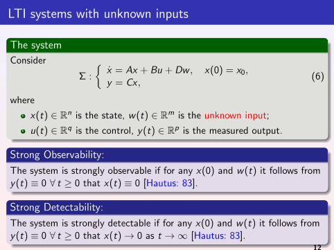
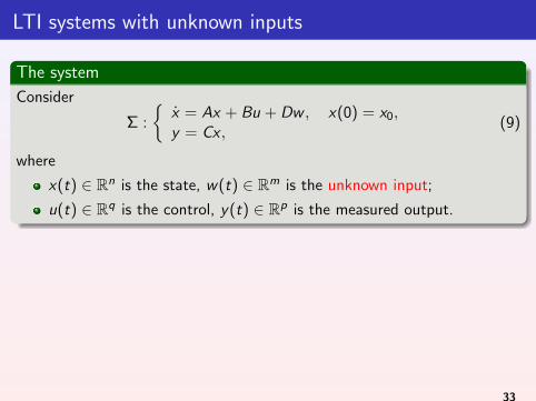
LTI systems with unknown inputs
The system
Consider
Σ :
{x = Ax + Bu + Dw , x(0) = x0,y = Cx ,
(6)
where
x(t) ∈ Rn is the state, w(t) ∈ Rm is the unknown input;
u(t) ∈ Rq is the control, y(t) ∈ Rp is the measured output.
Strong Observability:
The system is strongly observable if for any x(0) and w(t) it follows fromy(t) ≡ 0 ∀ t ≥ 0 that x(t) ≡ 0 [Hautus: 83].
Strong Detectability:
The system is strongly detectable if for any x(0) and w(t) it follows fromy(t) ≡ 0 ∀ t ≥ 0 that x(t)→ 0 as t →∞ [Hautus: 83].
12
LTI systems with unknown inputs
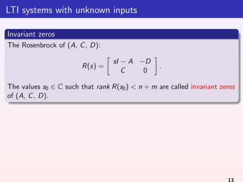
Invariant zeros
The Rosenbrock of (A, C , D):
R(s) =
[sI − A −D
C 0
].
The values s0 ∈ C such that rank R(s0) < n + m are called invariant zerosof (A, C , D).
13
Outline
1 Conventional Sliding Mode ObserversA Simple Sliding Mode ObserverLTI systems with unknown inputs without need of differentiationWalcot-Zak Observes
14
LTI systems with unknown inputs
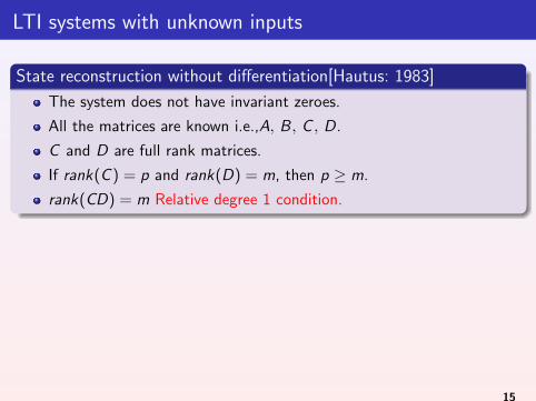
State reconstruction without differentiation[Hautus: 1983]
The system does not have invariant zeroes.
All the matrices are known i.e.,A, B, C , D.
C and D are full rank matrices.
If rank(C ) = p and rank(D) = m, then p ≥ m.
rank(CD) = m Relative degree 1 condition.
15

State Estimation and Unknown Inputs Reconstruction
Walcot-Zak Observes: Canonical form
dy⊥/dtdy1/dtdy2/dt
=
A11 A12 A13
A21 A22 A23
A31 A32 A33
y⊥
y1
y2
+ Bu +
00
w(t)
y1 non contaminated outputs,y2 contaminated outputs,y⊥ unmeasured states
The pair
(A11 A12
A21 A22
), (0, Ip−m) is observable
y⊥ can be obsevred with Luenberger or Utkin SM observer
Unknown Inputs can be reconstructed from Equivalent OutputsInjection ν = ρe2/||e2||, ρ > 0
16

This article has been accepted for inclusion in a future issue of this journal. Content is final as presented, with the exception of pagination.
FERREIRA et al.: ROBUST CONTROL WITH EXACT UNCERTAINTIES COMPENSATION 7
Fig. 4. Precision of [rad] using OISMC applying a (left) first-orderHOSM differentiator and a (right) second-order HOSM differentiator.
• two robust output feedback control strategies were com-pared:— continuous compensation control based on the es-
timated states and the compensation of identifiedunknown inputs (EOFS);
— output integral sliding mode control based on estimatedstates (OISMC).
• a methodology is suggested for the selection of an ap-propriate controller based on the comparison of both con-trol strategies considering the accuracy of observation andidentification algorithms as well as the actuator time con-stant;
• the proposed methodology is experimentally validated inan inverted rotary pendulum system.
REFERENCES
[1] V. I. Utkin, Sliding Modes in Control and Optimization. Berlin, Ger-many: Springer Verlag, 1992.
[2] V. I. Utkin, J. Guldner, and J. Shi, Sliding Modes in ElectromechanicalSystems. London, U.K.: Taylor and Francis, 1999.
[3] S. Laghrouche, F. Plestan, and A. Glumineau, “Higher order slidingmode control based on integral sliding mode,” Automatica, vol. 43, pp.531–537, 2007.
[4] L. Fridman, “Singularly perturbed analysis of chattering in relaycontrol systems,” IEEE Trans. Autom. Control, vol. 47, no. 12, pp.2079–2084, Dec. 2002.
[5] J. Alvarez, Y. Orlov, and L. Acho, “An invariance principle for discon-tinuous dynamic systems with application to a coulomb friction oscil-lator,” J. Dyn. Syst., Measure. Control, vol. 122, pp. 123–126, 2000.
[6] J. Barbot, M. Djemai, and T. Boukhobza, “Sliding mode observers,”in Sliding Mode Control in Engineering, W. Perruquetti and J. Barbot,Eds. New York: Marcel Dekker, 2002, pp. 103–130.
[7] I. Boiko, Discontinuous Control Systems: Frequency-Domain Analysisand Design. Boston, MA: Birkhäuser, 2009.
[8] C. Edwards and S. Spurgeon, Sliding Mode Control. London, U.K.:Taylor and Francis, 1998.
[9] Y. B. Shtessel, I. Shkolnikov, and A. Levant, “Smooth second-ordersliding modes: Missile guidance application,” Automatica, vol. 43, pp.1470–1476, 2007.
[10] W. Chen and M. Saif, “Actuator fault diagnosis for uncertainlinear systems using a high-order sliding-mode robust differentiator(HOSMRD),” Int. J. Rob. Nonlinear Control, vol. 18, pp. 413–426,2008.
[11] J. Barbot and T. Floquet, “A canonical form for the design of unknowninputs sliding mode observers,” in Advances in Variable Structure andSliding Mode Control, C. Edwards, E. Fossas-Colet, and L. Fridman,Eds. Berlin, Germany: Springer, 2006, vol. 334, pp. 103–130.
[12] A. Pisano and E. Usai, “Globally convergent real-time differentiationvia second order sliding modes,” Int. J. Control, vol. 38, pp. 833–844,2007.
[13] L. Fridman, A. Levant, and J. Davila, “Observation and identificationvia high-order sliding modes,” in Modern Sliding Mode ControlTheory New Perspectives and Applications, G. Bartolini, L. Fridman,A. Pisano, and E. Usai, Eds. Berlin, Germany: Springer Verlag,2008, pp. 293–320.
[14] F. Bejarano, L. Fridman, and A. Poznyak, “Exact state estima-tion for linear systems with unknown inputs based on hierarchicalsuper-twisting algorithm,” Int. J. Rob. Nonlinear Control, vol. 17, pp.1734–1753, 2007.
[15] A. Levant, “Higher-order sliding modes, differentiation and output-feedback control,” Int. J. Control, vol. 76, pp. 924–941, 2003.
[16] M. L. J. Hautus, “Strong detectability and observerss,” Linear Algebraand Its Applications, vol. 50, pp. 353–368, 1983.
[17] B. P. Molinari, “A strong controllability and observability in linearmultivariable control,” IEEE Trans. Autom. Control, vol. 21, no. 5, pp.761–764, Oct. 1976.
[18] M. Angulo and A. Levant, “On robust output based finite-time controlof systems using s,” in Proc. IFAC Conf. Anal. Des. Hy-brid Syst. (AHDS), 2009, pp. 222–227.
[19] A. N. Kolmogorov, “On inequalities between upper bounds of consecu-tive derivatives of an arbitrary function defined on an infinite interval,”(in Russian) Amer. Math. Soc. Transl. 2, pp. 233–242, 1962.
[20] A. Levant, “Robust exact differentiation via sliding mode technique,”Int. J. Control, vol. 34, pp. 379–384, 1998.
[21] B. Drazenovic, “The invariance conditions in variable structure sys-tems,” Automatica, vol. 5, pp. 287–295, 1969.
Alejandra Ferreira was born in Mexico in 1976.She received the B.Sc. degree from National Au-tonomous University of Mexico (UNAM), MexicoCity, Mexico, in 2004, where she is pursuing thePh.D. degree in automatic control.
In 2000–2005, she was with the InstrumentationDepartment, Institute of Astronomy, UNAM. Herprofessional interests include electronics design,observation, and identification of linear systems,sliding mode control, and its applications.
Francisco Javier Bejarano received the Masterand Doctor degrees in automatic control from theCINVESTAV-IPN, Mexico City, Mexico, in 2003and 2006, under the direction of Prof. A. Poznyakand Dr. L. Fridman.
He stayed one year at the ENSEA, France, and twoyears at UNAM, Mexico with respective posdoctoralpositions. He has published nine papers in interna-tional journals.
Leonid M. Fridman (M’98) received the M.S. de-gree in mathematics from Kuibyshev State Univer-sity, Samara, Russia, in 1976, the Ph.D. degree in ap-plied mathematics from the Institute of Control Sci-ence, Moscow, Russia, in 1988, and the Dr.Sci. de-gree in control science from Moscow State Universityof Mathematics and Electronics, Moscow, Russia, in1998.
From 1976 to 1999, he was with the Departmentof Mathematics, Samara State Architecture and CivilEngineering Academy. From 2000 to 2002, he was
with the Department of Postgraduate Study and Investigations at the ChihuahuaInstitute of Technology, Chihuahua, Mexico. In 2002, he joined the Departmentof Control, Division of Electrical Engineering of Engineering Faculty, NationalAutonomous University of Mexico (UNAM), México. He is an Editor of threebooks and five special issues on sliding mode control. He has published over200 technical papers. His research interests include variable structure systemsand singular perturbations.
Dr. Fridman is an Associate Editor of the International Journal of System Sci-ence and Conference Editorial Board of IEEE Control Systems Society, Memberof TC on Variable Structure Systems and Sliding mode control of IEEE ControlSystems Society.
Francisco Bejarano Jorge Davila Alejandra Ferreira Marco Tulio Angulo
Emmanuel Cruz Hector Rıos Rosalba Galvan Alejandro Apaza
17
Outline
1 Conventional Sliding Mode Observers
2 Higher Order Sliding Mode ObserversStrong Observability - Invariant Zeros - Relative DegreeRelation of concepts for SUISO SystemsMethodology: SM based differentiators
3 Cascaded HOSM Observers for Linear systems with unknown inputs
4 Super-twisting based Observers for Mechanical Systems
5 HOSM based Observers for Nonlinear Systems
6 Output-feedback finite-time stabilization of disturbed LTI systems
7 Unknown input identification
8 Parameter Identification
9 Output-based stabilization of disturbed systems
10 Switched Systems
11 Fault detection
18

Outline
2 Higher Order Sliding Mode ObserversStrong Observability - Invariant Zeros - Relative DegreeRelation of concepts for SUISO SystemsMethodology: SM based differentiators
19
Need of differentiation
Mechanical system
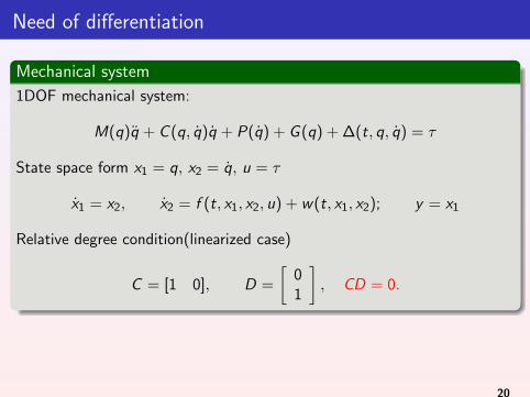
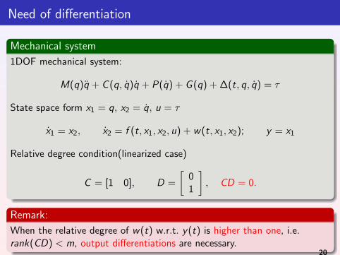
1DOF mechanical system:
M(q)q + C (q, q)q + P(q) + G (q) + ∆(t, q, q) = τ
State space form x1 = q, x2 = q, u = τ
x1 = x2, x2 = f (t, x1, x2, u) + w(t, x1, x2); y = x1
Relative degree condition(linearized case)
C = [1 0], D =
[01
], CD = 0.
Remark:
When the relative degree of w(t) w.r.t. y(t) is higher than one, i.e.rank(CD) < m, output differentiations are necessary.
20
Need of differentiation
Mechanical system
1DOF mechanical system:
M(q)q + C (q, q)q + P(q) + G (q) + ∆(t, q, q) = τ
State space form x1 = q, x2 = q, u = τ
x1 = x2, x2 = f (t, x1, x2, u) + w(t, x1, x2); y = x1
Relative degree condition(linearized case)
C = [1 0], D =
[01
], CD = 0.
Remark:
When the relative degree of w(t) w.r.t. y(t) is higher than one, i.e.rank(CD) < m, output differentiations are necessary.
20

Outline
2 Higher Order Sliding Mode ObserversStrong Observability - Invariant Zeros - Relative DegreeRelation of concepts for SUISO SystemsMethodology: SM based differentiators
21
Single Unknown Input- Single Output Case
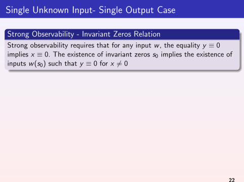
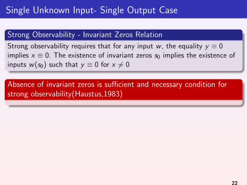
Strong Observability - Invariant Zeros Relation
Strong observability requires that for any input w , the equality y ≡ 0implies x ≡ 0. The existence of invariant zeros s0 implies the existence ofinputs w(s0) such that y ≡ 0 for x 6= 0
Absence of invariant zeros is sufficient and necessary condition forstrong observability(Haustus,1983)
22
Single Unknown Input- Single Output Case
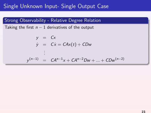
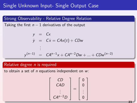
Strong Observability - Relative Degree Relation
Taking the first n − 1 derivatives of the output
y = Cx
y = C x = CAx(t) + CDw...
y (n−1) = CAn−1x + CAn−2Dw + ...+ CDw (n−2)
Relative degree n is required
to obtain a set of n equations independent on w :CD
CAD...
CAn−2D
=
00...0
23
Single Unknown Input- Single Output Case
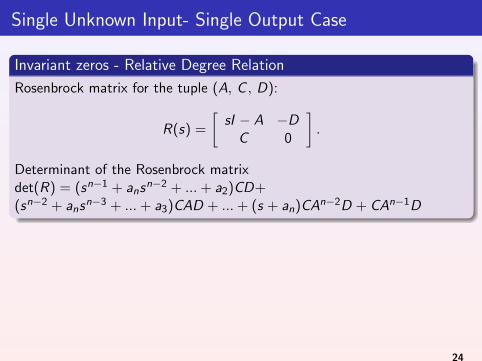
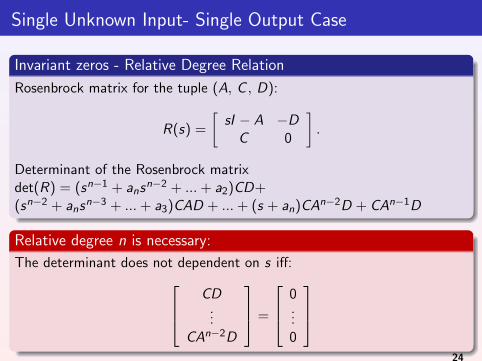
Invariant zeros - Relative Degree Relation
Rosenbrock matrix for the tuple (A, C , D):
R(s) =
[sI − A −D
C 0
].
Determinant of the Rosenbrock matrixdet(R) = (sn−1 + ansn−2 + ...+ a2)CD+(sn−2 + ansn−3 + ...+ a3)CAD + ...+ (s + an)CAn−2D + CAn−1D
Relative degree n is necessary:
The determinant does not dependent on s iff: CD...
CAn−2D
=
0...0
24
Single Unknown Input- Single Output Case
Invariant zeros - Relative Degree Relation
Rosenbrock matrix for the tuple (A, C , D):
R(s) =
[sI − A −D
C 0
].
Determinant of the Rosenbrock matrixdet(R) = (sn−1 + ansn−2 + ...+ a2)CD+(sn−2 + ansn−3 + ...+ a3)CAD + ...+ (s + an)CAn−2D + CAn−1D
Relative degree n is necessary:
The determinant does not dependent on s iff: CD...
CAn−2D
=
0...0
24

Outline
2 Higher Order Sliding Mode ObserversStrong Observability - Invariant Zeros - Relative DegreeRelation of concepts for SUISO SystemsMethodology: SM based differentiators
25
Differentiation Problem
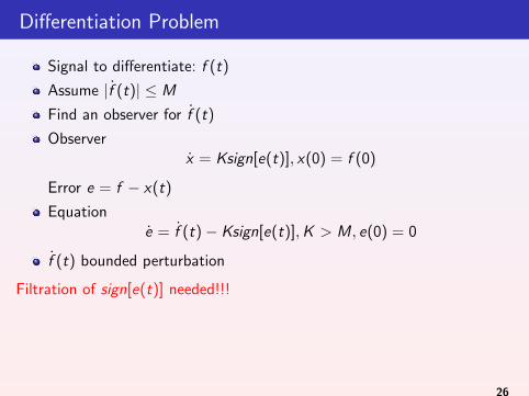
Signal to differentiate: f (t)
Assume |f (t)| ≤ M
Find an observer for f (t)
Observerx = Ksign[e(t)], x(0) = f (0)
Error e = f − x(t)
Equatione = f (t)− Ksign[e(t)],K > M, e(0) = 0
f (t) bounded perturbation
Filtration of sign[e(t)] needed!!!
26
Robust Exact Differentiation Problem
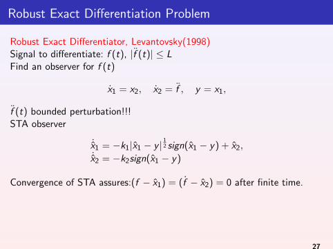
Robust Exact Differentiator, Levantovsky(1998)Signal to differentiate: f (t), |f (t)| ≤ LFind an observer for f (t)
x1 = x2, x2 = f , y = x1,
f (t) bounded perturbation!!!STA observer
˙x1 = −k1|x1 − y |12 sign(x1 − y) + x2,
˙x2 = −k2sign(x1 − y)
Convergence of STA assures:(f − x1) = (f − x2) = 0 after finite time.
27
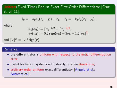
Uniform(Fixed-Time) Robust Exact First-Order Differentiator [Cruzet. al. 11].
z0 = −k1φ1(z0 − yj ) + z1, z1 = −k2φ2(z0 − yj ),
whereφ1(σ0) := dσ0c1/2 + dσ0c3/2,φ2(σ0) := 0,5 sign(σ0) + 2σ0 + 1,5dσ0c2.
and dvcp := |v |p sign(v).
Remarks.
the differentiator is uniform with respect to the initial differentiationerror;
useful for hybrid systems with strictly positive dwell-time;
arbitrary order uniform exact differentiator [Angulo et al.:Automatica].
28
3
and C1, C2, C3, and C4 are positive constants independent of theinitial conditions.
Proof: Appendix B.Since the high-degree terms of the URED are stronger than the
low-degree ones far from the origin, they are responsible for a fasterconvergence, and provide for the uniform convergence to a compactset �c
" containing the origin, as shown in Proposition 4. On the otherhand, Proposition 3 ensures the exact convergence of system (3) tothe origin, despite of the bounded perturbation
���f0 (t)��� < L, a fact
that is due to the low-degree terms, which are stronger than the high-degree ones in a neighborhood of the origin. Both Propositions 3 and4 together guarantee that the differentiator error (3) is uniformly exactconvergent, for f0 bounded, so that the convergence time of everytrajectory can be bounded by the same constant.
IV. CONVERGENCE TIME ESTIMATION
Once µ > 0 and the gains (k1, k2) have been selected, accordingto Theorem 2, (9) provides a convergence time estimation for thedifferentiator, that grows unboundedly with the norm of the initialdifferentiator error. However, (11) shows that any trajectory of thesame algorithm converges uniformly to the level set �c
", i.e. ina time bounded by the same constant, independent of the initialcondition. Combining both time estimations, an upper bound T forthe convergence time of any trajectory of (3) is given by
T 4�12max {P}
✏⌘
12 + 12 (2C2)
76
✓1
"
◆ 16
, (12)
where " � C1
⇣2C3 + 2
pC4 + C2
3
⌘3
, and the values ofC1, · · · , C4, ✏ and P are calculated as described in Appendices Aand B. Moreover, the value of ⌘ is selected, such that ⇤2," ⇢ ⌦1,⌘ ,where ⇤2," = {� | V2 (�) = "} is a level surface of V2 (�), and⌦1,⌘ = {� | V1 (�) ⌘} is a level set of V1 (�). ⇤2," ⇢ ⌦1,⌘ canalways be satisfied choosing ⌘ large enough.
An appropriate value of ⌘ can be calculated in the following form:
Choose ! >⇣
1C1
"⌘ 1
3 , so that the homogeneous ball Bh,! =n� | k�kr,p !
o� ⇤2,", where k·kr,p is an homogeneous norm
defined in Appendix B. Now, a value ⌫ has to be found, such thatB⌫ =
�� | k⇣k2 ⌫
� Bh,! , where k⇣k2
2 = |�0| + 2µ |�0|2 +
µ2 |�0|3 + �21 . This can be calculated by finding the maximum
value of k⇣k2 on the boundary of Bh,! . By simple calculus forthis maximum, k⇣k2
2 max = max�⇢�|�0|1
�, ⇢�|�0|2
� , where
⇢ (|�0|) = (µ |�0| + 1)2 |�0| +⇣!
27 � |�0|
72
⌘ 67 , |�0|1 = !
449 , and
|�0|2 is the only positive real root of
⇣!
27 � |�0|
72
⌘=
|�0|
52
(µ |�0| + 1)�µ |�0| + 1
3
�!7
.
Finally, selecting ⌫ > k⇣k2 max the required value of ⌘ is given by⌘ = �max {P} ⌫2.
Remark 5: Note from (12) that the prescribed time of the UREDis a constant, and it can be made arbitrarily small selecting the gainsk1 and k2 properly.
V. SIMULATION EXAMPLE
We compare the URED with Levant’s robust differentiator [5].For the simulation a value of µ = 1 has been set for the UREDand µ = 0 for Levant’s differentiator. The base signal to bedifferentiated is f0 (t) = 5t + sin t with two different noise terms:v1 (t) = 0.01 cos 10t, and v2 (t) = 0.001 cos 30t. With L = 2.5appropriate values for the gains are k1 = 2
p3, k2 = 6 (see
(4)) and two initial conditions for the output signal z(0) = 0 andz(0) = [10 , 0]T are taken. The results are shown in the Fig. 1.Both differentiators have robust and exact convergence. However,
Fig. 1. The URED (continuous line) and Levant’s robust exact differentiator[5] (dotted line)
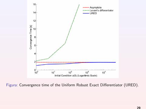
as shown in Fig. 2, the convergence time of Levant’s differentiator[5] grows unboundedly with the norm of the initial condition, whilethe convergence time of the URED is asymptotically bounded bya constant for growing initial condition’s norm. This prescribedconvergence time can be estimated by the expression (12).1) Selecting (see Appendix) � = 1.22228, we have �m = 2.14039,
Fig. 2. Convergence time of both differentiators by growing initial conditionnorm for f(t) = 5t + sin t + 0.01 cos 10t.
�M = 0.361173, ⇠ = 2.74119, C1 = 0.398254, C2 = 3.68254,C3 = 22.1792, C4 = 20.4383 and, consequently, " = 286752 andT2 (") = 15.1811.2) Find P = P T > 0 and ✏ > 0 such that (6) is satisfied. Thishappens for
A =
�3.4641 1
�6 0
�, P =
10.4315 �2.7068�2.7068 2.0680
�,
Limited circulation. For review only
Preprint submitted to IEEE Transactions on Automatic Control. Received: June 14, 2011 07:49:19 PST
Figura: Convergence time of the Uniform Robust Exact Differentiator (URED).
29
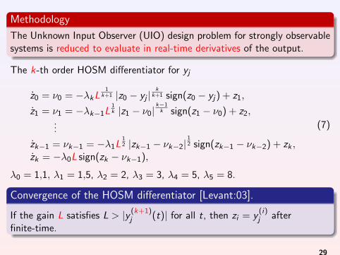
Methodology
The Unknown Input Observer (UIO) design problem for strongly observablesystems is reduced to evaluate in real-time derivatives of the output.
The k-th order HOSM differentiator for yj
z0 = ν0 = −λk L1
k+1 |z0 − yj |k
k+1 sign(z0 − yj ) + z1,
z1 = ν1 = −λk−1L1k |z1 − ν0|
k−1k sign(z1 − ν0) + z2,
...
zk−1 = νk−1 = −λ1L12 |zk−1 − νk−2|
12 sign(zk−1 − νk−2) + zk ,
zk = −λ0L sign(zk − νk−1),
(7)
λ0 = 1,1, λ1 = 1,5, λ2 = 2, λ3 = 3, λ4 = 5, λ5 = 8.
Convergence of the HOSM differentiator [Levant:03].
If the gain L satisfies L > |y (k+1)j (t)| for all t, then zi = y
(i)j after
finite-time.
29
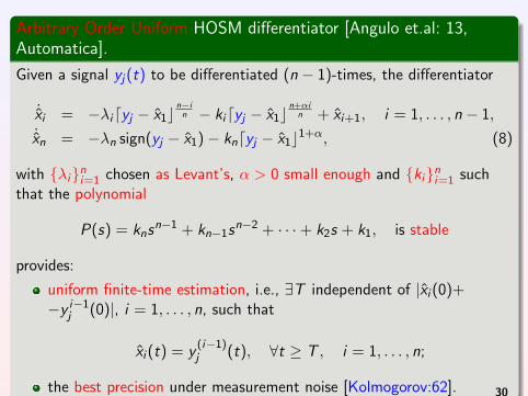
Arbitrary Order Uniform HOSM differentiator [Angulo et.al: 13,Automatica].
Given a signal yj (t) to be differentiated (n − 1)-times, the differentiator
˙xi = −λidyj − x1cn−i
n − kidyj − x1cn+αi
n + xi+1, i = 1, . . . , n − 1,
˙xn = −λn sign(yj − x1)− kndyj − x1c1+α, (8)
with {λi}ni=1 chosen as Levant’s, α > 0 small enough and {ki}n
i=1 suchthat the polynomial
P(s) = knsn−1 + kn−1sn−2 + · · ·+ k2s + k1, is stable
provides:
uniform finite-time estimation, i.e., ∃T independent of |xi (0)+−y i−1
j (0)|, i = 1, . . . , n, such that
xi (t) = y(i−1)j (t), ∀t ≥ T , i = 1, . . . , n;
the best precision under measurement noise [Kolmogorov:62]. 30
Outline
1 Conventional Sliding Mode Observers
2 Higher Order Sliding Mode Observers
3 Cascaded HOSM Observers for Linear systems with unknown inputsCascaded HOSM Observers for LTI systems with unknown inputsCascaded HOSM Observers for LTV systems with Unknown inputsCascaded Observers for strong detectable LTI systems with unknowninputsCascaded Functional HOSM Observers for linear systems
4 Super-twisting based Observers for Mechanical Systems
5 HOSM based Observers for Nonlinear Systems
6 Output-feedback finite-time stabilization of disturbed LTI systems
7 Unknown input identification
8 Parameter Identification
9 Output-based stabilization of disturbed systems
10 Switched Systems
11 Fault detection
31
Outline
3 Cascaded HOSM Observers for Linear systems with unknown inputsCascaded HOSM Observers for LTI systems with unknown inputsCascaded HOSM Observers for LTV systems with Unknown inputsCascaded Observers for strong detectable LTI systems with unknowninputsCascaded Functional HOSM Observers for linear systems
32
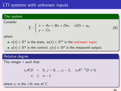
LTI systems with unknown inputs
The system
Consider
Σ :
{x = Ax + Bu + Dw , x(0) = x0,y = Cx ,
(9)
where
x(t) ∈ Rn is the state, w(t) ∈ Rm is the unknown input;
u(t) ∈ Rq is the control, y(t) ∈ Rp is the measured output.
Relative degree
The integer r such that
ci Aj D = 0, j = 0, ..., ri − 2, ci A
ri−1D 6= 0,
ri ≤ n − 1
where ci is the i-th row of C .
33
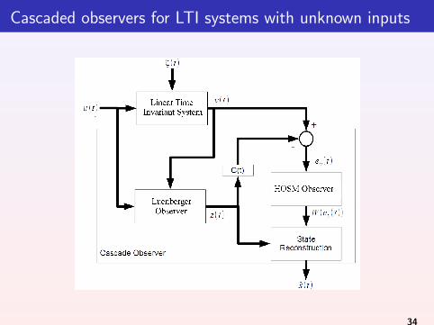
Cascaded observers for LTI systems with unknown inputs
34
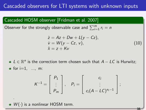
Cascaded observers for LTI systems with unknown inputs
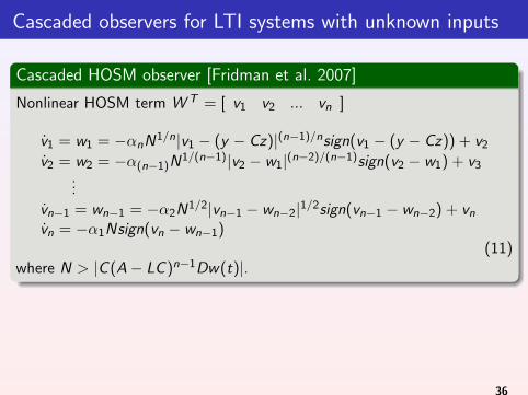
Cascaded HOSM observer [Fridman et al. 2007]
Observer for the strongly observable case and∑m
i=1 ri = n
z = Az + Dw + L(y − Cz),v = W (y − Cz , v),x = z + Kv
(10)
L ∈ Rn is the correction term chosen such that A− LC is Hurwitz;
for i=1, ..., m:
K−1 =
P1...
Pm
, Pi =
ci...
ci (A− LC )ni−1
;
.
W (·) is a nonlinear HOSM term.35
Cascaded observers for LTI systems with unknown inputs
Cascaded HOSM observer [Fridman et al. 2007]
Nonlinear HOSM term W T = [ v1 v2 ... vn ]
v1 = w1 = −αnN1/n|v1 − (y − Cz)|(n−1)/nsign(v1 − (y − Cz)) + v2
v2 = w2 = −α(n−1)N1/(n−1)|v2 − w1|(n−2)/(n−1)sign(v2 − w1) + v3...
vn−1 = wn−1 = −α2N1/2|vn−1 − wn−2|1/2sign(vn−1 − wn−2) + vn
vn = −α1Nsign(vn − wn−1)(11)
where N > |C (A− LC )n−1Dw(t)|.
36
Cascaded observers for LTI systems with unknown inputs
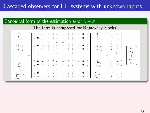
Canonical form of the estimation error x − z
The form is composed for Brunovsky blocks.
37
Cascaded observers for LTI systems with unknown inputs
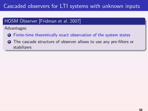
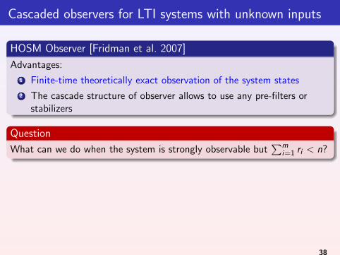
HOSM Observer [Fridman et al. 2007]
Advantages:
1 Finite-time theoretically exact observation of the system states
2 The cascade structure of observer allows to use any pre-filters orstabilizers
Question
What can we do when the system is strongly observable but∑m
i=1 ri < n?
38
Cascaded observers for LTI systems with unknown inputs
HOSM Observer [Fridman et al. 2007]
Advantages:
1 Finite-time theoretically exact observation of the system states
2 The cascade structure of observer allows to use any pre-filters orstabilizers
Question
What can we do when the system is strongly observable but∑m
i=1 ri < n?
38
Weakly unobservable subspace
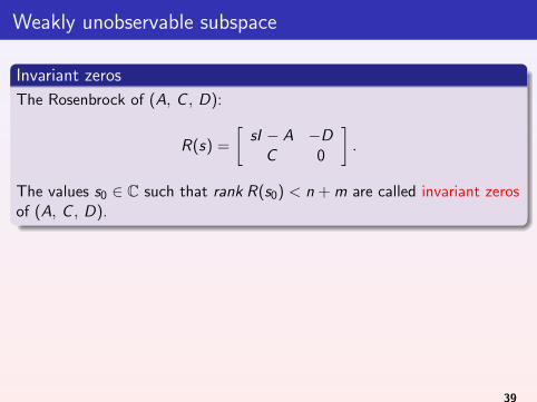
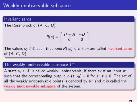
Invariant zeros
The Rosenbrock of (A, C , D):
R(s) =
[sI − A −D
C 0
].
The values s0 ∈ C such that rank R(s0) < n + m are called invariant zerosof (A, C , D).
The weakly unobservable subspace V∗
A state x0 ∈ X is called weakly unobservable, if there exist an input wsuch that the corresponding output yw (t, x0) = 0 for all t ≥ 0. The set ofall the weakly unobservable points is denoted by V∗ and it is called theweakly unobservable subspace of the system.
39
Weakly unobservable subspace
Invariant zeros
The Rosenbrock of (A, C , D):
R(s) =
[sI − A −D
C 0
].
The values s0 ∈ C such that rank R(s0) < n + m are called invariant zerosof (A, C , D).
The weakly unobservable subspace V∗
A state x0 ∈ X is called weakly unobservable, if there exist an input wsuch that the corresponding output yw (t, x0) = 0 for all t ≥ 0. The set ofall the weakly unobservable points is denoted by V∗ and it is called theweakly unobservable subspace of the system.
39
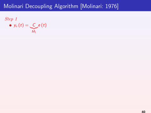
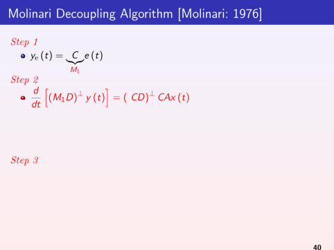
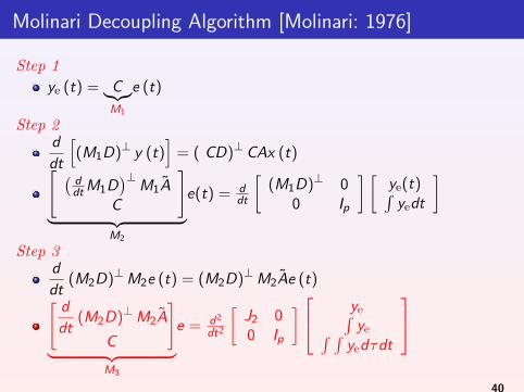
Molinari Decoupling Algorithm [Molinari: 1976]
Step 1
ye (t) = C︸︷︷︸M1
e (t)
Step 2
d
dt
[(M1D)⊥ y (t)
]= ( CD)⊥ CAx (t)[ (
ddt M1D
)⊥M1A
C
]︸ ︷︷ ︸
M2
e(t) = ddt
[(M1D)⊥ 0
0 Ip
] [ye(t)∫
yedt
]
Step 3
d
dt(M2D)⊥M2e (t) = (M2D)⊥M2Ae (t)[
d
dt(M2D)⊥M2A
C
]︸ ︷︷ ︸
M3
e = d2
dt2
[J2 00 Ip
] ye∫ye∫ ∫
yedτdt
40
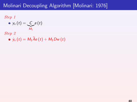
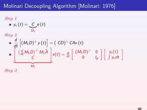
Molinari Decoupling Algorithm [Molinari: 1976]
Step 1
ye (t) = C︸︷︷︸M1
e (t)
Step 2
ye (t) = M1Ae (t) + M1Dw (t)
[ (ddt M1D
)⊥M1A
C
]︸ ︷︷ ︸
M2
e(t) = ddt
[(M1D)⊥ 0
0 Ip
] [ye(t)∫
yedt
]
Step 3
d
dt(M2D)⊥M2e (t) = (M2D)⊥M2Ae (t)[
d
dt(M2D)⊥M2A
C
]︸ ︷︷ ︸
M3
e = d2
dt2
[J2 00 Ip
] ye∫ye∫ ∫
yedτdt
40
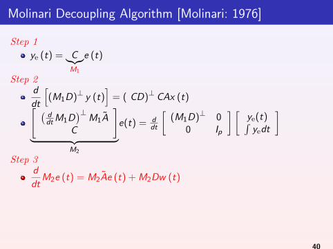
Molinari Decoupling Algorithm [Molinari: 1976]
Step 1
ye (t) = C︸︷︷︸M1
e (t)
Step 2d
dt
[(M1D)⊥ y (t)
]= ( CD)⊥ CAx (t)
[ (ddt M1D
)⊥M1A
C
]︸ ︷︷ ︸
M2
e(t) = ddt
[(M1D)⊥ 0
0 Ip
] [ye(t)∫
yedt
]
Step 3
d
dt(M2D)⊥M2e (t) = (M2D)⊥M2Ae (t)[
d
dt(M2D)⊥M2A
C
]︸ ︷︷ ︸
M3
e = d2
dt2
[J2 00 Ip
] ye∫ye∫ ∫
yedτdt
40
Molinari Decoupling Algorithm [Molinari: 1976]
Step 1
ye (t) = C︸︷︷︸M1
e (t)
Step 2d
dt
[(M1D)⊥ y (t)
]= ( CD)⊥ CAx (t)[ (
ddt M1D
)⊥M1A
C
]︸ ︷︷ ︸
M2
e(t) = ddt
[(M1D)⊥ 0
0 Ip
] [ye(t)∫
yedt
]
Step 3
d
dt(M2D)⊥M2e (t) = (M2D)⊥M2Ae (t)[
d
dt(M2D)⊥M2A
C
]︸ ︷︷ ︸
M3
e = d2
dt2
[J2 00 Ip
] ye∫ye∫ ∫
yedτdt
40
Molinari Decoupling Algorithm [Molinari: 1976]
Step 1
ye (t) = C︸︷︷︸M1
e (t)
Step 2d
dt
[(M1D)⊥ y (t)
]= ( CD)⊥ CAx (t)[ (
ddt M1D
)⊥M1A
C
]︸ ︷︷ ︸
M2
e(t) = ddt
[(M1D)⊥ 0
0 Ip
] [ye(t)∫
yedt
]
Step 3d
dtM2e (t) = M2Ae (t) + M2Dw (t)
[d
dt(M2D)⊥M2A
C
]︸ ︷︷ ︸
M3
e = d2
dt2
[J2 00 Ip
] ye∫ye∫ ∫
yedτdt
40
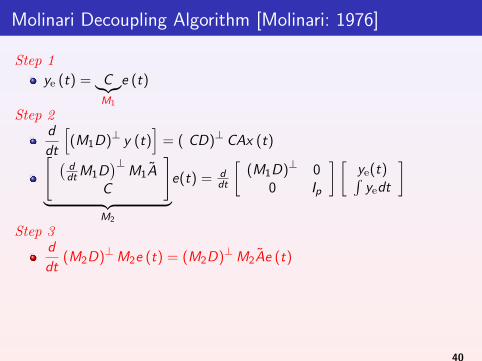
Molinari Decoupling Algorithm [Molinari: 1976]
Step 1
ye (t) = C︸︷︷︸M1
e (t)
Step 2d
dt
[(M1D)⊥ y (t)
]= ( CD)⊥ CAx (t)[ (
ddt M1D
)⊥M1A
C
]︸ ︷︷ ︸
M2
e(t) = ddt
[(M1D)⊥ 0
0 Ip
] [ye(t)∫
yedt
]
Step 3d
dt(M2D)⊥M2e (t) = (M2D)⊥M2Ae (t)
[d
dt(M2D)⊥M2A
C
]︸ ︷︷ ︸
M3
e = d2
dt2
[J2 00 Ip
] ye∫ye∫ ∫
yedτdt
40
Molinari Decoupling Algorithm [Molinari: 1976]
Step 1
ye (t) = C︸︷︷︸M1
e (t)
Step 2d
dt
[(M1D)⊥ y (t)
]= ( CD)⊥ CAx (t)[ (
ddt M1D
)⊥M1A
C
]︸ ︷︷ ︸
M2
e(t) = ddt
[(M1D)⊥ 0
0 Ip
] [ye(t)∫
yedt
]
Step 3d
dt(M2D)⊥M2e (t) = (M2D)⊥M2Ae (t)[
d
dt(M2D)⊥M2A
C
]︸ ︷︷ ︸
M3
e = d2
dt2
[J2 00 Ip
] ye∫ye∫ ∫
yedτdt
40
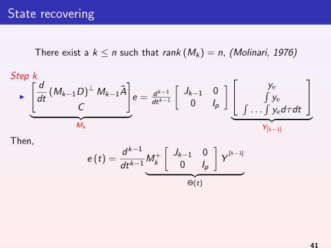
State recovering
There exist a k ≤ n such that rank (Mk ) = n, (Molinari, 1976)
Step k
I
[d
dt(Mk−1D)⊥Mk−1A
C
]︸ ︷︷ ︸
Mk
e = dk−1
dtk−1
[Jk−1 0
0 Ip
] ye∫ye∫
. . .∫
yedτdt
︸ ︷︷ ︸
Y[k−1]
Then,
e (t) =dk−1
dtk−1M+
k
[Jk−1 0
0 Ip
]Y
[k−1]
︸ ︷︷ ︸Θ(t)
41
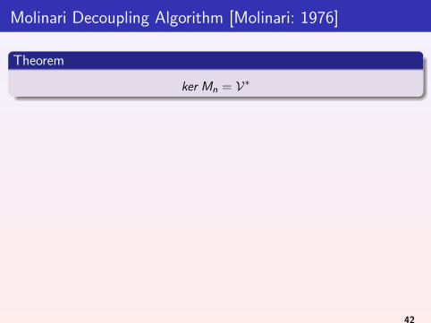
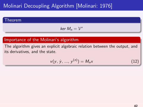
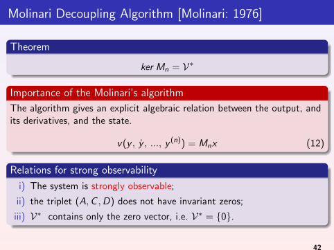
Molinari Decoupling Algorithm [Molinari: 1976]
Theorem
ker Mn = V∗
Importance of the Molinari’s algorithm
The algorithm gives an explicit algebraic relation between the output, andits derivatives, and the state.
v(y , y , ..., y (n)) = Mnx (12)
Relations for strong observability
i) The system is strongly observable;
ii) the triplet (A,C ,D) does not have invariant zeros;
iii) V∗ contains only the zero vector, i.e. V∗ = {0}.
42
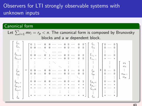
Observers for LTI strongly observable systems withunknown inputs
Canonical form
Let∑
i=1 mri = rp < n. The canonical form is composed by Brunovskyblocks and a w dependent block.
43
Cascaded observers for LTI strongly observable systemswith unknown inputs
Observer in [Fridman et al. 2007]
X The states are estimated exactly after finite time;
X The cascade structure of observer allows to use a pre-filter.
44
Outline
3 Cascaded HOSM Observers for Linear systems with unknown inputsCascaded HOSM Observers for LTI systems with unknown inputsCascaded HOSM Observers for LTV systems with Unknown inputsCascaded Observers for strong detectable LTI systems with unknowninputsCascaded Functional HOSM Observers for linear systems
45
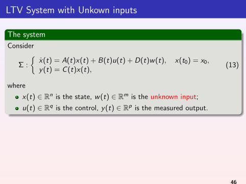
LTV System with Unkown inputs
The system
Consider
Σ :
{x(t) = A(t)x(t) + B(t)u(t) + D(t)w(t), x(t0) = x0,y(t) = C (t)x(t),
(13)
where
x(t) ∈ Rn is the state, w(t) ∈ Rm is the unknown input;
u(t) ∈ Rq is the control, y(t) ∈ Rp is the measured output.
46
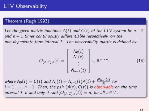
LTV Observability
Theorem (Rugh 1993)
Let the given matrix functions A(t) and C (t) of the LTV system be n − 2and n − 1 times continuously differentiable respectively, on thenon-degenerate time interval T . The observability matrix is defined by
O(A,C),n(t) =
N0(t)N1(t)
...Nn−1(t)
∈ Rpn×n, (14)
where N0(t) = C (t) and Ni (t) = Ni−1(t)A(t) +dNi−1(t)
dt fori = 1, . . . , n − 1. Then, the pair (A(t),C (t)) is observable on the timeinterval T if and only if rank(O(A,C),n(t)) = n, for all t ∈ T .
47
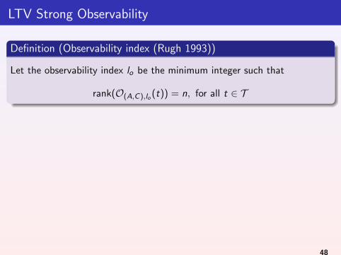
LTV Strong Observability
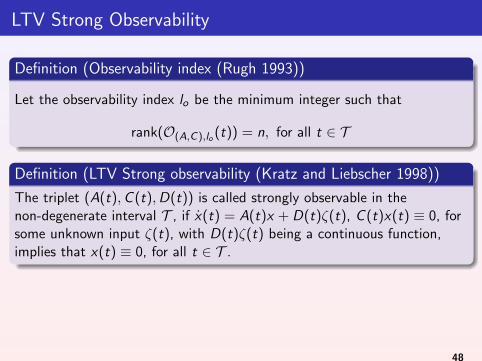
Definition (Observability index (Rugh 1993))
Let the observability index lo be the minimum integer such that
rank(O(A,C),lo (t)) = n, for all t ∈ T
Definition (LTV Strong observability (Kratz and Liebscher 1998))
The triplet (A(t),C (t),D(t)) is called strongly observable in thenon-degenerate interval T , if x(t) = A(t)x + D(t)ζ(t), C (t)x(t) ≡ 0, forsome unknown input ζ(t), with D(t)ζ(t) being a continuous function,implies that x(t) ≡ 0, for all t ∈ T .
48
LTV Strong Observability
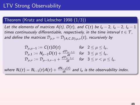
Theorem (Kratz and Liebscher 1998 (1/3))
Let the elements of matrices A(t), D(t), and C (t) be lo − 2, lo − 2, lo − 1times continuously differentiable, respectively, in the time interval t ∈ T ,and define the matrices Dµ,ν = D(A,C ,D),µ,ν(t), recursively by
Dµ,µ−1 := C (t)D(t) for 2 ≤ µ ≤ lo ,
Dµ,1 := Nµ−2D(t) +dDµ−1,1
dt for 3 ≤ µ ≤ lo ,
Dµ,ν := Dµ−1,ν−1 +dDµ−1,ν
dt for 3 ≤ ν < µ ≤ lo .
where Ni (t) = Ni−1(t)A(t) +dNi−1(t)
dt and lo is the observability index.
49
LTV Strong Observability
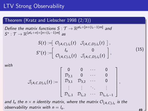
Theorem (Kratz and Liebscher 1998 (2/3))
Define the matrix functions S : T → Rplo×[n+(lo−1)m] andS∗ : T → R(plo +n)×[n+(lo−1)m] as
S(t) :=[O(A,C),lo (t) J(A,C ,D),lo (t)
],
S∗(t) :=
[In 0
O(A,C),lo (t) J(A,C ,D),lo (t)
],
(15)
with
J(A,C ,D),lo (t) :=
0 0 · · · 0D2,1 0 · · · 0D3,1 D3,2 · · · 0
......
. . ....
Dlo ,1 Dlo ,2 · · · Dlo ,lo−1
,and In the n × n identity matrix, where the matrix O(A,C),lo is theobservability matrix with n = lo .
49
LTV Strong Observability
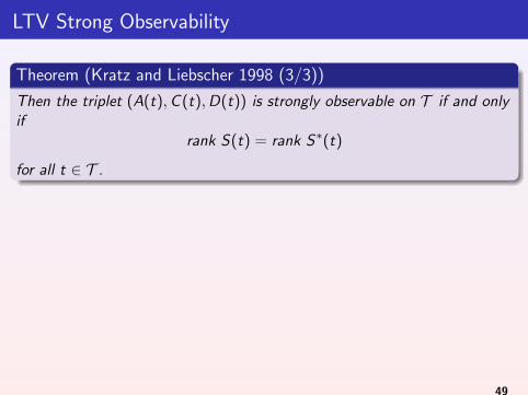
Theorem (Kratz and Liebscher 1998 (3/3))
Then the triplet (A(t),C (t),D(t)) is strongly observable on T if and onlyif
rank S(t) = rank S∗(t)
for all t ∈ T .
49
LTV Strong Observability: State reconstruction
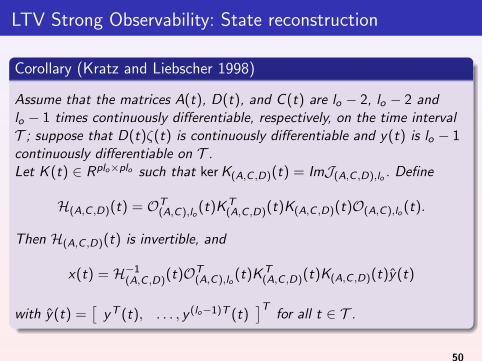
Corollary (Kratz and Liebscher 1998)
Assume that the matrices A(t), D(t), and C (t) are lo − 2, lo − 2 andlo − 1 times continuously differentiable, respectively, on the time intervalT ; suppose that D(t)ζ(t) is continuously differentiable and y(t) is lo − 1continuously differentiable on T .Let K (t) ∈ Rplo×plo such that ker K(A,C ,D)(t) = ImJ(A,C ,D),lo . Define
H(A,C ,D)(t) = OT(A,C),lo
(t)K T(A,C ,D)(t)K(A,C ,D)(t)O(A,C),lo (t).
Then H(A,C ,D)(t) is invertible, and
x(t) = H−1(A,C ,D)(t)OT
(A,C),lo(t)K T
(A,C ,D)(t)K(A,C ,D)(t)y(t)
with y(t) =[
y T (t), . . . , y (lo−1)T (t)]T
for all t ∈ T .
50
Cascaded observers for strongly observable LTV systems R.Galvan et al, 2017
Assumptions
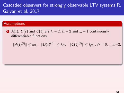
1 A(t), D(t) and C (t) are lo − 2, lo − 2 and lo − 1 continuouslydifferentiable functions,
‖A(t)(i)‖ ≤ ki1; ‖D(t)(i)‖ ≤ ki2; ‖C (t)(j)‖ ≤ kj3 ,∀i = 0, ..., n−2; j = 0, ..., lo−1,
2 ‖ζ(t)(i)‖ ≤ ζ+i , ∀i = 0, ..., n − 1
3 (A(t),D(t),C (t)) is strongly observable.
51
Cascaded observers for strongly observable LTV systems R.Galvan et al, 2017
Assumptions
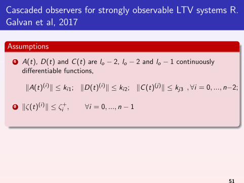
1 A(t), D(t) and C (t) are lo − 2, lo − 2 and lo − 1 continuouslydifferentiable functions,
‖A(t)(i)‖ ≤ ki1; ‖D(t)(i)‖ ≤ ki2; ‖C (t)(j)‖ ≤ kj3 ,∀i = 0, ..., n−2; j = 0, ..., lo−1,
2 ‖ζ(t)(i)‖ ≤ ζ+i , ∀i = 0, ..., n − 1
3 (A(t),D(t),C (t)) is strongly observable.
51
Cascaded observers for strongly observable LTV systems R.Galvan et al, 2017
Assumptions
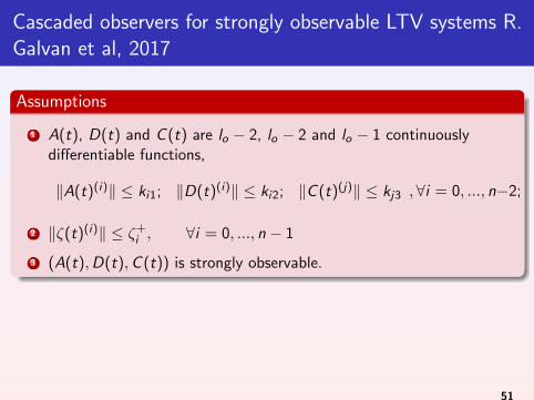
1 A(t), D(t) and C (t) are lo − 2, lo − 2 and lo − 1 continuouslydifferentiable functions,
‖A(t)(i)‖ ≤ ki1; ‖D(t)(i)‖ ≤ ki2; ‖C (t)(j)‖ ≤ kj3 ,∀i = 0, ..., n−2; j = 0, ..., lo−1,
2 ‖ζ(t)(i)‖ ≤ ζ+i , ∀i = 0, ..., n − 1
3 (A(t),D(t),C (t)) is strongly observable.
51
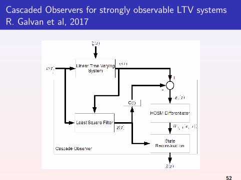
Cascaded Observers for strongly observable LTV systemsR. Galvan et al, 2017
52
Observers for strongly observable LTV systems R. Galvanet al, 2017
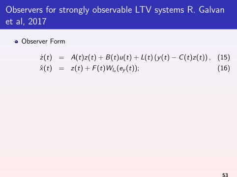
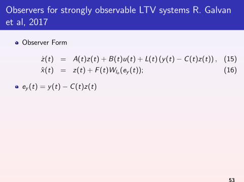
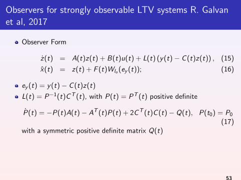
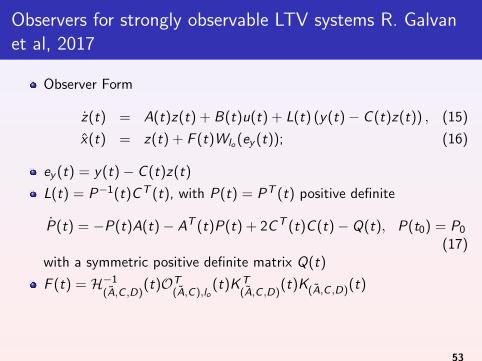
Observer Form
z(t) = A(t)z(t) + B(t)u(t) + L(t) (y(t)− C (t)z(t)) , (15)
x(t) = z(t) + F (t)Wlo (ey (t)); (16)
ey (t) = y(t)− C (t)z(t)
L(t) = P−1(t)C T (t), with P(t) = PT (t) positive definite
P(t) = −P(t)A(t)− AT (t)P(t) + 2C T (t)C (t)− Q(t), P(t0) = P0
(17)with a symmetric positive definite matrix Q(t)
F (t) = H−1(A,C ,D)
(t)OT(A,C),lo
(t)K T(A,C ,D)
(t)K(A,C ,D)(t)
53
Observers for strongly observable LTV systems R. Galvanet al, 2017
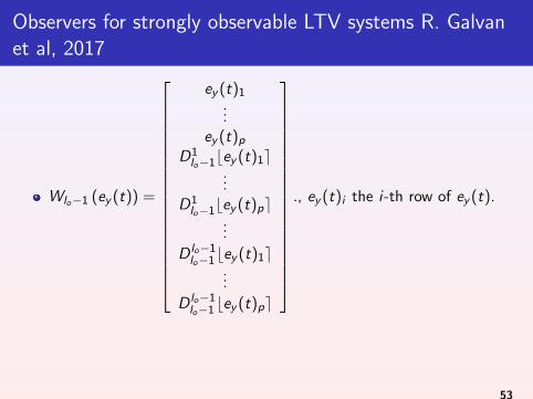
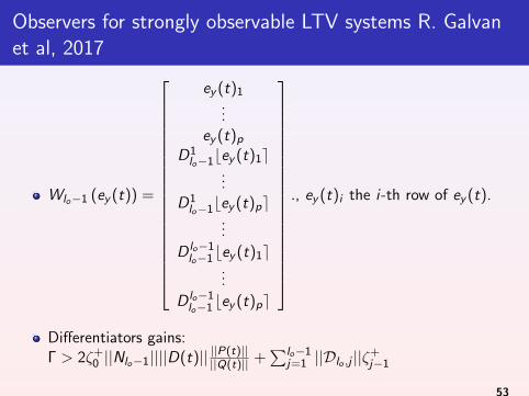
Wlo−1 (ey (t)) =
ey (t)1...
ey (t)p
D1lo−1bey (t)1e
...D1
lo−1bey (t)pe...
D lo−1lo−1bey (t)1e
...
D lo−1lo−1bey (t)pe
., ey (t)i the i-th row of ey (t).
53
Observers for strongly observable LTV systems R. Galvanet al, 2017
Wlo−1 (ey (t)) =
ey (t)1...
ey (t)p
D1lo−1bey (t)1e
...D1
lo−1bey (t)pe...
D lo−1lo−1bey (t)1e
...
D lo−1lo−1bey (t)pe
., ey (t)i the i-th row of ey (t).
Differentiators gains:Γ > 2ζ+
0 ||Nlo−1||||D(t)|| ||P(t)||||Q(t)|| +
∑lo−1j=1 ||Dlo ,j ||ζ+
j−1
53
Cascaded Observers for strongly observable LTV systemsR. Galvan et al, 2017
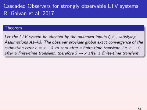
Theorem
Let the LTV system be affected by the unknown inputs ζ(t), satisfyingAssumptions A1-A3. The observer provides global exact convergence of theestimation error e = x − x to zero after a finite-time transient, i.e. e → 0after a finite-time transient, therefore x → x after a finite-time transient.
54
Observers for strongly observable LTV systems R. Galvanet al, 2017
Highlights
X The states are reconstructed exactly after finite time;
X Deterministic Least Square Filter is combined with a HOSMdifferentiator
X The LTV can be unstable
55
Observers for strongly observable LTV systems R. Galvanet al, 2017
Highlights
X The states are reconstructed exactly after finite time;
X Deterministic Least Square Filter is combined with a HOSMdifferentiator
X The LTV can be unstable
55
Observers for strongly observable LTV systems R. Galvanet al, 2017
Highlights
X The states are reconstructed exactly after finite time;
X Deterministic Least Square Filter is combined with a HOSMdifferentiator
X The LTV can be unstable
55
Outline
3 Cascaded HOSM Observers for Linear systems with unknown inputsCascaded HOSM Observers for LTI systems with unknown inputsCascaded HOSM Observers for LTV systems with Unknown inputsCascaded Observers for strong detectable LTI systems with unknowninputsCascaded Functional HOSM Observers for linear systems
56
Strong detectability
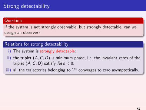
Question
If the system is not strongly observable, but strongly detectable, can wedesign an observer?
Relations for strong detectability
i) The system is strongly detectable;
ii) the triplet (A,C ,D) is minimum phase, i.e. the invariant zeros of thetriplet (A,C ,D) satisfy Re s < 0;
iii) all the trajectories belonging to V∗ converges to zero asymptotically.
57
Strong detectability
Question
If the system is not strongly observable, but strongly detectable, can wedesign an observer?
Relations for strong detectability
i) The system is strongly detectable;
ii) the triplet (A,C ,D) is minimum phase, i.e. the invariant zeros of thetriplet (A,C ,D) satisfy Re s < 0;
iii) all the trajectories belonging to V∗ converges to zero asymptotically.
57

State space
State space for LSUI
The state space is divided in strongly observable and the weaklyunobservable sub-spaces. But the weakly unobservable subspace containsthe systems unobservable subspace.
State space for systems with unknown inputs.
58

State space
State space for LSUI
The state space is divided in strongly observable and the weaklyunobservable sub-spaces. But the weakly unobservable subspace containsthe systems unobservable subspace.
State space for systems with unknown inputs.
58
Cascaded Observers for strongly detectable LTI systems
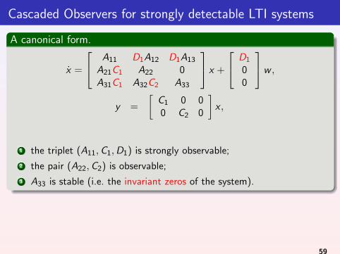
A canonical form.
x =
A11 D1A12 D1A13
A21C1 A22 0A31C1 A32C2 A33
x +
D1
00
w ,
y =
[C1 0 00 C2 0
]x ,
1 the triplet (A11,C1,D1) is strongly observable;
2 the pair (A22,C2) is observable;
3 A33 is stable (i.e. the invariant zeros of the system).
59
Cascaded Observers for strongly detectable LTI systems
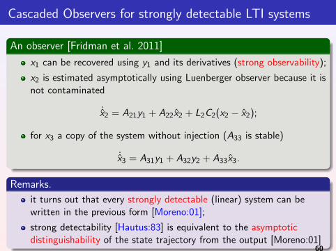
An observer [Fridman et al. 2011]
x1 can be recovered using y1 and its derivatives (strong observability);
x2 is estimated asymptotically using Luenberger observer because it isnot contaminated
˙x2 = A21y1 + A22x2 + L2C2(x2 − x2);
for x3 a copy of the system without injection (A33 is stable)
˙x3 = A31y1 + A32y2 + A33x3.
Remarks.
it turns out that every strongly detectable (linear) system can bewritten in the previous form [Moreno:01];
strong detectability [Hautus:83] is equivalent to the asymptoticdistinguishability of the state trajectory from the output [Moreno:01]
60

Question
What happens when the system is not strongly observable. Is still possibleto do something?
61
Outline
3 Cascaded HOSM Observers for Linear systems with unknown inputsCascaded HOSM Observers for LTI systems with unknown inputsCascaded HOSM Observers for LTV systems with Unknown inputsCascaded Observers for strong detectable LTI systems with unknowninputsCascaded Functional HOSM Observers for linear systems
62
Functional Unknown Input Observers
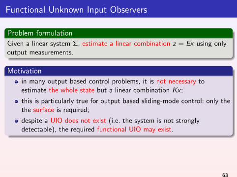
Problem formulation
Given a linear system Σ, estimate a linear combination z = Ex using onlyoutput measurements.
Motivation
in many output based control problems, it is not necessary toestimate the whole state but a linear combination Kx ;
this is particularly true for output based sliding-mode control: only thethe surface is required;
despite a UIO does not exist (i.e. the system is not stronglydetectable), the required functional UIO may exist.
63
Functional Unknown Input Observers
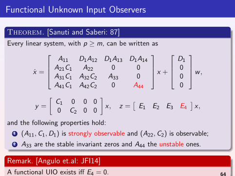
Theorem. [Sanuti and Saberi: 87]
Every linear system, with p ≥ m, can be written as
x =
A11 D1A12 D1A13 D1A14
A21C1 A22 0 0A31C1 A32C2 A33 0A41C1 A42C2 0 A44
x +
D1
000
w ,
y =
[C1 0 0 00 C2 0 0
]x , z =
[E1 E2 E3 E4
]x ,
and the following properties hold:
1 (A11,C1,D1) is strongly observable and (A22,C2) is observable;
2 A33 are the stable invariant zeros and A44 the unstable ones.
Remark. [Angulo et.al: JFI14]
A functional UIO exists iff E4 = 0. 64
Outline
1 Conventional Sliding Mode Observers
2 Higher Order Sliding Mode Observers
3 Cascaded HOSM Observers for Linear systems with unknown inputs
4 Super-twisting based Observers for Mechanical SystemsSuper-twisting based Observers for Mechanical systems a-prioribounded Coriolis term
5 HOSM based Observers for Nonlinear Systems
6 Output-feedback finite-time stabilization of disturbed LTI systems
7 Unknown input identification
8 Parameter Identification
9 Output-based stabilization of disturbed systems
10 Switched Systems
11 Fault detection
65

Outline
4 Super-twisting based Observers for Mechanical SystemsSuper-twisting based Observers for Mechanical systems a-prioribounded Coriolis term
66
Super-twisting based Observers for Mechanical systemswith a-priori bounded Coriolis term
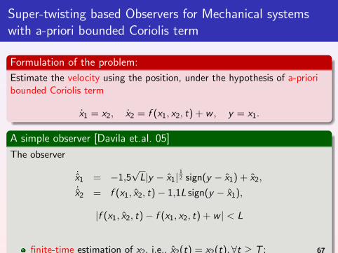
Formulation of the problem:
Estimate the velocity using the position, under the hypothesis of a-prioribounded Coriolis term
x1 = x2, x2 = f (x1, x2, t) + w , y = x1.
A simple observer [Davila et.al. 05]
The observer
˙x1 = −1,5√
L|y − x1|12 sign(y − x1) + x2,
˙x2 = f (x1, x2, t)− 1,1L sign(y − x1),
|f (x1, x2, t)− f (x1, x2, t) + w | < L
finite-time estimation of x2, i.e., x2(t) = x2(t),∀t ≥ T ;
the best precision in the sense of [Kolmogorov:62].
67

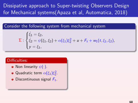
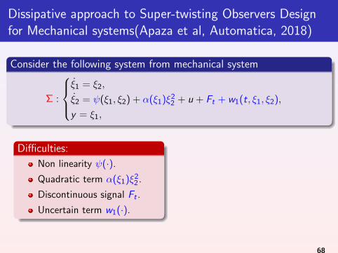
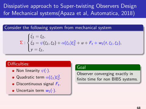
Dissipative approach to Super-twisting Observers Designfor Mechanical systems(Apaza et al, Automatica, 2018)
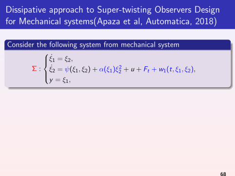
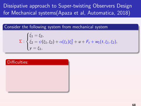
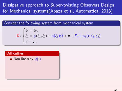
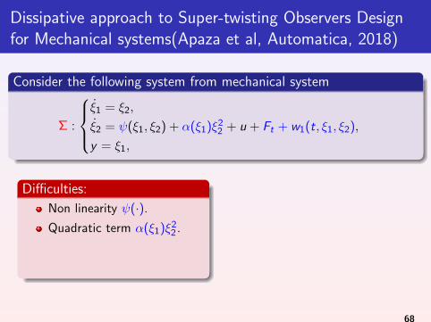
Consider the following system from mechanical system
Σ :
ξ1 = ξ2,
ξ2 = ψ(ξ1, ξ2) + α(ξ1)ξ22 + u + Ft + w1(t, ξ1, ξ2),
y = ξ1,
Difficulties:
Non linearity ψ(·).
Quadratic term α(ξ1)ξ22 .
Discontinuous signal Ft .
Uncertain term w1(·).
Goal
Observer converging exactly infinite time for non BIBS systems.
68

Dissipative approach to Super-twisting Observers Designfor Mechanical systems(Apaza et al, Automatica, 2018)
Consider the following system from mechanical system
Σ :
ξ1 = ξ2,
ξ2 = ψ(ξ1, ξ2) + α(ξ1)ξ22 + u + Ft + w1(t, ξ1, ξ2),
y = ξ1,
Difficulties:
Non linearity ψ(·).
Quadratic term α(ξ1)ξ22 .
Discontinuous signal Ft .
Uncertain term w1(·).
Goal
Observer converging exactly infinite time for non BIBS systems.
68
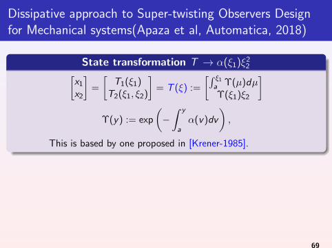
Dissipative approach to Super-twisting Observers Designfor Mechanical systems(Apaza et al, Automatica, 2018)
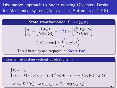
State transformation T → α(ξ1)ξ22[
x1
x2
]=
[T1(ξ1)
T2(ξ1, ξ2)
]= T (ξ) :=
[∫ ξ1
a Υ(µ)dµΥ(ξ1)ξ2
]Υ(y) := exp
(−∫ y
aα(v)dv
),
This is based by one proposed in [Krener-1985].
Transformed system without quadratic term
{x1 = x2,
x2 = Υ(yT
)ψ(yT, (Υ(y
T))−1x2) + Υ(y
T)u + Υ(y
T)w(t, ξ1, ξ2),
yT
:= T−11 (x1), w(t, ξ1, ξ2) := Ft + w1(t, ξ1, ξ2)
69
Dissipative approach to Super-twisting Observers Designfor Mechanical systems(Apaza et al, Automatica, 2018)
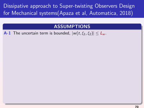
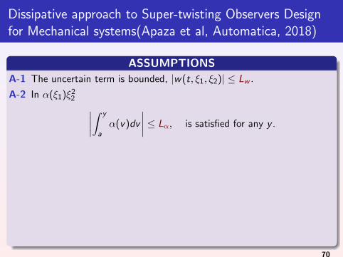
ASSUMPTIONS
A-1 The uncertain term is bounded, |w(t, ξ1, ξ2)| ≤ Lw .
A-2 In α(ξ1)ξ22 ∣∣∣∣∫ y
aα(v)dv
∣∣∣∣ ≤ Lα, is satisfied for any y .
A-3 There exists {q, s, r}, with q < 0, such that the nonlinearity
Γ(v1, v2, v3) := ψ(v1, v2 + v3)− ψ(v1, v2)
is {q, s, r}−dissipative, i.e.[Γ(v1, v2, v3)
v3
]T [q ss r
] [Γ(v1, v2, v3)
v3
]≥ 0, ∀ v1, v2, v3 ∈ R.
70
Dissipative approach to Super-twisting Observers Designfor Mechanical systems(Apaza et al, Automatica, 2018)
ASSUMPTIONS
A-1 The uncertain term is bounded, |w(t, ξ1, ξ2)| ≤ Lw .
A-2 In α(ξ1)ξ22 ∣∣∣∣∫ y
aα(v)dv
∣∣∣∣ ≤ Lα, is satisfied for any y .
A-3 There exists {q, s, r}, with q < 0, such that the nonlinearity
Γ(v1, v2, v3) := ψ(v1, v2 + v3)− ψ(v1, v2)
is {q, s, r}−dissipative, i.e.[Γ(v1, v2, v3)
v3
]T [q ss r
] [Γ(v1, v2, v3)
v3
]≥ 0, ∀ v1, v2, v3 ∈ R.
70
Dissipative approach to Super-twisting Observers Designfor Mechanical systems(Apaza et al, Automatica, 2018)
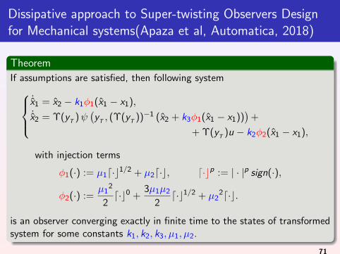
Theorem
If assumptions are satisfied, then following system˙x1 = x2 − k1φ1(x1 − x1),˙x2 = Υ(y
T)ψ(y
T, (Υ(y
T))−1 (x2 + k3φ1(x1 − x1))
)+
+ Υ(yT
)u − k2φ2(x1 − x1),
with injection terms
φ1(·) := µ1d·c1/2 + µ2d·c, d·cp := | · |p sign(·),
φ2(·) :=µ1
2
2d·c0 +
3µ1µ2
2d·c1/2 + µ2
2d·c.
is an observer converging exactly in finite time to the states of transformedsystem for some constants k1, k2, k3, µ1, µ2.
71
Dissipative approach to Super-twisting Observers Designfor Mechanical systems(Apaza et al, Automatica, 2018)
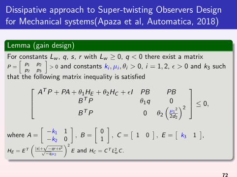
Lemma (gain design)
For constants Lw , q, s, r with Lw ≥ 0, q < 0 there exist a matrix
P =
[p1 p2
p2 p3
]> 0 and constants ki , µi , θi > 0, i = 1, 2, ε > 0 and k3 such
that the following matrix inequality is satisfied AT P + PA + θ1HE + θ2HC + εI PB PBBT P θ1q 0
BT P 0 θ2
(µ1
2
2d2
)2
≤ 0,
where A =
[−k1 1−k2 0
], B =
[01
], C =
[1 0
], E =
[k3 1
],
HE = E T
(|s|+√−qr+s2
√−qµ2
)2
E and HC = C T L2w C .
72
Outline
1 Conventional Sliding Mode Observers
2 Higher Order Sliding Mode Observers
3 Cascaded HOSM Observers for Linear systems with unknown inputs
4 Super-twisting based Observers for Mechanical Systems
5 HOSM based Observers for Nonlinear SystemsObservers for BIBS nonlinear systems with unknown inputs
6 Output-feedback finite-time stabilization of disturbed LTI systems
7 Unknown input identification
8 Parameter Identification
9 Output-based stabilization of disturbed systems
10 Switched Systems
11 Fault detection
73
Observer for nonlinear system with unknown inputs
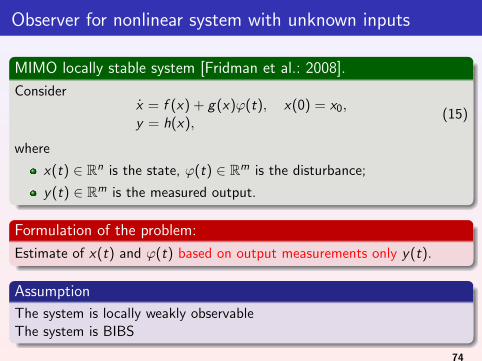
MIMO locally stable system [Fridman et al.: 2008].
Considerx = f (x) + g(x)ϕ(t), x(0) = x0,y = h(x),
(15)
where
x(t) ∈ Rn is the state, ϕ(t) ∈ Rm is the disturbance;
y(t) ∈ Rm is the measured output.
Formulation of the problem:
Estimate of x(t) and ϕ(t) based on output measurements only y(t).
Assumption
The system is locally weakly observableThe system is BIBS
74
Outline
5 HOSM based Observers for Nonlinear SystemsObservers for BIBS nonlinear systems with unknown inputs
75
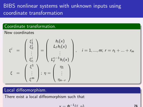
BIBS nonlinear systems with unknown inputs usingcoordinate transformation
Coordinate transformation.
New coordinates
ξi =
ξi
1
ξi2...ξi
ri
=
hi (x)
Lf hi (x)...
Lri−1f hi (x)
, i = 1, ...,m; r = r1 + ...+ rm
ξ =
ξ1
...ξm
; η =
η1...
ηn−r
Local diffeomorphism.
There exist a local diffeomorphism such that
x = Φ−1(ξ, η)
.
76
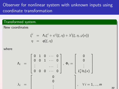
Observer for nonlinear system with unknown inputs usingcoordinate transformation
Transformed system.
New coordinates
ξi = Λiξi + ψi (ξ, η) + λi (ξ, η, ϕ(x))
η = q(ξ, η)
where
Λi =
0 1 0 · · · 00 0 1 · · · 0... · · ·
...0 0 0 · · · 0
, Φi =
00...
Lrif hi (x)
λi =
00...∑m
j=1 Lgi Lf ri−1hi (x)ϕ(x)j
, ∀ i = 1, ...,m77
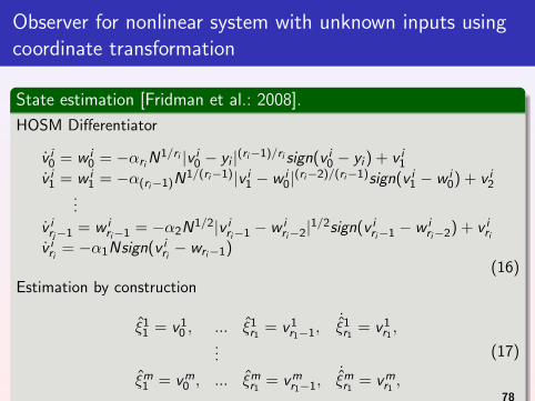
Observer for nonlinear system with unknown inputs usingcoordinate transformation
State estimation [Fridman et al.: 2008].
HOSM Differentiator
v i0 = w i
0 = −αri N1/ri |v i
0 − yi |(ri−1)/ri sign(v i0 − yi ) + v i
1
v i1 = w i
1 = −α(ri−1)N1/(ri−1)|v i1 − w i
0|(ri−2)/(ri−1)sign(v i1 − w i
0) + v i2
...
v iri−1 = w i
ri−1 = −α2N1/2|v iri−1 − w i
ri−2|1/2sign(v iri−1 − w i
ri−2) + v iri
v iri
= −α1Nsign(v iri− wri−1)
(16)Estimation by construction
ξ11 = v 1
0 , ... ξ1r1
= v 1r1−1,
˙ξ1
r1= v 1
r1,
...
ξm1 = v m
0 , ... ξmr1
= v mr1−1,
˙ξm
r1= v m
r1,
(17)
˙η = q(ξ, η)
78
Observers for BIBS systems with unknown inputs usingcoordinate transformation
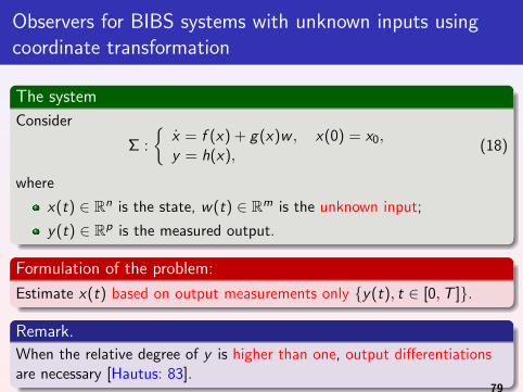
The system
Consider
Σ :
{x = f (x) + g(x)w , x(0) = x0,y = h(x),
(18)
where
x(t) ∈ Rn is the state, w(t) ∈ Rm is the unknown input;
y(t) ∈ Rp is the measured output.
Formulation of the problem:
Estimate x(t) based on output measurements only {y(t), t ∈ [0,T ]}.
Remark.
When the relative degree of y is higher than one, output differentiationsare necessary [Hautus: 83].
79
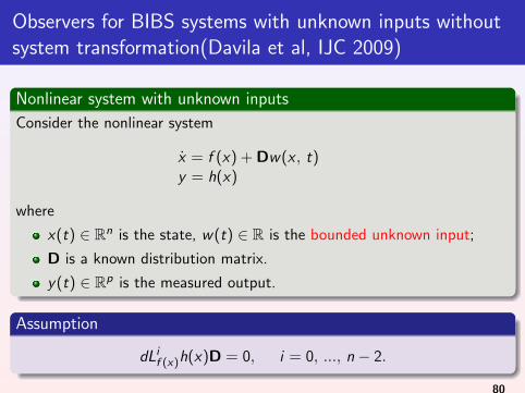
Observers for BIBS systems with unknown inputs withoutsystem transformation(Davila et al, IJC 2009)
Nonlinear system with unknown inputs
Consider the nonlinear system
x = f (x) + Dw(x , t)y = h(x)
where
x(t) ∈ Rn is the state, w(t) ∈ R is the bounded unknown input;
D is a known distribution matrix.
y(t) ∈ Rp is the measured output.
Assumption
dLif (x)h(x)D = 0, i = 0, ..., n − 2.
80
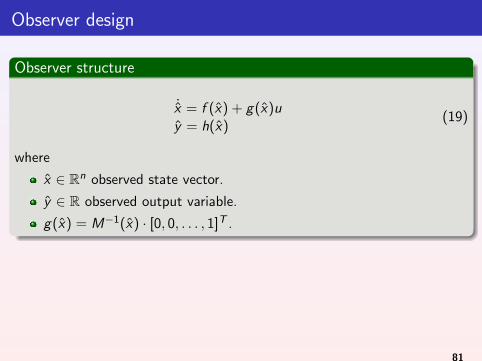
Observer design
Observer structure
˙x = f (x) + g(x)uy = h(x)
(19)
where
x ∈ Rn observed state vector.
y ∈ R observed output variable.
g(x) = M−1(x) · [0, 0, . . . , 1]T .
81
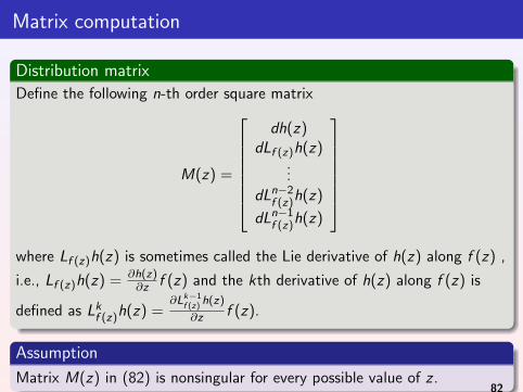
Matrix computation
Distribution matrix
Define the following n-th order square matrix
M(z) =
dh(z)
dLf (z)h(z)...
dLn−2f (z)h(z)
dLn−1f (z)h(z)
where Lf (z)h(z) is sometimes called the Lie derivative of h(z) along f (z) ,
i.e., Lf (z)h(z) = ∂h(z)∂z f (z) and the kth derivative of h(z) along f (z) is
defined as Lkf (z)h(z) =
∂Lk−1f (z)
h(z)
∂z f (z).
Assumption
Matrix M(z) in (82) is nonsingular for every possible value of z .82
Observers for systems with unknown inputs
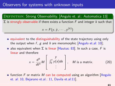
Definition: Strong Observability. [Angulo et. al.: Automatica 13]
Σ is strongly observable if there exists a function F and integer k such that
x = F (y , y , · · · , y (k))
equivalent to the distinguishability of the state trajectory using onlythe output when f , g and h are meromorphic [Angulo et.al: 10];
also equivalent when Σ is linear [Hautus: 83]. In such a case, F islinear and therefore
x =dk
dtkM
y∫ t0 y(s)ds
...
, M is a matrix. (20)
function F or matrix M can be computed using an algorithm [Anguloet. al: 10, Bejarano et.al.: 11, Davila et.al:11].
83
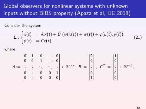
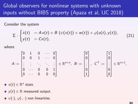
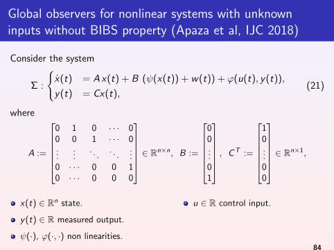
Global observers for nonlinear systems with unknowninputs without BIBS property (Apaza et al, IJC 2018)
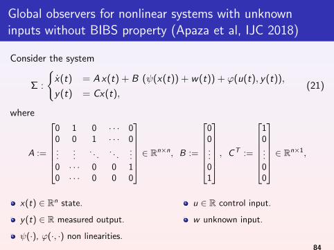
Consider the system
Σ :
{x(t) = A x(t) + B (ψ(x(t)) + w(t)) + ϕ(u(t), y(t)),
y(t) = Cx(t),(21)
where
A :=
0 1 0 · · · 00 0 1 · · · 0...
.... . .
. . ....
0 · · · 0 0 10 · · · 0 0 0
∈ Rn×n, B :=
00...01
, C T :=
10...00
∈ Rn×1,
x(t) ∈ Rn state.
y(t) ∈ R measured output.
ψ(·), ϕ(·, ·) non linearities.
u ∈ R control input.
w unknown input.
(21) is forward complete.
84

Global observers for nonlinear systems with unknowninputs without BIBS property (Apaza et al, IJC 2018)
Consider the system
Σ :
{x(t) = A x(t) + B (ψ(x(t)) + w(t)) + ϕ(u(t), y(t)),
y(t) = Cx(t),(21)
where
A :=
0 1 0 · · · 00 0 1 · · · 0...
.... . .
. . ....
0 · · · 0 0 10 · · · 0 0 0
∈ Rn×n, B :=
00...01
, C T :=
10...00
∈ Rn×1,
x(t) ∈ Rn state.
y(t) ∈ R measured output.
ψ(·), ϕ(·, ·) non linearities.
u ∈ R control input.
w unknown input.
(21) is forward complete.
84

Global observers for nonlinear systems with unknowninputs without BIBS property (Apaza et al, IJC 2018)
Consider the system
Σ :
{x(t) = A x(t) + B (ψ(x(t)) + w(t)) + ϕ(u(t), y(t)),
y(t) = Cx(t),(21)
where
A :=
0 1 0 · · · 00 0 1 · · · 0...
.... . .
. . ....
0 · · · 0 0 10 · · · 0 0 0
∈ Rn×n, B :=
00...01
, C T :=
10...00
∈ Rn×1,
x(t) ∈ Rn state.
y(t) ∈ R measured output.
ψ(·), ϕ(·, ·) non linearities.
u ∈ R control input.
w unknown input.
(21) is forward complete.84
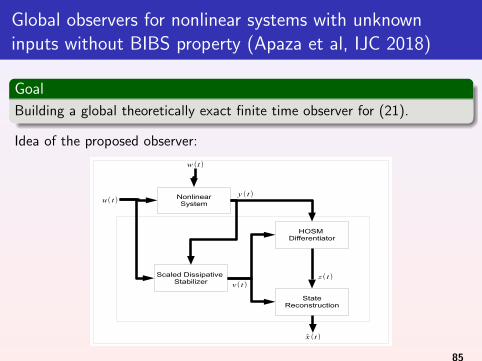
Global observers for nonlinear systems with unknowninputs without BIBS property (Apaza et al, IJC 2018)
Goal
Building a global theoretically exact finite time observer for (21).
Idea of the proposed observer:
NonlinearSystem
Scaled Dissipative Stabilizer
HOSM Differentiator
u (t)
w (t)
y (t)
v(t)
StateReconstruction
z(t)
x (t)
85
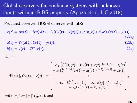
Global observers for nonlinear systems with unknowninputs without BIBS property (Apaza et al, IJC 2018)
Proposed observer: HOSM observer with SDS
v(t) = Av(t) + Bψ(v(t) + N(Cv(t)− y(t))) + ϕ(u, y) + ∆l K (Cv(t)− y(t)),(22a)
z(t) = W (z(t),Cv(t)− y(t)), (22b)
x(t) = v(t)−O−1z(t), (22c)
where
W (z(t),Cv(t)− y(t)) :=
−α1L
1/nf dz1(t)− Cv(t) + y(t)c(n−1)/n + z2(t)
−α2L1/(n−1)f dz2(t)− z1(t)c(n−2)/(n−1) + z3(t)
...
−αn−1L1/2f dzn−1(t)− zn−2(t)c1/2 + zn(t)−αnLf dzn(t)− zn−1(t)c0
,
with d◦cs := | ◦ |s sign(◦), and
86
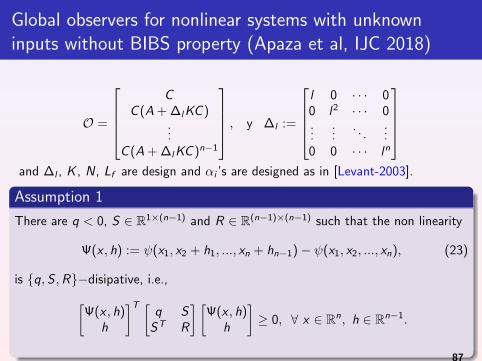
Global observers for nonlinear systems with unknowninputs without BIBS property (Apaza et al, IJC 2018)
O =
C
C (A + ∆l KC )...
C (A + ∆l KC )n−1
, y ∆l :=
l 0 · · · 00 l2 · · · 0...
.... . .
...0 0 · · · ln
and ∆l , K , N, Lf are design and αi ’s are designed as in [Levant-2003].
Assumption 1
There are q < 0, S ∈ R1×(n−1) and R ∈ R(n−1)×(n−1) such that the non linearity
Ψ(x , h) := ψ(x1, x2 + h1, ..., xn + hn−1)− ψ(x1, x2, ..., xn), (23)
is {q,S ,R}−disipative, i.e.,[Ψ(x , h)
h
]T [q S
ST R
] [Ψ(x , h)
h
]≥ 0, ∀ x ∈ Rn, h ∈ Rn−1.
87
Global observers for nonlinear systems with unknowninputs without BIBS property (Apaza et al, IJC 2018)
Theorem
If the assumption 1 is satisfied, then
i) there exist matrices P = PT > 0 and Q = QT > 0 with P,Q ∈ Rn×n,
K ∈ Rn, N =[N2 · · · N3
]T ∈ R(n−1) and scalars ε > 0, l0 ≥ 1 such thatthe inequalityl
(PAK + AT
K P + εQ +1
l2n(In∆l )
TlN
R(In∆l )lN
)?
BT P +1
l2n−1S(In∆l )lN lq
≤ 0,
is satisfied for all l ≥ l0, where
In :=
0 1 0 · · · 00 0 1 · · · 0...
.... . .
. . ....
0 · · · 0 0 1
∈ R(n−1)×n, AK := A + KC , y
(In∆l )lN := In∆l + l NC .
88

Global observers for nonlinear systems with unknowninputs without BIBS property (Apaza et al, IJC 2018)
Theorem
If the assumption 1 is satisfied, then
i) there exist matrices P = PT > 0 and Q = QT > 0 with P,Q ∈ Rn×n,
K ∈ Rn, N =[N2 · · · N3
]T ∈ R(n−1) and scalars ε > 0, l0 ≥ 1 such thatthe inequalityl
(PAK + AT
K P + εQ +1
l2n(In∆l )
TlN
R(In∆l )lN
)?
BT P +1
l2n−1S(In∆l )lN lq
≤ 0,
is satisfied for all l ≥ l0, where
In :=
0 1 0 · · · 00 0 1 · · · 0...
.... . .
. . ....
0 · · · 0 0 1
∈ R(n−1)×n, AK := A + KC , y
(In∆l )lN := In∆l + l NC . 88

Global observers for nonlinear systems with unknowninputs without BIBS property (Apaza et al, IJC 2018)
ii) the estimation error is finally uniform bounded with final bound
‖ev‖ <b
l, for all l ≥ l0, (24)
where b := 2‖PB‖%w
ελmın(Q)
√λmax(P)λmın(P) n.
iii) the n−th time derive evy = Cv − y is bounded, with bound
Lf =
{2‖PB‖+ δ
ελmın(Q)
[∥∥∥∥(A + KC )nG T diag
{λmax(P)
λi (P)
}∥∥∥∥√n+
+ %ψ
∥∥∥∥(In + NC )∆l
ln+1G T
∥∥∥∥]+ 1
}%w , (25)
%ψ = 1√−q
(√−λmax(R)q + λmax(ST S) + {λmax(ST S)}1/2
), G a
orthogonal matrix D = diag{λi (P)} where λi (P) denotes the eigenvalue of
matrix P for i = 1, ..., n such that P = G T DG .
89
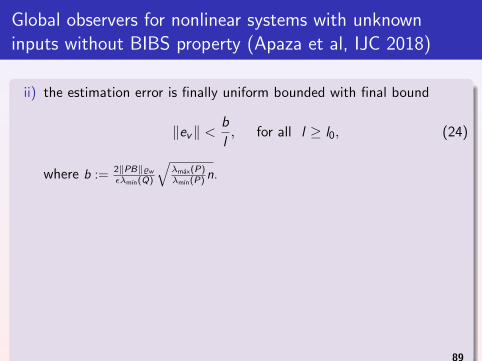
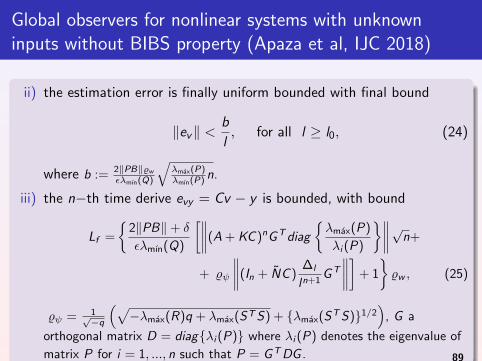
Global observers for nonlinear systems with unknowninputs without BIBS property (Apaza et al, IJC 2018)
ii) the estimation error is finally uniform bounded with final bound
‖ev‖ <b
l, for all l ≥ l0, (24)
where b := 2‖PB‖%w
ελmın(Q)
√λmax(P)λmın(P) n.
iii) the n−th time derive evy = Cv − y is bounded, with bound
Lf =
{2‖PB‖+ δ
ελmın(Q)
[∥∥∥∥(A + KC )nG T diag
{λmax(P)
λi (P)
}∥∥∥∥√n+
+ %ψ
∥∥∥∥(In + NC )∆l
ln+1G T
∥∥∥∥]+ 1
}%w , (25)
%ψ = 1√−q
(√−λmax(R)q + λmax(ST S) + {λmax(ST S)}1/2
), G a
orthogonal matrix D = diag{λi (P)} where λi (P) denotes the eigenvalue of
matrix P for i = 1, ..., n such that P = G T DG . 89
Global observers for nonlinear systems with unknowninputs without BIBS property (Apaza et al, IJC 2018)
iii) the estimated state x in (22c) converges globally theoretic exact andin finite time to the real state x of (21).
Algorithm: design of HOSM observer with SDS
a) Choose K such that AK is Hurwitz.
b) Choose Q = QT > 0, N and ε > 0.
c) Find P = PT > 0 such that the Lyapunov inequalityPAK + AT
K P + εQ + Λ%ψ < 0, with
Λ%ψ := diag
{%ψ
(n − i + 1)2
}para i = 1, ..., n, is satisfied.
d) Increase the value l until the matrix inequality is satisfied.
e) Find the orthogonal matrix G and diagonal matrix D correspondingto P such that P = G T DG .
f) Define Lf in (25) and the matrix O−1.
90
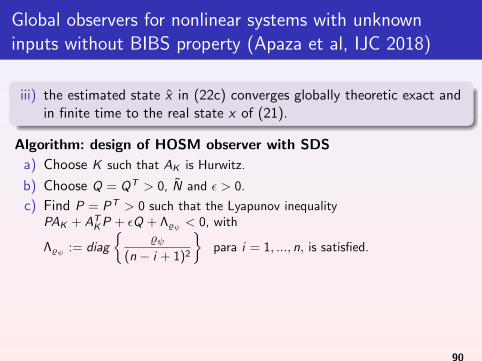
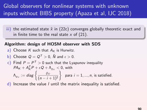
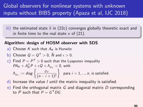
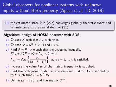
Outline
1 Conventional Sliding Mode Observers
2 Higher Order Sliding Mode Observers
3 Cascaded HOSM Observers for Linear systems with unknown inputs
4 Super-twisting based Observers for Mechanical Systems
5 HOSM based Observers for Nonlinear Systems
6 Output-feedback finite-time stabilization of disturbed LTI systems
7 Unknown input identification
8 Parameter Identification
9 Output-based stabilization of disturbed systems
10 Switched Systems
11 Fault detection
91
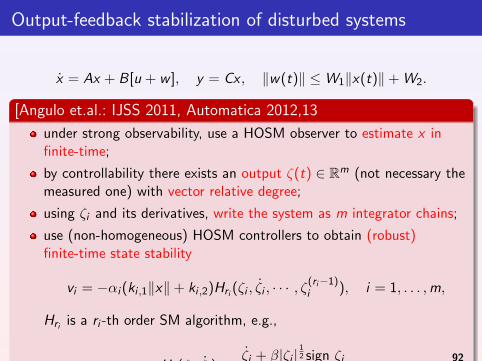
Output-feedback stabilization of disturbed systems
x = Ax + B[u + w ], y = Cx , ‖w(t)‖ ≤W1‖x(t)‖+ W2.
[Angulo et.al.: IJSS 2011, Automatica 2012,13
under strong observability, use a HOSM observer to estimate x infinite-time;
by controllability there exists an output ζ(t) ∈ Rm (not necessary themeasured one) with vector relative degree;
using ζi and its derivatives, write the system as m integrator chains;
use (non-homogeneous) HOSM controllers to obtain (robust)finite-time state stability
vi = −αi (ki ,1‖x‖+ ki ,2)Hri (ζi , ζi , · · · , ζ(ri−1)i ), i = 1, . . . ,m,
Hri is a ri -th order SM algorithm, e.g.,
H2(ζi , ζi ) :=ζi + β|ζi |
12 sign ζi
|ζi |+ β|ζi |12
.92
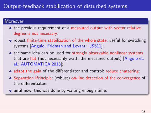
Output-feedback stabilization of disturbed systems
Moreover
the previous requirement of a measured output with vector relativedegree is not necessary;
robust finite-time stabilization of the whole state: useful for switchingsystems [Angulo, Fridman and Levant: IJSS11];
the same idea can be used for strongly observable nonlinear systemsthat are flat (not necessarily w.r.t. the measured output) [Angulo et.al.: AUTOMATICA,2013];
adapt the gain of the differentiator and control: reduce chattering;
Separation Principle: (robust) on-line detection of the convergence ofthe differentiators;
until now, this was done by waiting enough time.
93
Outline
1 Conventional Sliding Mode Observers
2 Higher Order Sliding Mode Observers
3 Cascaded HOSM Observers for Linear systems with unknown inputs
4 Super-twisting based Observers for Mechanical Systems
5 HOSM based Observers for Nonlinear Systems
6 Output-feedback finite-time stabilization of disturbed LTI systems
7 Unknown input identification
8 Parameter Identification
9 Output-based stabilization of disturbed systems
10 Switched Systems
11 Fault detection
94
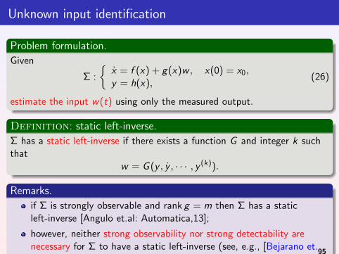
Unknown input identification
Problem formulation.
Given
Σ :
{x = f (x) + g(x)w , x(0) = x0,y = h(x),
(26)
estimate the input w(t) using only the measured output.
Definition: static left-inverse.
Σ has a static left-inverse if there exists a function G and integer k suchthat
w = G (y , y , · · · , y (k)).
Remarks.
if Σ is strongly observable and rank g = m then Σ has a staticleft-inverse [Angulo et.al: Automatica,13];
however, neither strong observability nor strong detectability arenecessary for Σ to have a static left-inverse (see, e.g., [Bejarano et.al.: SIAM 09] ).
95
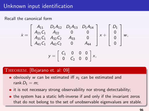
Unknown input identification
Recall the canonical form
x =
A11 D1A12 D1A13 D1A14
A21C1 A22 0 0A31C1 A32C2 A33 0A41C1 A42C2 0 A44
x +
D1
000
w ,
y =
[C1 0 0 00 C2 0 0
]x ,
Theorem. [Bejarano et. al: 09]
obviously w can be estimated iff x1 can be estimated andrank D1 = m;
it is not necessary strong observability nor strong detectability;
the system has a static left-inverse if and only if the invariant zerosthat do not belong to the set of unobservable eigenvalues are stable.
96
Outline
1 Conventional Sliding Mode Observers
2 Higher Order Sliding Mode Observers
3 Cascaded HOSM Observers for Linear systems with unknown inputs
4 Super-twisting based Observers for Mechanical Systems
5 HOSM based Observers for Nonlinear Systems
6 Output-feedback finite-time stabilization of disturbed LTI systems
7 Unknown input identification
8 Parameter Identification
9 Output-based stabilization of disturbed systems
10 Switched Systems
11 Fault detection
97
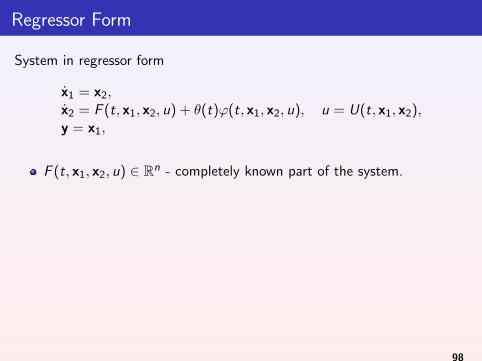
Regressor Form
System in regressor form
x1 = x2,x2 = F (t, x1, x2, u) + θ(t)ϕ(t, x1, x2, u), u = U(t, x1, x2),y = x1,
F (t, x1, x2, u) ∈ Rn - completely known part of the system.
θ(t) ∈ Rn×l - uncertain parameters.
ϕ(t, x1, x2, u) ∈ Rl - known nonlinear functions vector.
98
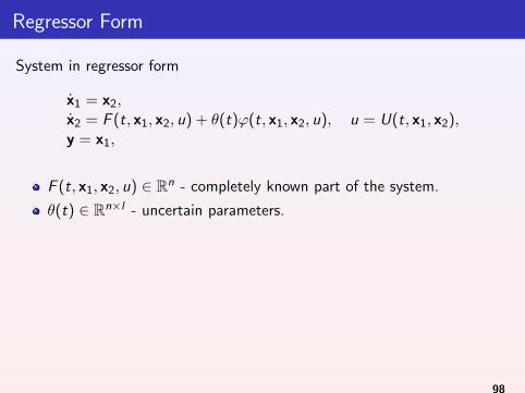
Regressor Form
System in regressor form
x1 = x2,x2 = F (t, x1, x2, u) + θ(t)ϕ(t, x1, x2, u), u = U(t, x1, x2),y = x1,
F (t, x1, x2, u) ∈ Rn - completely known part of the system.
θ(t) ∈ Rn×l - uncertain parameters.
ϕ(t, x1, x2, u) ∈ Rl - known nonlinear functions vector.
98
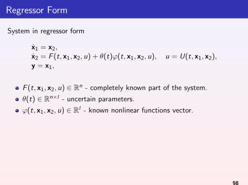
Regressor Form
System in regressor form
x1 = x2,x2 = F (t, x1, x2, u) + θ(t)ϕ(t, x1, x2, u), u = U(t, x1, x2),y = x1,
F (t, x1, x2, u) ∈ Rn - completely known part of the system.
θ(t) ∈ Rn×l - uncertain parameters.
ϕ(t, x1, x2, u) ∈ Rl - known nonlinear functions vector.
98

Observer
State observer
˙x1 = x2 + α2λ(x1)sign(x1)˙x2 = F (t, x1, x2, u) + θ(t)ϕ(t, x1, x2, u) + α1sign(x1),
θ ∈ Rn×l -nominal values of the parameters matrix θ(t).
99
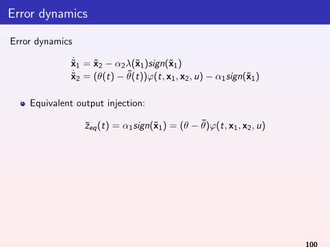
Error dynamics
Error dynamics
˙x1 = x2 − α2λ(x1)sign(x1)˙x2 = (θ(t)− θ(t))ϕ(t, x1, x2, u)− α1sign(x1)
Equivalent output injection:
zeq(t) = α1sign(x1) = (θ − θ)ϕ(t, x1, x2, u)
100
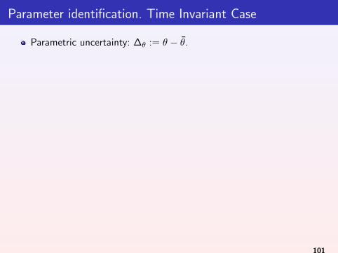
Parameter identification. Time Invariant Case
Parametric uncertainty: ∆θ := θ − θ.
Time invariant parameters identification (dynamic least-squaremethod):
˙∆θ =
[−∆θϕ(t) + zeq(t)
]ϕT (t)Γ(t).
WhereΓ(t) = −Γ(t)ϕ(t)ϕT (t)Γ(t)
101
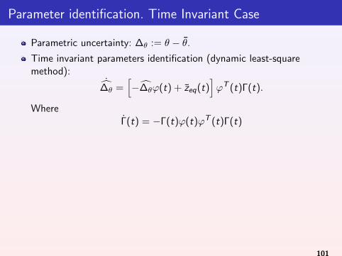
Parameter identification. Time Invariant Case
Parametric uncertainty: ∆θ := θ − θ.
Time invariant parameters identification (dynamic least-squaremethod):
˙∆θ =
[−∆θϕ(t) + zeq(t)
]ϕT (t)Γ(t).
WhereΓ(t) = −Γ(t)ϕ(t)ϕT (t)Γ(t)
101
Parameter identification. Time Variant Case
Parametric uncertainty: ϑ(t) = θ(t)− θ(t).
Time variant parameters identification (forgetting factor method):
˙ϑ(t) =(
zeq(t)− ϑ(t)ϕ(t))ϕT (t)Γ(t).
WhereΓ(t) = −
(Γ(t)ϕ(t)ϕT (t) + ln R
)Γ(t).
The matrix R = RT ∈ Rn×n is called the matrix forgetting factor,satisfying the conditions:
|λmin(R)| > 0,||R|| = % < 1.
102

Parameter identification. Time Variant Case
Parametric uncertainty: ϑ(t) = θ(t)− θ(t).
Time variant parameters identification (forgetting factor method):
˙ϑ(t) =(
zeq(t)− ϑ(t)ϕ(t))ϕT (t)Γ(t).
WhereΓ(t) = −
(Γ(t)ϕ(t)ϕT (t) + ln R
)Γ(t).
The matrix R = RT ∈ Rn×n is called the matrix forgetting factor,satisfying the conditions:
|λmin(R)| > 0,
||R|| = % < 1.
102
Parameter identification. Time Variant Case
Parametric uncertainty: ϑ(t) = θ(t)− θ(t).
Time variant parameters identification (forgetting factor method):
˙ϑ(t) =(
zeq(t)− ϑ(t)ϕ(t))ϕT (t)Γ(t).
WhereΓ(t) = −
(Γ(t)ϕ(t)ϕT (t) + ln R
)Γ(t).
The matrix R = RT ∈ Rn×n is called the matrix forgetting factor,satisfying the conditions:
|λmin(R)| > 0,||R|| = % < 1.
102

Outline
1 Conventional Sliding Mode Observers
2 Higher Order Sliding Mode Observers
3 Cascaded HOSM Observers for Linear systems with unknown inputs
4 Super-twisting based Observers for Mechanical Systems
5 HOSM based Observers for Nonlinear Systems
6 Output-feedback finite-time stabilization of disturbed LTI systems
7 Unknown input identification
8 Parameter Identification
9 Output-based stabilization of disturbed systemsEstimation of the disturbance.
10 Switched Systems
11 Fault detection
103
Outline
9 Output-based stabilization of disturbed systemsEstimation of the disturbance.
104
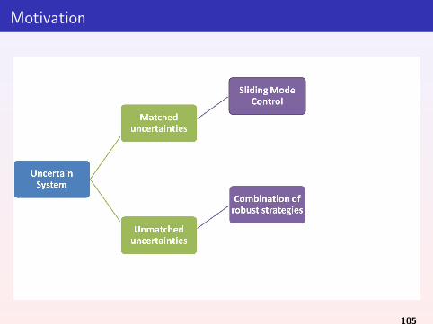
Motivation
105
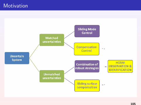
Motivation
105
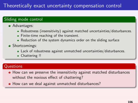
Theoretically exact uncertainty compensation control
Sliding mode control
Advantages:
Robustness (insensitivity) against matched uncertainties/disturbances.Finite-time reaching of the transient.Reduction of the system dynamics order on the sliding surface
Shortcomings:
Lack of robustness against unmatched uncertainties/disturbances.Chattering !!
Questions
How can we preserve the insensitivity against matched disturbanceswithout the noxious effect of chattering?
How can we deal against unmatched disturbances?
106
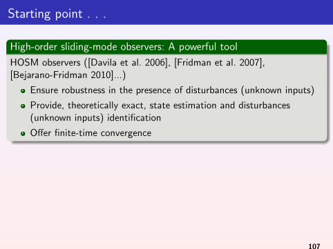
Starting point . . .
High-order sliding-mode observers: A powerful tool
HOSM observers ([Davila et al. 2006], [Fridman et al. 2007],[Bejarano-Fridman 2010]...)
Ensure robustness in the presence of disturbances (unknown inputs)
Provide, theoretically exact, state estimation and disturbances(unknown inputs) identification
Offer finite-time convergence
Output-feedback stabilization of disturbed systems
Using HOSMO to estimate in finite-time:
the state to design a robust controller
the state and identify the disturbance to compensate it through thecontrol signal
107
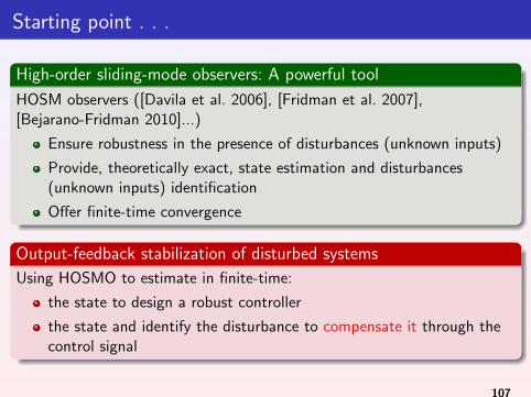
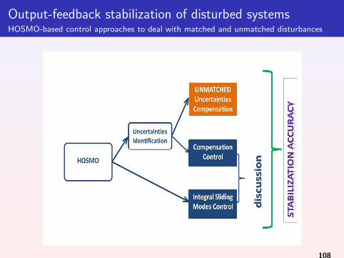
Output-feedback stabilization of disturbed systemsHOSMO-based control approaches to deal with matched and unmatched disturbances
108
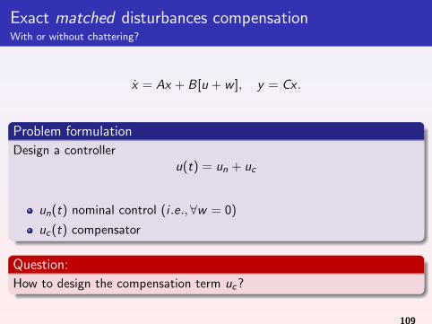
Exact matched disturbances compensationWith or without chattering?
x = Ax + B[u + w ], y = Cx .
Problem formulation
Design a controlleru(t) = un + uc
un(t) nominal control (i .e.,∀w = 0)
uc(t) compensator
Question:
How to design the compensation term uc ?
109
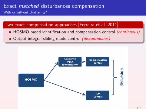
Exact matched disturbances compensationWith or without chattering?
Two exact compensation approaches [Ferreira et al. 2011]
HOSMO based identification and compensation control (continuous)
Output integral sliding mode control (discontinuous)
110
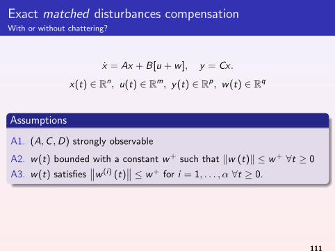
Exact matched disturbances compensationWith or without chattering?
x = Ax + B[u + w ], y = Cx .
x(t) ∈ Rn, u(t) ∈ Rm, y(t) ∈ Rp, w(t) ∈ Rq
Assumptions
A1. (A,C ,D) strongly observable
A2. w(t) bounded with a constant w + such that ‖w (t)‖ ≤ w + ∀t ≥ 0
A3. w(t) satisfies∥∥w (i) (t)
∥∥ ≤ w + for i = 1, . . . , α ∀t ≥ 0.
111
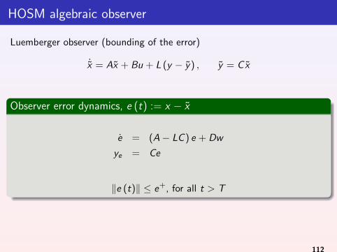
HOSM algebraic observer
Luemberger observer (bounding of the error)
˙x = Ax + Bu + L (y − y) , y = C x
Observer error dynamics, e (t) := x − x
e = (A− LC ) e + Dw
ye = Ce
‖e (t)‖ ≤ e+, for all t > T
112
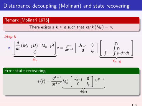
Disturbance decoupling (Molinari) and state recovering
Remark [Molinari 1976]
There exists a k ≤ n such that rank (Mk ) = n,
Step k
I
[d
dt(Mk−1D)⊥Mk−1A
C
]︸ ︷︷ ︸
Mk
e = dk−1
dtk−1
[Jk−1 0
0 Ip
] ye∫ye∫
. . .∫
yedτdt
︸ ︷︷ ︸
Y[k−1]
Error state recovering
e (t) =dk−1
dtk−1M+
k
[Jk−1 0
0 Ip
]Y
[k−1]
︸ ︷︷ ︸Θ(t)
113
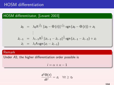
HOSM differentiation
HOSM differentitator, [Levant 2003]
z0 = λ0Λ1
i+1 ‖z0 −Θ (t)‖i
i+1 sgn (z0 −Θ (t)) + z1
...
zi−1 = λi−1Λ12 ‖zi−1 − zi−2‖
12 sgn (zi−1 − zi−2) + zi
zi = λi Λ sgn (zi − zi−1)
Remark
Under A3, the higher differentiation order possible is
i = α + κ− 1
d i Θ(t)
dt i= zi ∀t ≥ tf
114
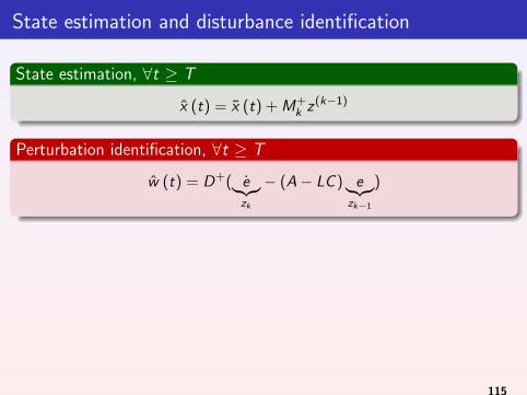
State estimation and disturbance identification
State estimation, ∀t ≥ T
x (t) = x (t) + M+k z(k−1)
Perturbation identification, ∀t ≥ T
w (t) = D+( e︸︷︷︸zk
− (A− LC ) e︸︷︷︸zk−1
)
115
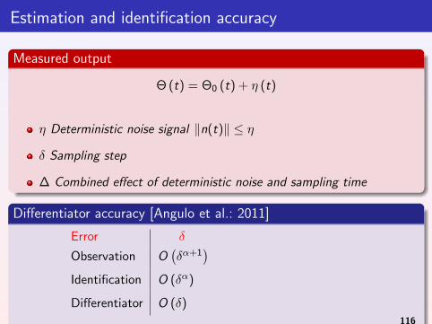
Estimation and identification accuracy
Measured output
Θ (t) = Θ0 (t) + η (t)
η Deterministic noise signal ‖n(t)‖ ≤ η
δ Sampling step
∆ Combined effect of deterministic noise and sampling time
Differentiator accuracy [Angulo et al.: 2011]
Error δ
η ∆
Observation O(δα+1
)
O(να+1α+k
)O(∆α+1
)
Identification O (δα)
O(ν
αα+k
)O (∆α)
Differentiator O (δ)
O(ν
1α+k
)O (∆)
116
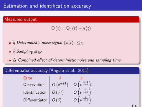
Estimation and identification accuracy
Measured output
Θ (t) = Θ0 (t) + η (t)
η Deterministic noise signal ‖n(t)‖ ≤ η
δ Sampling step
∆ Combined effect of deterministic noise and sampling time
Differentiator accuracy [Angulo et al.: 2011]
Error δ η
∆
Observation O(δα+1
)O(να+1α+k
)
O(∆α+1
)
Identification O (δα) O(ν
αα+k
)
O (∆α)
Differentiator O (δ) O(ν
1α+k
)
O (∆)
116
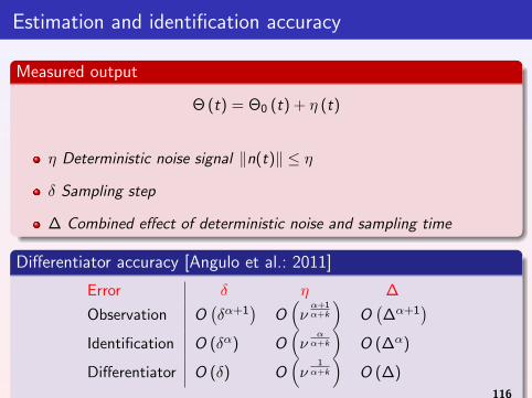
Estimation and identification accuracy
Measured output
Θ (t) = Θ0 (t) + η (t)
η Deterministic noise signal ‖n(t)‖ ≤ η
δ Sampling step
∆ Combined effect of deterministic noise and sampling time
Differentiator accuracy [Angulo et al.: 2011]
Error δ η ∆
Observation O(δα+1
)O(να+1α+k
)O(∆α+1
)Identification O (δα) O
(ν
αα+k
)O (∆α)
Differentiator O (δ) O(ν
1α+k
)O (∆)
116
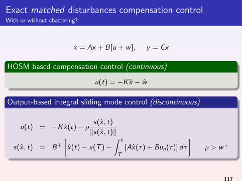
Exact matched disturbances compensation controlWith or without chattering?
x = Ax + B[u + w ], y = Cx
HOSM based compensation control (continuous)
u(t) = −K x − w
Output-based integral sliding mode control (discontinuous)
u(t) = −K x(t)− ρ s(x , t)
‖s(x , t)‖
s(x , t) = B+
[x(t)− x(T )−
∫ t
T[Ax(τ) + Bun(τ)] dτ
]ρ > w +
117
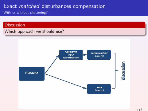
Exact matched disturbances compensationWith or without chattering?
Discussion
Which approach we should use?
118

Closed-loop system accuracy ε
HOSM identification and compensation control
ε = O(∆α+1
)︸ ︷︷ ︸Observation
+ O (∆α)︸ ︷︷ ︸Identification
+ O (µ)︸ ︷︷ ︸Execution
Output-based integral sliding mode control
ε = O(∆α+1
)︸ ︷︷ ︸Observation
+ O (µ)︸ ︷︷ ︸Execution
Where µ is the actuator time constant with an execution error O(µ)[Fridman: 02].
119
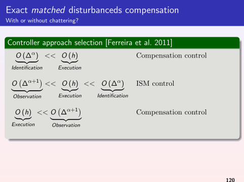
Exact matched disturbanceds compensationWith or without chattering?
Controller approach selection [Ferreira et al. 2011]
O (∆α)︸ ︷︷ ︸Identification
<< O (h)︸ ︷︷ ︸Execution
Compensation control
O(∆α+1
)︸ ︷︷ ︸Observation
<< O (h)︸ ︷︷ ︸Execution
<< O (∆α)︸ ︷︷ ︸Identification
ISM control
O (h)︸ ︷︷ ︸Execution
<< O(∆α+1
)︸ ︷︷ ︸Observation
Compensation control
120
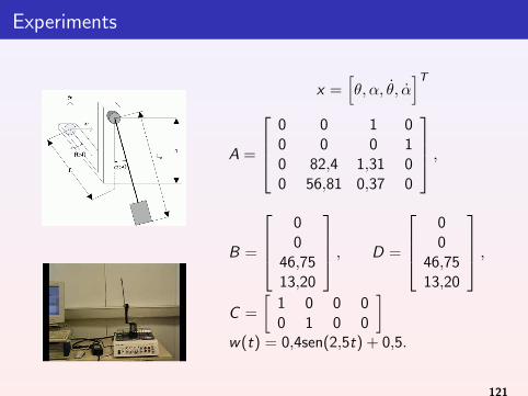
Experiments
x =[θ, α, θ, α
]T
A =
0 0 1 00 0 0 10 82,4 1,31 00 56,81 0,37 0
,
B =
00
46,7513,20
, D =
00
46,7513,20
,C =
[1 0 0 00 1 0 0
]w(t) = 0,4sen(2,5t) + 0,5.
121
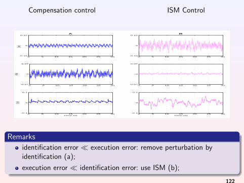
Compensation control ISM Control
0 5 10 15 20 25 30-0.15
0
0.15
( a )
A
0 5 10 15 20 25 30-0.15
0
0.15B
0 5 10 15 20 25 30-0.07
0
0.07
( b )
0 5 10 15 20 25 30-0.07
0
0.07
0 5 10 15 20 25 30-0.1
0
0.1
Time (s)
( c )
0 5 10 15 20 25 30-0.1
0
0.1
Time (s)
Remarks
identification error � execution error: remove perturbation byidentification (a);
execution error � identification error: use ISM (b);
122
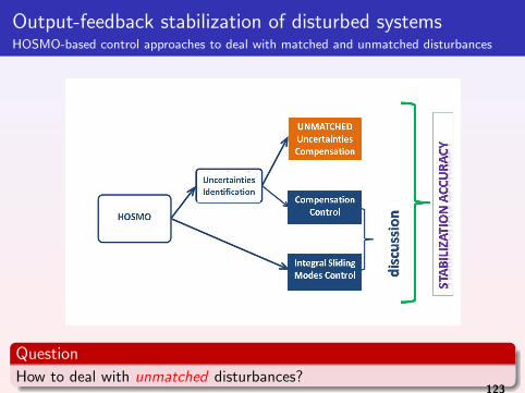
Output-feedback stabilization of disturbed systemsHOSMO-based control approaches to deal with matched and unmatched disturbances
Question
How to deal with unmatched disturbances?123
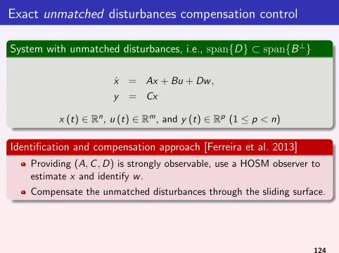
Exact unmatched disturbances compensation control
System with unmatched disturbances, i.e., span{D} ⊂ span{B⊥}
x = Ax + Bu + Dw ,
y = Cx
x (t) ∈ Rn, u (t) ∈ Rm, and y (t) ∈ Rp (1 ≤ p < n)
Identification and compensation approach [Ferreira et al. 2013]
Providing (A,C ,D) is strongly observable, use a HOSM observer toestimate x and identify w .
Compensate the unmatched disturbances through the sliding surface.
124
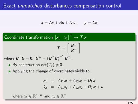
Exact unmatched disturbances compensation control
x = Ax + Bu + Dw , y = Cx
Coordinate transformation[x1 x2
]T 7→ Trx
Tr =
[B⊥
B+
]where B⊥B = 0, B+ =
(BT B
)−1BT .
By construction det(Tr ) 6= 0.
Applying the change of coordinates yields to
x1 = A11x1 + A12x2 + D1w
x2 = A21x1 + A22x2 + D2w + u
where x1 ∈ Rn−m and x2 ∈ Rm.
125
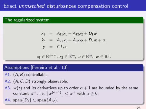
Exact unmatched disturbances compensation control
The regularized system
x1 = A11x1 + A12x2 + D1w
x2 = A21x1 + A22x2 + D2w + u
y = CTr x
x1 ∈ Rn−m, x2 ∈ Rm, u ∈ Rm, w ∈ Rq.
Assumptions [Ferreira et al.: 13]
A1. (A,B) controllable.
A2. (A,C ,D) strongly observable.
A3. w(t) and its derivatives up to order α + 1 are bounded by the sameconstant w +, i.e. ‖w (α+1)‖ < w + with α ≥ 0.
A4. span{D1} ⊂ span{A12}.
126
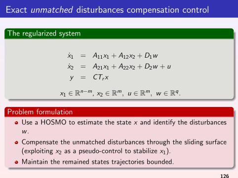
Exact unmatched disturbances compensation control
The regularized system
x1 = A11x1 + A12x2 + D1w
x2 = A21x1 + A22x2 + D2w + u
y = CTr x
x1 ∈ Rn−m, x2 ∈ Rm, u ∈ Rm, w ∈ Rq.
Problem formulation
Use a HOSMO to estimate the state x and identify the disturbancesw .
Compensate the unmatched disturbances through the sliding surface(exploiting x2 as a pseudo-control to stabilize x1).
Maintain the remained states trajectories bounded.
126
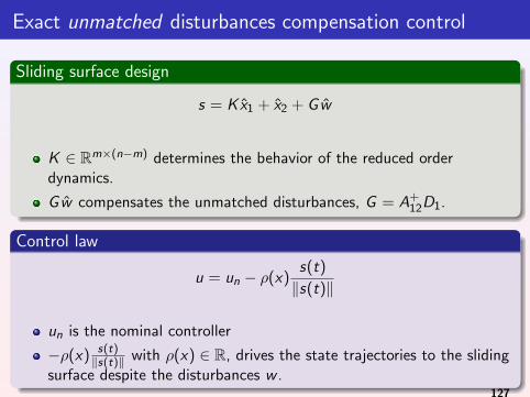
Exact unmatched disturbances compensation control
Sliding surface design
s = K x1 + x2 + G w
K ∈ Rm×(n−m) determines the behavior of the reduced orderdynamics.
G w compensates the unmatched disturbances, G = A+12D1.
Control law
u = un − ρ(x)s(t)
‖s(t)‖
un is the nominal controller
−ρ(x) s(t)‖s(t)‖ with ρ(x) ∈ R, drives the state trajectories to the sliding
surface despite the disturbances w .127
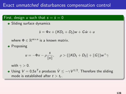
Exact unmatched disturbances compensation control
First, design u such that s = s = 0
Sliding surface dynamics
s = Φx + (KD1 + D2)w + G w + u
where Φ ∈ Rm×n is a known matrix.
Proposing
u = −Φx − ρ s
‖s‖, ρ > (‖KD1 + D2‖+ ‖G‖)w +γ
with γ > 0.
Using V = 0,5sT s produces V ≤ −γV 1/2. Therefore the slidingmode is established after t > tr .
128
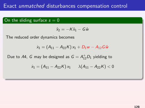
Exact unmatched disturbances compensation control
On the sliding surface s = 0
x2 = −K x1 − G w
The reduced order dynamics becomes
x1 = (A11 − A22K ) x1 + D1w − A12G w
Due to A4, G may be designed as G = A+12D1 yielding to
x1 = (A11 − A22K ) x1 λ(A11 − A22K ) < 0
129
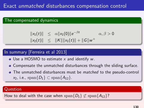
Exact unmatched disturbances compensation control
The compensated dynamics
‖x1(t)‖ ≤ α‖x1(0)‖e−βt α, β > 0
‖x2(t)‖ ≤ ‖K‖‖x1(t)‖+ ‖G‖w +
In summary [Ferreira et al 2013]
Use a HOSMO to estimate x and identify w .
Compensate the unmatched disturbances through the sliding surface.
The unmatched disturbances must be matched to the pseudo-controlx2, i.e., span{D1} ⊂ span{A12}.
Question
How to deal with the case when span{D1} 6⊂ span{A12}?
130
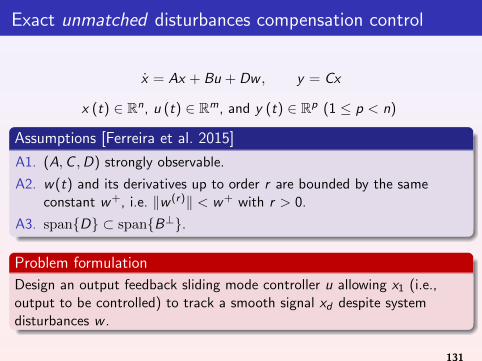
Exact unmatched disturbances compensation control
x = Ax + Bu + Dw , y = Cx
x (t) ∈ Rn, u (t) ∈ Rm, and y (t) ∈ Rp (1 ≤ p < n)
Assumptions [Ferreira et al. 2015]
A1. (A,C ,D) strongly observable.
A2. w(t) and its derivatives up to order r are bounded by the sameconstant w +, i.e. ‖w (r)‖ < w + with r > 0.
A3. span{D} ⊂ span{B⊥}.
Problem formulation
Design an output feedback sliding mode controller u allowing x1 (i.e.,output to be controlled) to track a smooth signal xd despite systemdisturbances w .
131
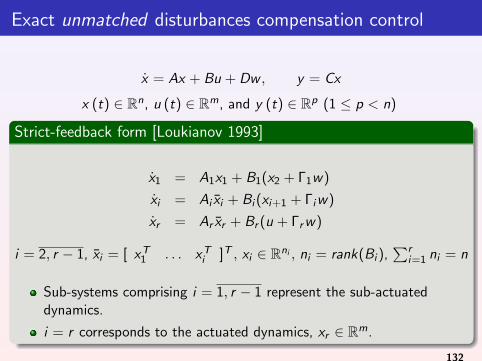
Exact unmatched disturbances compensation control
x = Ax + Bu + Dw , y = Cx
x (t) ∈ Rn, u (t) ∈ Rm, and y (t) ∈ Rp (1 ≤ p < n)
Strict-feedback form [Loukianov 1993]
x1 = A1x1 + B1(x2 + Γ1w)
xi = Ai xi + Bi (xi+1 + Γi w)
xr = Ar xr + Br (u + Γr w)
i = 2, r − 1, xi = [ xT1 . . . xT
i ]T , xi ∈ Rni , ni = rank(Bi ),∑r
i=1 ni = n
Sub-systems comprising i = 1, r − 1 represent the sub-actuateddynamics.
i = r corresponds to the actuated dynamics, xr ∈ Rm.
132
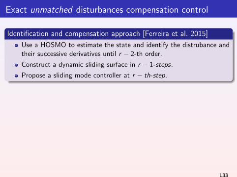
Exact unmatched disturbances compensation control
Identification and compensation approach [Ferreira et al. 2015]
Use a HOSMO to estimate the state and identify the distrubance andtheir successive derivatives until r − 2-th order.
Construct a dynamic sliding surface in r − 1-steps.
Propose a sliding mode controller at r − th-step.
133
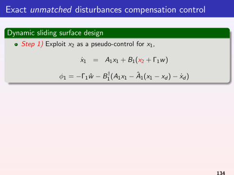
Exact unmatched disturbances compensation control
Dynamic sliding surface design
Step 1) Exploit x2 as a pseudo-control for x1,
x1 = A1x1 + B1(x2 + Γ1w)
φ1 = −Γ1w − B†1(A1x1 − A1(x1 − xd )− xd )
134
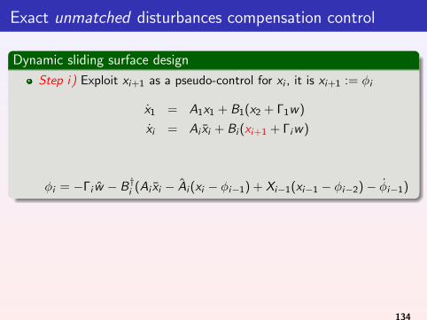
Exact unmatched disturbances compensation control
Dynamic sliding surface design
Step i) Exploit xi+1 as a pseudo-control for xi , it is xi+1 := φi
x1 = A1x1 + B1(x2 + Γ1w)
xi = Ai xi + Bi (xi+1 + Γi w)
φi = −Γi w − B†i (Ai xi − Ai (xi − φi−1) + Xi−1(xi−1 − φi−2)− φi−1)
134
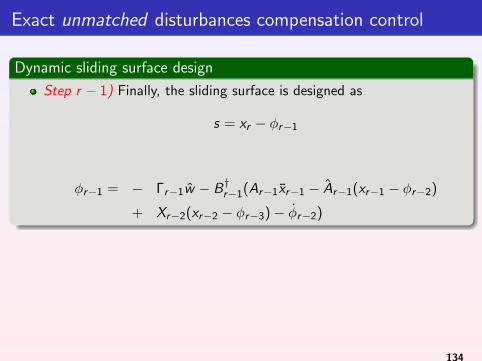
Exact unmatched disturbances compensation control
Dynamic sliding surface design
Step r − 1) Finally, the sliding surface is designed as
s = xr − φr−1
φr−1 = − Γr−1w − B†r−1(Ar−1xr−1 − Ar−1(xr−1 − φr−2)
+ Xr−2(xr−2 − φr−3)− φr−2)
134
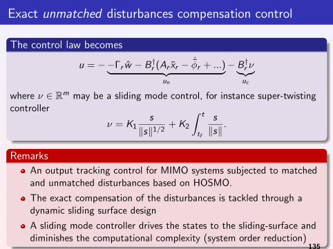
Exact unmatched disturbances compensation control
The control law becomes
u = −−Γr w − B†r (Ar xr − ˙φr + ...)︸ ︷︷ ︸un
− B†r ν︸︷︷︸uc
where ν ∈ Rm may be a sliding mode control, for instance super-twistingcontroller
ν = K1s
‖s‖1/2+ K2
∫ t
tf
s
‖s‖.
Remarks
An output tracking control for MIMO systems subjected to matchedand unmatched disturbances based on HOSMO.
The exact compensation of the disturbances is tackled through adynamic sliding surface design
A sliding mode controller drives the states to the sliding-surface anddiminishes the computational complexity (system order reduction)
135
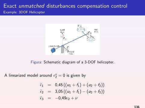
Exact unmatched disturbances compensation controlExample: 3DOF Helicopter
Figura: Schematic diagram of a 3-DOF helicopter.
A linearized model around ε∗2 = 0 is given by
ε1 = 0,45 ((u1 + f1) + (u2 + f2))
ε2 = 3,05 ((u1 + f1)− (u2 + f2))
ε3 = −0,49ε2 + ν
136
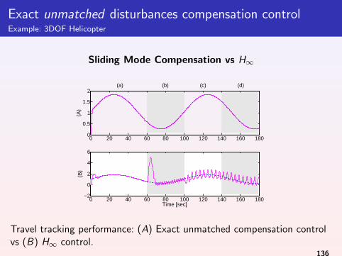
Exact unmatched disturbances compensation controlExample: 3DOF Helicopter
Sliding Mode Compensation vs H∞
0 20 40 60 80 100 120 140 160 1800
0.5
1
1.5
2
(A)
0 20 40 60 80 100 120 140 160 180−2
0
2
4
6
Time [sec]
(B)
(a) (b) (c) (d)
Travel tracking performance: (A) Exact unmatched compensation controlvs (B) H∞ control.
136
Outline
1 Conventional Sliding Mode Observers
2 Higher Order Sliding Mode Observers
3 Cascaded HOSM Observers for Linear systems with unknown inputs
4 Super-twisting based Observers for Mechanical Systems
5 HOSM based Observers for Nonlinear Systems
6 Output-feedback finite-time stabilization of disturbed LTI systems
7 Unknown input identification
8 Parameter Identification
9 Output-based stabilization of disturbed systems
10 Switched SystemsObservation of the continuous and discrete state of switched systemsLinear Switched Systems
11 Fault detection
137

Outline
10 Switched SystemsObservation of the continuous and discrete state of switched systemsLinear Switched Systems
138

Problem Statement
Consider the switched system:
x(t) = fσ(t)(x(t)) + Bσ(t)u(t) + Dσ(t)w(t), (27)
y(t) = hσ(t)(x(t)) (28)
x ∈ X ⊆ Rn, y ∈ Y ⊆ Rm, u ∈ U ⊆ Up, w ∈ W ⊆ Rm,σ ∈ Q ∈ ℵ,fσ(t) : Xσ → Rn, Bσ(t) ∈ Rn×p, Dσ(t) ∈ Rn×m, hσ(t) : Xσ → Y,
Autonomous. The dynamics changes discontinuously when x(t) hitscertain boundaries, i.e. σ depends on x(t).
Non-Autonomous. The dynamics changes abruptly in response to acontrol command or an exogenous signal, i.e. σ does not depends onx(t).
Main Objective
To develop some observation approaches for estimating thecontinuous and discrete states in certain classes of SS.
139
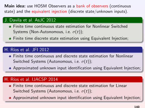
Main idea: use HOSM Observers as a bank of observers (continuousstate) and the equivalent injection (discrete state/unknown inputs).
J. Davila et al. AsJC 2012
Finite time continuous state estimation for Nonlinear SwitchedSystems (Non-Autonomous, i.e. σ(t));
Finite time discrete state estimation using Equivalent Injection;
H. Rıos et al. JFI 2012
Finite time continuous and discrete state estimation for NonlinearSwitched Systems (Autonomous, i.e. σ(t));
Approximated unknown input identification using Equivalent Injection;
H. Rıos et al. IJACSP 2014
Finite time continuous and discrete state estimation for LinearSwitched Systems (Autonomous, i.e. σ(t));
Approximated unknown input identification using Equivalent Injection;
140

Outline
10 Switched SystemsObservation of the continuous and discrete state of switched systemsLinear Switched Systems
141
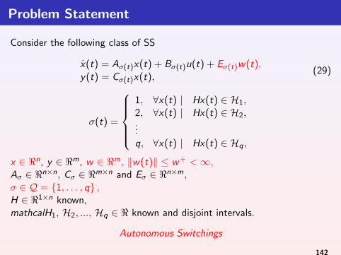
Problem Statement
Consider the following class of SS
x(t) = Aσ(t)x(t) + Bσ(t)u(t) + Eσ(t)w(t),y(t) = Cσ(t)x(t),
(29)
σ(t) =
1, ∀x(t) | Hx(t) ∈ H1,2, ∀x(t) | Hx(t) ∈ H2,...q, ∀x(t) | Hx(t) ∈ Hq,
x ∈ <n, y ∈ <m, w ∈ <m, ‖w(t)‖ ≤ w + <∞,Aσ ∈ <n×n, Cσ ∈ <m×n and Eσ ∈ <n×m,σ ∈ Q = {1, . . . , q} ,H ∈ <1×n known,mathcalH1, H2, ..., Hq ∈ < known and disjoint intervals.
Autonomous Switchings
142
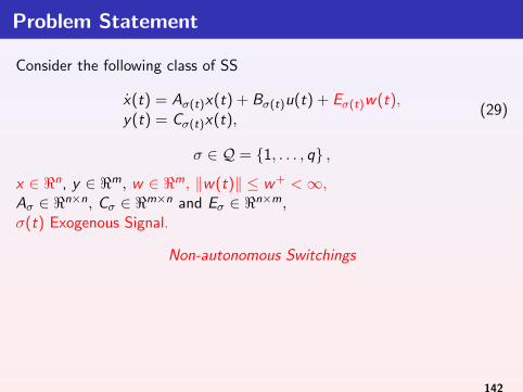
Problem Statement
Consider the following class of SS
x(t) = Aσ(t)x(t) + Bσ(t)u(t) + Eσ(t)w(t),y(t) = Cσ(t)x(t),
(29)
σ ∈ Q = {1, . . . , q} ,
x ∈ <n, y ∈ <m, w ∈ <m, ‖w(t)‖ ≤ w + <∞,Aσ ∈ <n×n, Cσ ∈ <m×n and Eσ ∈ <n×m,σ(t) Exogenous Signal.
Non-autonomous Switchings
142
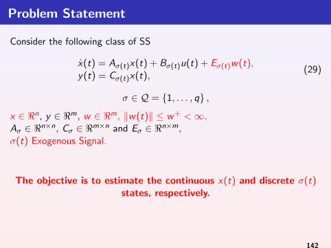
Problem Statement
Consider the following class of SS
x(t) = Aσ(t)x(t) + Bσ(t)u(t) + Eσ(t)w(t),y(t) = Cσ(t)x(t),
(29)
σ ∈ Q = {1, . . . , q} ,
x ∈ <n, y ∈ <m, w ∈ <m, ‖w(t)‖ ≤ w + <∞,Aσ ∈ <n×n, Cσ ∈ <m×n and Eσ ∈ <n×m,σ(t) Exogenous Signal.
The objective is to estimate the continuous x(t) and discrete σ(t)states, respectively.
142
Assumptions: Continuous State
1. The pair (Aσ,Cσ), ∀σ ∈ Q, is detectable.
2. The output has a r.d.v. (r1, . . . , rm) w.r.t. w , such thatr1 + · · ·+ rm = nV , ∀σ ∈ Q.
143
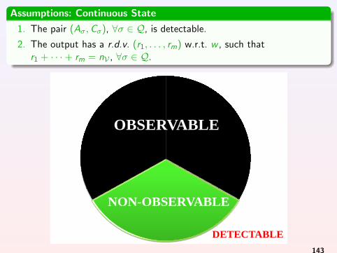
Assumptions: Continuous State
1. The pair (Aσ,Cσ), ∀σ ∈ Q, is detectable.
2. The output has a r.d.v. (r1, . . . , rm) w.r.t. w , such thatr1 + · · ·+ rm = nV , ∀σ ∈ Q.
No Fuertemente Observable
Fuertemente observable
OBSERVABLE
NON-OBSERVABLE
DETECTABLE
143
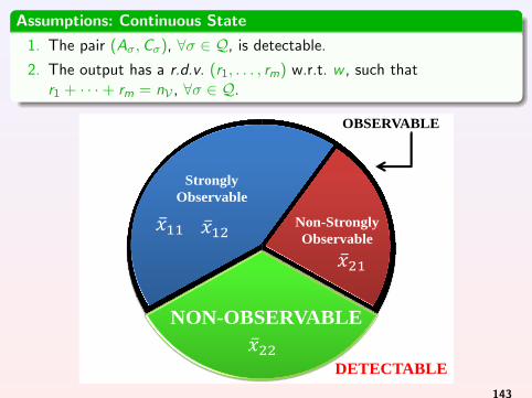
Assumptions: Continuous State
1. The pair (Aσ,Cσ), ∀σ ∈ Q, is detectable.
2. The output has a r.d.v. (r1, . . . , rm) w.r.t. w , such thatr1 + · · ·+ rm = nV , ∀σ ∈ Q.
Non-Strongly
Observable
Strongly
Observable
OBSERVABLE
𝑥 11 𝑥 12
𝑥 21
𝑥 22 DETECTABLE
NON-OBSERVABLE
143
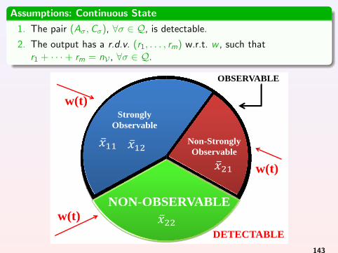
Assumptions: Continuous State
1. The pair (Aσ,Cσ), ∀σ ∈ Q, is detectable.
2. The output has a r.d.v. (r1, . . . , rm) w.r.t. w , such thatr1 + · · ·+ rm = nV , ∀σ ∈ Q.
OBSERVABLE
𝑥 11 𝑥 12
𝑥 21
𝑥 22 DETECTABLE
w(t)
w(t)
w(t)
NON-OBSERVABLE
Non-Strongly
Observable
Strongly
Observable
143
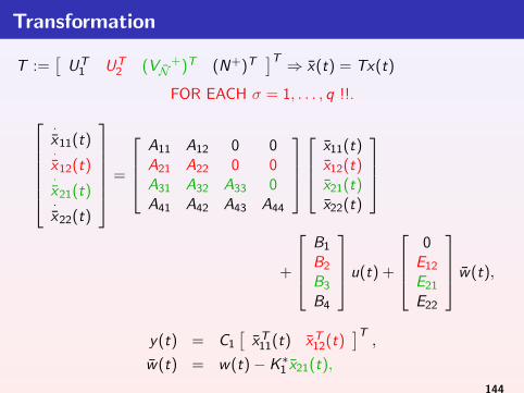
Transformation
T :=[
UT1 UT
2 (VN+)T (N+)T
]T ⇒ x(t) = Tx(t)
FOR EACH σ = 1, . . . , q !!.·x11(t)·x12(t)·x21(t)·x22(t)
=
A11 A12 0 0A21 A22 0 0A31 A32 A33 0A41 A42 A43 A44
x11(t)x12(t)x21(t)x22(t)
+
B1
B2
B3
B4
u(t) +
0
E12
E21
E22
w(t),
y(t) = C1
[xT
11(t) xT12(t)
]T,
w(t) = w(t)− K ∗1 x21(t),
144
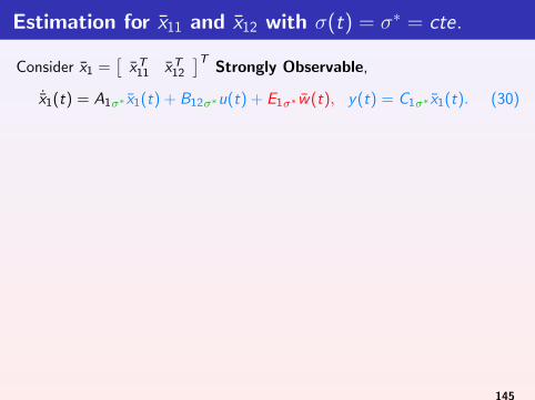
Estimation for x11 and x12 with σ(t) = σ∗ = cte.
Consider x1 =[
xT11 xT
12
]TStrongly Observable,
˙x1(t) = A1σ∗ x1(t) + B12σ∗u(t) + E1σ∗w(t), y(t) = C1σ∗ x1(t). (30)
Observer [L. Fridman et. al IJSS2007]
x1σ∗ (t) = z1σ∗ (t) + P1−1σ∗ νσ∗(t),
z1σ∗ (t) = A1σ∗z1σ∗(t) + B12σ∗u(t) + L1σ∗ (y(t)− C1σ∗z1σ∗(t)) ,
νσ∗(t) = Wσ∗(y(t)− C1σ∗z1σ∗(t), νσ∗(t)),
AL1σ∗ ⇒ (A1σ∗ − L1σ∗C1σ∗) Hurwitz.
P1σ∗ =[
c1Tσ∗ , (c1σ∗AL1σ∗)
T , · · · , (c1σ∗AL1
r1σ∗−1
σ∗ )T , · · · ,
cmTσ∗ , (cmσ∗AL1σ∗)
T , · · · , (cmσ∗AL1
rmσ∗−1
σ∗ )T]
T
⇒ rank(P1σ∗) = nVσ∗ .
145
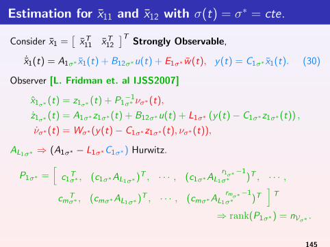
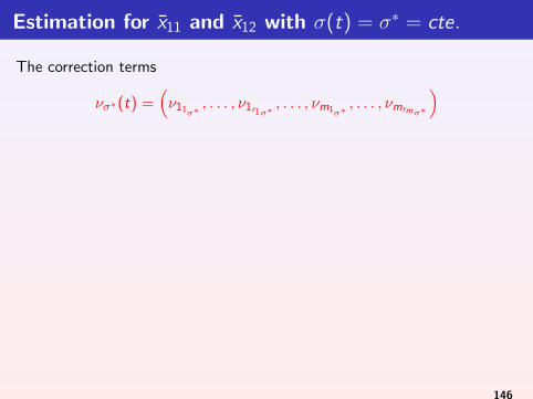
Estimation for x11 and x12 with σ(t) = σ∗ = cte.
The correction terms
νσ∗(t) =(ν11σ∗
, . . . , ν1r1σ∗, . . . , νm1σ∗
, . . . , νmrmσ∗
)
HOSM Differentiator [Levant and Livne TAC2012]
νk1σ∗= νk2σ∗
− αk1σ∗Mkσ∗ (t)
1rkσ∗
⌈νk1σ∗
− eykσ∗
⌋ rkσ∗−1
rkσ∗ ,
νkiσ∗= νk(i+1)σ∗
− αkiσ∗Mkσ∗ (t)
1rkσ∗−i+1
⌈νkiσ∗
− νk(i−1)σ∗
⌋ rkσ∗−i
rkσ∗−i+1,
∀i = 2, . . . , rkσ∗ − 1,
νkrkσ∗= −αkrkσ∗
Mkσ∗ (t)⌈νkrkσ∗
− νkrkσ∗−1
⌋0, ∀k = 1, . . . ,m,
where eykσ∗(t) = yk(t)− ckz1σ∗(t), the constants αkiσ∗
and the function
Mkσ∗ (t) are chosen recursively and sufficiently large.
146
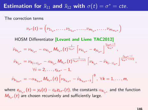
Estimation for x11 and x12 with σ(t) = σ∗ = cte.
The correction terms
νσ∗(t) =(ν11σ∗
, . . . , ν1r1σ∗, . . . , νm1σ∗
, . . . , νmrmσ∗
)HOSM Differentiator [Levant and Livne TAC2012]
νk1σ∗= νk2σ∗
− αk1σ∗Mkσ∗ (t)
1rkσ∗
⌈νk1σ∗
− eykσ∗
⌋ rkσ∗−1
rkσ∗ ,
νkiσ∗= νk(i+1)σ∗
− αkiσ∗Mkσ∗ (t)
1rkσ∗−i+1
⌈νkiσ∗
− νk(i−1)σ∗
⌋ rkσ∗−i
rkσ∗−i+1,
∀i = 2, . . . , rkσ∗ − 1,
νkrkσ∗= −αkrkσ∗
Mkσ∗ (t)⌈νkrkσ∗
− νkrkσ∗−1
⌋0, ∀k = 1, . . . ,m,
where eykσ∗(t) = yk (t)− ck z1σ∗(t), the constants αkiσ∗
and the function
Mkσ∗ (t) are chosen recursively and sufficiently large.
146
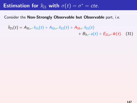
Estimation for x21 with σ(t) = σ∗ = cte.
Consider the Non-Strongly Observable but Observable part, i.e.
˙x21(t) = A31σ∗ x11(t) + A32σ∗ x12(t) + A33σ∗ x21(t)
+ B3σ∗u(t) + E21σ∗w(t). (31)
Let x21σ∗ (t) be the estimated state
x21σ∗ (t) = z2σ∗(t) + L2σ∗ x12σ∗ (t),z2σ∗ (t) = A1σ∗ x11σ∗ (t) + A2σ∗ x12σ∗ (t) + AL2σ∗ x21σ∗ (t) + B2σ∗u(t),
A1σ∗ = A31σ∗ − L2σ∗A21σ∗ ,
A2σ∗ = A32σ∗ − L2σ∗A22σ∗ ,
AL2σ∗ = A33σ∗ − K ∗1 σ∗E21σ∗ + L2σ∗E12σ∗K∗1 σ∗ ,
B2σ∗ = B3σ∗ − L2σ∗B2σ∗ .
147
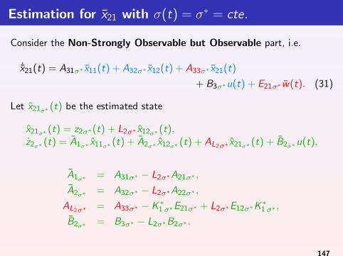
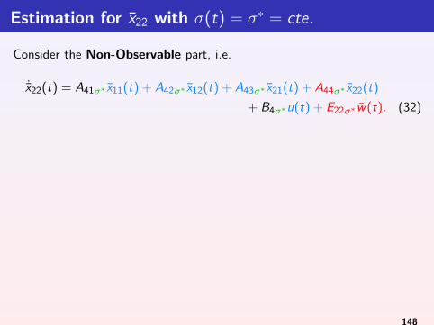
Estimation for x22 with σ(t) = σ∗ = cte.
Consider the Non-Observable part, i.e.
˙x22(t) = A41σ∗ x11(t) + A42σ∗ x12(t) + A43σ∗ x21(t) + A44σ∗ x22(t)
+ B4σ∗u(t) + E22σ∗w(t). (32)
Let x22σ∗ (t) be the estimated state
x22σ∗ (t) = z3σ∗(t) + E22σ∗E2+σ∗
[x12(t)x21(t)
],
z3σ∗ (t) = A41σ∗ x11σ∗ (t) + A42σ∗ x12σ∗ (t)+
A43σ∗ x21σ∗ (t) + A44σ∗ x22σ∗ (t) + B4σ∗u(t)
−E22σ∗E2+σ∗
[A21σ∗ x11σ∗ (t) + A22σ∗ x12σ∗ (t) + B2σ∗u(t)
A31σ∗ x11σ∗ (t) + A32σ∗ x12σ∗ (t) + A33σ∗ x21σ∗ (t) + B3σ∗u(t)
],
148
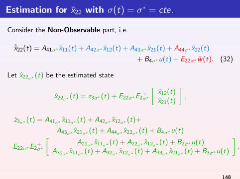
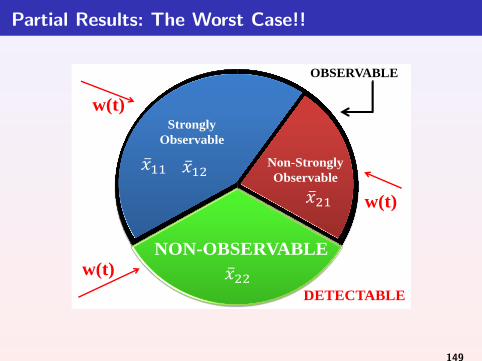
Partial Results: The Worst Case!!
OBSERVABLE
𝑥 11 𝑥 12
𝑥 21
𝑥 22 DETECTABLE
w(t)
w(t)
w(t)
NON-OBSERVABLE
Non-Strongly
Observable
Strongly
Observable
149
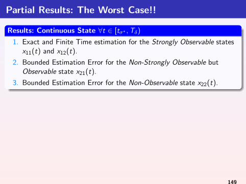
Partial Results: The Worst Case!!
Results: Continuous State ∀t ∈ [tσ∗ ,Tδ)
1. Exact and Finite Time estimation for the Strongly Observable statesx11(t) and x12(t).
2. Bounded Estimation Error for the Non-Strongly Observable butObservable state x21(t).
3. Bounded Estimation Error for the Non-Observable state x22(t).
149
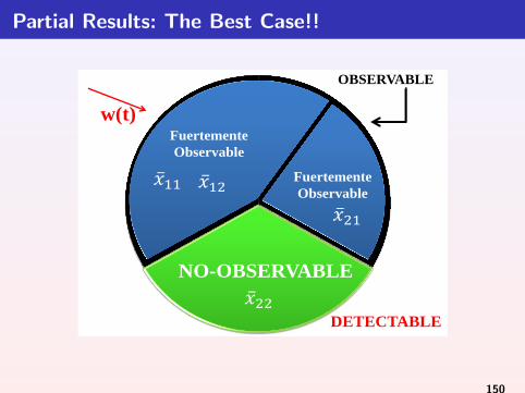
Partial Results: The Best Case!!
OBSERVABLE
𝑥 11 𝑥 12
𝑥 21
𝑥 22 DETECTABLE
w(t)
Fuertemente
Observable
Fuertemente
Observable
NO-OBSERVABLE
150
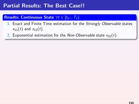
Partial Results: The Best Case!!
Results: Continuous State ∀t ∈ [tσ∗ ,Tδ)
1. Exact and Finite Time estimation for the Strongly Observable statesx11(t) and x12(t).
2. Exponential estimation for the Non-Observable state x22(t).
150
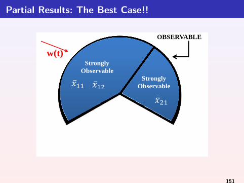
Partial Results: The Best Case!!
OBSERVABLE
𝑥 11 𝑥 12
𝑥 21
w(t) Strongly
Observable
Strongly
Observable
151
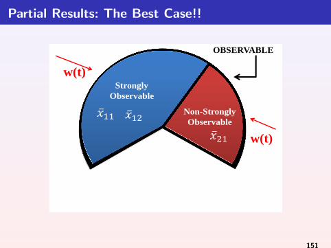
Partial Results: The Best Case!!
OBSERVABLE
𝑥 11 𝑥 12
𝑥 21
w(t)
w(t)
Non-Strongly
Observable
Strongly
Observable
151
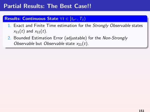
Partial Results: The Best Case!!
Results: Continuous State ∀t ∈ [tσ∗ ,Tδ)
1. Exact and Finite Time estimation for the Strongly Observable statesx11(t) and x12(t).
2. Bounded Estimation Error (adjustable) for the Non-StronglyObservable but Observable state x21(t).
151
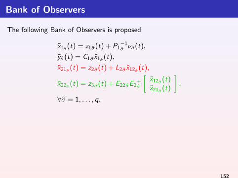
Bank of Observers
The following Bank of Observers is proposed
x1σ(t) = z1σ(t) + P1−1σ νσ(t),
yσ(t) = C1σ x1σ(t),
x21σ(t) = z2σ(t) + L2σ x12σ(t),
x22σ(t) = z3σ(t) + E22σE2+σ
[x12σ(t)x21σ(t)
],
∀σ = 1, . . . , q,
Assumptions: Discrete State
3. Known initial Discrete State, i.e. σ(0) = σ(0) = σ∗ known.
4. Strictly positive Dwell time, such that tσ∗ < Tδ.
5. The eigenvalues of A44σ∗ and the i.c. x(0), allow to satisfy tσ∗ < t1.
152
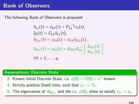

Discrete State Estimation
AUTONOMOUS SWITCHINGS
Consider the discrete state observer
σ(t) =
1, ∀x(t) | Hx(t) ∈ H1,2, ∀x(t) | Hx(t) ∈ H2,...q, ∀x(t) | Hx(t) ∈ Hq,
Observability Matrix
Qσ =[
HT , (HAσ)T , · · · , (HAn−1σ )T
]T.
V∗σ ⊂ ker(Qσ), ∀σ ∈ Q = {1, . . . , q} .
⇒ σ(t) is estimated Exactly and in Finite Time.
153
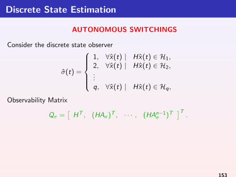
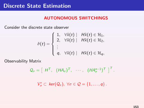
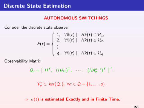
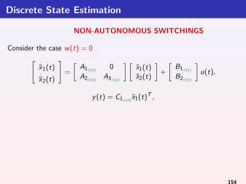
Discrete State Estimation
NON-AUTONOMOUS SWITCHINGS
Consider the case w(t) = 0[ ·x1(t)·x2(t)
]=
[A1σ(t)
0
A2σ(t)A3σ(t)
] [x1(t)x2(t)
]+
[B1σ(t)
B2σ(t)
]u(t),
y(t) = C1σ(t)x1(t)T ,
Assumptions: Discrete State
5a. The eigenvalues of A3σ∗ and the i.c. x(0), allow to satisfy tσ∗ < t1.
6.A1i 6= A1j ∨ B1i 6= B1j , ∀i 6= j , ∀i , j ∈ Q.
154
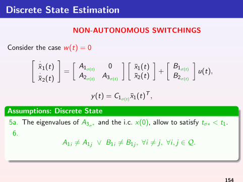
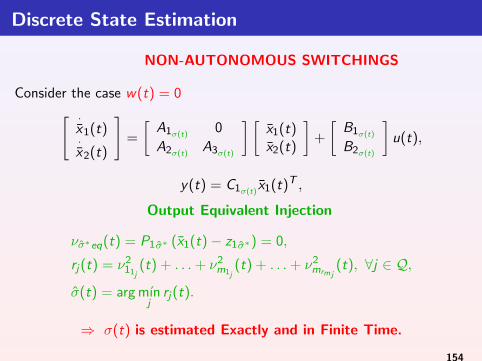
Discrete State Estimation
NON-AUTONOMOUS SWITCHINGS
Consider the case w(t) = 0[ ·x1(t)·x2(t)
]=
[A1σ(t)
0
A2σ(t)A3σ(t)
] [x1(t)x2(t)
]+
[B1σ(t)
B2σ(t)
]u(t),
y(t) = C1σ(t)x1(t)T ,
Output Equivalent Injection
νσ∗eq(t) = P1σ∗ (x1(t)− z1σ∗) = 0,
rj (t) = ν211j
(t) + . . .+ ν2m1j
(t) + . . .+ ν2mrmj
(t), ∀j ∈ Q,
σ(t) = arg mınj
rj (t).
⇒ σ(t) is estimated Exactly and in Finite Time.
154
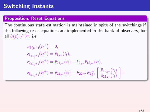
Switching Instants
Proposition: Reset Equations
The continuous state estimation is maintained in spite of the switchings ifthe following reset equations are implemented in the bank of observers, forall σ(t) 6= σ∗, i.e.
νσ(ti+)(ti
+) = 0,
z1σ(ti+)
(ti+) = x1σ∗ (ti ),
z2σ(ti+)
(ti+) = x21σ∗ (ti )− L2σ∗ x12σ∗ (ti ),
z3σ(ti+)
(ti+) = x22σ∗ (ti )− E22σ∗E2
+σ∗
[x12σ∗ (ti )x21σ∗ (ti )
].
155
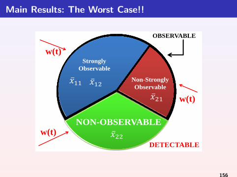
Main Results: The Worst Case!!
OBSERVABLE
𝑥 11 𝑥 12
𝑥 21
𝑥 22 DETECTABLE
w(t)
w(t)
w(t)
NON-OBSERVABLE
Non-Strongly
Observable
Strongly
Observable
156
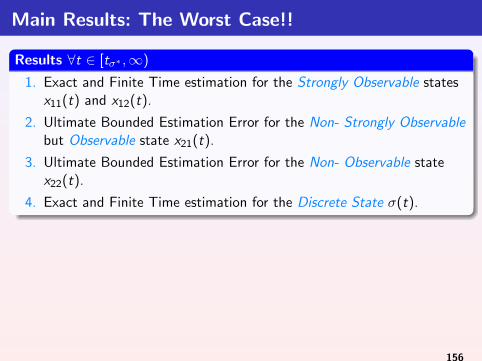
Main Results: The Worst Case!!
Results ∀t ∈ [tσ∗ ,∞)
1. Exact and Finite Time estimation for the Strongly Observable statesx11(t) and x12(t).
2. Ultimate Bounded Estimation Error for the Non- Strongly Observablebut Observable state x21(t).
3. Ultimate Bounded Estimation Error for the Non- Observable statex22(t).
4. Exact and Finite Time estimation for the Discrete State σ(t).
156

HOSM observers for switched systems
Remarks
the HOSM differentiator needs a finite time to converge;
therefore the switching system requires to have a positive dwell-time ;
nevertheless, this is not sufficient: its convergence time grows withinitial differentiator error;
Conclusions
to apply HOSM observers for switching systems, a uniform HOSMdifferentiator is required;
a first order uniform robust exact differentiator [Cruz et.al. IEEE TAC2011];
arbitrary order uniform robust exact differentiator [Angulo et. al. Aut2013].
157

Outline
1 Conventional Sliding Mode Observers
2 Higher Order Sliding Mode Observers
3 Cascaded HOSM Observers for Linear systems with unknown inputs
4 Super-twisting based Observers for Mechanical Systems
5 HOSM based Observers for Nonlinear Systems
6 Output-feedback finite-time stabilization of disturbed LTI systems
7 Unknown input identification
8 Parameter Identification
9 Output-based stabilization of disturbed systems
10 Switched Systems
11 Fault detectionFault detection using multi-model approach
158
Outline
11 Fault detectionFault detection using multi-model approach
159
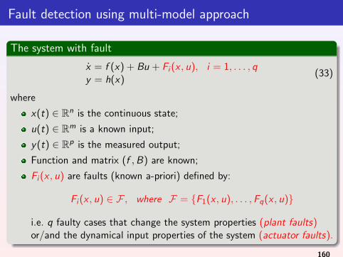
Fault detection using multi-model approach
The system with fault
x = f (x) + Bu + Fi (x , u), i = 1, . . . , qy = h(x)
(33)
where
x(t) ∈ Rn is the continuous state;
u(t) ∈ Rm is a known input;
y(t) ∈ Rp is the measured output;
Function and matrix (f ,B) are known;
Fi (x , u) are faults (known a-priori) defined by:
Fi (x , u) ∈ F , where F = {F1(x , u), . . . ,Fq(x , u)}
i.e. q faulty cases that change the system properties (plant faults)or/and the dynamical input properties of the system (actuator faults).
160
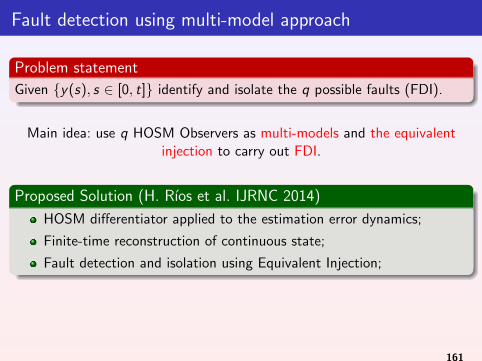
Fault detection using multi-model approach
Problem statement
Given {y(s), s ∈ [0, t]} identify and isolate the q possible faults (FDI).
Main idea: use q HOSM Observers as multi-models and the equivalentinjection to carry out FDI.
Proposed Solution (H. Rıos et al. IJRNC 2014)
HOSM differentiator applied to the estimation error dynamics;
Finite-time reconstruction of continuous state;
Fault detection and isolation using Equivalent Injection;
161
Conclusions
HOSM Observersprovide theoretically exact observation and unknown inputs and faultestimation under sufficient and necessary conditions of the strongobservability/ detectability of states or unknown inputs or faults;
provide best possible approximation w.r.t. discretization step and/orbounded deterministic noises:
can ensure prescribed time convergence independent from any initialconditions.
162

163
References
REFERENCES
Y. Shtessel, C. Edwards , L. Fridman, A. Levant. Sliding Mode Controland Observation, Series: Control Engineering, Birkhauser: Basel, 2014.
L. Fridman, A. Levant and J. Davila Robust Exact Observation andIdentification via High-Order Sliding Modes, in: The Industrial ElectronicsHandbook Volume; Control and Mechatronics, Editors: BogdanWilamowski, J. David Irwin. CRC Press, Taylor & Francis Inc., 2011,ISBN: 9781439802878.
http://verona.fi-p.unam.mx/ lfridman/
164


![On sliding mode observers for systems with unknown inputs · 2020-03-09 · The concept of sliding mode control [12, 27, 33] has been extended to the problem of state estimation by](https://img.pdfslide.net/doc/110x75/5e81557108dd1f50e30f7d29/on-sliding-mode-observers-for-systems-with-unknown-inputs-2020-03-09-the-concept.jpg)