Embed Size (px)
Citation preview
UNIT -1
COMPUTER INTEGRATED MANUFACTURING SYSTEMS
1. INTRODUCTION
Computer Integrated Manufacturing (CIM) encompasses the entire range of product
development and manufacturing activities with all the functions being carried out with the
help of dedicated software packages. The data required for various functions are passed from
one application software to another in a seamless manner. For example, the product data is
created during design. This data has to be transferred from the modeling software to
manufacturing software without any loss of data. CIM uses a common database
wherever feasible and communication technologies to integrate design, manufacturing and
associated business functions that combine the automated segments of a factory or a
manufacturing facility. CIM reduces the human component of manufacturing and thereby
relieves the process of its slow, expensive and error-prone component. CIM stands for a holistic
and methodological approach to the activities of the manufacturing enterprise in order to
achieve vast improvement in its performance.
This methodological approach is applied to all activities from the design of the product to
customer support in an integrated way, using various methods, means and techniques in
order to achieve production improvement, cost reduction, fulfillment of scheduled
delivery dates, quality improvement and total flexibility in the manufacturing system. CIM
requires all those associated with a company to involve totally in the process of product
development and manufacture. In such a holistic approach, economic, social and human
aspects have the same importance as technical aspects. CIM also encompasses the whole lot
of enabling technologies including total quality management, business process
reengineering, concurrent engineering, workflow automation, enterprise resource
planning and flexible manufacturing.
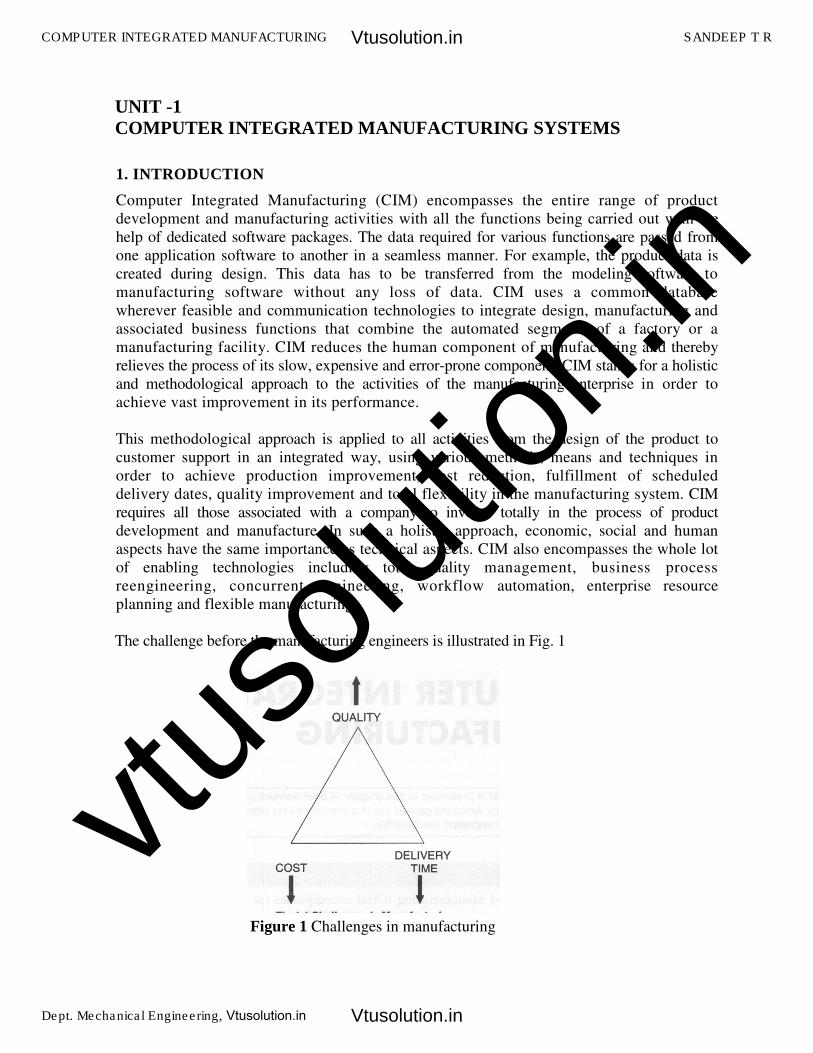
The challenge before the manufacturing engineers is illustrated in Fig. 1
�
�
�
�
�
�
�
�
�
�
�
�
�
�Figure 1 Challenges in manufacturing
COMPUTER INTEGRATED MANUFACTURING SANDEEP T R
Dept. Mechanical Engineering, Vtusolution.in
Vtusolution.in
Vtusolution.in
vtuso
lution
.in
�
Manufacturing industries strive to reduce the cost of the product continuously to remain competitive
in the face of global competition. In addition, there is the need to improve the quality and
performance levels on a continuing basis. Another important requirement is on time delivery. In
the context of global outsourcing and long supply chains cutting across several international
borders, the task of continuously reducing delivery times is really an arduous task. CIM has
several software tools to address the above needs.
Manufacturing engineers are required to achieve the following objectives to be competitive
in a global context.
• Reduction in inventory
• Lower the cost of the product
• Reduce waste
• Improve quality
• Increase flexibility in manufacturing to achieve immediate and rapid response
to:
• Product changes
• Production changes
• Process change
• Equipment change
• Change of personnel
CIM technology is an enabling technology to meet the above challenges to the
manufacturing.
2. EVOLUTION OF COMPUTER INTEGRATED MANUFACTURING
Computer Integrated Manufacturing (CIM) is considered a natural evolution of the
technology of CAD/CAM which by itself evolved by the integration of CAD and CAM.
Massachusetts Institute of Technology (MIT, USA) is credited with pioneering the
development in both CAD and CAM. The need to meet the design and manufacturing
requirements of aerospace industries after the Second World War necessitated the
development these technologies. The manufacturing technology available during late 40's and
early 50's could not meet the design and manufacturing challenges arising out of the need to
develop sophisticated aircraft and satellite launch vehicles. This prompted the US Air Force to
approach MIT to develop suitable control systems, drives and programming techniques for
machine tools using electronic control.
�
�
�
�
�
COMPUTER INTEGRATED MANUFACTURING SANDEEP T R
Dept. Mechanical Engineering, Vtusolution.in
Vtusolution.in
Vtusolution.in
vtuso
lution
.in
The first major innovation in machine control is the Numerical Control (NC),
demonstrated at MIT in 1952. Early Numerical Control Systems were all basically hardwired
systems, since these were built with discrete systems or with later first generation integrated
chips. Early NC machines used paper tape as an input medium. Every NC machine was
fitted with a tape reader to read paper tape and transfer the program to the memory of the
machine tool block by block. Mainframe computers were used to control a group of NC
machines by mid 60's. This arrangement was then called Direct Numerical Control (DNC) as
the computer bypassed the tape reader to transfer the program data to the machine
controller. By late 60's mini computers were being commonly used to control NC machines. At
this stage NC became truly soft wired with the facilities of mass program storage, offline
editing and software logic control and processing. This development is called Computer
Numerical Control (CNC). Since 70's, numerical controllers are being designed around
microprocessors, resulting in compact CNC systems. A further development to this
technology is the distributed numerical control (also called DNC) in which processing of
NC program is carried out in different computers operating at different hierarchical levels -
typically from mainframe host computers to plant computers to the machine controller.
Today the CNC systems are built around powerful 32 bit and 64 bit microprocessors. PC
based systems are also becoming increasingly popular.
Manufacturing engineers also started using computers for such tasks like inventory
control, demand forecasting, production planning and control etc. CNC technology was
adapted in the development of co-ordinate measuring machine's (CMMs) which automated
inspection. Robots were introduced to automate several tasks like machine loading,
materials handling, welding, painting and assembly. All these developments led to the
evolution of flexible manufacturing cells and flexible manufacturing systems in late 70's.
Evolution of Computer Aided Design (CAD), on the other hand was to cater to the
geometric modeling needs of automobile and aeronautical industries. The developments in
computers, design workstations, graphic cards, display devices and graphic input and
output devices during the last ten years have been phenomenal. This coupled with the
development of operating system with graphic user interfaces and powerful interactive (user
friendly) software packages for modeling, drafting, analysis and optimization provides
the necessary tools to automate the design process.
CAD in fact owes its development to the APT language project at MIT in early 50's.
Several clones of APT were introduced in 80's to automatically develop NC codes from the
geometric model of the component. Now, one�can model, draft, analyze, simulate, modify,
optimize and create the NC code to manufacture a component and simulate the machining
operation sitting at a computer workstation.
If we review the manufacturing scenario during 80's we will find that the
manufacturing is characterized by a few islands of automation. In the case of design, the
task is well automated. In the case of manufacture, CNC machines, DNC systems, FMC,
FMS etc provide tightly controlled automation systems. Similarly computer control has been
implemented in several areas like manufacturing resource planning, accounting, sales,
marketing and purchase. Yet the full potential of computerization could not be obtained
COMPUTER INTEGRATED MANUFACTURING SANDEEP T R
Dept. Mechanical Engineering, Vtusolution.in
Vtusolution.in
Vtusolution.in
vtuso
lution
.in
unless all the segments of manufacturing are integrated, permitting the transfer of data
across various functional modules. This realization led to the concept of computer integrated
manufacturing. Thus the implementation of CIM required the development of whole lot
of computer technologies related to hardware and software.
3. CIM HARDWARE AND CIM SOFTWARE
CIM Hardware comprises the following:
i. Manufacturing equipment such as CNC machines or computerized work centers,
robotic work cells, DNC/FMS systems, work handling and tool handling devices,
storage devices, sensors, shop floor data collection devices, inspection machines etc.
ii. Computers, controllers, CAD/CAM systems, workstations / terminals, data entry
terminals, bar code readers, RFID tags, printers, plotters and other peripheral
devices, modems, cables, connectors etc.,
CIM software comprises computer programmes to carry out the following functions:
• Management Information System
• Sales
• Marketing
• Finance
• Database Management
• Modeling and Design
• Analysis
• Simulation
• Communications
• Monitoring
• Production Control
• Manufacturing Area Control
• Job Tracking
• Inventory Control
• Shop Floor Data Collection
• Order Entry
• Materials Handling
• Device Drivers
• Process Planning
• Manufacturing Facilities Planning
• Work Flow Automation
• Business Process Engineering
• Network Management
• Quality Management
COMPUTER INTEGRATED MANUFACTURING SANDEEP T R
Dept. Mechanical Engineering, Vtusolution.in
Vtusolution.in
Vtusolution.in
vtuso
lution
.in
4. NATURE AND ROLE OF THE ELEMENTS OF CIM SYSTEM
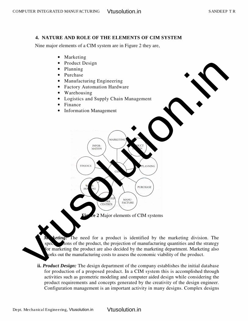
Nine major elements of a CIM system are in Figure 2 they are,
• Marketing
• Product Design
• Planning
• Purchase
• Manufacturing Engineering
• Factory Automation Hardware
• Warehousing
• Logistics and Supply Chain Management
• Finance
• Information Management
�
�
�
�
�
�
��
�
�
�
�
i. Marketing: The need for a product is identified by the marketing division. The
specifications of the product, the projection of manufacturing quantities and the strategy
for marketing the product are also decided by the marketing department. Marketing also
works out the manufacturing costs to assess the economic viability of the product.
ii. Product Design: The design department of the company establishes the initial database
for production of a proposed product. In a CIM system this is accomplished through
activities such as geometric modeling and computer aided design while considering the
product requirements and concepts generated by the creativity of the design engineer.
Configuration management is an important activity in many designs. Complex designs
Figure 2 Major elements of CIM systems
COMPUTER INTEGRATED MANUFACTURING SANDEEP T R
Dept. Mechanical Engineering, Vtusolution.in
Vtusolution.in
Vtusolution.in
vtuso
lution
.in

are usually carried out by several teams working simultaneously, located often in
different parts of the world. The design process is constrained by the costs that will be
incurred in actual production and by the capabilities of the available production
equipment and processes. The design process creates the database required to
manufacture the part.
iii. Planning: The planning department takes the database established by the design
department and enriches it with production data and information to produce a plan
for the production of the product. Planning involves several subsystems dealing with
materials, facility, process, tools, manpower, capacity, scheduling, outsourcing,
assembly, inspection, logistics etc. In a CIM system, this planning process should be
constrained by the production costs and by the production equipment and process
capability, in order to generate an optimized plan.
iv. Purchase: The purchase departments is responsible for placing the purchase orders
and follow up, ensure quality in the production process of the vendor, receive the
items, arrange for inspection and supply the items to the stores or arrange timely
delivery depending on the production schedule for eventual supply to manufacture and
assembly.
v. Manufacturing Engineering: Manufacturing Engineering is the activity of carrying out the
production of the product, involving further enrichment of the database with
performance data and information about the production equipment and processes. In
CIM, this requires activities like CNC programming, simulation and computer aided
scheduling of the production activity. This should include online dynamic scheduling
and control based on the real time performance of the equipment and processes to
assure continuous production activity. Often, the need to meet fluctuating market
demand requires the manufacturing system flexible and agile.
vi. Factory Automation Hardware: Factory automation equipment further enriches the
database with equipment and process data, resident either in the operator or the
equipment to carry out the production process. In CIM system this consists of
computer controlled process machinery such as CNC machine tools, flexible
manufacturing systems (FMS), Computer controlled robots, material handling systems,
computer controlled assembly systems, flexibly automated inspection systems and so on.
vii. Warehousing: Warehousing is the function involving storage and retrieval of raw
materials, components, finished goods as well as shipment of items. In today's complex
outsourcing scenario and the need for just-in-time supply of components and
subsystems, logistics and supply chain management assume great importance.
viii. Finance: Finance deals with the resources pertaining to money. Planning of
investment, working capital, and cash flow control, realization of receipts,
accounting and allocation of funds are the major tasks of the finance departments.
COMPUTER INTEGRATED MANUFACTURING SANDEEP T R
Dept. Mechanical Engineering, Vtusolution.in
Vtusolution.in
Vtusolution.in
vtuso
lution
.in
ix. Information Management: Information Management is perhaps one of the crucial tasks in
CIM. This involves master production scheduling, database management, communication,
manufacturing systems integration and management information systems.
�
�
Definition of CIM
Joel Goldhar, Dean, Illinois Institute of Technology gives CIM as a computer system in which
the peripherals are robots, machine tools and other processing equipment.
Dan Appleton, President, DACOM, Inc. defines CIM is a management philosophy, not a turnkey
product.
Jack Conaway, CIM Marketing manager, DEC, defines CIM is nothing but a data management
and networking problem.
The computer and automated systems association of the society of Manufacturing Engineers
(CASA/SEM) defines CIM is the integration of total manufacturing enterprise by using
integrated systems and data communication coupled with new managerial philosophies that
improve organizational and personnel efficiency.
CIM is recognized as Islands of Automation. They are
1. CAD/CAM/CAE/GT
2. Manufacturing Planning and Control.
3. Factory Automation
4. General Business Management
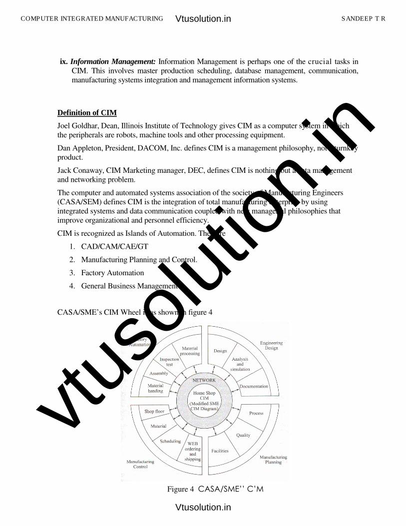
CASA/SME’s CIM Wheel is as shown in figure 4
�
�
�
�
�
�
�
�
�
�
�
COMPUTER INTEGRATED MANUFACTURING SANDEEP T R
Figure 4 ���������������
���
Dept. Mechanical Engineering, Vtusolution.in
Vtusolution.in
Vtusolution.in
vtuso
lution
.in
�
Conceptual model of manufacturing
The computer has had and continues to have a dramatic impact on the development of
production automation technologies. Nearly all modern production systems are imple-
mented today using computer systems. The term computer integrated manufacturing
(CIM) has been coined to denote the pervasive use of computers to design the products,
plan the production, control the operations, and perform the various business related
functions needed in a manufacturing firm. CAD/CAM (computer-aided design and com-
puter-aided manufacturing) is another term that is used almost synonymously with CIM.
Let us attempt to define the relationship between automation and CIM by developing a
conceptual model of manufacturing. In a manufacturing firm, the physical activities
related to production that take place in the factory can be distinguished from the infor-
mation-processing activities, such as product design and production planning, that usually
occur in an office environment. The physical activities include all of the manufacturing
processing, assembly, material handling, and inspections that are performed on the prod-
uct. These operations come in direct contact with the product during manufacture. They
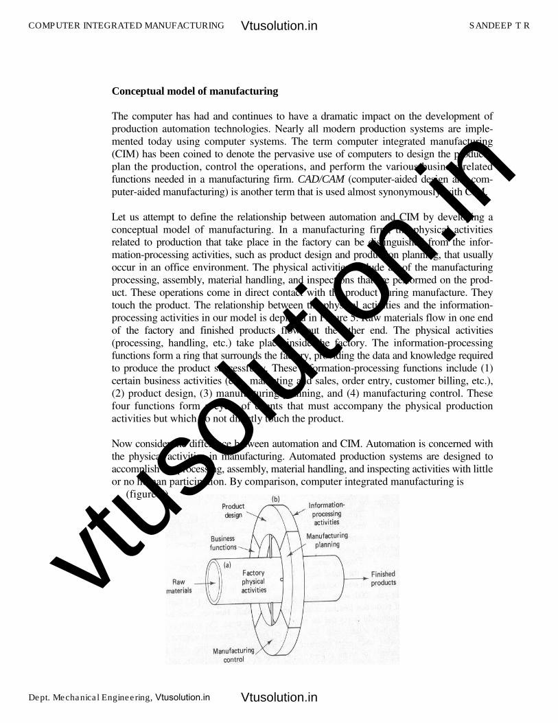
touch the product. The relationship between the physical activities and the information-
processing activities in our model is depicted in Figure 5. Raw materials flow in one end
of the factory and finished products flow out the other end. The physical activities
(processing, handling, etc.) take place inside the factory. The information-processing
functions form a ring that surrounds the factory, providing the data and knowledge required
to produce the product successfully. These information-processing functions include (1)
certain business activities (e.g., marketing and sales, order entry, customer billing, etc.),
(2) product design, (3) manufacturing planning, and (4) manufacturing control. These
four functions form a cycle of events that must accompany the physical production
activities but which do not directly touch the product.
Now consider the difference between automation and CIM. Automation is concerned with
the physical activities in manufacturing. Automated production systems are designed to
accomplish the processing, assembly, material handling, and inspecting activities with little
or no human participation. By comparison, computer integrated manufacturing is
(figure 5)
�
�
�
�
�
�
�
�
�
�
�
COMPUTER INTEGRATED MANUFACTURING SANDEEP T R
Dept. Mechanical Engineering, Vtusolution.in
Vtusolution.in
Vtusolution.in
vtuso
lution
.in
�
�
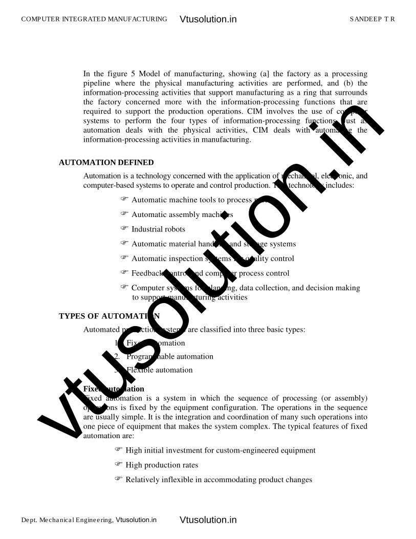
In the figure 5 Model of manufacturing, showing (a] the factory as a processing
pipeline where the physical manufacturing activities are performed, and (b) the
information-processing activities that support manufacturing as a ring that surrounds
the factory concerned more with the information-processing functions that are
required to support the production operations. CIM involves the use of computer
systems to perform the four types of information-processing functions. Just as
automation deals with the physical activities, CIM deals with automating the
information-processing activities in manufacturing.
AUTOMATION DEFINED
Automation is a technology concerned with the application of mechanical, electronic, and
computer-based systems to operate and control production. This technology includes:
� Automatic machine tools to process parts
� Automatic assembly machines
� Industrial robots
� Automatic material handling and storage systems
� Automatic inspection systems for quality control
� Feedback control and computer process control
� Computer systems for planning, data collection, and decision making
to support manufacturing activities
TYPES OF AUTOMATION
Automated production systems are classified into three basic types:
1. Fixed automation
2. Programmable automation
3. Flexible automation
Fixed automation
Fixed automation is a system in which the sequence of processing (or assembly)
operations is fixed by the equipment configuration. The operations in the sequence
are usually simple. It is the integration and coordination of many such operations into
one piece of equipment that makes the system complex. The typical features of fixed
automation are:
� High initial investment for custom-engineered equipment
� High production rates
� Relatively inflexible in accommodating product changes
COMPUTER INTEGRATED MANUFACTURING SANDEEP T R
Dept. Mechanical Engineering, Vtusolution.in
Vtusolution.in
Vtusolution.in
vtuso
lution
.in
The economic justification for fixed automation is found in products with very high
demand rates and volumes. The high initial cost of the equipment can be spread over a
very large number of units, thus making the unit cost attractive compared to alternative
methods of production.
Programmable automation
In programmable automation, the production equipment is designed with the ca-
pability to change the sequence of operations to accommodate different product
configurations. The operation sequence is controlled by a program, which is a set of
instructions coded so that the system can read and interpret them. New programs can
be prepared and entered into the equipment lo produce new products. Some of the
features that characterize programmable automation include:
� High investment in general-purpose equipment
� Low production rates relative to fixed automation
� Flexibility to deal with changes in product configuration
� Most suitable for batch production
Automated production systems that are programmable are used in low and medium-
volume production. The parts or products are typically made in batches. To produce each
new batch of a different product, the system must be reprogrammed with the set of
machine instructions that correspond to the new product. The physical setup of the machine
must also be changed over: Tools must be loaded, fixtures must be attached to the machine
table, and the required machine settings must be entered. This changeover procedure
takes time. Consequently, the typical cycle for a given product includes a period during
which the setup and reprogramming takes place, followed by a period in which the batch
is produced.
Flexible automation
Flexible automation is an extension of programmable automation. The concept of flexible
automation has developed only over the last 15 to 20 years, and the principles are still
evolving. A flexible automated system is one that is capable of producing a variety of
products (or parts) with virtually no time lost for changeovers from one product to the
next. There is no production time lost while reprogramming the system and altering the
physical setup (tooling, fixtures and machine settings). Consequently, the system can
produce various combinations and schedules of products, instead of requiring that they
be made in separate batches.
COMPUTER INTEGRATED MANUFACTURING SANDEEP T R
Dept. Mechanical Engineering, Vtusolution.in
Vtusolution.in
Vtusolution.in
vtuso
lution
.in
The features of flexible automation can be summarized as follows:
� High investment for a custom-engineered system
� Continuous production of variable mixtures of products
� Medium production rates
� Flexibility to deal with product design variations
The essential features that distinguish flexible automation from programmable au-
tomation are (1) the capacity to change part programs with no lost production time, and
(2) the capability to change over the physical setup, again with no lost production time.
These features allow the automated production system to continue production without the
downtime between batches that is characteristic of programmable automation. Changing
the part programs is generally accomplished by preparing the programs off-line on a
computer system and electronically transmitting the programs to the automated production
system. Therefore, the time required to do the programming for the next job does not
interrupt production on the current job. Advances in computer systems technology are
largely responsible for this programming capability in flexible automation. Changing the
physical setup between parts is accomplished by making the changeover off-line and then
moving it into place simultaneously as the next part comes into position for processing.
The use of pallet fixtures that hold the parts and transfer into position at the workplace
is one way of implementing this approach. For these approaches to be successful, the
variety of parts that can be made on a flexible automated production system is usually
more limited than a system controlled by programmable automation.
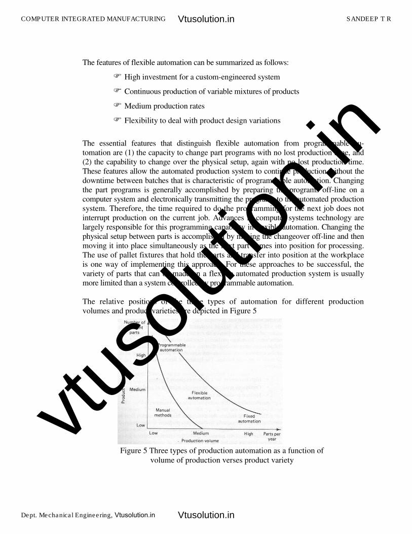
The relative positions of the three types of automation for different production
volumes and product varieties are depicted in Figure 5
�
�
�
�
�
�
�
�
�
�
�
Figure 5 Three types of production automation as a function of
volume of production verses product variety
COMPUTER INTEGRATED MANUFACTURING SANDEEP T R
Dept. Mechanical Engineering, Vtusolution.in
Vtusolution.in
Vtusolution.in
vtuso
lution
.in
�
REASONS FOR AUTOMATING
The important reasons for automating include the following:
1. Increased productivity: Automation of manufacturing operations holds the
promise of increasing the productivity of labor. This means greater output per
hour of labor input. Higher production rates (output per hour) are achieved with
automation than with the corresponding manual operations.
2. High cost of labor: The trend in the industrialized societies of the world has
been toward ever-increasing labor costs. As a result, higher investment in
automated equipment has become economically justifiable to replace manual
operations. The high cost of labor is forcing business leaders to substitute
machines for human labor. Because machines can produce at higher rates of
output, the use of automation results in a lower cost per unit of product.
3. Labor shortages: In many advanced nations there has been a general shortage of
labor. Labor shortages also stimulate the development of automation as a
substitute for labor.
4. Trend of labor toward the service sector: This trend has been especially
prevalent in the advanced countries. First around 1986, the proportion of the
work force employed in manufacturing stands at about 20%. In 1947, this
percentage was 30%. By the year 2000, some estimates put the figure as low as
2%, certainly, automation of production jobs has caused some of this shift.
The growth of government employment at the federal, state, and local levels has
consumed a certain share of the labor market which might otherwise have gone
into manufacturing. Also, there has been a tendency for people to view factory
work as tedious, demeaning, and dirty. This view has caused them to seek
employment in the service sector of the economy.
5. Safe: By automating the operation and transferring the operator from an active
participation to a supervisory role, work is made safer. The safety and physical
well-being of the worker has become a national objective with the enactment
of the Occupational. Safety and Health Act of 1970 (OSHA). It has also
provided an impetus for automation.
6. High cost of raw materials: The high cost of raw materials in manufacturing
results in the need for greater efficiency in using these materials. The reduction
of scrap is one of the benefits of automation.
7. Improved product quality: Automated operations not only produce parts at
faster rates than do their manual counterparts, but they produce parts with
greater consistency and conformity to quality specifications.
8. Reduced manufacturing lead time: For reasons that we shall examine in sub
sequent chapters, automation allows the manufacturer to reduce the time between
customer order and product delivery. This gives the manufacturer a
competitive advantage in promoting good customer service.
COMPUTER INTEGRATED MANUFACTURING SANDEEP T R
Dept. Mechanical Engineering, Vtusolution.in
Vtusolution.in
Vtusolution.in
vtuso
lution
.in
9. Reduction of in-process inventory: Holding large inventories of work-in-process
represents a significant cost to the manufacturer because it ties up capital. In-
process inventory is of no value. It serves none of the purposes of raw materials
stock or finished product inventory. Accordingly, it is to the manufacturer's
advantage to reduce work-in- progress to a minimum. Automation tends to
accomplish this goal by reducing the time a workpart spends in the factory.
10. High cost of not automating: A significant competitive advantage is gained by
automating a manufacturing plant. The advantage cannot easily be demonstrated
on a company's project authorization form. The benefits of automation often show
up in intangible and unexpected ways, such as improved quality, higher sales,
better labor relations, and better company image. Companies that do not automate
are likely to find themselves at a competitive disadvantage with their customers,
their employees, and the general public.
All of these factors act together to make production automation a feasible and
attractive alternative to manual methods of manufacture.
�
TYPES OF PRODUCTION
Another way of classifying production activity is according to the quantity of product
made. In this classification, there are three types of production:
1. Job shop production
2. Batch production
3. Mass production
1.Job shop production. The distinguishing feature of job shop production is low volume.
The manufacturing lot sizes are small, often one of a kind. Job shop production is
commonly used to meet specific customer orders, and there is a great variety in the type
of work the plant must do. Therefore, the production equipment must be flexible and
general-purpose to allow for this variety of work. Also, the skill level of job shop workers
must be relatively high so that they can perform a range of different work assignments.
Examples of products manufactured in a job shop include space vehicles, aircraft, machine
tools, special tools and equipment, and prototypes of future products. Construction work
and shipbuilding are not normally identified with the job shop category, even though the
quantities are in the appropriate range. Although these two activities involve the
transformation of raw materials into finished products, the work is not performed in a
factory.
COMPUTER INTEGRATED MANUFACTURING SANDEEP T R
Dept. Mechanical Engineering, Vtusolution.in
Vtusolution.in
Vtusolution.in
vtuso
lution
.in
2. Batch production: This category involves the manufacture of medium-sized lots of the
same item or product. The lots may be produced only once, or they may be produced at
regular intervals. The purpose of batch production is often to satisfy continuous customer
demand for an item. However, the plant is capable of a production rate that exceeds the
demand rate. Therefore, the shop produces to build up an inventory of the item. Then it
changes over to other orders. When the stock of the first item becomes depleted, production
is repeated to build up the inventory again. The manufacturing equipment used in batch
production is general-purpose but designed for higher rates of production. Examples of
items made in batch-type shops include industrial equipment, furniture, textbooks, and
component parts for many assembled consumer products (household appliances, lawn
mowers, etc.). Batch production plants include machine shops, casting foundries, plastic
molding factories, and press working shops. Some types of chemical plants are also in
this general category.
3. Mass production: This is the continuous specialized manufacture of identical products.
Mass production is characterized by very high production rates, equipment that is
completely dedicated to the manufacture of a particular product, and very high demand rates
for the product. Not only is the equipment dedicated to one product, but the entire plant is
often designed for the exclusive purpose of producing the particular product. The
equipment is special-purpose rather than general-purpose. The investment in machines
and specialized tooling is high. In a sense, the production skill has been transferred from
the operator to the machine. Consequently, the skill level of labor in a mass production
plant tends to be lower than in a batch plant or job shop.
2.3 FUNCTIONS IN MANUFACTURING
For any of the three types of production, there are certain basic functions that must be
carried out to convert raw materials into finished product. For a firm engaged in making
discrete products, the functions are:
1. Processing
2. Assembly
3. Material handling and storage
4. Inspection and test
5. Control
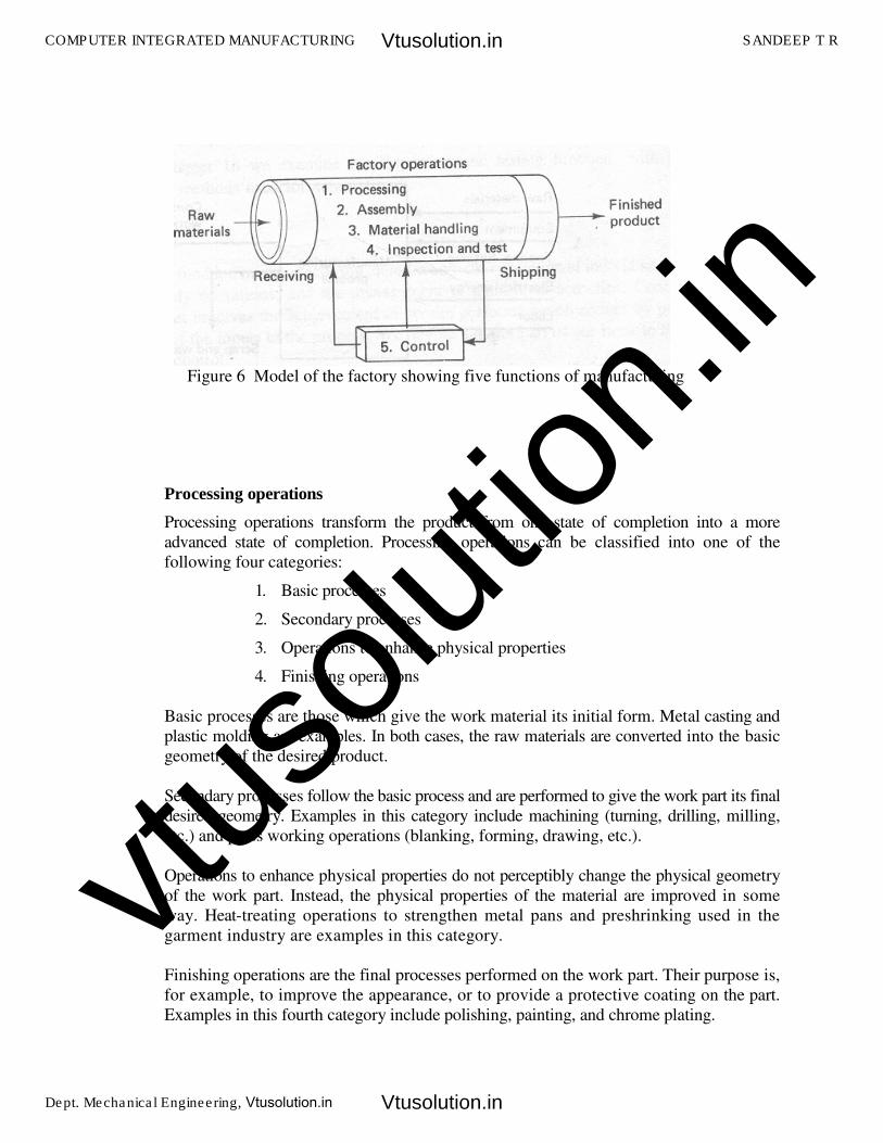
The first four of these functions are the physical activities that "touch" the product as it is
being made. Processing and assembly are operations that add value to the product. The third
and fourth functions must be performed in a manufacturing plant, but they do not add value
to the product. The Figure 6, shows the model of the functions of manufacturing in factory .
COMPUTER INTEGRATED MANUFACTURING SANDEEP T R
Dept. Mechanical Engineering, Vtusolution.in
Vtusolution.in
Vtusolution.in
vtuso
lution
.in
�
�
�
�
�
�
�
�
�
�
�
�
�
�
�
�
Processing operations
Processing operations transform the product from one state of completion into a more
advanced state of completion. Processing operations can be classified into one of the
following four categories:
1. Basic processes
2. Secondary processes
3. Operations to enhance physical properties
4. Finishing operations
Basic processes are those which give the work material its initial form. Metal casting and
plastic molding are examples. In both cases, the raw materials are converted into the basic
geometry of the desired product.
Secondary processes follow the basic process and are performed to give the work part its final
desired geometry. Examples in this category include machining (turning, drilling, milling,
etc.) and press working operations (blanking, forming, drawing, etc.).
Operations to enhance physical properties do not perceptibly change the physical geometry
of the work part. Instead, the physical properties of the material are improved in some
way. Heat-treating operations to strengthen metal pans and preshrinking used in the
garment industry are examples in this category.
Finishing operations are the final processes performed on the work part. Their purpose is,
for example, to improve the appearance, or to provide a protective coating on the part.
Examples in this fourth category include polishing, painting, and chrome plating.
Figure 6 Model of the factory showing five functions of manufacturing
COMPUTER INTEGRATED MANUFACTURING SANDEEP T R
Dept. Mechanical Engineering, Vtusolution.in
Vtusolution.in
Vtusolution.in
vtuso
lution
.in
Figure 6 presents an input/output model of a typical processing operation in
manufacturing. Most manufacturing processes require five inputs:
1. Raw materials
2. Equipment
3. Tooling, fixtures
4. Energy (electrical energy)
5. Labor
Assembly operations
Assembly and joining processes constitute the second major type of manufacturing op-
eration. In assembly, the distinguishing feature is that two or more separate components are
joined together. Included in this category are mechanical fastening operations, which make
use of screws, nuts, rivets, and so on, and joining processes, such as welding, brazing,
and soldering. In the fabrication of a product, the assembly operations follow the
processing operations.
Material handling and storage
A means of moving and storing materials between the processing and assembly operations
must be provided. In most manufacturing plants, materials spend more time being moved
and stored than being processed. In some cases, the majority of the labor cost in the
factory is consumed in handling, moving, and storing materials. It is important that this
function be carried out as efficiently as possible.
Inspection and testing
Inspection and testing are generally considered part of quality control. The purpose of
inspection is to determine whether the manufactured product meets the established design
standards and specifications. For example, inspection examines whether the actual di-
mensions of a mechanical part are within the tolerances indicated on the engineering
drawing for the part and testing is generally concerned with the functional specifications of
the final product rather than the individual parts that go into the product.
Control
The control function in manufacturing includes both the regulation of individual processing
and assembly operations, and the management of plant-level activities. Control at the
process level involves the achievement of certain performance objectives by proper ma-
nipulation of the inputs to the process. Control at the plant level includes effective use of
labor, maintenance of the equipment, moving materials in the factory, shipping products
of good quality on schedule, and keeping plant operating costs at the minimum level
possible. The manufacturing control function at the plant level represents the major point
of intersection between the physical operations in the factory and the information-
processing activities that occur in production.
COMPUTER INTEGRATED MANUFACTURING SANDEEP T R
Dept. Mechanical Engineering, Vtusolution.in
Vtusolution.in
Vtusolution.in
vtuso
lution
.in
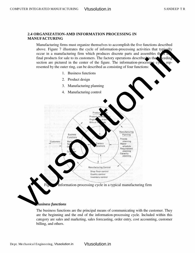
2.4 ORGANIZATION-AMD INFORMATION PROCESSING IN
MANUFACTURING
Manufacturing firms must organize themselves to accomplish the five functions described
above. Figure 7 illustrates the cycle of information-processing activities that typically
occur in a manufacturing firm which produces discrete parts and assembles them into
final products for sale to its customers. The factory operations described in the preceding
section are pictured in the center of the figure. The information-processing cycle, rep-
resented by the outer ring, can be described as consisting of four functions:
1. Business functions
2. Product design
3. Manufacturing planning
4. Manufacturing control
Business functions
The business functions are the principal means of communicating with the customer. They
are the beginning and the end of the information-processing cycle. Included within this
category are sales and marketing, sales forecasting, order entry, cost accounting, customer
billing, and others.
Figure 7 Information-processing cycle in a typical manufacturing firm
COMPUTER INTEGRATED MANUFACTURING SANDEEP T R
Dept. Mechanical Engineering, Vtusolution.in
Vtusolution.in
Vtusolution.in
vtuso
lution
.in
An order to produce a product will typically originate from the sales and marketing
department of the firm. The production order will be one of the following forms: (1) an
order to manufacture an item to the customer's�specifications, (2) a customer order to buy
one or more of the manufacturer's, proprietary products, or (3) an order based on a forecast
of future demand for a proprietary product.
Product design
If the product is to be manufactured to customer specifications, the design will have been
provided by the customer. The manufacturer's product design department will not be
involved.
If the product is proprietary, the manufacturing firm is responsible for its development and
design. The product design is documented by means of component drawings,
specifications, and a bill of materials that defines how many of each component goes into
the product.
Manufacturing planning
The information and documentation that constitute the design of the product flow into
the manufacturing planning function. The departments in the organization that perform
manufacturing planning include manufacturing engineering, industrial engineering, and
production planning and control.
As shown in Figure 7, the in formation-processing activities in manufacturing planning
include process planning, master scheduling, requirements planning, and capacity
planning. Process planning consists of determining the sequence of the individual
processing and assembly operations needed to produce the part. The document used to
specify the process sequence is called a route sheet. The route sheet lists the production
operations and associated machine tools for each component (and subassembly) of the
product. The manufacturing engineering and industrial engineering departments are
responsible for planning the processes and related manufacturing details. The
authorization to produce the product must be translated into the master schedule or master
production schedule. The master schedule is a listing of the products to be made,
when they are to be delivered, and in what quantities. Units of months are generally used
to specify the deliveries on the master schedule. Based on this schedule, the individual
components and subassemblies that make up each product must be planned. Raw
materials must be requisitioned, purchased parts must be ordered from suppliers, and all
of these items must be planned so that they are available when needed. This whole task is
called requirements planning or material requirements planning. In addition, the master
schedule must not list more quantities of products than the factory is capable of
producing with its given number of machines and workers each month. The production
quantity that the factory is capable of producing is referred to as the plant capacity. We
will define and discuss this term later in the chapter. Capacity planning is concerned
with planning the manpower and machine resources of the firm.
COMPUTER INTEGRATED MANUFACTURING SANDEEP T R
Dept. Mechanical Engineering, Vtusolution.in
Vtusolution.in
Vtusolution.in
vtuso
lution
.in
Manufacturing control
Manufacturing control is concerned with managing and controlling the physical
operations in the factory to implement the manufacturing plans.
Shop floor control is concerned with the problem of monitoring the progress of the product
as it is being processed, assembled, moved, and inspected in the factory. The sections of a
traditional production planning and control department that are involved in shop floor
control include scheduling, dispatching, and expediting. Production scheduling is concerned
with assigning start dates and due dates to the various parts (and products) that are to be
made in the factory. This requires that the parts be scheduled one by one through the
various production machines listed on the route sheet for each part. Based on the
production schedule, dispatching involves issuing the individual work orders to the
machine operators to accomplish the processing of the parts. The dispatching function is
performed in some plants by the shop foremen, in other plants by a person called the
dispatcher. Even with the best plans and schedules, things sometimes go wrong (e.g.,
machine breakdowns, improper tooling, parts delayed at the vendor). The expediter
compares the actual progress of a production order against the schedule. For orders that
fall behind, the expediter attempts to take the necessary corrective action to complete the
order on time.
Inventory control overlaps with shop floor control to some extent. Inventory control
attempts to strike a proper balance between the danger of too little inventory (with possible
stock-outs of materials) and the expense of having too much inventory. Shop floor control is
also concerned with inventory in the sense that the materials being processed in the
factory represent inventory (called work-in-process). The mission of quality control is to
assure that the quality of the product and its components meet the standards specified by the
product designer. To accomplish its mission, quality control depends on the inspection
activities performed in the factory at various times throughout the manufacture of the
product. Also, raw materials and components from outside sources must be inspected when
they are received. Final inspection and testing of the finished product is performed to
ensure functional quality and appearance.
2.5 PLANT LAYOUT
In addition to the organizational structure, a firm engaged in manufacturing-must also be
concerned with its physical facilities. The term�plant layout refers to the arrangement of
these physical facilities in a production plant. A layout suited to flow-type mass production is
not appropriate for job shop production, and vice versa. There are three principal types of
plant layout associated with traditional production shops:
1. Fixed-position layout
2. Process layout
3. Product-flow layout
COMPUTER INTEGRATED MANUFACTURING SANDEEP T R
Dept. Mechanical Engineering, Vtusolution.in
Vtusolution.in
Vtusolution.in
vtuso
lution
.in
1.Fixed-position layout
In this type of layout, the term "fixed-position" refers to the product. Because of its size
and weight, the product remains in one location and the equipment used in its
fabrication is brought to it. Large aircraft assembly and shipbuilding are examples of
operations in which fixed-position layout is utilized. As product is large, the
construction equipment and workers must be moved to the product. This type of
arrangement is often associated with job shops in which complex products are
fabricated in very low quantities.
2.Process layout
In a process layout, the production machines are arranged into groups according to
general type of manufacturing process. The advantage of this type of layout is its
flexibility. Different parts, each requiring its own unique sequence of operations, can be
routed through the respective departments in the proper order.
3.Product-Flow Layout
Productions machines are arranged according to sequence of operations. If a plant
specializes in the production of one product or one class of product in large volumes, the
plant facilities should be arranged to produce the product as efficiently as possible with
this type of layout, the processing and assembly facilities are placed along the line of
flow of the product. As the name implies, this type of layout is appropriate for flow-type
mass production. The arrangement of facilities within the plant is relatively inflexible
and is warranted only when the production quantities are large enough to justify the
investment.
PRODUCTION CONCEPTS AND MATHEMATICAL MODELS
A number of production concepts are quantitative, or require a quantitative approach to
measure them.
Manufacturing lead time
Our description of production is that it consists of a series of individual steps: processing
and assembly operations. Between the operations are material handling, storage, inspec-
tions, and other nonproductive activities. Let us therefore divide the activities in production
into two main categories, operations and non operation elements. An operation on a product
(or work part) takes place when it is at the production machine. The non operation elements
are the handling, storage, inspections, and other sources of delay. Let us use To to denote the
lime per operation at a given machine or workstation, and Tno to represent the non
operation time associated with the same machine. Further, let us suppose that there are nm
separate machines or operations through which the product must be routed in order to be
completely processed. If we assume a batch production situation, there are Q units of the
product in the batch, A setup procedure is generally required to prepare each production
machine for the particular product. The setup typically includes arranging the workplace
and installing the tooling and fixturing required for the product. Let this setup time be
COMPUTER INTEGRATED MANUFACTURING SANDEEP T R
Dept. Mechanical Engineering, Vtusolution.in
Vtusolution.in
Vtusolution.in
vtuso
lution
.in
denoted as Tm.
Given these terms, we can define an important production concept, manufacturing lead
time. The manufacturing lead lime (MLT) is the total time required to process a given
product (or work part) through the plant. We can express it as follows:
Where i indicates the operation sequence in the processing, i = 1,2, . .n The MLT
equation does not include the time the raw work part spends in storage before its turn in
the production schedule begins.
Let us assume that all operation times, setup times, and non operation times are equal,
respectively then MLT is given by
�
�
�
For mass production, where a large number of units are made on a single machine, the MLT
simply becomes the operation time for the machine after the setup has been completed and
production begins.
For flow-type mass production, the entire production line is set up in advance. Also, the
non operation time between processing steps consists simply of the time to transfer the
product (or pan) from one machine or workstation to the next. If the workstations are
integrated so that parts are being processed simultaneously at each station, the station with
the longest operation time will determine the MLT value. Hence,
In this case, nm represents the number of separate workstations on the production line.
The values of setup time, operation time, and non operation time are different for the
different production situations. Setting up a flow line for high production requires much
more time than setting up a general-purpose machine in a job shop. However, the concept
of how time is spent in the factory for the various situations is valid.
( )1
mn
sui oi noi
i
MLT T QT T=
= + +�
( )m su o noMLT n T QT T= + +
( )m oMLT n Transfer time Longst T= +
COMPUTER INTEGRATED MANUFACTURING SANDEEP T R
Dept. Mechanical Engineering, Vtusolution.in
Vtusolution.in
Vtusolution.in
vtuso
lution
.in
Problem .1
A certain part is produced in a batch size of 50 units and requires a sequence of eight
operations in the plant. The average setup time is 3 h, and the average operation time per
machine is 6 min. The average non operation time due to handling, delays, inspections,
and so on, is 7 h. compute how many days it will take to produce a batch, assuming that
the plant operates on a 7-h shift per day.
Solution:
The manufacturing lead time is computed from
�
�
�
�
�
Production Rate
The production rate for an individual manufacturing process or assembly operation is
usually expressed as an hourly rate (e.g., units of product per hour). The rate will be
symbolized as Rp
�
�
�
Where TP is given by
�
�
�
�
�
�
�
�
�
If the value of Q represents the desired quantity to be produced, and there is a significant
scrap rate, denoted by q, then TP is given by
�
�
�
�
�
�
�
�
�
�
�
�
�
�
( )m su o noMLT n T QT T= + +
( )8 3 50 0.1 7 120mMLT Hr= + × + =
1P
P
RT
=
P
Batch time per MachineT
Q=
( )su o
P
T QTT
Q
+=
1o
su
P
QTT
qT
Q
� �� �+� �� �
−� �� �=
COMPUTER INTEGRATED MANUFACTURING SANDEEP T R
Dept. Mechanical Engineering, Vtusolution.in
Vtusolution.in
Vtusolution.in
vtuso
lution
.in
Components of the operation time
The components of the operation time To, The operation time is the time an individual
workpart spends on a machine, but not all of this time is productive. Let us try to relate
the operation time to a specific process. To illustrate, we use a machining operation, as
machining is common in discrete-parts manufacturing. Operation lime for a machining
operation is composed of three elements: the actual machining time Tm, the workpiece
handling time Th, and any tool handling time per workpiece Th. Hence,
�
�
�
�
�
The tool handling time represents all the time spent in changing tools when they wear out,
changing from one tool to the next for successive operations performed on a turret lathe,
changing between the drill bit and tap in a drill-and-tap sequence performed at one drill
press, and so on. T,h is the average time per workpiece for any and all of these tool handling
activities.
Each of the terms Tm,Th, and T,h has its counterpart in many other types of discrete-item
production operations. There is a portion of the operation cycle, when the material is
actually being worked (Tm), and there is a portion of the cycle when either the work part is
being handled (Tk) or the tooling is being adjusted or changed (T,h). We can therefore
generalize on Eq. (2.8) to cover many other manufacturing processes in addition to
machining.
Capacity
The term capacity, or plant capacity, is used to define the maximum rate of output that a
plant is able to produce under a given set of assumed operating conditions. The assumed
operating conditions refer to the number of shifts per day (one, two, or three), number of
days in the week (or month) that the plant operates, employment levels, whether or not
overtime is included, and so on. For continuous chemical production, the plant may be
operated 24 h per day, 7 days per week.
Let PC be the production capacity (plant capacity) of a given work center or group of
work centers under consideration. Capacity will be measured as the number of good units
produced per week. Let W represent the number of work centers under consideration. A work
center is a production system in the plant typically consisting of one worker and one
machine. It might also be one automated machine with no worker, or several workers
acting together on a production line. It is capable of producing at a rate Rp units per
hour. Each work center operates for H hours per shift. H is an average that excludes
time for machine breakdowns and repairs, maintenance, operator delays, and so on.
Provision for setup time is also included.
�
�
�
�
�
o m h thT T T T= + +
COMPUTER INTEGRATED MANUFACTURING SANDEEP T R
Dept. Mechanical Engineering, Vtusolution.in
Vtusolution.in
Vtusolution.in
vtuso
lution
.in
�
�
�
Problem 2
The turret lathe section has six machines, all devoted to production of the same pad. The
section operates 10 shifts per week. The number of hours per shift averages 6.4 because of
operator delays and machine breakdowns. The average production rate is 17 units/h.
Determine the production capacity of the turret lathe section.
Solution:
PC = 6(10)(6.4)(17) = 6528 units/week
If we include the possibility that in a batch production plant, each product is routed through
nm machines, the plant capacity equation must be amended as follows:
�
�
�
�
Another way of using the production capacity equation is for determining how resources
might be allocated to meet a certain weekly demand rate requirement. Let Dw be the
demand rate for the week in terms of number of units required. Replacing PC and
rearranging, we get
�
�
�
�
Given a certain hourly production rate for the manufacturing process, indicates three
possible ways of adjusting the capacity up or down to meet changing weekly demand
requirements:
1. Change the number of work centers, W, in the shop. This might be done by using
equipment that was formerly not in use and by hiring new workers. Over the long
term, new machines might be acquired.
2. Change the number of shifts per week, 5W. For example, Saturday shifts might be
authorized.
3. Change the number of hours worked per shift, W. For example, overtime might be
authorized.
In cases where production rates differ, the capacity equations can be revised, summing
the requirements for the different products.
�
�
�
�
�
�
�
( )W P
m
WS HRPC
n=
( )W m
W
P
D nWS H
R=
( )W m
W
P
D nWS H
R=�
COMPUTER INTEGRATED MANUFACTURING SANDEEP T R
Dept. Mechanical Engineering, Vtusolution.in
Vtusolution.in
Vtusolution.in
vtuso
lution
.in
�
�
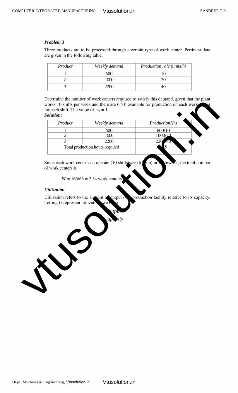
Problem 3
Three products are to be processed through a certain type of work center. Pertinent data
are given in the following table.
Product Weekly demand Production rale (units/hi
1 600 10
2 1000 20
3 2200 40
Determine the number of work centers required to satisfy this demand, given that the plant
works 10 shifts per week and there are 6.5 h available for production on each work center
for each shift. The value of nm = 1.
Solution:
Product Weekly demand ProductionHrs
1 600 600/10 2 1000 1000/20
3 2200 2200/40
Total production hours required 165
Since each work center can operate (10 shifts/week)(6.5 h) or 65 h/week, the total number
of work centers is
W = 165/65 = 2.54 work centers �3
Utilization
Utilization refers to the amount of output of a production facility relative to its capacity.
Letting U represent utilization, we have
�
�
�
�
�
�
�
�
�
�
�
�
�
�
�
�
�
OutputU
Capacity=
COMPUTER INTEGRATED MANUFACTURING SANDEEP T R
Dept. Mechanical Engineering, Vtusolution.in
Vtusolution.in
Vtusolution.in
vtuso
lution
.in

�
�
Problem 4
A production machine is operated 65 h/week at full capacity. Its production rate is 20
units/hr. During a certain week, the machine produced 1000 good parts and was idle the
remaining time.
(a) Determine the production capacity of the machine.
(b) What was the utilization of the machine during the week under consideration?
Solution:
(a) The capacity of the machine can be determined using the assumed 65-h week as
follows:
PC = 65(20) = 1300 units/week
(b) The utilization can be determined as the ratio of the number of parts made during
productive use of the machine relative to its capacity.�
�
�
�
�
�
Availability
The availability is sometimes used as a measure of-reliability for equipment. It is
especially germane for automated production equipment. Availability is defined using two
other reliability terms, the mean lime between failures (MTBF) and the mean time to
repair (MTTR). The MTBF indicates the average length of time between breakdowns of
the piece of equipment. The MTTR indicates the average time required to service the
equipment and place it back into operation when a breakdown does occur:
�
�
�
�
�
�
�
Work-in-process
Work-in-process (WIP) is the amount of product currently located in the factory that is
either being processed or is between processing operations. WIP is inventory that is in
the state of being transformed from raw material to finished product. A rough measure of
work-in-process can be obtained from the equation
�
�
�
�
Where WIP represents the number of units in-process.
100076.92%
1300
OutputU
Capacity= = =
MTBF MTTRAvailability
MTBF
−=
( )W
PC UWIP MLT
S H=
COMPUTER INTEGRATED MANUFACTURING SANDEEP T R
Dept. Mechanical Engineering, Vtusolution.in
Vtusolution.in
Vtusolution.in
vtuso
lution
.in
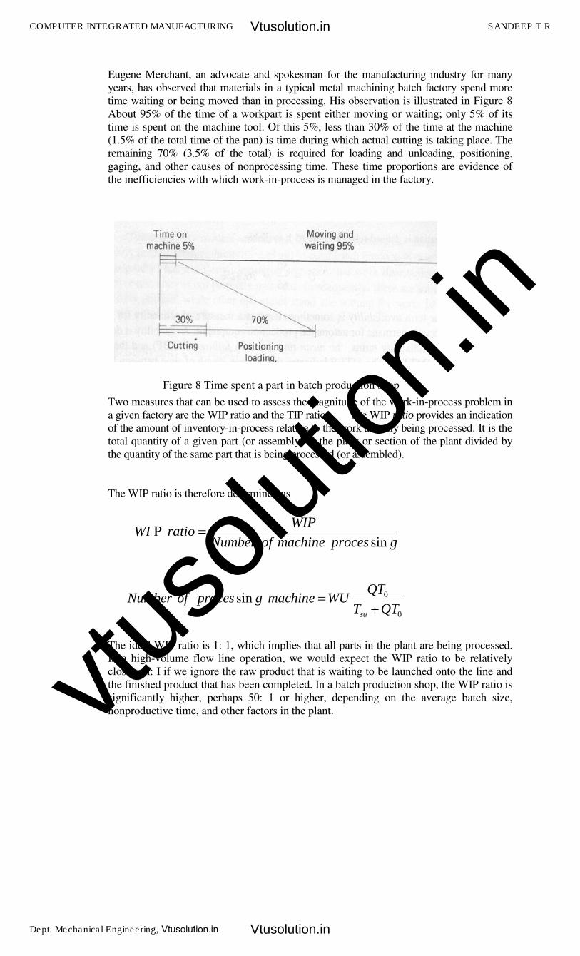
Eugene Merchant, an advocate and spokesman for the manufacturing industry for many
years, has observed that materials in a typical metal machining batch factory spend more
time waiting or being moved than in processing. His observation is illustrated in Figure 8
About 95% of the time of a workpart is spent either moving or waiting; only 5% of its
time is spent on the machine tool. Of this 5%, less than 30% of the time at the machine
(1.5% of the total time of the pan) is time during which actual cutting is taking place. The
remaining 70% (3.5% of the total) is required for loading and unloading, positioning,
gaging, and other causes of nonprocessing time. These time proportions are evidence of
the inefficiencies with which work-in-process is managed in the factory.
�
�
�
�
�
�
�
�
�
�
�
�
�
�
�
Two measures that can be used to assess the magnitude of the work-in-process problem in
a given factory are the WIP ratio and the TIP ratio. The WIP ratio provides an indication
of the amount of inventory-in-process relative to the work actually being processed. It is the
total quantity of a given part (or assembly) in the plant or section of the plant divided by
the quantity of the same part that is being processed (or assembled).
The WIP ratio is therefore determined as
�
�
�
�
�
�
�
�
�
The ideal WIP ratio is 1: 1, which implies that all parts in the plant are being processed.
In a high-volume flow line operation, we would expect the WIP ratio to be relatively
close to I: I if we ignore the raw product that is waiting to be launched onto the line and
the finished product that has been completed. In a batch production shop, the WIP ratio is
significantly higher, perhaps 50: 1 or higher, depending on the average batch size,
nonproductive time, and other factors in the plant.
Figure 8 Time spent a part in batch production shop
Psin
WIPWI ratio
Number of machine proces g=
0
0
sinsu
QTNumber of proces g machine WU
T QT=
+
COMPUTER INTEGRATED MANUFACTURING SANDEEP T R
Dept. Mechanical Engineering, Vtusolution.in
Vtusolution.in
Vtusolution.in
vtuso
lution
.in
The TIP ratio measures the time that the product spends in the plant relative to its actual
processing time. It is computed as the total manufacturing lead time for a pan divided by
the sum of the individual operation times for the part.
�
�
�
Again, the ideal TIP ratio is 1: 1, and again it is very difficult to achieve such a low
ratio in practice. In the Merchant observation of Figure 2.6, the TIP ratio = 20: 1.
It should be noted that the WIP and TIP ratios reduce to the same value in our simplified
model of manufacturing presented in this section. This can be demonstrated
mathematically. In an actual factory situation, the WIP and TIP ratios would not nec-
essarily be equal, owing to the complexities and realities encountered in the real world. For
example, assembled products create complications in evaluating the ratio values because
of the combination of parts into one assembly.
�
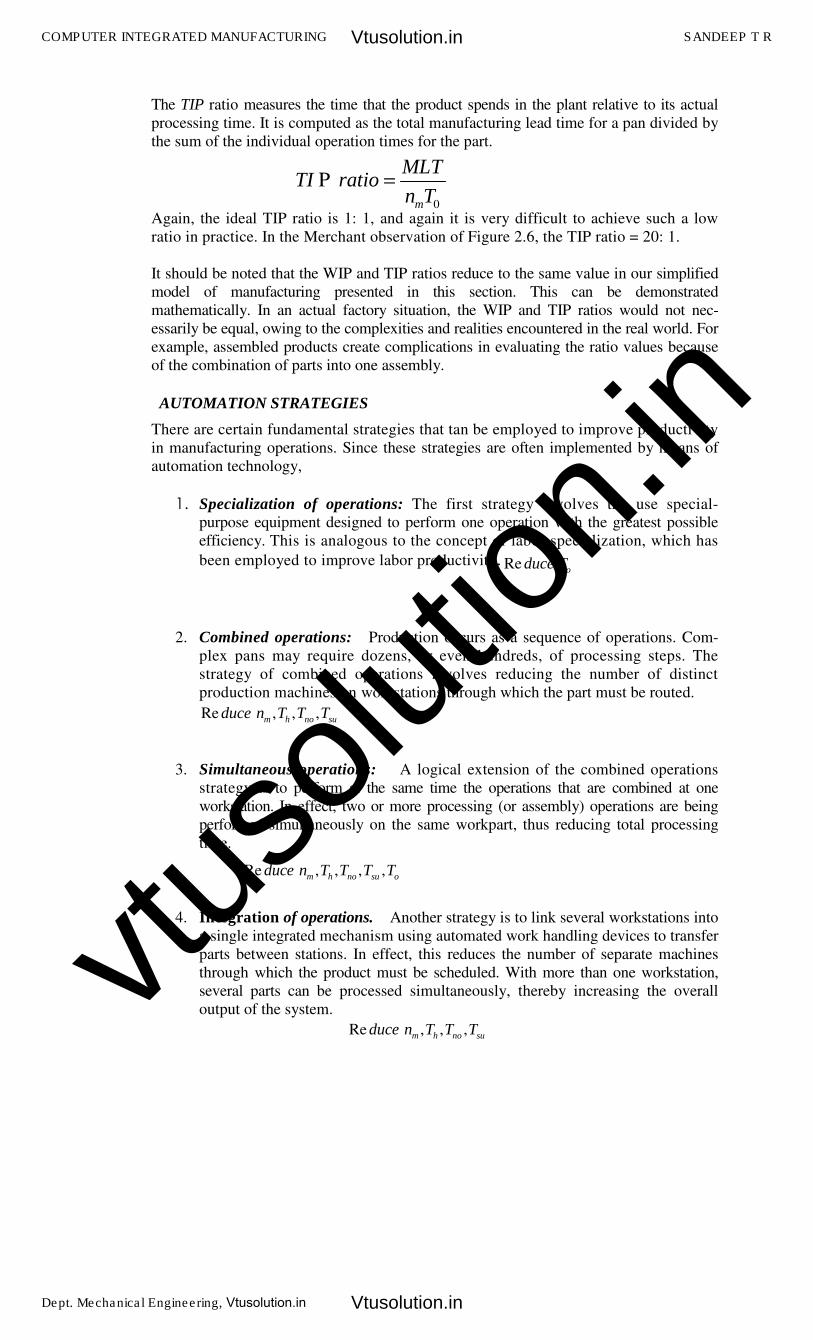
AUTOMATION STRATEGIES
There are certain fundamental strategies that tan be employed to improve productivity
in manufacturing operations. Since these strategies are often implemented by means of
automation technology,
�� Specialization of operations: The first strategy involves the use special-
purpose equipment designed to perform one operation with the greatest possible
efficiency. This is analogous to the concept of labor specialization, which has
been employed to improve labor productivity���
�
�
�
2. Combined operations: Production occurs as a sequence of operations. Com-
plex pans may require dozens, or even hundreds, of processing steps. The
strategy of combined operations involves reducing the number of distinct
production machines on workstations through which the part must be routed.
�
�
�
3. Simultaneous operations: A logical extension of the combined operations
strategy is to perform at the same time the operations that are combined at one
workstation. In effect, two or more processing (or assembly) operations are being
performed simultaneously on the same workpart, thus reducing total processing
time.
�
4. Integration of operations. Another strategy is to link several workstations into
a single integrated mechanism using automated work handling devices to transfer
parts between stations. In effect, this reduces the number of separate machines
through which the product must be scheduled. With more than one workstation,
several parts can be processed simultaneously, thereby increasing the overall
output of the system.
�
0
Pm
MLTTI ratio
n T=
Reo
duce T
Re , , ,m h no su
duce n T T T
Re , , , ,m h no su o
duce n T T T T
Re , , ,m h no su
duce n T T T
COMPUTER INTEGRATED MANUFACTURING SANDEEP T R
Dept. Mechanical Engineering, Vtusolution.in
Vtusolution.in
Vtusolution.in
vtuso
lution
.in
�
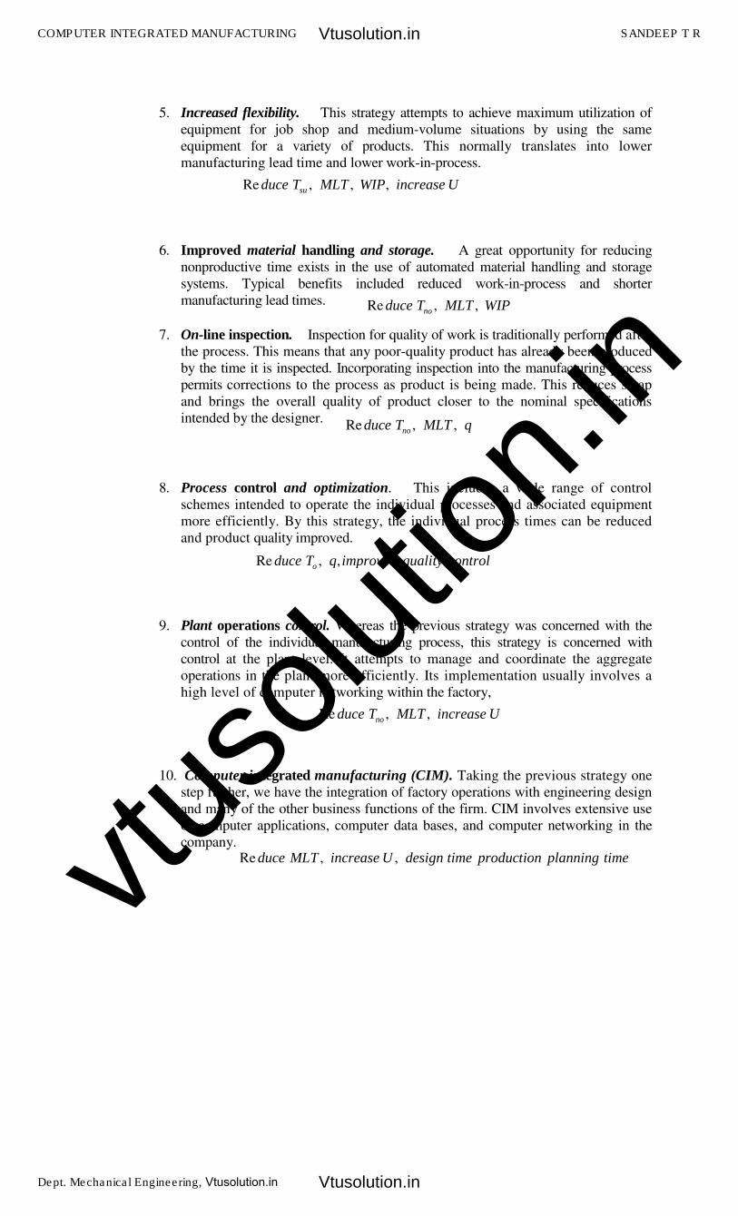
5. Increased flexibility. This strategy attempts to achieve maximum utilization of
equipment for job shop and medium-volume situations by using the same
equipment for a variety of products. This normally translates into lower
manufacturing lead time and lower work-in-process.
�
�
�
�
6. Improved material handling and storage. A great opportunity for reducing
nonproductive time exists in the use of automated material handling and storage
systems. Typical benefits included reduced work-in-process and shorter
manufacturing lead times.
�
7. On-line inspection. Inspection for quality of work is traditionally performed after
the process. This means that any poor-quality product has already been produced
by the time it is inspected. Incorporating inspection into the manufacturing process
permits corrections to the process as product is being made. This reduces scrap
and brings the overall quality of product closer to the nominal specifications
intended by the designer.
�
�
�
8. Process control and optimization. This includes a wide range of control
schemes intended to operate the individual processes and associated equipment
more efficiently. By this strategy, the individual process times can be reduced
and product quality improved.
�
�
�
�
9. Plant operations control. Whereas the previous strategy was concerned with the
control of the individual manufacturing process, this strategy is concerned with
control at the plant level. It attempts to manage and coordinate the aggregate
operations in the plant more efficiently. Its implementation usually involves a
high level of computer networking within the factory,
10. Computer integrated manufacturing (CIM). Taking the previous strategy one
step further, we have the integration of factory operations with engineering design
and many of the other business functions of the firm. CIM involves extensive use
of computer applications, computer data bases, and computer networking in the
company.
Re , , ,suduce T MLT WIP increase U
Re , ,noduce T MLT WIP
Re , ,noduce T MLT q
Re , ,oduce T q improved quality control
Re , ,noduce T MLT increase U
Re , ,duce MLT increase U design time production planning time
COMPUTER INTEGRATED MANUFACTURING SANDEEP T R
Dept. Mechanical Engineering, Vtusolution.in
Vtusolution.in
Vtusolution.in
vtuso
lution
.in
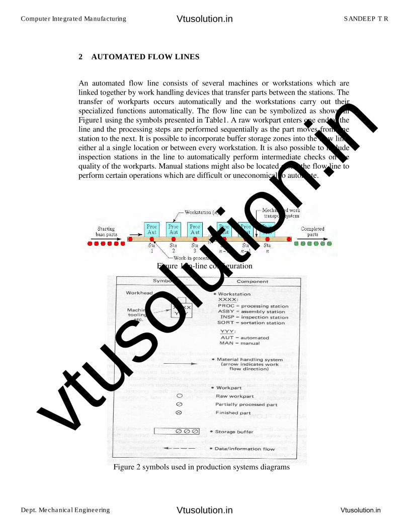
2 AUTOMATED FLOW LINES
An automated flow line consists of several machines or workstations which are
linked together by work handling devices that transfer parts between the stations. The
transfer of workparts occurs automatically and the workstations carry out their
specialized functions automatically. The flow line can be symbolized as shown in
Figure1 using the symbols presented in Table1. A raw workpart enters one end of the
line and the processing steps are performed sequentially as the part moves from one
station to the next. It is possible to incorporate buffer storage zones into the flow line,
either al a single location or between every workstation. It is also possible to include
inspection stations in the line to automatically perform intermediate checks on the
quality of the workparts. Manual stations might also be located along the flow line to
perform certain operations which are difficult or uneconomical to automate.
Figure 2 symbols used in production systems diagrams
Figure 1 In-line configuration
Computer Integrated Manufacturing SANDEEP T R
Dept. Mechanical Engineering Vtusolution.in
Vtusolution.in
Vtusolution.in
vtuso
lution
.in
The objectives of the use of flow line automation are, therefore:
• To reduce labor costs
• To increase production rates
• To reduce work-in-process
• To minimize distances moved between operations
• To achieve specialization of operations
• To achieve integration of operations
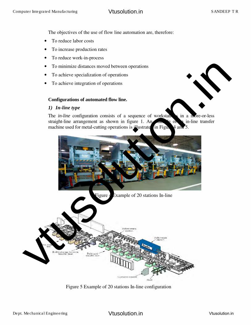
Configurations of automated flow line.
1) In-line type
The in-line configuration consists of a sequence of workstations in a more-or-less
straight-line arrangement as shown in figure 1. An example of an in-line transfer
machine used for metal-cutting operations is illustrated in Figure 4 and 5.
Figure 5 Example of 20 stations In-line configuration
Figure 4 Example of 20 stations In-line
Computer Integrated Manufacturing SANDEEP T R
Dept. Mechanical Engineering Vtusolution.in
Vtusolution.in
Vtusolution.in
vtuso
lution
.in

2) Segmented In-Line Type
The segmented in-line configuration consists of two or more straight-line arrangement
which are usually perpendicular to each other with L-Shaped or U-shaped or
Rectangular shaped as shown in figure 5-7. The flow of work can take a few 90°
turns, either for workpieces reorientation, factory layout limitations, or other reasons,
and still qualify as a straight-line configuration.
Figure 5 L-shaped configuration
Figure 6 U-shaped configuration
Figure 7 Rectangular-shaped configuration
Computer Integrated Manufacturing SANDEEP T R
Dept. Mechanical Engineering Vtusolution.in
Vtusolution.in
Vtusolution.in
vtuso
lution
.in
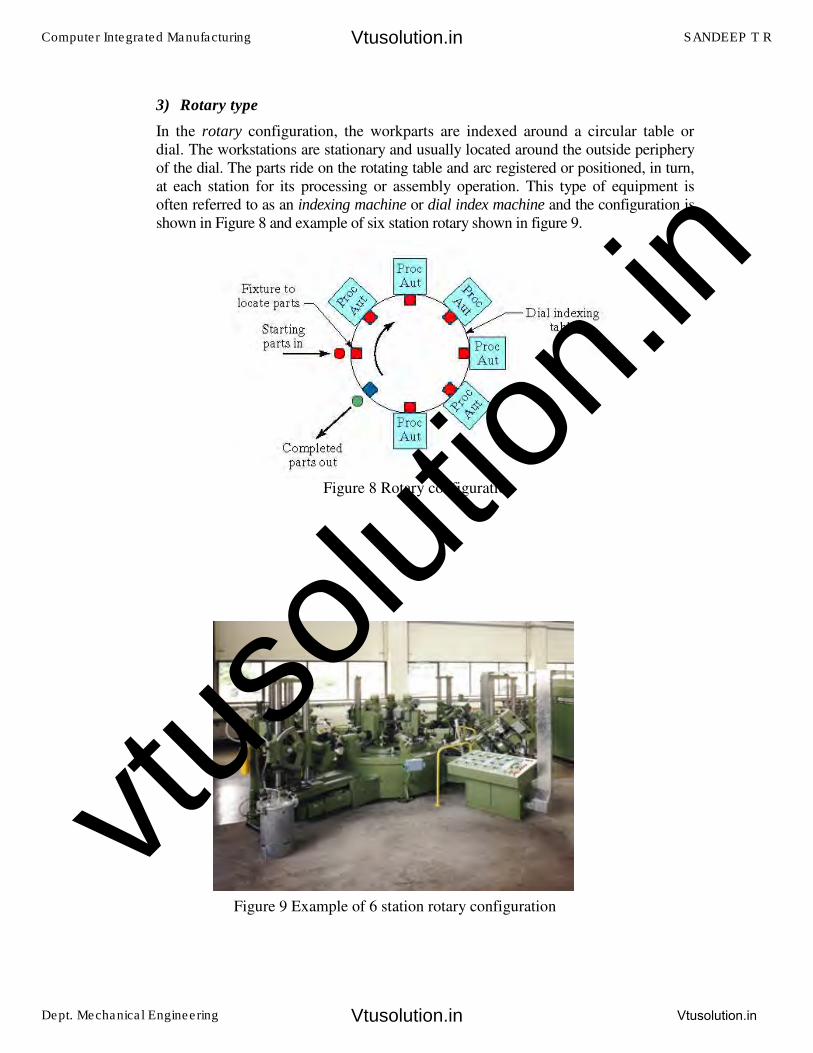
3) Rotary type
In the rotary configuration, the workparts are indexed around a circular table or
dial. The workstations are stationary and usually located around the outside periphery
of the dial. The parts ride on the rotating table and arc registered or positioned, in turn,
at each station for its processing or assembly operation. This type of equipment is
often referred to as an indexing machine or dial index machine and the configuration is
shown in Figure 8 and example of six station rotary shown in figure 9.
Figure 8 Rotary configuration
Figure 9 Example of 6 station rotary configuration
Computer Integrated Manufacturing SANDEEP T R
Dept. Mechanical Engineering Vtusolution.in
Vtusolution.in
Vtusolution.in
vtuso
lution
.in
METHODS OF WORKPART TRANSPORT
The transfer mechanism of the automated flow line must not only move the partially
completed workparts or assemblies between adjacent stations, it must also orient and
locate the parts in the correct position for processing at each station. The general
methods of transporting workpieces on flow lines can be classified into the following
three categories:
1. Continuous transfer
2. Intermittent or synchronous transfer
3. Asynchronous or power-and-free transfer
The most appropriate type of transport system for a given application depends on
such factors as:
� The types of operation to be performed
� The number of stations on the line
� The weight and size of the work parts
� Whether manual stations are included on the line
� Production rate requirements
� Balancing the various process times on the line
1) Continuous transfer
With the continuous method of transfer, the workparts are moved continuously at
Constant speed. This requires the workheads to move during processing in order to
maintain continuous registration with the workpart. For some types of operations,
this movement of the workheads during processing is not feasible. It would be
difficult, for example, to use this type of system on a machining transfer line
because of inertia problems due to the size and weight of the workheads. In other
cases, continuous transfer would be very practical. Examples of its use are in
beverage bottling operations, packaging, manual assembly operations where the
human operator can move with the moving flow line, and relatively simple
automatic assembly tasks. In some bottling operations, for instance, the bottles are
transported around a continuously rotating drum. Beverage is discharged into the
moving bottles by spouts located at the drum's periphery. The advantage of this
application is that the liquid beverage is kept moving at a steady speed and hence
there are no inertia problems.
Continuous transfer systems are relatively easy to design and fabricate and can
achieve a high rate of production.
Computer Integrated Manufacturing SANDEEP T R
Dept. Mechanical Engineering Vtusolution.in
Vtusolution.in
Vtusolution.in
vtuso
lution
.in
2) Intermittent transfer
As the name suggests, in this method the workpieces are transported with an
intermittent or discontinuous motion. The workstations are fixed in position and the
parts are moved between stations and then registered at the proper locations for
processing. All workparts are transported at the same time and, for this reason, the
term "synchronous transfer system" is also used to describe this method of
workpart transport.
3) Asynchronous transfer
This system of transfer, also referred to as a "power-and-free system," allows each
workpart to move to the next station when processing at the current station has been
completed. Each part moves independently of other parts. Hence, some parts are being
processed on the line at the same time that others are being transported between sta-
tions.
Asynchronous transfer systems offer the opportunity for greater flexibility than do the
other two systems, and this flexibility can be a great advantage in certain circumstances.
In-process storage of workparts can be incorporated into the asynchronous systems
with relative ease. Power-and-free systems can also compensate for line balancing
problems where there are significant differences in process times between stations.
Parallel stations or several series stations can be used for the longer operations, and
single stations can be used for the shorter operations. Therefore, the average
production rates can be approximately equalized. Asynchronous lines are often used
where there are one or more manually operated stations and cycle-time variations
would be a problem on either the continuous or synchronous transport systems. Larger
workparts can be handled on the asynchronous systems. A disadvantage of the power-
and-free systems is that the cycle rates are generally slower than for the other types.
Computer Integrated Manufacturing SANDEEP T R
Dept. Mechanical Engineering Vtusolution.in
Vtusolution.in
Vtusolution.in
vtuso
lution
.in
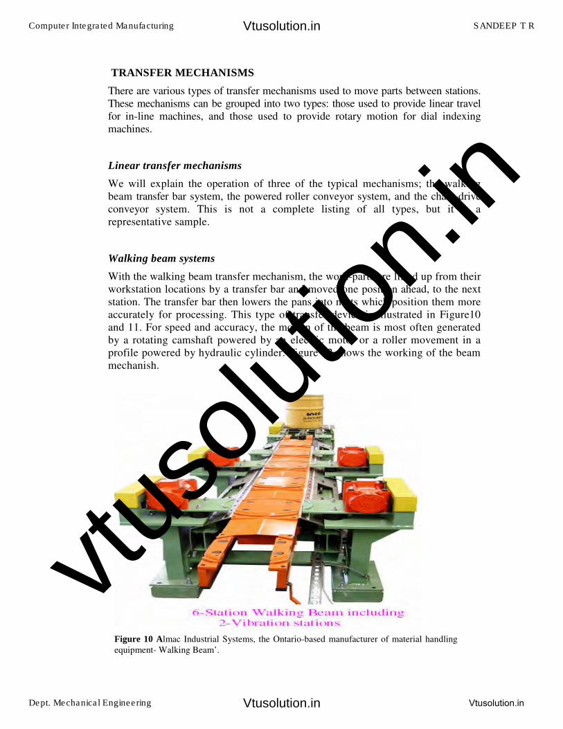
TRANSFER MECHANISMS
There are various types of transfer mechanisms used to move parts between stations.
These mechanisms can be grouped into two types: those used to provide linear travel
for in-line machines, and those used to provide rotary motion for dial indexing
machines.
Linear transfer mechanisms
We will explain the operation of three of the typical mechanisms; the walking
beam transfer bar system, the powered roller conveyor system, and the chain-drive
conveyor system. This is not a complete listing of all types, but it is a
representative sample.
Walking beam systems
With the walking beam transfer mechanism, the work-parts are lifted up from their
workstation locations by a transfer bar and moved one position ahead, to the next
station. The transfer bar then lowers the pans into nests which position them more
accurately for processing. This type of transfer device is illustrated in Figure10
and 11. For speed and accuracy, the motion of the beam is most often generated
by a rotating camshaft powered by an electric motor or a roller movement in a
profile powered by hydraulic cylinder. Figure 12 shows the working of the beam
mechanish.
Figure 10 Almac Industrial Systems, the Ontario-based manufacturer of material handling
equipment- Walking Beam’.
Computer Integrated Manufacturing SANDEEP T R
Dept. Mechanical Engineering Vtusolution.in
Vtusolution.in
Vtusolution.in
vtuso
lution
.in
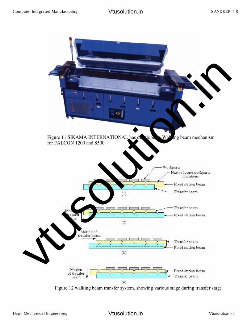
Figure 11 SIKAMA INTERNATIONAL has developed a Walking beam mechanism
for FALCON 1200 and 8500
Figure 12 walking beam transfer system, showing various stage during transfer stage
Computer Integrated Manufacturing SANDEEP T R
Dept. Mechanical Engineering Vtusolution.in
Vtusolution.in
Vtusolution.in
vtuso
lution
.in
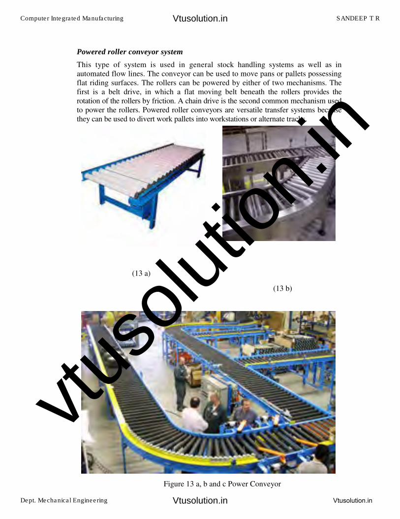
Powered roller conveyor system
This type of system is used in general stock handling systems as well as in
automated flow lines. The conveyor can be used to move pans or pallets possessing
flat riding surfaces. The rollers can be powered by either of two mechanisms. The
first is a belt drive, in which a flat moving belt beneath the rollers provides the
rotation of the rollers by friction. A chain drive is the second common mechanism used
to power the rollers. Powered roller conveyors are versatile transfer systems because
they can be used to divert work pallets into workstations or alternate tracks.
(13 a)
(13 b)
Figure 13 a, b and c Power Conveyor
Computer Integrated Manufacturing SANDEEP T R
Dept. Mechanical Engineering Vtusolution.in
Vtusolution.in
Vtusolution.in
vtuso
lution
.in
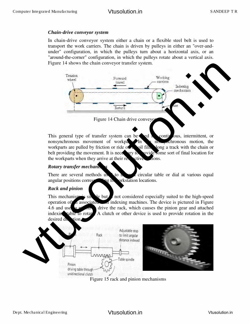
Chain-drive conveyor system
In chain-drive conveyor system either a chain or a flexible steel belt is used to
transport the work carriers. The chain is driven by pulleys in either an "over-and-
under" configuration, in which the pulleys turn about a horizontal axis, or an
"around-the-corner" configuration, in which the pulleys rotate about a vertical axis.
Figure 14 shows the chain conveyor transfer system.
This general type of transfer system can be used for continuous, intermittent, or
nonsynchronous movement of workparts. In the nonsynchronous motion, the
workparts are pulled by friction or ride on an oil film along a track with the chain or
belt providing the movement. It is necessary to provide some sort of final location for
the workparts when they arrive at their respective stations.
Rotary transfer mechanisms
There are several methods used to index a circular table or dial at various equal
angular positions corresponding to workstation locations.
Rack and pinion
This mechanism is simple but is not considered especially suited to the high-speed
operation often associated with indexing machines. The device is pictured in Figure
4.6 and uses a piston to drive the rack, which causes the pinion gear and attached
indexing table to rotate, A clutch or other device is used to provide rotation in the
desired direction.
Figure 14 Chain drive conveyor
Figure 15 rack and pinion mechanisms
Computer Integrated Manufacturing SANDEEP T R
Dept. Mechanical Engineering Vtusolution.in
Vtusolution.in
Vtusolution.in
vtuso
lution
.in
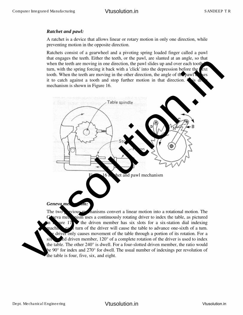
Ratchet and pawl:
A ratchet is a device that allows linear or rotary motion in only one direction, while
preventing motion in the opposite direction.
Ratchets consist of a gearwheel and a pivoting spring loaded finger called a pawl
that engages the teeth. Either the teeth, or the pawl, are slanted at an angle, so that
when the teeth are moving in one direction, the pawl slides up and over each tooth in
turn, with the spring forcing it back with a 'click' into the depression before the next
tooth. When the teeth are moving in the other direction, the angle of the pawl causes
it to catch against a tooth and stop further motion in that direction. This drive
mechanism is shown in Figure 16.
Geneva mechanism:
The two previous mechanisms convert a linear motion into a rotational motion. The
Geneva mechanism uses a continuously rotating driver to index the table, as pictured
in Figure 17. If the driven member has six slots for a six-station dial indexing
machine, each turn of the driver will cause the table to advance one-sixth of a turn.
The driver only causes movement of the table through a portion of its rotation. For a
six-slotted driven member, 120° of a complete rotation of the driver is used to index
the table. The other 240° is dwell. For a four-slotted driven member, the ratio would
be 90° for index and 270° for dwell. The usual number of indexings per revolution of
the table is four, five, six, and eight.
Figure 16 Rachet and pawl mechanism
Computer Integrated Manufacturing SANDEEP T R
Dept. Mechanical Engineering Vtusolution.in
Vtusolution.in
Vtusolution.in
vtuso
lution
.in
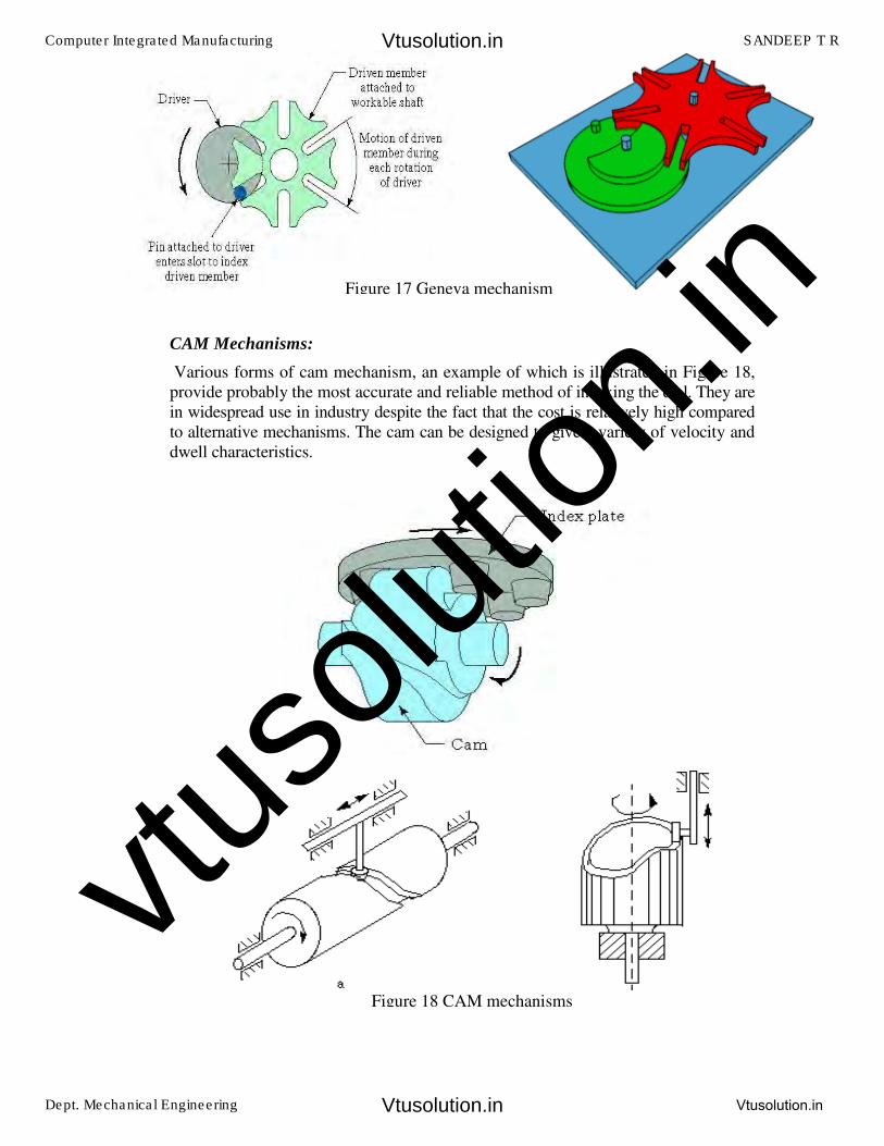
CAM Mechanisms:
Various forms of cam mechanism, an example of which is illustrated in Figure 18,
provide probably the most accurate and reliable method of indexing the dial. They are
in widespread use in industry despite the fact that the cost is relatively high compared
to alternative mechanisms. The cam can be designed to give a variety of velocity and
dwell characteristics.
Figure 17 Geneva mechanism
Figure 18 CAM mechanisms
Computer Integrated Manufacturing SANDEEP T R
Dept. Mechanical Engineering Vtusolution.in
Vtusolution.in
Vtusolution.in
vtuso
lution
.in
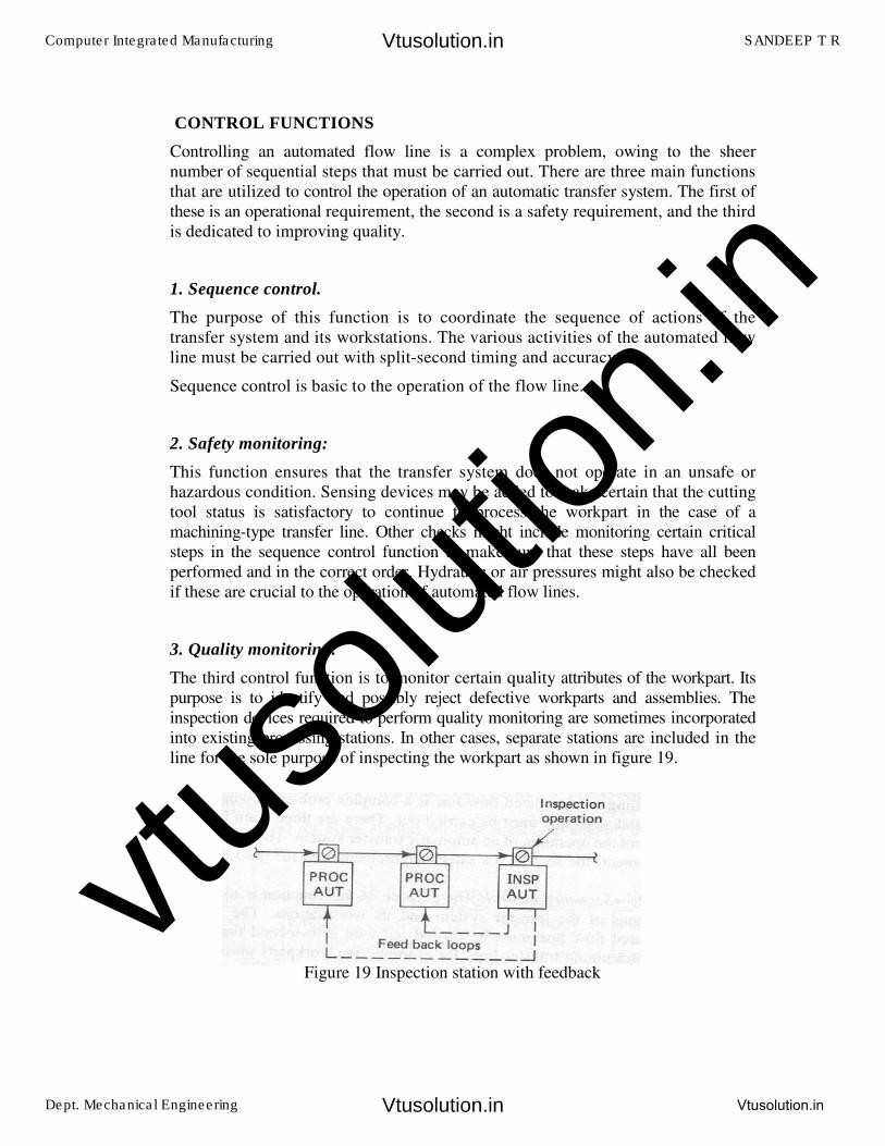
CONTROL FUNCTIONS
Controlling an automated flow line is a complex problem, owing to the sheer
number of sequential steps that must be carried out. There are three main functions
that are utilized to control the operation of an automatic transfer system. The first of
these is an operational requirement, the second is a safety requirement, and the third
is dedicated to improving quality.
1. Sequence control.
The purpose of this function is to coordinate the sequence of actions of the
transfer system and its workstations. The various activities of the automated flow
line must be carried out with split-second timing and accuracy.
Sequence control is basic to the operation of the flow line.
2. Safety monitoring:
This function ensures that the transfer system does not operate in an unsafe or
hazardous condition. Sensing devices may be added to make certain that the cutting
tool status is satisfactory to continue to process the workpart in the case of a
machining-type transfer line. Other checks might include monitoring certain critical
steps in the sequence control function to make sure that these steps have all been
performed and in the correct order. Hydraulic or air pressures might also be checked
if these are crucial to the operation of automated flow lines.
3. Quality monitoring:
The third control function is to monitor certain quality attributes of the workpart. Its
purpose is to identify and possibly reject defective workparts and assemblies. The
inspection devices required to perform quality monitoring are sometimes incorporated
into existing processing stations. In other cases, separate stations are included in the
line for the sole purpose of inspecting the workpart as shown in figure 19.
Figure 19 Inspection station with feedback
Computer Integrated Manufacturing SANDEEP T R
Dept. Mechanical Engineering Vtusolution.in
Vtusolution.in
Vtusolution.in
vtuso
lution
.in
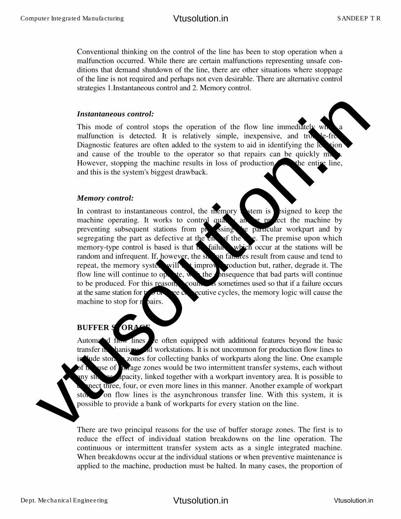
Conventional thinking on the control of the line has been to stop operation when a
malfunction occurred. While there are certain malfunctions representing unsafe con-
ditions that demand shutdown of the line, there are other situations where stoppage
of the line is not required and perhaps not even desirable. There are alternative control
strategies 1.Instantaneous control and 2. Memory control.
Instantaneous control:
This mode of control stops the operation of the flow line immediately when a
malfunction is detected. It is relatively simple, inexpensive, and trouble-free.
Diagnostic features are often added to the system to aid in identifying the location
and cause of the trouble to the operator so that repairs can be quickly made.
However, stopping the machine results in loss of production from the entire line,
and this is the system's biggest drawback.
Memory control:
In contrast to instantaneous control, the memory system is designed to keep the
machine operating. It works to control quality and/or protect the machine by
preventing subsequent stations from processing the particular workpart and by
segregating the part as defective at the end of the line. The premise upon which
memory-type control is based is that the failures which occur at the stations will be
random and infrequent. If, however, the station failures result from cause and tend to
repeat, the memory system will not improve production but, rather, degrade it. The
flow line will continue to operate, with the consequence that bad parts will continue
to be produced. For this reason, a counter is sometimes used so that if a failure occurs
at the same station for two or three consecutive cycles, the memory logic will cause the
machine to stop for repairs.
BUFFER STORAGE
Automated flow lines are often equipped with additional features beyond the basic
transfer mechanisms and workstations. It is not uncommon for production flow lines to
include storage zones for collecting banks of workparts along the line. One example
of the use of storage zones would be two intermittent transfer systems, each without
any storage capacity, linked together with a workpart inventory area. It is possible to
connect three, four, or even more lines in this manner. Another example of workpart
storage on flow lines is the asynchronous transfer line. With this system, it is
possible to provide a bank of workparts for every station on the line.
There are two principal reasons for the use of buffer storage zones. The first is to
reduce the effect of individual station breakdowns on the line operation. The
continuous or intermittent transfer system acts as a single integrated machine.
When breakdowns occur at the individual stations or when preventive maintenance is
applied to the machine, production must be halted. In many cases, the proportion of
Computer Integrated Manufacturing SANDEEP T R
Dept. Mechanical Engineering Vtusolution.in
Vtusolution.in
Vtusolution.in
vtuso
lution
.in
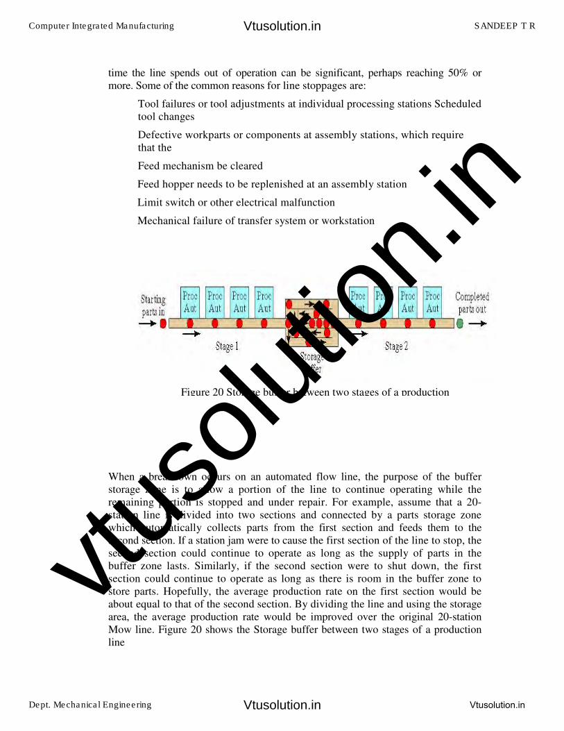
time the line spends out of operation can be significant, perhaps reaching 50% or
more. Some of the common reasons for line stoppages are:
Tool failures or tool adjustments at individual processing stations Scheduled
tool changes
Defective workparts or components at assembly stations, which require
that the
Feed mechanism be cleared
Feed hopper needs to be replenished at an assembly station
Limit switch or other electrical malfunction
Mechanical failure of transfer system or workstation
When a breakdown occurs on an automated flow line, the purpose of the buffer
storage zone is to allow a portion of the line to continue operating while the
remaining portion is stopped and under repair. For example, assume that a 20-
station line is divided into two sections and connected by a parts storage zone
which automatically collects parts from the first section and feeds them to the
second section. If a station jam were to cause the first section of the line to stop, the
second section could continue to operate as long as the supply of parts in the
buffer zone lasts. Similarly, if the second section were to shut down, the first
section could continue to operate as long as there is room in the buffer zone to
store parts. Hopefully, the average production rate on the first section would be
about equal to that of the second section. By dividing the line and using the storage
area, the average production rate would be improved over the original 20-station
Mow line. Figure 20 shows the Storage buffer between two stages of a production
line
Figure 20 Storage buffer between two stages of a production
Computer Integrated Manufacturing SANDEEP T R
Dept. Mechanical Engineering Vtusolution.in
Vtusolution.in
Vtusolution.in
vtuso
lution
.in
Reasons for using storage buffers:
– To reduce effect of station breakdowns
– To provide a bank of parts to supply the line
– To provide a place to put the output of the line
– To allow curing time or other required delay
– To smooth cycle time variations
– To store parts between stages with different production rates
The disadvantages of buffer storage on flow lines are increased factory floor space,
higher in-process inventory, more material handling equipment, and greater
complexity of the overall flow line system. The benefits of buffer storage are often
great enough to more than compensate for these disadvantages.
AUTOMATION FOR MACHINING OPERATIONS
Transfer systems have been designed to perform a great variety of different metal-
cutting processes. In fact, it is difficult to think of machining operations that must be
excluded from the list. Typical applications include operations such as milling, boring,
drilling, reaming, and tapping. However, it is also feasible to carry out operations such
as turning and grinding on transfer-type systems.
There are various types of mechanized and automated machines that perform a
sequence of operations simultaneously on different work parts. These include dial
indexing machines, trunnion machines, and transfer lines. To consider these machines
in approximately the order of increasing complexity, we begin with one that really does
not belong in the list at all, the single-station machine.
Single-station machine
These mechanized production machines perform several operations on a single workpart
which is fixtured in one position throughout the cycle. The operations are performed
on several different surfaces by work heads located around the piece. The available
space surrounding a stationary workpiece limits the number of machining heads
that can be used. This limit on the number of operations is the principal
disadvantage of the single-station machine. Production rates are usually low to
medium. The single station machine is as shown in figure 21.
Computer Integrated Manufacturing SANDEEP T R
Dept. Mechanical Engineering Vtusolution.in
Vtusolution.in
Vtusolution.in
vtuso
lution
.in
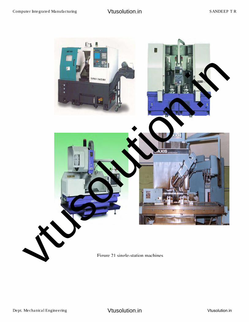
Figure 21 single-station machines
Computer Integrated Manufacturing SANDEEP T R
Dept. Mechanical Engineering Vtusolution.in
Vtusolution.in
Vtusolution.in
vtuso
lution
.in
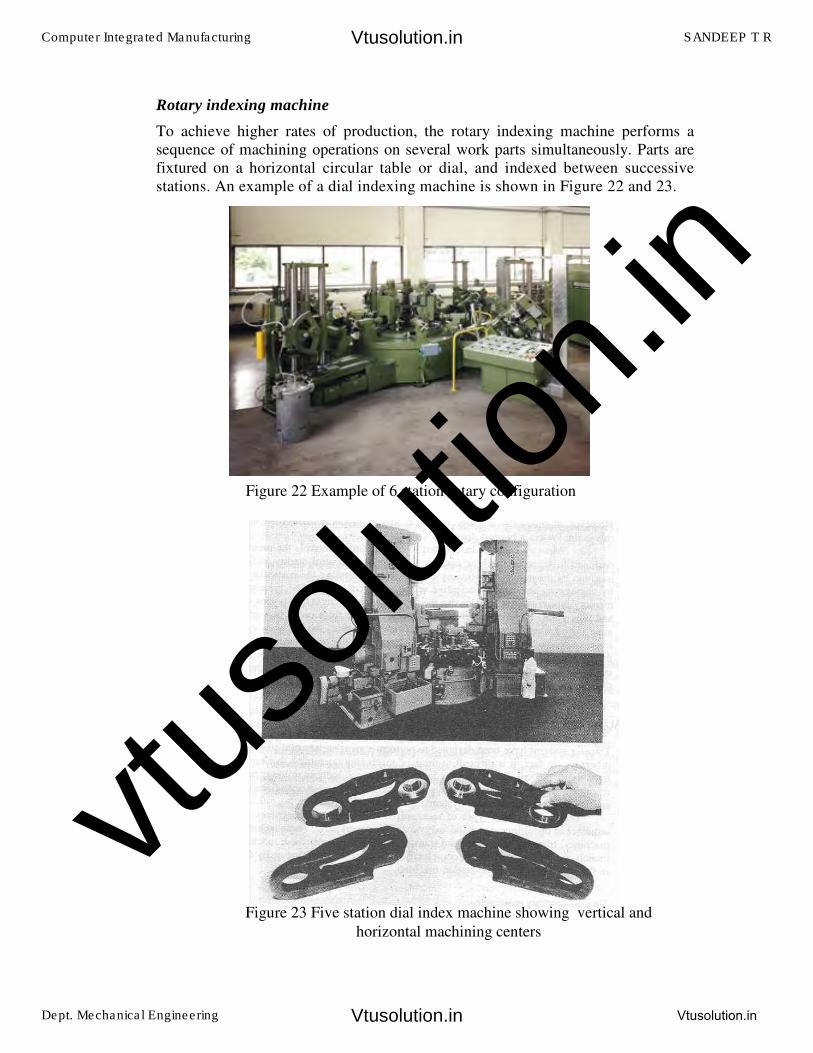
Rotary indexing machine
To achieve higher rates of production, the rotary indexing machine performs a
sequence of machining operations on several work parts simultaneously. Parts are
fixtured on a horizontal circular table or dial, and indexed between successive
stations. An example of a dial indexing machine is shown in Figure 22 and 23.
Figure 22 Example of 6 station rotary configuration
Figure 23 Five station dial index machine showing vertical and
horizontal machining centers
Computer Integrated Manufacturing SANDEEP T R
Dept. Mechanical Engineering Vtusolution.in
Vtusolution.in
Vtusolution.in
vtuso
lution
.in
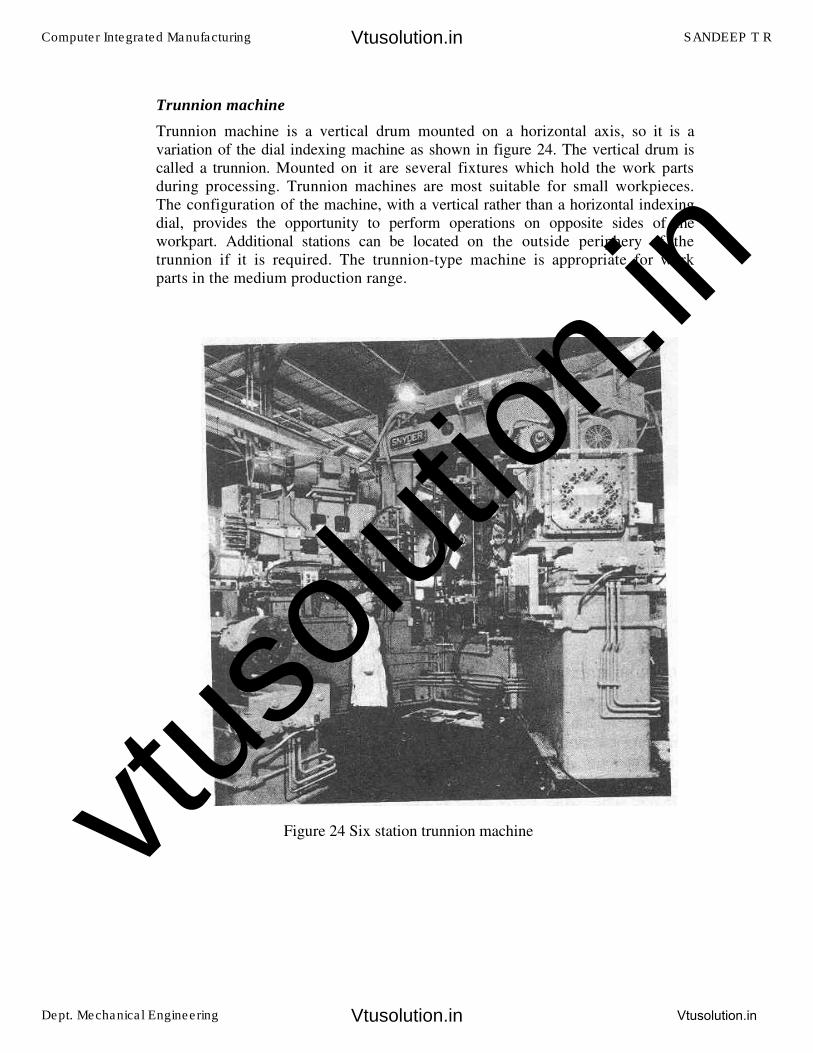
Trunnion machine
Trunnion machine is a vertical drum mounted on a horizontal axis, so it is a
variation of the dial indexing machine as shown in figure 24. The vertical drum is
called a trunnion. Mounted on it are several fixtures which hold the work parts
during processing. Trunnion machines are most suitable for small workpieces.
The configuration of the machine, with a vertical rather than a horizontal indexing
dial, provides the opportunity to perform operations on opposite sides of the
workpart. Additional stations can be located on the outside periphery of the
trunnion if it is required. The trunnion-type machine is appropriate for work
parts in the medium production range.
Figure 24 Six station trunnion machine
Computer Integrated Manufacturing SANDEEP T R
Dept. Mechanical Engineering Vtusolution.in
Vtusolution.in
Vtusolution.in
vtuso
lution
.in
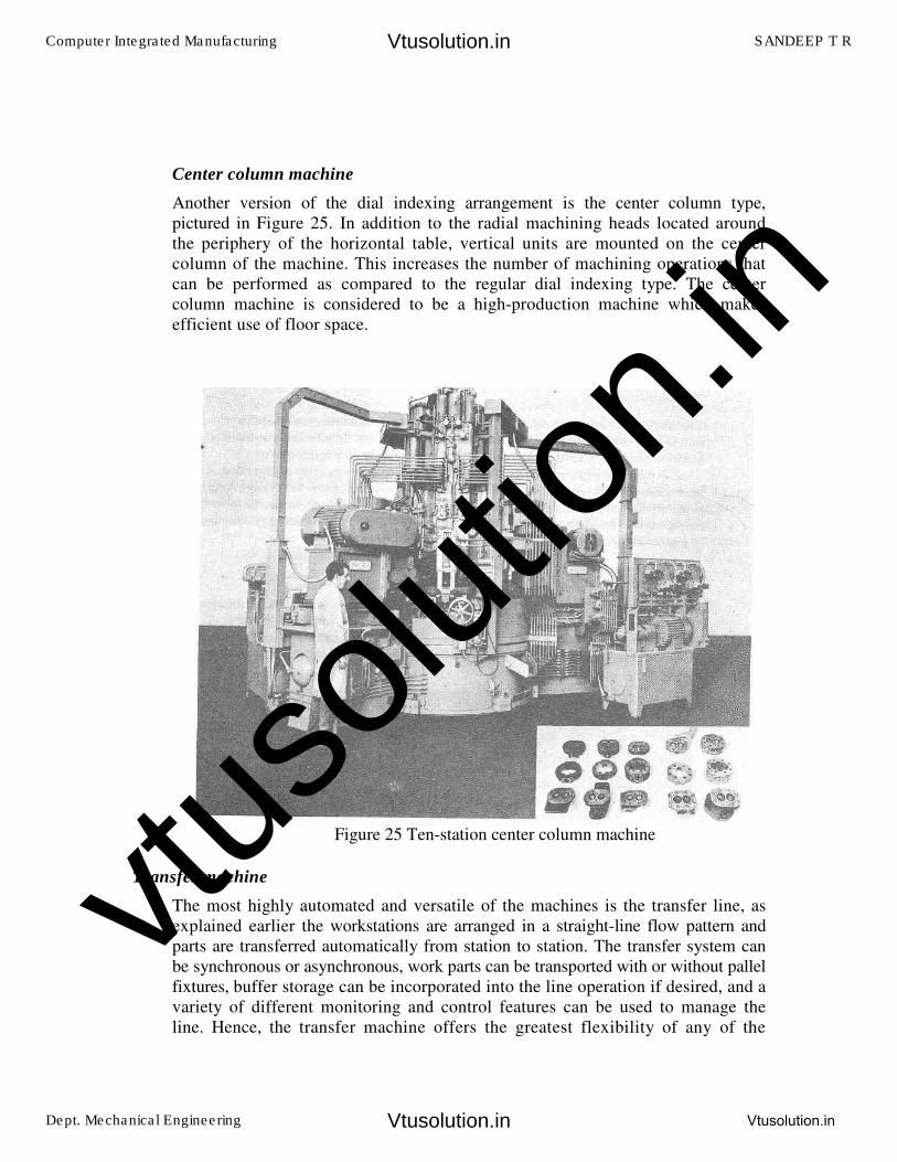
Center column machine
Another version of the dial indexing arrangement is the center column type,
pictured in Figure 25. In addition to the radial machining heads located around
the periphery of the horizontal table, vertical units are mounted on the center
column of the machine. This increases the number of machining operations that
can be performed as compared to the regular dial indexing type. The center
column machine is considered to be a high-production machine which makes
efficient use of floor space.
Transfer machine
The most highly automated and versatile of the machines is the transfer line, as
explained earlier the workstations are arranged in a straight-line flow pattern and
parts are transferred automatically from station to station. The transfer system can
be synchronous or asynchronous, work parts can be transported with or without pallel
fixtures, buffer storage can be incorporated into the line operation if desired, and a
variety of different monitoring and control features can be used to manage the
line. Hence, the transfer machine offers the greatest flexibility of any of the
Figure 25 Ten-station center column machine
Computer Integrated Manufacturing SANDEEP T R
Dept. Mechanical Engineering Vtusolution.in
Vtusolution.in
Vtusolution.in
vtuso
lution
.in
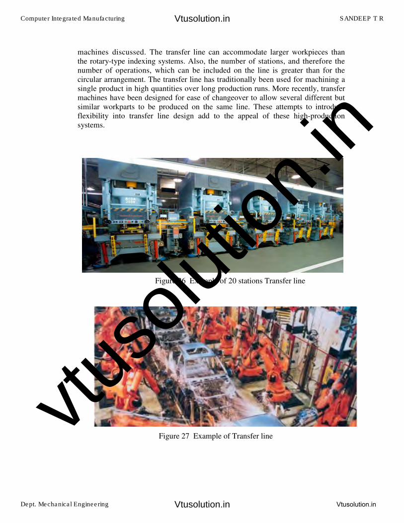
machines discussed. The transfer line can accommodate larger workpieces than
the rotary-type indexing systems. Also, the number of stations, and therefore the
number of operations, which can be included on the line is greater than for the
circular arrangement. The transfer line has traditionally been used for machining a
single product in high quantities over long production runs. More recently, transfer
machines have been designed for ease of changeover to allow several different but
similar workparts to be produced on the same line. These attempts to introduce
flexibility into transfer line design add to the appeal of these high-production
systems.
Figure 26 Example of 20 stations Transfer line
Figure 27 Example of Transfer line
Computer Integrated Manufacturing SANDEEP T R
Dept. Mechanical Engineering Vtusolution.in
Vtusolution.in
Vtusolution.in
vtuso
lution
.in
UNIT 3:
ANALYSIS OF AUTOMATED FLOW LINE & LINE BALANCING
General Terminology & Analysis:
There are two problem areas in analysis of automated flow lines which must be addressed: 1. Process Technology2. Systems Technology
Process Technology refers to the body of knowledge about the theory & principles of the particular manufacturing process used on the production line. E.g. in the manufacturing process, process technology includes the metallurgy & machinability of the work material, the correct applications of the cutting tools, chip control, economics of machining, machine tools alterations & a host of other problems. Many problems encountered in machining can be overcome by application of good machining principles. In each process, a technology is developed by many years of research & practice.
Terminology & Analysis of transfer lines with no Internal storage:
There are a few assumptions that we will have to make about the operation of the Transfer line & rotary indexing machines:
1. The workstations perform operations such as machining & not assembly.2. Processing times at each station are constant though they may not be equal.3. There is synchronous transfer of parts.4. No internal storage of buffers.
In the operation of an automated production line, parts are introduced into the first workstation & are processed and transported at regular intervals to the succeeding stations. This interval defines the ideal cycle time, Tc of the production line. Tc is the processing time for the slowest station of the line plus the transfer time; i.e. :
Tc = max (Tsi) + Tr ---------------- (1)
Tc = ideal cycle on the line (min)
Tsi = processing time at station (min)
Tr = repositioning time, called the transfer time (min)
In equation 1, we use the max (Tsi) because the longest service time establishes the pace ofthe production line. The remaining stations with smaller service times will have to wait for the slowest station. The other stations will be idle.
In the operation of a transfer line, random breakdowns & planned stoppages cause downtime on the line.
Common reasons for downtime on an Automated Production line:
1. Tool failures at workstations.2. Tool adjustments at workstations3. Scheduled tool charges4. Limit switch or other electrical malfunctions.
Computer Integrated Manufacturing SANDEEP T R
Dept. Mechanical Engineering Vtusolution.in
Vtusolution.in
Vtusolution.in
vtuso
lution
.in
5. Mechanical failure of a workstation.6. Mechanical failure of a transfer line.7. Stock outs of starting work parts.8. Insufficient space for completed parts.9. Preventive maintenance on the line worker breaks.
The frequency of the breakdowns & line stoppages can be measured even though they occur randomly when the line stops, it is down for a certain average time for each downtime occurrence. These downtime occurrences cause the actual average production cycle time of the line to be longer than the ideal cycle time.
The actual average production time Tp:
Tp = Tc + FTd ------------------------ 2F = downtime frequency, line stops / cycle Td = downtime per line stop in minutes The downtime Td includes the time for the repair crew to swing back into action, diagnose the cause of failure, fix it & restart the drive.
FTd = downtime averaged on a per cycle basis
Production can be computed as a reciprocal of Tp
Rp = 1 ----------------------------- 3
Tp
Where, Rp = actual average production rate (pc / min)
Tp = the actual average production time
The ideal production rate is given by
Rc = 1 ------------------------------ 4
Tc
Where Rc = ideal production rate (pc / min)
Production rates must be expressed on an hourly basis on automated production lines.
The machine tool builder uses the ideal production rate, Rc, in the proposal for the automated transfer line & calls it as the production rate at 100% efficiency because of downtime. The machine tool builder may ignore the effect of downtime on production rate but it should be stated that the amount of downtime experienced on the line is the responsibility of the company using the production line. Line efficiency refers to the proportion of uptime on the line & is a measure of reliability more than efficiency. Line efficiency can be calculated as follows:
E = Tc = Tc + FTd ----------------- 5
Tp Tc
Computer Integrated Manufacturing SANDEEP T R
Dept. Mechanical Engineering Vtusolution.in
Vtusolution.in
Vtusolution.in
vtuso
lution
.in
Where E = the proportion of uptime on the production line.
An alternative measure of the performance is the proportion of downtime on the line which is given by:
D = FTd = FTd + FTd ----------------- 6 Tp Tc
Where D = proportion of downtime on the line
E + D = 1.0
An important economic measure of the performance of an automated production line is the cost of the unit produced. The cost of 1 piece includes the cost of the starting blank that is to processed, the cost of time on the production line & the cost of the tool consumed. The cost per unit can be expressed as the sum of three factors:
Cpc = Cm + CoTp + Ct ------------------------ 7 Where Cpc = cost per piece (Rs / pc)
Cm = cost per minute to operate the time (Rs / min) Tp = average production time per piece (min / pc) Ct = cost of tooling per piece (Rs / pc) Co = the allocation of capital cost of the equipment over the service life, labour to
operate the line, applicable overheads, maintenance, & other relevant costs all reduced to cost per min.
Problem on Transfer line performance:
A 30 station Transfer line is being proposed to machine a certain component currently produced by conventional methods. The proposal received from the machine tool builder states that the line will operate at a production rate of 100 pc / hr at 100% efficiency. From a similar transfer line it is estimated that breakdowns of all types will occur at a frequency of F = 0.20 breakdowns per cycle & that the average downtime per line stop will be 8.0 minutes. The starting blank that is machined on the line costs Rs. 5.00 per part. The line operates at a cost for 100 parts each & the average cost per tool = Rs. 20 per cutting edge. Compute the following: 1. Production rate2. Line efficiency3. Cost per unit piece produced on the line
Solution:
1. At 100% efficiency, the line produces 100 pc/hr. The reciprocal gives the unit timeor ideal cycle time per piece.
Tc = 1 = 0.010hr / pc = 0.6 mins 100
The average production time per piece is given by:
Computer Integrated Manufacturing SANDEEP T R
Dept. Mechanical Engineering Vtusolution.in
Vtusolution.in
Vtusolution.in
vtuso
lution
.in
Tp = Tc + FTd = 0.60 + 0.20 (8.0) = 0.60 + 1.60 = 2.2 mins / piece
Rp = 1 / 2.2m = 0.45 pc / min = 27 pc / hr
Efficiency is the ratio of the ideal cycle time to actual production time
E = 0.6 / 2.2 = 27 %
Tooling cost per piece
Ct = (30 tools) (Rs 20 / tool) 100 parts
= Rs. 6 / piece
The hourly ratio of Rs 100 / hr to operate the line is equivalent to Rs. 1.66 / min.
Cpc = 5 + 1.66 (2.2) + 6 = 5 + 3.65 + 6 = Rs 14.65 / piece
Upper Bound Approach:
The upper bound approach provides an upper limit on the frequency on the line stops per cycle. In this approach we assume that the part remains on the line for further processing. It is possible that there will be more than one line stop associated with a given part during its sequence of processing operations. Let Pr = probability or frequency of a failure at station i where i = 1, 2,………. �
Station i where i = 1, 2, ……………. �
Since a part is not removed from the line when a station jam occurs it is possible that the part will be associated with a station breakdown at every station. The expected number of lines stops per part passing through the line is obtained by summing the frequencies Pi over the n stations. Since each of the n stations is processing a part of each cycle, then the expected frequency of line stops per cycle is equal to the expected frequency of line stops per part i.e.
� F = � Pi ----------------------------- 8
i = 1 where F = expected frequency of line stops per cycle
Pi = frequency of station break down per cycle, causing a line stop � = number of workstations on the line
If all the Pi are assumed equal, which is unlikely but useful for computation purposes, then
F = �.p where all the Pi are equal ---------------- 9 p = p = ………….. p = p 1 2 �
Computer Integrated Manufacturing SANDEEP T R
Dept. Mechanical Engineering Vtusolution.in
Vtusolution.in
Vtusolution.in
vtuso
lution
.in
Lower Bound Approach:
The lower bound approach gives an estimate of the lower limit on the expected frequency of line stops per cycle. Here we assume that a station breakdown results in destruction of the part, resulting in removal of the part from the line & preventing its subsequent processing at the remaining workstations.
Let Pi = the probability that the workpiece will jam at a particular station i.
Then considering a given part as it proceeds through the line, Pi = probability that the part will jam at station 1
(1 - Pi) = probability that the part will not jam station 1 & thus will available for processing at subsequent stations. A jam at station 2 is contingent on successfully making it through station 1 & therefore the probability that the same part will jam at station 2 is given by
P (1 – P ) 1 2
Generalising the quantity P (1 – Pi - 1) (1 – Pi - 2) = (1 – P2) (1 – P1) Where i = 1,,2, ………. � is the probability that a given part will jam at any station i. Summing all these probabilities from i = 1 through i = � gives the probability or frequency of line stops per cycle.
Probability that the given part will pass through all � stations without a line stop is
� � (1 - Pi) i = 1
Therefore the frequency of line stops per cycle is:
� F = 1 – � (1 - Pi) --------------------------------- 10
i = 1 If all the probabilities, Pi, are equal, Pi = P, then
� F = 1 - (1 - P)
Because of parts removal in the lower bound approach, the number of parts coming of the line is less than the number launched onto the front of the line. If F= frequency of line stops & a part is removed for every line stop, then the proportion of parts produced is (1 - F). This is the yield of the production line. The production rate equation then becomes:
Rap = 1 – F --------------------------------------- 11 Tp
where Rap = average actual production rate of acceptable parts from the line Tp = average cycle rate of the transfer machine Rp = 1 = average cycle rate of the system
Tp
Computer Integrated Manufacturing SANDEEP T R
Dept. Mechanical Engineering Vtusolution.in
Vtusolution.in
Vtusolution.in
vtuso
lution
.in
Example 2 Upper Bound v/s Lower Bound Approach
A 2 station transfer line has an ideal cycle time of Tc = 1.2 mins. The probability of station breakdown per cycle is equal for all stations & P = 0.005 breakdowns / cycle. For each of the upper bound & lower bound determine: a) frequency of line stops per cycleb) average actual production ratec) line efficiency
a) For the Upper bound approach
F = 20 (0.005) = 0.10 lines per cycle 20 20
F = 1 - (1 – 0.005) = 1 – (0.995) = 1 – 0.0946
= 0.0954 line stops per cycle For the Upper bound approach the production rate,
Rp = 1 20
= 0.500 pc / min = 30 pc /hr
For the lower bound approach the production time we calculate by using the formula for F Tp = Tc + F (Td)
= 1.2 + 0.0954 (0.8) = 1.9631 mins
Production rate = 0.9046 1.9631
= 0.4608 pc / min = 27.65 pc / hr
The production rate is about 8% lower than that we computed by the upper bound approach. We should note that:
Rp = 1 0.9631
= 0.5094 cycles / min = 30.56 cycles / hr
which is slightly higher than in the upper bound case.
c) For the upper bound the line efficiency will be
E = 1.2 2.0 = 0.6
= 60 % For the lower bound approach we have
E = 1.2 1.9631
= 0.6113 = 61.13 %
Computer Integrated Manufacturing SANDEEP T R
Dept. Mechanical Engineering Vtusolution.in
Vtusolution.in
Vtusolution.in
vtuso
lution
.in

Line efficiency is greater with lower bound approach even though production rate is lower. This is because lower bound approach leaves fewer parts remaining on the line to jam.
Analysis of Transfer Lines with Storage Buffers:
In an automated production line with no internal storage of parts, the workstations are interdependent. When one station breaks down all other stations on the line are affected either immediately or by the end of a few cycles of operation. The other stations will be forced to stop for one or two reasons 1) starving of stations 2) Blocking of stations Starving on an automated production line means that a workstation is prevented from performing its cycle because it has no part to work on. When a breakdown occurs at any workstation on the line, the stations downstream from the affected station will either immediately or eventually become starved for parts.
Blocking means that a station is prevented from performing its work cycle because it cannot pass the part it just completed to the neighbouring downstream station. When a break down occurs at a station on the line, the stations upstreams from the affected station become blocked because the broken down station cannot accept the next part for processing from the neighbouring upstream station. Therefore none of the upstream stations can pass their just completed parts for work.
By Adding one or more parts storage buffers between workstations production lines can be designed to operate more efficiently. The storage buffer divides the line into stages that can operate independently for a number of cycles.
The number depending on the storage capacity of the buffer If one storage buffer is used, the line is divided into two stages. If two storage buffers are used at two different locations along the line, then a three
stage line is formed. The upper limit on the number of storage buffers is to have a storage between every pair of adjacent stations. The number of stages will then be equal to the number of workstations. For an � stage line, there will be � – 1 storage buffers. This obviously will not include the raw parts inventory at the front of the line or the finished parts inventory that accumulates at the end of the line. Consider a two – stage transfer line, with a storage buffer separating the stages. If we assume that the storage buffer is half full. If the first stage breaks down, the second stage can continue to operate using parts that are in the buffer. And if the second stage breaks down, the first stage can continue to operate because it has the buffer to receive its output. The reasoning for a two stage line can be extended to production lines with more than two stages.
Limit of Storage Buffer Effectiveness:
Two extreme cases of storage buffer effectiveness can be identified: 1. No buffer storage capacity at all.2. Infinite capacity storage buffers
If we assume in our Analysis that the ideal cycle time Tc is the same for all stages considered.
Computer Integrated Manufacturing SANDEEP T R
Dept. Mechanical Engineering Vtusolution.in
Vtusolution.in
Vtusolution.in
vtuso
lution
.in

In the case of no storage capacity, the production line acts as one stage when a station breaks down the entire line stops. This is the case of a production line with no internal storage. The line efficiency of a zero capacity storage buffer:
Eo = Tc --------------------------------- 12 Tc + FTd
The opposite extreme is the case where buffer zones of infinite capacity are installed between every pair of stages. If we assume that each storage buffer is half full, then each stage is independent of the next. The presence of the internal storage buffer means that then no stage will ever be blocked or starved because of a breakdown at some other stage.
An infinite capacity storage buffer cannot be realized in practice. If it could then the overall line efficiency will be limited by the bottleneck stage. i.e. production in all other stages would ultimately be restricted by the slowest stage. Thedownstream stages could only process parts at the output rate of the bottleneck stage.
Given that the cycle time Tc is the same for all the stages the efficiency for any stage k is given by:
Ek = Tc Tc + F Td
k k
where k is used to identify the stage. The overall line efficiency would be given by:
E = Minimum (E ) � k
where the subscript � identifies E as the efficiency of a line whose storage buffers have �
infinite capacity. By including one or more storage buffers in an automated production line, we expect to improve the line efficiency above E , but we cannot expect to achieve E .
0 � The actual value of line efficiency will fall somewhere between these extremes for a given buffer capacity
E < E < E 0 b �
Analysis of a Two stage transfer line:
The two stage line is divided by a storage buffer of capacity is expressed in terms of the number of work parts that it can store. The buffer receives the output of stage 1 & forwards it to stage 2, temporarily storing any parts not immediately needed by stage 2 upto its capacity b. The ideal cycle time Tc is the same for both stages. We assume the downtime distributions of each stage to be the same with mean downtime = Td, let F 1 & F2
be the breakdown rates of stages 1 & 2 respectively. F1 & F2 are not necessarily equal.
Computer Integrated Manufacturing SANDEEP T R
Dept. Mechanical Engineering Vtusolution.in
Vtusolution.in
Vtusolution.in
vtuso
lution
.in
Over the long run both stages must have equal efficiencies. If the efficiency of stage 1 is greater than the efficiency of stage 2 then inventory would build up on the storage buffer until its capacity is reached. Thereafter stage 1 would eventually be blocked when it outproduced stage 2. Similarly if the efficiency of stage 2 is greater than the efficiency of stage 1 the inventory would get depleted thus stage 2 would be starved. Accordingly the efficiencies would tend to equalize overtime in the two stages. The overall efficiency for the two stage line can be expressed as:
1 E = E + { D � (b) } E ------------------------- 13 b 0 1 2
where Eb = overall efficiency for a two stage line with a buffer capacity
E = line efficiency for the same line with no internal storage buffer 0
1 { D � (b) } E represents the improvement in efficiency that results from having a
1
storage buffer with b > 0 when b = 0
E = Tc ----------------------------------14 0 Tc + (F + F ) Td
1 2 1
The term D can be thought of as the proportion of total time that stage 1 is down 1
1 D = F Td 1 1 ----------------------------------------- 15
Tc + (F + F ) Td 1 2
The term h (b) is the proportion of the downtime D'1 (when the stage 1 is down) that stage 2 could be up & operating within the limits of storage buffer capacity b. The equations cover several different downtime distributions based on the assumption that both stages are never down at the same time. Four of these equations are presented below:
Assumptions & definitions: Assume that the two stages have equal downtime distributions (Td1 = Td2 = Td) & equal cycle times (Tc1 = Tc2 = Tc). Let F1 = downtime frequency for stage 1, & F2 = downtime frequency for stage 2. Define r to be the ration of breakdown frequencies as follows:
r = F1 ------------------- 16 F2
Equations for h(b) : With these definitions & assumptions, we can express the relationships for h(b)for two theoretical downtime distributions :
Computer Integrated Manufacturing SANDEEP T R
Dept. Mechanical Engineering Vtusolution.in
Vtusolution.in
Vtusolution.in
vtuso
lution
.in
Constant downtime: Each downtime occurrence is assumed to be of constant duration Td. this is a case of no downtime variation. Given buffer capacity b, define B & L as follows:
b = B Td + L --------------- 17 Tc
Where B is the largest integer satisfying the relation : b Tc � B,
Td
& L represents the leftover units, the amount by which b exceeds B Td .
Tc
There are two cases:
Case 1: r=1.0.h(b)
= B + LTc 1 --------18
B + 1 Td (B+1)(B+2)
Case 2: r�1.0.h(b)
=r1 - rB+L Tc r
B(1 - r)
2 -----19
Td (1 – rB+1
) (1 – rB+2
)
Geometric downtime distribution:
In this downtime distribution, the probability that repairs are completed during cycle duration Tc, is independent of the time since repairs began. This a case of maximum downtime variation. There are two cases: Case 1: r = 1.0.h(b)
B Tc
= Td ------------------- 20
2 + (b – 1) Tc
Td
Case 2: r � 1.0.
1 + r - Tc
Define K = Td --------------- 21
1 + r – r Tc
Td
Then h(b) = r (1 - Kb) --------------22 1 -
rKb
Finally, E2 corrects for the assumption in the calculation of h (b) that both stages are never down at the same time. This assumption is unrealistic. What is more realistic is that when stage 1 is down but stage 2 could be producing because of parts stored in the buffer, there will be times when stage 2 itself breaks down. Therefore E2 provides an estimate of the proportion of stage 2 uptime when it could be otherwise be operating even with stage 1 being down. E2 is calculated as:
E2 = Tc --------------- 23 Tc + F2Td
Computer Integrated Manufacturing SANDEEP T R
Dept. Mechanical Engineering Vtusolution.in
Vtusolution.in
Vtusolution.in
vtuso
lution
.in
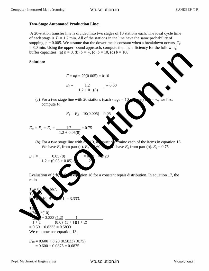
Two-Stage Automated Production Line:
A 20-station transfer line is divided into two stages of 10 stations each. The ideal cycle time of each stage is Tc = 1.2 min. All of the stations in the line have the same probability of stopping, p = 0.005. We assume that the downtime is constant when a breakdown occurs, Td = 8.0 min. Using the upper-bound approach, compute the line efficiency for the following buffer capacities: (a) b = 0, (b) b = �, (c) b = 10, (d) b = 100
Solution:
F = np = 20(0.005) = 0.10
E0 = 1.2 = 0.60 1.2 + 0.1(8)
(a) For a two stage line with 20 stations (each stage = 10 stations) & b = �, we firstcompute F:
F1 = F2 = 10(0.005) = 0.05
E� = E1 = E2 = 1.2 = 0.75 1.2 + 0.05(8)
(b) For a two stage line with b = 10, we must determine each of the items in equation 13.We have E0 from part (a). E0 = 0.60. And we have E2 from part (b). E2 = 0.75
D'1 = 0.05 (8) = 0.40 = 0.20 1.2 + (0.05 + 0.05) (8) 2.0
Evaluation of h(b) is from equation 18 for a constant repair distribution. In equation 17, the ratio
Td = 8.0 = 6.667. Tc 1.2 For b = 10, B = 1 & L = 3.333.
Thus, h(b) = h(10) = 1 + 3.333 (1.2) 1
1 + 1 (8.0) (1 + 1)(1 + 2) = 0.50 + 0.8333 = 0.5833 We can now use equation 13:
E10 = 0.600 + 0.20 (0.5833) (0.75) = 0.600 + 0.0875 = 0.6875
Computer Integrated Manufacturing SANDEEP T R
Dept. Mechanical Engineering Vtusolution.in
Vtusolution.in
Vtusolution.in
vtuso
lution
.in
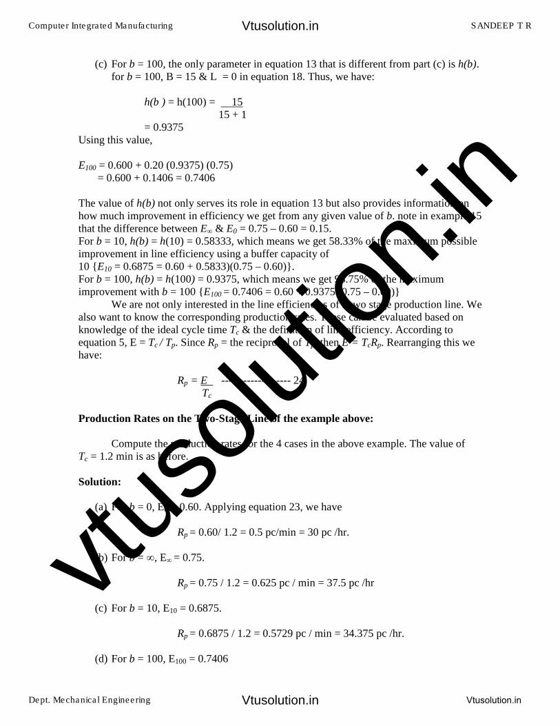
(c) For b = 100, the only parameter in equation 13 that is different from part (c) is h(b).for b = 100, B = 15 & L = 0 in equation 18. Thus, we have:
h(b ) = h(100) = 15 15 + 1
= 0.9375 Using this value,
E100 = 0.600 + 0.20 (0.9375) (0.75) = 0.600 + 0.1406 = 0.7406
The value of h(b) not only serves its role in equation 13 but also provides information on how much improvement in efficiency we get from any given value of b. note in example 15 that the difference between E� & E0 = 0.75 – 0.60 = 0.15. For b = 10, h(b) = h(10) = 0.58333, which means we get 58.33% of the maximum possible improvement in line efficiency using a buffer capacity of 10 {E10 = 0.6875 = 0.60 + 0.5833)(0.75 – 0.60)}. For b = 100, h(b) = h(100) = 0.9375, which means we get 93.75% of the maximum improvement with b = 100 {E100 = 0.7406 = 0.60 + 0.9375 (0.75 – 0.60)}
We are not only interested in the line efficiencies of a two stage production line. We also want to know the corresponding production rates. These can be evaluated based on knowledge of the ideal cycle time Tc & the definition of line efficiency. According to equation 5, E = Tc / Tp. Since Rp = the reciprocal of Tp, then E = TcRp. Rearranging this we have:
Rp = E ------------------- 24
Tc
Production Rates on the Two-Stage Line of the example above:
Compute the production rates for the 4 cases in the above example. The value of Tc = 1.2 min is as before.
Solution:
(a) For b = 0, E0 = 0.60. Applying equation 23, we have
Rp = 0.60/ 1.2 = 0.5 pc/min = 30 pc /hr.
(b) For b = �, E� = 0.75.
Rp = 0.75 / 1.2 = 0.625 pc / min = 37.5 pc /hr
(c) For b = 10, E10 = 0.6875.
Rp = 0.6875 / 1.2 = 0.5729 pc / min = 34.375 pc /hr.
(d) For b = 100, E100 = 0.7406
Computer Integrated Manufacturing SANDEEP T R
Dept. Mechanical Engineering Vtusolution.in
Vtusolution.in
Vtusolution.in
vtuso
lution
.in
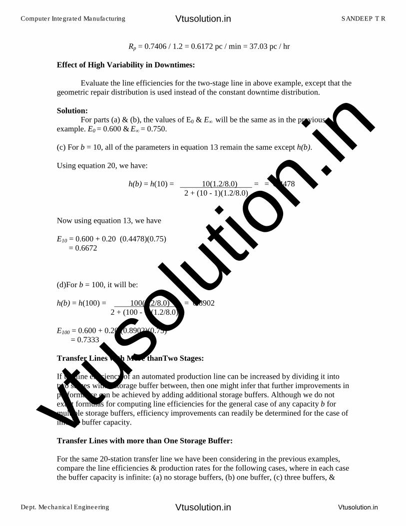
Rp = 0.7406 / 1.2 = 0.6172 pc / min = 37.03 pc / hr
Effect of High Variability in Downtimes:
Evaluate the line efficiencies for the two-stage line in above example, except that the geometric repair distribution is used instead of the constant downtime distribution.
Solution:
For parts (a) & (b), the values of E0 & E� will be the same as in the previous example. E0 = 0.600 & E� = 0.750.
(c) For b = 10, all of the parameters in equation 13 remain the same except h(b).
Using equation 20, we have:
h(b) = h(10) = 10(1.2/8.0) = = 0.4478 2 + (10 - 1)(1.2/8.0)
Now using equation 13, we have
E10 = 0.600 + 0.20 (0.4478)(0.75) = 0.6672
(d)For b = 100, it will be:
h(b) = h(100) = 100(1.2/8.0) = 0.8902 2 + (100 - 1)(1.2/8.0)
E100 = 0.600 + 0.20 (0.8902)(0.75) = 0.7333
Transfer Lines with More thanTwo Stages:
If the line efficiency of an automated production line can be increased by dividing it into two stages with a storage buffer between, then one might infer that further improvements in performance can be achieved by adding additional storage buffers. Although we do not exact formulas for computing line efficiencies for the general case of any capacity b for multiple storage buffers, efficiency improvements can readily be determined for the case of infinite buffer capacity.
Transfer Lines with more than One Storage Buffer:
For the same 20-station transfer line we have been considering in the previous examples, compare the line efficiencies & production rates for the following cases, where in each case the buffer capacity is infinite: (a) no storage buffers, (b) one buffer, (c) three buffers, &
Computer Integrated Manufacturing SANDEEP T R
Dept. Mechanical Engineering Vtusolution.in
Vtusolution.in
Vtusolution.in
vtuso
lution
.in
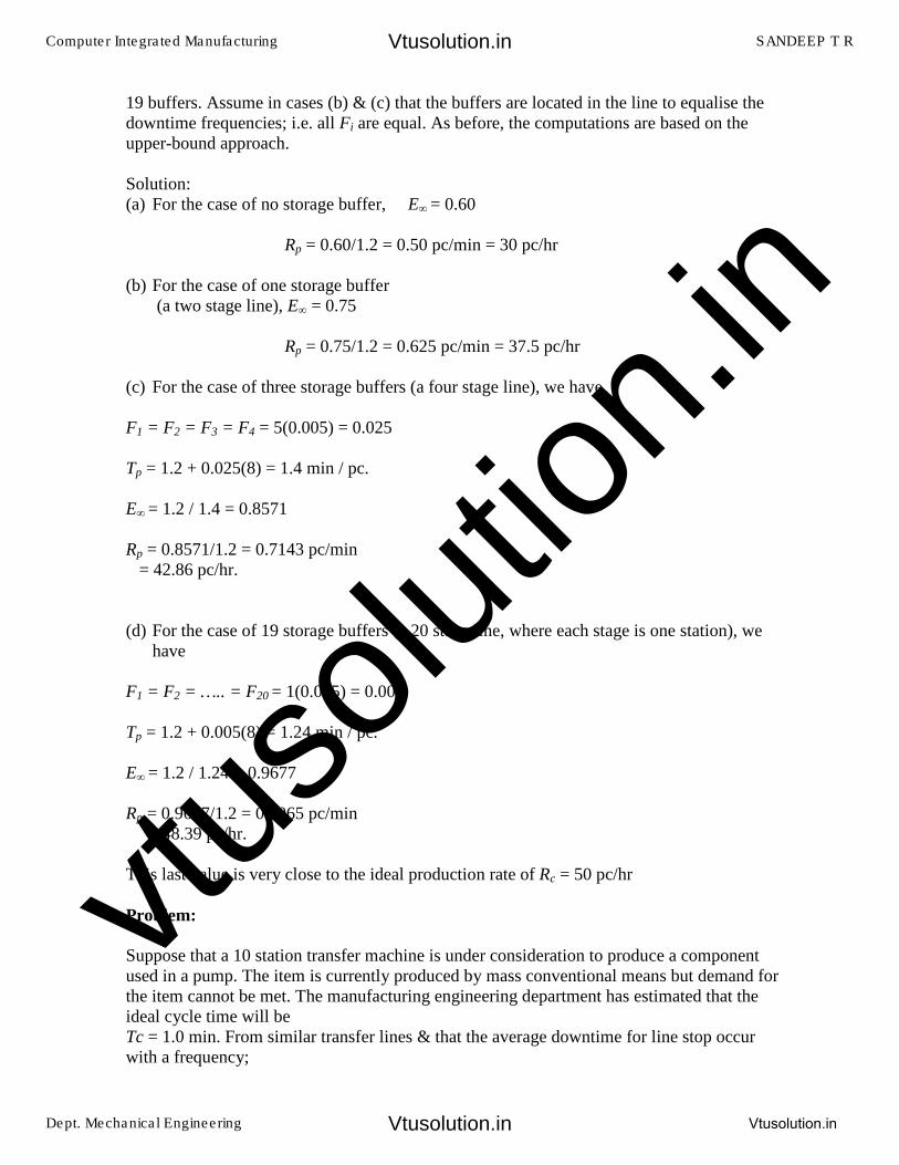
19 buffers. Assume in cases (b) & (c) that the buffers are located in the line to equalise the downtime frequencies; i.e. all Fi are equal. As before, the computations are based on the upper-bound approach.
Solution: (a) For the case of no storage buffer, E� = 0.60
Rp = 0.60/1.2 = 0.50 pc/min = 30 pc/hr
(b) For the case of one storage buffer(a two stage line), E� = 0.75
Rp = 0.75/1.2 = 0.625 pc/min = 37.5 pc/hr
(c) For the case of three storage buffers (a four stage line), we have
F1 = F2 = F3 = F4 = 5(0.005) = 0.025
Tp = 1.2 + 0.025(8) = 1.4 min / pc.
E� = 1.2 / 1.4 = 0.8571
Rp = 0.8571/1.2 = 0.7143 pc/min = 42.86 pc/hr.
(d) For the case of 19 storage buffers (a 20 stage line, where each stage is one station), wehave
F1 = F2 = ….. = F20 = 1(0.005) = 0.005
Tp = 1.2 + 0.005(8) = 1.24 min / pc.
E� = 1.2 / 1.24 = 0.9677
Rp = 0.9677/1.2 = 0.8065 pc/min = 48.39 pc/hr.
This last value is very close to the ideal production rate of Rc = 50 pc/hr
Problem:
Suppose that a 10 station transfer machine is under consideration to produce a component used in a pump. The item is currently produced by mass conventional means but demand for the item cannot be met. The manufacturing engineering department has estimated that the ideal cycle time will be Tc = 1.0 min. From similar transfer lines & that the average downtime for line stop occur with a frequency;
Computer Integrated Manufacturing SANDEEP T R
Dept. Mechanical Engineering Vtusolution.in
Vtusolution.in
Vtusolution.in
vtuso
lution
.in
F = 0.10 breakdown/cycle & the average downtime per line stop will be 6.0 min. The scrap rate for the current conventional processing method is 5% & this is considered a good estimate for a transfer line. The starting costing for the component costs Rs. 1.50 each & it will cost Rs 60.00 / hr or Rs 1 / min to operate the transfer line. Cutting tools are estimated to cost Rs 0.15/ work part. Compute the following measures of line performance given the foregoing data.
(a) Production rate(b) Number of hours required to meet a demand of 1500 units/week.(c) Line efficiency(d) Cost per unit produced.
Problem:
If a line has 20 work stations each with a probability of breakdown of 0.02, the cycle time of the line is 1 min & each time a breakdown occurs, it takes exactly 5 minutes to repair. The line is to be divided into two stages by a storage buffer so that each stage will consist of 10 stations. Compute the efficiency of the two stage line for various buffer capacities.
Solution:
Let us compute the efficiency of the line with no buffer
F = np = 20(0.02) =0.4 Eo = 1.0 = 0.20
1.0+0.4(10)
Next dividing the line into equal stages by a buffer zone of infinite capacity each stage would have an efficiency given by F1 = F2 = 10 (0.02) = 0.2 E1 = E2 = Tc = 1.0 = 0.333
Tc + (F1+F2)Td 1.0+ 0.2(10)
d) The cost per product can be computed except that we must account for the scrap rate.Cpc = 1 (1.50+1.00 x 1.60 + 0.15) = Rs.3.42/good unit
0.95
The Rs.3.42 represents the average cost per acceptable product under the assumption that we are discarding the 5% bad units with no salvage value and no disposal cost. Suppose that we could repair these parts at a cost of Rs.5.00/unit. To compute the cost per piece the repair cost would be added to other components. Cpc = 1.50 + 1.00 x 1.60 + 0.15 + 0.05 (5.00) = Rs. 3.50/unit. The policy of scrapping the 5% defects ,yields a lower cost per unit rather than repairing them.
Computer Integrated Manufacturing SANDEEP T R
Dept. Mechanical Engineering Vtusolution.in
Vtusolution.in
Vtusolution.in
vtuso
lution
.in
Problem:
An eight station rotary indexing machine operates with an ideal cycle time of 20 secs. The frequency of line stop occurrences is 0.06 stop / cycle on the average. When a stop occurs it takes an average of 3 min to make repairs. Determine the following:
1. Average production time 3. Line efficiency2. Proportion of downtime 4. Average production rate
Solution Tp = Tc + F ( Td)
= 0.33 + 0.06(3) = 0.5133 minutes.
Rp = 1 = 1.94 pieces /minutes 0.5133
Line efficiency = Tc = 0.333 = 0.491 Tp 0.51
Proportion of downtime can be calculated by D = F Td = 0.06(3) = 0.35 Tp 0.5133
Partial Automation:
Many assembly lines in industry contain a combination of automated & manual work stations. These cases of partially automated production lines occur for two main reasons:
1. Automation is introduced gradually on an existing manual line. Suppose thatdemand for the product made on a manually operated line increases, & it is desiredto increase production & reduce labour costs by automating some or all of thestations. The simpler operations are automated first, & the transition toward a fullyautomated line is accomplished over a long period of time. Meanwhile, the lineoperates as a partially automated system.
2. Certain manual operations are too difficult or too costly to automate. Therefore,when the sequence of workstations is planned for the line, certain stations aredesigned to be automated, whereas the others are designed as manual stations.
Examples of operations that might be too difficult to automate are assembly procedures or processing steps involving alignment, adjustment, or fine-tuning of the work unit. These operations often require special human skills and/or senses to carry out. Many inspection procedures also fall into this category. Defects in a product or a part that can be easily perceived by a human inspector are sometimes extremely difficult to identify by an automated inspection device. Another problem is that the automated inspection device can only check for the defects for which it was designed, whereas a human inspector is capable of sensing a variety of unanticipated imperfections & problems.
To analyze the performance of a partially automated production line, we build on our previous analysis & make the following assumptions: 1. Workstations perform either processing or assembly operations;
Computer Integrated Manufacturing SANDEEP T R
Dept. Mechanical Engineering Vtusolution.in
Vtusolution.in
Vtusolution.in
vtuso
lution
.in
2. Processing & assembly times at automated stations are constant, though notnecessarily equal at all stations;
3. Synchronous transfer of parts;4. No internal buffer storage ;5. The upper bound approach is applicable &6. Station breakdowns occur only at automated stations.Breakdowns do not occur at manual workstations because the human workers areflexible enough, we assume, to adapt to the kinds of disruptions & malfunctions thatwould interrupt the operation of an automated workstation. For example, if a humanoperator were to retrieve a defective part from the parts bin at the station, the partwould immediately be discarded & replaced by another without much lost time. Ofcourse, this assumption of human adaptability is not always correct, but our analysisis based on it.
The ideal cycle time Tc is determined by the slowest stations on the line, which is generally one of the manual stations. If the cycle time is in fact determined by a manual station, then Tc will exhibit a certain degree of variability simply because there is a random variation in any repetitive human activity. However, we assume that the average Tc remains constant over time. Given our assumption that breakdowns occur only at automated stations, let na = the number of automated stations & Td = average downtime per occurrence. For the automated stations that perform processing operations, let pi = the probability (frequency) of breakdowns per cycle; & for automated stations that perform assembly operations, let qi & mi equal, respectively, the defect rate & probability that the defect will cause station i to stop. We are now in a position to define the average actual production time:
Tp = Tc + � piTd --------- 25
i�na
where the summation applies to the na automated stations only. For those automated stations that perform assembly operations in which a part is added,
pi = miqi
If all pi, mi, & qi are equal, respectively to p, m, & q, then the preceding equations reduce to the following:
Tp = Tc +napTd ---------- 26
and p = mq for those stations that perform assembly consisting of the addition of a part.
Given that na is the number of automated stations, then nw = the number of stations operated by manual workers, & na + nw = n, where n = the total station count. Let Casi = cost to operate the automatic workstation i ($ / min), Cwi = cost to operated manual workstation i ($ / min), Cat = cost to operate the automatic transfer mechanism. Then the total cost to operate the line is given by:
Co = Cat + �Casi + �Cwi -------- 27 i�na i�nw
Computer Integrated Manufacturing SANDEEP T R
Dept. Mechanical Engineering Vtusolution.in
Vtusolution.in
Vtusolution.in
vtuso
lution
.in

where Co = cost or operating the partially automated production system ($ / min). For all Casi = Cas & all Cwi = Cw, then Co = Cat + naCas + nwCw -------- 28
Now the total cost per unit produced on the line can be calculated as follows:
Cpc = Cm + CoTp + Ct ---------- 29 Pap
Where Cpc = cost per good assembly ($ / pc), Cm = cost of materials & components being processed & assembled on the line ($ / pc), Co = cost of operating the partially automated production system by either of the equations 27 or 28 ($ / min), Tp = average actual production time (min / pc), Ct = any cost of disposable tooling ($ / pc), & Pap = proportion of good assemblies.
Problem On Partial Automation:
It has been proposed to replace one of the current manual workstations with an automatic work head on a ten-station production line. The current line has six automatic stations & four manual stations. Current cycle time is 30 sec. The limiting process time is at the manual station that is proposed for replacement. Implementing the proposal would allow the cycle time to be reduced to 24 sec. The new station would cost $0.20/min. Other cost data: Cw = $0.15/min, Cas = $0.10/min, & Cat = $0.12/min. Breakdowns occur at each automated station with a probability p = 0.01. The new automated station is expected to have the same frequency of breakdowns. Average downtime per occurrence Td = 3.0min, which will be unaffected by the new station. Material costs & tooling costs will be neglected in the analysis. It is desired to compare the current line with the proposed change on the basis of production rate & cost per piece. Assume a yield of 100% good product.
Solution:
For the current line, Tc = 30 sec = 0.50min.
Tp = 0.50 + 6(0.01)(3.0) = 0.68 min. Rp = 1/0.68 = 1.47 pc/min = 88.2pc/hr Co = 0.12 + 4(0.15) + 6 (0.10) = $1.32 / min
Cpc = 1.32 (0.68) = $0.898 / pc
For the proposed line, Tc = 24 sec = 0.4 min. Rp = 1/0.61 = 1.64 pc/min = 98.4pc/hr Co = 0.12 + 3(0.15)+ 6(0.10)+ 1(0.20)
Computer Integrated Manufacturing SANDEEP T R
Dept. Mechanical Engineering Vtusolution.in
Vtusolution.in
Vtusolution.in
vtuso
lution
.in
= $1.37/min Cpc = 1.67(0.61) = $0.836 / pc
Even though the line would be more expensive to operate per unit time, the proposed chage would increase production rate & reduced piece cost.
Storage Buffers:
The preceding analysis assumes no buffer storage between stations. When the automated portion of the line breaks down, the manual stations must also stop for lack of work parts (either due to starving or blocking, depending on where the manual stations are located relative to the automated stations). Performance would be improved if the manual stations could continue to operate even when the automated stations stop for a temporary downtime incident. Storage buffers located before & after the manual stations would reduce forced downtime at these stations.
Problem On Storage Buffers on a Partially Automated Line:
Considering the current line in the above example, suppose that the ideal cycle time for the automated stations on the current line Tc = 18 sec. The longest manual time is 30 sec. Under the method of operation assumed in the above example both manual & automated stations are out of action when a breakdown occurs at an automated station. Suppose that storage buffers could be provided for each operator to insulate them from breakdowns at automated stations. What effect would this have on production rate & cost per piece?
Solution:
Given Tc = 18sec = 0.3min, the average actual production time on the automated stations is computed as follows:
Tp = 0.30 + 6(0.01)(3.0) = 0.48min
Since this is less than the longest manual time of 0.50, the manual operation could work independently of the automated stations if storage buffers of sufficient capacity were placed before & after each manual station. Thus, the limiting cycle time on the line would be Tc = 30sec = 0.50 min, & the corresponding production rate would be:
Rp = Rc = 1/0.50 = 2.0pc/min = 120.0 pc/hr
Using the line operating cost from the previous example, Co = $1.32/min, we have a piece cost of
Cpc = 1.32 (0.50) = $0.66 / pc
Comparing with the previous example, we can see that a dramatic improvement in production rate & unit cost is achieved through the use of storage buffers.
Computer Integrated Manufacturing SANDEEP T R
Dept. Mechanical Engineering Vtusolution.in
Vtusolution.in
Vtusolution.in
vtuso
lution
.in

Problem On Partial Automation:
A partially automated production line has a mixture of three mechanized & three manual workstations. There are a total of six stations, & the ideal cycle time Tc = 1.0 min, which includes a transfer time Tr = 6 sec. Data on the six stations are listed in the following table. Cost of the transfer mechanism Cat = $0.10/min, cost to run each automated station Cas = $ 0.12/min, & labour cost to operate each manual station Cw = $ 0.17 /min. It has been proposed to substitute an automated station in place of station 5. The cost of this station is estimated at Cas5 = $ 0.25 / min, & its breakdown rate P5 = 0.02, but its process time would be only 30 sec, thus reducing the overall cycle time of the line from 1.0 min to 36 sec. Average downtime per breakdown of the current line as well as the proposed configuration is Td = 3.5 min. Determine the following for the current line & the proposed line: (a) production rate, (b) proportion uptime, & (c) cost per unit. Assume the line operates without storage buffers, so when an automated station stops, the whole line stops, including the manual stations. Also, in computing costs, neglect material & tooling costs.
Station Type Process Time (sec) pi
1 Manual 36 0
2 Automatic 15 0.01
3 Automatic 20 0.02
4 Automatic 25 0.01
5 Manual 54 0
6 Manual 33 0
Solution : Tc = 1.0 min Tp = 1.0 + 2(0.01)x3.5 + 1( 0.02) x 3.5 = 1.14 mins Rp = 1 = 0.877 pcs /min x 60 = 52.65 pcs / hr
1.14 Cp = 0.12 + 3(0.17) + 3(0.10) = $ 0.93/mins Cpc = 0.93x 1.14 = $1.062/piece For the proposed line Tc = 36 secs = 0.6 mins Tp = 0.6 + 2(0.01)3.5 + 2(0.02)3.5 = 0.81 mins Rp = 1.234 pieces / min = 74.07 pieces/hr Cp = 0.012 + 2(0.17) + 3(0.10) + 1(0.25) = $ 0.902/min Cpc = 0.90 x 0.81 mins = $ 0.73062/piece
Transfer of Work between Work Stations:
There are two basic ways in which the work (the subassembly that is being built up) is moved on the line between operator workstations.
1. Nonmechanical Lines. In this arrangement, no belt or conveyor is used to move the
parts between operator workstations. Instead, the parts are passed from station to
station by hand. Several problems result from this mode of operation:
� Starving at stations, where the operator has completed his or her work
but must wait for parts from the preceding station.
Computer Integrated Manufacturing SANDEEP T R
Dept. Mechanical Engineering Vtusolution.in
Vtusolution.in
Vtusolution.in
vtuso
lution
.in
� Blocking of stations, where the operator has completed his or her
work but must wait for the next operator to finish the task before
passing along the part.
As a result of these problems, the flow of work on a nonmechanical line is usually uneven. The cycle times vary, and this contributes to the overall irregularity. Buffer stocks of parts between workstations are often used to smooth out the production flow.
• Moving conveyor lines. These flow lines use a conveyor (e.g., a moving belt,
conveyor, chain-in-the-floor, etc.) to move the subassemblies between workstations.
The transport system can be continuous, intermittent (synchronous), or
asynchronous. Continuous transfer is most common in assembly lines, although
asynchronous transfer is becoming more popular. With the continuously moving
conveyor, the following problems can arise:
� Starving can occur as with non mechanical lines.
� Incomplete items are sometimes produced when the operator is
unable to finish the current part & the next part travels right by on the
conveyor. Blocking does not occur.
Again, buffer stocks are sometimes used to overcome these problems. Also stations overlaps can sometimes be allowed, where the worker is permitted to travel beyond the normal boundaries of the station in order to complete work.
In the moving belt line, it is possible to achieve a higher level of control over the production rate of the line. This is accomplished by means of the feed rate, which refers to the reciprocal of the time interval between work parts on the moving belt. Let fp denote this feed rate. It is measured in work pieces per time & depends on two factors: the speed with which the conveyor moves, & the spacing of work parts along the belt. Let Vc equal the conveyor speed (feet per minute or meters per second) & sp equal the spacing between parts on the moving conveyor (feet or meters per work piece). Then the feed rate is determined by
fp = Vc -------------- 1 Sp
To control the feed rate of the line, raw work parts are launched onto the line at regular intervals. As the parts flow along the line, the operator has a certain time period during which he or she begin work on each piece. Otherwise, the part will flow past the station. This time period is called the tolerance time Tt. It is determined by the conveyor speed & the length of the workstation. This length we will symbolize by Ls, & it is largely determined by the operator’s reach at the workstation. The tolerance time is therefore defined by
Tt = Ls ----------- 2 Vc
For example, suppose that the desired production rate on a manual flow line with moving conveyor were 60 units/h. this would necessitate a feed rate of 1 part/min. This could be achieved by a conveyor speed of 0.6m/min & a part spacing of 0.5m. (Other combinations of Vc & sp would also provide the same feed rate.) If the length of each workstation were 1.5m. the tolerance time available to the operators for each work piece
Computer Integrated Manufacturing SANDEEP T R
Dept. Mechanical Engineering Vtusolution.in
Vtusolution.in
Vtusolution.in
vtuso
lution
.in
would be 3 min. It is generally desirable to make the tolerance time large to compensate for worker process time variability.
Mode Variations:
In both nonmechanical lines & moving conveyor lines it is highly desirable to assign work to the stations so as to equalize the process or assembly times at the workstations. The problem is sometimes complicated by the fact that the same production line may be called upon to process more than one type of product. This complication gives rise to the identification of three flow line cases (and therefore three different types of line balancing problems).
The three production situations on flow lines are defined according to the product or products to be made on the line. Will the flow line be used exclusively to produce one particular model? Or, will it be used to produce several different models, & if so how will they be scheduled on line? There are three cases that can be defined in response to these questions:
1. Single-model line. This is a specialized line dedicated to the production of a singlemodel or product. The demand rate for the product is great enough that the line is devoted 100% of the time to the production of that product.
2. Batch-model line. This line is used for the production of two or more models. Eachmodel is produced in batches on the line. The models or products are usually similar in the sense of requiring a similar sequence of processing or assembly operations. It is for this reason that the same line can be used to produce the various models.
3. Mixed-model lines. This line is also used for the production of two or more models,but the various models are intermixed on the line so that several different models are being produced simultaneously rather than in batches. Automobile & truck assembly lines are examples of this case.
To gain a better perspective of the three cases, the reader might consider the following. In the case of the batch-model line, if the batch sizes are very large, the batch-model line approaches the case of the single-model line. If the batch sizes become very small (approaching a batch size of 1), the batch-model line approximates to the case of the mixed-model line.
In principle, the three cases can be applied in both manual flow lines & automated flow lines. However, in practice, the flexibility of human operators makes the latter two cases more feasible on the manual assembly line. It is anticipated that future automated lines will incorporate quick changeover & programming capabilities within their designs to permit the batch-model, & eventually the mixed-model, concepts to become practicable.
Achieving a balanced allocation of work load among stations of the line is a problem in all three cases. The problem is least formidable for the single-model case. For the batch-model line, the balancing problem becomes more difficult; & for the mixed-model case, the problem of line balancing becomes quite complicated.
In this chapter we consider only the single-model line balancing problem, although the same concepts & similar terminology & methodology apply for the batch & mixed model cases.
Computer Integrated Manufacturing SANDEEP T R
Dept. Mechanical Engineering Vtusolution.in
Vtusolution.in
Vtusolution.in
vtuso
lution
.in
The Line Balancing Problem:
In flow line production there are many separate & distinct processing & assembly operations to be performed on the product. Invariably, the sequence of processing or assembly steps is restricted, at least to some extent, in terms of the order in which the operations can be carried out. For example, a threaded hole must be drilled before it can be tapped. In mechanical fastening, the washer must be placed over the bolt before the nut can be turned & tightened. These restrictions are called precedence constraints in the language of line balancing. It is generally the case that the product must be manufactured at some specified production rate in order to satisfy demand for the product. Whether we are concerned with performing these processes & assembly operations on automatic machines or manual flow lines, it is desirable to design the line so as to satisfy all of the foregoing specifications as efficiently as possible.
The line balancing problem is to arrange the individual processing & assembly tasks at the workstations so that the total time required at each workstation is approximately the same. If the work elements can be grouped so that all the station times are exactly equal, we have perfect balance on the line & we can expect the production to flow smoothly. In most practical situations it is very difficult to achieve perfect balance. When the workstations times are unequal, the slowest station determines the overall production rate of the line.
In order to discuss the terminology & relationships in line balancing, we shall refer to the following example. Later, when discussing the various solution techniques, we shall apply the techniques to this problem.
Computer Integrated Manufacturing SANDEEP T R
Dept. Mechanical Engineering Vtusolution.in
Vtusolution.in
Vtusolution.in
vtuso
lution
.in
UNIT 4 :
Minimum Rational Work Element:
In order to spread the job to be done on the line among its stations, the job must be divided
into its component tasks. The minimum rational work elements are the smallest practical indivisible
tasks into which the job can be divided. These work elements cannot be subdivided further. For
example, the drilling of a hole would normally be considered as a minimum rational work element. In
manual assembly, when two components are fastened together with a screw & nut, it would be
reasonable for these activities to be taken together. Hence, this assembly task would constitute a
minimum rational work element. We can symbolize the time required to carry out this minimum
rational work element Tej, where j is used to identify the element out of the ne elements that make up
the total work or job. For instance, the element time Tej, for element 1 in the table above is 0.2 min.
The time Tej of a work element is considered a constant rather than a variable. An automatic
work head most closely fits this assumption, although the processing time could probably be altered
by making adjustments in the station. In a manual operation, the time required to perform a work
element will, in fact, vary from cycle to cycle.
Another assumption implicit in the use of Te values is that they are additive. The time to
perform two work elements is the sum of the times of the individual elements. In practice, this might
not be true. It might be that some economy of motion could be achieved by combining two work
elements at one station, thus violating the additivity assumption
Problem:
A new small electrical appliance is to be assembled on a production flow line. The total job of
assembling the product has been divided into minimum rational work elements. The industrial
engineering department has developed time standards based on previous similar jobs. This
information is given in the table below. In the right hand column are the immediate predecessors for
each element as determined by precedence requirements. Production demand will be 120,000
units/yr. At 50 weeks/yr & 40 h/week, this reduces to an output from the line of 60 units/h or 1
unit/min.
Computer Integrated Manufacturing SANDEEP T R
Dept. Mechanical Engineering Vtusolution.in
Vtusolution.in
Vtusolution.in
vtuso
lution
.in

No. Element description Tej Must be preceded by:
1 Place frame on work holder & clamp 0.2 --------
2 Assemble plug, grommet to power cord 0.4 --------
3 Assemble brackets to frame 0.7 1
4 Wire power cord to motor 0.1 1.2
5 Wire power to switch 0.3 2
6 Assemble mechanism plate to bracket 0.11 3
7 Assemble blade to bracket 0.32 3
8 Assemble motor to brackets 0.6 3, 4
9 Align blade & attach to motor 0.27 6, 7, 8
10 Assemble switch to motor bracket 0.38 5, 8
11 Attach cover, inspect, & test 0.5 9, 10
12 Place in tote pan for packing 0.12 11
Total Work Content:
This is the aggregate of all the work elements to be done on the line. Let Twc be the time
required for the total work content. Hence,
nc Twc = � Tej ------------- 3
j=1
For the example, Twc = 4.00 min.
Workstation Process Time:
A workstation is a location along the flow line where work is performed, either manually or
by some automatic device. The work performed at the station consists of one or more of the
individual work elements & the time required is the sum of the times of the work elements done at the
station. We use Tsi to indicate the process time at station i of an n- station line. It should be clear that
the sum of the station process times should equal the sum of the work element times.
n ne
� Tsi = � Tej ----------- 4
i=1 j=1
Computer Integrated Manufacturing SANDEEP T R
Dept. Mechanical Engineering Vtusolution.in
Vtusolution.in
Vtusolution.in
vtuso
lution
.in
Cycle Time:
This is the ideal or theoretical cycle time of the flow line, which is the time interval between
parts coming off the line. The design value of Tc would be specified according to the required
production rate to be achieved by the flow line. Allowing for downtime on the line, the value of Tc
must meet the following requirement:
Tc � E -------------- 5
Rp
Where E is the line efficiency & Rp the required production rate.
The line efficiency of an automated line will be somewhat less than 100%. For a manual line,
where mechanical malfunctions are less likely the efficiency will be closer to 100%.
In the above example, the required production rate is 60 units/h or 1 unit/min. at a line
efficiency of 100%, the value Tc of would be 1.0 min. At efficiencies less than 100%, the ideal cycle
time must be reduced (or what is the same thing, the ideal production rate Rc must be increased) to
compensate for the downtime.
The minimum possible value Tc of is established by the bottleneck station, the one with the
largest of Ts. That is
Tc � max Tsi ------------ 6
If Tc = maxTsi, there will be idle time at all stations whose Ts values are less than Tc.
Finally, since the station times are comprised of element times,
Tc � Tej (for all j =1, 2, …….ne) --------- 7
This equation states the obvious: that the cycle time must be greater than or equal to any of
the element times.
Computer Integrated Manufacturing SANDEEP T R
Dept. Mechanical Engineering Vtusolution.in
Vtusolution.in
Vtusolution.in
vtuso
lution
.in
Precedence Constraints:
These are also referred to as “technological sequencing requirements”. The order in which the
work elements can be accomplished is limited at least to some extent. In the problem above, the
switch must be mounted onto the motor bracket before the cover of the appliance can be attached.
The right hand column in the table above gives a complete listing of the precedence constraints for
assembling the hypothetical electrical appliance. In nearly every processing or assembly job, there are
precedence requirements that restrict the sequence in which the job can be accomplished.
In addition to the precedence constraints described above, there may be other types of
constraints on the line balancing solution. These concern the restrictions on the arrangement of the
stations rather than the sequence of work elements. The first is called a zoning constraint. A zoning
constraint may be either a positive constraint or a negative constraint. A positive zoning constraint
means that certain work elements should be placed near each other, preferably at the same
workstation. For example, all the spray-painting elements should be performed together since a
special semienclosed workstation has to be utilized. A negative zoning constraint indicates that work
elements might interfere with one another & should therefore not be located in close proximity. As an
illustration, a work element requiring fine adjustments or delicate coordination should not be located
near a station characterized by loud noises & heavy vibrations.
Another constraint on the arrangement of workstations is called a position constraint. This
would be encountered in the assembly of large products such as automobiles or major appliances. The
product is too large for one worker to perform work on both sides. Therefore, for the sake of
facilitating the work, operators are located on both sides of the flow line. This type of situation is
referred to as a position constraint.
In the example there are no zoning constraints or position constraints given. The line
balancing methods are not equipped to deal with these constraints conveniently. However, in real-life
situations, they may constitute a significant consideration in the design of the flow line.
Precedence Diagram:
This is a graphical representation of the sequence of work elements as defined by the
precedence constraints. It is customary to use nodes to symbolize the work elements, with arrows
connecting the nodes to indicate the order in which the elements must be performed. Elements that
must be done first appear as nodes at the left of the diagram. Then the sequence of processing and/or
assembly progresses to the right. The element times are recorded above each node for convenience.
Computer Integrated Manufacturing SANDEEP T R
Dept. Mechanical Engineering Vtusolution.in
Vtusolution.in
Vtusolution.in
vtuso
lution
.in
Balance Delay:
Sometimes also called balancing loss, this is a measure of the line inefficiency which results
from idle time due to imperfect allocation of work among stations. It is symbolized as d & can be
computed for the flow line as follows:
d = nTc – Twc ---------- 8
nTc
The balance delay is often expressed as a percent rather than as a decimal fraction in Eq. 8.
The balance delay should not be confused with the proportion downtime, D, of an automated
flow line. D is a measure of the inefficiency that results from line stops. The balance delay measures
the inefficiency from imperfect line balancing.
Considering the data given in the previous problem, the total work content Twc = 4.00 min.
We shall assume that Tc = 1.0 min. If it were possible to achieve perfect balance with n = 4
workstations, the balance delay would be
d = 4(1.0) – 4.0 = 0
4(1.0)
If the line could only be balanced with n = 5 stations for the 1.0 min cycle, the balance delay would be
d = 5(1.0) – 4.0 = 0.20 or 20%
5(1.0)
Both of these solutions provide the same theoretical production rate. However, the second solution is less efficient because an additional workstation, & therefore an additional assembly operator, is required. One possible way to improve the efficiency of the five station line is to decrease the cycle time Tc. To illustrate, suppose that the line could be balanced at a cycle time of Tc = 0.80 min. The corresponding measure of inefficiency would be
d = 5(0.80) – 4.0 = 0
5(0.80)
This solution (if it were possible) would yield a perfect balance. Although five workstations are
required, the theoretical production rate would be Rc = 1.25 units/min, an increase over the production
rate capability of the four-station line. The reader can readily perceive that there are many
combinations of n & Tc that will produce a theoretically perfect balance. Each combination will give a
different production rate. In general, the balance delay d will be zero for any values n & Tc that satisfy
the relationship
nTc = Twc ------------- 9
Computer Integrated Manufacturing SANDEEP T R
Dept. Mechanical Engineering Vtusolution.in
Vtusolution.in
Vtusolution.in
vtuso
lution
.in
Unfortunately, because of precedence constraints & because the particular values of Tc usually do not
permit it, perfect balance might not be achievable for every nTc combinations that equals the total
work content time. In other words, the satisfaction of Eq. 9 is a necessary condition for perfect
balance, but not a sufficient condition.
As indicated by Eq 5, the desired maximum value of Tc is specified by the production rate
required of the flow line. Therefore Eq 9 can be cast in a different form to determine the theoretical
minimum number of workstations required to optimize the balance delay for a specified Tc. Since n
must be an integer, we can state:
minimum n is the smallest integer�Twc --- 10
Tc
Applying this rule to our example with
Twc = 4.0 min & Tc = 1.0 min, the minimum n = 4 stations.
Problem:1
A new small electrical appliance is to be assembled on a production flow line. The total job of
assembling the product has been divided into minimum rational work elements. The industrial
engineering department has developed time standards based on previous similar jobs. This
information is given in the table below. In the right hand column are the immediate predecessors for
each element as determined by precedence requirements. Production demand will be 120,000
units/yr. At 50 weeks/yr & 40 h/week, this reduces to an output from the line of 60 units/h or 1
unit/min.
No Element Description Tek (mins) Must be preceded by
1 Place frame on work holder & clamp 0.2 ----------------
2 Assemble plug, grommet to power cord 0.4 --------------------
3 Assemble brackets to frame 0.7 1
4 Wire power cord to motor 0.1 1 ,2
5 Wire power to switch 0.3 2
6 Assemble mechanism plate to bracket 0.11 3
7 Assemble blade to bracket 0.32 3
8 Assemble motor to brackets 0.6 3 , 4
9 Align blade & attach to motor 0.27 6 , 7 , 8
10 Assemble switch to motor bracket 0.38 5 , 8
11 Attach cover, inspect, & test 0.5 9 , 10
12 Place in tote pan for packing 0.12 11
Computer Integrated Manufacturing SANDEEP T R
Dept. Mechanical Engineering Vtusolution.in
Vtusolution.in
Vtusolution.in
vtuso
lution
.in
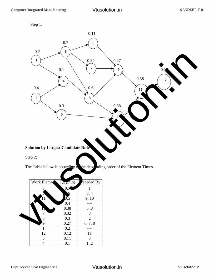
Step 1:
0.11
0.7
0.2
0.32 0.27
0.1 0.12
0.38
0.4 0.6
0.3 0.38
Solution by Largest Candidate Rule
Step 2:
The Table below is according to the descending order of the Element Times.
Work Element Tek (min) Preceded By
3 0.7 1
8 0.6 3, 4
11 0.5 9, 10
2 0.4 ----
10 0.38 5 ,8
7 0.32 3
5 0.3 2
9 0.27 6, 7, 8
1 0.2 ----
12 0.12 11
6 0.11 3
4 0.1 1 ,2
1
12
11
10
4
2
3
5
8
8
7
7
9
6
6
Computer Integrated Manufacturing SANDEEP T R
Dept. Mechanical Engineering Vtusolution.in
Vtusolution.in
Vtusolution.in
vtuso
lution
.in
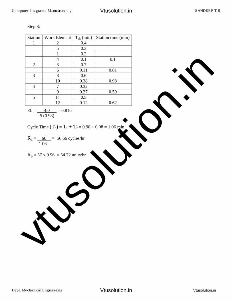
Step 3:
Eb = 4.0 = 0.816 5 (0.98)
Cycle Time (Tc) = Ts + Tr = 0.98 + 0.08 = 1.06 min
Rc = 60 = 56.66 cycles/hr 1.06
Rp = 57 x 0.96 = 54.72 units/hr
Station Work Element Tek (min) Station time (min)
1 2 0.4
5 0.3
1 0.2
4 0.1 0.1
2 3 0.7
6 0.11 0.81
3 8 0.6
10 0.38 0.98
4 7 0.32
9 0.27 0.59
5 11 0.5
12 0.12 0.62
Computer Integrated Manufacturing SANDEEP T R
Dept. Mechanical Engineering Vtusolution.in
Vtusolution.in
Vtusolution.in
vtuso
lution
.in
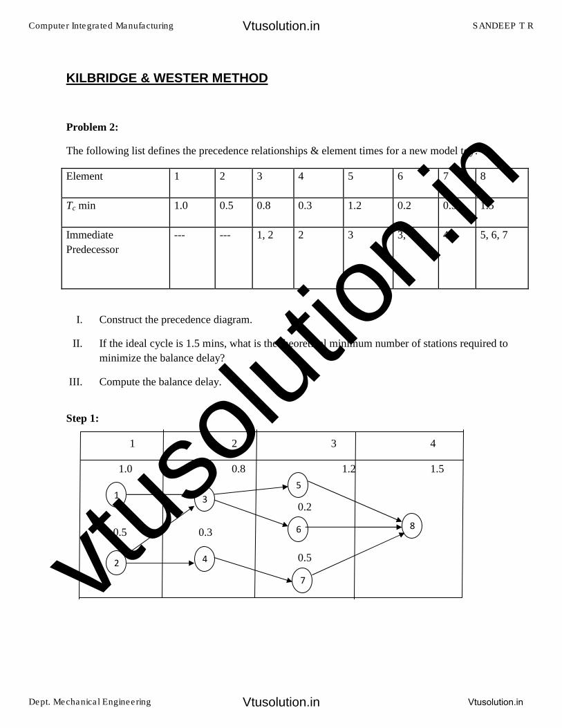
KILBRIDGE & WESTER METHOD
Problem 2:
The following list defines the precedence relationships & element times for a new model toy:
Element 1 2 3 4 5 6 7 8
Tc min 1.0 0.5 0.8 0.3 1.2 0.2 0.5 1.5
Immediate
Predecessor
--- --- 1, 2 2 3 3, 4 4 5, 6, 7
I. Construct the precedence diagram.
II. If the ideal cycle is 1.5 mins, what is the theoretical minimum number of stations required to
minimize the balance delay?
III. Compute the balance delay.
Step 1:
1 2 3 4
1.0 0.8 1.2 1.5
0.2
0.5 0.3
0.5
1
2
3
4
5
6 8
7
Computer Integrated Manufacturing SANDEEP T R
Dept. Mechanical Engineering Vtusolution.in
Vtusolution.in
Vtusolution.in
vtuso
lution
.in
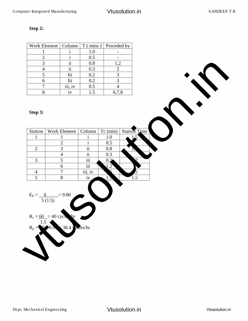
Step 2:
Step 3:
Eb = 6 = 0.80 5 (1.5)
Rc = 60 = 40 cycles/hr 1.5
Rp = 40 x 0.96 = 38.4 pieces/hr
Work Element Column T ( mins ) Preceded by
1 i 1.0 -
2 i 0.5 -
3 ii 0.8 1,2
4 ii 0.3 2
5 Iii 0.2 3
6 Iii 0.2 3
7 iii, iv 0.5 4
8 iv 1.5 6,7,8
Station Work Element Column Tc (min) Station Time
1 1 i 1.0 1.5
2 i 0.5
2 3 ii 0.8 1.3
4 ii 0.3
3 5 iii 0.2 1.2
6 iii 1.2
4 7 iii, iv 0.5 0.5
5 8 iv 1.5 1.5
Computer Integrated Manufacturing SANDEEP T R
Dept. Mechanical Engineering Vtusolution.in
Vtusolution.in
Vtusolution.in
vtuso
lution
.in
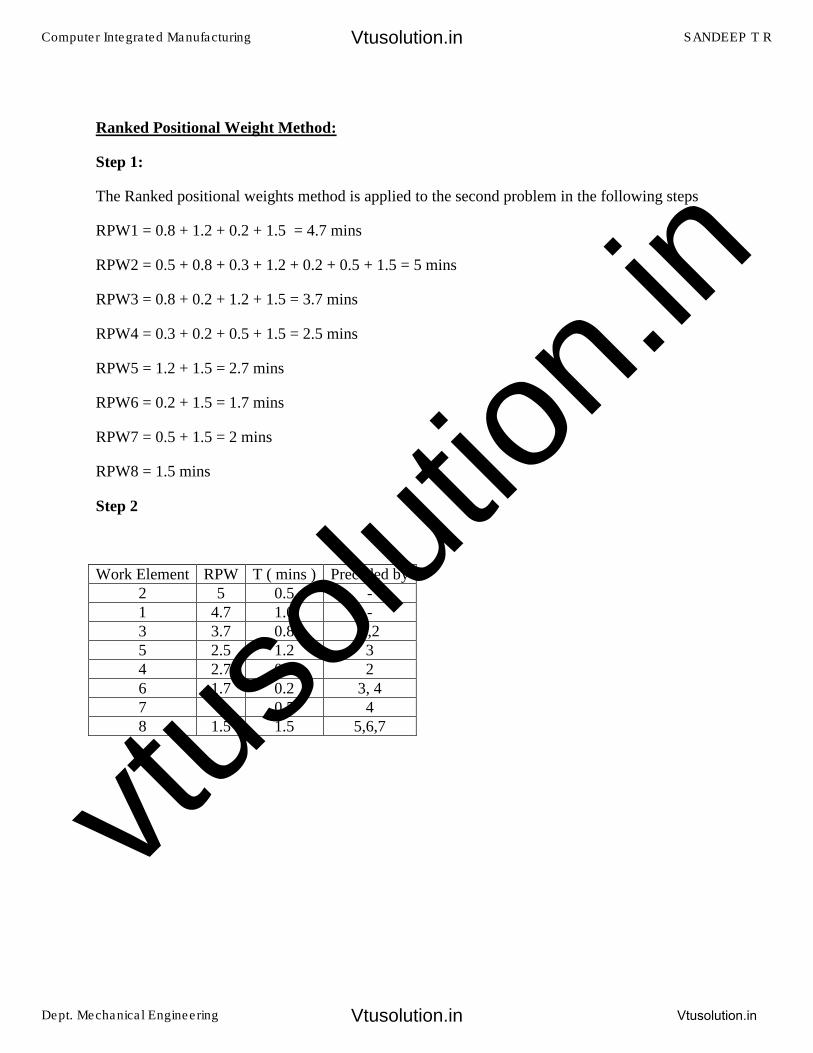
Ranked Positional Weight Method:
Step 1:
The Ranked positional weights method is applied to the second problem in the following steps
RPW1 = 0.8 + 1.2 + 0.2 + 1.5 = 4.7 mins
RPW2 = 0.5 + 0.8 + 0.3 + 1.2 + 0.2 + 0.5 + 1.5 = 5 mins
RPW3 = 0.8 + 0.2 + 1.2 + 1.5 = 3.7 mins
RPW4 = 0.3 + 0.2 + 0.5 + 1.5 = 2.5 mins
RPW5 = 1.2 + 1.5 = 2.7 mins
RPW6 = 0.2 + 1.5 = 1.7 mins
RPW7 = 0.5 + 1.5 = 2 mins
RPW8 = 1.5 mins
Step 2
Work Element RPW T ( mins ) Preceded by
2 5 0.5 -
1 4.7 1.0 -
3 3.7 0.8 1,2
5 2.5 1.2 3
4 2.7 0.3 2
6 1.7 0.2 3, 4
7 2 0.5 4
8 1.5 1.5 5,6,7
Computer Integrated Manufacturing SANDEEP T R
Dept. Mechanical Engineering Vtusolution.in
Vtusolution.in
Vtusolution.in
vtuso
lution
.in
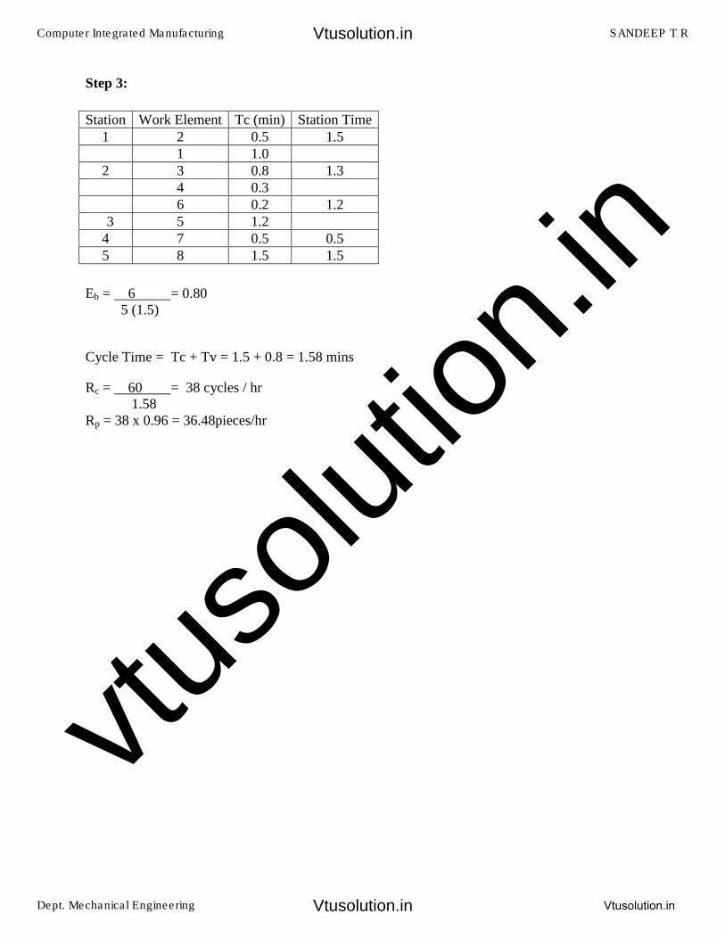
Step 3:
Eb = 6 = 0.80 5 (1.5)
Cycle Time = Tc + Tv = 1.5 + 0.8 = 1.58 mins
Rc = 60 = 38 cycles / hr 1.58
Rp = 38 x 0.96 = 36.48pieces/hr
Station Work Element Tc (min) Station Time
1 2 0.5 1.5
1 1.0
2 3 0.8 1.3
4 0.3
6 0.2 1.2
3 5 1.2
4 7 0.5 0.5
5 8 1.5 1.5
Computer Integrated Manufacturing SANDEEP T R
Dept. Mechanical Engineering Vtusolution.in
Vtusolution.in
Vtusolution.in
vtuso
lution
.in
UNIT-5:
AUTOMATED ASSSEMBLY SYSTEMS
Automated Assembly Systems
Assembly involves the joining together of two or more separate parts to form new
entity which may be assembly or subassembly.
Automated assembly refers to the use of mechanized and automated devices to
perform the various functions in an assembly line or cell.
Automated assembly system performs a sequence of automated operations to
combine multiple components in to a single entity which can be a final product or
sub assembly.
Automated assembly technology should be considered when the following
condition exists.
� High product demand
� Stable product design
� The assembly consists of no more than a limited number of components.
� The product is designed for automated assembly.
Automated assembly system involves less investment compared to transfer lines
because
1. Work part produced are smaller in size compared to transfer lines.
2. Assembly operations do not have the large mechanical forces and power
requirement
3. Size is very less compared to transfer lines.
DESIGNS FOR AUTOMATED ASSEMBLY
Recommendations and principles that can be applied in product design to facilitate
automated assembly
� Reduce the amount of assembly required: This principle can be realized during
design by combining functions within the same part that were previously
accomplished by separate components in the product. The use of plastic molded
parts to substitute for sheet metal parts is an example of this principle. A more
complex geometry molded into a plastic part might replace several metal parts.
Computer Integrated Manufacturing SANDEEP T R
Dept. Mechanical Engineering Vtusolution.in
Vtusolution.in
Vtusolution.in
vtuso
lution
.in
Although the plastic part may seem to be more costly, the savings-in assembly
time probably justify the substitution in many cases.
� Use modular design: In automated assembly, increasing the number of separate
assembly steps that are done by a single automated system will result in an
increase in the downtime of the system. To reduce this effect, Riley suggests
that the design of the product be modular, with perhaps each module requiring
a maximum of 12 or 13 parts to be assembled on a single assembly system. Also,
the subassembly should be designed around a base part to which other
components are added.
� Reduce the number of fasteners required: Instead of using separate screws and
nuts, and similar fasteners, design the fastening mechanism into the component
design using snap fits and similar features. Also, design the product modules
so that several components are fastened simultaneously rather than each
component fastened separately.
� Reduce the need for multiple components to lie handled at once: The preferred
practice in automated assembly machine design is to separate the operations at
different stations rather than to handle and fasten multiple components
simultaneously at the same workstation. (It should be noted that robotics
technology is causing a rethinking of this practice since robots can be
programmed to perform more complex assembly tasks than a single station in a
mechanized assembly system.
� Limit the required directions of access: This principle simply means that the
number of directions in which new components are added to the existing
subassembly should be minimized. If all of the components can be added
vertically from above, this is the ideal situation. Obviously, the design of the
subassembly module determines this.
� Require high quality in components: High performance of the automated
assembly system requires consistently good quality of the components that are
added at each workstation. Poor-quality components cause jams in the
feeding and assembly mechanisms which cause downtime in the automated
system.
� Implement hopperability: This is a term that is used to identify the ease with
which a given component can be fed and oriented reliably for delivery from
the parts hopper to the assembly workhead.
Computer Integrated Manufacturing SANDEEP T R
Dept. Mechanical Engineering Vtusolution.in
Vtusolution.in
Vtusolution.in
vtuso
lution
.in
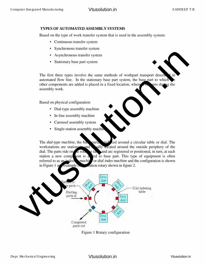
TYPES OF AUTOMATED ASSEMBLY SYSTEMS
Based on the type of work transfer system that is used in the assembly system:
• Continuous transfer system
• Synchronous transfer system
• Asynchronous transfer system
• Stationary base part system
The first three types involve the same methods of workpart transport described in
automated flow line. In the stationary base part system, the base part to which the
other components are added is placed in a fixed location, where it remains during the
assembly work.
Based on physical configuration:
• Dial-type assembly machine
• In-line assembly machine
• Carousel assembly system
• Single-station assembly machine
The dial-type machine, the base partare indexed around a circular table or dial. The
workstations are stationary and usually located around the outside periphery of the
dial. The parts ride on the rotating table and arc registered or positioned, in turn, at each
station a new component is added to base part. This type of equipment is often
referred to as an indexing machine or dial index machine and the configuration is shown
in Figure 1 and example of six station rotary shown in figure 2.
Figure 1 Rotary configuration
Computer Integrated Manufacturing SANDEEP T R
Dept. Mechanical Engineering Vtusolution.in
Vtusolution.in
Vtusolution.in
vtuso
lution
.in
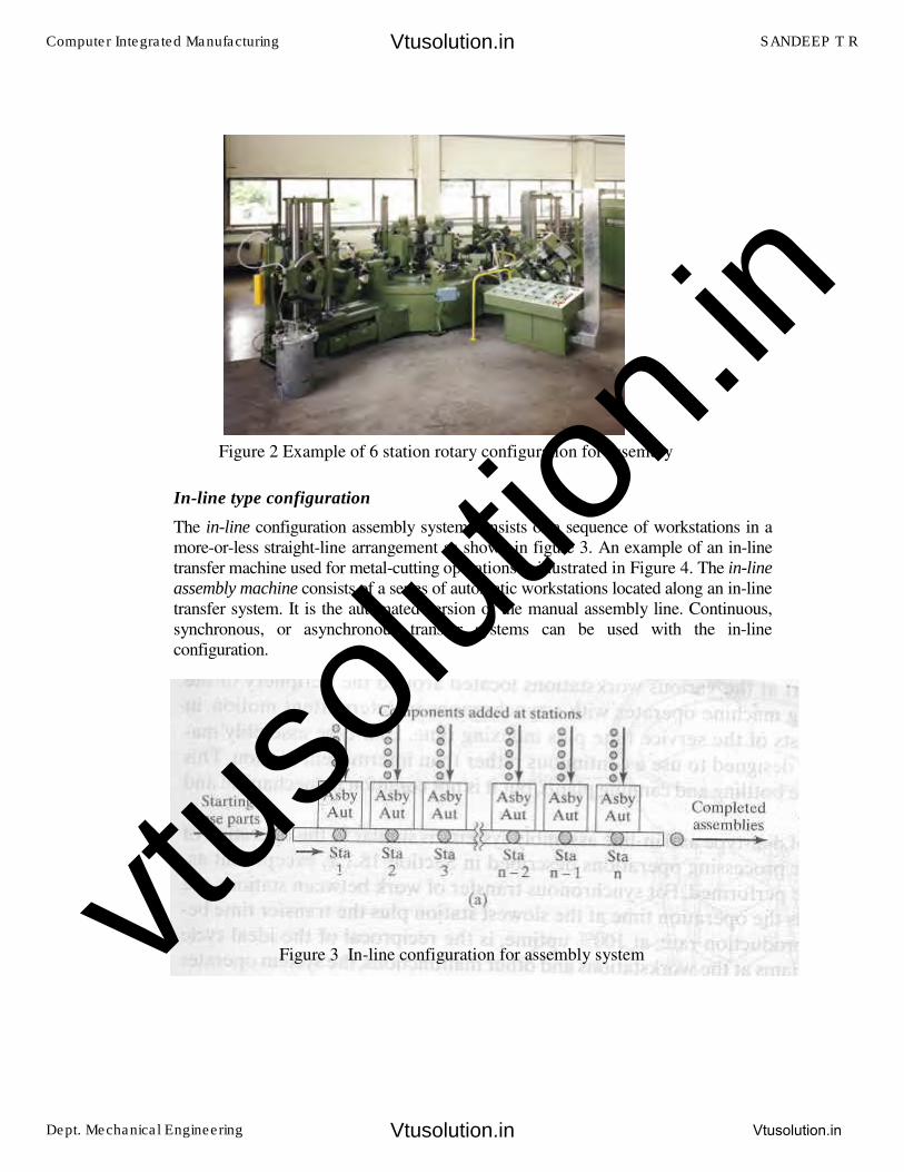
In-line type configuration
The in-line configuration assembly system consists of a sequence of workstations in a
more-or-less straight-line arrangement as shown in figure 3. An example of an in-line
transfer machine used for metal-cutting operations is illustrated in Figure 4. The in-line
assembly machine consists of a series of automatic workstations located along an in-line
transfer system. It is the automated version of the manual assembly line. Continuous,
synchronous, or asynchronous transfer systems can be used with the in-line
configuration.
Figure 2 Example of 6 station rotary configuration for assembly
Figure 3 In-line configuration for assembly system
Computer Integrated Manufacturing SANDEEP T R
Dept. Mechanical Engineering Vtusolution.in
Vtusolution.in
Vtusolution.in
vtuso
lution
.in
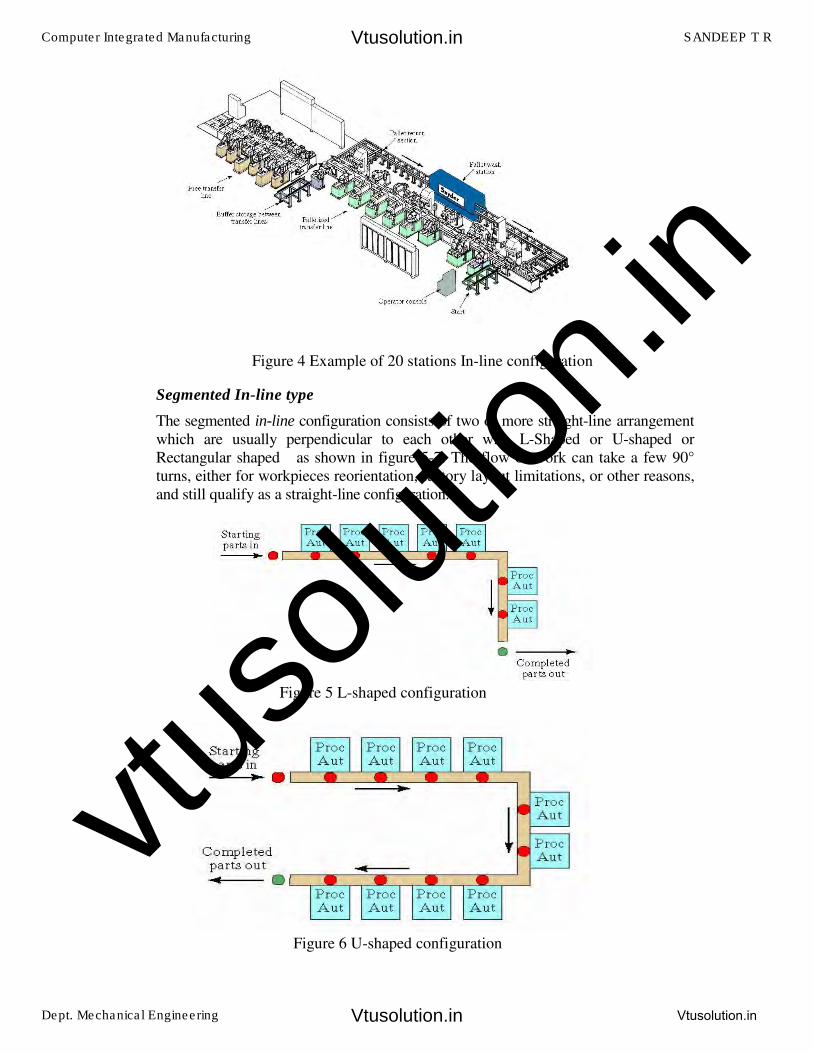
Segmented In-line type
The segmented in-line configuration consists of two or more straight-line arrangement
which are usually perpendicular to each other with L-Shaped or U-shaped or
Rectangular shaped as shown in figure 5-7. The flow of work can take a few 90°
turns, either for workpieces reorientation, factory layout limitations, or other reasons,
and still qualify as a straight-line configuration.
Figure 5 L-shaped configuration
Figure 6 U-shaped configuration
Figure 4 Example of 20 stations In-line configuration
Computer Integrated Manufacturing SANDEEP T R
Dept. Mechanical Engineering Vtusolution.in
Vtusolution.in
Vtusolution.in
vtuso
lution
.in
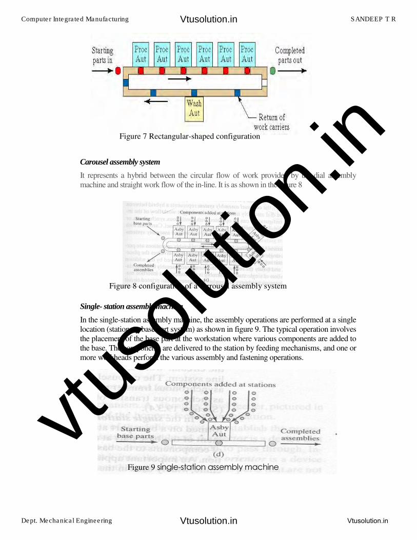
Carousel assembly system
It represents a hybrid between the circular flow of work provided by the dial assembly
machine and straight work flow of the in-line. It is as shown in the figure 8
Single- station assembly machine
In the single-station assembly machine, the assembly operations are performed at a single
location (stationary base part system) as shown in figure 9. The typical operation involves
the placement of the base part at the workstation where various components are added to
the base. The components are delivered to the station by feeding mechanisms, and one or
more workheads perform the various assembly and fastening operations.
Figure 7 Rectangular-shaped configuration
Figure 8 configuration of a carrousel assembly system
Figure 9 ����������������� ���������
Computer Integrated Manufacturing SANDEEP T R
Dept. Mechanical Engineering Vtusolution.in
Vtusolution.in
Vtusolution.in
vtuso
lution
.in

PARTS FEEDING DEVICES
In each of the configurations described above, a means of delivering the components to
the assembly workhead must be designed. In this section we discuss these devices
and their operation.
Elements of the parts delivery system
The hardware system that delivers components to the workhead in an automated
assembly system typically consists of the following elements as shown in figure 10:
� Hopper: This is the container into which the components are loaded at the
workstation. A separate hopper is used for each component type. The
components are usually loaded into the hopper in bulk. This means that the parts
are randomly oriented initially in the hopper.
� Parts feeder: This is a mechanism that removes the components from the
hopper one at a time for delivery to the assembly workhead. The hopper and parts
feeder are often combined into one operating mechanism. The vibratory bowl
feeder, pictured in Figure 11, is a very common example of the hopper-feeder
combination.
Figure 10 elements of part delivery system
Computer Integrated Manufacturing SANDEEP T R
Dept. Mechanical Engineering Vtusolution.in
Vtusolution.in
Vtusolution.in
vtuso
lution
.in
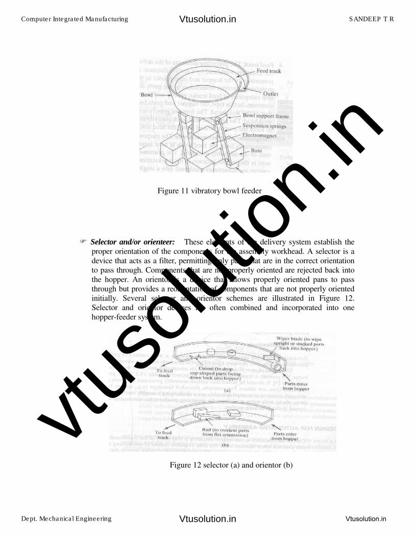
� Selector and/or orienteer: These elements of the delivery system establish the
proper orientation of the components for the assembly workhead. A selector is a
device that acts as a filter, permitting only parts that are in the correct orientation
to pass through. Components that are not properly oriented are rejected back into
the hopper. An orientor is a device that allows properly oriented pans to pass
through but provides a reorientation of components that are not properly oriented
initially. Several selector and orientor schemes are illustrated in Figure 12.
Selector and orientor devices are often combined and incorporated into one
hopper-feeder system.
Figure 11 vibratory bowl feeder
Figure 12 selector (a) and orientor (b)
Computer Integrated Manufacturing SANDEEP T R
Dept. Mechanical Engineering Vtusolution.in
Vtusolution.in
Vtusolution.in
vtuso
lution
.in
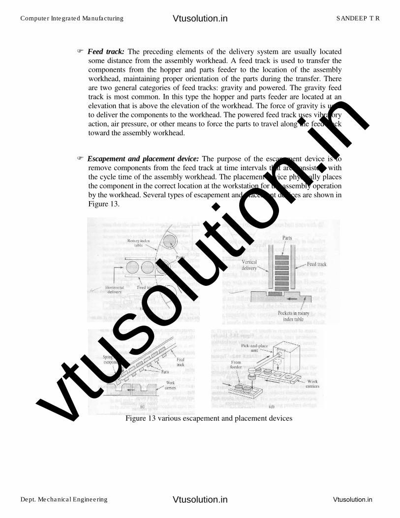
� Feed track: The preceding elements of the delivery system are usually located
some distance from the assembly workhead. A feed track is used to transfer the
components from the hopper and parts feeder to the location of the assembly
workhead, maintaining proper orientation of the parts during the transfer. There
are two general categories of feed tracks: gravity and powered. The gravity feed
track is most common. In this type the hopper and parts feeder are located at an
elevation that is above the elevation of the workhead. The force of gravity is used
to deliver the components to the workhead. The powered feed track uses vibratory
action, air pressure, or other means to force the parts to travel along the feed track
toward the assembly workhead.
� Escapement and placement device: The purpose of the escapement device is to
remove components from the feed track at time intervals that are consistent with
the cycle time of the assembly workhead. The placement device physically places
the component in the correct location at the workstation for the assembly operation
by the workhead. Several types of escapement and placement devices are shown in
Figure 13.
Figure 13 various escapement and placement devices
Computer Integrated Manufacturing SANDEEP T R
Dept. Mechanical Engineering Vtusolution.in
Vtusolution.in
Vtusolution.in
vtuso
lution
.in
Quantitative analysis of the delivery system operation
The parts feeding mechanism is capable of removing parts from the hopper at a certain
rate f . These parts are assumed to be in random orientation initially, and must be
presented to the selector or orientor to establish the correct orientation. In the case of
the selector, a certain proportion of the parts will be correctly oriented initially and
these will be allowed to pass through. The remaining proportion, which is incorrectly
oriented, will be rejected back into the hopper. In the case of the orientor, the parts
that are incorrectly oriented will be reoriented, resulting ideally in a 100% rate of parts
passing through the orientor device. In many delivery system designs, the functions of
the selector and the orientor will be combined. Let us define θ to be the proportion of
components that pass through the setector-orientor process and are correctly oriented
for delivery into the feed track. Hence the effective rate of delivery of components
from the hopper into the feed track will be fθ . The remaining proportion, (1- fθ ),
will be recirculated back into the hopper.
Assuming that the delivery rate of components fθ is greater than the cycle rate Rc of
the assembly machine, a means of limiting the size of the queue in the feed track must
be established. This is generally accomplished by placing a sensor (e.g., limit switch,
optical sensor, etc.) near the top of the feed track, which is used to turn off the feeding
mechanism when the feed track is full. This sensor is referred to as the high-level
sensor, and its location defines the active length Lf2 of the feed track. If the length of a
component in the feed track is Lc, the number of parts that can be held in the feed track is
nf2 = Lf2/Lc. The length of the components must be measured from a point on a given
component to the corresponding point on the next component in the queue to allow for
possible overlap of parts. The value of nf2 is the capacity of the feed track.
Another sensor is placed along the feed track at some distance from the first sensor and
is used to restart the feeding mechanism-again. Defining the location of this low-
level sensor as Lfl, the number of components in the feed track at this point is nf1 =
Lf1/Lc.
The rate at which the quantity of parts in the buffer will be reduced when the high-level
sensor is actuated = Rc, where Re is the theoretical cycle rate of the assembly
machine. On average, the rate at which the quantity of parts will increase upon
actuation of the low-level sensor is fθ - RC However, the rate of increase will
not be uniform due lo the random nature of the feeder-selector operation.
Computer Integrated Manufacturing SANDEEP T R
Dept. Mechanical Engineering Vtusolution.in
Vtusolution.in
Vtusolution.in
vtuso
lution
.in
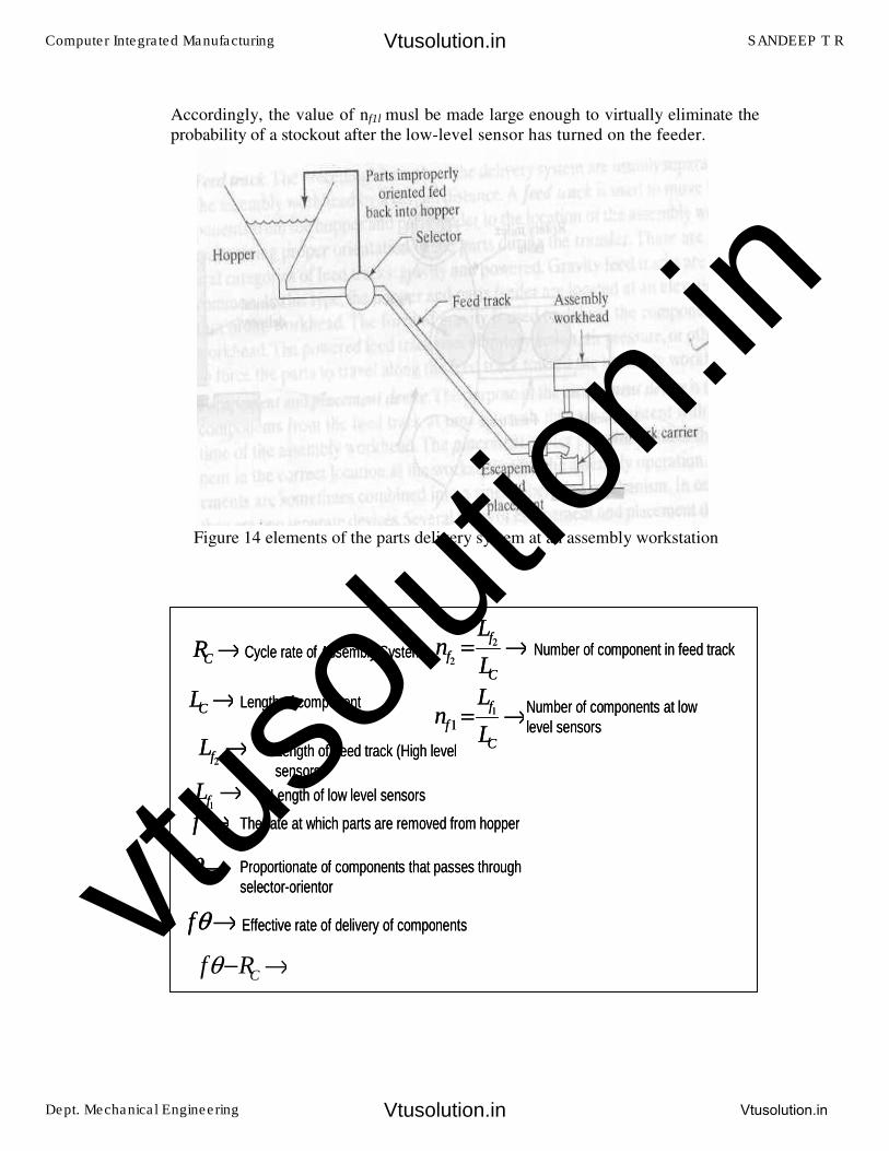
Accordingly, the value of nf1l musl be made large enough to virtually eliminate the
probability of a stockout after the low-level sensor has turned on the feeder.
ANALYSIS OF MULTISTATION ASSEMBLY MACHINES
Figure 14 elements of the parts delivery system at an assembly workstation
f → The rate at which parts are removed from hopperf → The rate at which parts are removed from hopper
θ → Proportionate of components that passes throughselector-orientor
θ → Proportionate of components that passes throughselector-orientor
Cf Rθ− →
CR → Cycle rate of Assembly SystemCR → Cycle rate of Assembly System
CL → Length of componentCL → Length of component
2
2
f
f
C
Ln
L= → Number of component in feed track
2
2
f
f
C
Ln
L= → Number of component in feed track
1
1
f
f
C
Ln
L= →
Number of components at lowlevel sensors
1
1
f
f
C
Ln
L= →
Number of components at lowlevel sensors
2fL → Length of feed track (High level
sensors2f
L → Length of feed track (High levelsensors
1fL → Length of low level sensors
1fL → Length of low level sensors
Effective rate of delivery of componentsfθ → Effective rate of delivery of componentsfθ →
Computer Integrated Manufacturing SANDEEP T R
Dept. Mechanical Engineering Vtusolution.in
Vtusolution.in
Vtusolution.in
vtuso
lution
.in
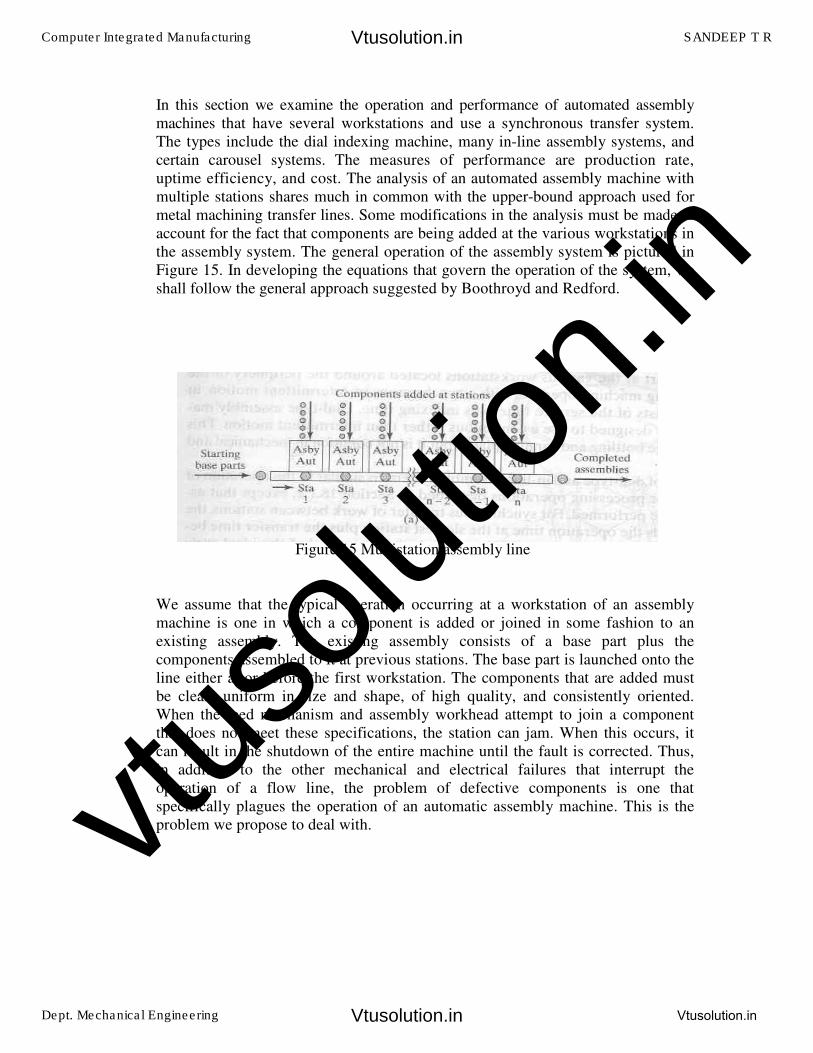
In this section we examine the operation and performance of automated assembly
machines that have several workstations and use a synchronous transfer system.
The types include the dial indexing machine, many in-line assembly systems, and
certain carousel systems. The measures of performance are production rate,
uptime efficiency, and cost. The analysis of an automated assembly machine with
multiple stations shares much in common with the upper-bound approach used for
metal machining transfer lines. Some modifications in the analysis must be made to
account for the fact that components are being added at the various workstations in
the assembly system. The general operation of the assembly system is pictured in
Figure 15. In developing the equations that govern the operation of the system, we
shall follow the general approach suggested by Boothroyd and Redford.
We assume that the typical operation occurring at a workstation of an assembly
machine is one in which a component is added or joined in some fashion to an
existing assembly. The existing assembly consists of a base part plus the
components assembled to it at previous stations. The base part is launched onto the
line either at or before the first workstation. The components that are added must
be clean, uniform in size and shape, of high quality, and consistently oriented.
When the feed mechanism and assembly workhead attempt to join a component
that does not meet these specifications, the station can jam. When this occurs, it
can result in the shutdown of the entire machine until the fault is corrected. Thus,
in addition to the other mechanical and electrical failures that interrupt the
operation of a flow line, the problem of defective components is one that
specifically plagues the operation of an automatic assembly machine. This is the
problem we propose to deal with.
Figure 15 Multistation assembly line
Computer Integrated Manufacturing SANDEEP T R
Dept. Mechanical Engineering Vtusolution.in
Vtusolution.in
Vtusolution.in
vtuso
lution
.in
The assembly machine as a game of chance
Defective parts are a fact of manufacturing life. Defects occur with a certain
fraction defective rate, q. In the operation of an assembly workstation, q can be
considered as the probability that the next component is defective. When an
attempt is made to feed and assemble a defective component, the defect might or
might not cause the station to jam. Let m equal the probability that a defect will
result in the malfunction and stoppage of the workstation. Since the values of q and
m may be different for different stations, we subscript these terms as qi and mi,
where i — 1, 2, ...n the number of stations on the assembly machine.
Considering what happens at a particular workstation, station i, there are three
possible events that might occur when the feed mechanism attempts to feed the
component and the assembly device attempts to join it to the existing assembly:
1. The component is defective and causes a station jam,
2. The component is defective but does not cause a station jam.
3. The component is not defective.
The probability of the first event is the product of the fraction defective rate for the
station, qi, multiplied by the probability that a defect will cause the station to stop,
mi,. the probability that a part will jam at station i. For an assembly machine,
The second possible event, when the component is defective but does not cause a
station jam, has a probability given by
With this outcome, a bad part is joined to the existing assembly, perhaps rendering
the entire assembly defective.
The third possibility is obviously the most desirable. The probability that the com-
ponent is not defective is equal to the proportion of good parts
i i iP m q=
( )1i i i
P m q= −
( )1i iP q= −
Computer Integrated Manufacturing SANDEEP T R
Dept. Mechanical Engineering Vtusolution.in
Vtusolution.in
Vtusolution.in
vtuso
lution
.in
The probabilities of the three possible events must sum to unity.
To determine the complete distribution of possible outcomes that can occur on an n-
station assembly machine, we can multiply the terms of above Equation together
for all stations:
In the special case of Eq., where all are equal and all are equal, then equation
becomes
Measures of performance
Fortunately, we are not required to calculate every term to make use of the concept
of assembly machine operation provided by above Equations. One of the
characteristics of performance that we might want to know is the proportion of
assemblies that contain one or more defective components. Two of the three terms
in above Equation represent events that result in the addition of good components
at a given station. The first term is i im q . which indicates a line stop but also
means that a defective component has not been added to the assembly. The other
term is ( )1 iq− , which means that a good component has been added at the station.
The sum of these two terms represents the probability that a defective component
will not be added at station i. Multiplying these probabilities for all stations, we
get the proportion of acceptable product coming off the line, ap
P
( )1
1n
ap i i i
i
P m q q=
= + −� �� �∏
In the special case where all are equal and all i
Q are equal, then equation
becomes
( ) ( )1 1 1i i i i i
m q m q q+ − + − =
im
( ) ( )1
1 1 1n
i i i i i
i
m q m q q=
+ − + − =� �� �∏
iq
( ) ( )1 1 1n
m q m q q+ − + − =� �� �
im
( )1n
ap i i iP m q q= + −� �� �
Computer Integrated Manufacturing SANDEEP T R
Dept. Mechanical Engineering Vtusolution.in
Vtusolution.in
Vtusolution.in
vtuso
lution
.in
If this is the proportion of assemblies with no defective components, the proportion
of assemblies that contain at least one defect is given by
In the special case where all i
m are equal and all i
Q are equal, then equation
becomes
,
In addition to the proportions of good and bad assemblies as measures of perfor-
mance for an assembly machine, we are also interested in the machine's production
rate, proportions of uptime and downtime, and average cost per unit produced.
To calculate production rate we must first determine the frequency of downtime
occurrences per cycle, f. If each station jam results in a machine downtime
occurrence, f can be found by taking the expected number of station jams per cycle.
In the special case where all i
m are equal and all i
Q are equal, then equation
becomes
Average production time per assembly is therefore given by
Tc = ideal cycle time
Td = average downtime per occurrence
In the special case where all i
m are equal and all i
Q are equal, then equation
becomes
( )1
1 1n
qp i i i
i
P m q q=
= − + −� �� �∏
( )1 1n
qp i i iP m q q= − + −� �� �
1 1
n n
i i i
i i
F P m q= =
= =� �
F nm q=
1
n
P C i i D
i
T T m q T=
= +�
P C DT T nm q T= +
Computer Integrated Manufacturing SANDEEP T R
Dept. Mechanical Engineering Vtusolution.in
Vtusolution.in
Vtusolution.in
vtuso
lution
.in
The rate of production of acceptable product is given by equation
In the special case where all i
m are equal and all i
Q are equal, then equation
becomes
The line efficiency is calculated as the ratio of ideal cycle time to average production
time.
The proportion of downtime, D, is the average downtime per cycle divided by the
average production time is given by
The cost per assembly produced, is given by
1P
P
RT
=
( )1
1n
i i iapi
ap
P p
m q qP
RT T
=
+ −� �� �= =
∏
( )( )1n
ap
P
mq qR
T
+ −=
C C
P C D
T TE
T T nm q T= =
+
D D
P C D
nm q T nm q TD
T T nm q T= =
+
( )( )1
m L P t m L P t
pc n
ap
C C T C C C T CC
Pmq q
+ × + + × += =
+ −
Computer Integrated Manufacturing SANDEEP T R
Dept. Mechanical Engineering Vtusolution.in
Vtusolution.in
Vtusolution.in
vtuso
lution
.in
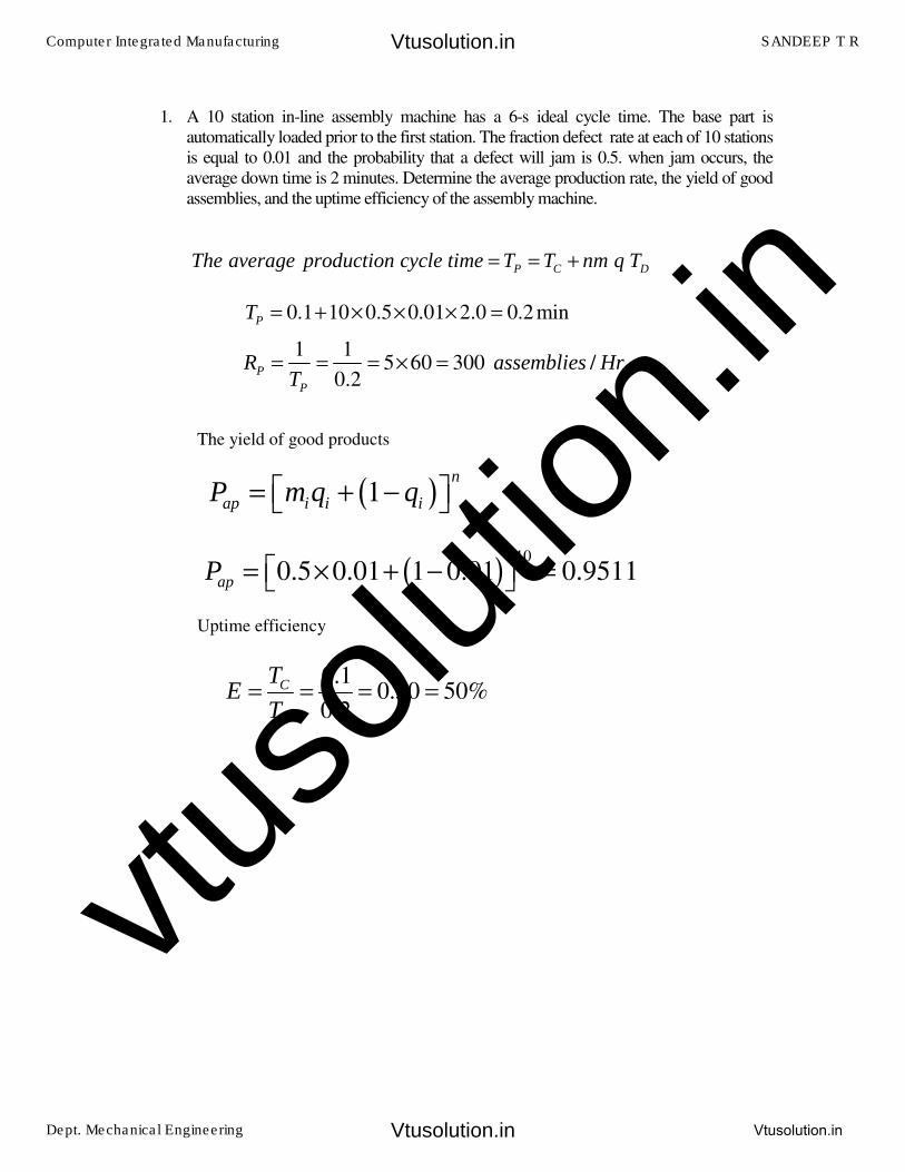
1. A 10 station in-line assembly machine has a 6-s ideal cycle time. The base part is
automatically loaded prior to the first station. The fraction defect rate at each of 10 stations
is equal to 0.01 and the probability that a defect will jam is 0.5. when jam occurs, the
average down time is 2 minutes. Determine the average production rate, the yield of good
assemblies, and the uptime efficiency of the assembly machine.
P C DThe average production cycle time T T nm q T= = +
0.1 10 0.5 0.01 2.0 0.2 minP
T = + × × × =
1 15 60 300 /
0.2P
P
R assemblies HrT
= = = × =
( )1n
ap i i iP m q q= + −� �� �
( )10
0.5 0.01 1 0.01 0.9511apP = × + − =� �� �
The yield of good products
0.10.50 50%
0.2
C
P
TE
T= = = =
Uptime efficiency
Computer Integrated Manufacturing SANDEEP T R
Dept. Mechanical Engineering Vtusolution.in
Vtusolution.in
Vtusolution.in
vtuso
lution
.in

7.5 ANALYSIS OF A SINGLE-STATION ASSEMBLY MACHINE
The single-station assembly machine can be pictured as shown in Figure 16. We
assume a single workhead, with several components feeding into the station to be
assembled. Let us use n to represent the number of distinct assembly elements that
are performed on the machine. Each element has an element time, Tei, where i =
1,2,..., n. The ideal cycle time for the single-station assembly machine is the sum of
the individual element times of the assembly operations to be performed on the
machine, plus the handling time to load the base part into position and unload the
completed assembly. We can express this ideal cycle time as
where Th is the handling time,
Many of the assembly elements involve the addition of a component to the existing
subassembly. As in our analysis of the multiple-station assembly system, each
component type has a certain fraction defect rate, qi and there is a certain probability
that a defective component will jam the workstation, mi When a jam occurs, the
assembly machine stops, and it takes an average Td to clear the jam and restart the
system. The inclusion of downtime resulting from jams in the machine cycle time
gives.
Average production time per assembly is therefore given by
Figure 16 Single station assembly machine
1
n
C h e i
i
T T T=
= + �
1
n
P C i i D
i
T T m q T=
= +�
Computer Integrated Manufacturing SANDEEP T R
Dept. Mechanical Engineering Vtusolution.in
Vtusolution.in
Vtusolution.in
vtuso
lution
.in
Tc = ideal cycle time
Td = average downtime per occurrence
In the special case where all i
m are equal and all i
Q are equal, then equation
becomes
The rate of production of acceptable product is given by equation
In the special case where all i
m are equal and all i
Q are equal, then equation
becomes
The line efficiency is calculated as the ratio of ideal cycle time to average production
time.
The proportion of downtime, D, is the average downtime per cycle divided by the
average production time is given by
The cost per assembly produced, is given by
P C DT T nm q T= +
1P
P
RT
=
( )1
1n
i i iapi
ap
P p
m q qP
RT T
=
+ −� �� �= =
∏
( )( )1n
ap
P
mq qR
T
+ −=
C C
P C D
T TE
T T nm q T= =
+
D D
P C D
nm q T nm q TD
T T nm q T= =
+
( )( )1
m L P t m L P t
pc n
ap
C C T C C C T CC
Pmq q
+ × + + × += =
+ −
Computer Integrated Manufacturing SANDEEP T R
Dept. Mechanical Engineering Vtusolution.in
Vtusolution.in
Vtusolution.in
vtuso
lution
.in
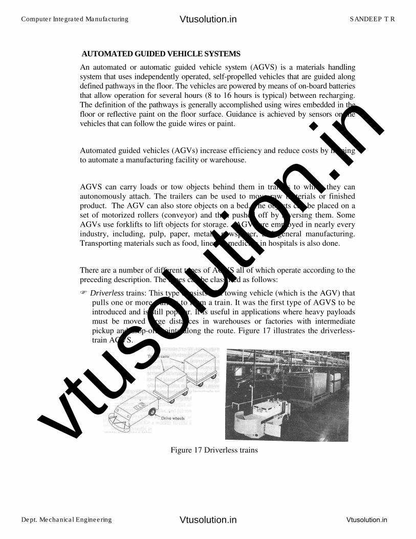
AUTOMATED GUIDED VEHICLE SYSTEMS
An automated or automatic guided vehicle system (AGVS) is a materials handling
system that uses independently operated, self-propelled vehicles that are guided along
defined pathways in the floor. The vehicles are powered by means of on-board batteries
that allow operation for several hours (8 to 16 hours is typical) between recharging.
The definition of the pathways is generally accomplished using wires embedded in the
floor or reflective paint on the floor surface. Guidance is achieved by sensors on the
vehicles that can follow the guide wires or paint.
Automated guided vehicles (AGVs) increase efficiency and reduce costs by helping
to automate a manufacturing facility or warehouse.
AGVS can carry loads or tow objects behind them in trailers to which they can
autonomously attach. The trailers can be used to move raw materials or finished
product. The AGV can also store objects on a bed. The objects can be placed on a
set of motorized rollers (conveyor) and then pushed off by reversing them. Some
AGVs use forklifts to lift objects for storage. AGVs are employed in nearly every
industry, including, pulp, paper, metals, newspaper, and general manufacturing.
Transporting materials such as food, linen or medicine in hospitals is also done.
There are a number of different types of AGVS all of which operate according to the
preceding description. The types can be classified as follows:
� Driverless trains: This type consists of a towing vehicle (which is the AGV) that
pulls one or more trailers to form a train. It was the first type of AGVS to be
introduced and is still popular. It is useful in applications where heavy payloads
must be moved large distances in warehouses or factories with intermediate
pickup and drop-off points along the route. Figure 17 illustrates the driverless-
train AGVS.
Figure 17 Driverless trains
Computer Integrated Manufacturing SANDEEP T R
Dept. Mechanical Engineering Vtusolution.in
Vtusolution.in
Vtusolution.in
vtuso
lution
.in
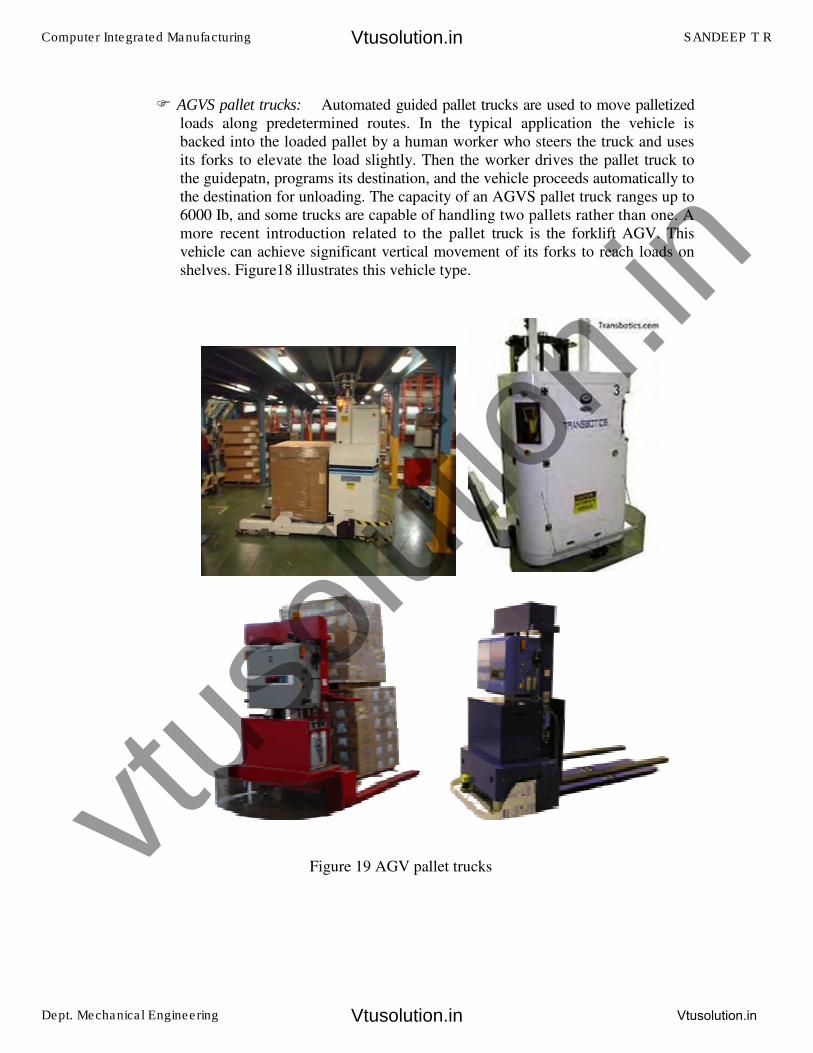
� AGVS pallet trucks: Automated guided pallet trucks are used to move palletized
loads along predetermined routes. In the typical application the vehicle is
backed into the loaded pallet by a human worker who steers the truck and uses
its forks to elevate the load slightly. Then the worker drives the pallet truck to
the guidepatn, programs its destination, and the vehicle proceeds automatically to
the destination for unloading. The capacity of an AGVS pallet truck ranges up to
6000 Ib, and some trucks are capable of handling two pallets rather than one. A
more recent introduction related to the pallet truck is the forklift AGV. This
vehicle can achieve significant vertical movement of its forks to reach loads on
shelves. Figure18 illustrates this vehicle type.
Figure 19 AGV pallet trucks
Computer Integrated Manufacturing SANDEEP T R
Dept. Mechanical Engineering Vtusolution.in
Vtusolution.in
Vtusolution.in
vtuso
lution
.in
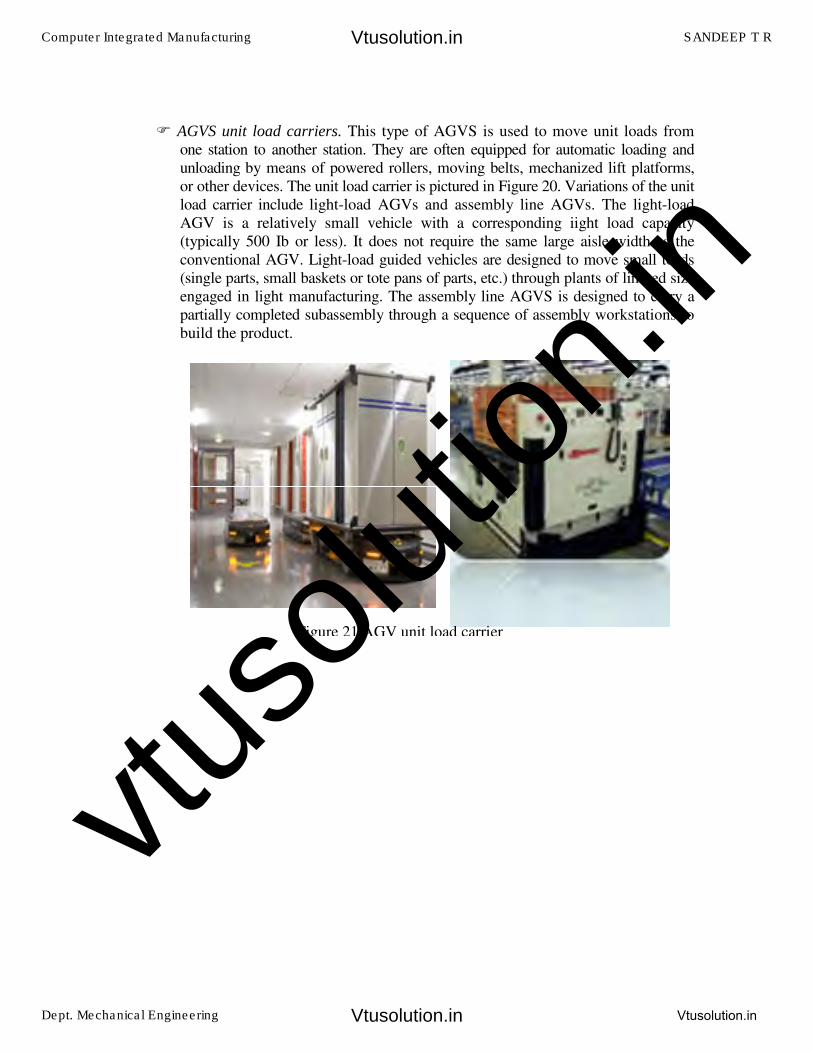
� AGVS unit load carriers. This type of AGVS is used to move unit loads from
one station to another station. They are often equipped for automatic loading and
unloading by means of powered rollers, moving belts, mechanized lift platforms,
or other devices. The unit load carrier is pictured in Figure 20. Variations of the unit
load carrier include light-load AGVs and assembly line AGVs. The light-load
AGV is a relatively small vehicle with a corresponding iight load capacity
(typically 500 Ib or less). It does not require the same large aisle width as the
conventional AGV. Light-load guided vehicles are designed to move small toads
(single parts, small baskets or tote pans of parts, etc.) through plants of limited size
engaged in light manufacturing. The assembly line AGVS is designed to carry a
partially completed subassembly through a sequence of assembly workstations to
build the product.
Figure 21 AGV unit load carrier
Computer Integrated Manufacturing SANDEEP T R
Dept. Mechanical Engineering Vtusolution.in
Vtusolution.in
Vtusolution.in
vtuso
lution
.in
Vehicle guidance and routing
There are several functions that must be performed to operate any automated
guided vehicle system successfully. These functions are:
1, Vehicle guidance and routing
2, Traffic control and safety
3, System management
We describe these functions in this and the following two subsections.
The term guidance system refers to the method by which the AGVS pathways are
defined and the vehicle control systems that follow the pathways. As indicated above,
there are two principal methods currently in use lo define the pathways along the floor:
embedded guide wires and paint strips. Of the two types, the guide wire system is
the more common in warehouse and factory applications.
In the guide wire method the wires are usually embedded in a small channel cut into
the surface of the floor. The channel is typically about 1/8 in. wide and 1/2 in. deep.
After the guide wires are installed, the channel slot is filled so as to eliminate the
discontinuity in the floor surface as shown in figure 22. An alternative but less
permanent way to install the guide wires is to tape them to the floor. A frequency
generator provides the guidance signal carried in the wire. The signal is of relatively
low voltage (less than 40 V), low current (less than 400 mA), and has a frequency in
the range 1 to 15 kHz. This signal level creates a magnetic field along the pathway
that is followed by sensors on-board each vehicle. The operation of a typical system is
illustrated in Figure 22 Two sensors (coils) are mounted on the vehicle on either side of
the guide wire. When the vehicle is moving along a course such that the guide wire is
directly between the two coils, the intensity of the magnetic field measured by each
coil will be equal. If the vehicle strays to one side or the other, or if the guide wire
path curves, the magnetic field intensity at the two sensors will be different. This
difference is used to control the steering motor, which makes the required changes in
vehicle direction to equalize the two sensor signals, thereby tracking the defined
pathway.
Computer Integrated Manufacturing SANDEEP T R
Dept. Mechanical Engineering Vtusolution.in
Vtusolution.in
Vtusolution.in
vtuso
lution
.in

When paint strips are used to define the vehicle pathways, the vehicle possesses an
optical sensor system that is capable of tracking the paint. The strips can be taped,
sprayed, or painted on the floor. One system uses a l-in.-wide paint strip containing
fluorescent particles that reflect an ultraviolet (UV) light source on the vehicle. An on-
board sensor detects the reflected light in the strip and controls the steering
mechanism to follow it. The paint guidance system is useful in environments where
electrical noise would render the guide wire system unreliable or when the installation
of guide wires in the floor surface would not be appropriate. One problem with the
paint strip guidance method is that the paint strip must be maintained (kept clean and
unscratched).
A safety feature used in the operation of most guidance systems is automatic stopping of
the vehicle in the event that it accidentally strays more than a few inches (typically 2
to 6 in.) from the guide path. This automatic-stopping feature prevents the vehicle
from running wild in the building. Alternatively, in the event that the vehicle is off
the guide path (e.g., for manual loading of a pallet truck), it is capable of locking
onto the guide wire or paint strip if moved within the same few inches of it. The
distance is referred to as the vehicle's acquisition distance.
The use of microprocessor controls on-board the vehicles has led to the development of
a feature called dead reckoning. This term refers to the capability of the vehicle to
travel along a route that does not follow the defined pathway in the floor. The micro-
processor computes the number of wheel rotations and the operation of the steering
motor required to move along the desired path. Dead reckoning might be employed
by the vehicle to cross a steel plate in the factory floor (where guide wires cannot be
Figure 22 wire guided AGV
Computer Integrated Manufacturing SANDEEP T R
Dept. Mechanical Engineering Vtusolution.in
Vtusolution.in
Vtusolution.in
vtuso
lution
.in
installed), or to depart from the guide path for positioning at a load/unload station. At
the completion of the dead-reckoning maneuver, the vehicle is programmed to return
to within (he acquisition distance of the guide path to resume normal guidance
control.
Routing in an AGVS is concerned with the problem of selecting among alternative
pathways available to a vehicle in its travel to a defined destination point in the
system. A typical guided vehicle layout, one that exploits the capabilities of modern
AGVS technology, contains features such as multiple loops, branches, side tracks,
and spurs, in addition to the required pickup and drop-off stations. Vehicles in the
system must decide which path to take to reach a defined destination point.
When a vehicle approaches a branching point in which the guide path splits into two
(or more) directions, a decision must be made as to which path the vehicle should
take. This is sometimes referred to as a decision point for the vehicle. There are two
methods used in commercial AGV systems to permit the vehicle to decide which
path to take:
1. Frequency select method
2. Path switch select method
In the frequency select method, the guide wires leading into the two separate paths at
the branch have different frequencies. As the vehicle enters the decision point, it reads
an identification code on the floor to identify its location. Depending on its
programmed destination, the vehicle selects one of the guide paths by deciding
which frequency to track. This method requires a separate frequency generator for
each frequency that is used in the guide path layout. This usually means that two or
three generators are needed in the system. Additional channels must often be cut into
the floor with the frequency select method to provide for bypass channels where only
the main channel needs to be powered for vehicle tracking.
The path switch select method uses a single frequency throughout the guide path
layout. In order to control the path of a vehicle at a decision point, the power is
switched off in ail branches except the one on which the vehicle is to travel. To
accomplish routing by the path switch select method, the guide path layout most be
divided into blocks that can be independently turned on and off by means of controls
mounted on the floor near their respective blocks. These control units are operated by
the vehicles as they move in the various blocks. As a vehicle enters a decision point, it
activates a floor-mounted switching device connected to the control unit for the
relevant block. The control unit activates the desired guide path and turns off the
alternative branch or branches.
Computer Integrated Manufacturing SANDEEP T R
Dept. Mechanical Engineering Vtusolution.in
Vtusolution.in
Vtusolution.in
vtuso
lution
.in
Traffic control and safety
The purpose of traffic control for an AGVS is to prevent collisions between vehicles
traveling along the same guide path in the layout. This purpose is usually
accomplished by means of a control system called the blocking system. The term
"blocking" suggests that a vehicle traveling along a given guide path is in some way
prevented from hitting any vehicle ahead of it. There are several means used in
commercial AGV systems to accomplish blocking. They are:
1. On-board vehicle sensing
2. Zone blocking
On-board vehicle sensing and zone blocking are often used in combination to
implement a comprehensive blocking system.
On-board vehicle sensing (sometimes called forward sensing) involves the use of
some form of sensor system to detect the presence of vehicles and carts ahead on the
same guide wire. The sensors used on commercial guided vehicles include optical
sensors and ultrasonic systems. When the on-board sensor detects an obstacle (e.g,
another guided vehicle) in front of it, the vehicle stops. When the obstacle is removed,
the vehicle proceeds. Assuming that the sensor system is 100% effective, collisions
between vehicles are avoided and traffic is controlled. Unfortunately, the effectiveness
of forward sensing is limited by the capability of the sensor system to detect vehicles
in front of it on the guide path. Since the sensors themselves are most effective in
detecting obstacles directly ahead of the vehicle, these systems are most appropriate
on layouts that contain long stretches of straight pathways. They are less effective at
turns and convergence points where forward vehicles may not be directly in front of
the sensor.
The concept of zone control is simple. The AGVS layout is divided into separate zones,
and the operating rule is that no vehicle is permitted to enter a zone if that zone is
already occupied by another vehicle. The length of a zone is sufficient to hold one
vehicle (or a train in driverless train systems) plus an allowance for safety and other
considerations. These other considerations include the number of vehicles in the
system, the size and complexity of the layout, and the objective of minimizing the
number of separate zone controls. When one vehicle occupies a given zone, any
trailing vehicle is not allowed into that zone. The leading vehicle must proceed into
the next zone before the trailing vehicle can occupy the given zone.
Computer Integrated Manufacturing SANDEEP T R
Dept. Mechanical Engineering Vtusolution.in
Vtusolution.in
Vtusolution.in
vtuso
lution
.in

By controlling the forward movement of vehicles in the separate zones, collisions are
prevented and traffic in the overall system is controlled. The concept is illustrated in
Figure 23 in its simplest form. More complicated zone control schemes separate any
two vehicles by a blocked zone.
One means of implementing zone control is to use separate control units for each
zone. These controls are mounted along the guide path and are actuated by the
vehicle in the zone. When a vehicle enters a given zone, it activates the block in the
previous (upstream) zone to block any trailing vehicle from moving forward and
colliding with the present vehicle. As the present vehicle moves into the next
(downstream) zone, it activates the block in that zone and deactivates the block in the
previous zone. In effect, zones are turned on and off to control vehicle movement by
the blocking system.
In addition to avoiding collisions between vehicles, a related objective is the safety of
human beings who might be located along the route of the vehicles traveling in the
system. There are several devices that are usually included on an automatic guided
vehicle to achieve this safety objective. One of the safety devices is an obstacle-
detection sensor located at the front of each vehicle. This is often the same on-board
sensor as that used in the blocking system to detect the presence of other vehicles
located in front of the sensor. The sensor can detect not only other vehicles, but also
people and obstacles in the path of the vehicle. These obstacle-detection systems are
usually based on optical, infrared, or ultrasonic sensors. The vehicles are
programmed either to stop when an obstacle is sensed ahead of it, or to slow down.
The reason for slowing down is that the sensed object may be located off to the side of
the vehicle path, or directly ahead of the vehicle beyond a turn in the guide path. In
either of these cases, the vehicle should be permitted to proceed at a slower (safer)
speed until it has passed the object or rounded the turn.
Another safety device included on virtually all commercial AG vehicles is an
emergency bumper. This bumper surrounds the front of the vehicle and protrudes
ahead of it by a distance which can be a foot or more. When the bumper makes
contact with an object, the vehifcle is programmed to brake immediately. Depending on
the speed of the vehicle, its load, and other conditions, the braking distance will vary
Figure 23 zone control
Computer Integrated Manufacturing SANDEEP T R
Dept. Mechanical Engineering Vtusolution.in
Vtusolution.in
Vtusolution.in
vtuso
lution
.in
from several inches to several feet. Most vehicles are programmed to require manual
restarting after an obstacle encounter has occurred with the emergency bumper.
Other safety devices on the vehicles include warning lights (blinking or rotating lights)
and/or warning bells. These devices alert people that the vehicle is present.
Finally, another safety feature that prevents runaway vehicles is the inherent op-
erating characteristic of the guidance system: If the vehicle strays by more than a
few inches from the defined path, the vehicle is programmed to stop.
System management
Managing the operations of an AGVS deals principally with the problem of
dispatching vehicles to the points in the system where they are needed (e.g., to
perform pickups and deliveries) in a timely and efficient manner. The system
management function depends on reliable operation of the other system functions
discussed above (guidance, routing, traffic control). There are a number of methods
used in commercial A.GV systems for dispatching vehicles. These methods are
generally used in combination to maximize responsiveness and effectiveness of the
overall system. The dispatching methods include:
* On-board control panel
* Remote call stations
* Central computer control
Each guided vehicle is equipped with some form of control panel for the purpose
of manual vehicle control, vehicle programming, and other functions. Most
commercial vehicles have the capacity to be dispatched by means of this control
panel to a given station in the AGVS layout. Dispatching with an on-board control
panel represents the lowest level of sophistication among the possible methods. Its
advantage is that it provides the AGVS with flexibility and responsiveness to
changing demands on the handling system. Its disadvantage is that it requires
manual attention.
The use of remote call stations is another method that allows the AGVS to respond
to changing demand patterns in the system. The simplest form of call station is a
press button mounted near the load/unload station. This provides a signal to any
passing vehicle to stop at the station in order to accomplish a load transfer
operation. The vehicle might then be dispatched to the desired location by means
of the on-board control panel.
Computer Integrated Manufacturing SANDEEP T R
Dept. Mechanical Engineering Vtusolution.in
Vtusolution.in
Vtusolution.in
vtuso
lution
.in
More sophisticated call stations consist of control panels mounted near the various
stations along the layout. This method permits a vehicle to be stopped at a given
station, and its next destination to be programmed from the remote call panel. This
represents a more automated approach to the dispatching function and is useful in
AGV systems that are capable of automatic loading and unloading operations.
Both of the call station methods described here involve a human interface with the
AGVS at the load/unload station. It is also possible to automate the call function at
an automatic load/unload station. One example is an automated production
workstation that receives raw materials and sends completed parts by means of the
AGVS. The workstation is interfaced with the AGVS to call for vehicles as needed
to perform the loading and unloading procedures.
In large factory and warehouse systems involving a high level of automation, the
AGVS servicing the factory or warehouse must also be highly automated to
achieve efficient operation of the entire production-storage-handling system. Central
computer control is used to accomplish automatic dispatching of vehicles according to a
preplanned schedule of pickups and deliveries in the layout and/or in response to
calls from the various load/unload stations in the system. In this dispatching method, the
central computer issues commands to the vehicles in the system concerning their
destinations and operations to perform. To accomplish the dispatching function, the
central computer must possess real-time information about the location of each vehicle
in the system so that it can make appropriate decisions concerning which vehicles to
dispatch to what locations. Hence, the vehicles must continually communicate their
whereabouts to the central controller.
There are differences in the way these central computer dispatching systems operate.
One of the differences involves the distribution of the decision-making responsibilities
between the central controller and the individual vehicles. At one extreme, the central
computer makes nearly all the decisions about routing of vehicles and other
functions. The central computer plans out the routes for each vehicle and controls the
operation of the guide path zones and other functions, At the opposite extreme, each
individual vehicle possesses a substantial decision-making capability to make its own
routing selections and to control its own operations. The central computer is still
needed to control the overall scheduling and determine which vehicles should go to the
various demand points in the system. However, the vehicles themselves decide which
routes to take and control their own load transfer operations. Vehicles in this second
category are often referred to as "smart" vehicles.
To accomplish the system management function, it is helpful to monitor the overall
operations of the AGVS by means of some form of graphics display. Even with central
computer control it is still desirable for human managers to be able to see the overall
system operations, in order to monitor its general status and to spot problems (e.g.,
traffic jams, breakdowns, etc.). A CRT color graphics display is often used for these
purposes in modem guided vehicle systems.
Computer Integrated Manufacturing SANDEEP T R
Dept. Mechanical Engineering Vtusolution.in
Vtusolution.in
Vtusolution.in
vtuso
lution
.in
Another useful tool in carrying out the systems management function is a system
performance report for each shift (or other appropriate time period) of AGVS
operation. These periodic reports of system performance provide summary
information about proportion uptime, downtime, number of transactions (deliveries)
made during a shift, and more detailed data about each station and each vehicle in the
system. Hard-copy reports containing this type of information permit the system
managers to compare operations from shift to shift and month to month to maintain a
high level of overall system performance.
Applications
Automated Guided Vehicles can be used in a wide variety of applications to transport
many different types of material including pallets, rolls, racks, carts, and containers.
AGVs excel in applications with the following characteristics:
• Repetitive movement of materials over a distance
• Regular delivery of stable loads
• Medium throughput/volume
• When on-time delivery is critical and late deliveries are causing inefficiency
• Operations with at least two shifts
• Processes where tracking material is important
Driverless train operations
Storage/distribution
Assembly line operations
FMS
Mail delivery in offices
Hospitals
Raw Material Handling
Work-in-Process Movement
Pallet Handling
Finished Product Handling
Trailer Loading
Roll Handling
Computer Integrated Manufacturing SANDEEP T R
Dept. Mechanical Engineering Vtusolution.in
Vtusolution.in
Vtusolution.in
vtuso
lution
.in
Battery Charging
1. Driverless train operations: These applications involve the movement of large
quantities of materials over relatively large distances. For example, the moves
are with in a large warehouse or factory building, or between buildings in a
large storage depot. For the movement of trains consisting of 5 to 10 trailers,
this becomes an efficient handling method,
2. Storage/distribution systems: Unit load carriers and pallet trucks are typically
used in these applications. These storage and distribution operations involve the
movement of materials in unit loads (sometimes individual items are moved)
from or to specific locations. The applications often interface the AGVS with
some other automated handling or storage system, such as an automated
storage/retrieval system (AS/RS) in a distribution center. The AGVS delivers
incoming items or unit loads (contained on pallets) from the receiving dock to
the AS/RS, which places the items in storage, and the AS/RS retrieves
individual pallet loads or items from storage and transfers them to vehicles
for delivery to the shipping dock. When the rates of incoming loads and the
outgoing loads are in balance, this mode of -operation permits loads to be
carried in both directions by the AGVS vehicles, thereby increasing the
handling system efficiency.
This type of storage/distribution operation can also be applied in light
manufacturing and assembly operations in which work-in-progress is stored in
a central storage area and distributed to individual workstations for assembly
or processing. Electronics assembly is an example of these types of
applications. Components are "kitted" at the storage area and delivered in tote
pans or trays by the guided vehicles to the assembly workstations in the
plant. Light-load AGV systems are used in these applications.
3. Assembly-line operations: AGV systems are being used in a growing number
of assembly-line applications, based on a trend that began in Europe. In these
applications, the production rate is relatively low (perhaps 4 to 10 min per
station in the line) and there are a variety of different models made on the
production line. 'Between the work stations, components are kitted and
placed on the vehicle for the assembly operations that are to be performed
on the partially completed product at the next station. The workstations are
generally arranged in parallel configurations to add to the flexibility of the
line. Unit load carriers and light-load guided vehicles are the type of AGVS
used in these assembly lines.
4. Flexible manufacturing systems: Another growing application of AGVS
technology is in flexible manufacturing systems (FMS). In this application, the
guided vehicles are used as the materials handling system in the FMS. The
Computer Integrated Manufacturing SANDEEP T R
Dept. Mechanical Engineering Vtusolution.in
Vtusolution.in
Vtusolution.in
vtuso
lution
.in
vehicles deliver work from the staging area (where work is placed on pallet
fixtures, usually manually) to the individual workstations in the system. The
vehicles also move work between stations in the manufacturing system. At a
workstation, the work is transferred from the vehicle platform into the work
area of the station (usually, the table of a machine tool) for processing. At the
completion of processing by that station a vehicle returns to pick up the
work and transport it to the next area. AGV systems provide a versatile
material handling system to complement the flexibility of the FMS operation.
5. Miscellaneous applications: Other applications of automated guided vehicle
systems include non manufacturing and non warehousing applications, such as
mail delivery in office buildings and hospital material handling operations.
Hospital guided vehicles transport meal trays, linen, medical and laboratory
supplies, and other materials between various departments in the building.
These applications typically require movement of the vehicles between
different floors of the hospital, and hospital AGV systems have the capability
to summon and use elevators for this purpose.
Computer Integrated Manufacturing SANDEEP T R
Dept. Mechanical Engineering Vtusolution.in
Vtusolution.in
Vtusolution.in
vtuso
lution
.in
UNIT 6:
COMPUTERIZED MANUFACTURING PLANNING SYSTEM:
Traditional Process Planning:
There are variations in the level of detail found in route sheets among different companies & industries. In the one extreme, process planning is accomplished by releasing the part print to the production shop with the instructions “make to drawing.” Most firms provide a more detailed list of steps describing each operation and identifying each work center. In any case, it is traditionally the task of the manufacturing engineers or industrial engineers in an organization to write these process plans for new part designs to be produced by the shop. The process planning procedure is very much dependent on the experience and judgement of the planner. It is the manufacturing engineer’s responsibility to determine an optimal routing for each new part design. However, the individual engineers each have their own opinions about what constitutes the best routing. Accordingly, there are differences among the operation sequences developed by various planners. We can illustrate rather dramatically these differences by means of an example.
In one case, a total of 42 different routings were developed for various sizes of a relatively simple part called an “expander sleeve.” There were a total of 64 different sizes & styles, each with its own part number. The 42 routings included 20 different machine tools in the shop. The reason for this absence of process standardization was that many different individuals had worked on the parts: 8 or 9 manufacturing engineers, 2 planners and 25 NC part programmers. Upon analysis, it was determined that only two different routings through 4 machines were needed to process the 64 part numbers. It is clear that there were potentially great differences in the perceptions among process planners as to what constitutes the “optimal” method of production.
In addition to this problem of variability among planners, there are often difficulties in the conventional process planning procedure. New machine tools in the factory render old routings less than optimal. Machine breakdowns force shop personnel to use temporary routings, & these become the documented routings even after the machine is repaired. For these reasons and others, a significant proportion of the total number of process plans used in manufacturing are not optimal.
Automated Process Planning:
Because of the problems encountered with manual process planning, attempts have been made in recent years to capture the logic, judgement, and experience required for this important function and incorporate them into computer programs. Based on the characteristics of a given part, the program automatically generates the manufacturing operation sequence. A computer-aided process planning (CAPP) system offers the potential for reducing the routine clerical work of manufacturing engineers. At the same time, it provides the opportunity to generate production routings which are rational, consistent, and perhaps even optimal. Two alternative approaches to computer-aided process planning have been developed. These are:
1. Retrieval-type CAPP systems (also called variant systems)
2. Generative CAPP systems
The two types are described as below:
Computer Integrated Manufacturing SANDEEP T R
Dept. Mechanical Engineering Vtusolution.in
Vtusolution.in
Vtusolution.in
vtuso
lution
.in
Retrieval-type Process Planning systems:
Retrieval-type CAPP systems use parts classification & coding & group technology as a foundation. In this approach, the parts produced in the plant are grouped into part families, distinguished according to their manufacturing characteristics. For each part family, a standard process plan is established. The standard process plan is stored in computer files & then retrieved for new workparts which belong to that family. Some form of parts classification & coding system is required to organize the computer files & to permit efficient retrieval of the appropriate process plan for a new workpart. For some new parts, editing of the existing process plan may be required. This is done when the manufacturing requirements of the new part are slightly different from the standard. The machine routing may be the same for the new part, but the specific operations required at each machine may be different. The complete process plan must document the operations as well as the sequence of machines through which the part must be routed. Because of the alterations that are made in the retrieved process plan, these CAPP systems are sometimes also called by the name “variant system”.
The figure illustrated further will help to explain the procedure used in a retrieval process planning system. The user would initiate the procedure by entering the part code number at a computer terminal. The CAPP program then searches the part family matrix file to determine if a match exists. If the file contains an identical code number, the standard machine routing & operation sequence are retrieved from the respective computer files for display to the user. The standard process plan is examined by the user to permit any necessary editing of the plan to make it compatible with the new part design. After editing, the process plan formatter prepares the paper document in the proper form.
If an exact match cannot be found between the code numbers in the computer file & the code number for the new part, the user may search the machine routing file & the operation sequence file for similar parts that could be used to develop the plan for the new part. Once the process plan for a new part code number has been entered, it becomes the standard process for future parts of the same classification.
In the figure illustrated in the previous slide, the machine routing file is distinguished from the operation sequence file to emphasize that the machine routing may apply to a range of different part families & code numbers. It would be easier to find a match in the machine routing file than in the operation sequence file. Some CAPP retrieval systems would use only one such file which would be a combination of operation sequence file & machine routing file.
The process plan formatter may use other application programs. These could include programs to compute machining conditions, work standards, & standard costs. Standard cost programs can be used to determine total product costs for pricing purposes.
A number of retrieval-type computer-aided process planning systems have been developed. These include MIPLAN, one of the MICLASS modules, the CAPP system developed by Computer-Aided Manufacturing --- International, COMCAPP V by MDSI, & systems by individual companies. We will use MIPLAN as an example to illustrate these industrial systems.
MIPLAN is a computer-aided process planning package available from the Organization for Industrial Research, Inc., of Waltham, Massachusetts. It is basically a retrieval-type CAPP system with some additional features. The MIPLAN system consists of several modules which are used in an interactive, conversational mode.
To operate the system, the user can select any of the four different options to create the process plan for a new part:
Computer Integrated Manufacturing SANDEEP T R
Dept. Mechanical Engineering Vtusolution.in
Vtusolution.in
Vtusolution.in
vtuso
lution
.in
1. The first option is a retrieval approach in which the user inputs a part code number &a standard process plan is retrieved from the computer file for possible editing. To generate the part code number, the planner may elect to use the MICLASS interactive parts classification & coding system.
2. In the second option, a process play is retrieved from the computer files by enteringan existing part number (rather than a part code number). Again, the existing process plan can be edited by the user if required.
3. A process plan can be created from scratch, using standard text material stored incomputer files. This option is basically a specialized word-processing system in which the planner selects from a menu of text related to machines & processes. The process plan is assembled from text passages subject to editing for the particular requirements of the new part.
4. The user can call up an incomplete process plan from the computer file. This mayoccur when the user is unable to complete the process plan for a new part at one sitting. For example, the planner may interrupted in the middle of the procedure to solve some emergency problem. When the procedure is resumed, the incomplete plan can be retrieved & finished.
After the process plan has been completed using one of the four MIPLAN options, the user can have a paper document printed out by the computer. A typical MIPLAN output is shown in the figure in the next slide. It is also possible for the user to store the completed process plan (or the partially completed plan as with the option 3) in the computer files, or to purge an existing plan from the files. This might be done, for example, when an old machine tool is replaced by a more productive machine, & this necessitates changes in some of the standard process plans.
Computer graphics can be utilized to enhance the MIPLAN output. This possibility is illustrated in the next slide, which shows a tooling setup for the machining operation described. With this kind of pictorial process planning, drawings of workpart details, tool paths, & other information can be presented visually to facilitate communication to the manufacturing shops.
Generative Process Planning Systems:
Generative Process Planning involves the use of computer to create an individual process plan from scratch, automatically & without human assistance. The computer would employ a set of algorithms to progress through the various technical & logical decisions toward a final plan for manufacturing. Inputs to the system would include a comprehensive description of the workpart. This may involve the use of some form of part code number to summarise the workpart data, but it does not involve the retrieval of existing standard plans. Instead, the generative CAPP system synthesizes the design of the optimum process sequence, based on an analysis of part geometry, material & other factors which would influence manufacturing decisions.
In the ideal generative process planning package, any part design could be presented to the system for creation of the optimal plan. In practice, current generative-type systems are far from universal in their applicability. They tend fall short of a truly generative capability, and they are developed for a somewhat limited range of manufacturing processes.
We will illustrate the generative process planning by means of a system called GENPLAN developed at Lockheed-Georgia Company.
Computer Integrated Manufacturing SANDEEP T R
Dept. Mechanical Engineering Vtusolution.in
Vtusolution.in
Vtusolution.in
vtuso
lution
.in
GENPLAN is close to a generative process planning system, but it requires a human planner to assist with some of the manufacturing decisions. Also there are several versions GENPLAN (one for parts fabrication, and another for assembly), which means that it is not a system of universal applicability.
To operate the system, the planner enters a part classification code using a coding scheme developed at Lockheed. GENPLAN then analyses the characteristics of the part based on the code number (e.g., part geometry, work piece material, & other manufacturing-related features) to synthesize an optimum process plan. It does not store standard manufacturing plans. Rather, it stores machine tool capabilities & it employs the logic & technological science of manufacturing. The output is a document specifying the sequence of operations, machine tools, & calculated process times. An example of a computer-generated route sheet produced by GENPLAN is shown in the figure in the next slide. Process plans that previously required several hours to accomplish manually are now done typically by GENPLAN in 15 minutes.
Benefits of CAPP:
Whether it is retrieval system or a generative system, computer-aided process planning offers a number of potential advantages over manually oriented process planning.
1. Process rationalization. Computer-automated preparation of operationroutings is more likely to be consistent, logical, & optimal than its manualcounterpart. The process plans will be consistent because the same computersoftware is being used by all planners. We avoid the tendency for drasticallydifferent process plans from different planners. The process plans tend to bemore logical & optimal because the company has presumably incorporatedthe experience & judgement of its best manufacturing people into the processplanning computer software.
2. Increased productivity of process planners. With computer-aided processplanning, there is reduced clerical effort, fewer errors are made, & theplanners have immediate access to the process planning data base. Thesebenefits translate into higher productivity of the process planners. Onesystem was reported to increase productivity by 600% in the processplanning function.
3. Reduced turnaround time. Working with the CAPP system, the processplanner is able to prepare a route sheet for a new part in less time comparedto manual preparation. This leads to an overall reduction in manufacturinglead time.
4. Improved legibility. The computer prepared document is neater & easier toread than manually written route sheets. CAPP systems employ standard text,which facilitates interpretation of the process plan in the factory.
5. Incorporation of other application programs. The process planning systemcan be designed to operate in conjunction with other software packages toautomate many of the time-consuming manufacturing support functions.
Computer Integrated Manufacturing SANDEEP T R
Dept. Mechanical Engineering Vtusolution.in
Vtusolution.in
Vtusolution.in
vtuso
lution
.in
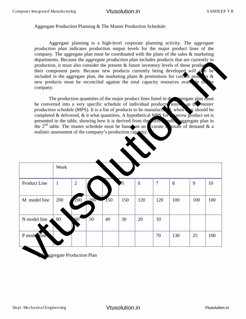
Aggregate Production Planning & The Master Production Schedule:
Aggregate planning is a high-level corporate planning activity. The aggregate
production plan indicates production output levels for the major product lines of the company. The aggregate plan must be coordinated with the plans of the sales & marketing departments. Because the aggregate production plan includes products that are currently in production, it must also consider the present & future inventory levels of those products & their component parts. Because new products currently being developed will also be included in the aggregate plan, the marketing plans & promotions for current products & new products must be reconciled against the total capacity resources available to the company.
The production quantities of the major product lines listed in the aggregate plan must be converted into a very specific schedule of individual products, known as the master
production schedule (MPS). It is a list of products to be manufactured, when they should be completed & delivered, & it what quantities. A hypothetical MPS for a narrow product set is presented in the table, showing how it is derived from the corresponding aggregate plan in the 2nd table. The master schedule must be based on an accurate estimate of demand & arealistic assessment of the company’s production capacity.
Week
Product Line 1 2 3 4 5 6 7 8 9 10
M model line 200 200 200 150 150 120 120 100 100 100
N model line 80 60 50 40 30 20 10
P model line 70 130 25 100
(a) Aggregate Production Plan
Computer Integrated Manufacturing SANDEEP T R
Dept. Mechanical Engineering Vtusolution.in
Vtusolution.in
Vtusolution.in
vtuso
lution
.in
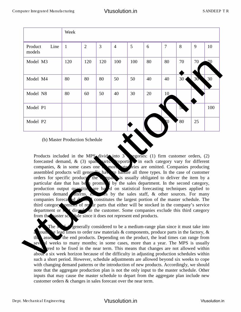
(b) Master Production Schedule
Products included in the MPS divide into 3 categories: (1) firm customer orders, (2) forecasted demand, & (3) spare parts. Proportions in each category vary for different companies, & in some cases one or more categories are omitted. Companies producing assembled products will generally have to handle all three types. In the case of customer orders for specific products, the company is usually obligated to deliver the item by a particular date that has been promised by the sales department. In the second category, production output quantities are based on statistical forecasting techniques applied to previous demand patterns, estimates by the sales staff, & other sources. For many companies forecasted demand constitutes the largest portion of the master schedule. The third category consists of repair parts that either will be stocked in the company’s service department or sent directly to the customer. Some companies exclude this third category from the master schedule since it does not represent end products.
The MPS is generally considered to be a medium-range plan since it must take into account the lead times to order raw materials & components, produce parts in the factory, & then assemble the end products. Depending on the product, the lead times can range from several weeks to many months; in some cases, more than a year. The MPS is usually considered to be fixed in the near term. This means that changes are not allowed within about a six week horizon because of the difficulty in adjusting production schedules within such a short period. However, schedule adjustments are allowed beyond six weeks to cope with changing demand patterns or the introduction of new products. Accordingly, we should note that the aggregate production plan is not the only input to the master schedule. Other inputs that may cause the master schedule to depart from the aggregate plan include new customer orders & changes in sales forecast over the near term.
Week
Product Line models
1 2 3 4 5 6 7 8 9 10
Model M3 120 120 120 100 100 80 80 70 70 70
Model M4 80 80 80 50 50 40 40 30 30 30
Model N8 80 60 50 40 30 20 10
Model P1 50 100
Model P2 70 80 25
Computer Integrated Manufacturing SANDEEP T R
Dept. Mechanical Engineering Vtusolution.in
Vtusolution.in
Vtusolution.in
vtuso
lution
.in
Material Requirements Planning:
Material Requirements Planning (MRP) is a computational technique that converts the master schedule for end products into a detailed schedule for the raw materials & components used in the end products. The detailed schedule identifies the quantities of each raw material & component item. It also indicates when each item must be ordered & delivered to meet the master schedule for final products. MRP is often thought of as a method of inventory control. It is both an effective tool for minimizing unnecessary inventory investment & a useful method in production scheduling & purchasing of materials.
The distinction between independent demand & dependent demand is important in MRP. Independent demand means that demand for a product is unrelated to demand for other items. Final products & spare parts are examples of items whose demand is independent. Independent demand patterns must usually be forecasted. Dependent demand means that demand for the item is directly related to the demand for some other item, usually a final product. The dependency usually derives from the fact that the item is a component of the other product. Component parts, raw materials, & subassemblies are examples of items subject to dependent demand.
Whereas demand for the firm’s end products must often be forecasted, the raw materials & component parts used in the end products should not be forecasted. Once the delivery schedule for the end products is established, the requirements for components & raw materials can be directly calculated. For example, even though demand for automobiles in a given month can only be forecasted, once the quantity is established & production is scheduled, we know that five tires will be needed to deliver the car (don’t forget the spare). MRP is the appropriate technique for determining quantities of dependent demand items. These items constitute the inventory of manufacturing: raw materials, work-in-process (WIP), component parts & subassemblies. That is why MRP is such a powerful technique in planning & control of manufacturing inventories. For independent demand items, inventory control is often accomplished using order point systems.
The concept of MRP is relatively straightforward. Its implementation is complicated by the sheer magnitude of the data to be processed. The master schedule provides the overall production plan for the final products in terms of month-by-month deliveries. Each product may contain hundreds of individual components. These components are produced from raw materials, some of which are common among the components. For example, several components may be made out of the same gauge sheet steel. The components are assembled into simple subassemblies, & these subassemblies are put together into more complex subassemblies, & so on, until the final products are assembled. Each step in the manufacturing & assembly sequence takes time. All of these factors must be incorporated into the MRP calculations. Although each calculation is uncomplicated, the magnitude of the date is so large that the application of MRP is practically impossible except by computer processing.
Computer Integrated Manufacturing SANDEEP T R
Dept. Mechanical Engineering Vtusolution.in
Vtusolution.in
Vtusolution.in
vtuso
lution
.in

Inputs to the MRP system :
To function, the MRP program needs data contained in several files. These files server as inputs to the MRP processor. They are (1) the master production schedule, (2) the bill of materials file and other engineering and manufacturing data, and (3) the inventory record file. Figure 1 illustrates the flow of data into the MRP processor and its conversation into useful output report. In a properly implemented MRP system, capacity planning also provides input to ensure that the MRP schedule does not exceed the production capacity of the firm. This concept is elaborated further.
The MPS lists what end products and how many of each are to be produced and when they are to be ready for shipment. Manufacturing firms generally work on monthly delivery schedules, but the master schedule in our figure uses weeks as the time periods. Whatever the duration, these time periods are called time buckets in MRP. Instead of treating time as a continuous variable ( which of course , it is ), MRP makes its computations of materials and parts requirements in terms of the buckets.
The bill of material ( BOM ) file provides information the product structure by listing the components parts and subassemblies that make up each product, It is use to computer the raw material and components requirement for end products listed in the master schedule. The structure of an assembled product can be illustrated as in Figure 2. This is much simpler than most commercial products, but its simplicity will server for illustration purposes. Product PI is composed of two subassemblies, SI and S@, each of which is made up of components C1,C2 and C3, and C3, and C4,C5 and C6, respectively. Finally, at the the bottom level are the raw materials that go into each component. The items at each successively higher level are called the parents of the items feeding into it form below. For example. SI is the parent of C1 ,C2 and C3. The product structure must also specify the number of each subassembly , component, and raw material that go into respective parent. These numbers are shown in parentheses in our figure.
Computer Integrated Manufacturing SANDEEP T R
Dept. Mechanical Engineering Vtusolution.in
Vtusolution.in
Vtusolution.in
vtuso
lution
.in
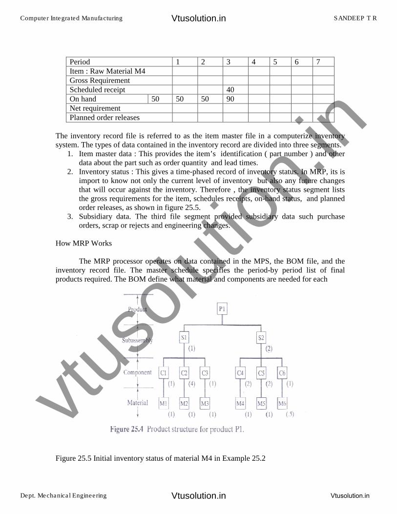
The inventory record file is referred to as the item master file in a computerize inventory system. The types of data contained in the inventory record are divided into three segments.
1. Item master data : This provides the item’s identification ( part number ) and otherdata about the part such as order quantity and lead times.
2. Inventory status : This gives a time-phased record of inventory status. In MRP, its isimport to know not only the current level of inventory but also any future changesthat will occur against the inventory. Therefore , the inventory status segment liststhe gross requirements for the item, schedules receipts, on-hand status, and plannedorder releases, as shown in figure 25.5.
3. Subsidiary data. The third file segment provided subsidiary data such purchaseorders, scrap or rejects and engineering changes.
How MRP Works
The MRP processor operates on data contained in the MPS, the BOM file, and the inventory record file. The master schedule specifies the period-by period list of final products required. The BOM define what material and components are needed for each
Figure 25.5 Initial inventory status of material M4 in Example 25.2
Period 1 2 3 4 5 6 7
Item : Raw Material M4
Gross Requirement
Scheduled receipt 40
On hand 50 50 50 90
Net requirement
Planned order releases
Computer Integrated Manufacturing SANDEEP T R
Dept. Mechanical Engineering Vtusolution.in
Vtusolution.in
Vtusolution.in
vtuso
lution
.in
Product and inventory record files gives the current and future inventory status of each product, component, and material. The MRP processor computers how many of each component and raw material are needed each period by “ exploding “ the end product requirements into successively lower levels in the product structure.
Example 25.1 MRP Gross Quantity Computations
In the master schedule of Figure 25.2, 50 units of product PI are to be completed in week 8. Explode this product requirement into the corresponding number of subassemblies and components required.
Solution : Referring to the product structure in Figure 25.4, 50 units of P1 explode into 50 units of S1 and 100 units of S2. Similarly, the requirements for these subassemblies explode into 50 units of C1, 200 of C2, 50 of C3, 200 of C5 and 100 of C6. Quantities of raw materials are determined in a similar manner.
Several complicating factors must be considered during the MRP computations. First the quantities of component and subassemblies listed in the solution of Example 25.1 do not account for any of those items that may already be stocked in inventory or are expected to be received as future order. Accordingly, the computed quantities must be adjusted for any inventories on hand or on order, a procedure called netting. For each time bucket, net requirements = gross requirements less on hand inventories and less quantities on order.
Second, quantities of common use items must be combined during parts explosion to determine the total quantities required for each component and raw material in the schedule. Common use items are raw materials and components that are used on more than one product. MRP collects these common use items from different products to achieve economics in ordering the raw materials and producing the components.
Third, lead times for each item must be taken into account, The lead time for a job is the time that must be allowed to complete the job from start to finish. There are two kinds of lead times in MRP: ordering lead timed and manufacturing lead times. Ordering lead time for an item is the time required from initiation of the purchase requisition to receipt of the item from the vendor. If the item is raw material that is stocked by the vendor, the ordering lead time should be relatively short, perhaps a few days or a few weeks. If the items is fabricated, the lead time may be substantial, perhaps several months. Manufacturing lead time is the time required to produce the item in the company’s own plant, form order release to completion, once the raw material for the item are available. The scheduled delivery of end product must be translated into time-phased requirements for components and materials by factoring in the ordering and manufacturing lead time.
EXAMPLE 25.2 MRP Time Phased Quantity Requirements :
To illustrate these various complicating factors, let use consider the MRP procedure for component C4, which is used in product P1. This part also happens to be used on product P2 of the master schedule in Figure 25.2. The product structure for P2 is shown in figure 5.6. Component C4 is made out of material M4, one unit of M4 for each unit of C4, and the inventory status of M4 is given in figure 25.5. the lead time and inventory status for each of the other items needed in the MRP calculations are shown in the table below. Complete the
Computer Integrated Manufacturing SANDEEP T R
Dept. Mechanical Engineering Vtusolution.in
Vtusolution.in
Vtusolution.in
vtuso
lution
.in
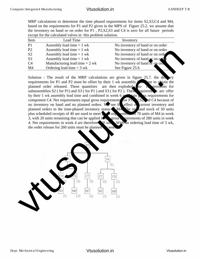
MRP calculations to determine the time phased requirements for items S2,S3,C4 and M4, based on the requirements for P1 and P2 given in the MPS of Figure 25.2. we assume that the inventory on hand or on order for P1 , P2,S2,S3 and C4 is zero for all future periods except for the calculated valves in this problem solution.
Item Lead Time Inventory
P1 Assembly lead time = 1 wk No inventory of hand or on order P2 Assembly lead time = 1 wk No inventory of hand or on order S2 Assembly lead time = 1 wk No inventory of hand or on order S3 Assembly lead time = 1 wk No inventory of hand or on order C4 Manufacturing lead time = 2 wk No inventory of hand or on order M4 Ordering lead time = 3 wk See Figure 25.6
Solution : The result of the MRP calculations are given in figure 25.7. the delivery requirements for P1 and P2 must be offset by their 1 wk assembly lead time to obtain the planned order released. These quantities are then exploded into requirements for subassemblies S2 ( for P1) and S3 ( for P1 ) and S3 ( for P2 ). These requirements are offer by their 1 wk assembly lead time and combined in week 6 to obtain gross requirements for component C4. Net requirements equal gross requirements for P1, P2,S2 and C4 because of no inventory on hand and no planned orders. We see the effect of current inventory and planned orders in the time-phased inventory status of M4. The on-hand stock of 50 units plus scheduled receipts of 40 are used to meet gross requirements of 70 units of M4 in week 3, with 20 units remaining that can be applied to the gross requirements of 280 units in week 4. Net requirements in week 4 are therefore 260 units. With an ordering lead time of 3 wk,the order release for 260 units must be planned for week 1.
Computer Integrated Manufacturing SANDEEP T R
Dept. Mechanical Engineering Vtusolution.in
Vtusolution.in
Vtusolution.in
vtuso
lution
.in
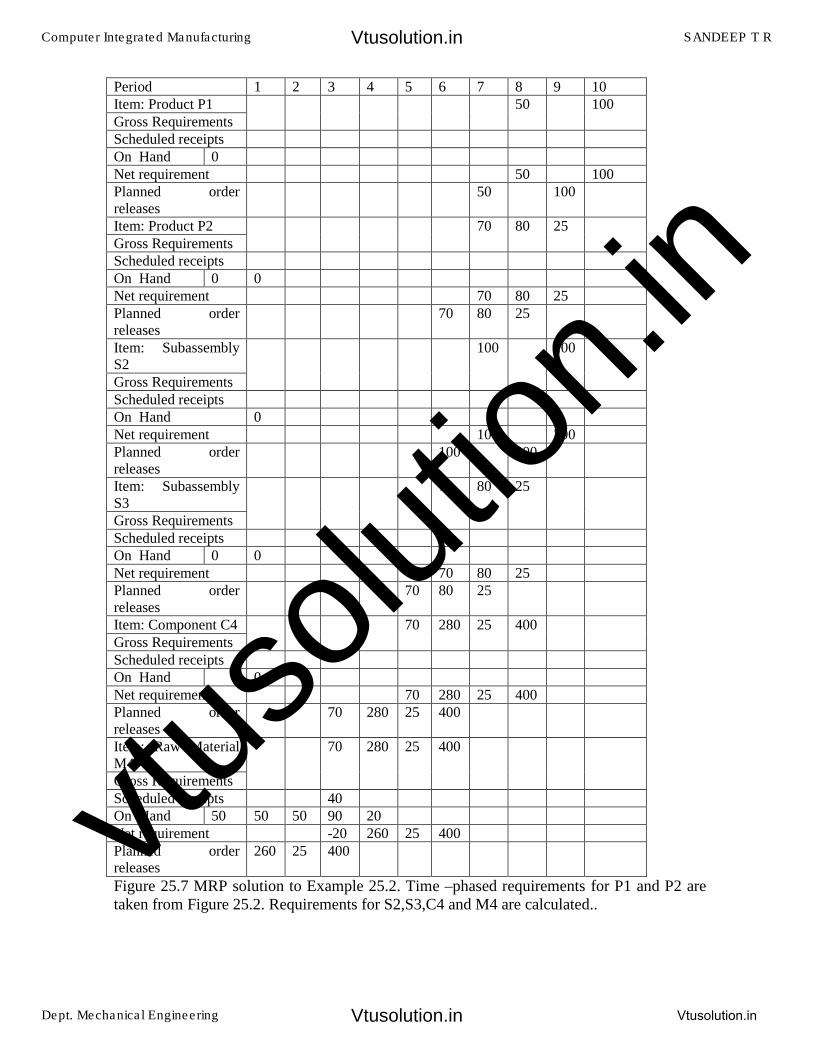
Period 1 2 3 4 5 6 7 8 9 10
Item: Product P1 50 100
Gross Requirements
Scheduled receipts
On Hand 0
Net requirement 50 100
Planned order releases
50 100
Item: Product P2 70 80 25
Gross Requirements
Scheduled receipts
On Hand 0 0
Net requirement 70 80 25
Planned order releases
70 80 25
Item: Subassembly S2
100 200
Gross Requirements
Scheduled receipts
On Hand 0
Net requirement 100 200
Planned order releases
100 200
Item: Subassembly S3
70 80 25
Gross Requirements
Scheduled receipts
On Hand 0 0
Net requirement 70 80 25
Planned order releases
70 80 25
Item: Component C4 70 280 25 400
Gross Requirements
Scheduled receipts
On Hand 0
Net requirement 70 280 25 400
Planned order releases
70 280 25 400
Item: Raw Material M4
70 280 25 400
Gross Requirements
Scheduled receipts 40
On Hand 50 50 50 90 20
Net requirement -20 260 25 400
Planned order releases
260 25 400
Figure 25.7 MRP solution to Example 25.2. Time –phased requirements for P1 and P2 are taken from Figure 25.2. Requirements for S2,S3,C4 and M4 are calculated..
Computer Integrated Manufacturing SANDEEP T R
Dept. Mechanical Engineering Vtusolution.in
Vtusolution.in
Vtusolution.in
vtuso
lution
.in
25.2.3. MRP Output and Benefits :
The MRP program generates a variety of outputs that can be used in planning and managing plant operations. The ouput include (1) planned order releases, which provide the authority to place orders that have been planned by the MRP system: (2) report of planned order releases in future periods ; (3) rescheduling notices, indicating changes in due dates for open orders; (4) cancellation notices, indicating that certain open orders have been canceled because in the MPS;(5) reports on inventory status; (6) performance reports of various types , indicating costs, item usage, actual versus planned lead times, and so on; (7) exception report , showing deviations from the schedule from the schedule, orders thatare overdue, scrap, and so on; and (8) inventory forecasts, indicating projected inventorylevels in future periods.
Of the MRP output listed above, the planned order releases are the most important because they drive the production system. Planned order of two kinds, purchase orders and work orders. Purchase orders provide the authority to purchase raw materials or parts from outside vendors, with quantities and delivery dates specified. Work orders generate the authority to produce parts or assembly subassemblies or products in the company’s own factory. Again , quantities to be completed and completion dates are specified.
Benefits reported by users of MRP systems include the following: (1) reduction in inventory, (2) quicker response to changes in demand than is possible with a manual requirements planning systems, (3) reduced setup and product changeover costs, (4) better machine utilization, (5) improved capacity to respond to changes in the master schedule, and (6) aid in developing the master schedule.
Notwithstanding these claimed benefits, the success rate in implementing MRP systems throughout industry has been less than perfect. Some MRP systems have not been successful because (1) the application was not appropriate, usually because the product structure did not fit the data requirements of MRP; (2) the MRP computations were based on inaccurate data; and (3) the MPS was not coupled with a capacity planning system, so the MRP program generated an unrealistic schedule of work orders that overloaded the factory.
25.3 CAPACITY PLANNING :
The original MRP system that were developed in the 1970s created schedules that were not necessarily consists with the production capabilities and limitations of the plants that were to produce the products. In many instances, the MRP system developed the detailed schedule based on a master production schedule that was unrealistic. A successful production schedule must consider production capacity. In cases where current capacity is inadequate, the firm must make plans for changes in capacity to meet the changing production requirements specified in the schedule. In chapter 3, we defined production capacity and formulated equations to determine the capacity of a plant. Capacity planning consists of determining what labor and equipment resources are required to meet the current MPS as well as long term future production needs of the firm ( see Advanced Manufacturing Planning, Section 24.4 ). Capacity planni9ng also identifies the limitations of the available production resources to prevent the MRP program from planning an un realistic master schedule.
Computer Integrated Manufacturing SANDEEP T R
Dept. Mechanical Engineering Vtusolution.in
Vtusolution.in
Vtusolution.in
vtuso
lution
.in
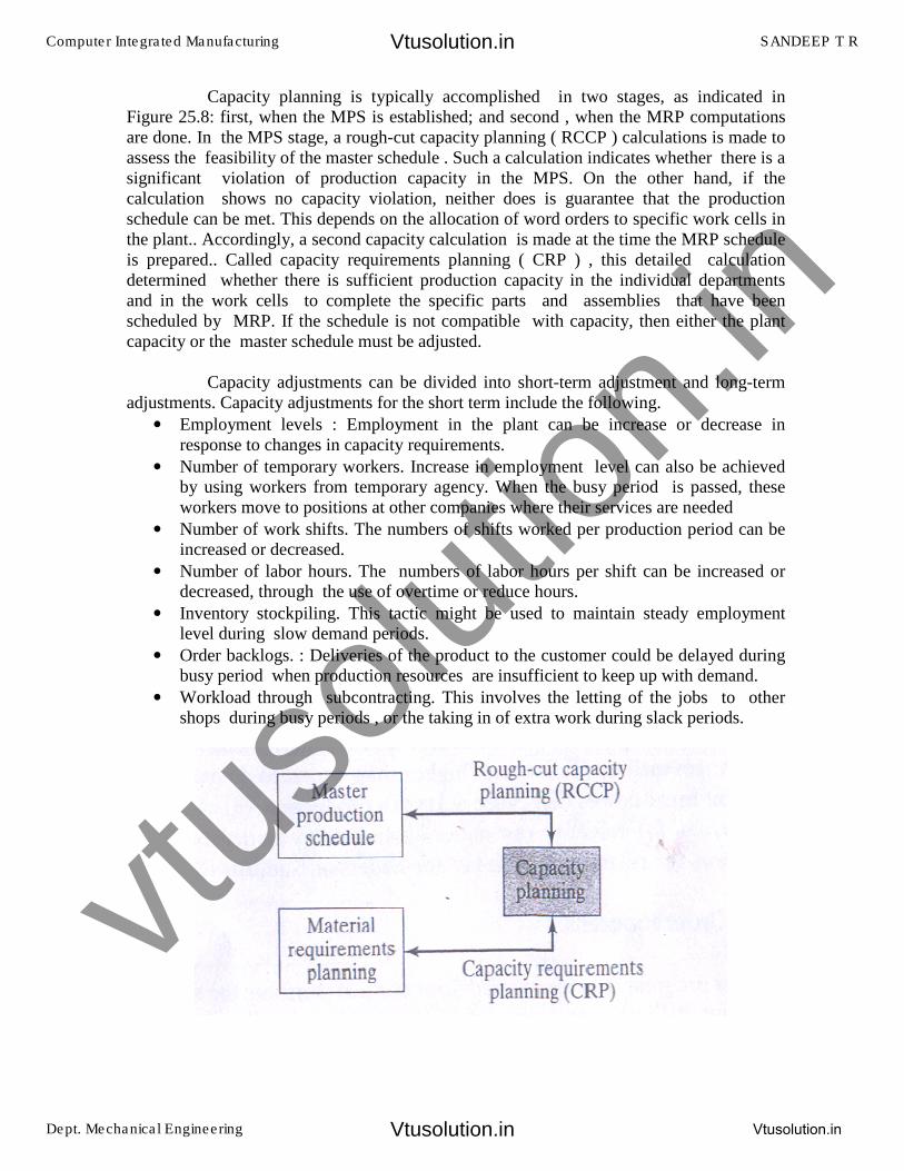
Capacity planning is typically accomplished in two stages, as indicated in Figure 25.8: first, when the MPS is established; and second , when the MRP computations are done. In the MPS stage, a rough-cut capacity planning ( RCCP ) calculations is made to assess the feasibility of the master schedule . Such a calculation indicates whether there is a significant violation of production capacity in the MPS. On the other hand, if the calculation shows no capacity violation, neither does is guarantee that the production schedule can be met. This depends on the allocation of word orders to specific work cells in the plant.. Accordingly, a second capacity calculation is made at the time the MRP schedule is prepared.. Called capacity requirements planning ( CRP ) , this detailed calculation determined whether there is sufficient production capacity in the individual departments and in the work cells to complete the specific parts and assemblies that have been scheduled by MRP. If the schedule is not compatible with capacity, then either the plant capacity or the master schedule must be adjusted.
Capacity adjustments can be divided into short-term adjustment and long-term adjustments. Capacity adjustments for the short term include the following.
• Employment levels : Employment in the plant can be increase or decrease inresponse to changes in capacity requirements.
• Number of temporary workers. Increase in employment level can also be achievedby using workers from temporary agency. When the busy period is passed, theseworkers move to positions at other companies where their services are needed
• Number of work shifts. The numbers of shifts worked per production period can beincreased or decreased.
• Number of labor hours. The numbers of labor hours per shift can be increased ordecreased, through the use of overtime or reduce hours.
• Inventory stockpiling. This tactic might be used to maintain steady employmentlevel during slow demand periods.
• Order backlogs. : Deliveries of the product to the customer could be delayed duringbusy period when production resources are insufficient to keep up with demand.
• Workload through subcontracting. This involves the letting of the jobs to othershops during busy periods , or the taking in of extra work during slack periods.
Computer Integrated Manufacturing SANDEEP T R
Dept. Mechanical Engineering Vtusolution.in
Vtusolution.in
Vtusolution.in
vtuso
lution
.in
Capacity planning adjustments for the long term include changes in production capacity that generally require long times. These adjustments include the following actions:
• Investing in new equipment. This involves investing in more machines or moreproductive machines to meet increased future production requirements, oreinvesting in new types of machines to match changes in product design.
• Constructing new plants. Building a new factory represents a major investment forthe company. However, it also represents a significant increase in productioncapacity for the firm.
• Purchasing existing plants from other companies.
• Acquiring existing companies . This may be done to increase productive capacity.However , there are usually more important reasons for taking over an existingcompany, such as to achieve economies of scale that result from increase marketshare and reducing staff.
• Closing Plants. This involves the closing of plants that will not be needed in thefuture.
Computer Integrated Manufacturing SANDEEP T R
Dept. Mechanical Engineering Vtusolution.in
Vtusolution.in
Vtusolution.in
vtuso
lution
.in
Unit -7 :
CNC MACHINING CENTERS
INTRODUCTION TO COMPUTER NUMERICAL CONTROL
The variety being demanded in view of the varying tastes of the consumer calls for a very small batch sizes. Small batch sizes will not be able to take advantage of the mass production techniques such as special purpose machines or transfer lines. Hence, the need for flexible automation is felt , where you not only get the benefits of rigid automation but are also able to vary the products manufactured thus bringing in the flexibility. Numerical control fits the bill perfectly and we would see that manufacturing would increasingly be dependent on numerical control in future.
Numerical control
Numerical control of machine tools may be defined as a method of automation in which various functions of machine tools are controlled by letters, numbers and symbols. Basically a NC machine runs on a program fed to it. The program consists of precise instructions about the methodology of manufacture as well as movements. For example, what tool is to be used, at what speed, at what feed and to move from which point to which point in what path. Since the program is the controlling point for product manufacture, the machine becomes versatile and can be used for any part. All the functions of a NC machine tool are therefore controlled electronically, hydraulically or pneumatically. In NC machine tools, one or more of the following functions may be automatic.
a. Starting and stopping of machine tool spindle.
b. Controlling the spindle speed.
c. Positioning the tool tip at desired locations and guiding it along desired paths byautomatic control of motion of slides.
d. Controlling the rate of movement of tool tip ( feed rate)
e. Changing of tools in the spindle.
Functions of a machine tool
The purpose of a machine tool is to cut away surplus material, usually metal from the material supplied to leave a work piece of the required shape and size, produced to an acceptable degree of accuracy and surface finish. The machine tool should possess certain capabilities in order to fulfill these requirements. It must be
Computer Integrated Manufacturing SANDEEP T R
Dept. Mechanical Engineering Vtusolution.in
Vtusolution.in
Vtusolution.in
vtuso
lution
.in
a. Able to hold the work piece and cutting tool securely.
b. Endowed the sufficient power to enable the tool to cut the work piece material ateconomical rates.
c. Capable of displacing the tool and work piece relative to one another to produce therequired work piece shape. The displacements must be controlled with a degree ofprecision which will ensure the desired accuracy of surface finish and size.
Concept of numerical control
Formerly, the machine tool operator guided a cutting tool around a work piece by manipulating hand wheels and dials to get a finished or somewhat finished part. In his procedure many judgments of speeds, feeds, mathematics and sometimes even tool configuration were his responsibility. The number of judgments the machinist had to make usually depended on the type of stock he worked in and the kind of organization that prevailed. If his judgment was an error, it resulted in rejects or at best parts to be reworked or repaired in some fashion.
Decisions concerning the efficient and correct use of the machine tool then depended on the craftsmanship, knowledge and skill of the machinist himself. It is rare that two expert operators produced identical parts using identical procedure and identical judgment of speeds, feeds and tooling. In fact even one craftsman may not proceed in same manner the second time around.
. Process planners and programmers have now the responsibilities for these matters.
It must be understood that NC does not alter the capabilities of the machine tool. The With NC the correct and most efficient use of a machine no longer rests with the
operator.Actual machine tool with a capable operator can do nothing more than it was capable of doing before a MCU was joined to it. New metal removing principles are not involved. Cutting speeds, feeds and tooling principles must still be adhered to. The advantage is idle time is reduced and the actual utilization rate is mush higher (compresses into one or two years that a conventional machine receives in ten years).
Historical Development
1947 was the year in which Numerical control was born. It began because of an urgent need. John C Parsons of the parson’s corporation, Michigan, a manufacturer of helicopter rotor blades could not make his templates fast enough. so he invented a way of coupling computer equipment with a jig borer.
Computer Integrated Manufacturing SANDEEP T R
Dept. Mechanical Engineering Vtusolution.in
Vtusolution.in
Vtusolution.in
vtuso
lution
.in
The US air force realized in 1949 that parts for its planes and missiles were becoming more complex. Also the designs were constantly being improved; changes in drawings were frequently made. Thus in their search for methods of speeding up production, an air force study contract was awarded to the Parson’s Corporation. The servomechanisms lab of MIT was the subcontractor.
In 1951, the MIT took over the complete job and in 1952; a prototype of NC machine was successfully demonstrated. The term “Numerical Control” was coined at MIT. In 1955 seven companies had tape controlled machines. In 1960, there were 100 NC machines at the machine tool shown in Chicago and a majority of them were relatively simple point to point application.
During these years the electronics industry was busy. First miniature electronic tubes were developed, then solid state circuitry and then modular or integrated circuits. Thus the reliability of the controls has been greatly increased and they have become most compact and less expensive.
Today there are several hundred sizes and varieties of machines, many options and many varieties of control system available.
Definition:
The simplest definition is as the name implies, “a process a controlled by numbers “. Numerical Control is a system in which the direct insertions of programmed numerical value, stored on some form of input medium are automatically read and decoded to cause a corresponding function on the machine tool which it is controlling.
Advantages of NC machine tools:
1. Reduced lead time:
Lead time includes the time needed for planning, design and manufacture of jigs, etc. This time may amount to several months. Since the need for special jigs and fixtures is often entirely eliminated, the whole time needed for their design and manufacture is saved.
2. Elimination of operator errors:
The machine is controlled by instructions registered on the tape provided the tape is correct and machine and tool operate correctly, no errors will occur in the job. Fatigue, boredom, or inattention by operator will not affect the quality or duration of the machining. Responsibility is transferred from the operator to the tape, machine settings are achieved without the operator reading the dial.
Computer Integrated Manufacturing SANDEEP T R
Dept. Mechanical Engineering Vtusolution.in
Vtusolution.in
Vtusolution.in
vtuso
lution
.in
3. Operator activity:
The operator is relieved of tasks performed by the machine and is free to attend to matters for which his skills and ability are essential. Presetting of tools, setting of components and preparation and planning of future jobs fall into this category. It is possible for two work stations to be prepared on a single machine table, even with small batches. Two setting positions are used, and the operator can be setting one station while machining takes place at the other.
4. Lower labor cost
More time is actually spent on cutting the metal. Machine manipulation time ex.:. Gear changing and often setting time are less with NC machines and help reduce the labor cost per job considerably.
5. Smaller batches
By the use of preset tooling and presetting techniques downtime between batches is kept at a minimum. Large storage facilities for work in progress are not required. Machining centers eliminate some of the setups needed for a succession of operation on one job; time spent in waiting until each of a succession of machine is free is also cut. The components circulate round the machine shop in a shorter period, inter department costs are saved and ‘program chasing’ is reduced.
6. Longer tool life
Tools can be used at optimum speeds and feeds because these functions are controlled by the program.
7. Elimination of special jigs and fixtures
Because standard locating fixtures are often sufficient of work on machines. the cost of special jigs and fixture is frequently eliminated. The capital cost of storage facilities is greatly reduced. The storage of a tape in a simple matter, it may be kept for many years and manufacturing of spare parts, repeat orders or replacements is made much more convenient.
8. Flexibility in changes of component design
The modification of component design can be readily accommodated by reprogramming and altering the tape. Savings are affected in time and cost.
9. Reduced inspection.
The time spent on inspection and in waiting for inspection to begin is greatly reduced. Normally it is necessary to inspect the first component only once the tape is proved; the repetitive accuracy of the machine maintains a consistent product.
Computer Integrated Manufacturing SANDEEP T R
Dept. Mechanical Engineering Vtusolution.in
Vtusolution.in
Vtusolution.in
vtuso
lution
.in
10. Reduced scrap
Operator error is eliminated and a proven tape results in accurate component.
11. Accurate costing and scheduling
The time taken in machining is predictable, consistent and results in a greater accuracy in estimating and more consistency in costing.
Evolution of CNC:
With the availability of microprocessors in mid 70’s the controller technology has made a tremendous progress. The new control systems are termed as computer numerical control (CNC) which are characterized by the availability of a dedicated computer and enhanced memory in the controller. These may also be termed “soft wired numerical control”.
There are many advantages which are derived from the use of CNC as compared to NC.
• Part program storage memory.
• Part program editing.
• Part program downloading and uploading.
• Part program simulation using tool path.
• Tool offset data and tool life management.
• Additional part programming facilities.
• Macros and subroutines.
• Background tape preparation, etc.
The controls with the machine tools these days are all CNC and the old NC control do not exist any more.
Computer Integrated Manufacturing SANDEEP T R
Dept. Mechanical Engineering Vtusolution.in
Vtusolution.in
Vtusolution.in
vtuso
lution
.in
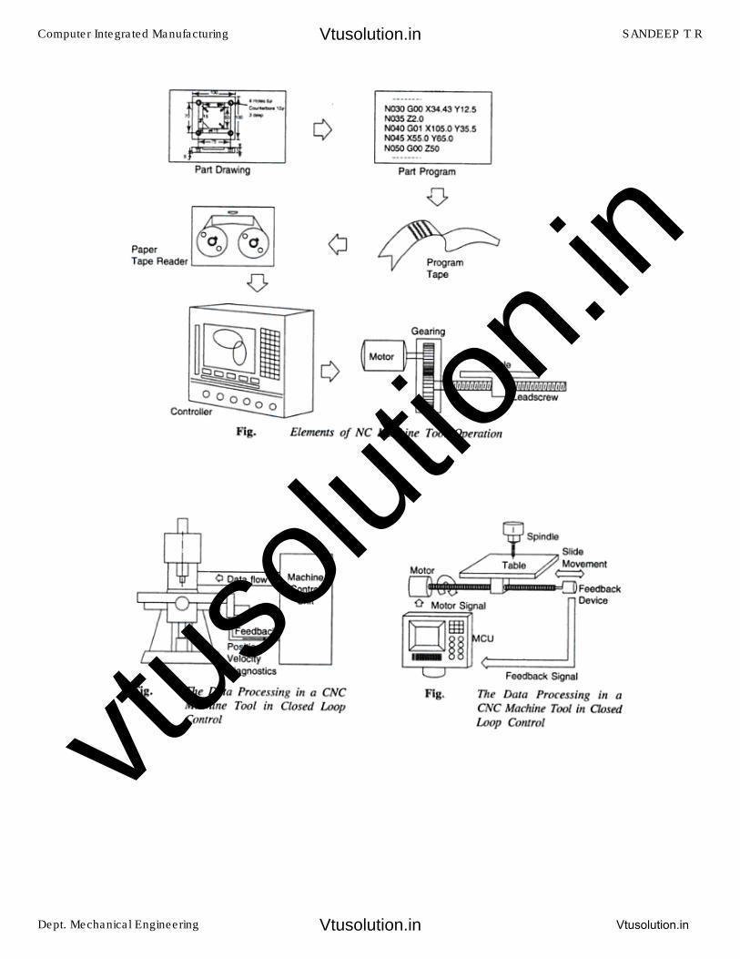
Computer Integrated Manufacturing SANDEEP T R
Dept. Mechanical Engineering Vtusolution.in
Vtusolution.in
Vtusolution.in
vtuso
lution
.in
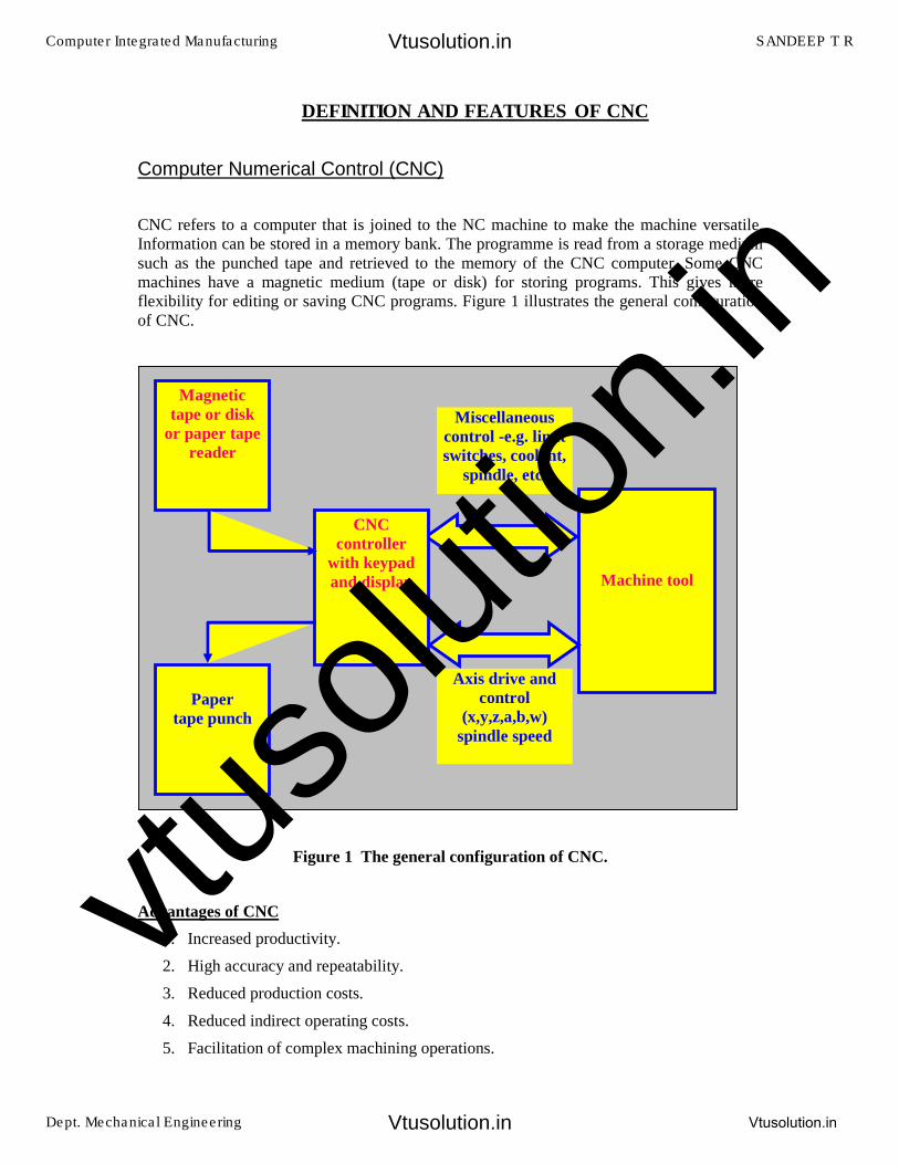
DEFINITION AND FEATURES OF CNC
Computer Numerical Control (CNC)
CNC refers to a computer that is joined to the NC machine to make the machine versatile. Information can be stored in a memory bank. The programme is read from a storage medium such as the punched tape and retrieved to the memory of the CNC computer. Some CNC machines have a magnetic medium (tape or disk) for storing programs. This gives more flexibility for editing or saving CNC programs. Figure 1 illustrates the general configuration of CNC.
Figure 1 The general configuration of CNC.
Advantages of CNC
1. Increased productivity.
2. High accuracy and repeatability.
3. Reduced production costs.
4. Reduced indirect operating costs.
5. Facilitation of complex machining operations.
Machine tool
Miscellaneous
control -e.g. limit
switches, coolant,
spindle, etc.
Axis drive and
control
(x,y,z,a,b,w)
spindle speed
CNC
controller
with keypad
and display
Magnetic
tape or disk
or paper tape
reader
Paper
tape punch����
Computer Integrated Manufacturing SANDEEP T R
Dept. Mechanical Engineering Vtusolution.in
Vtusolution.in
Vtusolution.in
vtuso
lution
.in
6. Greater flexibility.
7. Improved production planning and control.
8. Lower operator skill requirement.
9. Facilitation of flexible automation.
Limitations of CNC:
1. High initial investment.
2. High maintenance requirement.
3. Not cost-effective for low production cost.
Features of CNC
Computer NC systems include additional features beyond what is feasible with conventional hard-wired NC. These features, many of which are standard on most CNC Machine Control units (MCU), include the following:
• Storage of more than one part program : With improvements in computer storagetechnology, newer CNC controllers have sufficient capacity to store multipleprograms. Controller manufacturers generally offer one or more memory expansionsas options to the MCU
• Various forms of program input : Whereas conventional (hard-wired) MCUs arelimited to punched tape as the input medium for entering part programs, CNCcontrollers generally possess multiple data entry capabilities, such as punched tape,magnetic tape, floppy diskettes, RS-232 communications with external computers,and manual data input (operator entry of program).
• Program editing at the machine tool : CNC permits a part program to be editedwhile it resides in the MCU computer memory. Hence, a part program can be testedand corrected entirely at the machine site, rather than being returned to theprogramming office for corrections. In addition to part program corrections, editingalso permits cutting conditions in the machining cycle to be optimized. After theprogram has been corrected and optimized, the revised version can be stored onpunched tape or other media for future use.
• Fixed cycles and programming subroutines : The increased memory capacity andthe ability to program the control computer provide the opportunity to store frequentlyused machining cycles as macros, that can be called by the part program. Instead ofwriting the full instructions for the particular cycle into every program, a programmerincludes a call statement in the part program to indicate that the macro cycle shouldbe executed. These cycles often require that certain parameters be defined, for
Computer Integrated Manufacturing SANDEEP T R
Dept. Mechanical Engineering Vtusolution.in
Vtusolution.in
Vtusolution.in
vtuso
lution
.in
example, a bolt hole circle, in which the diameter of the bolt circle, the spacing of the bolt holes, and other parameters must be specified.
• Interpolation : Some of the interpolation schemes are normally executed only on aCNC system because of computational requirements. Linear and circular interpolationare sometimes hard-wired into the control unit, but helical, parabolic, and cubicinterpolations are usually executed by a stored program algorithm.
• Positioning features for setup : Setting up the machine tool for a given workpartinvolves installing and aligning a fixture on the machine tool table. This must beaccomplished so that the machine axes are established with respect to the workpart.The alignment task can be facilitated using certain features made possible by softwareoptions in the CNC system. Position set is one of the features. With position set, theoperator is not required to locate the fixture on the machine table with extremeaccuracy. Instead, the machine tool axes are referenced to the location of the fixtureusing a target point or set of target points on the work or fixture.
• Cutter length and size compensation : In older style controls, cutter dimensionshade to be set precisely to agree with the tool path defined in the part program.Alternative methods for ensuring accurate tool path definition have been incorporatedinto the CNC controls. One method involves manually entering the actual tooldimensions into the MCU. These actual dimensions may differ from those originallyprogrammed. Compensations are then automatically made in the computed tool path.Another method involves use of a tool length sensor built into the machine. In thistechnique, the cutter is mounted in the spindle and the sensor measures its length. Thismeasured value is then used to correct the programmed tool path.
• Acceleration and deceleration calculations : This feature is applicable when thecutter moves at high feed rates. It is designed to avoid tool marks on the work surfacethat would be generated due to machine tool dynamics when the cutter path changesabruptly. Instead, the feed rate is smoothly decelerated in anticipation of a tool pathchange and then accelerated back up to the programmed feed rate after the directionchange.
• Communications interface : With the trend toward interfacing and networking inplants today, most modern CNC controllers are equipped with a standard RS-232 orother communications interface to link the machine to other computers and computer-driven devices. This is useful for various applications, such as (1)downloading partprograms from a central data file; (2)collecting operational data such as workpiececounts, cycle times, and machine utilization; and (3)interfacing with peripheralequipment, such as robots that unload and load parts.
Computer Integrated Manufacturing SANDEEP T R
Dept. Mechanical Engineering Vtusolution.in
Vtusolution.in
Vtusolution.in
vtuso
lution
.in
• Diagnostics : Many modern CNC systems possess a diagnostics capability thatmonitors certain aspects of the machine tool to detect malfunctions or signs ofimpending malfunctions or to diagnose system breakdowns.
The Machine Control Unit (MCU) for CNC
The MCU is the hardware that distinguishes CNC from conventional NC. The general configuration of the MCU in a CNC system is illustrated in Figure 2. The MCU consists of the following components and subsystems: (1) Central Processing Unit, (2) Memory, (3) Input/Output Interface, (4) Controls for Machine Tool Axes and Spindle Speed, and (5) Sequence Controls for Other Machine Tool Functions. These subsystems are interconnected by means of a system bus, which communicates data and signals among the components of a network.
• Central Processing Unit : The central processing unit (CPU) is the brain of the MCU. Itmanages the other components in the MCU based on software contained in main memory.The CPU can be divided into three sections: (1) control section, (2) arithmetic-logic unit,and (3) immediate access memory. The control section retrieves commands and data frommemory and generates signals to activate other components in the MCU. In short, itsequences, coordinates, and regulates all the activities of the MCU computer. Thearithmetic-logic unit (ALU) consists of the circuitry to perform various calculations(addition, subtraction, multiplication), counting, and logical functions required bysoftware residing in memory. The immediate access memory provides a temporarystorage of data being processed by the CPU. It is connected to main memory of thesystem data bus.
• Memory : The immediate access memory in the CPU is not intended for storing CNCsoftware. A much greater storage capacity is required for the various programs and dataneeded to operate the CNC system. As with most other computer systems, CNC memorycan be divided into two categories: (1) primary memory, and (2) secondary memory.Main memory (also known as primary storage) consists of ROM (read-only memory) andRAM (random access memory) devices. Operating system software and machineinterface programs are generally stored in ROM. These programs are usually installed bythe manufacturer of the MCU. Numerical control part programs are stored in RAMdevices. Current programs in RAM can be erased and replaced by new programs as jobsare changed.
Computer Integrated Manufacturing SANDEEP T R
Dept. Mechanical Engineering Vtusolution.in
Vtusolution.in
Vtusolution.in
vtuso
lution
.in
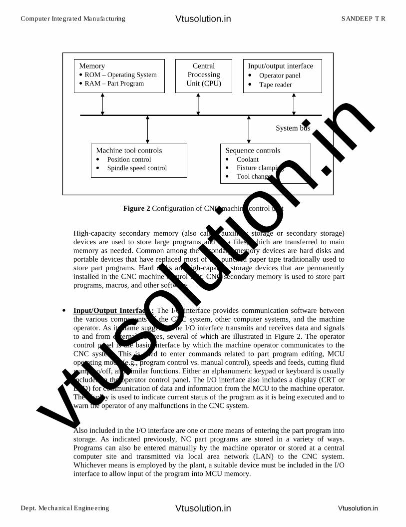
Figure 2 Configuration of CNC machine control unit
High-capacity secondary memory (also called auxiliary storage or secondary storage) devices are used to store large programs and data files, which are transferred to main memory as needed. Common among the secondary memory devices are hard disks and portable devices that have replaced most of the punched paper tape traditionally used to store part programs. Hard disks are high-capacity storage devices that are permanently installed in the CNC machine control unit. CNC secondary memory is used to store part programs, macros, and other software.
• Input/Output Interface : The I/O interface provides communication software betweenthe various components of the CNC system, other computer systems, and the machineoperator. As its name suggests, The I/O interface transmits and receives data and signalsto and from external devices, several of which are illustrated in Figure 2. The operatorcontrol panel is the basic interface by which the machine operator communicates to theCNC system. This is used to enter commands related to part program editing, MCUoperating mode (e.g., program control vs. manual control), speeds and feeds, cutting fluidpump on/off, and similar functions. Either an alphanumeric keypad or keyboard is usuallyincluded in the operator control panel. The I/O interface also includes a display (CRT orLED) for communication of data and information from the MCU to the machine operator.The display is used to indicate current status of the program as it is being executed and towarn the operator of any malfunctions in the CNC system.
Also included in the I/O interface are one or more means of entering the part program into storage. As indicated previously, NC part programs are stored in a variety of ways. Programs can also be entered manually by the machine operator or stored at a central computer site and transmitted via local area network (LAN) to the CNC system. Whichever means is employed by the plant, a suitable device must be included in the I/O interface to allow input of the program into MCU memory.
Memory • ROM – Operating System
• RAM – Part Program
Central Processing Unit (CPU)
Input/output interface
• Operator panel
• Tape reader
Machine tool controls • Position control
• Spindle speed control
Sequence controls • Coolant
• Fixture clamping
• Tool changer
System bus
Computer Integrated Manufacturing SANDEEP T R
Dept. Mechanical Engineering Vtusolution.in
Vtusolution.in
Vtusolution.in
vtuso
lution
.in
• Controls for Machine Tool Axes and Spindle Speed : These are hardware componentsthat control the position and velocity (feed rate) of each machine axis as well as therotational speed of the machine tool spindle. The control signals generated by MCU mustbe converted to a form and power level suited to the particular position control systemsused to drive the machine axes. Positioning systems can be classified as open loop orclosed loop, and different hardware components are required in each case.
Depending on the type of machine tool, the spindle is used to drive either (1) workpiece or (2) a rotating cutter. Turning exemplifies the first case, whereas milling and drilling exemplify the second. Spindle speed is a programmed parameter for most CNC machine tools. Spindle speed components in the MCU usually consist of s drive control circuit and a feedback sensor interface. The particular hardware components depend on the type of spindle drive.
• Sequence Controls for Other Machine Tool Functions :
In addition to control of table position, feed rate, and spindle speed, several additional functions are accomplished under part program control. These auxiliary functions are generally on/off (binary) actuations, interlocks, and discrete numerical data. To avoid overloading the CPU, a programmable logic controller is sometimes used to manage the I/O interface for these auxiliary functions.
Classification Of CNC Machine Tools
(1) Based on the motion type 'Point-to-point & Contouring systems’
There are two main types of machine tools and the control systems required for use with them differ because of the basic differences in the functions of the machines to be controlled. They are known as point-to-point and contouring controls.
(1.1)Point-to-point systems
Some machine tools for example drilling, boring and tapping machines etc, require the cutter and the work piece to be placed at a certain fixed relative positions at which they must remain while the cutter does its work. These machines are known as point-to-point machines as shown in figure 3 (a) and the control equipment for use with them are known as point-to-point control equipment. Feed rates need not to be programmed. In these machine tools, each axis is driven separately. In a point-to-point control system, the dimensional information that must be given to the machine tool will be a series of required position of the two slides. Servo systems can be used to move the slides and no attempt is made to move the slide until the cutter has been retracted back.
Computer Integrated Manufacturing SANDEEP T R
Dept. Mechanical Engineering Vtusolution.in
Vtusolution.in
Vtusolution.in
vtuso
lution
.in
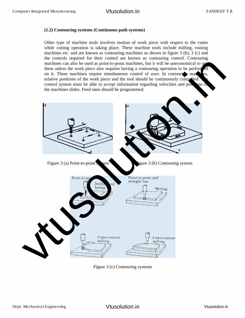
(1.2) Contouring systems (Continuous path systems)
Other type of machine tools involves motion of work piece with respect to the cutter while cutting operation is taking place. These machine tools include milling, routing machines etc. and are known as contouring machines as shown in figure 3 (b), 3 (c) and the controls required for their control are known as contouring control. Contouring machines can also be used as point-to-point machines, but it will be uneconomical to use them unless the work piece also requires having a contouring operation to be performed on it. These machines require simultaneous control of axes. In contouring machines, relative positions of the work piece and the tool should be continuously controlled. The control system must be able to accept information regarding velocities and positions of the machines slides. Feed rates should be programmed.
Figure 3 (a) Point-to-point system Figure 3 (b) Contouring system
Figure 3 (c) Contouring systems
Computer Integrated Manufacturing SANDEEP T R
Dept. Mechanical Engineering Vtusolution.in
Vtusolution.in
Vtusolution.in
vtuso
lution
.in

(2) Based on the control loops ‘Open loop & Closed loop systems’
(2.1) Open loop systems (Fig 4(a)):
Programmed instructions are fed into the controller through an input device. These instructions are then converted to electrical pulses (signals) by the controller and sent to the servo amplifier to energize the servo motors. The primary drawback of the open-loop system is that there is no feedback system to check whether the program position and velocity has been achieved. If the system performance is affected by load, temperature, humidity, or lubrication then the actual output could deviate from the desired output. For these reasons the open -loop system is generally used in point-to-point systems where the accuracy requirements are not critical. Very few continuous-path systems utilize open-loop control.
Figure 4(a) Open loop control system Figure 4(b) Closed loop control system
(2.2) Closed loop systems (Fig 4(b)):
The closed-loop system has a feedback subsystem to monitor the actual output and correct any discrepancy from the programmed input. These systems use position and velocity feed back. The feedback system could be either analog or digital. The analog systems measure the variation of physical variables such as position and velocity in terms of voltage levels. Digital systems monitor output variations by means of electrical pulses. To control the dynamic behavior and the final position of the machine slides, a variety of position transducers are employed. Majority of CNC systems operate on servo mechanism, a closed loop principle. If a discrepancy is revealed between where the machine element should be and where it actually is, the sensing device signals the driving unit to make an adjustment, bringing the movable component to the required location. Closed-loop systems are very powerful and accurate because they are capable of monitoring operating conditions through feedback subsystems and automatically compensating for any variations in real-time.
Computer Integrated Manufacturing SANDEEP T R
Dept. Mechanical Engineering Vtusolution.in
Vtusolution.in
Vtusolution.in
vtuso
lution
.in
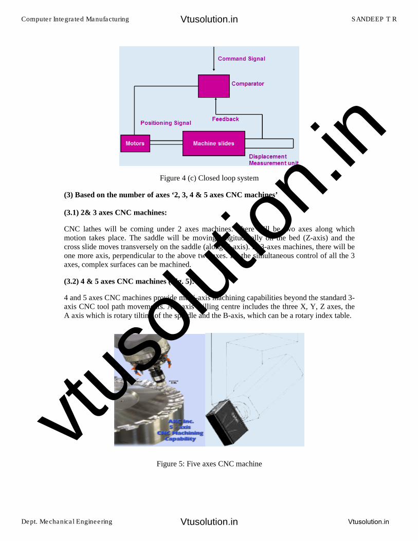
Figure 4 (c) Closed loop system
(3) Based on the number of axes ‘2, 3, 4 & 5 axes CNC machines’
(3.1) 2& 3 axes CNC machines:
CNC lathes will be coming under 2 axes machines. There will be two axes along which motion takes place. The saddle will be moving longitudinally on the bed (Z-axis) and the cross slide moves transversely on the saddle (along X-axis). In 3-axes machines, there will be one more axis, perpendicular to the above two axes. By the simultaneous control of all the 3 axes, complex surfaces can be machined.
(3.2) 4 & 5 axes CNC machines (Fig. 5):
4 and 5 axes CNC machines provide multi-axis machining capabilities beyond the standard 3-axis CNC tool path movements. A 5-axis milling centre includes the three X, Y, Z axes, the A axis which is rotary tilting of the spindle and the B-axis, which can be a rotary index table.
Figure 5: Five axes CNC machine
Computer Integrated Manufacturing SANDEEP T R
Dept. Mechanical Engineering Vtusolution.in
Vtusolution.in
Vtusolution.in
vtuso
lution
.in
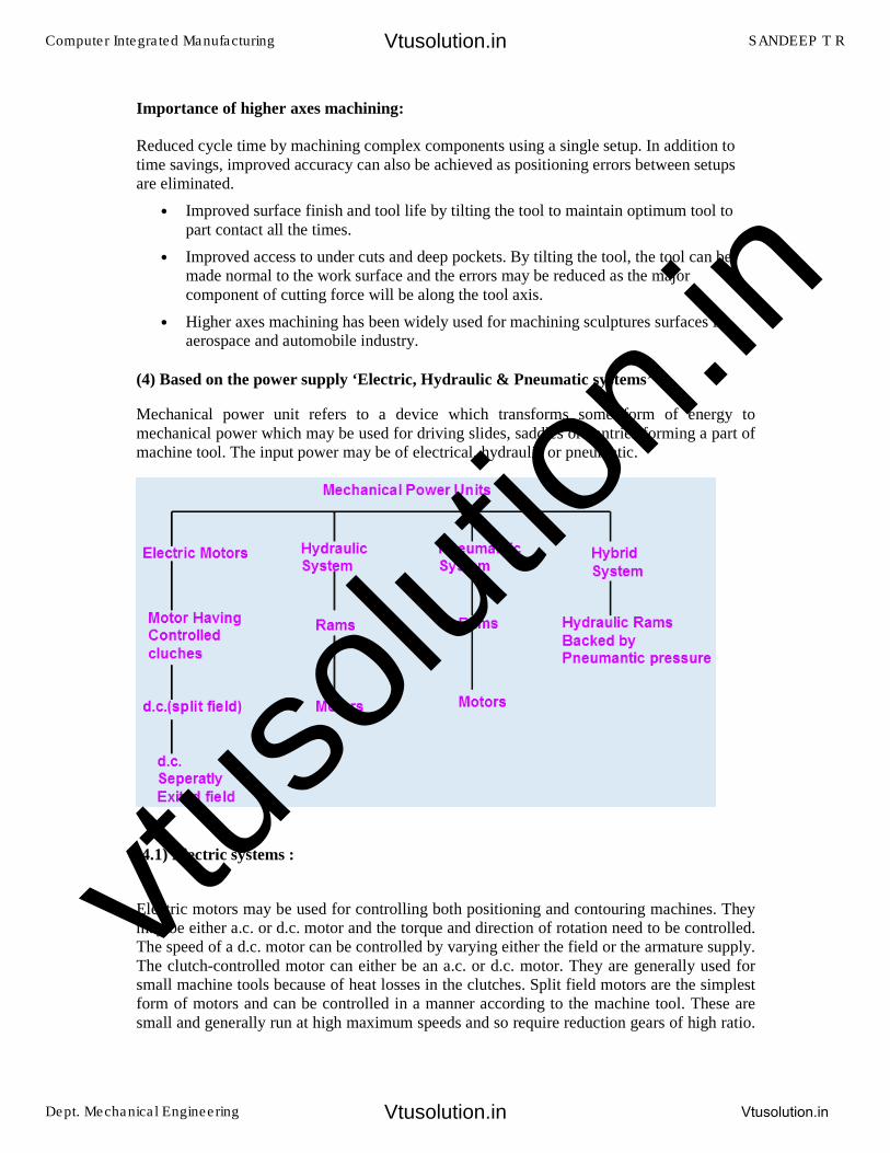
Importance of higher axes machining:
Reduced cycle time by machining complex components using a single setup. In addition to time savings, improved accuracy can also be achieved as positioning errors between setups are eliminated.
• Improved surface finish and tool life by tilting the tool to maintain optimum tool topart contact all the times.
• Improved access to under cuts and deep pockets. By tilting the tool, the tool can bemade normal to the work surface and the errors may be reduced as the majorcomponent of cutting force will be along the tool axis.
• Higher axes machining has been widely used for machining sculptures surfaces inaerospace and automobile industry.
(4) Based on the power supply ‘Electric, Hydraulic & Pneumatic systems’
Mechanical power unit refers to a device which transforms some form of energy to mechanical power which may be used for driving slides, saddles or gantries forming a part of machine tool. The input power may be of electrical, hydraulic or pneumatic.
(4.1) Electric systems :
Electric motors may be used for controlling both positioning and contouring machines. They may be either a.c. or d.c. motor and the torque and direction of rotation need to be controlled. The speed of a d.c. motor can be controlled by varying either the field or the armature supply. The clutch-controlled motor can either be an a.c. or d.c. motor. They are generally used for small machine tools because of heat losses in the clutches. Split field motors are the simplest form of motors and can be controlled in a manner according to the machine tool. These are small and generally run at high maximum speeds and so require reduction gears of high ratio.
Computer Integrated Manufacturing SANDEEP T R
Dept. Mechanical Engineering Vtusolution.in
Vtusolution.in
Vtusolution.in
vtuso
lution
.in
Separately excited motors are used with control systems for driving the slides of large machine tools.
(4.2) Hydraulic systems:
These hydraulic systems may be used with positioning and contouring machine tools of all sizes. These systems may be either in the form of rams or motors. Hydraulic motors are smaller than electric motors of equivalent power. There are several types of hydraulic motors. The advantage of using hydraulic motors is that they can be very small and have considerable torque. This means that they may be incorporated in servosystems which require having a rapid response.
Computer Integrated Manufacturing SANDEEP T R
Dept. Mechanical Engineering Vtusolution.in
Vtusolution.in
Vtusolution.in
vtuso
lution
.in
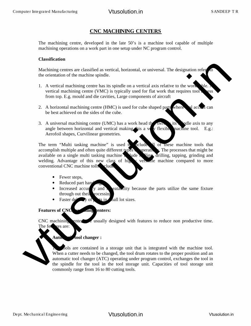
CNC MACHINING CENTERS
The machining centre, developed in the late 50’s is a machine tool capable of multiple machining operations on a work part in one setup under NC program control.
Classification
Machining centres are classified as vertical, horizontal, or universal. The designation refers to the orientation of the machine spindle.
1. A vertical machining centre has its spindle on a vertical axis relative to the work table. Avertical machining centre (VMC) is typically used for flat work that requires tool accessfrom top. E.g. mould and die cavities, Large components of aircraft
2. A horizontal machining centre (HMC) is used for cube shaped parts where tool access canbe best achieved on the sides of the cube.
3. A universal machining centre (UMC) has a work head that swivels its spindle axis to anyangle between horizontal and vertical making this a very flexible machine tool. E.g.:Aerofoil shapes, Curvilinear geometries.
The term “Multi tasking machine” is used to include all of these machine tools that accomplish multiple and often quite different types of operations. The processes that might be available on a single multi tasking machine include milling, drilling, tapping, grinding and welding. Advantage of this new class of highly versatile machine compared to more conventional CNC machine tolls include:
• Fewer steps,
• Reduced part handling,
• Increased accuracy and repeatability because the parts utilize the same fixturethrough out their processing
• Faster delivery of parts in small lot sizes.
Features of CNC machining centers:
CNC machining centers are usually designed with features to reduce non productive time. The features are:
• Automatic tool changer :
The tools are contained in a storage unit that is integrated with the machine tool.When a cutter needs to be changed, the tool drum rotates to the proper position and anautomatic tool changer (ATC) operating under program control, exchanges the tool inthe spindle for the tool in the tool storage unit. Capacities of tool storage unitcommonly range from 16 to 80 cutting tools.
Computer Integrated Manufacturing SANDEEP T R
Dept. Mechanical Engineering Vtusolution.in
Vtusolution.in
Vtusolution.in
vtuso
lution
.in
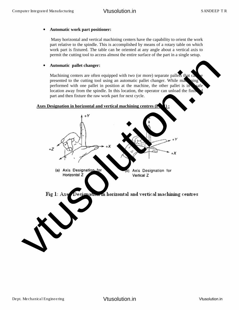
• Automatic work part positioner:
Many horizontal and vertical machining centers have the capability to orient the workpart relative to the spindle. This is accomplished by means of a rotary table on whichwork part is fixtured. The table can be oriented at any angle about a vertical axis topermit the cutting tool to access almost the entire surface of the part in a single setup.
• Automatic pallet changer:
Machining centers are often equipped with two (or more) separate pallets that can bepresented to the cutting tool using an automatic pallet changer. While machining isperformed with one pallet in position at the machine, the other pallet is in a safelocation away from the spindle. In this location, the operator can unload the finishedpart and then fixture the raw work part for next cycle.
Axes Designation in horizontal and vertical machining centres (Fig 1) :
Computer Integrated Manufacturing SANDEEP T R
Dept. Mechanical Engineering Vtusolution.in
Vtusolution.in
Vtusolution.in
vtuso
lution
.in
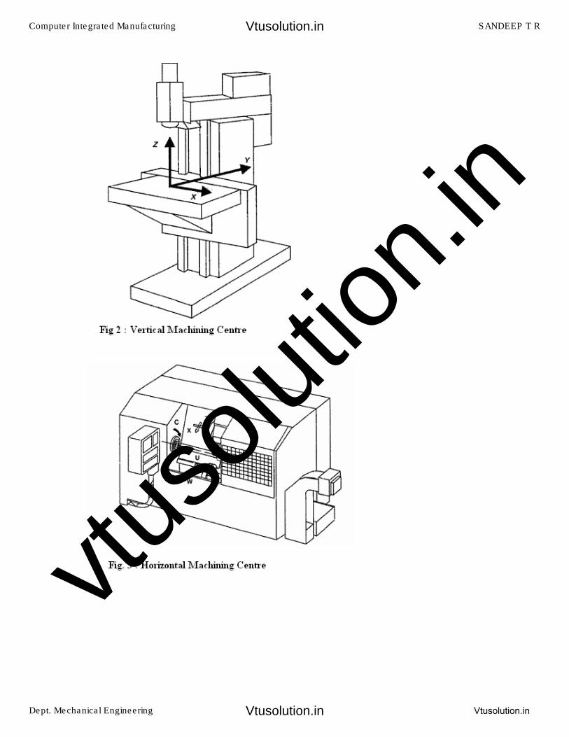
Computer Integrated Manufacturing SANDEEP T R
Dept. Mechanical Engineering Vtusolution.in
Vtusolution.in
Vtusolution.in
vtuso
lution
.in
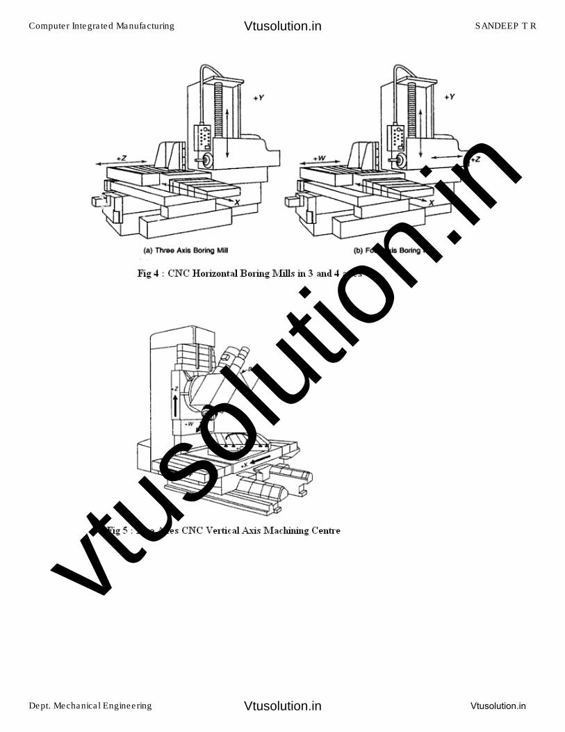
Computer Integrated Manufacturing SANDEEP T R
Dept. Mechanical Engineering Vtusolution.in
Vtusolution.in
Vtusolution.in
vtuso
lution
.in
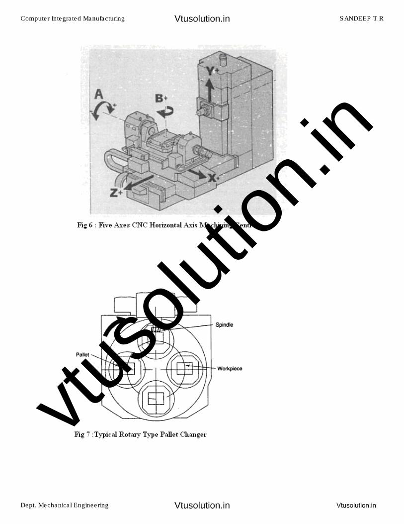
Computer Integrated Manufacturing SANDEEP T R
Dept. Mechanical Engineering Vtusolution.in
Vtusolution.in
Vtusolution.in
vtuso
lution
.in
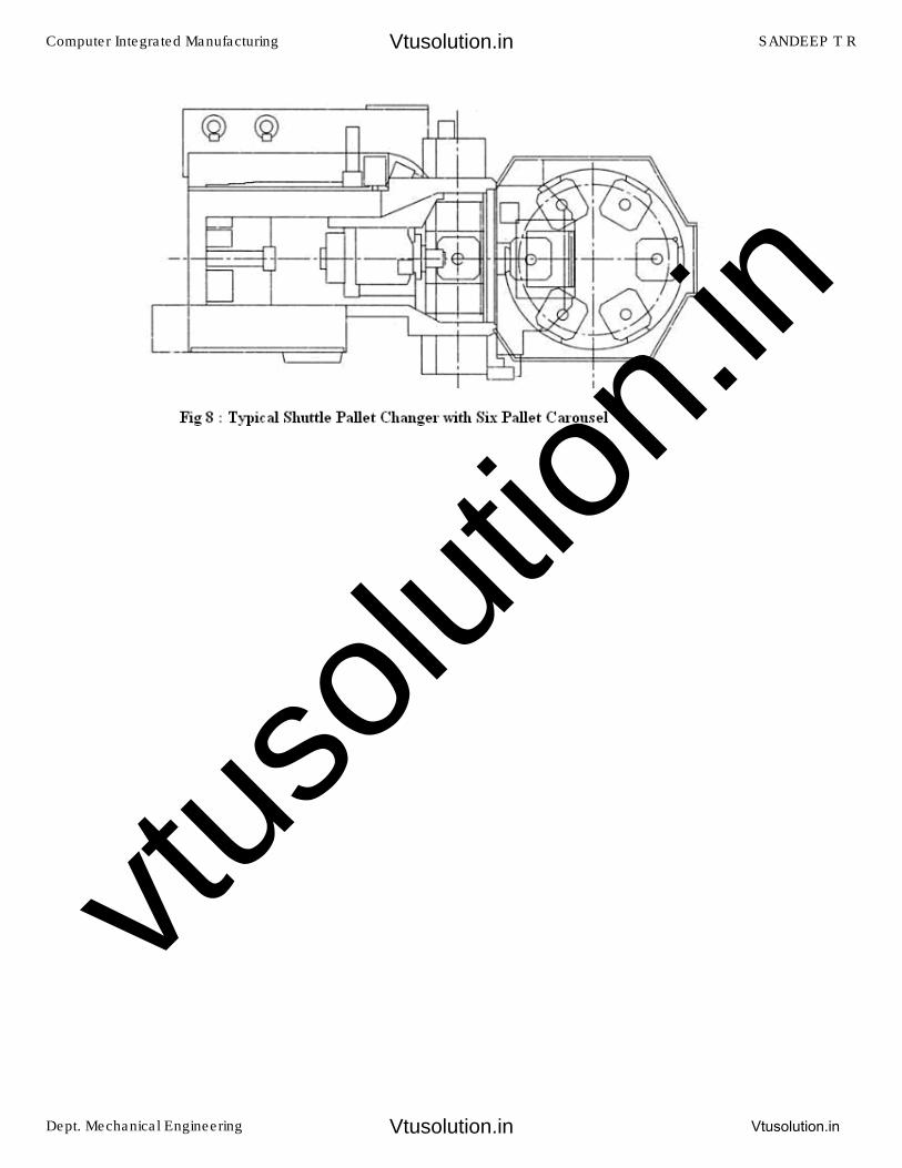
Computer Integrated Manufacturing SANDEEP T R
Dept. Mechanical Engineering Vtusolution.in
Vtusolution.in
Vtusolution.in
vtuso
lution
.in
CNC PART PROGRAMMING
(1) Programming fundamentals
Machining involves an important aspect of relative movement between cutting tool and workpiece. In machine tools this is accomplished by either moving the tool with respect to workpiece or vice versa. In order to define relative motion of two objects, reference directions are required to be defined. These reference directions depend on type of machine tool and are defined by considering an imaginary coordinate system on the machine tool. A program defining motion of tool / workpiece in this coordinate system is known as a part program. Lathe and Milling machines are taken for case study but other machine tools like CNC grinding, CNC hobbing, CNC filament winding machine, etc. can also be dealt with in the same manner.
(1.1) Reference Point
Part programming requires establishment of some reference points. Three reference points are either set by manufacturer or user.
a) Machine Origin
The machine origin is a fixed point set by the machine tool builder. Usually it cannot be changed. Any tool movement is measured from this point. The controller always remembers tool distance from the machine origin.
b) Program Origin
It is also called home position of the tool. Program origin is point from where the tool starts for its motion while executing a program and returns back at the end of the cycle. This can be any point within the workspace of the tool which is sufficiently away from the part. In case of CNC lathe it is a point where tool change is carried out.
c) Part Origin
The part origin can be set at any point inside the machine's electronic grid system. Establishing the part origin is also known as zero shift, work shift, floating zero or datum. Usually part origin needs to be defined for each new setup. Zero shifting allows the relocation of the part. Sometimes the part accuracy is affected by the location of the part origin. Figure 1 and 2 shows the reference points on a lathe and milling machine.
Computer Integrated Manufacturing SANDEEP T R
Dept. Mechanical Engineering Vtusolution.in
Vtusolution.in
Vtusolution.in
vtuso
lution
.in
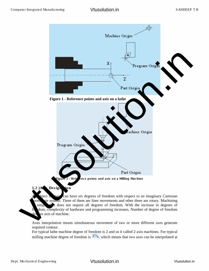
Figure 1 - Reference points and axis on a lathe
Figure 2 - Reference points and axis on a Milling Machine
1.2 )Axis Designation
An object in space can have six degrees of freedom with respect to an imaginary Cartesian coordinate system. Three of them are liner movements and other three are rotary. Machining of simple part does not require all degrees of freedom. With the increase in degrees of freedom, complexity of hardware and programming increases. Number of degree of freedom defines axis of machine.
Axes interpolation means simultaneous movement of two or more different axes generate required contour. For typical lathe machine degree of freedom is 2 and so it called 2 axis machines. For typical
milling machine degree of freedom is , which means that two axes can be interpolated at
Computer Integrated Manufacturing SANDEEP T R
Dept. Mechanical Engineering Vtusolution.in
Vtusolution.in
Vtusolution.in
vtuso
lution
.in
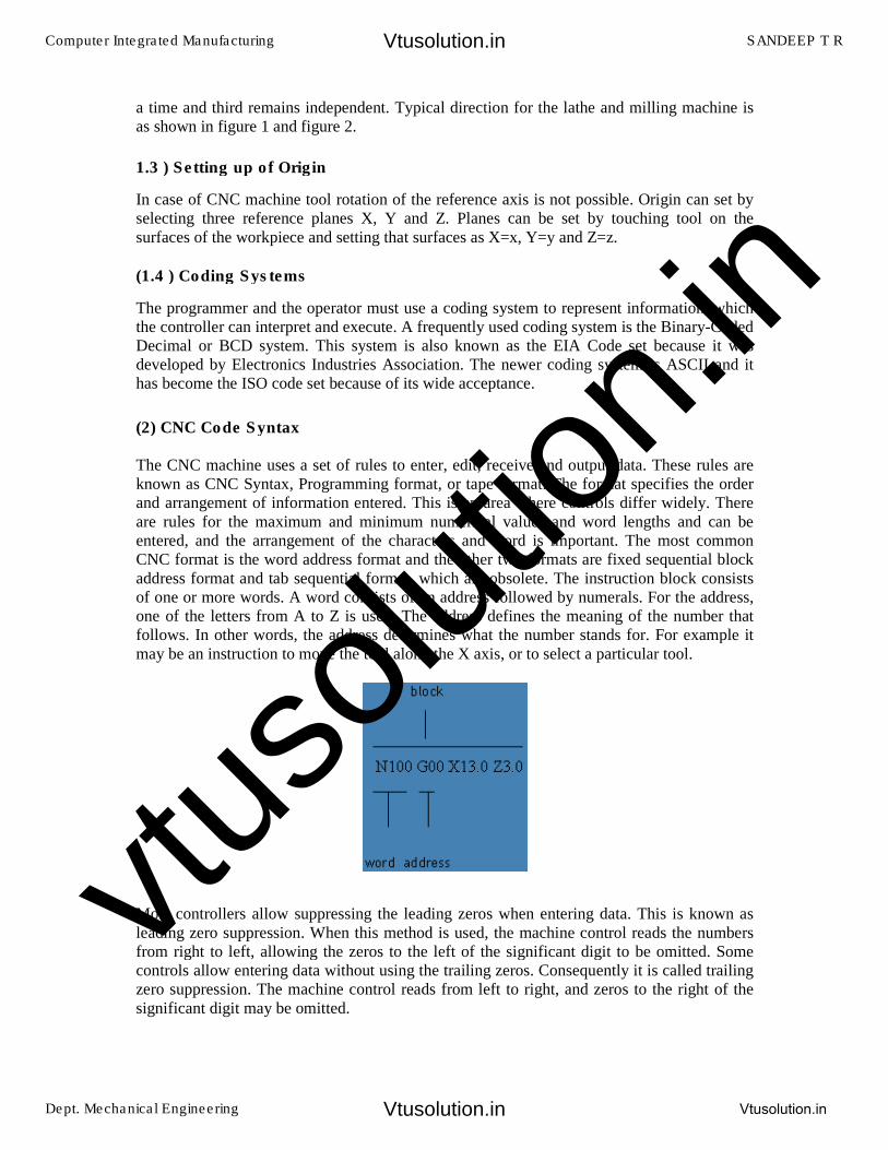
a time and third remains independent. Typical direction for the lathe and milling machine is as shown in figure 1 and figure 2.
1.3 ) Setting up of Origin
In case of CNC machine tool rotation of the reference axis is not possible. Origin can set by selecting three reference planes X, Y and Z. Planes can be set by touching tool on the surfaces of the workpiece and setting that surfaces as X=x, Y=y and Z=z.
(1.4 ) Coding Systems
The programmer and the operator must use a coding system to represent information, which the controller can interpret and execute. A frequently used coding system is the Binary-Coded Decimal or BCD system. This system is also known as the EIA Code set because it was developed by Electronics Industries Association. The newer coding system is ASCII and it has become the ISO code set because of its wide acceptance.
(2) CNC Code Syntax
The CNC machine uses a set of rules to enter, edit, receive and output data. These rules are known as CNC Syntax, Programming format, or tape format. The format specifies the order and arrangement of information entered. This is an area where controls differ widely. There are rules for the maximum and minimum numerical values and word lengths and can be entered, and the arrangement of the characters and word is important. The most common CNC format is the word address format and the other two formats are fixed sequential block address format and tab sequential format, which are obsolete. The instruction block consists of one or more words. A word consists of an address followed by numerals. For the address, one of the letters from A to Z is used. The address defines the meaning of the number that follows. In other words, the address determines what the number stands for. For example it may be an instruction to move the tool along the X axis, or to select a particular tool.
Most controllers allow suppressing the leading zeros when entering data. This is known as leading zero suppression. When this method is used, the machine control reads the numbers from right to left, allowing the zeros to the left of the significant digit to be omitted. Some controls allow entering data without using the trailing zeros. Consequently it is called trailing zero suppression. The machine control reads from left to right, and zeros to the right of the significant digit may be omitted.
Computer Integrated Manufacturing SANDEEP T R
Dept. Mechanical Engineering Vtusolution.in
Vtusolution.in
Vtusolution.in
vtuso
lution
.in
3) Types of CNC codes
(3.1) Preparatory codes
The term "preparatory" in NC means that it "prepares" the control system to be ready for implementing the information that follows in the next block of instructions. A preparatory
function is designated in a program by the word address G followed by two digits. Preparatory functions are also called G-codes and they specify the control mode of the operation.
(3.2) Miscellaneous codes
Miscellaneous functions use the address letter M followed by two digits. They perform a group of instructions such as coolant on/off, spindle on/off, tool change, program stop, or program end. They are often referred to as machine functions or M-functions. Some of the M codes are given below.
M00 Unconditional stop M02 End of program M03 Spindle clockwise M04 Spindle counterclockwise M05 Spindle stop M06 Tool change (see Note below) M30 End of program
In principle, all codes are either modal or non-modal. Modal code stays in effect until cancelled by another code in the same group. The control remembers modal codes. This gives the programmer an opportunity to save programming time. Non-modal code stays in effect only for the block in which it is programmed. Afterwards, its function is turned off automatically. For instance G04 is a non-modal code to program a dwell. After one second, which is say, the programmed dwell time in one particular case, this function is cancelled. To perform dwell in the next blocks, this code has to be reprogrammed. The control does not memorize the non-modal code, so it is called as one shot codes. One-shot commands are non-
modal. Commands known as "canned cycles" (a controller's internal set of preprogrammed subroutines for generating commonly machined features such as internal pockets and drilled holes) are non-modal and only function during the call.
On some older controllers, cutter positioning (axis) commands (e.g., G00, G01, G02, G03, & G04) are non-modal requiring a new positioning command to be entered each time the cutter (or axis) is moved to another location.
Computer Integrated Manufacturing SANDEEP T R
Dept. Mechanical Engineering Vtusolution.in
Vtusolution.in
Vtusolution.in
vtuso
lution
.in
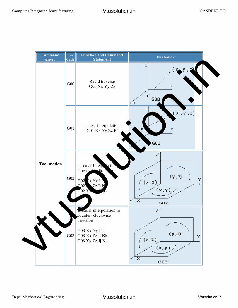
Command group
G-code
Function and Command Statement
Illustration
Tool motion
G00Rapid traverse G00 Xx Yy Zz
G01Linear interpolation G01 Xx Yy Zz Ff
G02
Circular Interpolation in clock-wise direction
G02 Xx Yy Ii Jj G02 Xx Zz Ii Kk G02 Yy Zz Jj Kk
G03
Circular interpolation in counter- clockwise direction
G03 Xx Yy Ii Jj G03 Xx Zz Ii Kk G03 Yy Zz Jj Kk
Computer Integrated Manufacturing SANDEEP T R
Dept. Mechanical Engineering Vtusolution.in
Vtusolution.in
Vtusolution.in
vtuso
lution
.in
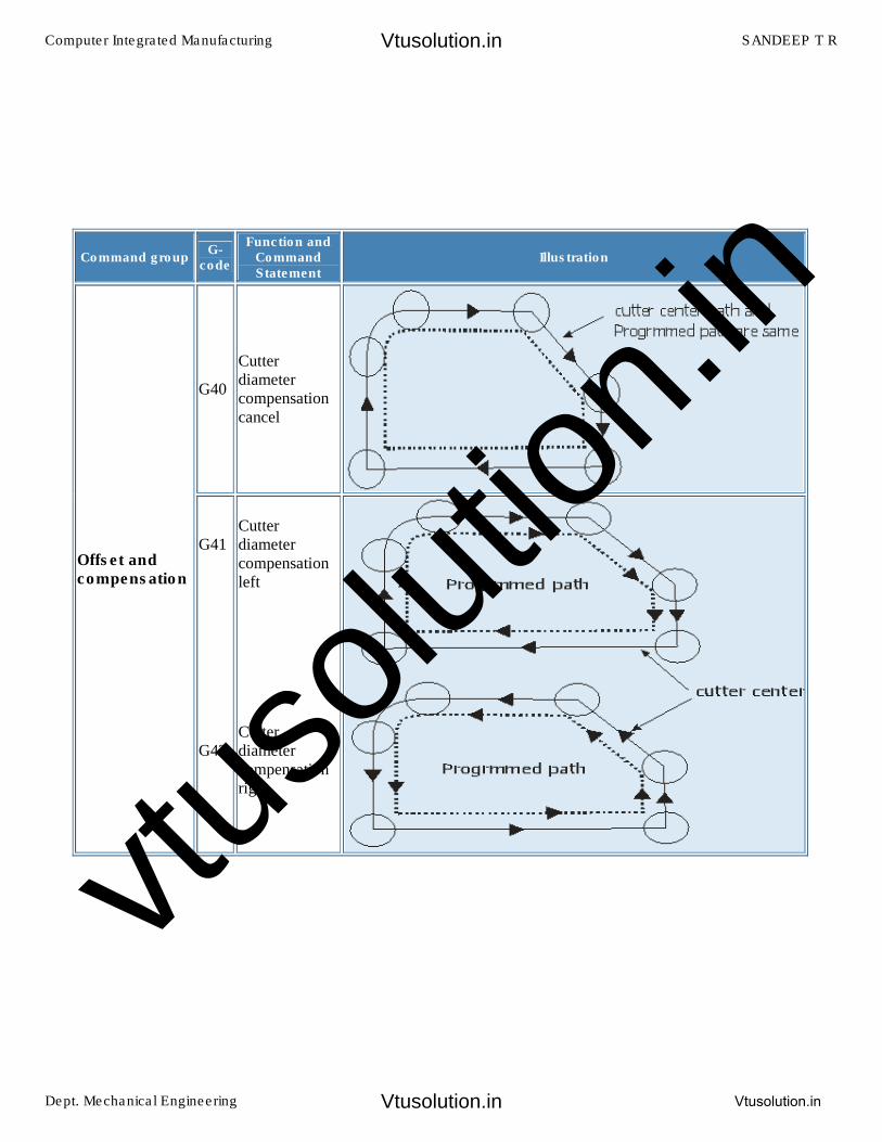
Command group G-
code
Function and Command Statement
Illustration
Offset and compensation
G40
Cutter diameter compensation cancel
G41
G42
Cutter diameter compensation left
Cutter diameter compensation right
Computer Integrated Manufacturing SANDEEP T R
Dept. Mechanical Engineering Vtusolution.in
Vtusolution.in
Vtusolution.in
vtuso
lution
.in
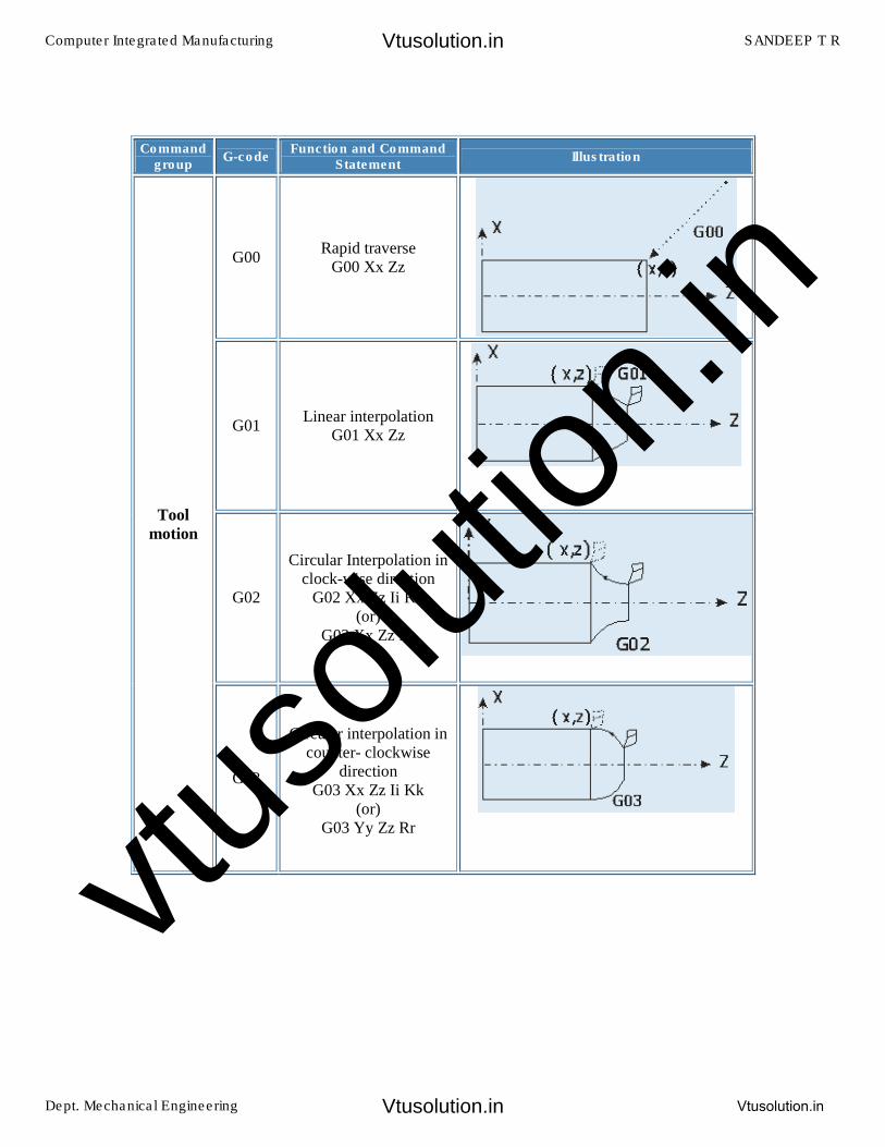
Command group
G-codeFunction and Command
Statement Illustration
Tool
motion
G00Rapid traverse
G00 Xx Zz
G01Linear interpolation
G01 Xx Zz
G02
Circular Interpolation in clock-wise direction
G02 Xx Zz Ii Kk (or)
G02 Xx Zz Rr
G03
Circular interpolation in counter- clockwise
direction G03 Xx Zz Ii Kk
(or) G03 Yy Zz Rr
Computer Integrated Manufacturing SANDEEP T R
Dept. Mechanical Engineering Vtusolution.in
Vtusolution.in
Vtusolution.in
vtuso
lution
.in
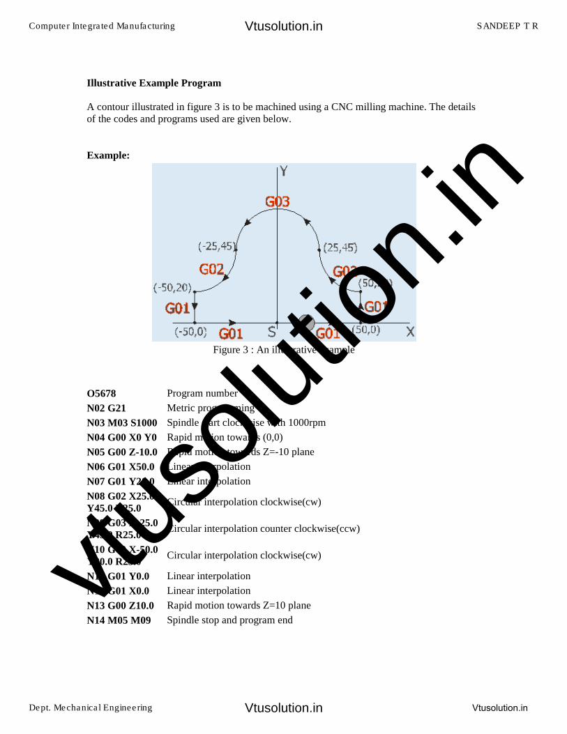
Illustrative Example Program
A contour illustrated in figure 3 is to be machined using a CNC milling machine. The details of the codes and programs used are given below.
Example:
Figure 3 : An illustrative example
O5678 Program number
N02 G21 Metric programming
N03 M03 S1000 Spindle start clockwise with 1000rpm
N04 G00 X0 Y0 Rapid motion towards (0,0)
N05 G00 Z-10.0 Rapid motion towards Z=-10 plane
N06 G01 X50.0 Linear interpolation
N07 G01 Y20.0 Linear interpolation
N08 G02 X25.0
Y45.0 R25.0 Circular interpolation clockwise(cw)
N09 G03 X-25.0
Y45.0 R25.0 Circular interpolation counter clockwise(ccw)
N10 G02 X-50.0
Y20.0 R25.0 Circular interpolation clockwise(cw)
N11 G01 Y0.0 Linear interpolation
N12 G01 X0.0 Linear interpolation
N13 G00 Z10.0 Rapid motion towards Z=10 plane
N14 M05 M09 Spindle stop and program end
Computer Integrated Manufacturing SANDEEP T R
Dept. Mechanical Engineering Vtusolution.in
Vtusolution.in
Vtusolution.in
vtuso
lution
.in
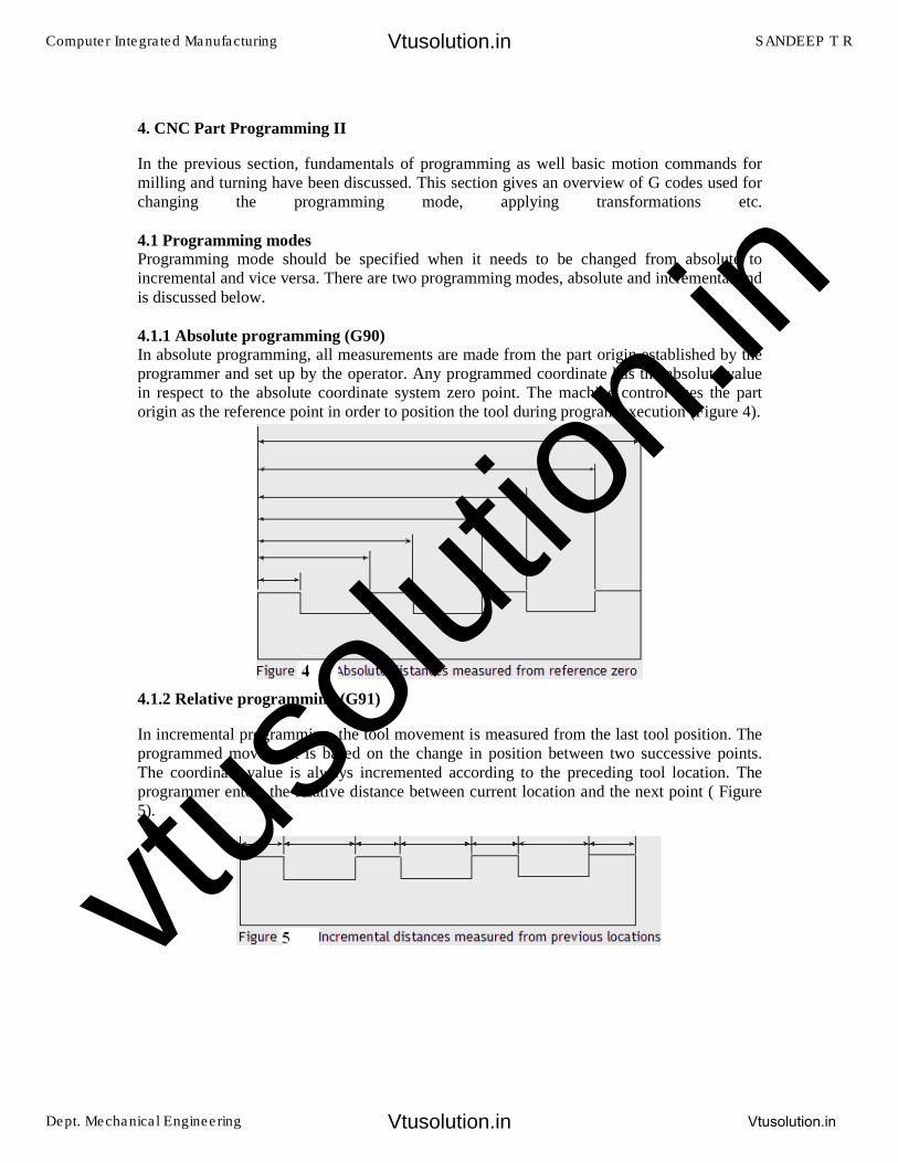
4. CNC Part Programming II
In the previous section, fundamentals of programming as well basic motion commands for milling and turning have been discussed. This section gives an overview of G codes used for changing the programming mode, applying transformations etc.
4.1 Programming modes Programming mode should be specified when it needs to be changed from absolute to incremental and vice versa. There are two programming modes, absolute and incremental and is discussed below.
4.1.1 Absolute programming (G90) In absolute programming, all measurements are made from the part origin established by the programmer and set up by the operator. Any programmed coordinate has the absolute value in respect to the absolute coordinate system zero point. The machine control uses the part origin as the reference point in order to position the tool during program execution (Figure 4).
4.1.2 Relative programming (G91)
In incremental programming, the tool movement is measured from the last tool position. The programmed movement is based on the change in position between two successive points. The coordinate value is always incremented according to the preceding tool location. The programmer enters the relative distance between current location and the next point ( Figure 5).
Computer Integrated Manufacturing SANDEEP T R
Dept. Mechanical Engineering Vtusolution.in
Vtusolution.in
Vtusolution.in
vtuso
lution
.in
4.2 Spindle control
The spindle speed is programmed by the letter 'S' followed by four digit number, such as S1000. There are two ways to define speed : 1. Revolutions per minute (RPM2. Constant surface speed
The spindle speed in revolutions per minute is also known as constant rpm or direct rpm. The change in tool position does not affect the rpm commanded. It means that the spindle RPM will remain constant until another RPM is programmed. Constant surface speed is almost exclusively used on lathes. The RPM changes according to diameter being cut. The smaller the diameter, the more RPM is achieved; the bigger the diameter, the less RPM is commanded. This is changed automatically by the machine speed control unit while the tool is changing positions. This is the reason that, this spindle speed mode is known as diameter speed.
4.3 Tool selection
Tool selection is accomplished using 'T' function followed by a four digit number where, first two digits are used to call the particular tool and last two digits are used to represent tool offset in the program. The tool offset is used to correct the values entered in the coordinate system preset block. This can be done quickly on the machine without actually changing the values in the program.
Using the tool offsets, it is easy to set up the tools and to make adjustments
4.4 Feed rate control
Cutting operations may be programmed using two basic feed rate modes: 1. Feed rate per spindle revolution2. Feed rate per time
The feed rate per spindle revolution depends on the RPM programmed.
5.0 Tool radius Compensation
The programmed point on the part is the command point. It is the destination point of the tool. The point on the tool that is used for programming is the tool reference point. These points may or may not coincide, depending on the type of tool used and machining operation being performed. When drilling, tapping, reaming, countersinking or boring on the machining center, the tool is programmed to the position of the hole or bore center - this is the command point.
When milling a contour, the tool radius center is used as the reference point on the tool while writing the program, but the part is actually cut by the point on the cutter periphery. This point is at 'r' distance from the tool center. This means that the programmer should shift the tool center away from the part in order to perform the cutting by the tool cutting edge. The
Computer Integrated Manufacturing SANDEEP T R
Dept. Mechanical Engineering Vtusolution.in
Vtusolution.in
Vtusolution.in
vtuso
lution
.in
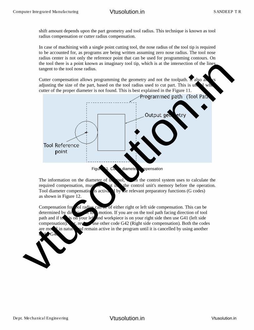
shift amount depends upon the part geometry and tool radius. This technique is known as tool radius compensation or cutter radius compensation.
In case of machining with a single point cutting tool, the nose radius of the tool tip is required to be accounted for, as programs are being written assuming zero nose radius. The tool nose radius center is not only the reference point that can be used for programming contours. On the tool there is a point known as imaginary tool tip, which is at the intersection of the lines tangent to the tool nose radius.
Cutter compensation allows programming the geometry and not the toolpath. It also allows adjusting the size of the part, based on the tool radius used to cut part. This is useful when cutter of the proper diameter is not found. This is best explained in the Figure 11.
Figure 11. Cutter diameter compensation
The information on the diameter of the tool, which the control system uses to calculate the required compensation, must be input into the control unit's memory before the operation. Tool diameter compensation is activated by the relevant preparatory functions (G codes) as shown in Figure 12.
Compensation for tool radius can be of either right or left side compensation. This can be determined by direction of tool motion. If you are on the tool path facing direction of tool path and if tool is on your left and workpiece is on your right side then use G41 (left side compensation). For, reverse use other code G42 (Right side compensation). Both the codes are modal in nature and remain active in the program until it is cancelled by using another code, G40.
Computer Integrated Manufacturing SANDEEP T R
Dept. Mechanical Engineering Vtusolution.in
Vtusolution.in
Vtusolution.in
vtuso
lution
.in
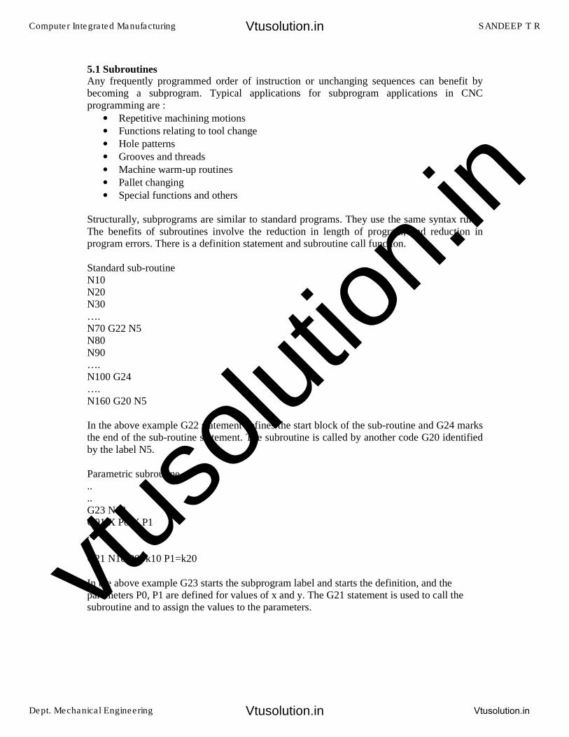
5.1 Subroutines Any frequently programmed order of instruction or unchanging sequences can benefit by becoming a subprogram. Typical applications for subprogram applications in CNC programming are :
• Repetitive machining motions
• Functions relating to tool change
• Hole patterns
• Grooves and threads
• Machine warm-up routines
• Pallet changing
• Special functions and others
Structurally, subprograms are similar to standard programs. They use the same syntax rules. The benefits of subroutines involve the reduction in length of program, and reduction in program errors. There is a definition statement and subroutine call function.
Standard sub-routine N10 N20 N30 …. N70 G22 N5 N80 N90 …. N100 G24 …. N160 G20 N5
In the above example G22 statement defines the start block of the sub-routine and G24 marks the end of the sub-routine statement. The subroutine is called by another code G20 identified by the label N5.
Parametric subroutine .. .. G23 N18 G01 X P0 Y P1 .. .. G21 N18 P0=k10 P1=k20
In the above example G23 starts the subprogram label and starts the definition, and the parameters P0, P1 are defined for values of x and y. The G21 statement is used to call the subroutine and to assign the values to the parameters.
Computer Integrated Manufacturing SANDEEP T R
Dept. Mechanical Engineering Vtusolution.in
Vtusolution.in
Vtusolution.in
vtuso
lution
.in

5.2 Canned Cycles A canned cycle is a preprogrammed sequence of events / motions of tool / spindle stored in memory of controller. Every canned cycle has a format. Canned cycle is modal in nature and remains activated until cancelled. Canned cycles are a great resource to make manual programming easier. Often underutilized, canned cycles save time and effort.
5.2.1 Machining a Rectangular pocket
This cycle assumes the cutter is initially placed over the center of the pocket and at some clearance distance (typically 0.100 inch) above the top of the pocket. Then the cycle will take over from that point, plunging the cutter down to the "peck depth" and feeding the cutter around the pocket in ever increasing increments until the final size is attained. The process is repeated until the desired total depth is attained. Then the cutter is returned to the center of the pocket at the clearance height as shown in figure 14
Figure 14. Pocket machining
The overall length and width of the pocket, rather than the distance of cutter motion, are programmed into this cycle.
The syntax is : G87 Xx Yy Zz Ii Jj Kk Bb Cc Dd Hh Ll Ss (This g code is entirely controller specific and the syntax may vary between controller to controller).
Computer Integrated Manufacturing SANDEEP T R
Dept. Mechanical Engineering Vtusolution.in
Vtusolution.in
Vtusolution.in
vtuso
lution
.in
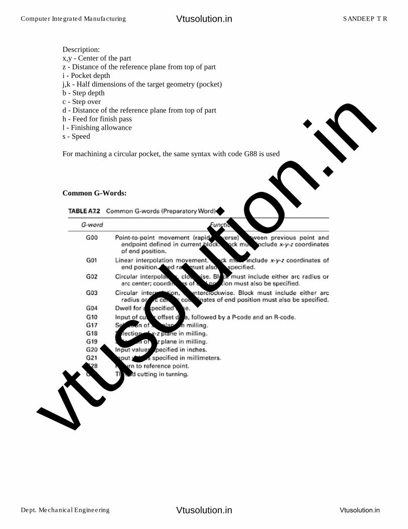
Description: x,y - Center of the part z - Distance of the reference plane from top of part i - Pocket depth j,k - Half dimensions of the target geometry (pocket) b - Step depth c - Step over d - Distance of the reference plane from top of part h - Feed for finish pass l - Finishing allowance s - Speed
For machining a circular pocket, the same syntax with code G88 is used
Common G-Words:
Computer Integrated Manufacturing SANDEEP T R
Dept. Mechanical Engineering Vtusolution.in
Vtusolution.in
Vtusolution.in
vtuso
lution
.in
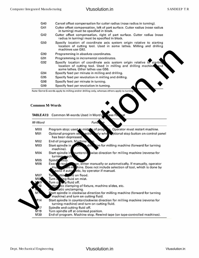
Common M-Words
Computer Integrated Manufacturing SANDEEP T R
Dept. Mechanical Engineering Vtusolution.in
Vtusolution.in
Vtusolution.in
vtuso
lution
.in
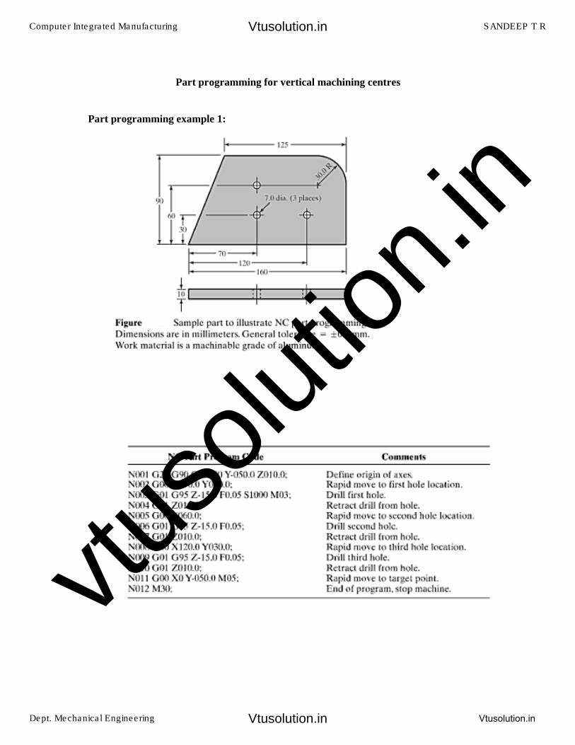
Part programming for vertical machining centres
Part programming example 1:
Computer Integrated Manufacturing SANDEEP T R
Dept. Mechanical Engineering Vtusolution.in
Vtusolution.in
Vtusolution.in
vtuso
lution
.in
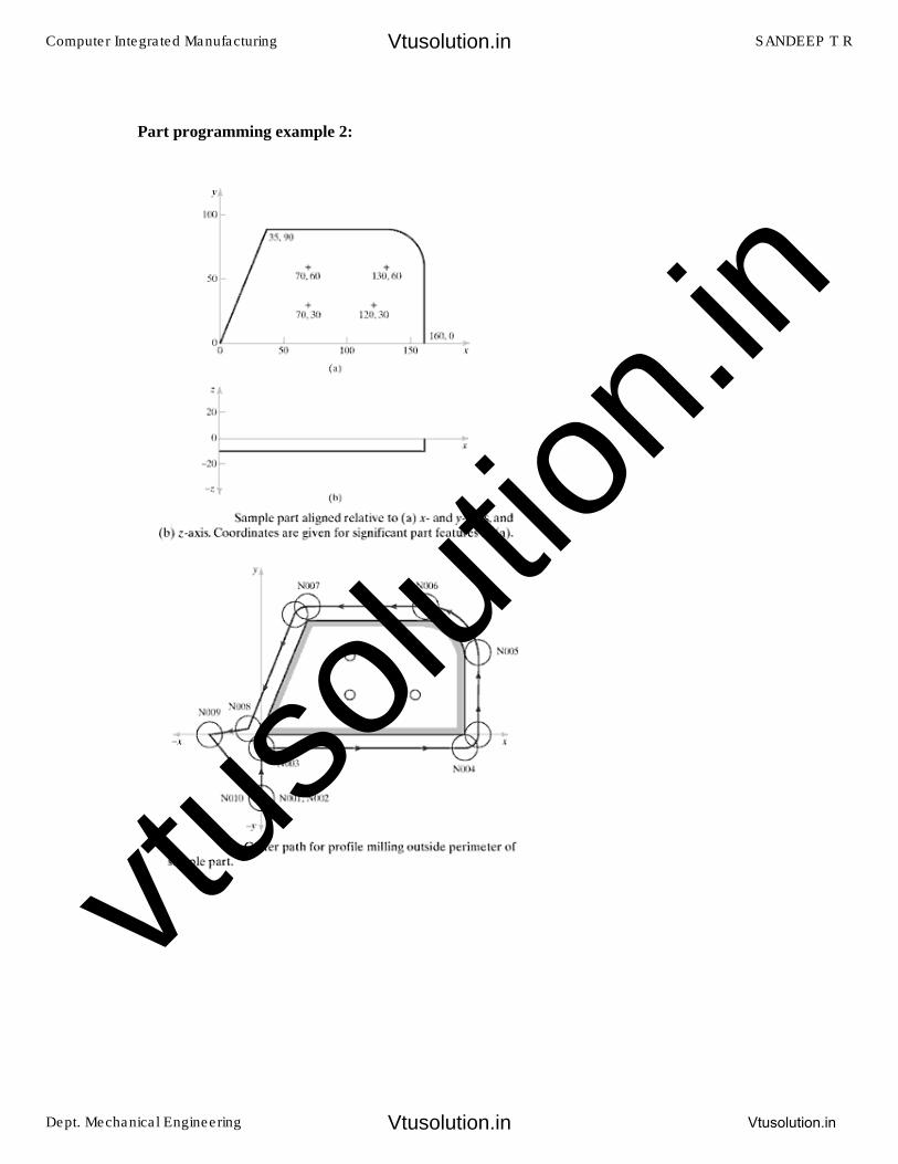
Part programming example 2:
Computer Integrated Manufacturing SANDEEP T R
Dept. Mechanical Engineering Vtusolution.in
Vtusolution.in
Vtusolution.in
vtuso
lution
.in
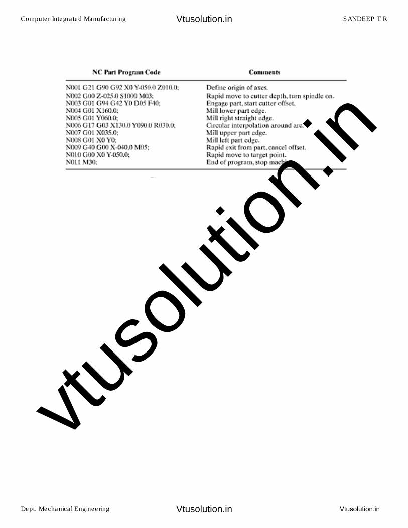
Computer Integrated Manufacturing SANDEEP T R
Dept. Mechanical Engineering Vtusolution.in
Vtusolution.in
Vtusolution.in
vtuso
lution
.in
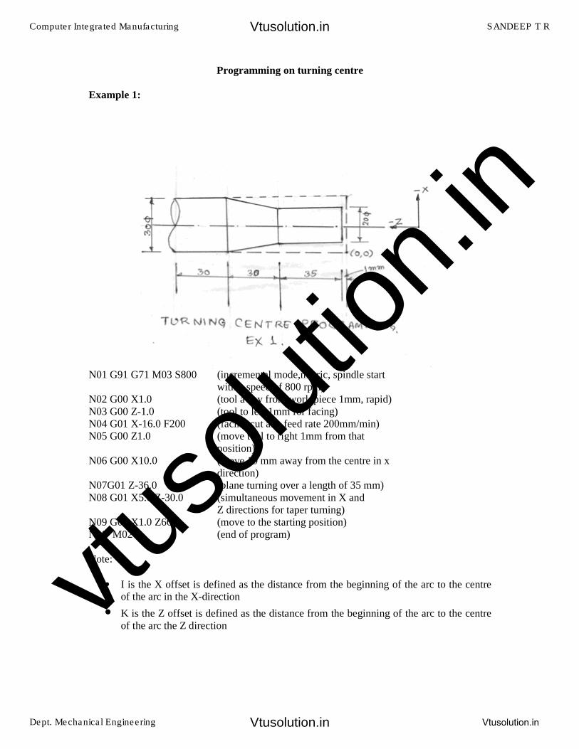
Programming on turning centre
Example 1:
N01 G91 G71 M03 S800 (incremental mode,metric, spindle start with a speed of 800 rpm)
N02 G00 X1.0 (tool away from work piece 1mm, rapid) N03 G00 Z-1.0 (tool to left 1mm for facing) N04 G01 X-16.0 F200 (facing cut at a feed rate 200mm/min) N05 G00 Z1.0 (move tool to right 1mm from that
position) N06 G00 X10.0 (move 10 mm away from the centre in x
direction) N07G01 Z-36.0 (plane turning over a length of 35 mm) N08 G01 X5.0 Z-30.0 (simultaneous movement in X and
Z directions for taper turning) N09 G00 X1.0 Z66.0 (move to the starting position) N10 M02 (end of program)
Note:
• I is the X offset is defined as the distance from the beginning of the arc to the centreof the arc in the X-direction
• K is the Z offset is defined as the distance from the beginning of the arc to the centreof the arc the Z direction
Computer Integrated Manufacturing SANDEEP T R
Dept. Mechanical Engineering Vtusolution.in
Vtusolution.in
Vtusolution.in
vtuso
lution
.in

Example 2:
N01 G90 G71 M03 S800 (absolute, metric, start spindle at a speed 800 rpm)
N02 G00 X0.0 Y0.0 (move tool to the beginning of cut) N03 G02 X10.0 Z-10.0 I 0.0 K-10.0 F150 (clockwise circular interpolation, I&K are
offsets, feed rate 150mm/min) N04 G00 Z-30.0 (move from point B to point C) N05 G03 X15.0 Z-35.0 I5.0 K0.0 (counterclockwise interpolation, I&K are
offsets, move to point D) N06 M02 (end of program)
Note:
• I is the X offset is defined as the distance from the beginning of the arc to the centreof the arc in the X-direction
• K is the Z offset is defined as the distance from the beginning of the arc to the centreof the arc the Z direction
Computer Integrated Manufacturing SANDEEP T R
Dept. Mechanical Engineering Vtusolution.in
Vtusolution.in
Vtusolution.in
vtuso
lution
.in
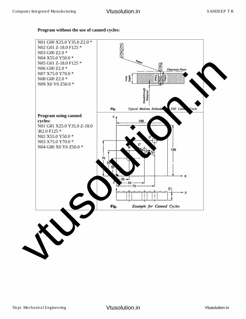
Program without the use of canned cycles:
N01 G00 X25.0 Y35.0 Z2.0 * N02 G01 Z-18.0 F125 * N03 G00 Z2.0 * N04 X55.0 Y50.0 * N05 G01 Z-18.0 F125 * N06 G00 Z2.0 * N07 X75.0 Y70.0 * N08 G00 Z2.0 * N09 X0 Y0 Z50.0 *
Program using canned
cycles:
N01 G81 X25.0 Y35.0 Z-18.0 \R2.0 F125 * N02 X55.0 Y50.0 * N03 X75.0 Y70.0 * N04 G80 X0 Y0 Z50.0 *
Computer Integrated Manufacturing SANDEEP T R
Dept. Mechanical Engineering Vtusolution.in
Vtusolution.in
Vtusolution.in
vtuso
lution
.in
PART PROGRAMMING WITH APT
APT is an acronym that stands for Automatically Programmed Tooling. It is a three dimensional NC part programming system that was developed in the late 1950s and early 1960s. Today it remains an important language in the United States and around the world, and most of the CAD/CAM approaches to part programming are based on APT. APT is also important because many of the concepts incorporated into it formed the basis for other subsequently developed systems in interactive graphics. APT was originally intended as a contouring language, but modern versions can be used for both point-to-point and contouring operations in upto five axes. Our discussion will be limited to the three linear axes, x, y and z. APT can be used for a variety of machining operations. Our coverage will concentrate on drilling (point-to-point) and milling (contouring) operations. There are more than 500 words in the APT vocabulary. Only a small (but important) fraction of the total lexicon will be covered here.
APT is not a language; it is also the computer program that processes the APT statements to calculate the corresponding cutter positions and generate the machine tool control commands. To program in APT, the programmer must first define the part geometry. Then the tool is directed to various point locations and along surfaces of the workpart to accomplish the required machining operations. The viewpoint of the programmer is that the workpiece remains stationary, and the tool is instructed to move relative to the part. To complete the program, speeds and feeds must be specific, tools must be called, tolerances must be given for circular interpolation, and so forth. Thus, there are four basic types of statements in the APT language.
1. Geometry statements are used to define the geometry elements that comprise thepart.
2. Motion commands are used to specify the tool path3. Postprocessor statements control the machine tool operation, for example, to specify
speeds and feeds, set tolerance values for circular interpolation, and actuate othercapabilities of the machine tool.
4. Auxiliary statements are a group of miscellaneous statements used to name the partprogram, insert comments in the program, and accomplish similar functions.
These statements are constructed of APT vocabulary words, symbols, and numbers, all arranged using appropriate punctuation. APT vocabulary words consist of six or fewer characters. Such a restriction seems archaic today, but it must be remembered that APT was developed in the 1950s, when computer memory technology was extremely limited. Most APT statements include a slash (/) as part of the punctuation. APT vocabulary words that immediately precede the slash are called major words, whereas those that follow the slash are called minor words.
Computer Integrated Manufacturing SANDEEP T R
Dept. Mechanical Engineering Vtusolution.in
Vtusolution.in
Vtusolution.in
vtuso
lution
.in
APT Geometry Statements
The geometry of the part must be defined to identify the surfaces and features that are to be machined. Accordingly, the points, lines, and surfaces must be defined in the program prior to specifying the motion statements. The general form of an APT geometry statements is the following:
SYMBOL = GEOMETRY TYPE/descriptive data
An example of such a statement is
P1 = POINT/20.0, 40.0, 60.0
An APT geometry statement consists of three sections. The first is the symbol used to identify the geometry element. A symbol can be any combination of six or fewer alphabetical and numerical characters, at least one of which must be alphabetical. Also, the symbol cannot be an APT vocabulary word. The second section of the APT geometry statement is an APT major word that identifies the type of geometry element. Examples are POINT, LINE, CIRCLE and PLANE. The third section of the APT geometry statement provides the descriptive data that define the element precisely, completely, and uniquely. These data may include numerical values to specify dimensional and position data, previously defined geometry elements, and APT minor words. Punctuation in an APT geometry statement is indicated in the preceding geometry statements. The geometry definition is written as an equation, the symbol being equated to the element type, followed by a slash with descriptive data to the right of the slash. Commas are used to separate the words and numerical values in the descriptive data. There are a variety of ways to specify geometry elements. In the following discussion, examples of APT statements will be presented for points, lines, planes, and circles.
Points :
Specification of a point is most easily accomplished by designating its x-,y-, and z-coordinates.
P1 = POINT/20.0, 40.0, 60.0
where the descriptive data following the slash indicate x-,y-, and z-coordinates. The specification can be done in either inches or millimeters (metric). We use metric values in our examples. As an alternative, a point can be defined as the intersection of two intersecting lines, as in the following:
P1 = POINT/INTOF, L1, L2
where the APT word INTOF in the descriptive data stands for “intersection of”.
Other methods of defining points are also available. Several are illustrated in Figure 1. The associated points are identified in the following APT statements:
Computer Integrated Manufacturing SANDEEP T R
Dept. Mechanical Engineering Vtusolution.in
Vtusolution.in
Vtusolution.in
vtuso
lution
.in
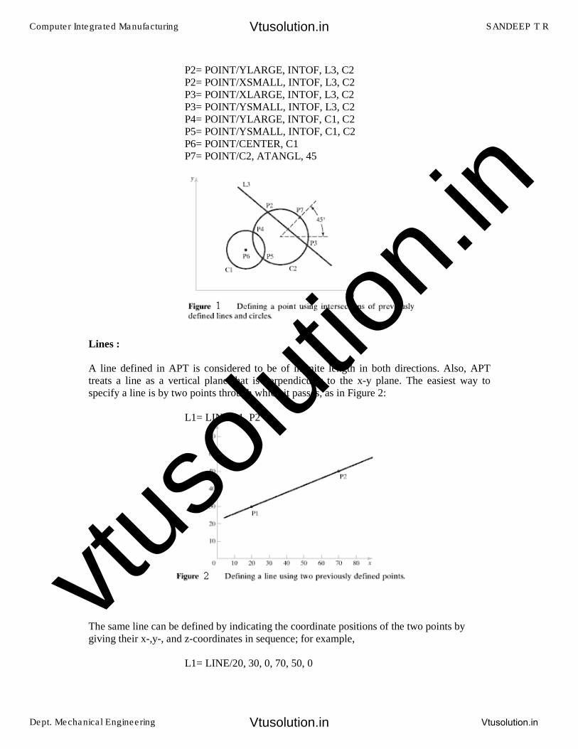
P2= POINT/YLARGE, INTOF, L3, C2 P2= POINT/XSMALL, INTOF, L3, C2 P3= POINT/XLARGE, INTOF, L3, C2 P3= POINT/YSMALL, INTOF, L3, C2 P4= POINT/YLARGE, INTOF, C1, C2 P5= POINT/YSMALL, INTOF, C1, C2 P6= POINT/CENTER, C1 P7= POINT/C2, ATANGL, 45
Lines :
A line defined in APT is considered to be of infinite length in both directions. Also, APT treats a line as a vertical plane that is perpendicular to the x-y plane. The easiest way to specify a line is by two points through which it passes, as in Figure 2:
L1= LINE/P1, P2
The same line can be defined by indicating the coordinate positions of the two points by giving their x-,y-, and z-coordinates in sequence; for example,
L1= LINE/20, 30, 0, 70, 50, 0
Computer Integrated Manufacturing SANDEEP T R
Dept. Mechanical Engineering Vtusolution.in
Vtusolution.in
Vtusolution.in
vtuso
lution
.in
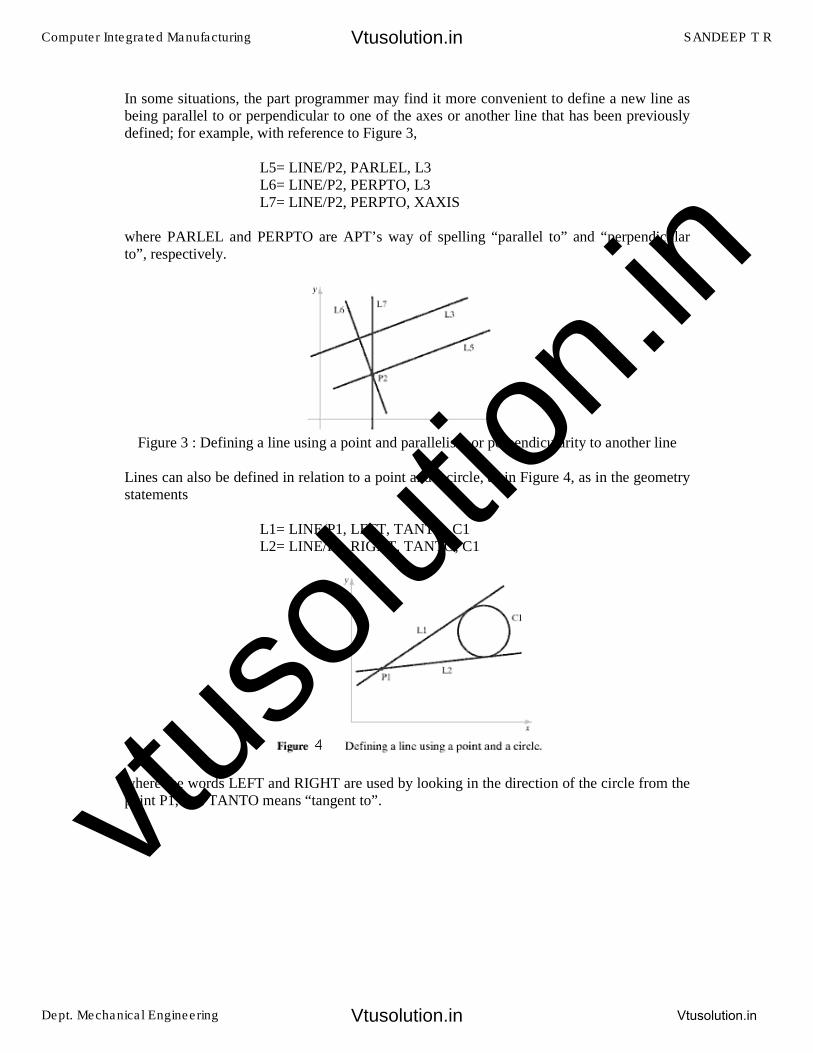
In some situations, the part programmer may find it more convenient to define a new line as being parallel to or perpendicular to one of the axes or another line that has been previously defined; for example, with reference to Figure 3,
L5= LINE/P2, PARLEL, L3 L6= LINE/P2, PERPTO, L3 L7= LINE/P2, PERPTO, XAXIS
where PARLEL and PERPTO are APT’s way of spelling “parallel to” and “perpendicular to”, respectively.
Figure 3 : Defining a line using a point and parallelism or perpendicularity to another line
Lines can also be defined in relation to a point and a circle, as in Figure 4, as in the geometry statements
L1= LINE/P1, LEFT, TANTO, C1 L2= LINE/P1, RIGHT, TANTO, C1
where the words LEFT and RIGHT are used by looking in the direction of the circle from the point P1, and TANTO means “tangent to”.
Computer Integrated Manufacturing SANDEEP T R
Dept. Mechanical Engineering Vtusolution.in
Vtusolution.in
Vtusolution.in
vtuso
lution
.in
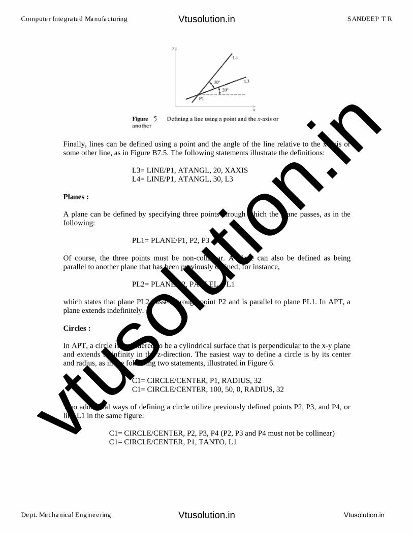
Finally, lines can be defined using a point and the angle of the line relative to the x-axis or some other line, as in Figure B7.5. The following statements illustrate the definitions:
L3= LINE/P1, ATANGL, 20, XAXIS L4= LINE/P1, ATANGL, 30, L3
Planes :
A plane can be defined by specifying three points through which the plane passes, as in the following:
PL1= PLANE/P1, P2, P3
Of course, the three points must be non-collinear. A plane can also be defined as being parallel to another plane that has been previously defined; for instance,
PL2= PLANE/P2, PARLEL, PL1
which states that plane PL2 passes through point P2 and is parallel to plane PL1. In APT, a plane extends indefinitely.
Circles :
In APT, a circle is considered to be a cylindrical surface that is perpendicular to the x-y plane and extends to infinity in the z-direction. The easiest way to define a circle is by its center and radius, as in the following two statements, illustrated in Figure 6.
C1= CIRCLE/CENTER, P1, RADIUS, 32 C1= CIRCLE/CENTER, 100, 50, 0, RADIUS, 32
Two additional ways of defining a circle utilize previously defined points P2, P3, and P4, or line L1 in the same figure:
C1= CIRCLE/CENTER, P2, P3, P4 (P2, P3 and P4 must not be collinear) C1= CIRCLE/CENTER, P1, TANTO, L1
Computer Integrated Manufacturing SANDEEP T R
Dept. Mechanical Engineering Vtusolution.in
Vtusolution.in
Vtusolution.in
vtuso
lution
.in
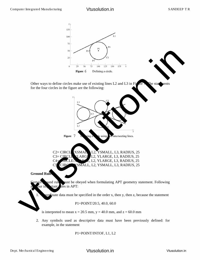
Other ways to define circles make use of existing lines L2 and L3 in Figure 7. The statements for the four circles in the figure are the following:
C2= CIRCLE/XSMALL, L2, YSMALL, L3, RADIUS, 25 C3= CIRCLE/YLARGE, L2, YLARGE, L3, RADIUS, 25 C4= CIRCLE/XLARGE, L2, YLARGE, L3, RADIUS, 25 C5= CIRCLE/YSMALL, L2, YSMALL, L3, RADIUS, 25
Ground Rules :
Certain ground rules must be obeyed when formulating APT geometry statement. Following are four important rules in APT:
1. Coordinate data must be specified in the order x, then y, then z, because the statement
P1=POINT/20.5, 40.0, 60.0
is interpreted to mean x = 20.5 mm, y = 40.0 mm, and z = 60.0 mm
2. Any symbols used as descriptive data must have been previously defined: forexample, in the statement
P1=POINT/INTOF, L1, L2
Computer Integrated Manufacturing SANDEEP T R
Dept. Mechanical Engineering Vtusolution.in
Vtusolution.in
Vtusolution.in
vtuso
lution
.in
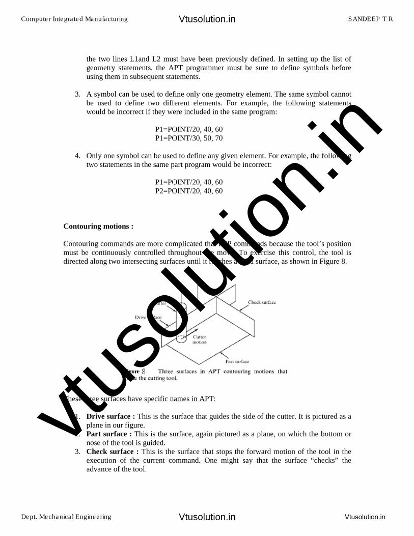
the two lines L1and L2 must have been previously defined. In setting up the list of geometry statements, the APT programmer must be sure to define symbols before using them in subsequent statements.
3. A symbol can be used to define only one geometry element. The same symbol cannotbe used to define two different elements. For example, the following statementswould be incorrect if they were included in the same program:
P1=POINT/20, 40, 60 P1=POINT/30, 50, 70
4. Only one symbol can be used to define any given element. For example, the followingtwo statements in the same part program would be incorrect:
P1=POINT/20, 40, 60 P2=POINT/20, 40, 60
Contouring motions :
Contouring commands are more complicated that PTP commands because the tool’s position must be continuously controlled throughout the move. To exercise this control, the tool is directed along two intersecting surfaces until it reaches a third surface, as shown in Figure 8.
These three surfaces have specific names in APT:
1. Drive surface : This is the surface that guides the side of the cutter. It is pictured as aplane in our figure.
2. Part surface : This is the surface, again pictured as a plane, on which the bottom ornose of the tool is guided.
3. Check surface : This is the surface that stops the forward motion of the tool in theexecution of the current command. One might say that the surface “checks” theadvance of the tool.
Computer Integrated Manufacturing SANDEEP T R
Dept. Mechanical Engineering Vtusolution.in
Vtusolution.in
Vtusolution.in
vtuso
lution
.in
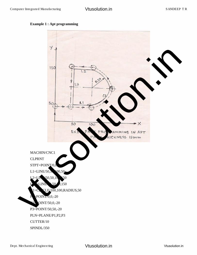
Example 1 : Apt programming
MACHIN/CNC1
CLPRNT
STPT=POINT/0,0
L1=LINE/50,50,100,50
L2=LINE/50,50,100,150
L3==LINE/50,50,50,150
C1=CIRCLE/100,100,RADIUS,50
P1=POINT/0,0,-20
P2=POINT/50,0,-20
P3=POINT/50,50,-20
PLN=PLANE/P1,P2,P3
CUTTER/10
SPINDL/350
Computer Integrated Manufacturing SANDEEP T R
Dept. Mechanical Engineering Vtusolution.in
Vtusolution.in
Vtusolution.in
vtuso
lution
.in
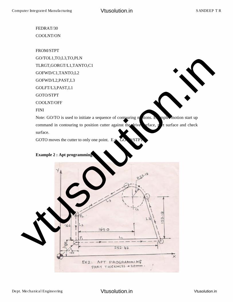
FEDRAT/30
COOLNT/ON
FROM/STPT
GO/TOL1,TO,L3,TO,PLN
TLRGT,GORGT/L1,TANTO,C1
GOFWD/C1,TANTO,L2
GOFWD/L2,PAST,L3
GOLFT/L3,PAST,L1
GOTO/STPT
COOLNT/OFF
FINI
Note: GO/TO is used to initiate a sequence of contouring motions. Example: motion start up
command in contouring to position cutter against the drive surface, part surface and check
surface.
GOTO moves the cutter to only one point. E.g. GOTO/STPT
Example 2 : Apt programming
Computer Integrated Manufacturing SANDEEP T R
Dept. Mechanical Engineering Vtusolution.in
Vtusolution.in
Vtusolution.in
vtuso
lution
.in
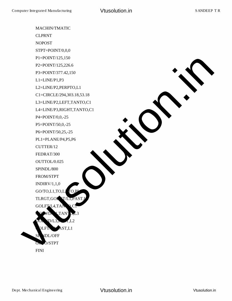
MACHIN/TMATIC
CLPRNT
NOPOST
STPT=POINT/0,0,0
P1=POINT/125,150
P2=POINT/125,226.6
P3=POINT/377.42,150
L1=LINE/P1,P3
L2=LINE/P2,PERPTO,L1
C1=CIRCLE/294,303.18,53.18
L3=LINE/P2,LEFT,TANTO,C1
L4=LINE/P3,RIGHT,TANTO,C1
P4=POINT/0,0,-25
P5=POINT/50,0,-25
P6=POINT/50,25,-25
PL1=PLANE/P4,P5,P6
CUTTER/12
FEDRAT/300
OUTTOL/0.025
SPINDL/800
FROM/STPT
INDIRV/1,1,0
GO/TO,L1,TO,L2,TO,PL1
TLRGT,GORGT/L1,PAST,L4
GOLFT/L4,TANTO,C1
GOFWD/C1,TANTO,L3
GOFWD/L3,PAST,L2
GOLFT/L2,PAST,L1
SPINDL/OFF
GOTO/STPT
FINI
Computer Integrated Manufacturing SANDEEP T R
Dept. Mechanical Engineering Vtusolution.in
Vtusolution.in
Vtusolution.in
vtuso
lution
.in
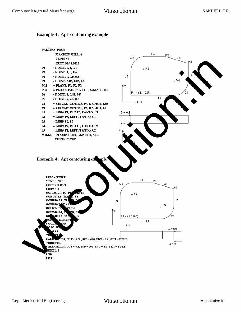
Example 3 : Apt contouring example
Example 4 : Apt contouring example
Computer Integrated Manufacturing SANDEEP T R
Dept. Mechanical Engineering Vtusolution.in
Vtusolution.in
Vtusolution.in
vtuso
lution
.in
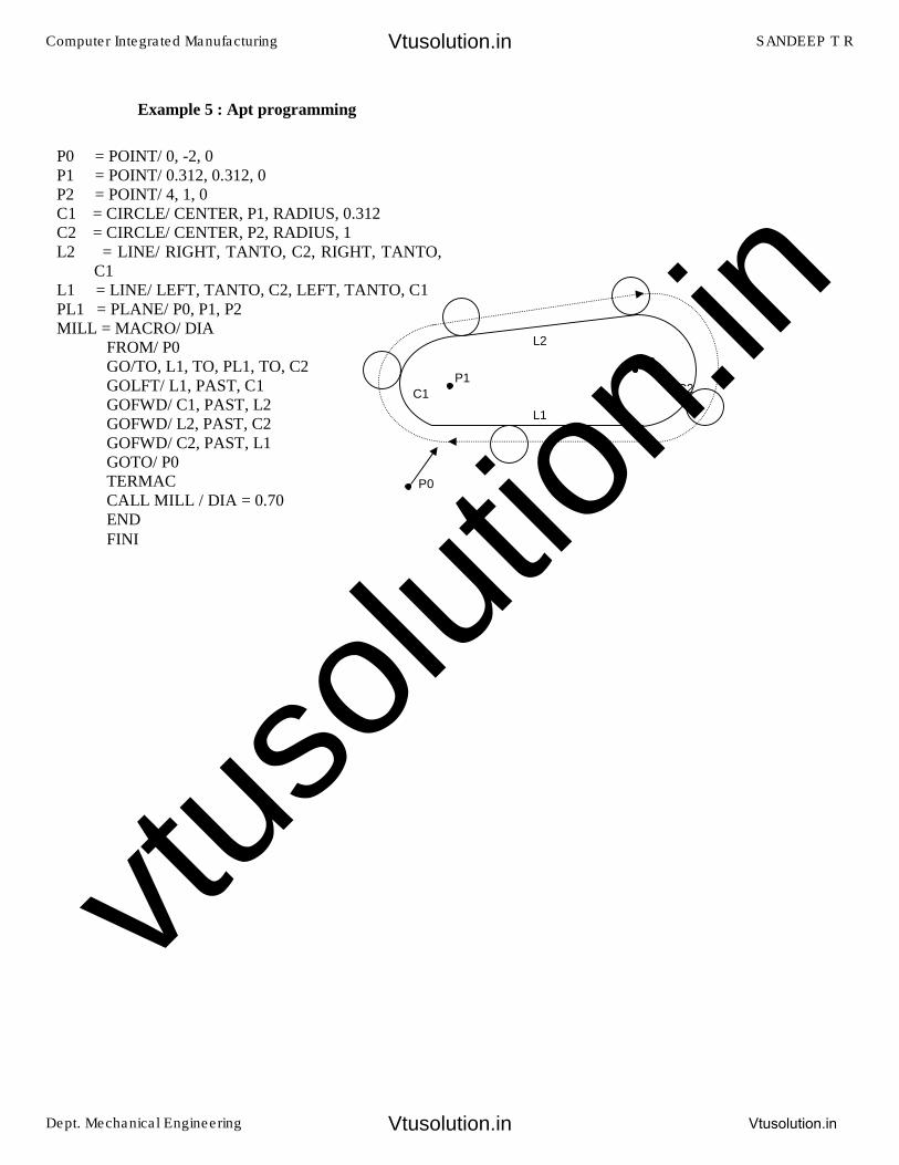
Example 5 : Apt programming
P0 = POINT/ 0, -2, 0 P1 = POINT/ 0.312, 0.312, 0 P2 = POINT/ 4, 1, 0 C1 = CIRCLE/ CENTER, P1, RADIUS, 0.312 C2 = CIRCLE/ CENTER, P2, RADIUS, 1 L2 = LINE/ RIGHT, TANTO, C2, RIGHT, TANTO,
C1 L1 = LINE/ LEFT, TANTO, C2, LEFT, TANTO, C1 PL1 = PLANE/ P0, P1, P2 MILL = MACRO/ DIA
FROM/ P0 GO/TO, L1, TO, PL1, TO, C2 GOLFT/ L1, PAST, C1 GOFWD/ C1, PAST, L2 GOFWD/ L2, PAST, C2 GOFWD/ C2, PAST, L1 GOTO/ P0 TERMAC CALL MILL / DIA = 0.70 END
FINI
P1
P2
L2
L1
C1 C2
P0
Computer Integrated Manufacturing SANDEEP T R
Dept. Mechanical Engineering Vtusolution.in
Vtusolution.in
Vtusolution.in
vtuso
lution
.in
Unit 8 :
ROBOTICS
INTRODUCTION
Robots are devices that are programmed to move parts, or to do work with a tool. Robotics is a multidisciplinary engineering field dedicated to the development of autonomous devices, including manipulators and mobile vehicles.
The Origins of Robots
Year 1250
Bishop Albertus Magnus holds banquet at which guests were served by metal attendants. Upon seeing this, Saint Thomas Aquinas smashed the attendants to bits and called the bishop a sorcerer.
Year 1640
Descartes builds a female automaton which he calls “Ma fille Francine.” She accompanied
Descartes on a voyage and was thrown overboard by the captain, who thought she was the
work of Satan.
Year 1738
Jacques de Vaucanson builds a mechanical duck quack, bathe, drink water, eat grain, digest it and void it. Whereabouts of the duck are unknown today.
Year 1805
Doll, made by Maillardet, that wrote in either French or English and could draw landscapes
Year 1923
Karel Capek coins the term robot in his play Rossum’s Universal Robots (R.U.R). Robot comes from the Czech word robota , which means “servitude, forced labor.”
Year 1940
Sparko, the Westinghouse dog, was developed which used both mechanical and electrical components.
Computer Integrated Manufacturing SANDEEP T R
Dept. Mechanical Engineering Vtusolution.in
Vtusolution.in
Vtusolution.in
vtuso
lution
.in
Year 1950’s to 1960’s
Computer technology advances and control machinery is developed. Questions Arise: Is the computer an immobile robot? Industrial Robots created. Robotic Industries Association states that an “industrial robot is a re-programmable, multifunctional manipulator designed to move materials, parts, tools, or specialized devices through variable programmed motions to perform a variety of tasks”
Year 1956
Researchers aim to combine “perceptual and problem-solving capabilities,” using computers, cameras, and touch sensors. The idea is to study the types of intelligent actions these robots are capable of. A new discipline is born: A.I.
Year 1960
Shakey is made at Stanford Research Institute International. It contained a television camera, range finder, on-board logic, bump sensors, camera control unit, and an antenna for a radio link. Shakey was controlled by a computer in a different room.
The first industrial robot: UNIMATE Year 1954
The first programmable robot is designed by George Devol, who coins the term Universal Automation. He later shortens this to Unimation, which becomes the name of the first robot company (1962).
Year 1978
The Puma (Programmable Universal Machine for Assembly) robot is developed by Unimation with a General Motors design support
Year 1980s
The robot industry enters a phase of rapid growth. Many institutions introduce programs and courses in robotics. Robotics courses are spread across mechanical engineering, electrical engineering, and computer science departments.
Year 1995-present
Emerging applications in small robotics and mobile robots drive a second
growth of start-up companies and research
2003
NASA’s Mars Exploration Rovers will launch toward Mars in search of answers about the history of water on Mars
Computer Integrated Manufacturing SANDEEP T R
Dept. Mechanical Engineering Vtusolution.in
Vtusolution.in
Vtusolution.in
vtuso
lution
.in
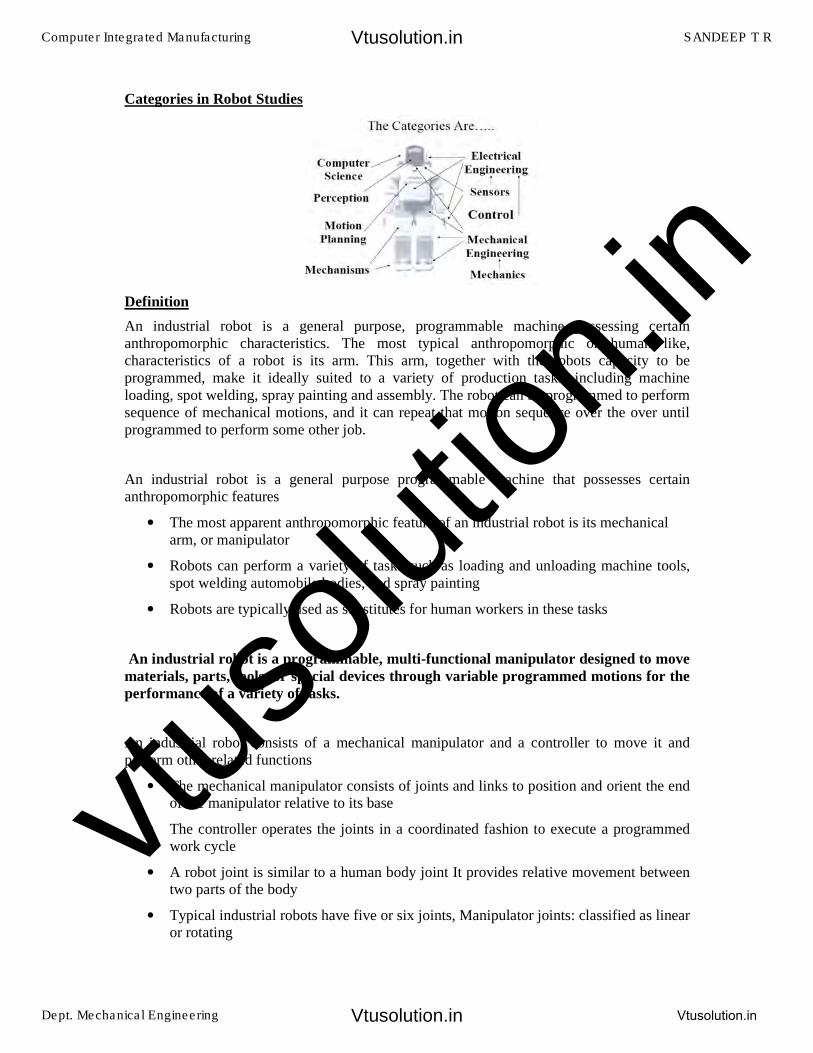
Categories in Robot Studies
Definition
An industrial robot is a general purpose, programmable machine possessing certain anthropomorphic characteristics. The most typical anthropomorphic or human like, characteristics of a robot is its arm. This arm, together with the robots capacity to be programmed, make it ideally suited to a variety of production tasks, including machine loading, spot welding, spray painting and assembly. The robot can be programmed to perform sequence of mechanical motions, and it can repeat that motion sequence over the over until programmed to perform some other job.
An industrial robot is a general purpose programmable machine that possesses certain anthropomorphic features
• The most apparent anthropomorphic feature of an industrial robot is its mechanicalarm, or manipulator
• Robots can perform a variety of tasks such as loading and unloading machine tools,spot welding automobile bodies, and spray painting
• Robots are typically used as substitutes for human workers in these tasks
An industrial robot is a programmable, multi-functional manipulator designed to move
materials, parts, tools, or special devices through variable programmed motions for the
performance of a variety of tasks.
An industrial robot consists of a mechanical manipulator and a controller to move it and perform other related functions
• The mechanical manipulator consists of joints and links to position and orient the endof the manipulator relative to its base
• The controller operates the joints in a coordinated fashion to execute a programmedwork cycle
• A robot joint is similar to a human body joint It provides relative movement betweentwo parts of the body
• Typical industrial robots have five or six joints, Manipulator joints: classified as linearor rotating
Computer Integrated Manufacturing SANDEEP T R
Dept. Mechanical Engineering Vtusolution.in
Vtusolution.in
Vtusolution.in
vtuso
lution
.in
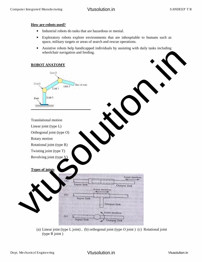
How are robots used?
• Industrial robots do tasks that are hazardous or menial.
• Exploratory robots explore environments that are inhospitable to humans such asspace, military targets or areas of search and rescue operations.
• Assistive robots help handicapped individuals by assisting with daily tasks includingwheelchair navigation and feeding.
ROBOT ANATOMY
Translational motion
Linear joint (type L)
Orthogonal joint (type O)
Rotary motion
Rotational joint (type R)
Twisting joint (type T)
Revolving joint (type V)
Types of joints
(a) Linear joint (type L joint) , (b) orthogonal joint (type O joint ) (c) Rotational joint(type R joint )
Computer Integrated Manufacturing SANDEEP T R
Dept. Mechanical Engineering Vtusolution.in
Vtusolution.in
Vtusolution.in
vtuso
lution
.in
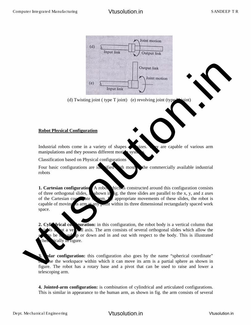
(d) Twisting joint ( type T joint) (e) revolving joint (type V joint)
Robot Physical Configuration
Industrial robots come in a variety of shapes and sizes. They are capable of various arm manipulations and they possess different motion systems.
Classification based on Physical configurations
Four basic configurations are identified with most of the commercially available industrial robots
1. Cartesian configuration: A robot which is constructed around this configuration consistsof three orthogonal slides, as shown in fig. the three slides are parallel to the x, y, and z axesof the Cartesian coordinate system. By appropriate movements of these slides, the robot iscapable of moving its arm at any point within its three dimensional rectangularly spaced workspace.
2. Cylindrical configuration: in this configuration, the robot body is a vertical column thatswivels about a vertical axis. The arm consists of several orthogonal slides which allow thearm to be moved up or down and in and out with respect to the body. This is illustratedschematically in figure.
3. Polar configuration: this configuration also goes by the name “spherical coordinate”because the workspace within which it can move its arm is a partial sphere as shown infigure. The robot has a rotary base and a pivot that can be used to raise and lower atelescoping arm.
4. Jointed-arm configuration: is combination of cylindrical and articulated configurations.This is similar in appearance to the human arm, as shown in fig. the arm consists of several
Computer Integrated Manufacturing SANDEEP T R
Dept. Mechanical Engineering Vtusolution.in
Vtusolution.in
Vtusolution.in
vtuso
lution
.in
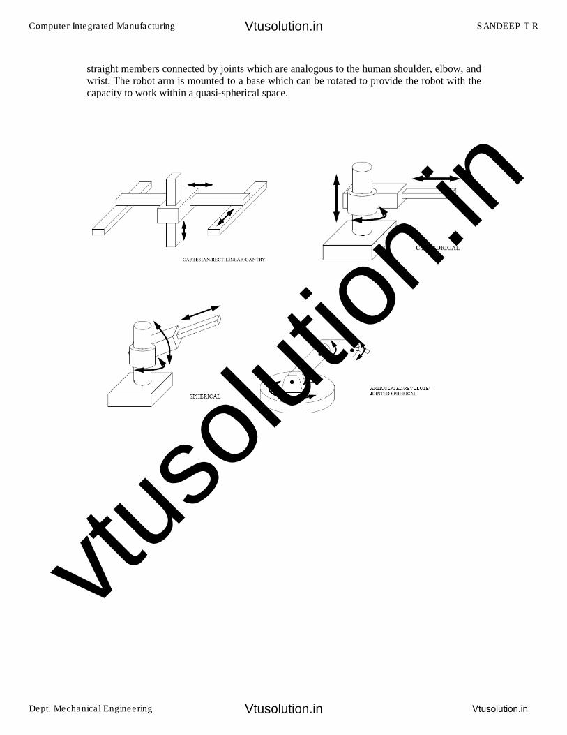
straight members connected by joints which are analogous to the human shoulder, elbow, and wrist. The robot arm is mounted to a base which can be rotated to provide the robot with the capacity to work within a quasi-spherical space.
Computer Integrated Manufacturing SANDEEP T R
Dept. Mechanical Engineering Vtusolution.in
Vtusolution.in
Vtusolution.in
vtuso
lution
.in
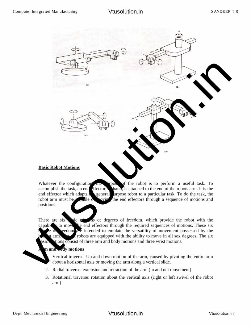
Basic Robot Motions
Whatever the configuration, the purpose of the robot is to perform a useful task. To accomplish the task, an end effector, or hand, is attached to the end of the robots arm. It is the end effector which adapts the general purpose robot to a particular task. To do the task, the robot arm must be capable of moving the end effectors through a sequence of motions and positions.
There are six basic motions or degrees of freedom, which provide the robot with the capability to move the end effectors through the required sequences of motions. These six degree of freedom are intended to emulate the versatility of movement possessed by the human arm. Not all robots are equipped with the ability to move in all sex degrees. The six basic motions consist of three arm and body motions and three wrist motions.
Arm and body motions
1. Vertical traverse: Up and down motion of the arm, caused by pivoting the entire armabout a horizontal axis or moving the arm along a vertical slide.
2. Radial traverse: extension and retraction of the arm (in and out movement)
3. Rotational traverse: rotation about the vertical axis (right or left swivel of the robotarm)
Computer Integrated Manufacturing SANDEEP T R
Dept. Mechanical Engineering Vtusolution.in
Vtusolution.in
Vtusolution.in
vtuso
lution
.in

Wrist Motion
• Wrist swivel: Rotation of the wrist
• Wrist bend: Up or down movement of the wrist, this also involves rotationmovement.
• Wrist yaw: Right or left swivel of the wrist.
Advantages and disadvantages of 5 types of robots
Configurations Advantages Disadvantages
Cartesian coordinates 3 linear axes, easy to visualize,rigid structure ,easy programming
Can only reach front of itself, requirse long room space.
Cylindrical coordinates
2 linear axes +1 rotating can reach all around itself ,reach and height axes rigid
,rotational axis easy to seal
Can’t reach above itself, base rotation axis as less rigid, linear axis
is hard to seal.
SCARA coordinates 1 linear + 2 rotational axes is rigid, large work space area for floor space
2 ways to reach point ,difficult to program offline, highly complex
arm
Spherical coordinates 1 linear + 2 rotational axes , long horizontal reach
Can’t reach around obstacles .short vertical length
Revolve coordinates 3 rotational axes can reach above or below obstacles.
Difficult to program off-line , most complex manipulator
Computer Integrated Manufacturing SANDEEP T R
Dept. Mechanical Engineering Vtusolution.in
Vtusolution.in
Vtusolution.in
vtuso
lution
.in
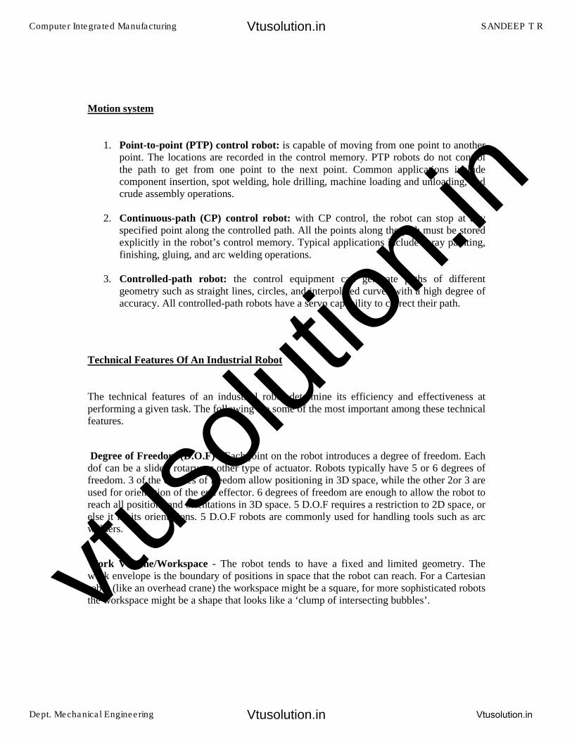
Motion system
1. Point-to-point (PTP) control robot: is capable of moving from one point to anotherpoint. The locations are recorded in the control memory. PTP robots do not controlthe path to get from one point to the next point. Common applications includecomponent insertion, spot welding, hole drilling, machine loading and unloading, andcrude assembly operations.
2. Continuous-path (CP) control robot: with CP control, the robot can stop at anyspecified point along the controlled path. All the points along the path must be storedexplicitly in the robot’s control memory. Typical applications include spray painting,finishing, gluing, and arc welding operations.
3. Controlled-path robot: the control equipment can generate paths of differentgeometry such as straight lines, circles, and interpolated curves with a high degree ofaccuracy. All controlled-path robots have a servo capability to correct their path.
Technical Features Of An Industrial Robot
The technical features of an industrial robot determine its efficiency and effectiveness at performing a given task. The following are some of the most important among these technical features.
Degree of Freedom (D.O.F) - Each joint on the robot introduces a degree of freedom. Each dof can be a slider, rotary, or other type of actuator. Robots typically have 5 or 6 degrees of freedom. 3 of the degrees of freedom allow positioning in 3D space, while the other 2or 3 are used for orientation of the end effector. 6 degrees of freedom are enough to allow the robot to reach all positions and orientations in 3D space. 5 D.O.F requires a restriction to 2D space, or else it limits orientations. 5 D.O.F robots are commonly used for handling tools such as arc welders.
Work Volume/Workspace - The robot tends to have a fixed and limited geometry. The work envelope is the boundary of positions in space that the robot can reach. For a Cartesian robot (like an overhead crane) the workspace might be a square, for more sophisticated robots the workspace might be a shape that looks like a ‘clump of intersecting bubbles’.
Computer Integrated Manufacturing SANDEEP T R
Dept. Mechanical Engineering Vtusolution.in
Vtusolution.in
Vtusolution.in
vtuso
lution
.in
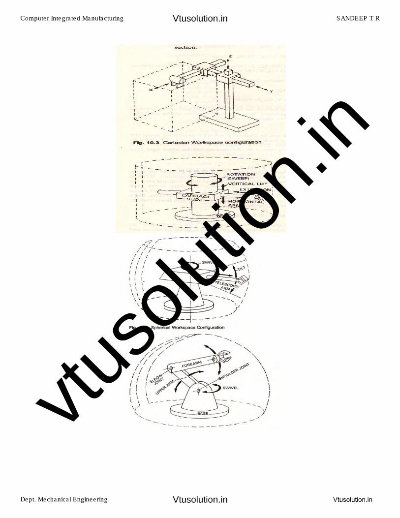
Computer Integrated Manufacturing SANDEEP T R
Dept. Mechanical Engineering Vtusolution.in
Vtusolution.in
Vtusolution.in
vtuso
lution
.in
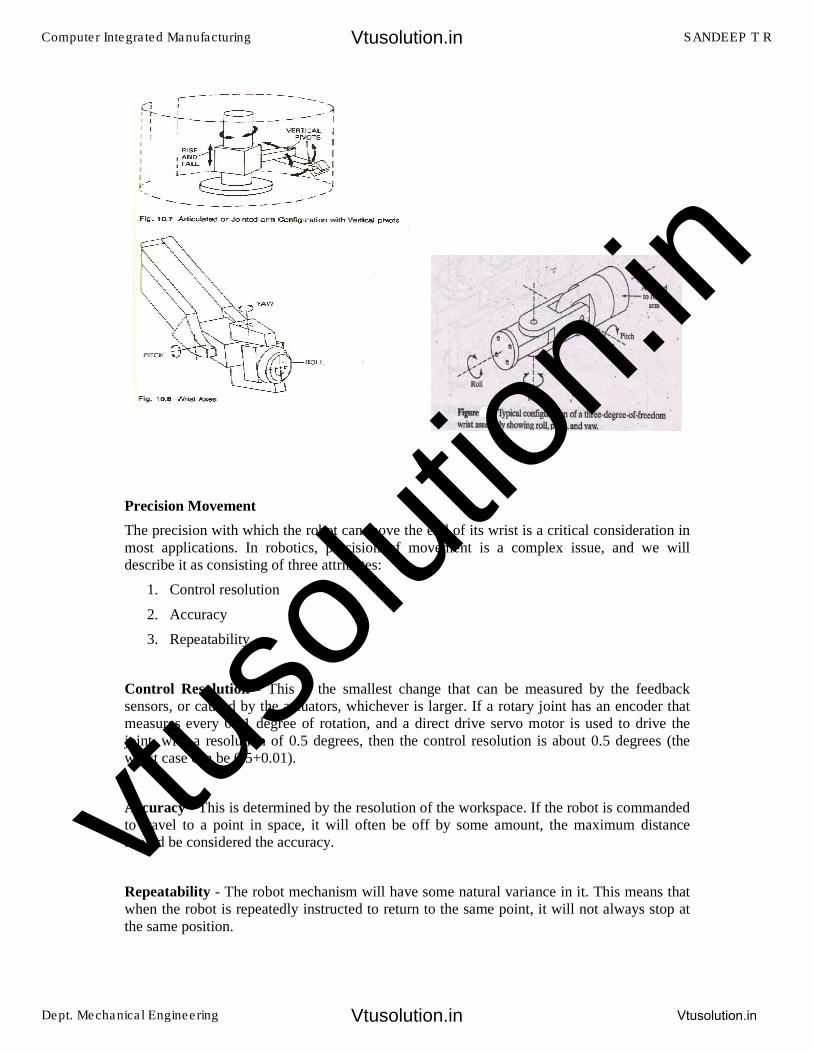
Precision Movement
The precision with which the robot can move the end of its wrist is a critical consideration in most applications. In robotics, precision of movement is a complex issue, and we will describe it as consisting of three attributes:
1. Control resolution
2. Accuracy
3. Repeatability
Control Resolution - This is the smallest change that can be measured by the feedback sensors, or caused by the actuators, whichever is larger. If a rotary joint has an encoder that measures every 0.01 degree of rotation, and a direct drive servo motor is used to drive the joint, with a resolution of 0.5 degrees, then the control resolution is about 0.5 degrees (the worst case can be 0.5+0.01).
Accuracy - This is determined by the resolution of the workspace. If the robot is commanded to travel to a point in space, it will often be off by some amount, the maximum distance should be considered the accuracy.
Repeatability - The robot mechanism will have some natural variance in it. This means that when the robot is repeatedly instructed to return to the same point, it will not always stop at the same position.
Computer Integrated Manufacturing SANDEEP T R
Dept. Mechanical Engineering Vtusolution.in
Vtusolution.in
Vtusolution.in
vtuso
lution
.in
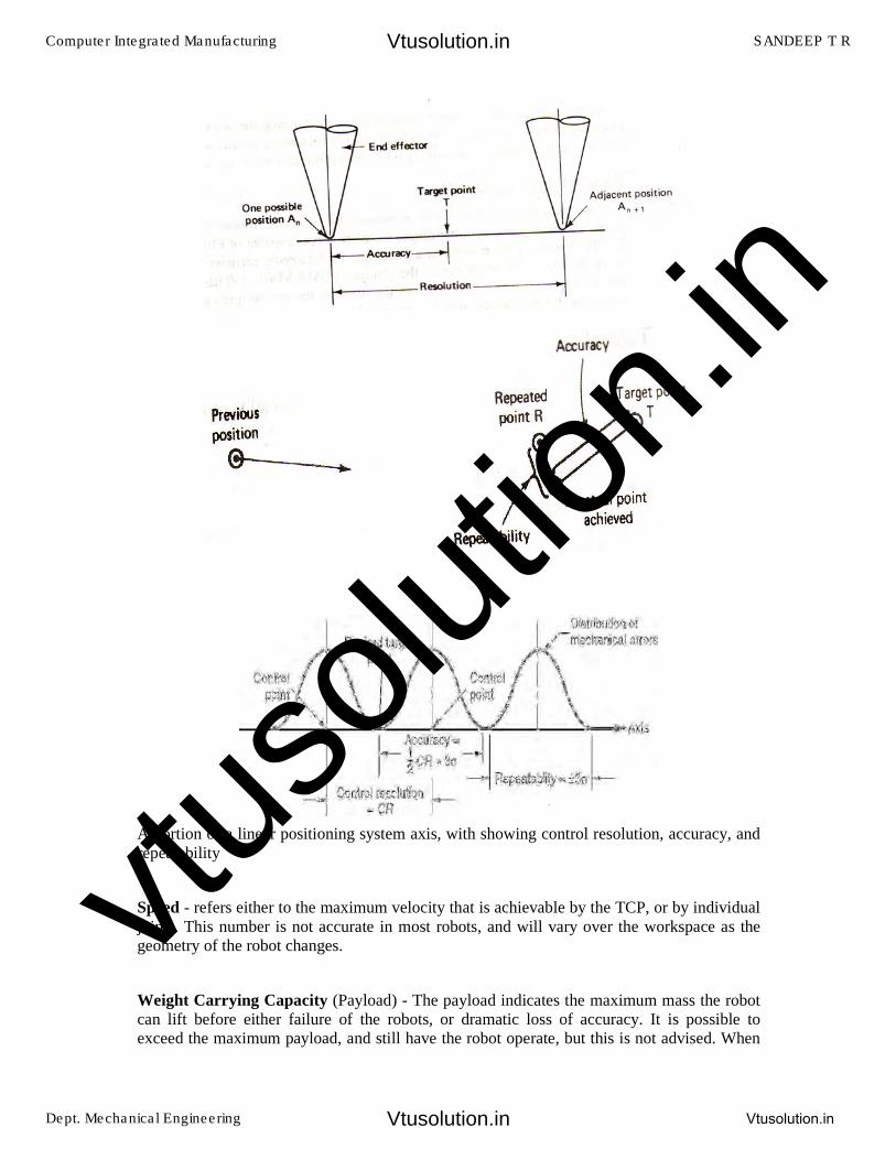
A portion of a linear positioning system axis, with showing control resolution, accuracy, and repeatability
Speed - refers either to the maximum velocity that is achievable by the TCP, or by individual joints. This number is not accurate in most robots, and will vary over the workspace as the geometry of the robot changes.
Weight Carrying Capacity (Payload) - The payload indicates the maximum mass the robot can lift before either failure of the robots, or dramatic loss of accuracy. It is possible to exceed the maximum payload, and still have the robot operate, but this is not advised. When
Computer Integrated Manufacturing SANDEEP T R
Dept. Mechanical Engineering Vtusolution.in
Vtusolution.in
Vtusolution.in
vtuso
lution
.in
the robot is accelerating fast, the payload should be less than the maximum mass. This is affected by the ability to firmly grip the part, as well as the robot structure, and the actuators. The end of arm tooling should be considered part of the payload.
Types Of Drive Systems
There are three basic drive system used in commercially available robots:
1. Hydraulic drive: gives a robot great speed and strength. These systems can be designed toactuate linear or rotational joints. The main disadvantage of a hydraulic system is that itoccupies floor space in addition to that required by the robot.
2. Electric drive: compared with a hydraulic system, an electric system provides a robot withless speed and strength. Accordingly, electric drive systems are adopted for smaller robots.However, robots supported by electric drive systems are more accurate, exhibit betterrepeatability, and are cleaner to use.
3. Pneumatic drive: are generally used for smaller robots. These robots, with fewer degreesof freedom, carry out simple pick-and-place material handling operations.
Computer Integrated Manufacturing SANDEEP T R
Dept. Mechanical Engineering Vtusolution.in
Vtusolution.in
Vtusolution.in
vtuso
lution
.in
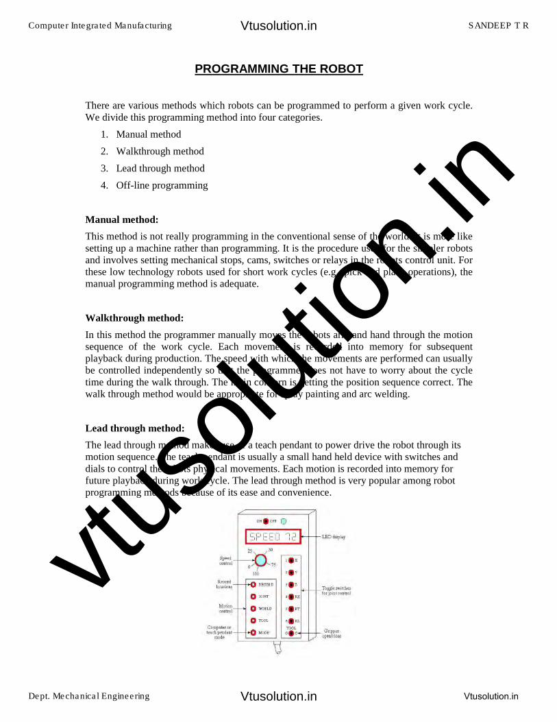
PROGRAMMING THE ROBOT
There are various methods which robots can be programmed to perform a given work cycle. We divide this programming method into four categories.
1. Manual method
2. Walkthrough method
3. Lead through method
4. Off-line programming
Manual method:
This method is not really programming in the conventional sense of the world. It is more like setting up a machine rather than programming. It is the procedure used for the simpler robots and involves setting mechanical stops, cams, switches or relays in the robots control unit. For these low technology robots used for short work cycles (e.g., pick and place operations), the manual programming method is adequate.
Walkthrough method:
In this method the programmer manually moves the robots arm and hand through the motion sequence of the work cycle. Each movement is recorded into memory for subsequent playback during production. The speed with which the movements are performed can usually be controlled independently so that the programmer does not have to worry about the cycle time during the walk through. The main concern is getting the position sequence correct. The walk through method would be appropriate for spray painting and arc welding.
Lead through method:
The lead through method makes use of a teach pendant to power drive the robot through its motion sequence. The teach pendant is usually a small hand held device with switches and dials to control the robots physical movements. Each motion is recorded into memory for future playback during work cycle. The lead through method is very popular among robot programming methods because of its ease and convenience.
Computer Integrated Manufacturing SANDEEP T R
Dept. Mechanical Engineering Vtusolution.in
Vtusolution.in
Vtusolution.in
vtuso
lution
.in
On-Line/Lead -Through programming
Advantage:
� Easy
� No special programming skills or training
Disadvantages:
� not practical for large or heavy robots
� High accuracy and straight-line movements are difficult to achieve, as are any other kind of geometrically defined trajectory, such as circular arcs, etc.
� difficult to edit out unwanted operator moves
� difficult to incorporate external sensor data
� Synchronization with other machines or equipment in the work cell is difficult
� A large amount of memory is required
Off- line programming:
This method involves the preparation of the robot program off-line, in a manner similar to NC part programming. Off-line robot programming is typically accomplished on a computer terminal. After the program has been prepared, it is entered in to the robot memory for use during the work cycle. The advantaged of off-line robot programming is that the production time of the robot is not lost to delay in teaching the robot a new task. Programming off-line can be done while the robot is still in production on the preceding job. This means higher utilization of the robot and the equipment with which it operates.
Another benefit associated with off-line programming is the prospect of integrating the robot into the factory CAD/CAM data base and information system.
Robot Programming Languages
Non computer controlled robots do not require programming language. They are programmed by the walkthrough or lead through methods while the simpler robots are programmed by manual methods. With the introduction of computer control for robots came the opportunity and the need to develop a computer oriented robot programming language.
The VALTM
Language
• The VAL language was developed for PUMA robot
• VAL stands for Victors Assembly Language
Computer Integrated Manufacturing SANDEEP T R
Dept. Mechanical Engineering Vtusolution.in
Vtusolution.in
Vtusolution.in
vtuso
lution
.in
• It is basically off-line language in which program defining the motion sequence is canbe developed off-line but various point location used in the work cycle are defined bylead through.
• VAL statements are divided into two categories a) Monitoring command b)Programming instructions.
• Monitor command are set of administrative instructions that direct the operation of therobot system. Some of the functions of Monitor commands are
Preparing the system for the user to write programs for PUMA
Defining points in space
Commanding the PUMA to execute a program
Listing program on the CRT
• Examples for monitor commands are: EDIT, EXECUTE, SPEED, HERE etc.
• Program instructions are a set of statements used to write robot programs. Onestatement usually corresponds to one movement of the robots arm or wrist.
• Example for program instructions are Move to point, move to a point in a straight linemotion, open gripper, close gripper. (MOVE, MOVES, APPRO, APPROS, DEPART,OPENI, CLOSEI, AND EXIT)
The MCL Language
• MCL stands for Machine Control Language developed by Douglas.
• The language is based on the APT and NC language. Designed control completemanufacturing cell.
• MCL is enhancement of APT which possesses additional options and features neededto do off-line programming of robotic work cell.
• Additional vocabulary words were developed to provide the supplementarycapabilities intended to be covered by the MCL. These capability include Vision,Inspection and Control of signals
• MCL also permits the user to define MACROS like statement that would beconvenient to use for specialized applications.
• MCL program is needed to compile to produce CLFILE.
• Some commands of MCL programming languages are DEVICE, SEND, RECEIV,WORKPT, ABORT, TASK, REGION, LOCATE etc.
Textual Statements
Language statements taken from commercially available robot languages
1 The basic motion statement is:
MOVE P1
Commands the robot to move from its current position to a position and orientation defined by the variable name P1.The point p1 must be defined.
Computer Integrated Manufacturing SANDEEP T R
Dept. Mechanical Engineering Vtusolution.in
Vtusolution.in
Vtusolution.in
vtuso
lution
.in
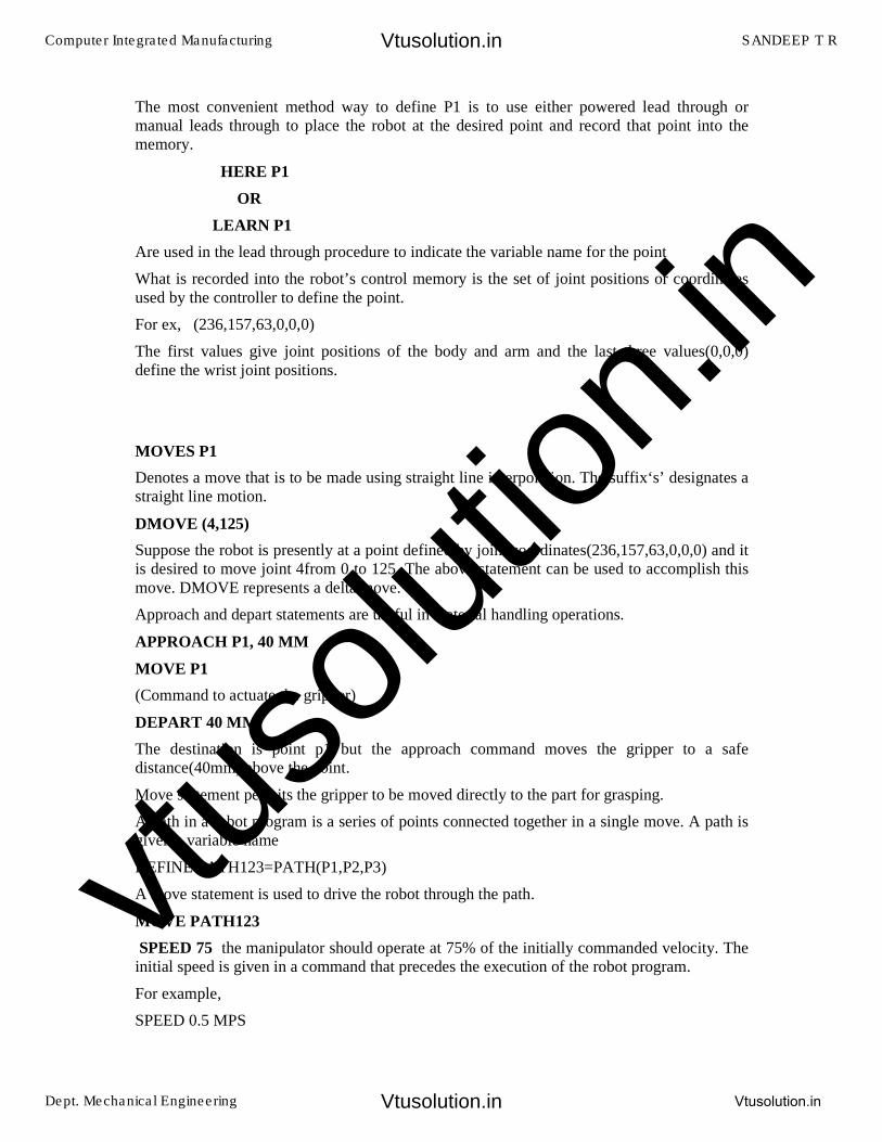
The most convenient method way to define P1 is to use either powered lead through or manual leads through to place the robot at the desired point and record that point into the memory.
HERE P1
OR
LEARN P1
Are used in the lead through procedure to indicate the variable name for the point
What is recorded into the robot’s control memory is the set of joint positions or coordinates used by the controller to define the point.
For ex, (236,157,63,0,0,0)
The first values give joint positions of the body and arm and the last three values(0,0,0) define the wrist joint positions.
MOVES P1
Denotes a move that is to be made using straight line interpolation. The suffix‘s’ designates a straight line motion.
DMOVE (4,125)
Suppose the robot is presently at a point defined by joint coordinates(236,157,63,0,0,0) and it is desired to move joint 4from 0 to 125. The above statement can be used to accomplish this move. DMOVE represents a delta move.
Approach and depart statements are useful in material handling operations.
APPROACH P1, 40 MM
MOVE P1
(Command to actuate the gripper)
DEPART 40 MM
The destination is point p1 but the approach command moves the gripper to a safe distance(40mm) above the point.
Move statement permits the gripper to be moved directly to the part for grasping.
A path in a robot program is a series of points connected together in a single move. A path is given a variable name
DEFINE PATH123=PATH(P1,P2,P3)
A move statement is used to drive the robot through the path.
MOVE PATH123
SPEED 75 the manipulator should operate at 75% of the initially commanded velocity. The initial speed is given in a command that precedes the execution of the robot program.
For example,
SPEED 0.5 MPS
Computer Integrated Manufacturing SANDEEP T R
Dept. Mechanical Engineering Vtusolution.in
Vtusolution.in
Vtusolution.in
vtuso
lution
.in
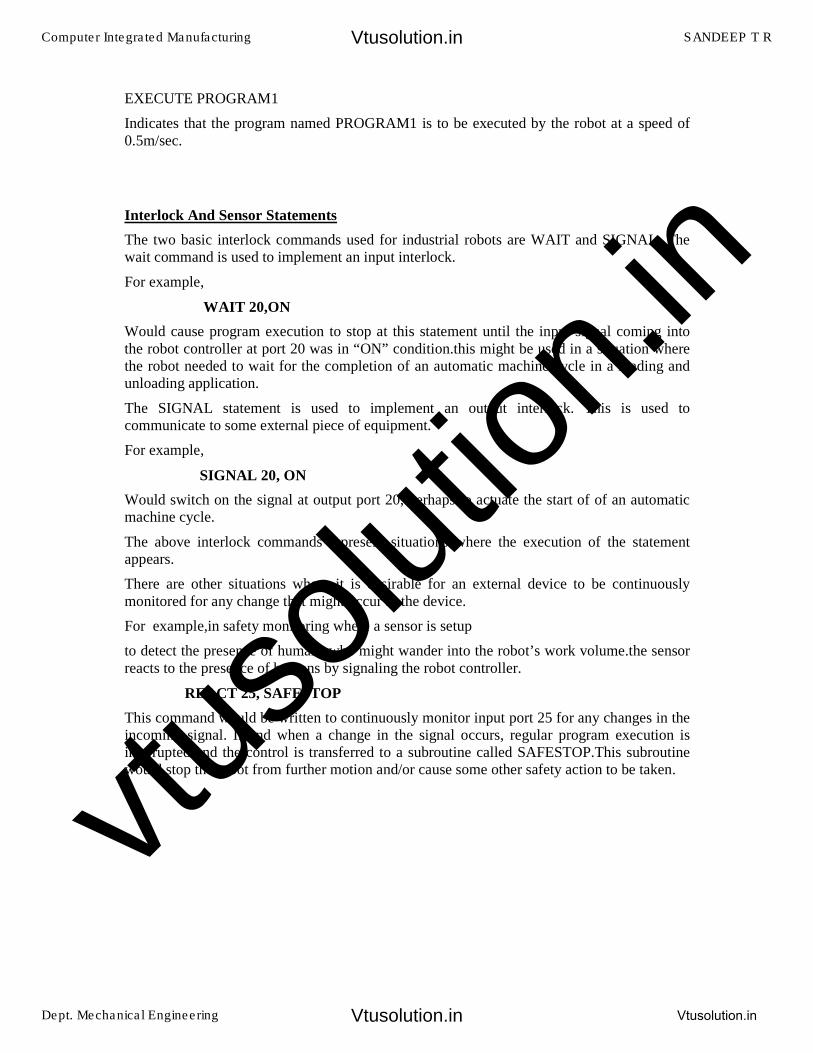
EXECUTE PROGRAM1
Indicates that the program named PROGRAM1 is to be executed by the robot at a speed of 0.5m/sec.
Interlock And Sensor Statements
The two basic interlock commands used for industrial robots are WAIT and SIGNAL. The wait command is used to implement an input interlock.
For example,
WAIT 20,ON
Would cause program execution to stop at this statement until the input signal coming into the robot controller at port 20 was in “ON” condition.this might be used in a situation where the robot needed to wait for the completion of an automatic machine cycle in a loading and unloading application.
The SIGNAL statement is used to implement an output interlock. This is used to communicate to some external piece of equipment.
For example,
SIGNAL 20, ON
Would switch on the signal at output port 20, perhaps to actuate the start of of an automatic machine cycle.
The above interlock commands represent situations where the execution of the statement appears.
There are other situations where it is desirable for an external device to be continuously monitored for any change that might occur in the device.
For example,in safety monitoring where a sensor is setup
to detect the presence of humans who might wander into the robot’s work volume.the sensor reacts to the presence of humans by signaling the robot controller.
REACT 25, SAFESTOP
This command would be written to continuously monitor input port 25 for any changes in the incoming signal. If and when a change in the signal occurs, regular program execution is interrupted and the control is transferred to a subroutine called SAFESTOP.This subroutine would stop the robot from further motion and/or cause some other safety action to be taken.
Computer Integrated Manufacturing SANDEEP T R
Dept. Mechanical Engineering Vtusolution.in
Vtusolution.in
Vtusolution.in
vtuso
lution
.in
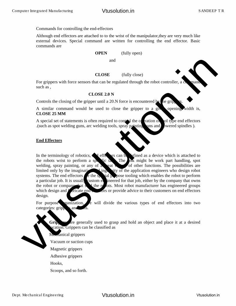
Commands for controlling the end-effectors
Although end effectors are attached to to the wrist of the manipulator,they are very much like external devices. Special command are written for controlling the end effector. Basic commands are
OPEN (fully open)
and
CLOSE (fully close)
For grippers with force sensors that can be regulated through the robot controller, a command such as ,
CLOSE 2.0 N
Controls the closing of the gripper until a 20.N force is encountered by the grippers.
A similar command would be used to close the gripper to a given opening width is, CLOSE 25 MM
A special set of statements is often required to control the operation of tool type end effectors .(such as spot welding guns, arc welding tools, spray painting guns and powered spindles ).
End Effectors
In the terminology of robotics, end effectors can be defined as a device which is attached to the robots wrist to perform a specific task. The task might be work part handling, spot welding, spray painting, or any of a great variety of other functions. The possibilities are limited only by the imagination and ingenuity of the application engineers who design robot systems. The end effectors are the special purpose tooling which enables the robot to perform a particular job. It is usually custom engineered for that job, either by the company that owns the robot or company that sold the robots. Most robot manufacturer has engineered groups which design and fabricate end effectors or provide advice to their customers on end effectors design.
For purpose organization, we will divide the various types of end effectors into two categories: grippers and tools.
1. Grippers: are generally used to grasp and hold an object and place it at a desiredlocation. Grippers can be classified as
Mechanical grippers
Vacuum or suction cups
Magnetic grippers
Adhesive grippers
Hooks,
Scoops, and so forth.
Computer Integrated Manufacturing SANDEEP T R
Dept. Mechanical Engineering Vtusolution.in
Vtusolution.in
Vtusolution.in
vtuso
lution
.in
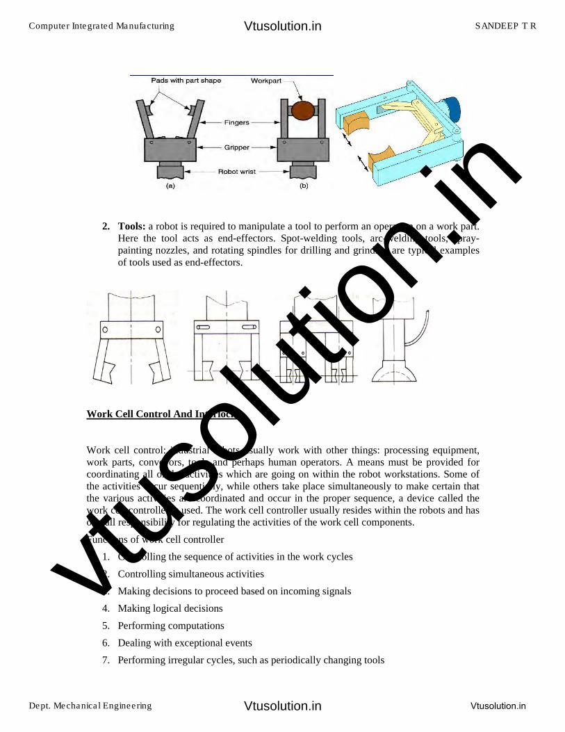
2. Tools: a robot is required to manipulate a tool to perform an operation on a work part.Here the tool acts as end-effectors. Spot-welding tools, arc-welding tools, spray-painting nozzles, and rotating spindles for drilling and grinding are typical examplesof tools used as end-effectors.
Work Cell Control And Interlocks
Work cell control: industrial robots usually work with other things: processing equipment, work parts, conveyors, tools and perhaps human operators. A means must be provided for coordinating all of the activities which are going on within the robot workstations. Some of the activities occur sequentially, while others take place simultaneously to make certain that the various activities are coordinated and occur in the proper sequence, a device called the work cell controller is used. The work cell controller usually resides within the robots and has overall responsibility for regulating the activities of the work cell components.
Functions of work cell controller
1. Controlling the sequence of activities in the work cycles
2. Controlling simultaneous activities
3. Making decisions to proceed based on incoming signals
4. Making logical decisions
5. Performing computations
6. Dealing with exceptional events
7. Performing irregular cycles, such as periodically changing tools
Computer Integrated Manufacturing SANDEEP T R
Dept. Mechanical Engineering Vtusolution.in
Vtusolution.in
Vtusolution.in
vtuso
lution
.in
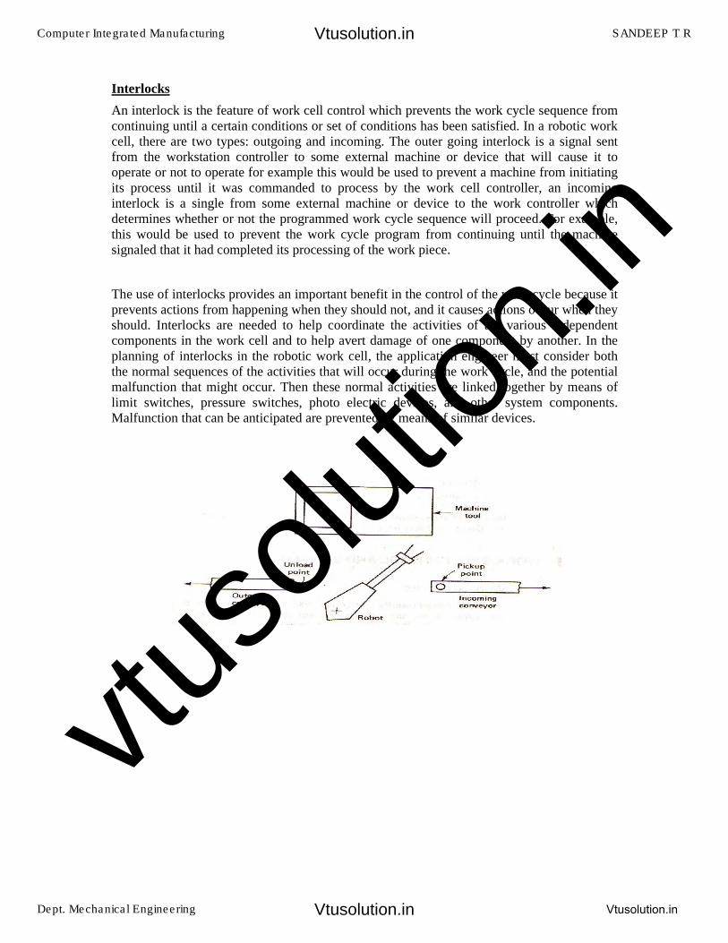
Interlocks
An interlock is the feature of work cell control which prevents the work cycle sequence from continuing until a certain conditions or set of conditions has been satisfied. In a robotic work cell, there are two types: outgoing and incoming. The outer going interlock is a signal sent from the workstation controller to some external machine or device that will cause it to operate or not to operate for example this would be used to prevent a machine from initiating its process until it was commanded to process by the work cell controller, an incoming interlock is a single from some external machine or device to the work controller which determines whether or not the programmed work cycle sequence will proceed. For example, this would be used to prevent the work cycle program from continuing until the machine signaled that it had completed its processing of the work piece.
The use of interlocks provides an important benefit in the control of the work cycle because it prevents actions from happening when they should not, and it causes actions occur when they should. Interlocks are needed to help coordinate the activities of the various independent components in the work cell and to help avert damage of one component by another. In the planning of interlocks in the robotic work cell, the application engineer must consider both the normal sequences of the activities that will occur during the work cycle, and the potential malfunction that might occur. Then these normal activities are linked together by means of limit switches, pressure switches, photo electric devices, and other system components. Malfunction that can be anticipated are prevented by means of similar devices.
Computer Integrated Manufacturing SANDEEP T R
Dept. Mechanical Engineering Vtusolution.in
Vtusolution.in
Vtusolution.in
vtuso
lution
.in
ROBOTIC SENSORS
For certain robot application, the type of workstation control using interlocks is not adequate the robot must take on more human like senses and capabilities in order to perform the task in a satisfactory way these senses and capability includes vision and hand eye coordination, touch, hearing accordingly we will dived the types of sensors used in robotics into the following three categories.
1. Vision sensors
2. Tactile and proximity sensors
3. Voice sensors
Vision sensors
This is one of the areas that is receiving a lot of attention in robotics research computerized visions systems will be an important technology in future automated factories. Robot vision is made possible by means of video camera a sufficient light source and a computer programmed to process image data. The camera is mounted either on the robot or in a fixed position above the robot so that its field of vision includes the robots work volume. The computer software enables the vision system to sense the presence of an object and its position and orientation. Vision capability would enable the robot to carry out the following kinds of operations.
Retrieve parts which are randomly oriented on a conveyor
Recognize particular parts which are intermixed with other objects
Perform assembly operations which require alignment
Tactile and proximity sensor
Tactile sensors provide the robot with the capability to respond to contact forces between itself and other objects within its work volume. Tactile sensors can be divided into two types:
1. Touch sensors
2. Stress sensors
Touch sensors are used simply to indicate whether contact has been made with an object. A simple micro switch can serve the purpose of a touch sensor. Stress sensors are used to measure the magnitude of the contact force. Strain gauge devices are typically employed in force measuring sensors.
Potential use of robots with tactile sensing capabilities would be in assembly and inspection operations. In assembly, the robot could perform delicate part alignment and joining operations. In inspection, touch sensing would be used in gauging operations and dimensional measuring activities. Proximity sensors are used to sense when one object is close to another
Computer Integrated Manufacturing SANDEEP T R
Dept. Mechanical Engineering Vtusolution.in
Vtusolution.in
Vtusolution.in
vtuso
lution
.in
object. On a robot, the proximity sensors would be located n or near the end effectors. This sensing capability can be engineered by means of optical proximity devices, eddy-current proximity detectors, magnetic field sensors, or other devices.
In robotics, proximity sensors might be used to indicate the presence or absence of a work part or other object. They could also be helpful in preventing injury to the robots human coworkers in the factory.
Voice sensors
Another area of robotics research is voice sensing or voice programming. Voice programming can be defined as the oral communication of commands to the robot or other machine. The robot controller is equipped with a speech recognition system which analyzes the voice input and compares it with a set of stored word patterns when a match is found between the input and the stored vocabulary word the robot performs some actions which corresponds to the word. Voice sensors could be useful in robot programming to speed up the programming procedure just as it does in NC programming. It would also be beneficial in especially in hazardous working environments for performing unique operations such as maintenance and repair work. The robot could be placed in hazardous environment and remotely commanded to perform the repair chores by means of step by step instructions.
Sensors – summary
• Sensors provide a way of simulating “aliveness”
• Sensors give robots environmental awareness
• Sensors provide of means of human protection
• Sensors help robot preserve itself
• Sensors enable goal seeking
• Sensors enable closed-loop interaction
• Sensors make robots interesting
• Sensors can make programming “challenging”
Computer Integrated Manufacturing SANDEEP T R
Dept. Mechanical Engineering Vtusolution.in
Vtusolution.in
Vtusolution.in
vtuso
lution
.in

ROBOT APPLICATIONS
Need to replace human labor by robots:
• Work environment hazardous for human beings
• Repetitive tasks
• Boring and unpleasant tasks
• Multi shift operations
• Infrequent changeovers
• Performing at a steady pace
• Operating for long hours without rest
• Responding in automated operations
• Minimizing variation
Industrial Robot Applications can be divided into:
Material-handling applications:
• Involve the movement of material or parts from one location to another.
• It includes part placement, palletizing and/or depalletizing, machineloading and unloading.
Processing Operations:
• Requires the robot to manipulate a special process tool as the endeffectors.
• The application include spot welding, arc welding, riveting, spray painting,machining, metal cutting, deburring, polishing.
Assembly Applications:
• Involve part-handling manipulations of a special tools and other automatictasks and operations.
Inspection Operations:
• Require the robot to position a work part to an inspection device.
• Involve the robot to manipulate a device or sensor to perform theinspection.
Material Handling Applications
This category includes the following:
• Part Placement
• Palletizing and/or depalletizing
Computer Integrated Manufacturing SANDEEP T R
Dept. Mechanical Engineering Vtusolution.in
Vtusolution.in
Vtusolution.in
vtuso
lution
.in
• Machine loading and/or unloading
• Stacking and insertion operations
Part Placement:
• The basic operation in this category is the relatively simple pick-and-placeoperation.
• This application needs a low-technology robot of the cylindricalcoordinate type.
• Only two, three, or four joints are required for most of the applications.
• Pneumatically powered robots are often utilized.
Palletizing and/or Depalletizing
• The applications require robot to stack parts one on top of the other, that isto palletize them, or to unstack parts by removing from the top one by one,that is depalletize them.
• Example: process of taking parts from the assembly line and stacking themon a pallet or vice versa.
Machine loading and/or unloading:
• Robot transfers parts into and/or from a production machine.
• There are three possible cases:
� Machine loading in which the robot loads parts into a productionmachine, but the parts are unloaded by some other means.
Example: a press working operation, where the robot feeds sheet blanks into the press, but the finished parts drop out of the press by gravity.
� Machine loading in which the raw materials are fed into the machine without robot assistance. The robot unloads the part from the machine assisted by vision or no vision.
Example: bin picking, die casting, and plastic moulding.
� Machine loading and unloading that involves both loading and unloading of the work parts by the robot. The robot loads a raw work part into the process ad unloads a finished part.
Example: Machine operation difficulties
Computer Integrated Manufacturing SANDEEP T R
Dept. Mechanical Engineering Vtusolution.in
Vtusolution.in
Vtusolution.in
vtuso
lution
.in
• Difference in cycle time between the robot and the production machine.The cycle time of the machine may be relatively long compared to therobot’s cycle time.
Stacking and insertion operation:
• In the stacking process the robot places flat parts on top of each other,where the vertical location of the drop-off position is continuouslychanging with cycle time.
• In the insertion process robot inserts parts into the compartments of adivided carton.
The robot must have following features to facilitate material handling:
• The manipulator must be able to lift the parts safely.
• The robot must have the reach needed.
• The robot must have cylindrical coordinate type.
• The robot’s controller must have a large enough memory to store all theprogrammed points so that the robot can move from one location toanother.
• The robot must have the speed necessary for meeting the transfer cycle ofthe operation.
Processing operations:
• Robot performs a processing procedure on the part.
• The robot is equipped with some type of process tooling as its end effector.
• Manipulates the tooling relative to the working part during the cycle.
• Industrial robot applications in the processing operations include:
� Spot welding
� Continuous arc welding
� Spray painting
� Metal cutting and deburring operations
� Various machining operations like drilling, grinding, laser and water jet cutting, and riveting.
� Rotating and spindle operations
� Adhesives and sealant dispensing
Computer Integrated Manufacturing SANDEEP T R
Dept. Mechanical Engineering Vtusolution.in
Vtusolution.in
Vtusolution.in
vtuso
lution
.in
Assembly operations:
• The applications involve both material-handling and the manipulation of a tool.
• They typically include components to build the product and to perform materialhandling operations.
• Are traditionally labor-intensive activities in industry and are highly repetitive andboring. Hence are logical candidates for robotic applications.
• These are classified as:
� Batch assembly: As many as one million products might be assembled.
� The assembly operation has long production runs.
� Low-volume: In this a sample run of ten thousand or less products might be made.
� The assembly robot cell should be a modular cell.
� One of the well suited areas for robotics assembly is the insertion of odd electronic components.
Inspection operation:
• Some inspection operation requires parts to be manipulated, and other applicationsrequire that an inspection tool be manipulated.
• Inspection work requires high precision and patience, and human judgment isoften needed to determine whether a product is within quality specifications ornot.
• Inspection tasks that are performed by industrial robots can usually be divided intothe following three techniques:
� By using a feeler gauge or a linear displacement transducer known as a linear variable differential transformer (LVDT), the part being measured will come in physical contact with the instrument or by means of air pressure, which will cause it to ride above the surface being measured.
� By utilizing robotic vision, matrix video cameras are used to obtain an image of the area of interest, which is digitized and compared to a similar image with specified tolerance.
� By involving the use of optics and light, usually a laser or infrared source is used to illustrate the area of interest.
• The robot may be in active or passive role.
� In active role robot is responsible for determining whether the part is good or bad.
� In the passive role the robot feeds a gauging station with the part. While the gauging station is determining whether the part meets the specification, the robot waits for the process to finish.
Computer Integrated Manufacturing SANDEEP T R
Dept. Mechanical Engineering Vtusolution.in
Vtusolution.in
Vtusolution.in
vtuso
lution
.in
Advantages of Robots
• Robotics and automation can, in many situation, increase productivity, safety,efficiency, quality, and consistency of Products
• Robots can work in hazardous environments
• Robots need no environmental comfort
• Robots work continuously without any humanity needs and illnesses
• Robots have repeatable precision at all times
• Robots can be much more accurate than humans, they may have milli or micro inchaccuracy.
• Robots and their sensors can have capabilities beyond that of humans.
• Robots can process multiple stimuli or tasks simultaneously, humans can only one.
• Robots replace human workers who can create economic problems.
Disadvantages of Robots
• Robots lack capability to respond in emergencies, this can cause:
� Inappropriate and wrong responses
� A lack of decision-making power
� A loss of power
� Damage to the robot and other devices
� Human injuries
• Robots may have limited capabilities in
� Degrees of Freedom
� Dexterity
� Sensors
� Vision systems
� Real-time Response
• Robots are costly, due to
� Initial cost of equipment
� Installation Costs
� Need for peripherals
� Need for training
� Need for Programming
Computer Integrated Manufacturing SANDEEP T R
Dept. Mechanical Engineering Vtusolution.in
Vtusolution.in
Vtusolution.in
vtuso
lution
.in
Summary of Robot Applications
General characteristics of industrial work situations that promote the use of industrial robots
1. Hazardous work environment for humans
2. Repetitive work cycle
3. Difficult handling task for humans
4. Multi shift operations
5. Infrequent changeovers
6. Part position and orientation are established in the work cell
Computer Integrated Manufacturing SANDEEP T R
Dept. Mechanical Engineering Vtusolution.in
Vtusolution.in
Vtusolution.in
vtuso
lution
.in