Lesson no. 17QUALITIES OF GOOD DATA-GATHERING

PROCEDURES

When many people think of research, they imagine numbers and statistics. However, the numbers that are gathered are based on various data gathering techniques as outlined in Section 1 of this chapter. The quality of these procedures is determined by the caliber of the data-gathering strategy. To sharpen our ability to discern between weak and strong research, we must give attention to this aspect of research when evaluating the worth of a study. The purpose of this section is to provide an overview of these qualities and give examples of how they have been applied in research. My goal is for you to be able to use these qualities as criteria to evaluate the quality of the research that you read in a discerning manner. The two most important qualities of any data-collection technique that have traditionally been considered essential are reliability and validity. The strong consensus in the measurement community is that the level of confidence we can put into the findings of any given research is directly proportional to the degree to which data-gathering procedures are reliable and valid. I begin by discussing reliability, followed by validity. Some research methodology books place their section on validity before reliability. However, because validity relies heavily on reliability, I discuss the latter first.

Reliability

Reliability has to do with the consistency of the data results. If we measure or observe something, we want the method used to give the same results no matter who or what takes the measurement or observations. Researchers who use two or more observers would want those observers to see the same things and give the same or similar judgments on what they observe or rate. Likewise, researchers utilizing instruments would expect them to give consistent results regardless of time of administration or the particular set of test items making up those instruments. The most common indicator used for reporting the reliability of an observational or instrumental procedure is the correlation coefficient. A coefficient is simply a number that represents the amount of attribute. A correlation coefficient is a number that quantifies the degree to which two variables relate to one another. Correlation coefficients used to indicate reliability are referred to as reliability coefficients. I do not go into the mathematics of this particular statistic, but I want to give enough information to help in understanding the following discussion. Reliability coefficients range between 0.00 and +1.00. A coefficient of 0.00 means there is no reliability in the observation or measurement. That is, if we were to make multiple observations/measurements of a particular variable, a coefficient of 0.00 would mean that the observations/measurements were inconsistent. Conversely, a coefficient of 1.00 indicates that there is perfect reliability or consistency. This means that the observation/measurement procedure gives the same results regardless of who or what makes the observation/measurement. Seldom, if ever, do reliability coefficients occur at the extreme ends of the continuum (i.e., 0.00 or 1.00). So, you might ask, “What is an adequate reliability coefficient?” The rule of thumb is,

the higher the better (Wow, that was a no-brainer!!!), but better depends on the nature of the measurement procedure being used. Researchers using observation techniques involving judges are happy with reliability coefficients anywhere from 0.80 on up. Yet achievement and aptitude tests should have reliabilities in the 0.90s. Other instruments such as interest inventories and attitude scales tend to be lower than achievement or aptitude tests. Generally speaking, reliabilities falling below 60 are considered low no matter what type of procedure is being used (Nitko, 2001). There are a number of different types of reliability coefficients used in research. The reason is that each one reveals a different kind of consistency. Different measurement procedures require different kinds of consistency. Table 6.2 lists the different types of reliability coefficients, what kind of consistency is needed, and the corresponding measurement procedure. The first one listed, interrater or interobserver reliability, is required any time different observers are used to observe or rate participants’ behavior. Researchers typically determine the reliability of the observers/raters by either computing a correlation coefficient or calculating a percentage of agreement. The study discussed in chapter 5 by Bejarano et al. (1997) used two independent raters for their observational procedures. They reported interrater reliabilities for the three variables as 0.98, 0.86, and 0.96. These figures reveal high agreement among the raters, which I am sure pleased the researchers.

Also related to the use of observers/raters is intrarater reliability. The type of consistency this addresses relates to observers/raters giving the same results if they were given the opportunity to observe/rate participants on more than one occasion. We would expect high agreement within the same person doing the observing/rating over time if the attribute being observed is stable and the observer/rater understood the task. However, if the observer/rater is not clear about what s/he is supposed to observe/rate, there will be different results, and

correlations or percentages of agreement will be low. Although this is an important issue, I have not seen many recent studies report this type of reliability. One example I did find was Goh’s (2002) study, mentioned in chapter 5, which used both inter- and intrarater reliability. Recall that her study looked at listening comprehension techniques and how they interacted with one another. She had two participants read passages with pauses. During each pause, they were to reflect on how they attempted to understand the segment they heard. These retrospections were taped and transcribed. The transcriptions were analyzed by Goh, identifying, interpreting, and coding the data. Commendably, she checked the reliability of her observations by enlisting a colleague to follow the same procedures on a portion of the data and computing an interrater reliability coefficient (r = 0.76). In addition, she computed an intrarater reliability coefficient (r = 0.88) to make sure there was consistency even within her own observations. As expected, she agreed with herself (intrarater) more than she agreed with her colleague (interrater). The remainder of the other types of reliabilities in Table 6.2 are used with paper-and-pencil or computer-administered instruments, whether questionnaires or tests. Test–retest reliability is used to measure the stability of the same instrument over time. The instrument is given at least twice, and a correlation coefficient is computed on the scores. However, this procedure can only work if the trait (i.e., construct) being measured can be assumed to remain stable over the time between the two measurements. For example, if the researcher is assessing participants’ L2 pronunciation abilities, administering the instrument 2 weeks later should produce similar results if it is reliable. However, if there is a month or two between testing sessions, any training on pronunciation may create differences between the two sets of scores that would depress the reliability coefficient. However, if the time between the two administrations is too little, memory of the test from the first session could help the participants give the same responses, which would inflate the reliability coefficient. A study that reported a test–retest reliability (Camiciottoli, 2001) was mentioned in Section 1 of this chapter. Camiciottoli used a 22-item questionnaire to collect data on both independent and dependent variables. To measure test–retest reliability, she gave 20 participants from the larger group the same questionnaire 6 weeks later. She then correlated the results from the first administration with that of the second and found a reliability coefficient of 0.89. This is considered fairly high reliability. Another type of reliability estimate typically used when a test has several different forms is the alternate-form procedure. Most standardized tests have multiple forms to test the same attribute. The forms are different in that the items are not the same, but they are similar in form and content. To ensure that each form is testing the same trait, pairs of different forms are given to the same individuals with several days or more between administrations. The results are then correlated. If the different forms are testing the same attribute, the correlations should be fairly high. Not only does this procedure test stability of results over time, it also tests whether the items in the different forms represent the same general attribute being tested. For example, if researchers were to use the Cambridge Certificate in Advanced English (CAE) test battery5 in a research study, they would need assurance from the test publisher that, no matter what form was used, the results would reveal a similar measure of English language proficiency. Again researchers

should report the alternate-form reliability coefficient provided by the test publisher in his or her research report.

The assumption cannot be made by researchers that those who read the study will know that a particular standardized test is reliable even if it is well known. No matter what test is used, the reliability should be reported in any study where applicable. A practice that you will no doubt see in your perusal of research is that of borrowing parts of commercially produced standardized tests to construct other tests. It seems that researchers doing this are under the assumption that, because items come from an instrument that has good reliability estimates, any test consisting of a subset of borrowed items will inherit the same reliability. This cannot be taken for granted. Test items often behave differently when put into other configurations. For this reason, subtests consisting of test items coming from such larger, proven instruments should be reevaluated for reliability before using them in a study. Rodriguez and Sadoski (2000), mentioned earlier, in addition to developing their own 15-item Spanish test, took 15 items from the Green and Purple Levels of the Stanford Diagnostic Reading Test for use in their English test. It would have been helpful if they had reported the reliabilities for these smaller tests. If reliability information were not available from the test publishers, they could have calculated their own reliabilities. Without knowing the reliability of a test, there is no way to know how consistent the results are. The last three methods of estimating the reliability of a test are concerned with the internal consistency of the items within the instrument. In other words, do all the items in an instrument measure the same general attribute? This is important because the responses for each item are normally added up to make a total score. If the items are measuring different traits, then a total score would not make much sense. To illustrate, if a researcher tries to measure participant attitudes toward a second language, do all of the items in the survey 6 contribute to reflecting their attitude? If some items are measuring grammar ability, then combining their results with those of the attitude items would confound the measure of attitude.

The first of these three methods presented is known as split-half (odd/even). It is the easiest of the three methods to compute. As the name suggests, the items in the test are divided in half. Responses on each half are added up to make a subtotal for each half. This can be done by simply splitting the test in half, which is appropriate if the second half of the items is not different in difficulty level or the test is not too long. The reason that length is a factor is respondents might become tired in the latter half of the test, which would make their responses different from the first half of the test. To get around these problems, the test can be divided by comparing the odd items with the even items. The responses on the items for each respondent are divided into two subtotals—odd and even. That is, the odd items (e.g., Items 1, 3, 5, etc.) are summed and compared with the sum of the even items (e.g., Items 2, 4, 6, etc.). The odd/even method is preferred because it is not influenced by the qualitative change in items that often occur in different sections of the instrument, such as difficulty of item or fatigue.

Factors that affect reliability are numerous. One of the major factors is the degree to which the instrument or procedure is affected by subjectivity of the people doing the rating or

scoring. The more a procedure is vulnerable to perceptual bias, lack of awareness, fatigue, or anything else that influences the ability to observe or rate what is happening, the lower the reliability. Other factors that affect reliability are especially related to discrete-point item7 tests for collecting data. One of these is test length, which can affect reliability in two different ways. The first involves not having enough items. Instruments with fewer items will automatically produce smaller reliability coefficients. This is not necessarily due to the items being inconsistent, but rather is a simple mathematical limitation inherent to correlation coefficients. However, there is a correction formula known as the Spearman-Brown prophecy formula (Nitko, 2001), which is available for use. This is used to project what the reliability estimate would be if the test had more items. When researchers use the split-half reliability coefficient (cf. Table 6.2), they usually report the Spearman-Brown coefficient because the test has been cut into halves, creating two short tests. Garcia and Asencion (2001) followed this procedure in their study, which looked at the effects of group interaction on language development. They used two tasks for collecting data: a text reconstruction test and a test of listening comprehension. The first test was scored using two raters who were looking at the correct use of three grammar rules. They reported interrater reliability with a correlation coefficient of 0.98: very high. For the listening test, which only consisted of 10 items, they used the split-half method along with the Spearman-Brown adjustment for a short test (r = 0.73). This appears to be moderate reliability, but remember that it was a short test. So, in fact, the correlation is not bad.

The second way that the length of an instrument can affect reliability is when it is too long. Responses to items that are in the latter part of the instrument can be affected by fatigue. Respondents who are tired will not produce consistent responses, which will lower reliability coefficients. When developing an English language test battery for placing students at the university where I teach, my development team and I noticed that the reliability of the reading component was lower than expected. This component was the last test in the battery. On further investigation, we found that a number of items in the last part of the test were not being answered. Our conclusion was that the test takers were running out of time or energy and were not able to finish the last items. We corrected the problem, and the reliability of this component increased to the level we felt appropriate. This is also a problem with long surveys.

The final factor I mention is the item quality used in an instrument. Ambiguous test items will produce inconsistent results and lower reliability. Participants will guess at poorly written items, and this will not give an accurate measure of the attribute under observation. Items that have more than one correct answer or are written to trick the participant will have similar negative effects. Scarcella and Zimmerman (1998), for example, dropped 10 items from their Test of Academic Lexicon because these items lowered the Cronbach alpha coefficient. For some reason, these items were not consistently measuring the same attribute as the rest of the instrument. This left them with 40 real-word items, which they considered adequate. There are other factors that influence reliability coefficients, but they relate to correlation coefficients in general. I raise these issues in the next chapter when discussing correlation coefficients in greater

detail. However, to emphasize how important knowing what the reliability of an instrument is, I introduce you to the Standard Error of Measurement (SEM; Hughes, 2003; Nitko, 2001). Don’t let this term make you nervous; it is not as bad as it looks. I will attempt to explain this in a nonmathematical way. The reliability coefficient is also used to estimate how much error there is in the measurement procedure—error is any variation in the instrument results due to factors other than what is being measured. By performing some simple math procedures on the reliability coefficient, an estimate of the amount of error is calculated, referred to as the SEM. If there is perfect reliability (i.e., r = 1.00), there is no error in the measurement; that is, there is perfect consistency. This means that any difference in scores on the instrument can be interpreted as true differences between participants. However, if there is no reliability (i.e., r = 0.00), then no difference between participant scores can be interpreted as true difference on the trait being measured. To illustrate, if I used a procedure for measuring language proficiency that had no reliability, although I might get a set of scores differing across individuals, I could not conclude that one person who scored higher than another had a higher proficiency. All differences would be contributed to error from a variety of unknown sources.

Validity

As with reliability, the quality of validity is more complex than initially appears. On the surface, people use it to refer to the ability of an instrument or observational procedure to accurately capture data needed to answer a research question. On the other hand, many research methodology textbooks distinguish among a number of types of validity, such as content validity, predictive validity, face validity, construct validity, and so on (e.g., Brown, 1988; Gall et al., 1996; Hatch & Lazaraton, 1991). These different types have led to some confusion. For instance, I have heard some people accuse certain data-gathering procedures of being invalid, whereas others claim that the same procedures are valid. However, when their arguments are examined more closely, one realizes that the two sides of the debate are using different definitions of validity. Since the early 1990s, the prior notions of validity have been subsumed under the heading of construct validity (Bachman, 1990; Messick, 1989). These types of validity are now represented as different facets of validity under this global title. They are summarized in Table 6.3.

In the upper half of Table 6.3 in the left column, validity is shown to be comprised of two main facets: trait accuracy and utility. Trait accuracy, which corresponds with the former construct validity, addresses the question as to how accurately the procedure measures the trait (i.e., construct) under investigation. However, accuracy depends on the definition of the construct being measured or observed. Language proficiency, for example, is a trait that is often measured in research. Nevertheless, how this trait is measured should be determined by how it is defined. If language proficiency is defined as the summation of grammar and vocabulary knowledge, plus reading and listening comprehension, then an approach needs to be used that measures all of these components to accurately measure the trait as defined.

However, if other researchers define language proficiency as oral and writing proficiency, they would have to use procedures to directly assess speaking and writing ability. In other words, the degree to which a procedure is valid for trait accuracy is determined by the degree to which the procedure corresponds to the definition of the trait. When reading a research article, the traits need to be clearly defined to know whether the measurements used are valid in regards to the accuracy facet of validity. These definitions should appear in either the introduction or methodology section of the article. To illustrate, in their search for factors contributing to second language learning, Gardner et al. (1997) defined language anxiety as “communication apprehension, test anxiety, and fear of negative evaluation” (pp. 344–345) based on the Foreign Language Classroom Anxiety Scale developed by Horwitz, Horwitz, and Cope (1986; cited in Gardner et al., 1997). This practice of defining traits by using already existing instruments is common among researchers. In effect, the instrument provides the operational definition of the trait. Regarding the second main facet of validity, utility is concerned with whether measurement/observational procedures are used for the right purpose. If a procedure is not used for what it was originally intended for, there might be a question as to whether it is a valid procedure for obtaining the data needed in a particular study. If it is used for something other than what it was originally designed to do, the researcher must provide additional evidence that the procedure is valid for the purpose of his or her study.

For example, if you wanted to use the results from the TOEFL to measure the effects of a treatment over a 2-week training period, this would be invalid. To reiterate, the reason is that the TOEFL was designed to measure language proficiency, which develops over long periods of time. It was not designed to measure the specific outcomes that the treatment was targeting. Note in Table 6.3 that there are three other facets that further qualify the main facets of trait accuracy and utility: criterion related, content coverage, and face appearance. These used to be referred to as separate validities: criterion-related validity, content validity, and face validity (e.g., Brown, 1988). However, within the current global concept of construct validity, they help define the complex nature of validity. Criterion related simply means that the procedure is validated by being compared to some external criterion. It is divided into two general types of trait accuracy: capacity to succeed and current characteristics. Capacity to succeed relates to a person having the necessary wherewithal or aptitude to succeed in some other endeavor. Typically, this involves carefully defining the aptitude being measured and then constructing or finding an instrument or observational procedure that would accurately obtain the needed data. The utility of identifying people’s capacity to succeed is usually for prediction purposes. For instance, if a researcher wants to predict people’s ability to master a foreign language, s/he would administer a procedure that would assess whether the examinees had the necessary aptitude to succeed.

Predictive utility is determined by correlating the measurements from the procedures with measurements on the criterion being predicted. I do not go into further detail about how this is done; suffice it to say that you can find more about this from any book on assessment (e.g., Nitko, 2001). A number of measures have been used over the years to predict the success of students in acquiring a second language. One of the most well-known standardized instruments that has been around for many years is the Modern Language Aptitude Test developed by Carroll and Sapon (1959). They developed this test for the purpose of predicting whether people have an aptitude for learning languages. Steinman and Smith (2001) presented evidence in their review of this test that it is not only valid for making predictions, but it has become used as an external criterion for validating other tests.

Lesson no. 18Understanding research results

Some people think that numerical data are more scientific—and therefore more important—than verbal data because of the statistical analyses that can be performed on numerical data. However, this is a false conclusion. We must not forget that numbers are only as good as the constructs they represent. In other words, when we use statistics, we have basically transferred verbally defined constructs into numbers so we can analyze the data more easily. We must not forget that these statistical results must again be transferred back into terminology that represents these verbal constructs to make any sense.

Common Procedure

In almost all studies, all of the data that have been gathered are not presented in the research report. Whether verbal or numerical, the data presented have gone through some form of selection and reduction. The reason is that both verbal and numerical data typically are voluminous in their rawest forms. What you see reported in a research journal are results of the raw data having been boiled down into manageable units for display to the public. Verbal data commonly appear as selections of excerpts, narrative vignettes, and quotations from interviews, and so on, whereas numerical data are often condensed into tables of frequencies, averages, and so on. There are some interesting differences, however, which I describe in the following two sections.

SECTION 1: PRESENTATION AND ANALYSISOF VERBAL DATA

Presentation of verbal data and their analyses appear very much intertwined together in Results sections of research reports. That is, separating the data from the analysis is difficult. Numerical data, in contrast, are presented in some type of summarized form (i.e., descriptive statistics) and followed with the analysis in the form of inferential statistics.

Consequently, the analysis of verbal data is not quite as straightforward as the analysis of numerical data. The reason is that analysis of verbal data is initiated at the beginning of the data-collection process and continues throughout the study. This process involves the researcher interacting with the data in a symbiotic fashion. Literally, the researcher becomes the “main ‘measurement device’ ” (Miles & Huberman, 1994, p. 7). Creswell (1998, pp. 142–143) likened data analysis to a “contour” in the form of a “data analysis spiral,” where the researcher engages the data, reflects, makes notes, reengages the data, organizes, codes, reduces the data, looks for relationships and themes, makes checks on the credibility of the emerging system, and eventually draws conclusions.

However, when we read published qualitative research, we seldom are given a clear description of how this data analysis spiral transpired. In Miles and Huberman’s (1994) words, “We rarely see data displays—only the conclusions. In most cases we don’t see a procedural account of the analysis, explaining just how the researcher got from 500 pages of field notes to the main conclusions drawn” (p. 262). If the researcher is working alone during the data analysis spiral, serious questions arise concerning the credibility of any conclusions made. First, there is

the problem mentioned in chapter 6 regarding possible bias when gathering data through observation and other noninstrumental procedures. However, because analysis begins during the data-collection stage in qualitative research, analytical biases become a possible threat to the validity of conclusions. Miles and Huberman (1994) identified three archetypical ones: holistic fallacy, elite bias, and going native. The first has to do with seeing patterns and themes that are not really there. The second is concerned with giving too much weight to informants who are more articulate and better informed, making the data unrepresentative. The third, going native, occurs when the researcher gets so close to the respondents that s/he is “co-opted into [their] perceptions and explanations” (p. 264).

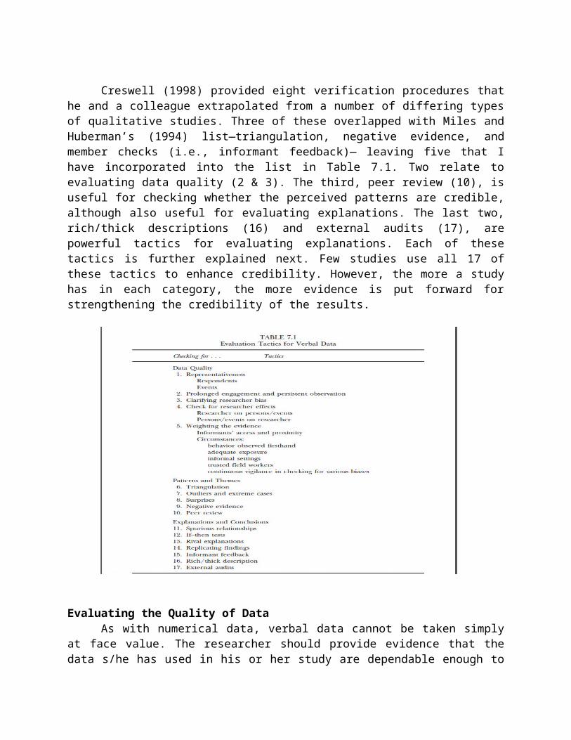
Creswell (1998) provided eight verification procedures that he and a colleague extrapolated from a number of differing types of qualitative studies. Three of these overlapped with Miles and Huberman’s (1994) list—triangulation, negative evidence, and member checks (i.e., informant feedback)— leaving five that I have incorporated into the list in Table 7.1. Two relate to evaluating data quality (2 & 3). The third, peer review (10), is useful for checking whether the perceived patterns are credible, although also useful for evaluating explanations. The last two, rich/thick descriptions (16) and external audits (17), are powerful tactics for evaluating explanations. Each of these tactics is further explained next. Few studies use all 17 of these tactics to enhance credibility. However, the more a study has in each category, the more evidence is put forward for strengthening the credibility of the results.

Evaluating the Quality of DataAs with numerical data, verbal data cannot be taken simply at face value. The researcher

should provide evidence that the data s/he has used in his or her study are dependable enough to

analyze. The researcher has at least five strategies to choose from to support the quality of the data. They are as follows:

1. Representativeness: This is not referring specifically to whether the sample is representative of the population. This is more to do with whether the veracity of the information is being influenced by the choice of respondents or events (i.e., internal validity or credibility). Related to the elite bias mentioned earlier, information coming from one particular segment of a larger group of people can be misleading. The most accessible and willing informants are not usually the best group to provide the most appropriate data.

In addition, the researcher needs to give evidence that the events on which generalizations are based are the most appropriate. A researcher might not be present at all times for data collection. If not, the consumer must ask about the proportion of time the researcher was present. If only a fraction of the events were observed, were they typical of most events? The ultimate question for the consumer is whether the researcher has provided evidence that data have come from observing an adequate number of events to ensure that subsequent inferences and conclusions were not based on the luck of the draw.

2. Prolonged engagement and persistent observation: The researcher needs enough time to interact with the respondents and/or the event to gather accurate data. This allows the researcher time to gain personal access to the information being targeted. However, if too much time is spent on the research site, there is the possibility one of the researcher effects discussed in Item 4 will set in.

3. Clarifying researcher bias: Every researcher has his or her own set of biases. Because the analysis of data in a qualitative study begins and continues during the collection of data, knowing the researcher’s particular biases can help the consumer discern why the data are being gathered and interpreted a certain way. Therefore, the researcher should disclose any biases that may have an impact on the approach used and any interpretations made on the data. This helps the consumer determine how the researcher arrived at his or her conclusions.

4. Researcher effects: These were discussed in chapter 5 under threats to internal validity. In that chapter, the influence was mainly looking at the unidirectional effect of the researcher on the behavior of the persons from which data were being collected. However, Miles and Huberman (1994) pointed out that there is a reciprocal relationship between the researcher and the persons/events being observed. In one direction, the researcher’s presence or actions influence the behavior being observed. In qualitative work, for example, respondents might change their behavior in the presence of the data gatherer to meet perceived expectations and/or hide sensitive information. Miles and Huberman warned that a researcher “must assume that people will try to be misleading and must shift into a more investigative mode” (p. 265). To avoid this, they suggested such strategies as: the researcher spending as much time as possible on site to become unnoticed, using unobtrusive methods, having an informant who monitors the impact the researcher is making, and using informal settings for some data gathering.

When evaluating the data collected in qualitative research, the consumer should look for ways the researcher tries to control for, or be aware of the effect s/he might have had on the people or the situation and vice versa. This does not simply mean the effect on the product, in the form of the data, but also on the analysis process. If such care is taken and reported, the researcher deserves kudos, and the credibility of findings has been enhanced.

5. Weighting the evidence: Miles and Huberman (1994) pointed out that some data are stronger (or more valid) than others. They laid down three principles for determining the strength

of data. I have summarized them here in the form of questions that the consumer can use to evaluate the strength of the data:

a. What information does the researcher provide about the access and proximity of the informants to the targeted data? The closer to the data, the stronger.

b. To what extent do the data consist of actual behavior, observed firsthand, after adequate exposure, in informal settings, by trusted field workers? The more, the stronger.

c. What effort did the data gatherer(s) make toward checking for various biases (as outlined above) during the data-gathering process? The greater, the stronger.

Evaluating explanations and conclusion

Spurious relationships: Not all things that appear to be related are directly related. For example, lung cancer and the number of ashtrays a person owns are related. However, this relationship is spurious (i.e., misleading). Another variable directly related to each of these—amount of cigarettes smoked—produces an indirect relationship between ashtray and lung cancer. So when a researcher proposes a direct relationship between constructs, s/he should provide a convincing argument that there are no other variables producing this relationship.

If–then tests: These tests “are the workhorse of qualitative data analysis” (Miles & Huberman, 1994, p. 271). In the fuller version an if–then test is a conditional sentence in the form of, If the hypothesis is true, then there should be a specific consequence. Every explanation based on data is a type of hypothesis, usually in the form of relationships among variables, underlying principles, or processes. The researcher tests his or her hypothesized explanation by predicting that some consequent would occur with a novel sample of people or set of events. The next two methods are much related to the if–then test.

Rival explanations: Eliminating competing explanations is a powerful way to add weight to a theoretical conclusion. The researcher formulates at least one plausible competing explanation and repeats the if–then test. The explanation that best explains the data is the most plausible. The researcher can then report how the weaker explanations could not compete.

However, the consumer must beware that the competing explanations offered are not straw men; that is, explanations that were not plausible in the first place—easy to refute. This might occur if the researcher is so bent on her or his own explanation that s/he does not address more plausible hypotheses, but still wants to give the appearance that s/he has used this technique to gain credibility.

Another caveat for the consumer is to not conclude that, just because the ompeting explanations were not as robust as the one proposed by the researcher, the proposed one is the best one. There might still be a better explanation than the one proposed, but it has not been discovered as of yet. In other words, the last person standing may not be the strongest. On a more practical note, the researcher must provide evidence that not only his or her explanations are better than the competition; they are also good in themselves.

Replicating findings: This strategy is recognized by both qualitative and quantitative researchers as an excellent way to support hypotheses and theories. The more often the same findings occur despite different samples and conditions, the more confidence we can have in the conclusions. Hypothesized relationships that can only be supported by one sample of individuals in only one setting have little use in the practical world. Occasionally, a researcher will report several replications of the study in the same report. This is a good way to provide evidence for the robustness of his or her explanations.

Informant feedback: This relates to the reactions that the informants have to the conclusions of the study. Such feedback can be used to check the plausibility of patterns perceived by the researcher. The researcher needs to take care here, however, due to possible researcher effects. Respondents may simply agree with the researcher just to please the researcher, or the researcher may give the informant a final report that is too technical. This could result in agreement to hide the embarrassment from not understanding or produce a negative response based on misunderstanding. In either case, the researcher needs to inform the consumer of the report regarding the manner in which the feedback was obtained. The more effort the researcher reports to have made to facilitate the understanding of the informant, the more weight the consumer can give to the feedback.

Rich, thick description: This involves a detailed description of the participants, context, and all that goes on during the data-gathering and analysis stages. The purpose is to provide the reader of the study with enough information to decide whether the explanations and conclusions of the study are transferable to other similar situations. If the description is vague with a lot of detail missing, it is impossible to know where to apply these findings. Therefore, the consumer should ask him or herself whether enough detail has been given to be able to identify similar contexts to which the conclusions can be applied.

External audits: A seldom used but powerful method (Creswell, 1998) to increase the credibility of the interpretations of a study is to hire an outsider to evaluate the study. Typically, this is not done due to the added cost. However, a well-funded research project may want to employ such a person to add credibility to the findings and conclusions. Any study that reports using such a person has gained many points on the credibility scale.

Lesson 19Understanding research results-II

Presentation and Analysis of Numerical Data

Many researchers try to answer their research questions by first converting their ideas and constructs into some form of numerical data before analysis. The main reason is that numerical data are generally easier to work with than verbal data. Not only are there a number of statistical procedures available to quickly identify patterns and relationships in large sets of data, they are also able to estimate whether the findings are greater than random chance. The purpose of this section is to introduce you to some of the most common procedures used to analyze numerical data and some of the basic concepts that underpin them.

I believe there are two things that turn a lot of people off about statistics: math formulas and a lot of technical jargon. Fortunately, understanding statistical formulas is not necessary for the consumer of research. Instead the important things to know are whether an appropriate statistical procedure was used for answering the research questions and whether the results of the study were interpreted correctly. After reading this section, I trust that you will be able to make these decisions.

The second hurdle that people must cross when dealing with statistics is the jargon statisticians use. This is not as easy as it should be because different terms are used for the same thing depending on the discipline in which the statistician is working—as you see later, alpha () does not always mean a Cronbach . Population is the entire number of people to which the researcher wants to generalize his or her conclusions. The sample is a subgroup of that total number. Statistics are quantities (or numbers) gathered on a sample. They are estimates of what would be found if the whole population were used. Quantities that are gathered directly from the entire population are referred to as parameters. Parameters are the true values. They exactly describe the population. Because we are almost always dealing with samples, we use statistics rather than parameters. However, when statistics (i.e., estimates) are used, we have to make inferences about what exists in the population. As with any inference, mistakes can be made.

Using statistics helps us understand what chance we are taking of making a mistake when inferring from the sample to the population. (Now if you understand what you have just read, you are well on your way to grasping a useful understanding of statistics.) Statistics can be divided into two main categories: descriptive and inferential. As the name implies, descriptive statistics are those that describe a set of data. They are the fuel used by inferential statistics to generate answers to research questions. Inferential statistics not only produce answers in the forms of numbers, they also provide information that determines whether researchers can generalize their findings (i.e., the descriptive statistics) to a target population.

Understanding statistics of data

There are three basic concerns that should be addressed when using descriptive statistics to describe numerical data: the shape of the distribution, measures of average, and measures of variation. The first is regarding the shape of the data. The concern is whether the data are symmetrically distributed and approximate a normal curve. The importance of knowing this directly relates to the researcher’s choice of the statistics used in his or her study, both descriptive and inferential. This is seldom mentioned in most research articles, but it is

important. Suffice it to say here that if a distribution of data is severely skewed (i.e., lopsided), rectangular (i.e., no curve at all), or multimodal (i.e., more than one cluster of data; cf. Table 7.3), certain statistics should not be used.

Based on the shape of the data, the second concern is which statistic to use to describe average. There are three: mean, median, and mode. Briefly defined, the mean is computed by adding up all the scores and dividing by the total number of scores. The median is the middle point in the distribution of data that divides the number of people in half. The mode is the most frequent score. For research purposes, the mean is the most common estimate of average used by researchers for numerical data. However, on the occasion that the data distribution does not approximate a normal distribution, other indicators of average more accurately represent thedata distribution.

The third concern, also affected by the shape of the data, is what statistic to use to indicate how much the data vary (i.e., the variance). There are also three different measures of variation: standard deviation, semi-interquartile range, and range. The first, related to the mean, is the average deviation of scores from the mean. The second, related to the median, estimates where the middle 50% of the scores are located in the data distribution. The third is the distance from the lowest to the highest scores in the distribution. However, because the standard deviation (SD) is the one most commonly used in research, it gets more treatment in the following discussions. Similar to the use of the mean, the SD is only appropriate for describing data if the distribution does not vary too much from normalcy.

Understanding Inferential Statistical Procedures I began the section on statistics with a discussion of how researchers attempt to infer their findings to a population based on a sample of participants/objects. This inferential process is where inferential statistics play a crucial role. The main goal for the remainder of this chapter is to describe the various inferential statistical procedures that are commonly used, explain why they are used, and provide examples from research published in applied linguistics that have used these procedures. However, before going on to these various procedures, I must first discuss the meanings of null hypothesis and statistical significance. In my opinion, the need for the consumer to understand these two concepts is more important than remembering the names of the statistical procedures that are described afterward.

The Null Hypothesis

The notion of statistical significance directly relates to the testing of the null hypothesis. Therefore, I first discuss this famous hypothesis that all studies test when using inferential statistics, regardless of whether they say so, followed by the meaning of statistical significance.In essence, inferential statistics procedures can be boiled down to answering two types of questions: are there relationships between variables or are there differences between groups of data? The null hypothesis, as the word null suggests, states that there is either no relationship or that there is no difference between groups. Regardless of whether there is a research hypothesis,the null hypothesis is always there to be tested. In exploratory studies, for instance, where there are no stated hypotheses, behind every relationship being studied there is a null hypothesis that states there is no relationship to be found. For every study that explores whether there is a difference between groups of data, there is a null hypothesis that voices there is no real difference between the groups.

Few published studies in applied linguistics journals explicitly state their null hypotheses these days. Yet whether stated or not, they are always lurking in the background. A good

example of a study where a number of null hypotheses are clearly stated without any stated research hypotheses is one by Tsang (1996). She stated five null hypotheses, one being “There is no significant main effect for nature of program . . . as a factor in writing performance of secondary students” (p. 215). The phrase “no significant main effect” means that there are no differences between different programs when it comes to effect on writing performance.

Now why would someone want to state his or her hypothesis in the null form? Why not state the hypothesis in the positive, such as, “There will be a significant difference between programs . . .”? In practice, many researchers state their hypotheses in the positive. However, it is more accurate to state the hypothesis in the negative because it is this hypothesis that inferential statistics test, not the positively stated hypotheses. Be that as it may, the answer to my question lies in making valid logical arguments.

Statistical Procedures

There seems to be no end to all the statistical procedures available for analyzing numerical data. To describe them all would take several large volumes. For this reason, I have selected the most common statistical procedures that are presented in the applied linguistic literature in this section. The procedures presented look at several more layers of the statistical onion, but there are others that lie deeper.

Inferential statistics can be divided into two general categories: nonparametric and parametric (cf. Fig. 7.3). Nonparametric statistics are used for analyzing data in the form of frequencies, ranked data,8 and data that do not approximate a normal distribution. Parametric statistics are used for any data that do not stray too far from a normal distribution and typically involve the use of means and standard deviations. Scores on tests and surveys usually fit these criteria. As previously mentioned, the objectives of most researchers are to find relationships between variables or differences between groups. Under each of these objectives, there are both nonparametric and parametric procedures for analyzing data.

Relationships between Variables

Nonparametric procedures. Under There are two procedures that are frequently seen in published research: chi-square and Spearman rank correlation. There are several others, but they are less commonly used. All of them have to do with assessing whether a relationship exists between at least two variables. The Pearson chi-square (pronounced Ky-square and portrayed with the Greek symbol, is the procedure of preference when dealing with data in the form of frequencies (or relative frequencies in the form of percentages). In its simplest form, the chi-square procedure compares the observed frequency (or percentages) of the different levels of a variable with what would be expected if no relationship existed (i.e., the null hypothesis).

For example, if a researcher asks the question, “Is there a relationship between gender and success in learning English as a foreign language?”, s/he would compare a random sample of males and females on their success rate. Note that the null hypothesis would be: There is no relationship between gender and success rate, therefore there will be no difference between the number of males and females who pass or fail. If this were true, then the expected frequency should be 20/20 for each sex, which is indicated by the numbers in parentheses. However, in our fictional data, the researcher found that 27 females versus 17 males passed as opposed to 13 females versus 23 males failed. Can the researcher conclude that there is a relationship?

Although the frequencies appear to differ, do they differ from what would be expected if the null hypothesis were true? Rather than rely on an “eyeball” analysis, the researcher would do a chi-square analysis.