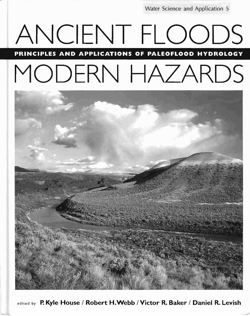
VVater Science and Appl ication 5

ANCIENT FLOODS PRINCIPLES AND APPLICATIONS OF PALEOFLOOD HYDROLOGY

MODERN HAZARDS

edited by ~ Kyle House / Robert H.Webb / Victor R. Baker / Daniel R. Levish

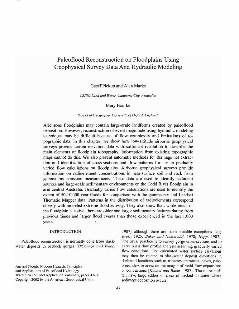
Paleoflood Reconstruction on Floodplains Using Geophysical Survey Data And Hydraulic Modeling

Geoff Pickup and Alan Marks

CSIRO Land and Water, Canberra City, Australia.

Mary Bourke

School ofGeography, University ofOxford, England.

Arid zone floodplains may contain large-scale landforms created by paleoflood deposition. However, reconstruction of event magnitude using hydraulic modeling techniques may be difficult because of flow complexity and limitations of to­pographic data. In this chapter, we show how low-altitude airborne geophysical surveys provide terrain elevation data with sufficient resolution to describe the main elements of floodplain topography. Jnformation from existing topographic maps cannot do this. We also present automatic methods for drainage net extrac­tion and identification of cross-sections and flow patterns for use in gradually varied flow calculations on floodplains. Airborne geophysical surveys provide information on radioelement concentrations in near-surface soil and rock from gamma ray emission measurements. These data are used to identifY sediment sources and large-scale sedimentary environments on the Todd River floodplain in arid central Australia. Gradually varied flow calculations are used to identifY the extent of 50-10,000 year floods for comparison with the gamma ray and Landsat Thematic Mapper data. Patterns in the distribution of radioelements correspond closely with modeled extreme flood activity. They also show that, while much of the floodplain is active, there are older and larger sedimentary features dating from previous times and larger flood events than those experienced in the last 1,000 years.

INTRODUCTION 1987] although there are some notable exceptions [e.g. Bretz, 1925; Baker and Nummedal, 1978; Hupp, 1987].

Paleoflood reconstruction is normally done from slack­ The usual practice is to survey gorge cross-sections and to water deposits in bedrock gorges [O'Connor and Webb, carry out a flow profile analysis assuming gradually varied

flow conditions. The calculated water surface elevations may then be related to slackwater deposit elevations in sheltered locations such as tributary entrances, caves, pale­

Ancient Floods, Modem Hazards: Principles omeanders or areas on the margin of rapid flow expansions and Applications of Paleoflood Hydrology or contractions [Kochel and Baker, 1987]. These areas of­Water Science and Application Volume 5, pages 47-60 ten have large eddies or areas of backed-up water where Copyright 2002 by the American Geophysical Union sediment deposition occurs.

47

48 PALEOFLOOD RECONSTRUCTION

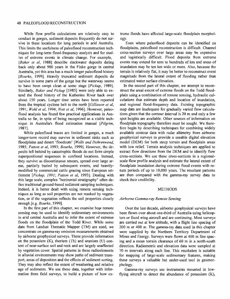
While flow profile calculations are relatively easy to conduct in gorges, sediment deposits frequently do not sur­vive in these locations for long periods in arid Australia. This limits the usefulness of paleoflood reconstruction tech­niques for long-tenn flood-frequency analysis and for stud­ies of extreme events in climate change. For example, [Baker et ai, 1988] describe slackwater deposits dating back only about 900 years in the Finke gorge in central Australia, yet this area has a much longer paleoflood history [Bourke, 1999]. Heavily truncated sediment deposits do survive in some parts of the gorge but the waterway seems to have been swept clean at some stage [Pickup, 1989]. Similarly, Baker and Pickup [1985] were only able to ex­tend the flood history of the Katherine River back over about 150 years. Longer time series have been reported from the tropical cyclone belt to the north [Gillieson et ai, 1991; Wohl et ai, 1994; Nott et ai, 1996]. However, paleo­flood analysis has found few practical applications in Aus­tralia so far, in spite of being recognized as a viable tech­nique in Australia's flood estimation manual [Pilgrim, 1987].

While paleoflood traces are limited in gorges, a much longer-tenn record may survive in sediment sinks such as floodplains and desert 'floodouts' [Wells and Dohrenwend, 1985; Patton et ai, 1993; Bourke, 1999]. However, the de­posits left behind by catastrophic floods do not fonn simple superpositional sequences in confmed locations. Instead, they survive as discontinuous smears, spread over large ar­eas, partially buried by subsequent events, and heavily­modified by commercial cattle grazing since European set­tlement [Pickup, 1991; Patton et ai, 1993]. Dealing with this large scale, complex "horizontal stratigraphy" often de­fies traditional ground-based sediment sampling techniques. Indeed, it is better dealt with using remote sensing tech­niques as long as soil properties are not masked by vegeta­tion, or if the vegetation reflects the soil properties closely enough [e.g. Bourke, 1999].

In the first part of this chapter, we examine h~ remote sensing may be used to identify sedimentary environments in arid central Australia and to infer the extent of extreme floods on the floodplain of the Todd River. While some data from Landsat Thematic Mapper (TM) are used, we concentrate on gamma-ray emission measurements obtained by airborne geophysical surveys. These provide infonnation on the potassium (K), thorium (Th) and uranium (U) con­tent of near-surface soil and rock and are largely unaffected by vegetation cover. Spatial patterns in these radioelements in alluvial environments may show paths of sediment trans­port, areas of deposition and the effects of sediment sorting. They may also reflect the extent of weathering and relative age of sediments. We use these data, together with infor­mation from field surveys, to build a picture of how ex­

treme floods have affected large-scale floodplain morphol­ogy.

Even where paleoflood deposits can be identified on floodplains, paleoflood reconstruction is difficult. Channel cross-section surveys over large areas may be expensive and logistically difficult. Flood deposits from extreme events may extend for tens to hundreds of km and areas of inundation may be ten km wide or more. Also, because the terrain is relatively flat, it may be better to reconstruct event magnitude from the lateral extent of flooding rather than estimated water surface elevation.

In the second part of this chapter, we attempt to recon­struct the areal extent of extreme floods on the Todd flood­plain using a combination of remote sensing, hydraulic cal­culations that estimate depth and location of inundation, and regional flood-frequency data. Existing topographic map data are inadequate for gradually varied flow calcula­tions given that the contour interval is 20 m and only a few spot heights are available. Other sources of infonnation on floodplain topography therefore must be sought. We there­fore begin by describing techniques for combining widely available contour data with radar altimetry from airborne geophysical surveys to provide a useable digital elevation model (DEM) for both steep terrain and floodplain areas with low relief. Terrain analysis techniques are applied to extract flow directions from the DEM and to identify flow cross-sections. We use these cross-sections in a regional­scale flow profile analysis and estimate the lateral extent of floodplain inundation during extreme flood events with re­turn periods of up to 10,000 years. The resultant patterns are then compared with the gamma-ray survey data to check their credibility.

METHODS

Airborne Gamma-ray Remote Sensing

Over the last decade, airborne geophysical surveys have been flown over about one-third of Australia using helicop­ters or fixed wing aircraft and are continuing. Most surveys are carried out at low altitude, with a flight line spacing of 200 m or 400 m. The gamma-ray data used in this chapter were supplied by the Northern Territory Department of Mines and Energy. Surveys were flown at 400 m line spac­ing and a mean terrain clearance of 60 m in a north-south direction. Radiometric and elevation data were sampled at 70 m intervals along each line. This resolution is suitable for mapping of large-scale sedimentary features, making these surveys a valuable but under-used tool in geomor­phology.

Gamma-ray surveys use instruments mounted in low­flying aircraft to detect the abundance of potassium (K),

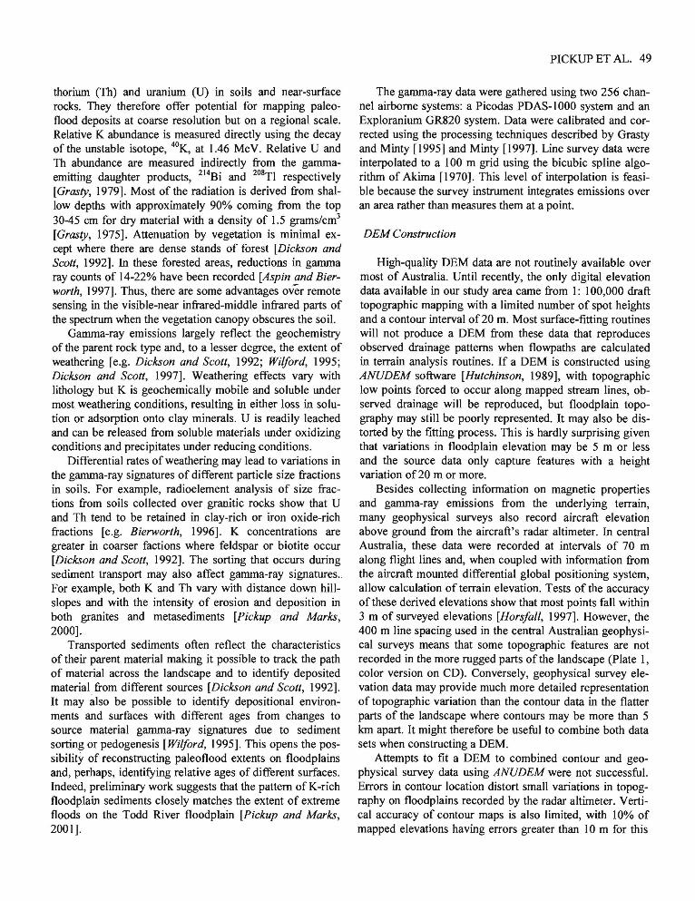
thorium (Th) and uraniwn (U) in soils and near-surface rocks. They therefore offer potential for mapping paleo­flood deposits at coarse resolution but on a regional scale. Relative K abundance is measured directly using the decay of the unstable isotope, 4OK, at 1.46 MeV. Relative U and Th abundance are measured indirectly from the gamma­emitting daughter products, 214Bi and 20sTI respectively [Grasty, 1979]. Most of the radiation is derived from shal­low depths with approximately 90% coming from the top 30-45 em for dry material with a density of 1.5 grams/cm3

[Grasty, 1975]. Attenuation by vegetation is minimal ex­cept where there are dense stands of forest [Dickson and Scott, 1992]. In these forested areas, reductions in gamma ray counts of 14-22% have been recorded [Aspin and Bier­worth, 1997]. Thus, there are some advantages over remote sensing in the visible-near infrared-middle infrared parts of the spectrwn when the vegetation canopy obscures the soil.

Gamma-ray emissions largely reflect the geochemistry of the parent rock type and, to a lesser degree, the extent of weathering [e.g. Dickson and Scott, 1992; Wilford, 1995; Dickson and Scott, 1997]. Weathering effects vary with lithology but K is geochemically mobile and soluble under most weathering conditions, resulting in either loss in solu­tion or adsorption onto clay minerals. U is readily leached and can be released from soluble materials under oxidizing conditions and precipitates under reducing conditions.

Differential rates of weathering may lead to variations in the gamma-ray signatures of different particle size fractions in soils. For example, radioelement analysis of size frac­tions from soils collected over granitic rocks show that U and Th tend to be retained in clay-rich or iron oxide-rich fractions [e.g. BielWorth, 1996]. K concentrations are greater in coarser factions where feldspar or biotite occur [Dickson and Scott, 1992]. The sorting that occurs during sediment transport may also affect gamma-ray signatures. For example, both K and Th vary with distance down hill­slopes and with the intensity of erosion and deposition in both granites and metasediments [Pickup and Marks, 2000].

Transported sediments often reflect the characteristics of their parent material making it possible to track the path of material across the landscape and to identifY deposited material from different sources [Dickson and Scott, 1992]. It may also be possible to identifY depositional environ­ments and surfaces with different ages from changes to source material gamma-ray signatures due to sediment sorting or pedogenesis [Wilford, 1995]. This opens the pos­sibility of reconstructing paleoflood extents on floodplains and, perhaps, identifYing relative ages of different surfaces. Indeed, preliminary work suggests that the pattern ofK-rich floodplain sediments closely matches the extent of extreme floods on the Todd River floodplain [Pickup and Marks, 2001].

PICKUP ET AL. 49

The gamma-ray data were gathered using two 256 chan­nel airborne systems: a Picodas PDAS-IOOO system and an Exploraniwn GR820 system. Data were calibrated and cor­rected using the processing techniques described by Grasty and Minty [1995] and Minty [1997]. Line survey data were interpolated to a 100 m grid using the bicubic spline algo­rithm of Akima [1970]. This level of interpolation is feasi­ble because the survey instrwnent integrates emissions over an area rather than measures them at a point.

DEM Construction

High-quality DEM data are not routinely available over most of Australia. Until recently, the only digital elevation data available in our study area came from 1: 100,000 draft topographic mapping with a limited number of spot heights and a contour interval of20 m. Most surface-fitting routines will not produce a DEM from these data that reproduces observed drainage patterns when flowpaths are calculated in terrain analysis routines. If a DEM is constructed using ANUDEM software [Hutchinson, 1989], with topographic low points forced to occur along mapped stream lines, ob­served drainage will be reproduced, but floodplain topo­graphy may still be poorly represented. It may also be dis­torted by the fitting process. This is hardly surprising given that variations in floodplain elevation may be 5 m or less and the source data only capture features with a height variation of20 m or more.

Besides collecting information on magnetic properties and gamma-ray emissions from the underlying terrain, many geophysical surveys also record aircraft elevation above ground from the aircraft's radar altimeter. In central Australia, these data were recorded at intervals of 70 m along flight lines and, when coupled with information from the aircraft mounted differential global positioning system, allow calculation of terrain elevation. Tests of the accuracy of these derived elevations show that most points fall within 3 m of surveyed elevations [Horsfall, 1997]. However, the 400 m line spacing used in the central Australian geophysi­cal surveys means that some topographic features are not recorded in the more rugged parts of the landscape (Plate 1, color version on CD). Conversely, geophysical survey ele­vation data may provide much more detailed representation of topographic variation than the contour data in the flatter parts of the landscape where contours may be more than 5 km apart. It might therefore be useful to combine both data sets when constructing aDEM.

Attempts to fit a DEM to combined contour and geo­physical survey data using ANUDEM were not successful. Errors in contour location distort small variations in topog­raphyon floodplains recorded by the radar altimeter. Verti­cal accuracy of contour maps is also limited, with 10% of mapped elevations having errors greater than 10m for this

50 PALEOFLOOD RECONSTRUCTION

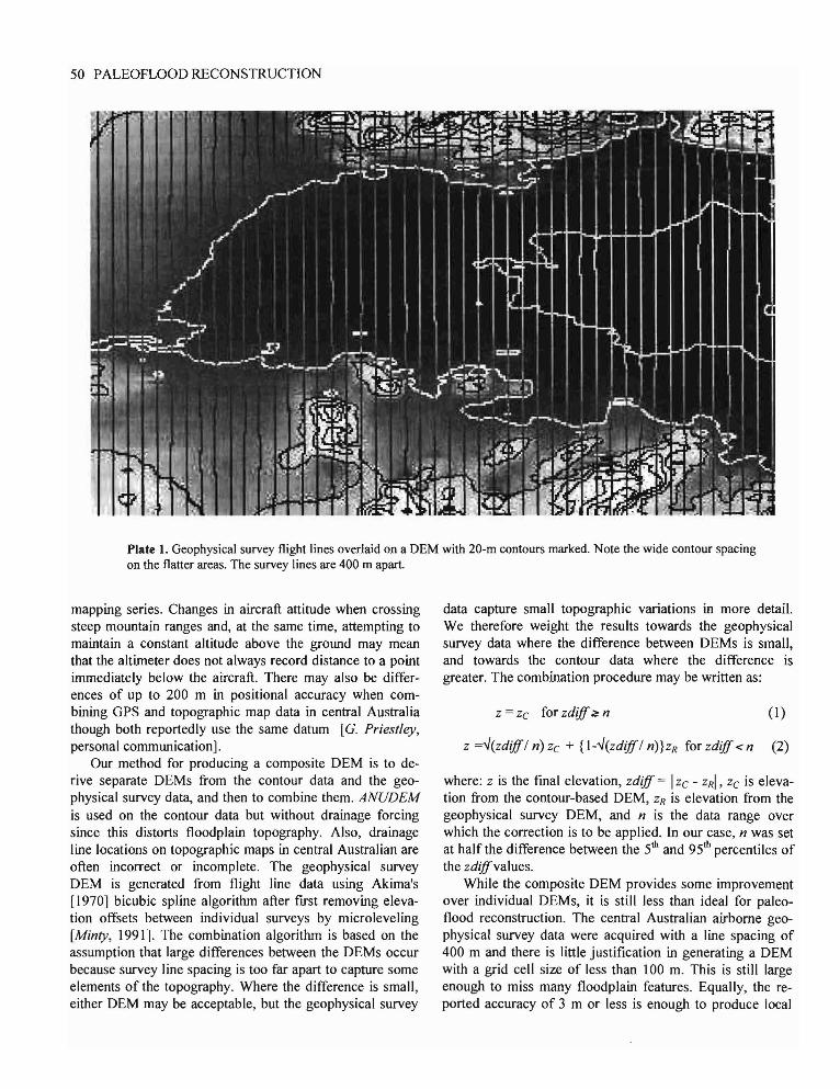
Plate I. Geophysical survey flight lines overlaid on a OEM with 20-m contours marked. Note the wide contour spacing on the flatter areas. The survey lines are 400 m apart.

mapping series. Changes in aircraft attitude when crossing steep mountain ranges and, at the same time, attempting to maintain a constant altitude above the ground may mean that the altimeter does not always record distance to a point immediately below the aircraft. There may also be differ­ences of up to 200 m in positional accuracy when com­bining GPS and topographic map data in central Australia though both reportedly use the same datum [G. Priestley, personal communication].

Our method for producing a composite DEM is to de­rive separate DEMs from the contour data and the geo­physical survey data, and then to combine them. ANUDEM is used on the contour data but without drainage forcing since this distorts floodplain topography. Also, drainage line locations on topographic maps in central Australian are often incorrect or incomplete. The geophysical survey DEM is generated from flight line data using Akima's [1970] bicubic spline algorithm after ftrst removing eleva­tion offsets between individual surveys by microleveling [Minty, 1991]. The combination algorithm is based on the assumption that large differences between the DEMs occur because survey line spacing is too far apart to capture some elements of the topography. Where the difference is small, either DEM may be acceptable, but the geophysical survey

data capture small topographic variations in more detail. We therefore weight the results towards the geophysical survey data where the difference between DEMs is small, and towards the contour data where the difference is greater. The combination procedure may be written as:

Z = Zc for zdijf:i? n (I)

z =...J(zdijfl n) Zc + {l-...J(zdijfl n)}zR for zdijf < n (2)

where: z is the fmal elevation, zdijf = IZc - ZR! , Zc is eleva­tion from the contour-based DEM, ZR is elevation from the geophysical survey DEM, and n is the data range over which the correction is to be applied. In our case, n was set at half the difference between the 5th and 95 th percentiles of the zdijfvalues.

While the composite DEM provides some improvement over individual DEMs, it is still less than ideal for paleo­flood reconstruction. The central Australian airborne geo­physical survey data were acquired with a line spacing of 400 m and there is little justiftcation in generating aDEM with a grid cell size of less than 100 m. This is still large enough to miss many floodplain features. Equally, the re­ported accuracy of 3 m or less is enough to produce local

PICKUP ET AL. 51

errors in paleoflood reconstruction. In spite of these diffi­culties, we believe that it should be possible to reproduce the major features of many extreme floods and there is cur­rently no other source of low-cost topographic data in the area of interest.

Flow Computations on Floadplains

Flow profile analysis in the bedrock gorges is usually carried out by surveying a series of channel cross-sections and carrying out gradually varied flow calculations using a computer package such as HEC-2 [Hydrologic Engineering Center, 1982]. Sub-critical flow is assumed and the calcu­lations are carried out cross-section by cross-section in the upstream direction. Flow profile analysis on floodplains follows a similar procedure but if the source data come from a OEM, flow directions and channel locations must frrst be identified before extracting channel cross-section

-·data. Cross-sections must also be sorted so the calculations' proceed in the upstream direction in reaches where flow is sub-critical.

Several terrain analysis packages offer routines for cal­culation of slope and aspect, identification of flow direc­tions, downstream accumulation of contributing areas and, if necessary, pit removal from OEM data. We have used the routines in TNT MIPs [MicroImages, 1999]. These routines produce a pitless OEM and route flow down slopes and across flats using an algorithm which passes the flow from a given grid cell into a single downstream neighbour based on the steepest direction of flow. This provides a data layer in which contributing drainage area increases progressively downstream and allows sorting of cross-sections into down­stream or upstream sequences. Terrain analysis packages that use a dispersion approach and allow flow to be propor­tioned out among several downstream neighbors based on terrain curvature are unsuitable because downstream flow directions do not always result in progressively increasing drainage area.

The next step is to identify cross-section locations and to extract cross-section profiles. We frrst set a minimum drainage area that is used to defme the stream network. Grid cells with a drainage area that exceeds this minimum are classed as channel centreline locations and sorted by de­creasing drainage area. A second sorting pass orders chan­nel centreline grid cells with a similar drainage area on the basis of increasing elevation. The procedures arrange chan­nel centerline grid cells so that gradually varied flow calcu­lations may be carried out in the upstream direction using the standard step method [Chow, 1959]. The calculations begin by assuming uniform flow in locations where the channel intersects the OEM boundary or where the channel terminates in a lake or floodout. Slopes for uniform flow calculations are taken from terrain analysis package results

or, in the case of terminating drainage lines, assigned a starting value. Channel cross-sections are identified by cal­culating mean flow direction at the centerline pixel and constructing orthogonals on each side. Mean flow direction is estimated based on a 10-20 grid cell moving window that is passed along each stream channel link. The gradually varied flow calculations produce a water depth, a friction slope, and the location of the inundated area. Water depths in grid cells between cross-sections are calculated by inter­polation.

The gradually varied flow algorithm, as described above, does not distinguish between active flow zones and areas of slackwater or backflow. These occur at expansions and contractions of the channel and of the flooded area. If the slackwater or backflow areas are included in the flow calculations, they will produce errors in cross-sectional area and mean velocity. We therefore conduct two passes through the calculations. The frrst pass makes no distinction between the active flow zone and other inundated areas but it does provide estimates of channel width. From this, we identify all constrictions along each channel. Active flow zones are then identified by restricting upstream and down­stream flow expansions to a user-specified angle (usually 15-45 degrees) on each side of the channel (CO Plate I). The gradually varied flow calculations are repeated with cross-sectional areas restricted to active flow zones. Inun­dated areas outside the active flow zone are also identified.

While this approach works reasonably well, there can be problems. No OEM is artifact-free, and in flat areas, small errors in flow direction can result in substantial misalign­ment of cross-sections. This is especially true with high­resolution OEMs, and it is sometimes better to re-sample to a lower spatial resolution before calculating channel aspect and setting the orthogonals that define each cross-section. A badly aligned cross-section may point upstream and down­stream rather than across a valley. Where this happens, water depths continuously increase in the downstream arm of the cross-section. In some cases, they may even cross a watershed, resulting in impossible flow depths and pre­venting the gradually varied flow calculations from con­verging on a solution.

We use one or more of three options to restrict or re­move this problem. Firstly, variations in flow direction may be smoothed to varying degrees by changing the size of the moving window. Secondly, a user-defined restriction may be placed on channel widths. This may involve limiting to­tal width or setting a maximum expansion angle for the in­undated area (usually 45-70 degrees, CO Plate 2). Thirdly, elevations in the cross-section may not fall below the chan­nel centerline elevation minus a threshold value that is set by the user. The most successful of these approaches is to apply a maximum expansion angle coupled with flow di­rection smoothing.

52 PALEOFLOOD RECONSTRUCTION

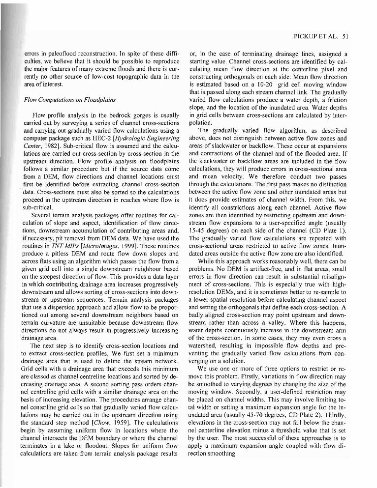
Plate 3. Radioelement concentrations in the MacDonnell Ranges and adjacent floodplains derived from an airborne gamma ray survey. Red is potassium, green is thorium and blue shows uranium. Area shown is 130 x 54 kIn. See text for an explanation of labels.

r (: )~~.~···V.,~ .---'"":wJ ~ .. ...~ ..... ,~~~:..,''~:'.,::' '."~~-' ..

,... . ,,~~. ' ,"

, .. > .."'~' ." . . • ' ..,·t· : ­"" d '.oJ '.,:" , .. : .. ', ..;r.Y..~ .,.- . " .' • ' / ..••'.,..

. ," ,: .r,' ,.,. ,:' .-.' ,I. '.'.'":_~'.'.:at \"",.;~~\f."_ . , .~ , - • "'., '~"'<J~~'; •. ., ....~ .;.. ~ ;,.. ,""- ",-_ ~ ,. ,...~.. ' ....ii:...~,- - ..... , " • v ..,\L"""""~""" - ~. ~. .

-~ . .' ;r • ",,""~r..~. y- ,.~"

..~.\

.'" '\. .. ,""",, '-', :', ".'. - . -. .. , . \<t<, '. ..: ,:S."::-:;i:..' .r -:~'.J'. ~k~;~4n?\ .~II>...'~,~ l~'.~;~.~,.~t.: ~. _'hI-" -~t-; '; .:- .....~...''-,. - ,,~.';<":• ,'-

,

..' " . " " ,,~' ,.. "".'; ...~ ,~ -; '.,:',:.i'. ,., ", ....~~.;' ~ "., •.~" .....- ~~ ~ )i,- '1:"' '. .,' ~ r '= ..6 '1.' ~ .. ,... . c

• #"_,',, ", 1,.....~~~~''f' ~. '~1:"""C" ~.~ ~\.,... ,"'j-"" ... '" "~" '" .:'~>:,.. .~~:.." •.' ";-" ,". ""::'~ \:'~ . .~ .. ,_ .. ._,-J'1 ~~~'~;~:'.w~~~~" 0-...<~::~". ",~,..•,1,.~',~~'. \......', ,.,_... ,. ''''. ,_:>.~ .. ::,,~,,~, '-' ,"#,,,, J. :,' ''J'" ,-1',.1~·" '"'...::i~'~''' :" '. 'I

_ ..... , "",i'-:; ~ " ..•..••~'g. " " •. ' " ,..... ,_,-:1 \",,, ~".' ,,..:;0-': 1.',F..<i:." , :.._,' • d " :', . :r;,.'i. . lot·· ,~""'T " =.. .'-' · - " .."'" .. .- _. . ,," l ... ,.. ,- ' • ..I"" , ~", ~- ,. ,~.....,.~I .• ' iii.. Y. ~ ~.,_.- .."' .' .·C' <~-' ·"1 '

'., ''-: ":.' ' .

'" .• ,_ ~ .~""', .. _ '.J' ~_ ;. "~.~/'o,¥" j " -.,., '

, ~. ~ •" ~ 1'J;ft". ..~.~:< c.1 ...'wY'r"~. ,

.~§\"....- .' .--".' '. """".

,;":L~ - -. ", '-.., .. ., •. I,

oJ - .

~ :~)t

.~ ~'-~ '

'"" .. • • . " '­ ' ~ .' ," ~

'\' i. .

'0­..,e '. ,

.....IJ(tt. ':""-'

....'J .. ~ ... ;., . ,.

~.""-.,, ... "" -..." .," ..... ",,-1. '. • .•• ,

. .:...; ;. ·1 . ~ .~~ .,-,

,.,.~., ,~ .~, fj':.:'~.'~'~ ,.­-~'" ".:;;. ~~t-· ~:. :jJ.'.,,' "~' .-1' . ':~

: .!'::'.' - ',' ..,"""':\, -"-;: ;.,-:~' .....:'<~.f(~

\ "'II

.,.,' : '., ,\ ~.:::. ... ..,:-,"- J<

. '-. . ' .f , .... I

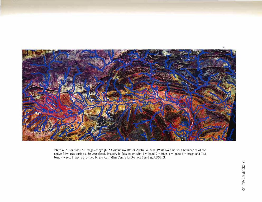
" '..J -Plate 4. A Landsat TM image (copyright * Commonwealth of Australia, June 1988) overlaid with boundaries of the active flow area during a 50·year flood. Imagery is false color with TM band 2 = blue, TM band 3 = green and TM band 4 = red. Imagery provided by the Australian Centre for Remote Sensing, AUSLIG.

.::!2 n i'" c -0 t'I1 -J » ~

v. w

54 PALEOFLOOD RECONSTRUCTION

REMOTE SENSING OF FLOODPLAIN CHARACTERlSTICS AND BEHAVIOR

The Todd River Drainage Basin

The Todd River is one the main ephemeral drainage sys­tems of central Australia (Plate 2, also on CD) [Bourke and Pickup, 1999]. Its headwaters lie in the central and eastern MacDonnell Ranges where its main tributaries occupy nar­row gorges (CD Plate 3). Beyond the ranges, the Todd oc­cupies a broad alluvial plain (CD Plate 4), ending in a large floodout between the dunes of the Simpson Desert (CD Plate 5). The area has a mean annual rainfall of 274 mm but experiences heavy rainfalls when influxes of moist tropical air destabilise the predominantly high-pressure system of warm dry air. Indeed, there are examples of the mean an­nual rainfall being received in less than 24 hours.

Paleoflood records from bedrock gorges in the region extend back about 900 years [Pickup et ai, 1988]. How­ever, many large-scale fluvial features on the floodplains are older and result from much larger events [Pickup, 199\; Patton et al 1993; Bourke 1999]. The events in the 900­year record are also well below the envelope of maximum recorded discharges world wide for catchments of the same size [Gillieson et ai, 1991]. Dating of flood deposits on the Todd floodplain as far back as 27,000 BP suggests that the largest events occurred in the late Pleistocene and early to mid-Holocene [Bourke, 1999]. Floods of the last 2,000 years are generally smaller in the Todd although the last century has been an extremely active period during which three of the four largest events in the 900-year record from the Finke have occurred.

Gamma-ray Data

Plate 3 (also on CD) shows radioelement concentrations in soils and near-surface rocks in the study area with the image enhanced to emphasize alluvial rather than bedrock areas. The main features are:

• The radioelement-rich gneiss and granite core of the MacDonnell Ranges;

• The folded metamorphic and sedimentary rocks on the southern and eastern rringe of this core; and

• The southern floodplain systems, including Roe Creek, the Todd and Ross Rivers, and Giles Creek.

Extensive folding is apparent in the sedimentary rocks that form a series of strike ridges developed on eroded anti­clines and synclines. Transported sediment can be seen ex­tending outwards rrom the mountain ranges on the southern floodplain systems. Indeed, some sediment can be tracked for long distances and gradual changes in their radio­element content observed.

The southern floodplain systems contain several major features. The Owen Springs area, which is bordered by the Hugh River in the west, is a relatively flat alluvial and lime­stone plain with extensive caliche deposits and a dis­continuous dust mantle. The area has experienced substan­tial soil erosion since European settlement and much of the transported material has accumulated in a series of shallow washes and floodouts. This material is dark red-brown in colour on the image, indicating low radioelement concen­trations but with K dominant. The exposed limestone, cali­che and derived soils are green in colour, indicating rela­tively high concentrations of Th.

The shallow washes of Owen Springs (marked A on Plate 3) are bordered in the east by the radioelement-rich floodplain deposits of Roe Creek. This material is derived from the gneiss and granite core of the MacDonnell Ranges (B on Plate 3). The Roe Creek floodplain (C on Plate 3) sharply truncates the Owen Springs floodouts, suggesting that these drainages have been blocked off or backed up (CD Plate 6). This may have occurred because more sedi­ment is coming down Roe Creek than from the Owen Springs area where the washes are choked by trees and shrubs. It is also possible that extreme floods are involved, with ponded water covering much of the Todd River flood­plain. For example, the dark area on the southern edge of the Todd floodplain is a large dune field (0 on Plate 3). A large embayment in this dune field at (E on Plate 3) con­tains an area of radioelement-rich sediment that appears to have come from Roe Creek and the Todd River. This sug­gests a large area of backflooding with ponded water and deposition of sediments. Sediments in this area are fme suggesting deposition from slow flowing or standing water. Floodplain surfaces closer to the active flow area of the Todd have large fields of low-amplitude gravel ripples.

The Todd floodplain extends eastwards to a narrow constriction created by the large dune field on its southern edge and several ridges on the north side that have blocked the passage of aeolian material, creating a discontinuous sand sheet. There is also a large floodout or alluvial fan (F on Plate 3) made up of sediments from the eastern Mac­Donnell Ranges that enter the floodplains immediately east of the gap. This may also partially block the gap and con­fme the Todd to a narrow reach on the southern side of the alluvial plain.

Upstream of the gap, the floodplain has two main ele­ments: active floodplain reaches (e.g., G on Plate 3); and older, large-scale, paleoflood landforms (H on Plate 3). The active floodplain reaches are white, bright yellow or bright green in colour, indicating a high radioelement content and sediment sources in the gneiss and granite areas. The paleo­flood landforms make up a series of slightly elevated sur­faces, often covered by large-scale sedimentary features such as linear bars, diversion channels and fields of

megaripples [Pickup, 1991] (CD Plates 7 and 8). These sur­faces may have been continuous but are now breached by the radioelement-rich, active floodplains of a number of minor tributaries of the Todd River that drain the gneiss and granite area, notably Emily Creek, Jessie Creek and Un­doolya Creek.

The paleoflood landfonns become progressively redder to the east, suggesting that sorting has occurred leading to progressively higher K content. This may reflect differences in the lithology of gneiss and granite source areas drained by tributary creeks from the north. There also appears to be more gravel present than on paleoflood landfonns further west, probably because sediment source areas are closer and there has been less downstream sorting.

Immediately west of the gap, the Ross River enters the Todd River floodplain (CD Plate 9). This system drains the eastern end of the gneiss and granite region of the Mac­Donnell Ranges ([ on Plate 3) as well as a large area of folded sedimentary rocks (J on Plate 3). The K-rich (red) channel sediments can be seen right through the Ross River gorge as it cuts through the sedimentary rocks (L on Plate 3). They also spread across the Ross River floodplain (M on Plate 3). The rest of the Ross River floodplain consists of large paleochannel systems and megaripple fields (CD Plate 10) [Patton et ai, 1993]. These are light green or yel­low in colour in the gamma ray image indicating a high content of all radioelements. This suggests that much of the sediment is derived from the gneiss and granite region of the eastern MacDonnell Ranges. The Ross River drains this area as well as the limestones and folded sedimentary rocks to the immediate north of the floodplain. Much of this ma­terial is extremely fine, suggesting that ponded water occu­pied the area long enough to allow large-scale deposition of silts and clays.

Giles Creek marks the eastem end of the Ross River floodplain and brings in darker, radioelement-poor sedi­ment derived from the sedimentary rocks (N on Plate 3). Reworked aeolian material also may be present since many of the valleys in this region contain extensive dunefields or sand sheets built from material blown in from the Simpson Desert immediately to the east. The Giles Creek sediments probably post-date and partly cover the paleochannel sys­tems of the Ross River floodplain and extend further south to eventually flood out into the Simpson Desert [Bourke, 1999]. Even so, Ross River sediments can be seen on the left hand side of the flood plain (0 on Plate 3) and extend right to the lower edge of the image. The changing colour of this material suggests mixing with Giles Creek sedi­ments.

PICKUP ET AL. 55

RECONSTRUCTION OF PALEOFLOOD EXTENTS ON THE TODD RIVER FLOODPLATN

Extent ofFlooding

We attempted to reconstruct the areal extent of flooding on the Todd River floodplain using the composite OEM, a regional flood frequency curve, and the flow computation techniques described above. The flood frequency curve was derived from gauging data in the Todd catchment [Mac­Queen, 1978], flood estimates for dam design [Jackson and Paige, J979], and data from a hydraulic model and sJack­water deposits from the Finke Gorge [Pickup et al 1988]. A Manning's n value of 0.125 [see Chow, J959 for typical floodplain roughness coefficients] was used in the hy­draulic calculations. Lateral expansion of the inundated area was limited to no more than 45 degrees from the main flow direction. Slackwater areas and backtlow zones were designated by restricting expansion of the active flow zone to an angle of 15 degrees from the main flow direction both upstream and downstream of flow contractions. These an­gles were derived from observed changes in channel and floodplain width (e.g. CD Plates J and 2). Maps showing the water depth in inundated areas and/or active flow zones for flood return periods of 50 to J0,000 years are shown in Plates 4 and 5 (also on CD).

The 50-year flood reconstruction was used as a test of how well the OEM reproduced observed drainages and tloodouts. Much of the drainage data on topographic maps in this area is of limited accuracy because well-defmed channels often do not exist and the shallow washes that re­place them are difficult to map. These features can be seen on Landsat TM imagery, particularly after heavy rains when vegetation response is greater along flow lines. We have therefore used Landsat TM imagery for June J988 as "truth" and overlaid the boundaries of the active flow zone for the 50-year flood for comparative purposes (Plate 4). This image was acquired approximately two months after a major flood that inundated much of the Todd floodplain and other parts of central Australia. This flood had a retum period of about 50 years on the Todd River upstream of Heavitree Gap. Its retum period for downstream reaches was probably less than this as rainfall declined to the east.

The TM image is false colour with the red areas indi­cating vigorous plant growth, usually where inundation has added extra soil moisture. The dark red areas are floodplain plant communities developed on sandy deposits with river redgums (Eucaplytus camaldulensis), and an understorey of buffel grass (Cenchrus ciliaris) or couch grass (Cynodon

56 PALEOFLOOD RECONSTRUCTION

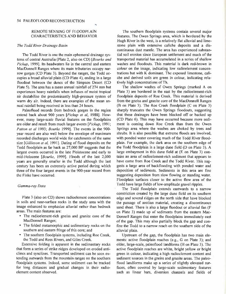
0-----------25m Plate 5. Depth of flooding in the study area during the 100-, 1000- and 10,000-year floods. White lines show boundary of inundated area. Colored area indicates water depths in m in active flow zone.

PICKUP ET AL. 57

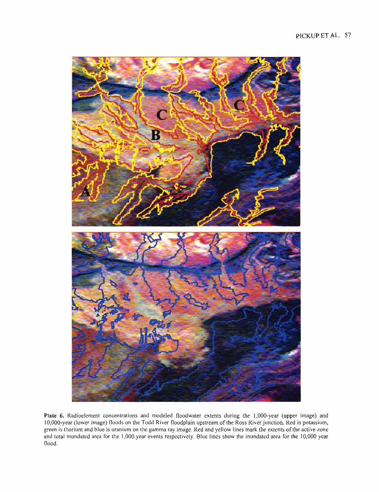
Plate 6. Radioelement concentrations and modeled floodwater extents during the 1,000-year (upper image) and IO,OOO-year (lower image) floods on the Todd River floodplain upstream of the Ross River junction. Red is potassium, green is thorium and blue is uranium on the gamma ray image. Red and yellow lines mark the extents of the active zone and total inundated area for the 1,000 year events respectively. Blue lines show the inundated area for the 10,000 year flood.

58 PALEOFLOOD RECONSTRUCTION

dactyfedon). Both grasses are introduced species and are aggressive coJonisers of floodplains and areas of sediment deposition. The pale red areas identifY floodplains with ei­ther buffel grass or ephemeral native grasses and forbs, but fewer trees. These areas have clay or clay-loam soils in many cases, indicating deposition of fmer material.

Comparison of the TM image and the active flow zones gives remarkably good results considering the quality of the elevation data and the fact that the DEM was fitted without forcing topographic lows on to mapped drainage lines. All charmel systems occur within the flooded area and most ar­eas of floodplain, as defmed by the vegetation, are identi­fied. Most of the dark red areas that lie outside the flooded area occur on aJluvial fans at the base of the mountain ranges or cover floodplains of streams with drainage areas below cut-off. In the few cases where the TM data and the flooded area are mismatched, the elevation differences are 2m or less.

Given the level of success in reproducing the 50-year flood, we have calculated the extent and depth of inun­dation for the 100-, 1,000- and 10,000-year floods using discharges from the regional flood frequency curve (Plate 5). The curve includes data from a slackwater deposit rec­ord extending back about 900 years so the value for the 1,000-year flood is close to being within historical limits. The 10,000-year flood discharge was obtained by extra­polation and represents an extreme condition for purposes of comparison rather than a defmitive value.

Many floodplain features are inundated by the 50-year event, suggesting that this floodplain is an active system. However, the small number of extreme flows in slackwater deposit record for this area suggests that change may be slow and that many features from earlier times should be preserved. Some areas remain above water during the flood. Many of these have been mapped as remnants of a Pleisto­cene floodplain surface [Bourke, 1999]. Other areas not in­undated include alluvial fans, dunefields and aeolian de­posits at the base of the mountain ranges. The fans would be active during most extreme events but have drainage ba­sins too small to be included in the gradually varied flow calculations. The upstream sections of some of the largest paleoflood bars are not submerged, even by the 1000-year flood. However, their downstream sections are covered by 5-10 m of water during this event. Most of the paleoflood bars would be inundated by the 1O,OOO-year event.

The water depths shown in Plate 5 were calculated as­suming steady-state flow conditions. This means that all streams experience peak flow simultaneously and that peak flows are maintained long enough for the whole system to achieve steady state. This is unlikely given the size of the Todd River drainage basin. Some water depths therefore may be exaggerated, particularly where flow constrictions raise water surface elevation in upstream floodplain

reaches. Water depths over the whole system may also be excessive in cases where localised storms generate extreme floods but infiltration into sandy riverbeds causes rapid de­pletion of flood '8ischarges as flood waves progress down­stream.

While many flood events in the slackwater deposit re­cord seem confmed to particular catchments, there is evi­dence for extreme rainfall events that occur across the re­gion. There are common dates for events in the Finke Gorge, Dashwood and Derwent Creeks, the Todd River, and the Ross River [Pickup et af, 1988; Patton et af 1993; Bourke, 1999; P. C. Patton, personal communication]. The affected area has a 100 km radius so these rainfall events must have been very large. They may also have lasted long enough for all systems to experience large flows simultane­ously although the occurrence of simultaneous flood peaks is unlikely. There is also anecdotal evidence for inundation of large areas in an early description of the site of Alice Springs in 1901:

"On the first survey flood marks were found which showed that the whole country to the north of the range must have been converted into a huge lake 15 feet deep and the blacks tell that before the white men came they had once to take refuge from the flood on the hill." [White, 1909, quoted by Kimber, 1996].

We conclude that the modeling results are reasonable for the regional scale events.

Comparison with Gamma-ray Imagery

The gamma-ray imagery provides information on flood­plain sedimentary environments that may be compared with modeled flow conditions to see whether there is any simi­larity. Before making this comparison, we have divided the area inundated by the 1000-year flood into active flow zones and areas of backwaterlslackwater since a different mix of particle sizes may be deposited in each. This process of sorting may affect radioelement content and give differ­ent gamma-ray signatures.

Plate 6 (also 00 CD) shows radioelement and flood ex­tent data for the Todd floodplain upstream of the Ross River junction for the 1,000- and 10,000-year events. On the Owen Springs drainage systems, the inundated areas correspond reasonably well with the red-brown areas on the gamma-ray image (A on Plate 6) for both events. On the Todd River and Roe Creek floodplains, there is some simi­larity between active flow zones for the I,OOO-year event and the green and yellow areas (B on Plate 6) but a better match was obtained with the 50-year flood (Plate 4). Most of these are mixed sand and gravel channel, avulsion and floodout deposits and are currently active to varying de­grees.

I

The backwaterlslackwater zones of the 1,000-year Todd floodplain correspond only partly with the red paleoflood features on the gamma-ray imagery (C on Plate 6). Many of these features lie outside the active flow zones and are only partly inundated by backwaterlslackwater. We suggest that they do receive fme sediments deposited during extreme events, but are older than the more radioelement rich active flow areas. Also, the linear bars and megaripples on some of the red paleoflood surfaces (CD Plates 7 and 10) imply active flow transporting sediment in quantity rather than standing water. The inundated area for the 10,000-year event covers most, but not all of these features, so they may result from an even larger flood. Further dating and strati­graphic investigations are needed to produce a flfill conclu­sion.

CONCLUSIONS

Terrain elevation data from airborne geophysical sur­veys can improve DEMs derived from topographic map in­formation to the extent that they may be used for regional­scale modeling of extreme flood events using gradually varied flow algorithms. These surveys also provide data on radioelement content of surface and near-surface soil and rock that may be used to identitY and map sedimentary en­vironments. In central Australia, these techniques allow us to identitY sediment sources and to discriminate between paleoflood deposits and sedimentary features associated with active floodplains.

Paleoflood modeling of the Todd River floodplain gen­erates patterns of inundation similar to those identified on Landsat TM imagery. The results also generate patterns that match sedimentary environments in the gamma-ray im­agery. This suggests that, while much of the floodplain has been active during the last 1,000 years, some floodplain features result from older and larger events. This conclu­sion matches the results of field studies that have identified floodplain landforms at several scales and concluded that

.the "largest features are the product of episodic and catas­trophic events.

Airborne geophysical survey data are becoming widely available and offer potential for regional scale investigation of both sediment transport and weathering patterns in a range of environments. They are deserving of much wider use by geomorphologists.

Acknowledgments. We are grateful to the Northern Territory Department of Mines and Energy for providing geophysical sur­vey data.

REFERENCES

Akima, H., A new method of interpolation and smooth curve fining based on local procedures, 1. Assoc. Computing Machinery. /7, 589-602, 1970.

PICKUP ET AL. 59

Aspin, SJ. and P.N. Bierworth, GIS analysis of the effects of forest biomass on gamma-radiometric images, Third National Forum on GIS in the Geosciences, Australian Geol. Surv. Org. Rec. 1997/36, 77-83, 1997.

Baker, V.R. and D. Nummedal, The Channeled Scabland, Planetary Geology Program, NASA, Washington, D.C., 186 pp, 1978.

Baker, V.R. and G. Pickup, Radiocarbon dating of flood events, Katherine Gorge, NT, Australia, Geology 13, 344-347, 1985.

Bierworth, P., Investigation of Airborne Gamma-Ray Images as a Rapid Mapping Tool for Soil and Land Degradation - Wagga Wagga, NSW. Australian Geol. Surv. Org. Rec. 1996/22, Australian Geological Survey Organisation, Canberra, 69pp, 1996.

Bourke, M.C.A., Fluvial Geomorphology and Paleofloods in Arid Central Australia, Ph.D. Thesis, Australian National Univ­ersity, Canberra, 208 pp, 1999.

Bourke, M. and G. Pickup, Variability of fluvial forms in the Todd River, Central Australia, in Varieties of Fluvial Form edited by A. Miller and A. Gupta, Wiley, Chichester, pp. 249­271,1999.

Bretz, J.H., The Spokane flood beyond the Channeled Scabland, 1. Geol, 33,97- 115,236-259, 1925.

Chow V.T. Open-Channel Hydraulics. McGraw-Hili Inc., New York, 680 pp, 1959.

Dickson, B.L. and K.M. Scott, Interpretation of Aerial Gamma­Ray Surveys, CSIRO Div. Exploration Geoscience Restricted Report, 301R, North Ryde, 144 pp, 1992.

Dickson, B.L. and K.M. Scott, Interpretation of aerial gamma-ray surveys - adding the geochemical factors, Australian Geol. Surv. Org. 1. Australian Geol. and Geophys., 17, 187-200, 1997.

Gillieson, D., D. Ingle Smith, and M. Ellaway, Flood history of the Limestone ranges in the Kimberley region, Western Australia, Appl Geog. I I, 105-123, 1991.

Grasty, R.L., Atmospheric absorption of 2.62 MeV gamma-ray photons emitted from the ground, Geophysics, 40, 1058-1065, 1975.

Grasty, R.L., Gamma-ray spectrometric methods in uranium exploration - theory and operational procedures, in Geophysics and Geochemistry in the Search for Metallic Ores, Geological Survey of Canada, Economic Geology Report 31, edited by P. J. Hood, pp. 147-161,1979.

Grasty, R.L. and B.R. Minty, A guide to the technical speci­fications for airborne gamma-ray surveys, Australian Geol Surv. Org. Record 1995/60, 89 pp, 1995.

Horsfall, K.R., Airborne magnetic and gamma-ray data acqui­sition, Australian Geological Survey Organisation Journal of Australian Geology and Geophysics 17,23-30, 1997.

Hupp, C. R., Plant ecological aspects of flood geomorphology and paleoflood history, in Flood Geomorphology, edited by V. R. Baker, K. C. Kochel and P. C. Patton, pp. 335-356, John Wiley, New York, 1987.

Hutchinson, M. F., A new method for gridding elevation and stream line data with automatic removal of pits, Journal of Hydrology, 106, 211-232, 1989.

Hydrologic Engineering Center, HEC-2 Water Surface Profiles User Manual, US Army Corps Of Engineers, Davis, Cali­fornia, 1982.

)

60 PALEOFLOOD RECONSTRUCTION

Jackson, D. and D. Paige, Alice Springs Recreational Dam Hydrology Report, Northern Territory of Australia Department of Transport and Works Hydrology Division, Darwin, 50pp, 1979.

Kimber, RG., The dynamic century before the Hom Expedition: a speculative history, in Exploring Central Australia: Society. the Environment and the Horn Expedition, edited by S. R Morton and OJ. Mulvaney, Beatty and Sons, Chipping Norton, Surrey, pp. 99- I02, 1996.

Kochel, R.C. and V.R. Baker, Paleoflood analysis using slack­water deposits, in Flood Geomorphology, edited by V.R Baker, R.C. Kochel and P.c. Patton, Wiley Interscience, New York, pp. 357-376,1987.

MacQueen, A.D., Flood Frequency in Central Australia, a Regional Model, Northern Territory of Australia Dept. Transport and Works Hydrology Division, Darwin, 1978.

Microimages Inc., TNT Mips Reference Manual, Lincoln, Nebraska, 1999.

Minty, B.R.S., Simple microlevelling for aeromagnetic data, bplor. Geophys., 22,59 J-592, 1991.

Minty, B.R.S., Fundamentals of airborne gamma-ray spec­trometry, Australian Geo!. Surv. Org. 1. Australian Geo!. and Geophys., 17, 39-50, 1997.

Nott, J., D.M. Price, and E.A. Bryant, A 30,000-year record of extreme floods in tropical Australia from relict plunge-pool deposits. Implications for future climate change, Geophys. Res. Let., 23, 379-382,1996.

O'Connor, J.E. and R.H. Webb, Hydraulic modeling for paleo­tlood analysis, in Flood Geomorphology, edited by V.R. Baker, R.C. Kochel and P.C. Patton, Wiley, New York, pp. 393-402, 1988.

Patton, P.c., G. Pickup, and D.M. Price, Holocene paleofloods of the Ross River, Central Australia, Quat. Res., 40, 201-212, 1993.

Pickup, G., Paleoflood hydrology and estimation of the mag­nitude, frequency and areal extent of extreme floods - an Australian perspective, Civil Eng. Trans. Institution of Engineers, Australia, 253-263, 1989.

Pickup, G., V.R Baker, and G. Allan, History, Paleochannels and Paleofloods of the Finke River, central Australia, in Australian Fluvial Geomorphology, edited by R.F. Warner, Academic Press, Sydney, pp. 105-127, 1988.

Pickup, G., Event frequency and landscape stability on the floodplains of arid central Australia, Quat. Sci. Rev., 10, 463­473,1991.

Pickup, G. and A. Marks, IdentifYing large-scale erosion and deposition processes from airborne gamma radiometrics and digital elevation models in a weathered landscape, Earth Surf Proc. Landf, 25,535-557,2000.

Pickup, G. and A. Marks, Regional-scale sedimentation process models from airborne gamma-ray remote sensing and digital elevation data, Earth Surf Proc. Landf, 26, 273-29, 200 I.

Pilgrim, D. H., Australian Rainfall and Runoff. A Guide to Flood Estimation, Institution of Engineers, Australia, Barton, ACT, 374 pp, 1987.

Wells, S. G. and J.C. Dohrenwend, Relict sheet flood bed forms on late Quaternary alluvial fan surfaces in the southwestern United States, Geology, 13, 512-5 I6, 1985.

Wilford, J., Airborne gamma-ray spectrometry as a tool for assessing relative landscape activity and weathering devel­opment of regolith, including soils, Australian Geo!. Surv. Org. Research Newsletter, 22, 12-14, 1995.

Wohl, E.R., R.H. Webb, V.R Baker, and G. Pickup, Sedimentary flood records in bedrock canyons in the monsoonal region of Australia, Colorado State Univ. Wat. Resour. Pap., 107, 102 pp, 1994.

Geoff Pickup, CSIRO Land and Water, PO Box 1666, Canberra City, ACT 2601, Australia.

Alan Marks, CSIRO Land and Water, PO Box 1666, Canberra City, ACT 260 I, Australia.

Mary Bourke, School of Geography and the Environment, Uni­versity of Oxford, Mansfield Road, Oxford, OX I 3TB, Eng­land.