Embed Size (px)
Citation preview

arX
iv:1
111.
5511
v1 [
astr
o-ph
.GA
] 23
Nov
201
1Astronomy & Astrophysicsmanuscript no. VVV˙DR1 c© ESO 2018April 1, 2018
VVV DR1: The First Data Release of the Milky Way Bulge andSouthern Plane from the Near-Infrared ESO Public Survey VIS TA
Variables in the V ıa Lactea⋆
R. K. Saito1, M. Hempel1, D. Minniti1,2,3, P. W. Lucas4, M. Rejkuba5, I. Toledo6, O. A. Gonzalez5, J. Alonso-Garcıa1,M. J. Irwin7, E. Gonzalez-Solares7, S. T. Hodgkin7, J. R. Lewis7, N. Cross8, V. D. Ivanov9, E. Kerins10,
J. P. Emerson11, M. Soto12, E. B. Amores13,14, S. Gurovich15, I. Dekany1, R. Angeloni1, J. C. Beamin1, M. Catelan1,N. Padilla1,16, M. Zoccali1,17, P. Pietrukowicz18, C. Moni Bidin19, F. Mauro19, D. Geisler19, S. L. Folkes20,
S. E. Sale1,20, J. Borissova20, R. Kurtev20, A. V. Ahumada9,21,22, M. V. Alonso15,21, A. Adamson23, J. I. Arias12,R. M. Bandyopadhyay24, R. H. Barba12,25, B. Barbuy26, G. L. Baume27, L. R. Bedin28, A. Bellini29, R. Benjamin30,
E. Bica31, C. Bonatto31, L. Bronfman32, G. Carraro9, A. N. Chene19,20, J. J. Claria21, J. R. A. Clarke20, C. Contreras4,A. Corvillon1, R. de Grijs33,34, B. Dias26, J. E. Drew4, C. Farina27, C. Feinstein27, E. Fernandez-Lajus27,R. C. Gamen27, W. Gieren19, B. Goldman35, C. Gonzalez-Fernandez36, R. J. J. Grand37, G. Gunthardt21,
N. C. Hambly8, M. M. Hanson38, K. G. Hełminiak1, M. G. Hoare39, L. Huckvale10, A. Jordan1, K. Kinemuchi40,A. Longmore41, M. Lopez-Corredoira42,43, T. Maccarone44, D. Majaess45, E. L. Martın46, N. Masetti47,
R. E. Mennickent19, I. F. Mirabel48,49, L. Monaco9, L. Morelli29, V. Motta20, T. Palma21, M. C. Parisi21, Q. Parker50,51,F. Penaloza20, G. Pietrzynski18,19, G. Pignata52, B. Popescu38, M. A. Read8, A. Rojas1, A. Roman-Lopes12,
M. T. Ruiz32, I. Saviane9, M. R. Schreiber20, A. C. Schroder53,54, S. Sharma20,55, M. D. Smith56, L. Sodre Jr.26,J. Stead39, A. W. Stephens57, M. Tamura58, C. Tappert20, M. A. Thompson4, E. Valenti5, L. Vanzi16,59, N. A. Walton7,
W. Weidmann21, and A. Zijlstra10
(Affiliations can be found after the references)
Received ; Accepted
ABSTRACT
Context. The ESO Public Survey VISTA Variables in the Vıa Lactea (VVV) started in 2010. VVV targets 562 sq. deg in the Galactic bulge andan adjacent plane region and is expected to run for∼ 5 years.Aims. In this paper we describe the progress of the survey observations in the first observing season, the observing strategy and quality of the dataobtained.Methods. The observations are carried out on the 4-m VISTA telescope in theZY JHKs filters. In addition to the multi-band imaging the variabilitymonitoring campaign in theKs filter has started. Data reduction is carried out using the pipeline at the Cambridge Astronomical Survey Unit. Thephotometric and astrometric calibration is performed via the numerous 2MASS sources observed in each pointing.Results. The first data release contains the aperture photometry and astrometric catalogues for 348 individual pointings in theZY JHKs filterstaken in the 2010 observing season. The typical image quality is ∼ 0.′′9 − 1.′′0. The stringent photometric and image quality requirements of thesurvey are satisfied in 100% of theJHKs images in the disk area and 90% of theJHKs images in the bulge area. The completeness in theZ andY images is 84% in the disk, and 40% in the bulge. The first seasoncatalogues contain 1.28× 10⁸ stellar sources in the bulge and 1.68× 10⁸ inthe disk area detected in at least one of the photometric bands. The combined, multi-band catalogues contain more than 1.63× 10⁸ stellar sources.About 10% of these are double detections due to overlapping adjacent pointings. These overlapping multiple detectionsare used to characterisethe quality of the data. The images in theJHKs bands extend typically∼ 4 mag deeper than 2MASS. The magnitude limit and photometricqualitydepend strongly on crowding in the inner Galactic regions. The astrometry forKs = 15− 18 mag hasrms ∼ 35− 175 mas.Conclusions. The VVV Survey data products offer a unique dataset to map the stellar populations in the Galactic bulge and the adjacent planeand provide an exciting new tool for the study of the structure, content and star formation history of our Galaxy, as well as for investigations ofthe newly discovered star clusters, star forming regions inthe disk, high proper motion stars, asteroids, planetary nebulae, and other interestingobjects.
Key words. Galaxy: bulge – Galaxy: disk – Galaxy: stellar content – Stars: abundances – Infrared: stars – Surveys
1. Introduction
The VISTA Variables in the Vıa Lactea (VVV) Survey is map-ping 562 square degrees in the Galactic bulge and the south-ern disk in the near-infrared (Minniti et al. 2010). The VVV
Send offprint requests to: R. K. Saito: [email protected]⋆ Based on observations taken within the ESO VISTA Public Survey
VVV, Programme ID 179.B-2002
Survey gives near-IR multi-colour information in five passbands:Z (0.87µm), Y (1.02µm), J (1.25µm), H (1.64µm), andKs(2.14µm), as well as time coverage spanning over 5 years, thatwill complement past/recent, current and upcoming surveys suchas 2MASS, DENIS, GLIMPSE-II, VPHAS+, MACHO, OGLE,EROS, MOA, PLANET, and GAIA.
VVV is an ESO Public Survey, i.e., the observational rawdata are made available to the astronomical community imme-
2 Saito et al.: VVV DR1
diately, whereas the reduced data will be published once a yearin a Data Release through ESO. This paper describes and char-acterises the first data release (DR1) of the VVV Survey. Somefirst results of the VVV Survey based on early science imagestaken in the bulge and disk fields are highlighted in Saito et al.(2010) and Catelan et al. (2011).
The preparatory phase for the VVV Survey started in 2006,with the first test observations obtained in October 2009. Regularoperations started with the first survey observations in February2010. The data collected during the first year of observationsuntil October 2010 are the subject of this public release. Oursurvey is planned to be carried out for 5 years, and we expect toproduce yearly accumulated data releases.
The VVV Survey is foremost a variability study of the in-ner regions of the Milky Way (Minniti et al. 2010), but will alsocomplement the existing 2MASSJHK photometry (Cutri et al.2003), extending to much fainter limits while adding two ad-ditional filters (ZY), and providing time domain informationuseful for variability and proper motion studies. In particular,the higher resolution of the VVV data represents a huge ad-vantage in crowded fields in relation to previous near-IR sur-veys such as 2MASS and DENIS (Epchtein et al. 1994), wherethe single-epoch photometry was confusion-limited, reachingKs ∼ 14.3 mag. The limiting magnitude of the VVV datausing aperture photometry isKs ∼ 18.0 mag in most fields.Even in the innermost fields (|b| ≤ 1◦) the VVV SurveyreachesKs ∼ 16.5 mag, at least a magnitude deeper than theIRSF/SIRIUS Survey of the Galactic Centre (Nagayama et al.2003; Nishiyama et al. 2006, 2009).
The VVV Survey was designed to complement the UKIDSS-GPS (Lucas et al. 2008), VPHAS+ (see Arnaboldi et al. 2007),and the GLIMPSE-II surveys (Benjamin et al. 2003). TheUKIDSS-GPS is mapping|b| < 5◦ in Galactic latitude in thenorthern plane for 3 epochs, while VPHAS+ also observes theGalactic plane in the optical and Hα using the ESO VLT SurveyTelescope (VST).
GLIMPSE-II survey images the central±10◦ of the plane in4 bands with IRAC. VVV provides variability information forthe overlap region, supporting studies of the content and distri-bution of stars, stellar populations, and interactions of the strongnuclear wind with the ambient ISM above and below the nu-cleus, as well as the rate and location of current star formation.
Multiband Spitzer public surveys with IRAC (mid-IR at3.6µm, 4.5µm, 5.6µm and 8.0µm) and MIPS (far-IR, 23.7µm,71.4µm weighted average wavelength), respectively, cover themid-plane (|b| < 1◦) at 65◦ < l < 10◦ and−10◦ < l < −65◦. Thesouthern half of these surveys overlaps with the VVV disk area,allowing the detection and characterisation of star formation re-gions and to probe the structure of the inner disk of the Galaxy.In optically obscured regions the IRAC data complement boththe VVV Survey and the VST/VPHAS+ by tracing the influenceof the most massive stars on star formation.
In addition, we complement the existing bulge microlens-ing surveys such as MACHO (Alcock et al. 2000) and OGLE(Udalski et al. 1993), which observe in optical bands, with lim-ited or no colour information. These surveys mostly concentrateon regions of low extinction. VVV will provide useful variabilityinformation for the overlap regions.
The data are of excellent quality in general, and only a smallfraction did not pass our quality controls and had to be reac-quired. These DR1 data have passed all the initial quality con-trols as performed by the survey team in collaboration with the
Cambridge Astronomical Survey Unit (CASU)1. We checkedimage defects, telescope problems, seeing, zero point, magni-tude limit, ellipticity and airmass, for instance. However, it isimportant to stress that the data quality and calibrations will im-prove with subsequent data releases.
Here we will address the general information for the commu-nity, e.g., on the survey area and strategy, data quality, progressin the observations, published source lists, as well as examplesof specific applications. In addition, the data, proceduresand ad-ditional information are available through the ESO Archive2, theVVV Survey Science Team homepage3, CASU, and through theVISTA Science Archive (VSA) webpage4.
This paper is organized as follows:Section 2 describes the area coverage and the observations
with VISTA as well as the data processing. Section 3 describesthe photometric quality (limits, accuracy), as well as complete-ness. Section 4 discusses a comparison with 2MASS. Section 5presents a comparison between the VVV DR1 (aperture) cata-logues and PSF photometry. Section 6 describes the astrometricdata quality. Section 7 presents density maps for the bulge anddisk fields. Section 8 describes a suitability test of the DR1datafor difference image analysis.
The final section summarizes and presents our conclusions,including important caveats regarding this DR1, and futureim-provements to be implemented in DR2. Finally, the VVV tilecoordinates are listed in the Appendix.
2. Survey Area and Observations
2.1. Telescope and Instrument
The telescope used to carry out the VVV Survey is VISTA(Visible and Infrared Survey Telescope for Astronomy), a4-m class wide-field telescope with a single instrument,VIRCAM (VISTA InfraRed CAMera; Dalton et al. 2006;Emerson & Sutherland 2010), located on its own peak at ESO’sCerro Paranal Observatory in Chile, about 1500m away fromthe VLT. Its primary mirror has a diameter of 4.1m, providingaf /3.25 focal ratio at the Cassegrain focus where the instrumentis mounted. The secondary mirror has a 1.24m diameter. Thestart of survey operations of the telescope was on April 1, 2010,but most VISTA surveys, including VVV, started collecting sci-ence observations a few months earlier, in parallel with thelastphases of the scientific performance verification and operationsfine-tuning performed by Paranal Observatory staff. During thefirst year of operations the mirrors were coated with silver,whichis optimized for near-IR observations.
With 1.64 deg diameter VIRCAM offers the largest un-vignetted field of view in the near-IR regime on 4-m classtelescopes. It is equipped with 16 Raytheon VIRGO 2048×2048 pixels2 HgCdTe science detectors, with 0.′′339 averagepixel scale. Each individual detector therefore covers∼ 694×694 arcsec2 on the sky. The achieved image quality (includingseeing) is better than∼ 0.′′6 on axis. The image quality distor-tions are up to about 10% across the wide field of view. The de-tectors are arranged in a 4× 4 array, with large spacings of 90%and 42.5% of the detector size along theX andY axes, respec-tively. A single pointing, called a pawprint, covers 0.59 sq. deg,and provides partial coverage of the field of view. By combining
1 http://casu.ast.cam.ac.uk/vistasp/2 http://www.eso.org/sci/archive.html3 http://vvvsurvey.org4 http://horus.roe.ac.uk/vsa/index.html

Saito et al.: VVV DR1 3
Fig. 1. Transmission curves for the five broad band filters presentat the VIRCAM:Z, Y, J, H andKs, compared with the typicalatmospheric transmission profile for airmass= 1.0 and 1.0 mmwater vapour. The effective wavelengths for all filters are listedin Table 1.
6 pawprint exposures with appropriate offsets a contiguous cov-erage of a field is achieved with at least 2 exposures per pixelexcept at two edges. In all VISTA observations such a field iscalled a tile and covers a 1.64 sq. deg field of view. Throughoutthis paper we will use a tile as the individual exposure.
VIRCAM has four additional optical CCDs, two for guidingand two for active optics. For exposures longer than∼ 40 secthe active optics is run in parallel mode with the observations.Due to VVV’s very short individual exposures of (see Sec. 2.3)the active optics correction is only performed every∼ 30 minor after a larger offset. This, combined with the need to surveythe area fast (hence minimizing the overheads for more frequentactive optics corrections), and typical seeing on Paranal limitsthe image quality obtained for the survey data to typically∼ 0.9−1.0 arcsec (see Sec. 2.4).
VIRCAM is equipped with 5 broad-band filters (Z, Y, J, H,andKs) and two narrow-band filters centred at 0.98 and 1.18µm.The VVV Survey uses all 5 broad band filters spanning from0.84 to 2.5µm. Their effective wavelengths and relative extinc-tions are given in Table 1, while the transmission curves areshown in Fig. 1, compared to a typical atmospheric transmissionprofile for airmass 1.0 and 1mm water vapour in the atmosphere.
For more details about the telescope and instrumentwe refer to the VIRCAM instrument web pages5, and theVISTA/VIRCAM User Manual (Ivanov & Szeifert 2009).
2.2. Survey area
The VVV Survey area consists of 348 tiles, 196 tiles in the bulgeand 152 in the disk area. These two components were planned tocover 520 sq. deg, as follows: (i) the VVV bulge survey area cov-ers 300 sq. deg between−10◦ ≤ l ≤ +10◦ and−10◦ ≤ b ≤ +5◦;and (ii) the VVV disk survey area covers 220 sq. deg between295◦ ≤ l ≤ 350◦ and−2◦ ≤ b ≤ +2◦. However, in order tomaximize the efficiency of the tilling process (see Section 2.3),the Survey Area Definition Tool (SADT; Hilker et al. 2011) pro-duced some shifts at the edges of the survey area, and as the re-
5 http://www.eso.org/sci/facilities/paranal
/instruments/vircam/
Table 1. Effective wavelengths for the VISTA filter set usedin the VVV observations and the relative extinction for eachfilter based on the Cardelli et al. (1989) extinction law (fromCatelan et al. 2011).
Filter λeff(µm) AX/AV AX/E(B − V)
Z 0.878 0.499 1.542Y 1.021 0.390 1.206J 1.254 0.280 0.866H 1.646 0.184 0.567Ks 2.149 0.118 0.364
Table 2. VVV Survey completion in the 2010 season.
Tile Completed Total Completiontype Tile Tiles percentage
Bulge
JHKs 188 196 95%ZY 78 196 40%
Variability 113 5× 196 12%
Disk
JHKs 152 152 100%ZY 128 152 84%
Variability 547 5× 152 72%
sult an area of∼562 sq. deg (42 sq. deg larger) was observed.Thus, the observed area is within−10.0◦ . l . +10.4◦ andwithin −10.3◦ . b . +5.1◦ in the bulge, and 294.7◦ . l . 350.0◦
and−2.25◦ . b . +2.25◦ in the disk. The VVV Survey area andtile numbering are shown in Fig. 2, while the list of all tile cen-tres in Equatorial and Galactic coordinates is given in Table A.1.The tile names start with “b” for bulge and “d” for disk tiles,followed by the numbering shown in Fig. 2.
While the whole area was observed in theJHKs, 95% ofthese tiles satisfy the stringent photometric and image qualityparameters and are classified as completed. In theZY bands thecompletion is somewhat lower, with 59% completed tiles. Thetiles completed in the first season (until October 26, 2010) canbe seen in Figs. 3, 4 and 5, respectively forZY, JH, and Ks.Figure 5 also includes the tiles with at least one epoch observedduring the variability campaign in theKs band.
In the first season of the variability campaign 22 tiles in thedisk area had 5Ks epochs taken, while the majority had oneor more additionalKs epochs completed. The completion ratesindividually for the bulge and disk areas are given in Table 2.Table A.1 states for each tile whether the observations in a givenfilter are completed, and how many additionalKs epochs wereobtained until October 26, 2010.
Figure 6 shows cumulative distributions of image quality andairmass for the observed tiles in the 2010 season. The medianimage quality in theJ, H and Ks filters is better than 0.′′9 asmeasured on combined tile images, while it is close to 1.′′0 fortheZ andY filters.

4 Saito et al.: VVV DR1
10 0 350 340 330 320 310 300Galactic Longitude [deg]
-10
-8
-6
-4
-2
+0
+2
+4
Gal
actic
Lat
itude
[deg
]
201 202 203 204 205 206 207 208 209 210 211 212 213 214
215 216 217 218 219 220 221 222 223 224 225 226 227 228
229 230 231 232 233 234 235 236 237 238 239 240 241 242
243 244 245 246 247 248 249 250 251 252 253 254 255 256
257 258 259 260 261 262 263 264 265 266 267 268 269 270
271 272 273 274 275 276 277 278 279 280 281 282 283 284
285 286 287 288 289 290 291 292 293 294 295 296 297 298
299 300 301 302 303 304 305 306 307 308 309 310 311 312
313 314 315 316 317 318 319 320 321 322 323 324 325 326
327 328 329 330 331 332 333 334 335 336 337 338 339 340
341 342 343 344 345 346 347 348 349 350 351 352 353 354
355 356 357 358 359 360 361 362 363 364 365 366 367 368
369 370 371 372 373 374 375 376 377 378 379 380 381 382
383 384 385 386 387 388 389 390 391 392 393 394 395 396
1 2 3 4 5 6 7 8 9 10 11 12 13 14 15 16 17 18 19 20 21 22 23 24 25 26 27 28 29 30 31 32 33 34 35 36 37 38
39 40 41 42 43 44 45 46 47 48 49 50 51 52 53 54 55 56 57 58 59 60 61 62 63 64 65 66 67 68 69 70 71 72 73 74 75 76
77 78 79 80 81 82 83 84 85 86 87 88 89 90 91 92 93 94 95 96 97 98 99 100 101 102 103 104 105 106 107 108 109 110 111 112 113 114
115 116 117 118 119 120 121 122 123 124 125 126 127 128 129 130 131 132 133 134 135 136 137 138 139 140 141 142 143 144 145 146 147 148 149 150 151 152
Fig. 2. VVV Survey area and tile numbering. The tile names start with“b” for bulge and “d” for disk tiles, followed by the numberingas shown in the figure. The centre coordinates for all VVV tiles are listed in Table A.1.
Fig. 3. The 5σ magnitude limits of the catalogues in theZ (top panel) andY bands (bottom panel). The colour scale is shown ineach case. The completeness of the DR1 can be also checked in the maps, where the missing tiles appear in black. Exposure timesin the bulge and disk fields are different (see Table 3), which contributes the disk fields to havedeeper photometry. Similar maps forJ, H andKs photometry, as well as for the variability campaign, are presented in Figs. 4 and 5.
2.3. Observing strategy
The first observations collected for the VVV Survey weretaken during the VISTA science verification period in October2009 when one field in the Galactic bulge atα=18:02:58.872,δ = −28:36:59.04 (J2000) was observed in theZYJHKs filters(called SV field). In addition to the nearly-simultaneous multi-band images of the SV field, 11Ks band exposures were takento test the variability observing strategy. To establish the neces-sary number of exposures for proper sky subtraction, dependingon crowding and number of resolved objects in the field, threeadditional tiles were observed in theKs band, two bordering di-
rectly on the SV field and one at an offset position≈1◦ south ofthe science target. Based on these early observations we adjustedthe observing strategy, which differs slightly between the bulgeand disk fields (i.e., with respect to exposure time, number of co-added exposures, and combination of tiles for sky subtraction).
Like all VISTA observations the VVV Survey is carried outin Service Mode. The basic observational unit is the so-calledOB (observation block). The multi-filter, single-epoch OBshavebeen split intoJHKs andZY OBs. The variability monitoringOBs have only single filter:Ks. OBs for two, three or four tileswere executed back-to-back to ensure that a sufficient number of

Saito et al.: VVV DR1 5
Fig. 4. The 5σ magnitude limits of the catalogues in theJ (top panel) andH bands (bottom panel). The notation is similar to thatpresented in Fig. 3.
Table 3. Observing strategy and exposure times for VVV OBs.
Area Filter DITa NDIT b Median exp. time(s) per pixel (s)
Bulge Z, Y 10 1 40Bulge J 6 2 48Bulge H, Ks 4 1 16Bulge Ks (var) 4 1 16
Disk Z, Y 20 1 80Disk J, H, Ks 10 2 80Disk Ks (var) 4 1 16
a Detector Integration Timeb Number of DITs
offset images were taken for each filter to create a high qualitybackground sky frame.
The definition of the survey area was done with the help ofthe SADT, which provides the tile centres, guide and active op-tics stars, necessary for efficient execution of the survey OBs.Apart from the edges of the survey area, the input to SADT isalso the tile pattern, which defines the large offsets that fill inthe inter-detector gaps, as well as the size of the smaller (jitter)offsets that are executed at each of the 6 pawprint positions thattogether make a tile. All VVV OBs used the “Tile6n” pattern.In addition, at each of the 6 pawprint positions two smaller off-sets are executed using the “Jitter2u” pattern. This means that intotal, there are 12 exposures per filter, but given the large off-sets, each pixel is covered by at least 4 exposures, except forthe pixels along the y-edge of the tile (2 jitter positions and atleast 2 pawprints). These, however, have overlaps with adjacenttiles. Therefore the complete survey area is covered by at least4 exposures in each filter. Each image is a co-addition of NDIT
exposures lasting DIT seconds each. The total exposure timesfor bulge and disk tiles are given in Table 3.
2.4. Data processing
VVV observations are pipeline processed within the VISTAData Flow System (VDFS) pipeline at the CASU (Lewis et al.2010). The processing is done on a night-by-night basis, anditconsists of the following data reduction steps executed in the or-der described.
The mean dark current exposure, taken with the same DIT(integration time per exposure) and NDIT (number of coadds inthe exposure) values, is subtracted from each image.
A linearity correction is applied for individual detectorsus-ing information on the readout time, exposure time and the resetimage time. A “reset” exposure of 1.0s for every exposure is sub-tracted from each exposure within the data acquisition system,prior to writing the image to the disk.
The flat-field correction is done by dividing by a mean twi-light flat-field image to remove small scale quantum efficiencyvariations and the large scale vignetting profile of the camera,as well as to normalize the gain of each detector to a commonmedian value.
The sky background correction removes the large scale spa-tial background emission. Tests made with the science verifica-tion observations showed that 12 exposures (6 pawprint× 2 jit-ters) taken for each VVV tile do not yield good sky subtractionbecause of severely crowded fields, leaving “holes” at the posi-tions of bright stars or very crowded regions with many over-lapping stellar PSFs. Therefore for VVV a sky background mapis produced by combining all exposures for a given filter takenwithin several concatenated OBs (tiles). Due to variability of thenear-IR sky, the need to take at least 24 images with the samefilter within ∼ 30 min poses limits to the exposure times for

6 Saito et al.: VVV DR1
Fig. 5. The 5σmagnitude limit of the catalogues in theKs band (top panel) and for the variability campaign (also performed in theKs band, bottom panel). The colour scale is the same in both maps. Different strategies between the regularKs observations and thevariability campaign causes that in disk fields the variability data show shallower photometry. The notation is similarto that presentin Fig. 3.
individual tiles and the number of different filters that can beincluded in each OB.
A “destriping correction” is performed by subtracting thelow level horizontal stripe pattern introduced by the readoutelectronics of the VIRCAM detectors.
Jitter stacking is performed to align two slightly shifted im-ages taken at a given pawprint position, combining them intoasingle image for each pawprint. The shifts are computed usingthe positions of many hundreds of stars detected in all images.
Object detection is performed for each stacked pawprint im-age. Positions, fluxes measured in several apertures of differentsizes, and some shape measurements are written in the sourcecatalogue. A flag indicates the most probable morphologicalclassification, and in particular we note that “−1” is used to de-note stellar objects, “−2” borderline stellar, “0” is noise, and“+1’ is used for non-stellar objects. There are also objects withflag “−7”, denoting sources containing bad pixels, and the flag“−9” is used for saturated stars. These flags are derived mainlybased on curve-of-growth analysis of the flux (Irwin et al. 2004).Figure 7 shows colour-magnitude diagrams (CMDs) for a mod-erately crowded bulge field (b264), comparing the distribution ofthe high quality sources, with all the other flags. Relative num-bers for each flag are also indicated in the figure. In additionto a catalogue with extracted sources a confidence map is alsocomputed (see Fig. 8).
The six stacked pawprint images are combined into a sin-gle deep tile and the catalogue extraction step is repeated.Tileimages contiguously sample about 1.5× 1.1 sq. deg on the sky.Confidence maps are computed for each tile, relaying informa-tion on the different exposure times for pixels across the tile(Fig. 8). The exposure times depend on the size of the jitter off-sets and the number of exposures that are combined into a tile.The confidence maps clearly show the areas of detectors affected
by bad pixels, such as the large patch in detector 1 (lower leftcorner in the right panel of Fig. 8), several rows in detector4(lower right corner) and the upper third of detector 16 (upperright corner). After stacking several dithered exposures in the fi-nal tile, most of these bad pixels are not noticeable (left panelof Fig. 8), but the large bad area on detector 16 has larger errorsin the illumination correction map. The sensitivity of thatupperthird of the detector is much worse at shorter wavelengths, andsome offsets with respect to 2MASS calibration for the wholetile have been found inZ, Y andJ bands. Offsets at longer wave-lengths, in theH andKs bands, are within the calibration errors.
The first year data release of the tile images, catalogues andconfidence maps described here is version 1.1. Detailed informa-tion about this version of VISTA data products as well as a briefdescription of all issues encountered during data processing isavailable on the CASU web page6.
2.4.1. Generation of multi-band catalogues
Currently the version 1.1 single band tile catalogues from CASUare matched by the VVV team members using the STILTS pack-age (Taylor 2006) and a KD-Tree based algorithm (Gurovichet al. 2011, in prep.) that uses the Cross et al. (2011, in prep.)implemented source matching method for the VSA data. Thematching is done using astrometrically corrected tiles andcata-logues, allowing a 1.′′0 offset between point sources to be consid-ered a match. Nevertheless, tests have shown that over 90% ofthe stellar sources are matched within less than 0.′′5, as expectedfrom the astrometric accuracy of the catalogues (see Sec. 6).
After matching the single band catalogues, most of the spu-rious detections around bright stars are rejected. Unfortunately
6 http://casu.ast.cam.ac.uk/surveys-projects/vista
/technical

Saito et al.: VVV DR1 7
Fig. 6. Image quality and airmass cumulative distributions forthe VVV observations obtained in 2010 in theZYJHKs filtersare plotted in the top and bottom panels, respectively. The me-dian values of image quality and airmass for each filter are givenin the legends.
the ellipticity sometimes varies from image to image; whichthenresults in rejection of some sources which are only classifiedas “bona fide” stars in selected filters, but appear slightly moreelongated, and are thus rejected as non-stellar, in other filters. Afinal multi-band catalogue contains∼ 75− 85% of the sourcesfound in the catalogue with the least number of sources used forthe matching, in general theKs band, for low to intermediateextinction regions. Close to the Galactic plane high extinctionaffects more severely the source detection at short wavelengths,hence the source density is limited by the detection rate in theY
Fig. 7. Ks vs. (J − Ks) CMDs for a moderately crowded bulgefield (a section of tile b264), showing the high quality sourceswith −1, stellar flag (left panel), in comparison to all other flagsfound in the CASU catalogues (right panel). The relative numberof sources is given in the top left corner.
Fig. 8. The left panel shows the disk tile d053 in theKs band,whereas its corresponding confidence map is shown in the rightpanel. The brighter regions in the confidence map have a longertotal exposure time, due to the combination of the 6 pawprints.This image also includes 2 jitters at each pawprint position.Clearly visible in the lower left corner is a cluster of bad pixels(Chip 1). The six different positions correspond to the six paw-prints, which are combined to fill the gaps between individualdetectors.
andZ bands. The comparison between the different tiles is ham-pered not only by the different median extinction values, but alsoby the strong extinction variation within any given tile. Asan ex-ample, we divided two tiles (b305 and d003) into 0.25◦ × 0.25◦
sub-sections. Median extinction values AV and their standard de-viations are given in Table 4.
Multi-band catalogues corresponding to the DR1 data havealso been generated by the VISTA Science Archive (VSA).While the single band DR1 data were already delivered throughthe ESO Archive, the multi-band catalogues will be publiclyavailable in due time through the ESO Archive and VSA

8 Saito et al.: VVV DR1
Table 4. Galactic extinction values (median) for tiles b305and d003, assumingAV = 3.1 × E(B − V) and based on theprescriptions by (1) Schlegel et al. (1998), (2) Drimmel et al.(2003), (3) Amores & Lepine (2005), (4) Marshall et al. (2006),(5) Froebrich et al. (2005), (6) Dobashi et al. (2005)
Tile Reference AV (median) σ(AV )
b305 (1) 4.04 1.54(2) 4.81 1.81(3) 3.11 0.67(4) 3.95 1.22(5) 4.21 1.17
d003 (1) 5.73 2.05(2) 5.67 0.89(3) 3.25 0.91(4) 5.12 1.99(5) 2.66 0.66(6) 2.72 0.23
web page7. VSA will also provide multi-epoch catalogues forvariable sources. Part of the data reduction and storage areperformed using the Geryon cluster at the Center for Astro-Engineering at Universidad Catolica (AIUC)8.
3. Photometry
Photometric calibration of stacked pawprint images and tile im-ages is done using numerous detected 2MASS stars. The calibra-tion procedure follows closely that of WFCAM (Hodgkin et al.2009). Internal photometric accuracy is of the order of±2%, andfor the J, H andKs bands a similar accuracy as for 2MASS isachieved for most of the survey area. In particularly high extinc-tion regions and for theZ andY filters the photometric calibra-tion errors are somewhat larger.
Figure 9 shows the photometric errors as a function of themagnitude computed by the CASU pipeline for the five pass-bands in a typical disk field (d003) as well as in an extreme caseof a crowded bulge field close to the Galactic Centre (b305).Different extinction (E(B − V)d003 = 1.77, E(B − V)b305 =
1.37 mag; Schlegel et al. 1998) and crowding levels, as well asdistinct observing strategies between disk and bulge areas(seeSection 2.3), contribute to the shallower curves seen for thebulge data in all five passbands. The accuracy in the photom-etry can also be checked using the overlapping regions betweenthe tiles. Figure 10 shows in the top panels theKs photome-try for stellar sources (also computed by the VDFS pipeline atCASU) in the overlapping area between tiles b305 and b291,and between d003 and d041. The 5σ magnitude limits reachedfor each passband, for both bulge and disk tiles as computed bythe pipeline, are shown in Figs. 3, 4 and 5.
3.1. Saturation
VIRCAM detectors saturate at different levels, mostly around33000− 35000 ADU. Detector #5 has the smallest well depth(saturation at∼ 24000 ADU), but detector #13 has the largestnon-linearity with of∼ 10% at 10000 ADU. This, combined
7 http://horus.roe.ac.uk/vsa/index.html8 http://www.aiuc.puc.cl/
Fig. 9. Photometric error as a function of magnitude for eachpassband,ZYJHKs, for a representative field in the disk (d003)and for a crowded bulge field close to the Galactic Centre (b305).We note that different exposure times between disk and bulgeareas also contribute to the shallower curve for the bulge data.
with the rather bright near-IR sky results in a restricted dynamicrange in the photometry.
Prior to reaching saturation VISTA detectors have nonlin-ear regime. Although linearity correction is performed in thepipeline data reduction, based on observations of an illuminateddome screen, for the stars close to the saturation limit thereare still quite significant deviations with respect to 2MASSdueto residual non-linearity. This can be seen clearly in Fig. 2ofGonzalez et al. (2011a) and also in the VMC survey paper byCioni et al. (2011).
The overlapping regions also help us to check the linearityof the photometry at the saturation limit. In the top panels ofFig. 10, for both bulge and disk data, part of the brightest starsslightly scatter from the linear distribution close to the satura-tion level, even taking into account that these are “−1” (stellar)sources in all VDFS single band catalogues from CASU. Somesaturated stars are also present in the CASU catalogues (flaggedas “−9”, see Fig. 7), but these are not present in Fig. 10.
3.2. Photometric Completeness
Although the main goal of this paper is to describe the content ofthe first data release for the VVV Survey we want to demonstratebriefly how strongly the completeness of the source cataloguesprovided by CASU depends on the location of the selected areawithin the Survey.

Saito et al.: VVV DR1 9
To do so we carried out artificial star experiments, compar-ing the detection rate for artificial stars (AS) added to the imagesusing the CASU source detection packageimcore (Irwin et al.2004). We selected two different tiles from the bulge area,namely b204 and b314, representing different levels of crowd-ing. From these tiles we cut a small 2000× 2000 pixel2
area (11.′3 × 11.′3) for the completeness tests. The two fieldswere centred onα2000=18:12:13.173,δ2000=-38:07:49.220 forb204 (l, b = 354.72◦,−9.37◦), andα2000=17:29:28.920,δ2000=
-36:00:09.800 for b314 (l, b = 352.21◦,−0.92◦), respectively.The field b204 represents a less crowded section of the sur-vey area, whereas b314, close to the Galactic Centre, is oneof the most crowded fields. TheKs band source cataloguesfor the complete tile and the respective sub-sections contain482, 004/11, 584 (b204) and 1, 137, 615/23, 691 (b314) sources.We point out that in a preliminary test we applied the sourcedetection package to the complete b204 tile and confirmed thenumber of sources obtained by the CASU pipeline, hence vali-dating the source detection in the AS experiments.
In our completeness tests we added 5000 AS to the origi-nal images for 16 individual magnitude intervals, each 0.2 magwide. The positions of these stars were chosen randomly, butthesame positions andKs magnitudes were used for both fields. Tocreate the AS we derived a single point spread function (PSF),using isolated stars within the corresponding image. We leavethe completeness test using a variable PSF for later. The AS im-ages were constructed using the IRAF taskaddstar 9.
Using imcore we created source catalogues for each of theAS images, which we call “output” and compared them to theoriginal source list “input”. The ratio of recovered AS to theoriginal 5000 stars for a magnitude range between 12.0 ≤ Ks ≤18.2 mag is shown in Fig. 11. In the first test (solid lines) weconsider a positive AS detection if a source was found within1pixel of the inserted position. However, in addition to the sim-ple detection we also need to know with which accuracy the“input” magnitude is recovered. Based on the AS experimentsof the “ACS Globular Cluster Survey” (Sarajedini et al. 2007;Anderson et al. 2008) we first allowed a 0.75 mag offset be-tween input and output magnitude, which we finally reduced to0.5 mag. This is based on the fact that the stellar densities inboth our fields are assumed to be significantly lower than thatwithin the central region of a globular cluster, targeted bytheACS Globular Cluster Survey. The completeness curve for thosetests is shown in Fig. 11 by dashed lines.
Based on the different completeness pattern we find that thesource detection efficiency reaches 50% for stars with 17.8 .Ks . 18.1 mag in field b204, and 16.4 . Ks . 16.9 mag infield b314, respectively, depending on the restrictions applied.We also note that the completeness is somewhat lower for thebrightest stars (12.0 to 12.2 mag) in both fields. A possible ex-planation may be that those stars are close to the saturationlimitand the photometric accuracy is therefore reduced.
4. Comparison with 2MASS photometry
The VVV observations are approximately 4 magnitudes deeperthan 2MASS. In addition, a very important factor is the excel-lent image quality (with seeing 0.′′9 − 1.′′0) in the entire VVVSurvey area for the multi-band, single epoch observations.This
9 IRAF is distributed by the National Optical AstronomyObservatories, which are operated by the Association of Universitiesfor Research in Astronomy, Inc., under cooperative agreement with theUS National Science Foundation.
Fig. 10. Top panels: Photometry in theKs band for the over-lapping region between tiles b291 and b305 (left), and d003and d041 (right). Only stellar sources were used in these plots.Bottom panels: Astrometric accuracy for the same overlappingregions. The mean values for∆α×cosδ and∆δ are shown in thetop left corner. Counting histograms for the distribution are alsoshown for both axes.
allows us to reach the red clump magnitude across the entirebulge (Gonzalez et al. 2011a; Saito et al. 2011), and therefore tostudy the stellar populations and the structure of the innerGalaxyto an unprecedented level of detail, as for example, identifica-tion of RR Lyrae and derivation of accurate distances. Figure 12shows a CMD for 10′ × 10′ regions in the inner bulge (b305)and the outer bulge (b235) of VVV stellar sources compared to2MASS CMDs of the same regions. As the VVV photometry ismuch deeper it allows us not only to trace the red clump even inthe most extincted regions, but also to study the stellar popula-tions behind the bulge. A detailed study of the colour transfor-mations between VISTA and 2MASS photometric systems forVVV disk fields will be presented by Soto et al. (2011, in prep.).
5. VVV DR1 catalogues vs. PSF photometry
The photometric catalogues published in this, as well as anyfollowing VVV data release, are based on aperture photometryonly, computed by the CASU pipeline on individual tiles (seeSection 2.4). However, for very crowded fields (e.g., the inner-most Galactic Centre or the central region of stellar clusters),more complete and deeper photometry can be obtained with PSFphotometry. In this section we present tests performed by VVVteam members using PSF photometry on the VVV images. Theresults show that the PSF fitting can reach up to 1.5 mag deeperthan aperture photometry, detecting up to twice more sources forhighly crowded fields, where aperture photometry is known tobeinefficient, particularly for faint sources. We emphasize that thePSF data are not part of the VVV DR1.
The tests were performed using theapermag3 aperturefluxes, that are used in the CASU catalogues as well as in theVSA database as the default values to represent the flux for all

10 Saito et al.: VVV DR1
12 13 14 15 16 17 18Input Ks magnitude
0
20
40
60
80
100
Com
plet
enes
s [%
]
Selection criteria: max(position offset) 0.75 pixel
max(magin-magout) 0.5 mag
b204b204 (select)b314b314 (select)
≤≤
Fig. 11. Ks band completeness test for two 2000× 2000 pixels2
(11.′3× 11.′3) fields from the bulge area of the VVV Survey. Thefields were selected to represent a less crowded region (tileb204)as well as one of the most crowded regions near the GalacticCentre (tile b314). Solid points correspond to b204, whereasopen diamonds represent b314. In addition we apply selectioncriteria to define a confirmed source detection in our AS exper-iments (see text for details). Solid lines show the completenessfraction if a source was detected within a radius≤ 1 pixel of itsoriginal position. Reducing this radius to 0.5 pixel and requiringthe originalKs band magnitude to be recovered within 0.5 magresults in the completeness curves shown with dashed lines.
Fig. 12. CMDs comparing VVV (black) and 2MASS data (red)for the bulge area. The left-hand panel shows a field in the outerbulge (b235) while the right-hand panel shows one of the mostcrowded bulge fields (b305), close to the Galactic Centre.
images. However, the CASU pipeline measures positions andfluxes for different concentric apertures designed to adequatelysample the curve-of-growth of the majority of images. Theaper-mag1 has 1′′ diameter and each successive aperture increases bya factor of
√2 in diameter. For highly crowded fields the aperture
Fig. 13. The top-left panel shows aKs vs. (J − Ks) CMD fora less crowded bulge field (a section of tile b204) comparingthe 5σ magnitude limit of the CASU aperture photometry withPSF photometry (also with 5σmagnitude limit). The bottom-leftpanel shows histograms for all sources (dashed line) and only thestellar objects (solid line) found in tile b204, also in comparisonwith the PSF photometry. The right-hand panels show the sameanalysis for a highly crowded field close to the Galactic Centre(tile b305).
photometry using theapermag3 can simultaneously fit multipleoverlapping sources, but it does not perform any subtraction inorder to check for fainter sources hidden underneath. In this casethe apermag1 and apermag2 can be more suitable thanaper-mag3, even taking into account that small apertures have moreuncertain aperture corrections, especially in poor seeingcondi-tions.
Figure 13 shows in the top-left panel theKs vs. (J − Ks)CMD for a field with relatively low crowding and extinction(a section of tile b204), comparing aperture photometry per-formed by CASU with PSF photometry obtained with DoPHOT(Schechter et al. 1993) for the same field, using 5σ magnitudelimits in both cases. All structures are correctly seen in bothcases, and both aperture and PSF photometries reachKs ∼18.0 mag.
The bottom-left panel of Fig. 13 shows the magnitude dis-tribution of all sources found in the CASU catalogue (dashedline) as well as of stellar sources only (solid line). Even tak-ing into account that aperture photometry contain some brighterstars that are not present in the PSF photometry, the total num-ber of sources found by PSF photometry in theKs band imageof b204 is 589, 187, in comparison to 482, 004 (all sources) and273, 550 (stellar flag) sources present in the CASU catalogue.
For comparison, the same analysis is performed in the rightpanel of Fig. 13 for the inner bulge field b305, where the effects

Saito et al.: VVV DR1 11
Fig. 14. Top left panel:Ks vs. (J − Ks) CMD for a 10× 10arcmin2 region in tile b249 for VVV stellar sources matchedwith 2MASS. The CMD is centred in the region of the bulge redclump (red) and the disk main sequence (blue). Top right panel:histogram of the longitudinal proper motion for both selectedregions in the CMD. The mean values for∆α×cosδ and∆δ areshown in the top left corner. Bottom left panel: same as top rightpanel for the latitudinal proper motion distribution. Bottom rightpanel: theµb vs. µl distribution in units of mas yr−1.
of crowding and extinction are significant. PSF photometry al-lows us not only to resolve the high density areas, but it alsoreaches∼ 1.5 mag deeper, i.e.,Ks ∼ 17.5 mag, while the aper-ture photometry is limited toKs ∼ 16.0 mag. The bottom-rightpanel of Fig. 13 shows how much the PSF photometry exceedsthe aperture photometry for faint sources. The total numberofsources found by PSF photometry for field b305 in theKs band is4, 601, 529 in comparison to 1, 201, 557, (all flags) and 818, 706(stellar only) sources present in the CASU catalogue.
Tests performed by VVV team members show that thePSF photometry can be even deeper using a DAOPHOT-ALLFRAME suite of routines (Stetson 1994) customized for theVVV data (Mauro et al. 2011, in prep.).
6. Astrometry
The native VISTA WCS distortion model for pawprints is basedon Zenith-Pole-North (ZPN) projection and is available in imageheaders. The distortions are radial and are well described by:
r′ = k1 × r + k3 × r3 + k5 × r5, (1)
with k1 = 0.3413 arcsec/pix being the plate scale at the centre,and k3/k1 = 44, k5/k1 = 10,300 are distortion coefficients inangular units of radians. Higher order terms are negligible.
The median WCSrms is ∼ 70 mas and is dominated by the2MASS astrometric errors. We note that in both coadded paw-prints as well as complete tiles the pixels have been resampledto a common spatial scale and the astrometric distortions havebeen removed according to equation (1). The resampling wasalso required in the pawprints since the jitter offsets are suffi-ciently large (i.e., 15.′′0) to affect the coadding (see also Table
3), due to the size of the distortions. Another way to evaluate theinternal astrometric accuracy is to use overlaps between differ-ent tiles. Hundreds of stars are detected independently on twoadjacent tiles. Fig. 10 shows in the top panels the photometry inKs for overlapping regions between tiles in the inner bulge (b291and b305) and disk (d003 and d041) areas. Different observingstrategies, in particular exposure times (see Table 3), forthe diskand bulge areas, as well as the high background brightness due tounresolved stars in the inner bulge, make the bulge photometryshallower than that in the disk region. The astrometric accuracyis shown in the bottom panels of Fig. 10 in terms of the distri-bution∆δ vs. ∆α×cosδ. Typical values for the astrometric accu-racy are∼ 25 mas for aKs = 15.0 mag source and∼ 175 masfor Ks = 18.0 mag. Despite the shorter time baseline of theVVV Survey, the typical proper motion measurements shouldreach the accuracy between∼ 7 mas yr−1 (Ks = 15.0 mag) to∼ 15 mas yr−1 (Ks = 18.0 mag) after the five years of the VVVcampaign.
A test for such measurements can already be achieved us-ing 2MASS and VVV datasets which provide a time baseline of11 years. Cross-matching of sources between VVV and 2MASSwas performed for a 10× 10 arcmin2 field in tile b249. The as-trometric differences between stellar sources in these two cata-logues can be used to derive proper motions of stars in termsof µl and µb. Clarkson et al. (2008), based on two epochs ofHST imaging, showed that foreground disk stars observed in thecolour-magnitude diagrams towards the bulge can be separatedbased on Gaussian fits to the distribution of their proper mo-tions with mean differences of (∆µl,∆µb) = (3.22± 0.15, 0.81±0.13) mas yr−1.
Figure 14 shows the selection of stars in the CMD formatched stars between VVV and 2MASS which belong to diskand bulge populations together with the distribution ofµl andµb for each selection. Although the distributions are wider thanthose presented in the HST analysis of Clarkson et al. (2008),the mean differences between proper motions of disk and bulgeare still evident based on these data showing differences of(∆µl,∆µb) = (3.39± 0.25, 1.25± 0.24) mas yr−1, in good agree-ment with those of Clarkson et al. (2008).
7. VVV Source maps
Figures 15 and 16 show all objects with stellar flag detected ineach tile in the DR1 data. Only stars matched in theJ, H andKsfilters have been plotted. The total number of sources found inthe bulge region is 7.06 × 10⁷, while the disk has 9.29 × 10⁷
sources. The stellar density (corrected for the total field size) ishigher in the disk due to the deeper photometry in all five filtersin comparison to the bulge observations (see Table 3, and Figs. 3,4 and 5).
Note that these density maps already provide a wealth of in-formation on the extinction and the structure of the inner Galaxy,which will be investigated in detail in subsequent papers (e.g.,Gonzalez et al. 2011a,b, Saito et al. 2011, in prep.).
The regular grid pattern seen in both the bulge and disk areasis due to the overlap of adjacent tiles. The individual cataloguesused in Figs. 15 and 16 contain∼ 10% of the total number ofsources twice, contributed by two independent tiles, and leadingto the much higher source density shown in both figures. Thedetection of a significant percentage of sources on two indepen-dent tiles not only helps to test and/or confirm the photometricand astrometric calibration, but also to carry out quality con-trol. These density maps are also used to identify problematic

12 Saito et al.: VVV DR1
tiles, i.e., incomplete data readouts, missing tiles and observa-tions taken under strongly varying seeing conditions (e.g., tilesb216 and b343).
Moreover, those overlap regions will also be beneficial forone of the main scientific goals of the VVV Survey. Since thedifferent tiles are observed independently (with the exceptionofconcatenated tiles), the variable stars included on those tiles willobtain twice as many theKs epochs, and hence much better sam-pled light curves (see also Catelan et al. 2011).
8. Difference image testing
Whilst DR1 does not include photometry based on differenceimage analysis (DIA) we have tested the suitability of the datafor DIA analysis based on a modified double-pass version of theISIS package Alard & Lupton (1998) originally developed forthe Angstrom M31 microlensing survey (Kerins et al. 2010).
Currently the VVV Science Verification (SV) field com-prises the largest number of epochs and therefore most DIA test-ing has been performed on this dataset. One issue with differenceimaging of VVV data is that often the seeing is so good that thepoint spread function (PSF) is poorly sampled by the pixel sizeof around 0.′′34. For good DIA kernel convolution we usually re-quire upwards of 2.5 pixels/FWHM. In order to minimize under-sampling, instead of convolving a good seeing reference imageto a poorer seeing target we select a poor seeing reference frameand convolve the target image to it. The DIA image is thereforeconstructed by minimizing
D2i, j = min
∑
i, j
[Ri, j − (T ⊗ K)i, j + Bi, j]2, (2)
where the sum is over pixel coordinates (i, j), R andT are thereference and target images,B describes the differential back-ground betweenR andT , K is the convolution kernel andD isthe resulting difference image (see Alard & Lupton (1998) fordetails of howK is constructed). Prior to difference imaging weadd the sky images back onto the sky-subtracted image stacks.
Figure 17 shows aKS band pawprint from one epoch of theVVV SV bulge field. The lower row shows the resulting differ-ence images. Whilst the difference image quality is reasonablyclean there are many black residuals occurring around the manysaturated stars in the field. However, variable objects are easy topick out as in the circled example in the zoomed DIA panel inFig. 17.
The background noise level of the DIA images is consis-tent across all arrays and performs well with respect toimcoresky noise estimates (Irwin et al. 2004). In Fig. 18 we plot thepixel histograms of DIA flux for the same SV pawprint shownin Fig. 17 for each of the 16 arrays. The fluxes are normalised toa level which is just 40% of the sky noise estimate reported byimcore. In all cases the histograms show that difference imag-ing noise is significantly below that predicted byimcore, as ev-idenced by the close resemblance of the normalised DIA fluxdistributions to a unit Gaussian curve.
The photometric performance of VVV DIA will be cali-brated in further detail in a future paper.
9. Summary
We have presented the VVV Data Release 1, describing thedesign, observations, data processing, data quality and limita-tions. The data are of very high quality, and represent a vast
Fig. 17. (a) A Ks band pawprint from one VVV SV bulge fieldepoch showing views of: the full pawprint (left); a zoom intoArray 1 (middle); and a further zoom centred on a circled vari-able object (right). (b) The bottom row shows the respectivedifference image views. Blackened objects are DIA residualsaround saturated stars, which comprise a non-negligible fractionof the image area for bulge fields.
Fig. 18. Noise histograms for theKs band DIA images shownin row (b) of Fig. 17. Thex-axis is difference flux normalisedto 40% of the sky noise level reported byimcore. The smoothfunction is a unit Gaussian, which indicates that for this imageDIA noise is reasonably Gaussian for all arrays and is charac-terised by a noise level which is well below theimcore sky noiseestimate.
improvement over existing near-IR photometry, and are there-fore useful for a wide variety of studies of: open/embedded clus-ters (Borissova et al. 2011; Baume et al. 2011), globular clus-ters (Minniti et al. 2011a; Moni Bidin et al. 2011), distancescale(Majaess et al. 2011), YSO censuses (Faimali et al. 2011, inprep.), brown dwarfs (Folkes et al. 2011, in prep.), proper mo-tions (Minniti et al. 2011, in prep.), disk stellar populationsand variable stars (Pietrukowicz et al. 2011), Galactic structureof the disk mapping the edge of the stellar disk (Minniti et al.2011b), and the inner structure of the bulge (Gonzalez et al.2011b), bulge stellar populations including metallicity,extinc-tion and dust maps (Gonzalez et al. 2011a, Catelan et al. 2011

Saito et al.: VVV DR1 13
Fig. 15. Density map in logarithmic scale showing the VVV bulge area.The map was made using all the stellar point sourcesdetected in theJ, H andKs 1.1 CASU catalogues. Crowded areas appear in yellow, while less populated regions as well as highextinction areas are shown in blue. The overlapping regionsbetween the tiles are highlighted since the point sources are detectedtwice, therefore generating the grid pattern, that indicates also the size of overlap regions. The density, in units of 105 sources deg−2,is indicated in the horizontal bar at the top.
Fig. 16. Density map in logarithmic scale showing the VVV disk area. The notation is similar to that presented in Fig. 15.
in prep)10 high-energy sources (Greiss et al. 2011a,b, Masetti etal. 2011, in prep.), background galaxies (Amores et al. 2011,in prep.), color transformations between VISTA and 2MASSsystems (Soto et al. 2011, in prep.), as well as enabling andcomplementing other Galactic structure and stellar populationstudies, variable star studies in clusters and in the field (pulsat-ing variables, eclipsing binaries and planetary transits), gravita-tional microlensing studies, Galactic Centre studies, ultra-high-velocity star searches, PNe searches, SN light echo searches,QSO searches, searches for faint Solar System objects (e.g.,NEOs, MBAs, LJ5s, TNOs), etc.
10 The Bulge Extinction and Metallicity cal-culator based on VVV maps is available at:http://www.eso.org/∼ogonzale/BEAMEC/calculator.php
Acknowledgements. We gratefully acknowledge use of data from the ESOPublic Survey programme ID 179.B-2002 taken with the VISTA telescope, dataproducts from the Cambridge Astronomical Survey Unit, and funding fromthe FONDAP Center for Astrophysics 15010003, the BASAL CATACenterfor Astrophysics and Associated Technologies PFB-06, the FONDECYT fromCONICYT, and the Ministry for the Economy, Development, andTourism’sPrograma Iniciativa Cientıfica Milenio through grant P07-021-F, awarded toThe Milky Way Millennium Nucleus. RKS and DM acknowledge financial sup-port from CONICYT through Gemini Project No. 32080016. DM acknowl-edge support by Proyecto FONDECYT Regular No. 1090213. MZ and OAGacknowledge support by Proyecto FONDECYT Regular No. 1110393. JB andFP are supported by FONDECYT Regular No. 1080086. JRAC is supportedby CONICYT through Gemini Project No. 32090002. ANC received supportfrom Comitee Mixto ESO-Gobierno de Chile. MS acknowledges support byProyecto FONDECYT Regular No. 3110188 and Comite Mixto ESO-Gobiernode Chile. Support for RA is provided by Proyecto FONDECYT Regular No.3100029. RdG acknowledges partial research support through grant 11073001from the National Natural Science Foundation of China. MMH is supported for

14 Saito et al.: VVV DR1
this work by the US National Science Foundation under Grant No. 0607497 and1009550. GP acknowledge support from the Millennium Centerfor SupernovaScience through grant P06-045-F funded by Programa Bicentenario de Cienciay Tecnologa de CONICYT. MC, JAG and ID acknowledge support byProyectoFONDECYT Regular No. 1110326. MC is also supported in part byProyectoAnillo ACT-86. SLF acknowledges funding support from the ESO-Governmentof Chile Mixed Committee 2009 and from the Gemini–CONICYT grant No.32090014/2009. BB, BD and LSJ acknowledge support from FAPESP andCNPq. EBA thanks Fundacao para a Ciencia e Tecnologia (FCT) under thegrant SFRH/BPD/42239/2007. RK acknowledges support from the Centro deAstrofisica de Valparaiso and Proyecto DIUV23/2009.
ReferencesAlard, C. & Lupton, R., 1998, ApJ, 503, 325Alcock, C., Allsman, R. A., Alves, D. R., et al. 2000, ApJ, 541, 734Amores, E. B., & Lepine, J. R. D. 2005, AJ, 130, 659Anderson, J., Sarajedini, A., Bedin, L. R., et al. 2008, AJ, 135, 2055Arnaboldi, M., Neeser, M. J., Parker, L. C., et al. 2007, The Messenger, 127, 28Baume, G., Carraro, G., Comeron, F., & de Elıa, G. C. 2011, A&A, 531, A73Benjamin, R. A., Churchwell, E., Babler, B. L., et al. 2003, PASP, 115, 953Borissova, J., Bonatto, C., Kurtev, R., et al. 2011, A&A, 532, A131Cardelli, J. A., Clayton, G. C., & Mathis, J. S. 1989, ApJ, 345, 245Catelan, M., Minniti, D., Lucas, P. W., et al. 2011, RR Lyrae Stars, Metal-Poor
Stars, and the Galaxy, 145Cioni, M.-R. L., Clementini, G., Girardi, L., et al. 2011, A&A, 527, A116Clarkson, W., Sahu, K., Anderson, J., et al. 2008, ApJ, 684, 1110Cutri, R. M., Skrutskie, M. F., van Dyk, S., et al. 2003, The IRSA 2MASS All-
Sky Point Source Catalog, NASA/IPAC Infrared Science ArchiveDalton, G. B., Caldwell, M., Ward, A. K., et al. 2006, Proc. SPIE, 6269,Dobashi, K., Uehara, H., Kandori, R., et al. 2005, PASJ, 57, 1Drimmel, R., Cabrera-Lavers, A., & Lopez-Corredoira, M. 2003, A&A, 409, 205Emerson, J. P., & Sutherland, W. J. 2010, Proc. SPIE, 7733Epchtein, N., de Batz, B., Copet, E., et al. 1994, Ap&SS, 217,3Froebrich, D., Ray, T. P., Murphy, G. C., & Scholz, A. 2005, A&A, 432, L67Gonzalez, O. A., Rejkuba, M., Zoccali, M., Valenti, E., & Minniti, D. 2011a,
A&A, 534, A3Gonzalez, O. A., Rejkuba, M., Minniti, D., et al. 2011b, A&A,534, L14Greiss, S., Steeghs, D., Maccarone, T. J., Jonker, P. G., Torres, M. A. P.,
Gonzalez, O. A., Masetti, N., & Rojas, A. 2011a, Astronomer’s Telegram,3562
Greiss, S., Steeghs, D., Maccarone, T. J., Hynes, R. I., Britt, C. T., Jonker, P. G.,Torres, M. A. P., Masetti, N., Rojas, A., Heinke, C., Kaur, R., & Bird, T.2011b, Astronomer’s Telegram, 3695
Hilker, M., Primas, F., Comeron, F. 2011, Survey Area Definition Tool Cookbookfor VISTA
Hodgkin, S. T., Irwin, M. J., Hewett, P. C., & Warren, S. J. 2009, MNRAS, 394,675
Irwin, M. J., Lewis, J., Hodgkin, S., et al. 2004, Proc. SPIE,5493, 411Ivanov, V. D. & Szeifert, T. 2009, VIRCAM/VISTA User ManualKerins, E. et al., 2010, MNRAS, 409, 247Lewis, J. R., Irwin, M., & Bunclark, P. 2010, Astronomical Data Analysis
Software and Systems XIX, 434, 91Lucas, P. W., Hoare, M. G., Longmore, A., et al. 2008, MNRAS, 391, 136Majaess, D., Turner, D., Moni Bidin, C., et al. 2011, ApJ, 741, L27Marshall, D. J., Robin, A. C., Reyle, C., Schultheis, M., & Picaud, S. 2006,
A&A, 453, 635Minniti, D., Lucas, P. W., Emerson, J. P., et al. 2010, New A, 15, 433Minniti, D., Hempel, M., Toledo, I., et al. 2011a, A&A, 527, A81Minniti, D., Saito, R. K., Alonso-Garcıa, J., Lucas, P. W.,& Hempel, M. 2011b,
ApJ, 733, L43Moni Bidin, C., Mauro, F., Geisler, D., et al. 2011, arXiv:1109.1854Nagayama, T., Nagashima, C., Nakajima, Y., et al. 2003, Proc. SPIE, 4841, 459Nishiyama, S., Nagata, T., Sato, S., et al. 2006, ApJ, 647, 1093Nishiyama, S., Tamura, M., Hatano, H., et al. 2009, ApJ, 696,1407Pietrukowicz, P., Minniti, D., Alonso-Garcia, J., & Hempel, M. 2011,
arXiv:1110.3453Saito, R., Hempel, M., Alonso-Garcıa, J., et al. 2010, The Messenger, 141, 24Saito, R. K., Zoccali, M., McWilliam, A., et al. 2011, AJ, 142, 76Sarajedini, A., Bedin, L. R., Chaboyer, B., et al. 2007, AJ, 133, 1658Schechter, P. L., Mateo, M., & Saha, A. 1993, PASP, 105, 1342Schlegel, D. J., Finkbeiner, D. P., & Davis, M. 1998, ApJ, 500, 525Stetson, P. B. 1994, PASP, 106, 250Taylor, M. B. 2006, Astronomical Data Analysis Software andSystems XV, 351,
666
Udalski, A., Szymanski, M., Kaluzny, J., Kubiak, M., & Mateo, M. 1993, ActaAstron., 43, 69
1Departamento Astronomıa y Astrofısica, Pontificia UniversidadCatolica de Chile, Av. Vicuna Mackenna 4860, Santiago, Chile2Vatican Observatory, Vatican City State V-00120, Italy3Department of Astrophysical Sciences, Princeton University,Princeton, NJ 08544-1001, USA4Centre for Astrophysics Research, University of Hertfordshire,College Lane, Hatfield AL10 9AB, UK5European Southern Observatory, Karl-Schwarzschild-Strasse 2,D-85748 Garching, Germany6Atacama Large Millimeter Array, Alonso de Cordova 3107,Vitacura, Santiago, Chile7Institute of Astronomy, University of Cambridge, Madingley Road,Cambridge CB3 0HA, UK8Institute for Astronomy, The University of Edinburgh, RoyalObservatory, Blackford Hill, Edinburgh EH9 3HJ, UK9European Southern Observatory, Ave. Alonso de Cordova 3107,Casilla 19, Santiago 19001, Chile10Jodrell Bank Centre for Astrophysics, The University ofManchester, Oxford Road, Manchester M13 9PL, UK11Astronomy Unit, School of Physics and Astronomy, Queen MaryUniversity of London, Mile End Road, London, E1 4NS, UK12Departamento de Fısica, Universidad de La Serena, Cisternas 1200Norte, La Serena, Chile13Faculdade de Ciencias da Universidade de Lisboa, Campo Grande,Edificio C5, 1749-016 Lisboa, Portugal14Laboratorio Nacional de Astrofısica, Rua Estados Unidos154,Itajuba-MG, 37504-364, Brazil15Instituto de Astronomıa Teorica y Experimental, CONICET,Laprida 922, 5000 Cordoba, Argentina16Centro de Astro-Ingenierıa, Pontificia Universidad Catolica deChile, Av. Vicuna Mackenna 4860, Santiago, Chile17INAF - Osservatorio Astronomico di Bologna, via Ranzani 1,40127, Bologna18Warsaw University Observatory, Al. Ujazdowskie 4,00-478,Warsaw, Poland19Departmento de Astronomıa, Universidad de Concepcion, Casilla160-C, Concepcion, Chile20Departamento de Fısica y Astronomıa, Facultad de Ciencias,Universidad de Valparaıso, Ave. Gran Bretana 1111, PlayaAncha,Casilla 5030, Valparaıso, Chile21Observatorio Astronomico de Cordoba, Universidad Nacional deCordoba, Laprida 854, 5000 Cordoba, Argentina22Consejo Nacional de Investigaciones Cientıficas y Tecnicas, Av.Rivadavia 1917 - CPC1033AAJ - Buenos Aires, Argentina23Gemini Observatory, Southern Operations Center, c/o AURA,Casilla 603 La Serena, Chile24Department of Astronomy, University of Florida, 211 BryantSpace Science Center P.O. Box 112055, Gainesville, FL, 32611-2055, USA25Instituto de Ciencias Astronomicas, del la Tierra y del Espacio(ICATE-CONICET), Av. Espana Sur 1512, J5402DSP San Juan,Argentina26Universidade de Sao Paulo, IAG, Rua do Matao 1226, CidadeUniversitaria, Sao Paulo 05508-900, Brazil27Facultad de Ciencias Astronomicas y Geofısicas, UniversidadNacional de La Plata, and Instituto de Astrofısica La Plata(IALP–CONICET), Paseo del Bosque S/N, B1900FWA, La Plata, Argentina28INAF - Astronomical Observatory of Padova, vicolo dellOsservatorio 5, I - 35122 Padova, Italy29Dipartimento di Astronomia, Universita di Padova, vicolodellOsservatorio 3, 35122 Padova, Italy30Department of Physics, University of Wisconsin-Whitewater, 800West Main Street, Whitewater, WI 5319031Universidade Federal do Rio Grande do Sul, IF, CP 15051, PortoAlegre 91501-970, RS, Brazil32Departamento de Astronomıa, Universidad de Chile, Casilla 36-D,Santiago, Chile

Saito et al.: VVV DR1 15
33Kavli Institute for Astronomy and Astrophysics, Peking University,Yi He Yuan Lu 5, Hai Dian District, Beijing 100871, China34Department of Astronomy and Space Science, Kyung HeeUniversity, Yongin-shi, Kyungki-do 449-701, Republic of Korea35Max Planck Institute for Astronomy, Konigstuhl 17, 69117Heidelberg, Germany36Departamento de Fısica, Ingenierıa de Sistemas y Teorıade laSenal, Universidad de Alicante, Apdo. 99, E03080 Alicante, Spain37Mullard Space Science Laboratory, University College London,Holmbury St. Mary, Dorking, Surrey, RH5 6NT, UK38Department of Physics, University of Cincinnati, PO Box 210011,Cincinnati, OH 45221-0011, USA39School of Physics & Astronomy, University of Leeds, WoodhouseLane, Leeds LS2 9JT, UK40NASA-Ames Research Center/Bay Area Environmental ResearchInstitute, MS 244-30, Moffett Field, CA 94035, USA41UK Astronomy Technology Centre, Royal Observatory, BlackfordHill, Edinburgh EH9 3HJ42Instituto de Astrofısica de Canarias, Vıa Lactea s/n, E38205 - LaLaguna (Tenerife), Spain43Departamento de Astrofısica, Universidad de La Laguna, E-38206,La Laguna, Tenerife, Spain44School of Physics and Astronomy, University of Southampton,Highfield, Southampton, SO17 1BJ, UK45Saint Marys University, 923 Robie Street, Halifax, Nova Scotia,Canada46Centro de Astrobiologia CSIC - INTA, Carretera Torrejon-Ajalvirkm 4, 28850, Madrid, Spain47Istituto di Astrofisica Spaziale e Fisica Cosmica di Bologna, viaGobetti 101, 40129 Bologna, Italy48Service d’Astrophysique - IRFU, CEA-Saclay, 91191 Gif surYvette, France49Instituto de Astronomıa y Fısica del Espacio, Casilla de Correo 67,Sucursal 28, Buenos Aires, Argentina50Department of Physics & Astronomy, Macquarie University,Sydney, NSW 2109, Australia51Australian Astronomical Observatory, PO Box 296, Epping, NSW1710, Australia52Departamento de Ciencias Fisicas, Universidad Andres Bello, Av.Republica 252, Santiago, Chile53South African Astronomical Observatory, PO Box 9, Observatory7935, Cape Town, South Africa54Hartebeesthoek Radio Astronomy Observatory, PO Box 443,Krugersdorp 1740, South Africa55Aryabhatta Research Institute of Observational Sciences (ARIES),Manora Peak, 263 129 Nainital, India56The University of Kent, Canterbury, Kent, CT2 7NH, UK57Gemini Observatory, Northern Operations Center, 670 N. A’ohokuPlace, Hilo, Hawaii, 96720, USA58Division of Optical and Infrared Astronomy, NationalAstronomical Observatory of Japan 2-21-1 Osawa, Mitaka, Tokyo,181-8588, Japan59Departamento de Ingenierıa Electrica, Pontificia UniversidadCatolica de Chile, Av. Vicuna Mackenna 4860, Santiago, Chile

Saito et al.: VVV DR1, Online Material p 1
Appendix A: VVV Tile coordinates
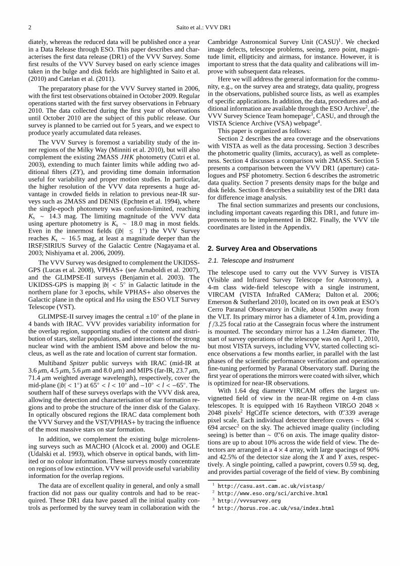
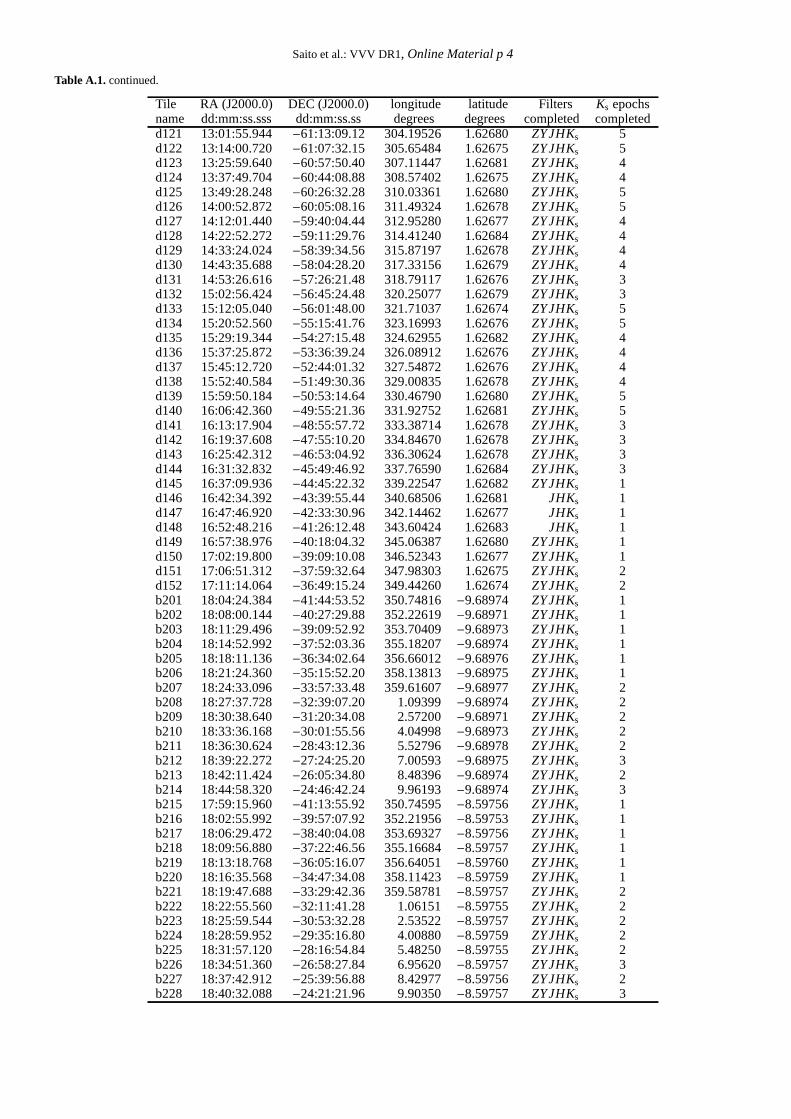
Here we list the tile centre coordinates for all VVV pointings.There are 196 bulge tiles, with names starting with ”b”, and 152tiles in the disk area, having names starting with ”d”. For eachtile we provide tile centre coordinates in Equatorial and Galacticcoordinates. All tiles have been observed using the identicaloffsetting strategy, combining 6 pawprints to contiguously fill1.5 × 1.1 sq. deg area. The second last column lists the filtersfor which the tile has been completed (i.e., observed withincon-straints), and the last column lists the number of epochs taken inKs band within the first observing season (DR1).

Saito et al.: VVV DR1, Online Material p 2
Table A.1. VVV Tile centres.
Tile RA (J2000.0) DEC (J2000.0) longitude latitude Filters Ks epochsname dd:mm:ss.sss dd:mm:ss.ss degrees degrees completed completedd001 11:43:24.936 −63:31:38.64 295.43770 −1.64975 ZYJHKs 5d002 11:56:12.576 −63:52:21.00 296.89672 −1.64979 ZYJHKs 5d003 12:09:17.184 −64:08:46.68 298.35572 −1.64971 ZYJHKs 5d004 12:22:35.184 −64:20:48.12 299.81470 −1.64971 ZYJHKs 5d005 12:36:02.640 −64:28:18.84 301.27373 −1.64973 ZYJHKs 5d006 12:49:35.184 −64:31:14.88 302.73271 −1.64977 ZYJHKs 5d007 13:03:08.352 −64:29:34.44 304.19170 −1.64978 ZYJHKs 5d008 13:16:37.632 −64:23:18.24 305.65072 −1.64970 ZYJHKs 5d009 13:29:58.632 −64:12:30.24 307.10972 −1.64971 JHKs 5d010 13:43:07.272 −63:57:15.84 308.56873 −1.64973 ZYJHKs 5d011 13:55:59.856 −63:37:42.60 310.02772 −1.64971 ZYJHKs 5d012 14:08:33.240 −63:14:00.24 311.48673 −1.64970 ZYJHKs 5d013 14:20:44.808 −62:46:19.92 312.94573 −1.64979 ZYJHKs 5d014 14:32:32.496 −62:14:52.80 314.40472 −1.64974 ZYJHKs 5d015 14:43:42.144 −61:40:33.96 315.83598 −1.64972 ZYJHKs 4d016 14:54:38.784 −61:02:16.44 317.29497 −1.64975 ZYJHKs 4d017 15:05:08.712 −60:20:51.00 318.75395 −1.64975 ZYJHKs 4d018 15:15:11.880 −59:36:30.60 320.21293 −1.64975 ZYJHKs 4d019 15:24:48.600 −58:49:27.84 321.67194 −1.64978 ZYJHKs 4d020 15:33:59.400 −57:59:54.60 323.13095 −1.64976 ZYJHKs 4d021 15:42:45.072 −57:08:02.40 324.58996 −1.64971 ZYJHKs 4d022 15:51:06.576 −56:14:02.40 326.04898 −1.64975 ZYJHKs 4d023 15:59:04.920 −55:18:04.32 327.50799 −1.64974 ZYJHKs 5d024 16:06:41.208 −54:20:17.88 328.96694 −1.64974 ZYJHKs 5d025 16:13:56.640 −53:20:51.36 330.42599 −1.64974 ZYJHKs 5d026 16:20:52.320 −52:19:53.40 331.88495 −1.64978 ZYJHKs 5d027 16:27:29.400 −51:17:30.84 333.34393 −1.64976 JHKs 2d028 16:33:49.032 −50:13:50.52 334.80299 −1.64976 JHKs 2d029 16:39:52.248 −49:08:58.92 336.26199 −1.64971 JHKs 2d030 16:45:40.128 −48:03:01.80 337.72099 −1.64973 ZYJHKs 2d031 16:51:13.632 −46:56:04.20 339.17999 −1.64971 ZYJHKs 2d032 16:56:33.720 −45:48:11.16 340.63896 −1.64975 ZYJHKs 2d033 17:01:41.256 −44:39:26.64 342.09795 −1.64972 ZYJHKs 1d034 17:06:37.104 −43:29:54.96 343.55695 −1.64975 ZYJHKs 1d035 17:11:22.032 −42:19:39.72 345.01595 −1.64979 ZYJHKs 1d036 17:15:56.760 −41:08:44.16 346.47495 −1.64979 JHKs 1d037 17:20:21.984 −39:57:11.16 347.93400 −1.64973 JHKs 1d038 17:24:38.352 −38:45:04.32 349.39294 −1.64975 JHKs 1d039 11:45:52.488 −62:28:17.40 295.43747 −0.55759 ZYJHKs 5d040 11:58:14.160 −62:48:15.12 296.89617 −0.55758 ZYJHKs 5d041 12:10:50.928 −63:04:04.80 298.35479 −0.55753 ZYJHKs 5d042 12:23:39.672 −63:15:39.60 299.81350 −0.55756 ZYJHKs 5d043 12:36:36.744 −63:22:53.40 301.27213 −0.55754 ZYJHKs 5d044 12:49:38.376 −63:25:42.96 302.73081 −0.55755 ZYJHKs 5d045 13:02:40.560 −63:24:06.84 304.18948 −0.55760 ZYJHKs 5d046 13:15:39.288 −63:18:05.40 305.64814 −0.55754 ZYJHKs 5d047 13:28:30.696 −63:07:42.24 307.10682 −0.55756 JHKs 5d048 13:41:11.112 −62:53:02.04 308.56549 −0.55756 JHKs 5d049 13:53:37.224 −62:34:12.00 310.02413 −0.55760 ZYJHKs 5d050 14:05:46.176 −62:11:20.04 311.48283 −0.55756 ZYJHKs 5d051 14:17:35.520 −61:44:36.60 312.94152 −0.55757 ZYJHKs 5d052 14:29:03.312 −61:14:12.48 314.40014 −0.55761 ZYJHKs 5d053 14:40:08.135 −60:40:18.48 315.85883 −0.55752 ZYJHKs 4d054 14:50:49.032 −60:03:07.56 317.31750 −0.55758 ZYJHKs 4d055 15:01:05.424 −59:22:51.24 318.77616 −0.55761 ZYJHKs 4d056 15:10:57.120 −58:39:41.40 320.23482 −0.55759 ZYJHKs 3d057 15:20:24.264 −57:53:49.92 321.69349 −0.55755 ZYJHKs 4d058 15:29:27.264 −57:05:28.32 323.15217 −0.55754 ZYJHKs 4d059 15:38:06.720 −56:14:47.40 324.61087 −0.55755 ZYJHKs 4d060 15:46:23.352 −55:21:57.60 326.06950 −0.55754 ZYJHKs 4

Saito et al.: VVV DR1, Online Material p 3
Table A.1. continued.
Tile RA (J2000.0) DEC (J2000.0) longitude latitude Filters Ks epochsname dd:mm:ss.sss dd:mm:ss.ss degrees degrees completed completedd061 15:54:18.096 −54:27:08.64 327.52817 −0.55761 ZYJHKs 5d062 16:01:51.840 −53:30:29.16 328.98684 −0.55756 ZYJHKs 5d063 16:09:05.616 −52:32:08.16 330.44549 −0.55755 ZYJHKs 5d064 16:16:00.456 −51:32:13.20 331.90419 −0.55754 ZYJHKs 5d065 16:22:37.368 −50:30:51.84 333.36286 −0.55756 JHKs 2d066 16:28:57.360 −49:28:10.56 334.82153 −0.55755 JHKs 2d067 16:35:01.416 −48:24:15.84 336.28015 −0.55756 JHKs 2d068 16:40:50.520 −47:19:13.08 337.73882 −0.55761 ZYJHKs 2d069 16:46:25.560 −46:13:07.32 339.19753 −0.55758 ZYJHKs 2d070 16:51:47.400 −45:06:03.96 340.65613 −0.55757 ZYJHKs 2d071 16:56:56.928 −43:58:06.96 342.11483 −0.55761 ZYJHKs 1d072 17:01:54.864 −42:49:20.28 343.57351 −0.55754 ZYJHKs 1d073 17:06:42.000 −41:39:48.24 345.03215 −0.55756 ZYJHKs 1d074 17:11:19.032 −40:29:33.72 346.49083 −0.55759 JHKs 1d075 17:15:46.608 −39:18:39.96 347.94953 −0.55759 JHKs 1d076 17:20:05.328 −38:07:09.84 349.40822 −0.55752 JHKs 1d077 11:48:10.080 −61:24:47.16 295.43749 0.53461 ZYJHKs 5d078 12:00:07.584 −61:44:03.84 296.89636 0.53458 ZYJHKs 5d079 12:12:18.648 −61:59:20.40 298.35521 0.53456 ZYJHKs 5d080 12:24:40.392 −62:10:30.00 299.81408 0.53461 ZYJHKs 5d081 12:37:09.600 −62:17:27.96 301.27295 0.53465 ZYJHKs 5d082 12:49:42.840 −62:20:11.40 302.73182 0.53458 ZYJHKs 5d083 13:02:16.560 −62:18:38.16 304.19066 0.53466 ZYJHKs 5d084 13:14:47.232 −62:12:50.04 305.64955 0.53458 ZYJHKs 5d085 13:27:11.328 −62:02:48.84 307.10837 0.53460 ZYJHKs 4d086 13:39:25.632 −61:48:39.24 308.56725 0.53465 ZYJHKs 4d087 13:51:27.144 −61:30:28.08 310.02613 0.53456 ZYJHKs 5d088 14:03:13.176 −61:08:22.20 311.48497 0.53458 ZYJHKs 5d089 14:14:41.544 −60:42:30.60 312.94386 0.53465 ZYJHKs 4d090 14:25:50.400 −60:13:03.72 314.40272 0.53463 ZYJHKs 4d091 14:36:38.352 −59:40:11.64 315.86159 0.53462 ZYJHKs 4d092 14:47:04.392 −59:04:05.52 317.32043 0.53461 ZYJHKs 4d093 14:57:07.920 −58:24:56.16 318.77932 0.53465 ZYJHKs 3d094 15:06:48.648 −57:42:55.44 320.23818 0.53459 ZYJHKs 3d095 15:16:06.552 −56:58:13.80 321.69700 0.53459 ZYJHKs 5d096 15:25:01.920 −56:11:02.04 323.15588 0.53461 ZYJHKs 5d097 15:33:35.208 −55:21:30.60 324.61479 0.53459 ZYJHKs 4d098 15:41:46.968 −54:29:49.20 326.07365 0.53465 ZYJHKs 4d099 15:49:37.968 −53:36:07.56 327.53250 0.53463 ZYJHKs 4d100 15:57:09.024 −52:40:34.32 328.99135 0.53458 ZYJHKs 4d101 16:04:20.976 −51:43:17.40 330.45023 0.53459 ZYJHKs 5d102 16:11:14.736 −50:44:24.72 331.90911 0.53460 ZYJHKs 5d103 16:17:51.216 −49:44:03.48 333.36798 0.53460 ZYJHKs 3d104 16:24:11.328 −48:42:20.16 334.82687 0.53461 ZYJHKs 3d105 16:30:15.960 −47:39:21.24 336.28568 0.53460 ZYJHKs 3d106 16:36:06.000 −46:35:12.12 337.74450 0.53460 ZYJHKs 3d107 16:41:42.312 −45:29:57.84 339.20338 0.53460 JHKs 1d108 16:47:05.712 −44:23:43.44 340.66229 0.53457 JHKs 1d109 16:52:16.944 −43:16:33.24 342.12118 0.53461 JHKs 1d110 16:57:16.776 −42:08:31.56 343.58005 0.53462 ZYJHKs 1d111 17:02:05.904 −40:59:42.36 345.03883 0.53459 ZYJHKs 1d112 17:06:45.024 −39:50:08.52 346.49771 0.53457 ZYJHKs 1d113 17:11:14.736 −38:39:53.28 347.95664 0.53461 ZYJHKs 2d114 17:15:35.640 −37:29:00.24 349.41546 0.53460 ZYJHKs 2d115 11:50:18.720 −60:21:09.00 295.43768 1.62680 ZYJHKs 5d116 12:01:53.760 −60:39:47.52 296.89732 1.62677 ZYJHKs 5d117 12:13:40.992 −60:54:32.75 298.35689 1.62684 ZYJHKs 5d118 12:25:37.800 −61:05:19.68 299.81648 1.62674 ZYJHKs 5d119 12:37:41.304 −61:12:02.52 301.27608 1.62684 ZYJHKs 5d120 12:49:48.408 −61:14:39.48 302.73567 1.62683 ZYJHKs 5
Saito et al.: VVV DR1, Online Material p 4
Table A.1. continued.
Tile RA (J2000.0) DEC (J2000.0) longitude latitude Filters Ks epochsname dd:mm:ss.sss dd:mm:ss.ss degrees degrees completed completedd121 13:01:55.944 −61:13:09.12 304.19526 1.62680 ZYJHKs 5d122 13:14:00.720 −61:07:32.15 305.65484 1.62675 ZYJHKs 5d123 13:25:59.640 −60:57:50.40 307.11447 1.62681 ZYJHKs 4d124 13:37:49.704 −60:44:08.88 308.57402 1.62675 ZYJHKs 4d125 13:49:28.248 −60:26:32.28 310.03361 1.62680 ZYJHKs 5d126 14:00:52.872 −60:05:08.16 311.49324 1.62678 ZYJHKs 5d127 14:12:01.440 −59:40:04.44 312.95280 1.62677 ZYJHKs 4d128 14:22:52.272 −59:11:29.76 314.41240 1.62684 ZYJHKs 4d129 14:33:24.024 −58:39:34.56 315.87197 1.62678 ZYJHKs 4d130 14:43:35.688 −58:04:28.20 317.33156 1.62679 ZYJHKs 4d131 14:53:26.616 −57:26:21.48 318.79117 1.62676 ZYJHKs 3d132 15:02:56.424 −56:45:24.48 320.25077 1.62679 ZYJHKs 3d133 15:12:05.040 −56:01:48.00 321.71037 1.62674 ZYJHKs 5d134 15:20:52.560 −55:15:41.76 323.16993 1.62676 ZYJHKs 5d135 15:29:19.344 −54:27:15.48 324.62955 1.62682 ZYJHKs 4d136 15:37:25.872 −53:36:39.24 326.08912 1.62676 ZYJHKs 4d137 15:45:12.720 −52:44:01.32 327.54872 1.62676 ZYJHKs 4d138 15:52:40.584 −51:49:30.36 329.00835 1.62678 ZYJHKs 4d139 15:59:50.184 −50:53:14.64 330.46790 1.62680 ZYJHKs 5d140 16:06:42.360 −49:55:21.36 331.92752 1.62681 ZYJHKs 5d141 16:13:17.904 −48:55:57.72 333.38714 1.62678 ZYJHKs 3d142 16:19:37.608 −47:55:10.20 334.84670 1.62678 ZYJHKs 3d143 16:25:42.312 −46:53:04.92 336.30624 1.62678 ZYJHKs 3d144 16:31:32.832 −45:49:46.92 337.76590 1.62684 ZYJHKs 3d145 16:37:09.936 −44:45:22.32 339.22547 1.62682 ZYJHKs 1d146 16:42:34.392 −43:39:55.44 340.68506 1.62681 JHKs 1d147 16:47:46.920 −42:33:30.96 342.14462 1.62677 JHKs 1d148 16:52:48.216 −41:26:12.48 343.60424 1.62683 JHKs 1d149 16:57:38.976 −40:18:04.32 345.06387 1.62680 ZYJHKs 1d150 17:02:19.800 −39:09:10.08 346.52343 1.62677 ZYJHKs 1d151 17:06:51.312 −37:59:32.64 347.98303 1.62675 ZYJHKs 2d152 17:11:14.064 −36:49:15.24 349.44260 1.62674 ZYJHKs 2b201 18:04:24.384 −41:44:53.52 350.74816 −9.68974 ZYJHKs 1b202 18:08:00.144 −40:27:29.88 352.22619 −9.68971 ZYJHKs 1b203 18:11:29.496 −39:09:52.92 353.70409 −9.68973 ZYJHKs 1b204 18:14:52.992 −37:52:03.36 355.18207 −9.68974 ZYJHKs 1b205 18:18:11.136 −36:34:02.64 356.66012 −9.68976 ZYJHKs 1b206 18:21:24.360 −35:15:52.20 358.13813 −9.68975 ZYJHKs 1b207 18:24:33.096 −33:57:33.48 359.61607 −9.68977 ZYJHKs 2b208 18:27:37.728 −32:39:07.20 1.09399 −9.68974 ZYJHKs 2b209 18:30:38.640 −31:20:34.08 2.57200 −9.68971 ZYJHKs 2b210 18:33:36.168 −30:01:55.56 4.04998 −9.68973 ZYJHKs 2b211 18:36:30.624 −28:43:12.36 5.52796 −9.68978 ZYJHKs 2b212 18:39:22.272 −27:24:25.20 7.00593 −9.68975 ZYJHKs 3b213 18:42:11.424 −26:05:34.80 8.48396 −9.68974 ZYJHKs 2b214 18:44:58.320 −24:46:42.24 9.96193 −9.68974 ZYJHKs 3b215 17:59:15.960 −41:13:55.92 350.74595 −8.59756 ZYJHKs 1b216 18:02:55.992 −39:57:07.92 352.21956 −8.59753 ZYJHKs 1b217 18:06:29.472 −38:40:04.08 353.69327 −8.59756 ZYJHKs 1b218 18:09:56.880 −37:22:46.56 355.16684 −8.59757 ZYJHKs 1b219 18:13:18.768 −36:05:16.07 356.64051 −8.59760 ZYJHKs 1b220 18:16:35.568 −34:47:34.08 358.11423 −8.59759 ZYJHKs 1b221 18:19:47.688 −33:29:42.36 359.58781 −8.59757 ZYJHKs 2b222 18:22:55.560 −32:11:41.28 1.06151 −8.59755 ZYJHKs 2b223 18:25:59.544 −30:53:32.28 2.53522 −8.59757 ZYJHKs 2b224 18:28:59.952 −29:35:16.80 4.00880 −8.59759 ZYJHKs 2b225 18:31:57.120 −28:16:54.84 5.48250 −8.59755 ZYJHKs 2b226 18:34:51.360 −26:58:27.84 6.95620 −8.59757 ZYJHKs 3b227 18:37:42.912 −25:39:56.88 8.42977 −8.59756 ZYJHKs 2b228 18:40:32.088 −24:21:21.96 9.90350 −8.59757 ZYJHKs 3
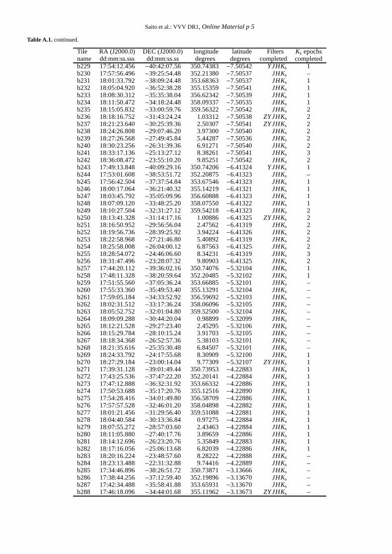
Saito et al.: VVV DR1, Online Material p 5
Table A.1. continued.
Tile RA (J2000.0) DEC (J2000.0) longitude latitude Filters Ks epochsname dd:mm:ss.sss dd:mm:ss.ss degrees degrees completed completedb229 17:54:12.456 −40:42:07.56 350.74383 −7.50542 YJHKs 1b230 17:57:56.496 −39:25:54.48 352.21380 −7.50537 JHKs –b231 18:01:33.792 −38:09:24.48 353.68363 −7.50537 JHKs 1b232 18:05:04.920 −36:52:38.28 355.15359 −7.50541 JHKs 1b233 18:08:30.312 −35:35:38.04 356.62342 −7.50539 JHKs 1b234 18:11:50.472 −34:18:24.48 358.09337 −7.50535 JHKs 1b235 18:15:05.832 −33:00:59.76 359.56322 −7.50542 JHKs 2b236 18:18:16.752 −31:43:24.24 1.03312 −7.50538 ZYJHKs 2b237 18:21:23.640 −30:25:39.36 2.50307 −7.50541 ZYJHKs 2b238 18:24:26.808 −29:07:46.20 3.97300 −7.50540 JHKs 2b239 18:27:26.568 −27:49:45.84 5.44287 −7.50536 JHKs 2b240 18:30:23.256 −26:31:39.36 6.91271 −7.50540 JHKs 2b241 18:33:17.136 −25:13:27.12 8.38261 −7.50541 JHKs 3b242 18:36:08.472 −23:55:10.20 9.85251 −7.50542 JHKs 2b243 17:49:13.848 −40:09:29.16 350.74206 −6.41324 YJHKs 1b244 17:53:01.608 −38:53:51.72 352.20875 −6.41323 JHKs –b245 17:56:42.504 −37:37:54.84 353.67546 −6.41323 JHKs 1b246 18:00:17.064 −36:21:40.32 355.14219 −6.41321 JHKs 1b247 18:03:45.792 −35:05:09.96 356.60888 −6.41323 JHKs 1b248 18:07:09.120 −33:48:25.20 358.07550 −6.41322 JHKs 1b249 18:10:27.504 −32:31:27.12 359.54218 −6.41323 JHKs 2b250 18:13:41.328 −31:14:17.16 1.00886 −6.41325 ZYJHKs 2b251 18:16:50.952 −29:56:56.04 2.47562 −6.41319 JHKs 2b252 18:19:56.736 −28:39:25.92 3.94224 −6.41326 JHKs 2b253 18:22:58.968 −27:21:46.80 5.40892 −6.41319 JHKs 2b254 18:25:58.008 −26:04:00.12 6.87563 −6.41325 JHKs 2b255 18:28:54.072 −24:46:06.60 8.34231 −6.41319 JHKs 3b256 18:31:47.496 −23:28:07.32 9.80903 −6.41325 JHKs 2b257 17:44:20.112 −39:36:02.16 350.74076 −5.32104 JHKs 1b258 17:48:11.328 −38:20:59.64 352.20485 −5.32102 JHKs 1b259 17:51:55.560 −37:05:36.24 353.66885 −5.32101 JHKs –b260 17:55:33.360 −35:49:53.40 355.13291 −5.32104 JHKs –b261 17:59:05.184 −34:33:52.92 356.59692 −5.32103 JHKs –b262 18:02:31.512 −33:17:36.24 358.06096 −5.32105 JHKs –b263 18:05:52.752 −32:01:04.80 359.52500 −5.32104 JHKs –b264 18:09:09.288 −30:44:20.04 0.98899 −5.32099 JHKs –b265 18:12:21.528 −29:27:23.40 2.45295 −5.32106 JHKs –b266 18:15:29.784 −28:10:15.24 3.91703 −5.32105 JHKs –b267 18:18:34.368 −26:52:57.36 5.38103 −5.32101 JHKs –b268 18:21:35.616 −25:35:30.48 6.84507 −5.32101 JHKs –b269 18:24:33.792 −24:17:55.68 8.30909 −5.32100 JHKs 1b270 18:27:29.184 −23:00:14.04 9.77309 −5.32107 ZYJHKs 1b271 17:39:31.128 −39:01:49.44 350.73953 −4.22883 JHKs 1b272 17:43:25.536 −37:47:22.20 352.20141 −4.22884 JHKs 1b273 17:47:12.888 −36:32:31.92 353.66332 −4.22886 JHKs 1b274 17:50:53.688 −35:17:20.76 355.12516 −4.22890 JHKs 1b275 17:54:28.416 −34:01:49.80 356.58709 −4.22886 JHKs 1b276 17:57:57.528 −32:46:01.20 358.04898 −4.22882 JHKs 1b277 18:01:21.456 −31:29:56.40 359.51088 −4.22881 JHKs 1b278 18:04:40.584 −30:13:36.84 0.97275 −4.22884 JHKs 1b279 18:07:55.272 −28:57:03.60 2.43463 −4.22884 JHKs 1b280 18:11:05.880 −27:40:17.76 3.89659 −4.22886 JHKs 1b281 18:14:12.696 −26:23:20.76 5.35849 −4.22883 JHKs 1b282 18:17:16.056 −25:06:13.68 6.82039 −4.22886 JHKs 1b283 18:20:16.224 −23:48:57.60 8.28222 −4.22888 JHKs –b284 18:23:13.488 −22:31:32.88 9.74416 −4.22889 JHKs –b285 17:34:46.896 −38:26:51.72 350.73871 −3.13666 JHKs –b286 17:38:44.256 −37:12:59.40 352.19896 −3.13670 JHKs –b287 17:42:34.488 −35:58:41.88 353.65931 −3.13670 JHKs –b288 17:46:18.096 −34:44:01.68 355.11962 −3.13673 ZYJHKs –

Saito et al.: VVV DR1, Online Material p 6
Table A.1. continued.
Tile RA (J2000.0) DEC (J2000.0) longitude latitude Filters Ks epochsname dd:mm:ss.sss dd:mm:ss.ss degrees degrees completed completedb289 17:49:55.536 −33:29:00.24 356.57994 −3.13668 ZYJHKs 1b290 17:53:27.288 −32:13:39.72 358.04023 −3.13673 ZYJHKs 1b291 17:56:53.736 −30:58:01.20 359.50054 −3.13672 ZYJHKs –b292 18:00:15.264 −29:42:06.12 0.96088 −3.13663 ZY –b293 18:03:32.280 −28:25:56.28 2.42120 −3.13666 ZY –b294 18:06:45.096 −27:09:32.75 3.88150 −3.13671 ZYJHKs –b295 18:09:54.024 −25:52:56.64 5.34179 −3.13672 ZYJHKs –b296 18:12:59.352 −24:36:09.00 6.80204 −3.13666 ZYJHKs –b297 18:16:01.416 −23:19:10.92 8.26235 −3.13668 ZYJHKs 1b298 18:19:00.456 −22:02:03.12 9.72271 −3.13666 JHKs 1b299 17:30:07.272 −37:51:11.88 350.73789 −2.04453 JHKs –b300 17:34:07.344 −36:37:53.76 352.19711 −2.04451 JHKs –b301 17:38:00.240 −35:24:09.00 353.65635 −2.04453 ZYJHKs –b302 17:41:46.440 −34:09:59.40 355.11565 −2.04449 ZYJHKs –b303 17:45:26.424 −32:55:27.48 356.57487 −2.04453 ZYJHKs 1b304 17:49:00.600 −31:40:34.32 358.03411 −2.04446 ZYJHKs 1b305 17:52:29.424 −30:25:22.08 359.49334 −2.04452 ZYJHKs –b306 17:55:53.256 −29:09:51.84 0.95261 −2.04456 ZYJHKs –b307 17:59:12.432 −27:54:05.04 2.41186 −2.04451 ZYJHKs –b308 18:02:27.312 −26:38:03.12 3.87111 −2.04447 ZYJHKs –b309 18:05:38.232 −25:21:47.52 5.33034 −2.04451 ZYJHKs –b310 18:08:45.480 −24:05:18.96 6.78962 −2.04454 ZYJHKs –b311 18:11:49.320 −22:48:38.52 8.24891 −2.04449 ZYJHKs 1b312 18:14:50.040 −21:31:47.64 9.70816 −2.04447 JHKs 1b313 17:25:32.232 −37:14:49.92 350.73753 −0.95236 JHKs 1b314 17:29:34.800 −36:02:05.64 352.19625 −0.95230 JHKs 1b315 17:33:30.168 −34:48:52.92 353.65504 −0.95232 JHKs 1b316 17:37:18.768 −33:35:14.28 355.11368 −0.95231 JHKs 1b317 17:41:01.104 −32:21:10.80 356.57248 −0.95229 JHKs 1b318 17:44:37.584 −31:06:45.00 358.03121 −0.95230 JHKs 1b319 17:48:08.616 −29:51:58.32 359.48996 −0.95233 JHKs 1b320 17:51:34.560 −28:36:52.56 0.94861 −0.95235 JHKs 1b321 17:54:55.800 −27:21:28.44 2.40742 −0.95234 JHKs 1b322 17:58:12.648 −26:05:48.12 3.86612 −0.95234 JHKs 1b323 18:01:25.416 −24:49:52.68 5.32477 −0.95232 JHKs 1b324 18:04:34.440 −23:33:42.84 6.78355 −0.95232 JHKs 1b325 18:07:39.984 −22:17:20.40 8.24226 −0.95238 JHKs –b326 18:10:42.288 −21:00:45.72 9.70101 −0.95231 JHKs –b327 17:21:01.656 −36:37:48.00 350.73744 0.13984 JHKs 1b328 17:25:06.528 −35:25:37.20 352.19621 0.13989 JHKs 1b329 17:29:04.152 −34:12:56.52 353.65492 0.13987 JHKs –b330 17:32:55.008 −32:59:47.76 355.11368 0.13984 JHKs –b331 17:36:39.504 −31:46:13.08 356.57236 0.13988 JHKs –b332 17:40:18.120 −30:32:14.28 358.03110 0.13982 JHKs –b333 17:43:51.192 −29:17:52.80 359.48985 0.13988 JHKs –b334 17:47:19.128 −28:03:10.80 0.94855 0.13988 JHKs –b335 17:50:42.288 −26:48:09.36 2.40731 0.13985 JHKs –b336 17:54:00.984 −25:32:49.92 3.86610 0.13985 JHKs –b337 17:57:15.528 −24:17:14.28 5.32478 0.13981 JHKs –b338 18:00:26.208 −23:01:23.16 6.78348 0.13983 JHKs –b339 18:03:33.336 −21:45:17.64 8.24226 0.13983 JHKs 1b340 18:06:37.152 −20:28:59.16 9.70099 0.13985 ZYJHKs 1b341 17:16:35.472 −36:00:07.56 350.73765 1.23203 ZYJHKs 1b342 17:20:42.432 −34:48:30.24 352.19686 1.23205 JHKs 1b343 17:24:42.144 −33:36:20.88 353.65613 1.23203 JHKs 1b344 17:28:35.040 −32:23:41.64 355.11542 1.23207 JHKs 1b345 17:32:21.576 −31:10:35.04 356.57468 1.23205 JHKs 1b346 17:36:02.160 −29:57:02.52 358.03399 1.23203 JHKs 1b347 17:39:37.152 −28:43:06.24 359.49322 1.23206 JHKs 1b348 17:43:06.960 −27:28:47.64 0.95251 1.23203 JHKs 1

Saito et al.: VVV DR1, Online Material p 7
Table A.1. continued.
Tile RA (J2000.0) DEC (J2000.0) longitude latitude Filters Ks epochsname dd:mm:ss.sss dd:mm:ss.ss degrees degrees completed completedb349 17:46:31.896 −26:14:08.52 2.41172 1.23201 JHKs 1b350 17:49:52.296 −24:59:09.96 3.87096 1.23204 JHKs 1b351 17:53:08.496 −23:43:53.40 5.33027 1.23202 JHKs –b352 17:56:20.760 −22:28:20.28 6.78955 1.23201 ZYJHKs –b353 17:59:29.376 −21:12:31.68 8.24885 1.23202 ZYJHKs –b354 18:02:34.608 −19:56:29.04 9.70808 1.23199 ZYJHKs –b355 17:12:13.584 −35:21:49.68 350.73827 2.32427 ZYJHKs 1b356 17:16:22.488 −34:10:45.12 352.19857 2.32417 ZY 1b357 17:20:24.096 −32:59:06.36 353.65894 2.32423 ZY –b358 17:24:18.888 −31:46:56.64 355.11924 2.32422 ZY –b361 17:35:26.472 −28:07:39.36 359.50024 2.32421 ZY –b362 17:38:58.008 −26:53:43.80 0.96059 2.32418 ZYJHKs –b363 17:42:24.624 −25:39:25.92 2.42098 2.32420 ZYJHKs –b364 17:45:46.632 −24:24:47.88 3.88124 2.32419 ZYJHKs –b365 17:49:04.368 −23:09:50.40 5.34158 2.32416 ZYJHKs –b366 17:52:18.096 −21:54:34.92 6.80192 2.32418 JHKs 1b367 17:55:28.104 −20:39:02.88 8.26224 2.32419 JHKs 1b368 17:58:34.656 −19:23:15.00 9.72265 2.32423 JHKs 1b369 17:07:55.872 −34:42:57.24 350.73892 3.41637 ZYJHKs 1b370 17:12:06.480 −33:32:24.36 352.20083 3.41644 ZYJHKs 1b371 17:16:09.864 −32:21:16.20 353.66280 3.41638 ZYJHKs –b372 17:20:06.384 −31:09:35.28 355.12466 3.41637 ZYJHKs –b373 17:23:56.496 −29:57:23.04 356.58663 3.41642 ZYJHKs –b374 17:27:40.584 −28:44:42.36 358.04853 3.41640 ZYJHKs –b375 17:31:19.032 −27:31:34.68 359.51046 3.41635 ZYJHKs –b376 17:34:52.152 −26:18:01.44 0.97243 3.41644 ZYJHKs –b377 17:38:20.328 −25:04:05.16 2.43434 3.41638 ZYJHKs –b378 17:41:43.848 −23:49:46.56 3.89631 3.41638 ZYJHKs –b379 17:45:03.024 −22:35:07.44 5.35828 3.41637 ZYJHKs 1b380 17:48:18.120 −21:20:09.24 6.82020 3.41640 ZYJHKs 1b381 17:51:29.424 −20:04:53.40 8.28204 3.41640 JHKs 1b382 17:54:37.224 −18:49:20.64 9.74399 3.41636 JHKs 1b383 17:03:42.216 −34:03:30.60 350.73979 4.50856 ZYJHKs 1b384 17:07:54.408 −32:53:29.40 352.20380 4.50857 JHKs 1b385 17:11:59.352 −31:42:51.12 353.66783 4.50858 JHKs 1b386 17:15:57.480 −30:31:37.92 355.13195 4.50860 JHKs 1b387 17:19:49.176 −29:19:52.68 356.59597 4.50856 JHKs 1b388 17:23:34.824 −28:07:36.84 358.06004 4.50857 JHKs 1b389 17:27:14.784 −26:54:52.56 359.52411 4.50859 JHKs 1b390 17:30:45.384 −25:43:05.52 0.96034 4.50854 JHKs 1b391 17:34:15.096 −24:29:30.12 2.42444 4.50852 JHKs 1b392 17:37:40.080 −23:15:31.32 3.88850 4.50858 JHKs 1b393 17:41:00.672 −22:01:10.92 5.35253 4.50853 JHKs –b394 17:44:17.136 −20:46:29.64 6.81666 4.50854 JHKs –b395 17:47:29.736 −19:31:29.28 8.28074 4.50857 ZYJHKs –b396 17:50:38.736 −18:16:11.28 9.74476 4.50855 ZYJHKs –