W AS THERE MONETARY AUTONOMY IN EUROPE ON · PDF fileW AS THERE MONETARY AUTONOMY IN EUROPE ON ... the loss of monetary autonomy in Europe ... began to circulate and replaced the old

185WAS THERE MONETARY AUTONOMY IN EUROPE ON THE EVE OF EMU?Journal of Applied Economics, Vol. V, No. 2 (Nov 2002), 185-207

WAS THERE MONETARY AUTONOMY IN EUROPEON THE EVE OF EMU? THE GERMAN DOMINANCE

HYPOTHESIS RE-EXAMINED

OSCAR BAJO-RUBIO *

Universidad de Castilla-La Mancha

and

M. DOLORES MONTÁVEZ -GARCÉS*

Universidad Pública de Navarra

In this paper we re-examine the German dominance hypothesis, as a way to assess whetherthe loss of monetary autonomy in Europe associated with EMU had been significant. Weuse Granger-causality tests between the interest rates of Germany and all the countriesparticipating in the European Monetary System, with the sample period running untilDecember 1998. Our results would support a weak version of the hypothesis, with Germanyplaying a certain “leadership” or special role in the EMS, although she would not had been

strictly the “dominant” player.

JEL classification codes: F33, F36, E50

Key words: European monetary union, German dominance hypothesis,

Granger-causality

I. Intr oduction

Beginning on January 1st 1999, when a common currency, the euro, was

adopted, and the European Central Bank started its operations, 12 European

countries formed a monetary union (the Economic and Monetary Union,

* We are very grateful to Vicente Esteve, Simón Sosvilla-Rivero, and the co-editor of theJournal, Jorge Streb, for helpful comments and advice on a previous version. The usualdisclaimer applies.

186 JOURNAL OF APPLIED ECONOMICS

EMU). More recently, EMU can be said to be fully in force, once the euro

began to circulate and replaced the old national currencies after January 1st

2002.

As it becomes obvious, EMU means the loss of monetary independence

of the participating countries, which might be seen as a cost, at least at first

sight. Things are not so simple, however. It is well known that, according to

the so-called “inconsistent trinity” principle, a fixed exchange rate, full capital

mobility, and the independence of monetary policy are not mutually

compatible. And this situation roughly applied to the European economies

before EMU, which shared a quasi-fixed exchange rate system (the European

Monetary System, EMS), especially so following the elimination of capital

controls after the Single European Act in 1990-92. This fact led to the countries

participating in the EMS to realize that they were gradually losing the control

of their monetary policies in favor of the Bundesbank, the central bank of

Germany, i.e., the country presumed to act as a leader in the EMS. Hence,

EMU could emerge as an economic response to that situation, allowing those

countries to regain some control over monetary policy thanks to the creation

of an European Central Bank, in which they could have a vote (Wyplosz,

1997).

The possible dominant role of Germany within the EMS, prior to the start

of EMU, will be the subject of this paper. This could be of interest in order to

assess whether the loss of monetary autonomy in Europe associated with

EMU has been significant; which, in turn, could be taken as an argument in

favor of EMU itself. The empirical methodology makes use of Granger-

causality tests between the monthly interest rates of Germany and all the

countries participating at any time in the exchange rate mechanism (ERM) of

the EMS, with the sample period running until December 1998.

The rest of the paper is structured as follows. A brief review of the previous

literature on the subject, together with the contributions of the paper, is

provided in Section II. The econometric methodology and empirical results

are discussed in Section III. Finally, the main conclusions are presented in

Section IV.

187WAS THERE MONETARY AUTONOMY IN EUROPE ON THE EVE OF EMU?

II. Review of the Literature

In general terms, prior to EMU a broad consensus emerged in Europe

which would justify the argument that the EMS had worked in an asymmetric

way, with Germany assuming the leading role and the remaining countries

passively adjusting to German monetary policy actions. In turn, these countries

would have benefited from behaving in such a way, since they would have

taken advantage of the firmly established anti-inflation credibility of the

Bundesbank (see, e.g., Giavazzi and Pagano, 1988; or Mélitz, 1988). This

discussion ultimately lies in the so-called n - 1 problem faced by fixed exchange

rate systems, since there are only n - 1 exchange rates among the n countries

participating in an exchange rate agreement. Therefore, in such a situation,

either one country becomes the leader and sets monetary policy independently

(with the other countries following it), or all countries are allowed to decide

jointly over the implementation of monetary policy (De Grauwe, 2000).

The first empirical studies on the subject seemed to confirm the hypothesis

of German dominance into the EMS (see, e.g., Giavazzi and Giovannini,

1987, 1989, or Karfakis and Moschos, 1990). However, these conclusions

were not confirmed in further research, most of it consisting of tests for

Granger-causality between German and other countries’ interest rates at a

monthly or quarterly frequency (see, among others, Cohen and Wyplosz, 1989;

von Hagen and Fratianni, 1990; Koedijk and Kool, 1992; Katsimbris and

Miller, 1993; or Hassapis, Pittis and Prodromidis, 1999). In this way, a milder

support for the hypothesis was found in the above quoted papers; namely,

that the other countries’ interest rates depended on the German ones, but also

conversely, even though in a lower extent in terms of both size and persistence.

Finally, some results along these lines were also reported in other studies

using high frequency (i.e., daily) data on interest rates (see Gardner and

Perraudin, 1993; Henry and Weidmann, 1995; and Bajo, Sosvilla and

Fernández, 2001), so that it might seem that Germany would have played a

special role in the EMS, although calling it “dominance” would be too strong.

As stated in the Introduction, in this paper we re-examine the German


dominance hypothesis, as a way to assess whether the loss of monetary

autonomy in Europe associated with EMU has been significant. The paper

contributes to the existing literature in the following respects:

a. The sample period covers until just the eve of EMU, i.e., December 1998.

This allows us to include the most recent events in European monetary

history, such as the German reunification, the monetary turmoil at the end

of 1992, the broadening of the EMS fluctuation bands in August 1993,

and the rather quiet period leading to the birth of EMU. Regarding previous

studies on the subject, those with a more recent sample period are Hassapis,

Pittis and Prodromidis (1999), who use quarterly data until the end of

1994, and Bajo, Sosvilla and Fernández (2001), who use daily data until

February 1997.

b. The analysis is extended to all the countries participating at any time in

the ERM of the EMS. So, unlike previous studies (with the only exception

of Bajo, Sosvilla and Fernández, 2001), that consider only the founding

members of the EMS (i.e., Germany, France, Italy, Belgium, the

Netherlands, Denmark, and Ireland), our analysis also includes those

countries which later joined the ERM of the EMS (i.e., Spain, the UK,

and Portugal).

c. Granger-causality in a cointegration setting is properly tested. That is, an

error-correction mechanism (ECM) is included into every equation to be

estimated when cointegration is found, which allows us to distinguish

between short-run and long-run Granger-causality.1 Also, and following

Katsimbris and Miller’s (1993) suggestion, Granger-causality relationships

between German and the other countries’ interest rates have been

investigated both in a bivariate and a trivariate setting, in order to avoid

possible spurious results due to the omission of some relevant variable. As

usual, the US interest rates is the additional variable added to the analysis.

1 Katsimbris and Miller (1993) were the first to notice this point, usually overlooked in theavailable empirical studies on this subject.


d. Finally, and given the importance of the choice of lag lengths in Granger-

causality tests, these have been selected by means of an appropriate method.

In particular, we have used Hsiao’s (1981) sequential approach, specifically

designed to avoid imposing often false or spurious restrictions on the model.

Notice that, unlike the VAR approach performed in other studies (i.e.,

Hassapis, Pittis and Prodromidis, 1999), our procedure implies that, for

any pair of variables tested for Granger-causality between them, the number

of lags of the right-hand side variables is not constrained to be the same.

III. Econometric Methodology and Empirical Results

The econometric methodology used in this paper is based on Granger-

causality tests (Granger, 1969). As is well known, the results from these tests

are highly sensitive to the order of lags in the autoregressive process. In this

paper, we will identify the order of lags for each variable by means of Hsiao’s

(1981) sequential approach, which is based on Granger’s concept of causality

and Akaike’s final prediction error criterion.

Suppose we have two stationary variables, Xt and Y

t, which we would like

to test for Granger-causality. Consider the models:

The following steps are then used to apply Hsiao’s procedure:

i. Take Xt to be a univariate autoregressive process as in (1), and compute its

final prediction error (FPE hereafter) with the order of lags i varying from

1 to M. Choose the lag that yields the smallest FPE, say m, and denote the

corresponding FPE as FPEX

(m, 0).

ii. Treat Xt as a controlled variable with m lags, add lags of Y

t to (1) as in (2),

∑ ++==

−m

ititit uXX

1βα (1)

∑ +∑++== =

−−m

it

n

jjtjitit vYXX

1 1γβα (2)


and compute the FPEs with the order of lags j varying from 1 to N. Choose

the lag that yields the smallest FPE, say n, and denote the corresponding

FPE as FPEX

(m, n).

iii. Compare FPEX (m, 0) with FPE

X (m, n). If FPE

X (m, 0) > FPE

X (m, n), then

Yt is said to Granger-cause X

t, whereas if FPE

X (m, 0) < FPE

X (m, n), then

Xt would not be Granger-caused by Y

t.

Finally, steps (i) - (iii) should be repeated with Yt as the dependent variable

in order to test whether or not Xt Granger-causes Y

t.

Recall the earlier assumption that Xt and Y

t were stationary variables.

However, if they are integrated of order one (i.e., first-difference stationary),

I(1), and are cointegrated, (1) and (2) need to be amended to:

where zt is the ECM (Engle and Granger, 1987). Notice that if X

t and Y

t are

I(1) but are not cointegrated, the coefficient δ in (3) and (4) would be equal to

zero.

Now, the previous definitions of Granger-causality for stationary variables

can be applied to the case of I(1) variables from (3) and (4). In particular, if

FPE∆X (m, 0) > FPE∆X

(m, n), Yt is said to Granger-cause X

t in the short run;

and if δ is significantly different from zero, Yt is said to Granger-cause X

t in

the long run. Conversely, if FPE∆X (m, 0) < FPE∆X

(m, n), Xt would not be

Granger-caused by Yt in the short run; and if δ is not significantly different

from zero, Xt would not be Granger-caused by Y

t in the long run. As before,

the procedure should be repeated with ∆Yt as the dependent variable so that

the hypothesis of short-run and long-run Granger-causality from Xt to Y

t can

be tested.

∑ ++∆+=∆=

−−m

ittitit uzXX

11δβα (3)

∑ ++∑ ∆+∆+=∆=

−=

−−m

itt

n

jjtjitit vzYXX

11

1δγβα (4)


The data used in this paper are the three-month interbank onshore interest

rates, at a monthly frequency, of Germany, France, Italy, Belgium, the

Netherlands, Denmark, Ireland, Spain, the UK, Portugal, and the US. The

previous list includes all the European countries participating at any time in

the ERM of the EMS, and coincides with that of the countries joining EMU

from the outset, with the exceptions of Denmark and the UK, and the inclusion

of Luxembourg, Austria and Finland.2 The beginning of the sample period is

March 1979 (i.e., when the ERM started to operate) for the founding members

of the EMS (France, Italy, Belgium, the Netherlands, Denmark, and Ireland),

and the month of accession to the ERM for the newcomers: June 1989 for

Spain, October 1990 for the UK, and April 1992 for Portugal, with the data

for Germany and the US adjusting accordingly in each case. The end of the

sample is in all cases December 1998 (i.e., the last month before the starting

of EMU), and all the data come from the Boletín Estadístico (Statistical

Bulletin) of the Bank of Spain.

As a first step of the analysis, we tested for the order of integration of the

variables by means of two alternative tests. On the one hand, the Phillips-

Perron test (Phillips and Perron, 1988), which corrects, in a non-parametric

way, the possible presence of autocorrelation in the standard Dickey-Fuller

test, under the null hypothesis that the variable has a unit root. And, on the

other hand, given the small power of this test under certain stochastic properties

of the series, the KPSS test (Kwiatkowski, Phillips, Schmidt and Shin, 1992),

for which the null hypothesis is that of stationarity, unlike the standard Dickey-

Fuller-type tests. According to the results shown in parts A and B of Table 1,

for the Phillips-Perron test the null hypothesis of a unit root was not rejected

in all cases, at the same time that the null of a second unit root was always

rejected; in turn, for the KPSS test, the null hypothesis of stationarity was

always rejected.

2 Notice that Luxembourg, a founding member of the EMS, is not included in the samplesince she already formed a monetary union with Belgium before EMU. Also, Austria andFinland, who participated in the ERM of the EMS since January 1995 and October 1996,respectively, are not included given the small number of observations available.


Next, we tested for cointegration between the German interest rate and the

interest rates of the other European countries in our sample, both in a bivariate

and trivariate setting, in the latter case including the US interest rate as an

additional variable. To this end, we made use of Shin’s (1994) approach, which

is based on the application of the KPSS test on the residuals from the (bivariate

or trivariate) cointegrating regressions estimated by the method proposed by

Stock and Watson (1993). This method consists of estimating a dynamic long-

run regression that includes leads and lags of the first differences of the

explanatory variables, and provides a robust correction to the possible presence

of endogeneity among these variables, as well as of serial correlation of the

estimated errors.

Table 1.A. Unit Root Tests. Phillips-Perron Test

Levels First Differences

Z(tα~ ) Z(tα*) Z( α̂t ) Z(tα~ ) Z(tα*) Z( α̂t )

Germany -2.07 -1.26 -0.59 -11.29a -11.23a -11.23a

Belgium -3.52c -1.09 -0.81 -12.78a -12.72a -12.71a

Denmark -2.68 -1.05 -1.19 -10.52a -10.51a -10.48a

Spain -2.47 -0.05 -2.15b -8.87a -8.86a -8.32a

France -3.59b -1.03 -0.73 -11.39a -11.29a -11.28a

Netherlands -2.09 -1.29 -0.95 -12.88a -12.86a -12.85a

Ireland -3.13 -1.61 -1.21 -12.40a -12.39a -12.36a

Italy -3.19 -0.39 -0.82 -12.39a -12.22a -12.19a

Portugal -3.12 -1.07 -2.61a -7.71a -7.69a -7.28a

UK -2.18 -3.24b -2.75a -5.47a -5.27a -5.05a

US -3.23 -1.85 -1.12 -10.86a -10.86a -10.85a

Notes: Z( α~t ), Z(tα*) and Z( α̂t ) are the Phillips-Perron statistics with drift and trend, withdrift, and without drift, respectively. (a), (b), and (c) denote significance at the 1%, 5%,and 10% levels, respectively. The critical values are taken from MacKinnon (1991).

Country


Table 1.B. Unit Root Tests. KPSS Test

Levels

ηµ ητ

Germany 0.42c 0.14c

Belgium 1.27a 0.11

Denmark 1.26a 0.14c

Spain 0.94a 0.05

France 1.20a 0.11

Netherlands 0.68b 0.15b

Ireland 1.42a 0.08

Italy 1.27a 0.08

Portugal 0.77a 0.09

UK 0.48b 0.22a

US 1.23a 0.17b

Notes: ηµ, and ητ are the KPSS statistics with trend, and without trend, respectively. (a),(b), and (c) denote significance at the 1%, 5%, and 10% levels, respectively. The criticalvalues are taken from Kwiatkowski et al. (1992).

Country

The results of the cointegration test appear in Table 2. Recall that the null

hypothesis in the Shin test is that of cointegration instead of no cointegration,

unlike other more standard tests. As can be seen, the only interest rates

appearing to be cointegrated with the German ones, both in the bivariate and

the trivariate case (i.e., when the US interest rates are included into the

cointegration equation), would be those of Spain and the UK; even though in

the case of Portugal cointegration would be rejected just at a 10% significance

level. Notice that the data for these three countries cover a remarkably shorter

period as compared to the founding members of the EMS. In this sense, as

Caporale and Pittis (1995) observe, the integration of the financial markets of

the EMS countries would have been a gradual process, leading to a slow


convergence process of interest rates towards the German levels.3 Hence, as

long as a greater convergence should have been achieved for the last years of

the sample period, this might help to explain the finding of cointegration just

in the case of the newcomers to the EMS.

3 Some evidence along these lines for the Spanish case can be found in Camarero, Esteveand Tamarit (1997).

Table 2. Shin Cointegration Test

Country Bivariate Trivariate

Belgium 1.25a 0.53a

Denmark 1.13a 0.38b

Spain 0.18 0.10

France 1.14a 0.49a

Netherlands 0.76a 0.29b

Ireland 1.18a 0.45a

Italy 1.12a 0.43a

Portugal 0.26c 0.20c

UK 0.10 0.12

Notes: The test refers to the Cµ statistic on the DOLS residuals. (a), (b), and (c) denotesignificance at the 1%, 5%, and 10% levels, respectively. The critical values are taken fromShin (1994).

Now, we are able to perform Granger-causality tests in a cointegration

framework, and the results for the bivariate case are shown in Table 3. German

interest rates appear to Granger-cause all the other EMS interest rates, the

opposite being also true in all cases but that of Ireland. Notice, however, that,

when bilateral Granger-causality is found, the decrease in FPEs is greater

when German interest rates are added to the equations explaining the other

interest rates than in the opposite case. On the other hand, German interest

rates would cause those of Spain and the UK in the long run, but not the other


way round. These results would suggest that, despite the presence of some

degree of symmetry in the EMS, the influence of Germany on the other EMS

countries would have been greater than the other way round.

Table 3. Granger-Causality Tests: Bivariate Models

FPE FPE ECM Causality FPE FPE ECM Causality

{m, 0} {m, n} X → G {m, 0} {m, n} G → X

Belgium 0.099 0.096 --- YES 0.349 0.312 --- YES

{12, 0} {12, 12} {5, 0} {5, 5}

Denmark 0.099 0.098 --- YES 0.358 0.338 --- YES

{12, 0} {12, 8} {4, 0} {4, 5}

Spain 0.031 0.027 -0.005 YES 0.134 0.105 -0.043b YES

{4, 0} {4, 4} (-0.519) {4, 0} {4, 7} (-2.203)

France 0.099 0.094 --- YES 0.261 0.204 --- YES

{12, 0} {12, 10} {6, 0} {6, 6}

Netherlands 0.099 0.096 --- YES 0.097 0.091 --- YES

{12, 0} {12, 10} {12, 0} {12, 5}

Ireland 0.099 0.100 --- NO 0.627 0.615 --- YES

{12, 0} {12, 1} {6, 0} {6, 1}

Italy 0.099 0.099 --- YES 0.309 0.300 --- YES

{12, 0} {12, 10} {11, 0} {11, 4}

Portugal 0.030 0.029 --- YES 0.427 0.403 --- YES

{1, 0} {1, 2} {5, 0} {5, 4}

UK 0.029 0.028 -0.030 YES 0.063 0.051 -0.076a YES

{4, 0} {4, 2} (-1.594) {4, 0} {4, 5} (-2.785)

Notes: m and n denote the lags for the dependent variable and the additional regressor,respectively, leading to the smallest FPE in each case; the maximum number of lags triedhas been 12. X and G denote every country in the first column of the table, and Germany,respectively. (a), (b), and (c) denote significance at the 1%, 5%, and 10% levels, respectively,for the t-statistics of the ECMs (in parentheses).

Country


Next, we turn to the trivariate case in Table 4. Beginning with causality

between German interest rates and those of the other EMS countries, the

results, shown in part A of Table 4, are quite similar to those in Table 3. The

only exception would be that bilateral Granger-causality is now found for

Ireland too; also, the German interest rates do not appear to Granger-cause

the Spanish ones in the long run. Again, the German interest rates add more

explanatory power to the equations explaining the other interest rates than in

the opposite case.

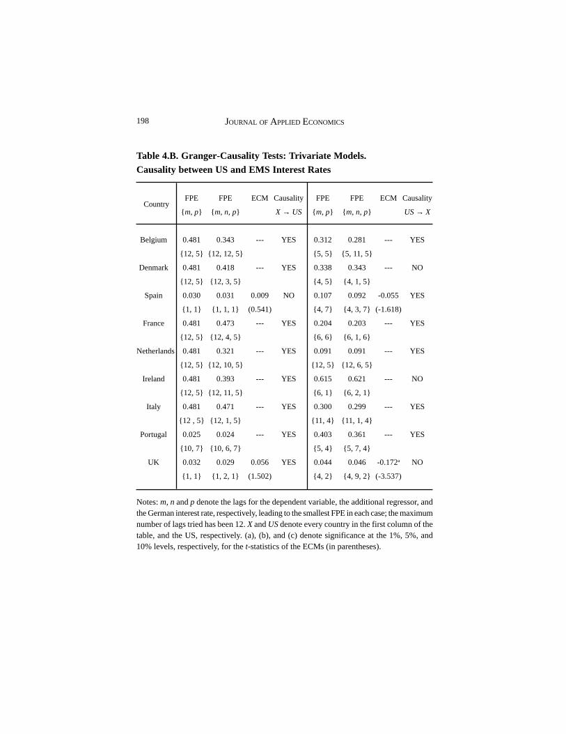
In order to get a more complete picture, we have also tested for Granger-

causality between the US interest rates and those of the EMS countries other

than Germany, as well as between German and US interest rates, with the

results appearing in parts B and C of Table 4, respectively. As can be seen,

the US interest rates would Granger-cause all the other interest rates, other

than those of Denmark, Ireland, and the UK; however, long-run Granger-

causality would appear in the UK case. In turn, the interest rates of all the

EMS countries, with the only exception of Spain, would Granger-cause the

US interest rates in the short run. On the other hand, bilateral short-run

Granger-causality is found between German and US interest rates in most

cases; the exceptions would be when the interest rates of Spain, the UK and

Portugal are included in the regressions, since Granger-causality only appears

from German to US rates in the first two cases, and no Granger-causality is

detected in the latter.

Overall, the results in parts B and C of Table 4 shed some additional light,

and complement those previously obtained in part A of the same table.

Although strongly influenced by the German ones, the interest rates of the

EMS countries would appear involved in a more complex web of

interdependences, as a result of the high degree of capital mobility existing

across the world economy. In particular, they would appear to be mutually

connected to the US interest rates, both directly and indirectly through the

German ones.

Finally, we have also tested for structural change in all the estimated

equations shown in Tables 3 and 4, by means of the Chow test. The dates


Table 4.A. Granger-Causality Tests: Trivariate Models.Causality between German and EMS Interest Rates


[m, p} [m, n, p} X → G [m, p} [m, n, p} G → X

Belgium 0.089 0.086 --- YES 0.255 0.229 --- YES

{12, 10} {12, 1, 10} {10, 12} {10, 4, 12}

Denmark 0.089 0.086 --- YES 0.352 0.340 --- YES

{12, 10} {12, 1, 10} {4, 8} {4, 5, 8}

Spain 0.030 0.029 0.022 YES 0.131 0.116 -0.052 YES

{4, 1} {4, 2, 1} (1.327) {4, 1} {4, 7, 1} (-1.465)

France 0.089 0.081 --- YES 0.247 0.211 --- YES

{12, 10} {12, 10, 10} {6, 12} {6, 6, 12}


{12, 10} {12, 1, 10} {12, 7} {12, 5, 7}

Ireland 0.089 0.086 --- YES 0.632 0.621 --- YES

{12, 12} {12, 1, 12} {6, 2} {6, 1, 2}

Italy 0.089 0.088 --- YES 0.311 0.299 --- YES

{12, 10} {12, 9, 10} {12, 1} {12, 4, 1}

Portugal 0.031 0.030 --- YES 0.394 0.345 --- YES

{1, 1} {1, 2, 1} {5, 7} {5, 12, 7}

UK 0.031 0.030 -0.028 YES 0.050 0.048 -0.191a YES

{4, 1} {4, 3, 1} (-0.621) {4, 1} {4, 5, 1} (-3.708)

Notes: m, n and p denote the lags for the dependent variable, the additional regressor, andthe US interest rate, respectively, leading to the smallest FPE in each case; the maximumnumber of lags tried has been 12. X and G denote every country in the first column of thetable, and Germany, respectively. (a), (b), and (c) denote significance at the 1%, 5%, and10% levels, respectively, for the t-statistics of the ECMs (in parentheses).

Country


Table 4.B. Granger-Causality Tests: Trivariate Models.Causality between US and EMS Interest Rates


{m, p} {m, n, p} X → US {m, p} {m, n, p} US → X

Belgium 0.481 0.343 --- YES 0.312 0.281 --- YES

{12, 5} {12, 12, 5} {5, 5} {5, 11, 5}

Denmark 0.481 0.418 --- YES 0.338 0.343 --- NO

{12, 5} {12, 3, 5} {4, 5} {4, 1, 5}

Spain 0.030 0.031 0.009 NO 0.107 0.092 -0.055 YES

{1, 1} {1, 1, 1} (0.541) {4, 7} {4, 3, 7} (-1.618)

France 0.481 0.473 --- YES 0.204 0.203 --- YES

{12, 5} {12, 4, 5} {6, 6} {6, 1, 6}


{12, 5} {12, 10, 5} {12, 5} {12, 6, 5}

Ireland 0.481 0.393 --- YES 0.615 0.621 --- NO

{12, 5} {12, 11, 5} {6, 1} {6, 2, 1}

Italy 0.481 0.471 --- YES 0.300 0.299 --- YES

{12 , 5} {12, 1, 5} {11, 4} {11, 1, 4}

Portugal 0.025 0.024 --- YES 0.403 0.361 --- YES

{10, 7} {10, 6, 7} {5, 4} {5, 7, 4}

UK 0.032 0.029 0.056 YES 0.044 0.046 -0.172a NO

{1, 1} {1, 2, 1} (1.502) {4, 2} {4, 9, 2} (-3.537)

Notes: m, n and p denote the lags for the dependent variable, the additional regressor, andthe German interest rate, respectively, leading to the smallest FPE in each case; the maximumnumber of lags tried has been 12. X and US denote every country in the first column of thetable, and the US, respectively. (a), (b), and (c) denote significance at the 1%, 5%, and10% levels, respectively, for the t-statistics of the ECMs (in parentheses).

Country


Table 4.C. Granger-Causality Tests: Trivariate Models.Causality between US and German Interest Rates


{m, p} {m, n, p} G → US {m, p} {m, n, p} US → G

Belgium 0.475 0.407 --- YES 0.096 0.086 --- YES

{12, 12}{12, 12, 12} {12, 12}{12, 10, 12}

Denmark 0.428 0.418 --- YES 0.098 0.090 --- YES

{12, 3} {12, 5, 3} {12, 8} {12, 10, 8}

Spain 0.032 0.031 0.009 YES 0.029 0.029 0.016 NO

{1, 1} {1, 1, 1} (0.541) {4, 2} {4, 1, 2} (0.975)

France 0.487 0.484 --- YES 0.094 0.079 --- YES

{12, 1} {12, 5, 1} {12, 10}{12, 12, 10}


{12, 5} {12, 10, 5} {12, 10}{12, 12, 10}

Ireland 0.402 0.389 --- YES 0.100 0.090 --- YES

{12, 11} {12, 2, 11} {12, 1} {12, 10, 1}

Italy 0.474 0.471 --- YES 0.097 0.089 --- YES

{12, 1} {11, 4, 1} {12, 10}{12, 10, 10}

Portugal 0.024 0.024 --- NO 0.029 0.030 --- NO

{10, 2} {10, 1, 2} {1, 2} {1, 1, 12}

UK 0.030 0.029 0.056 YES 0.030 0.031 -0.021 NO

{1, 2} {1, 3, 2} (1.502) {4, 1} {4, 1, 1} (-0.554)

Notes: m, n and p denote the lags for the dependent variable, the additional regressor(Germany or the US), and every country in the first column of the table, respectively,leading to the smallest FPE in each case; the maximum number of lags tried has been 12.G and US denote Germany and the US, respectively. (a), (b), and (c) denote significance atthe 1%, 5%, and 10% levels, respectively, for the t-statistics of the ECMs (in parentheses).

Country


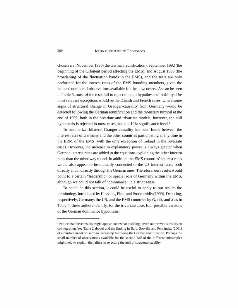
chosen are: November 1990 (the German reunification), September 1992 (the

beginning of the turbulent period affecting the EMS), and August 1993 (the

broadening of the fluctuation bands in the EMS), and the tests are only

performed for the interest rates of the EMS founding members, given the

reduced number of observations available for the newcomers. As can be seen

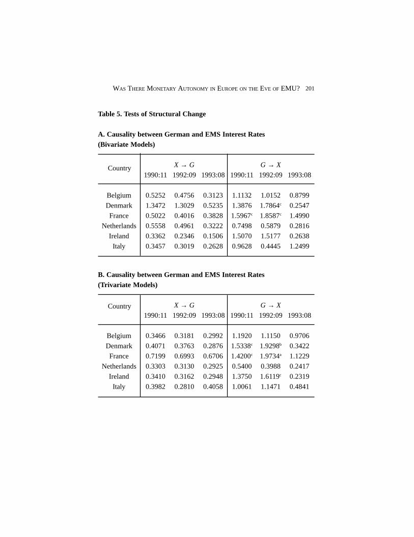
in Table 5, most of the tests fail to reject the null hypothesis of stability. The

most relevant exceptions would be the Danish and French cases, where some

signs of structural change in Granger-causality from Germany would be

detected following the German reunification and the monetary turmoil at the

end of 1992, both in the bivariate and trivariate models; however, the null

hypothesis is rejected in most cases just at a 10% significance level.4

To summarize, bilateral Granger-causality has been found between the

interest rates of Germany and the other countries participating at any time in

the ERM of the EMS (with the only exception of Ireland in the bivariate

case). However, the increase in explanatory power is always greater when

German interest rates are added to the equations explaining the other interest

rates than the other way round. In addition, the EMS countries’ interest rates

would also appear to be mutually connected to the US interest rates, both

directly and indirectly through the German ones. Therefore, our results would

point to a certain “leadership” or special role of Germany within the EMS,

although we could not talk of “dominance” in a strict sense.

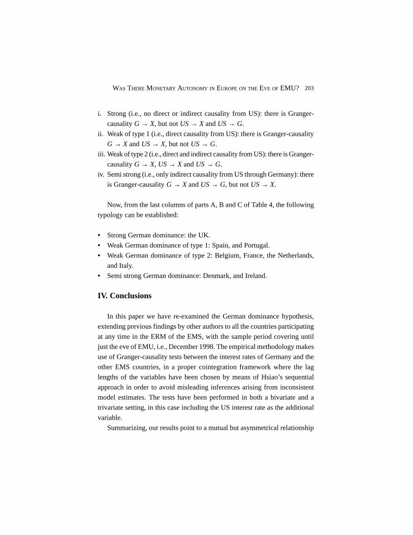
To conclude this section, it could be useful to apply to our results the

terminology introduced by Hassapis, Pittis and Prodromidis (1999). Denoting,

respectively, Germany, the US, and the EMS countries by G, US, and X as in

Table 4, these authors identify, for the trivariate case, four possible versions

of the German dominance hypothesis:

4 Notice that these results might appear somewhat puzzling, given our previous results oncointegration (see Table 2 above) and the finding in Bajo, Sosvilla and Fernández (2001)of a reinforcement of German leadership following the German reunification. Perhaps thesmall number of observations available for the second half of the different subsamplesmight help to explain the failure in rejecting the null of structural stability.


Table 5. Tests of Structural Change

A. Causality between German and EMS Interest Rates(Bivariate Models)

X → G G → X

1990:11 1992:09 1993:08 1990:11 1992:09 1993:08

Belgium 0.5252 0.4756 0.3123 1.1132 1.0152 0.8799

Denmark 1.3472 1.3029 0.5235 1.3876 1.7864c 0.2547

France 0.5022 0.4016 0.3828 1.5967c 1.8587c 1.4990

Netherlands 0.5558 0.4961 0.3222 0.7498 0.5879 0.2816

Ireland 0.3362 0.2346 0.1506 1.5070 1.5177 0.2638

Italy 0.3457 0.3019 0.2628 0.9628 0.4445 1.2499

B. Causality between German and EMS Interest Rates(Trivariate Models)

X → G G → X

1990:11 1992:09 1993:08 1990:11 1992:09 1993:08

Belgium 0.3466 0.3181 0.2992 1.1920 1.1150 0.9706

Denmark 0.4071 0.3763 0.2876 1.5338c 1.9298b 0.3422

France 0.7199 0.6993 0.6706 1.4200c 1.9734a 1.1229

Netherlands 0.3303 0.3130 0.2925 0.5400 0.3988 0.2417

Ireland 0.3410 0.3162 0.2948 1.3750 1.6119c 0.2319

Italy 0.3982 0.2810 0.4058 1.0061 1.1471 0.4841

Country

Country


C. Causality between US and EMS Interest Rates(Trivariate Models)

X → US US → X

1990:11 1992:09 1993:08 1990:11 1992:09 1993:08

Belgium 0.7614 0.4571 0.4153 1.1452 1.1778 1.0222

Denmark 1.2914 0.8780 0.6659 1.3542 1.6384c 0.2384

France 1.1509 0.7850 0.4990 1.5068 1.3741 0.7552

Netherlands 0.6850 0.5462 0.5179 0.5464 0.4176 0.2485

Ireland 0.9324 0.5884 0.4063 1.3750 1.6119 0.2319

Italy 1.2955 0.5716 0.4139 1.0061 1.1471 0.4841

D. Causality between US and German Interest Rates(Trivariate Models)

G → US US → G

1990:11 1992:09 1993:08 1990:11 1992:09 1993:08

Belgium 1.0792 0.6449 0.6312 0.5701 0.6168 0.3963

Denmark 1.2914 0.8780 0.6659 0.9298 0.9003 0.4341

France 0.8817 0.4799 0.4143 0.6514 0.6230 0.6146

Netherlands 0.8018 0.6017 0.6175 0.5851 0.5924 0.3112

Ireland 0.8364 0.6048 0.4118 0.6697 0.4268 0.4100

Italy 1.0824 0.4630 0.3363 0.4374 0.4408 0.2775

Notes: X , G, and US denote every country in the first column of the tables, Germany andthe US, respectively. (a), (b), and (c) denote significance at the 1%, 5%, and 10% levels,

respectively.

Country

Country


i. Strong (i.e., no direct or indirect causality from US): there is Granger-

causality G → X, but not US → X and US → G.

ii. Weak of type 1 (i.e., direct causality from US): there is Granger-causality

G → X and US → X, but not US → G.

iii. Weak of type 2 (i.e., direct and indirect causality from US): there is Granger-

causality G → X, US → X and US → G.

iv. Semi strong (i.e., only indirect causality from US through Germany): there

is Granger-causality G → X and US → G, but not US → X.

Now, from the last columns of parts A, B and C of Table 4, the following

typology can be established:

• Strong German dominance: the UK.

• Weak German dominance of type 1: Spain, and Portugal.

• Weak German dominance of type 2: Belgium, France, the Netherlands,

and Italy.

• Semi strong German dominance: Denmark, and Ireland.

IV. Conclusions

In this paper we have re-examined the German dominance hypothesis,

extending previous findings by other authors to all the countries participating

at any time in the ERM of the EMS, with the sample period covering until

just the eve of EMU, i.e., December 1998. The empirical methodology makes

use of Granger-causality tests between the interest rates of Germany and the

other EMS countries, in a proper cointegration framework where the lag

lengths of the variables have been chosen by means of Hsiao’s sequential

approach in order to avoid misleading inferences arising from inconsistent

model estimates. The tests have been performed in both a bivariate and a

trivariate setting, in this case including the US interest rate as the additional

variable.

Summarizing, our results point to a mutual but asymmetrical relationship


between Germany and the other countries participating at any time in the

ERM of the EMS, since bilateral Granger-causality was found between the

interest rates of Germany and those of the other countries, although the German

interest rates added more to the explanation of the other interest rates than in

the opposite case. Also, a mutual connection between the EMS countries’

and the US interest rates would emerge, both directly and indirectly through

the German rates. Finally, we hardly found evidence of significant structural

changes in the estimated relationships following the German reunification,

the monetary turmoil at the end of 1992, and the broadening of the fluctuation

bands in the EMS.

Therefore, our results would support a weak version of the hypothesis of

German dominance during the working of the EMS, since there would have

prevailed a mutual relationship among the monetary policies of all the countries

involved, even though that relationship would have been stronger from

Germany to the other countries than in the opposite way. Then, Germany

would have played a certain “leadership” or special role in the EMS, although

she would not have been strictly the “dominant” player.

Regarding the policy implications of the paper, these would provide some

mild support to the hypothesis about EMU as an economic response to the

loss of monetary autonomy in Europe in favor of Germany, especially after

the achievement of full capital mobility in the first nineties (Wyplosz, 1997).

Also, the position of the Mediterranean countries (Italy, Spain, and Portugal)

faced to EMU does not seem to be too different to that of the “core” European

countries, at least in terms of the autonomy of their monetary policies before

EMU. The same can be said for Denmark and the UK, two countries that

chose not to participate in EMU; in fact, and somewhat ironically, the UK

would have been, according to our results, the country most “dominated” by

German monetary policy actions.

References

Bajo-Rubio, O., Sosvilla-Rivero, S. and F. Fernández-Rodríguez (2001),


“Asymmetry in the EMS: New Evidence Based on Non-Linear Forecasts,”European Economic Review 45: 451-473.

Camarero, M., Esteve, V. and C. Tamarit (1997), “Convergencia en Tipos deInterés de la Economía Española ante la Unión Monetaria Europea,”

Revista de Análisis Económico 12: 71-99.Caporale, G.M. and N. Pittis (1995), “Interest Rate Linkages within the

European Monetary System: An Alternative Interpretation,” Applied

Economics Letters 2: 45-47.

Cohen, D. and C. Wyplosz (1989), “The European Monetary Union: AnAgnostic Evaluation,” in R. Bryant et al. (eds.), Macroeconomic Policies

in an Interdependent World, Washington, DC, International MonetaryFund: 311-337.

De Grauwe, P. (2000), Economics of Monetary Union (4th edition), Oxford,Oxford University Press.

Engle, R.F. and C.W.J. Granger (1987), “Co-integration and Error Correction:Representation, Estimation and Testing,” Econometrica 55: 251-276.

Gardner, E. and W. Perraudin (1993), “Asymmetry in the ERM: A Case Studyof French and German Interest Rates before and after German Unification,”

International Monetary Fund Staff Papers 40: 427-450.Giavazzi, F. and A. Giovannini (1987), “Models of the EMS: Is Europe a

Greater Deutschmark Area?,” in R. Bryant and R. Portes (eds.), Global

Macroeconomics. Policy Conflict and Cooperation, London, Macmillan:

237-265.Giavazzi, F. and A. Giovannini (1989), Limiting Exchange Rate Flexibility.

The European Monetary System, Cambridge, MA, The MIT Press.Giavazzi, F. and M. Pagano (1988), “The Advantage of Tying One’s Hands.

EMS Discipline and Central Bank Credibility,” European Economic

Review 32: 1055-1075.

Granger, C.W.J. (1969), “Investigating Causal Relations by EconometricModels and Cross-Spectral Methods,” Econometrica 37: 424-438.

Hassapis, C., Pittis, N. and K. Prodromidis (1999), “Unit Roots and GrangerCausality in the EMS Interest Rates: The German Dominance Hypothesis

Revisited,” Journal of International Money and Finance 18: 47-73.


Henry, J. and J. Weidmann (1995), “Asymmetry in the EMS Revisited:

Evidence from the Causality Analysis of Daily Eurorates,” Annales

d'Économie et de Statistique 40: 125-160.

Hsiao, C. (1981), “Autoregressive Modelling and Money-Income Causality

Detection,” Journal of Monetary Economics 7: 85-106.

Karfakis, C. and D. Moschos (1990), “Interest Rate Linkages within the

European Monetary System: A Time Series Analysis,” Journal of Money,

Credit, and Banking 22: 388-394.

Katsimbris, G. and S. Miller (1993), “Interest Rate Linkages within the

European Monetary System: Further Analysis,” Journal of Money, Credit,

and Banking 25: 771-779.

Koedijk, K. and C. Kool (1992), “Dominant Interest and Inflation Differentials

within the EMS,” European Economic Review 36: 925-943.

Kwiatkowski, D., Phillips, P.C.B., Schmidt, P. and Y. Shin (1992), “Testing

the Null Hypothesis of Stationarity against the Alternative of a Unit Root.

How Sure Are We that Economic Time Series Have a unit Root?,” Journal

of Econometrics 54: 159-178.

MacKinnon, J.G. (1991), “Critical Values for Cointegration Tests,” in R.F.

Engle and C.W.J. Granger (eds.), Long-run Economic Relationships:

Readings in Cointegration, Oxford, Oxford University Press: 267-276.

Mélitz, J. (1988), “Monetary Discipline and Cooperation in the European

Monetary System: A Synthesis,” in F. Giavazzi, S. Micossi and M. Miller

(eds.), The European Monetary System, Cambridge, Cambridge University

Press: 51-79.

Phillips, P.C.B. and P. Perron (1988), “Testing for a Unit Root in Time Series

Regression,” Biometrika 75: 335-346.

Shin, Y. (1994), “A Residual-Based Test of the Null of Cointegration against

the Alternative of no Cointegration,” Econometric Theory 10: 91-115.

Stock, J.H. and M.W. Watson (1993), “A Simple Estimator of Cointegrating

Vectors in Higher Order Integrated Systems,” Econometrica 61: 783-820.

Von Hagen, J. and M. Fratianni (1990), “German Dominance in the EMS:


Evidence from Interest Rates,” Journal of International Money and

Finance 9: 358-375.

Wyplosz, C. (1997), “EMU: Why and how it might Happen,” Journal of

Economic Perspectives 11: 3-21.

Documents

W AS THERE MONETARY AUTONOMY IN EUROPE ON · PDF fileW AS THERE MONETARY AUTONOMY IN EUROPE ON ... the loss of monetary autonomy in Europe ... began to circulate and replaced the old