Embed Size (px)
Citation preview
Contents
The Mumford conjecture, Madsen-Weiss and homological stabilityfor mapping class groups of surfaces
Nathalie Wahl 1
The Mumford conjecture, Madsen-Weiss and homological stability for mappingclass groups of surfaces 3
Introduction 3
Lecture 1. The Mumford conjecture and the Madsen-Weiss theorem 51. The Mumford conjecture 52. Moduli space, mapping class groups and diffeomorphism groups 53. The Mumford-Morita-Miller classes 74. Homological stability 75. The Madsen-Weiss theorem 96. Exercices 10
Lecture 2. Homological stability: geometric ingredients 111. General strategy of proof 112. The case of the mapping class group of surfaces 113. The ordered arc complex 124. Curve complexes and disc spaces 155. Exercices 15
Lecture 3. Homological stability: the spectral sequence argument 171. Double complexes associated to actions on simplicial complexes 172. The spectral sequence associated to the horizontal filtration 183. The spectral sequence associated to the vertical filtration 184. The proof of stability for surfaces with boundaries 195. Closing the boundaries 216. Exercises 21
Lecture 4. Homological stability: the connectivity argument 231. Strategy for computing the connectivity of the ordered arc complex 232. Contractibility of the full arc complex 243. Deducing connectivity of smaller complexes 254. Exercises 26
Bibliography 27
i

The Mumford conjecture,Madsen-Weiss and homological
stability for mapping class groupsof surfaces
Nathalie Wahl

IAS/Park City Mathematics SeriesVolume XX, XXXX
The Mumford conjecture, Madsen-Weiss andhomological stability for mapping class groups of
surfaces
Nathalie Wahl
Introduction
The Mumford conjecture [26] says that the rational cohomology ring of the mod-uli space of Riemann surfaces is a polynomial algebra on the so-called Mumford-Morita-Miller classes, in a range of degrees increasing with the genus of the surface.This conjecture is now known to be true, using the following two theorems as mainingredients: Harer’s stability theorem [16] which tells us that the rational coho-mology of the moduli space is independent of the genus in a range of dimensions,and Madsen-Weiss’ theorem [23] which identifies the stable cohomology with thatpolynomial algebra.
Harer’s and Madsen-Weiss’ theorems are both statements about the integralhomology of the mapping class groups of surfaces, using, in the Madsen-Weiss’ case,Earl and Eells’ theorem [8] relating the diffeomorphism groups to the mapping classgroups of surfaces. In Lecture 1, we describe the relationship between the modulispace of Riemann surfaces, the mapping class groups and the diffeomorphism groupsof surfaces. We then give a definition of the Mumford-Morita-Miller classes, statethe main part of Harer’s stability theorem, and give a first statement of Madsen-Weiss’ theorem.
The last three lectures are devoted to a sketch proof of Harer stability theorem,using improvements by Ivanov [19, 20], Hatcher [17], Boldsen [4] and Randal-Williams [32]. This proof uses two spectral sequences associated to the action ofthe mapping class groups on certain simplicial complexes of arcs in the surfaces.In Lecture 2, we give the general strategy, define the relevant arc complexes andstudy the properties of the action of the mapping class groups on these complexes.In Lecture 3, we give the spectral sequence argument (following Randal-Williams).Harer’s stability theorem is proved by studying the spectral sequences carefully,using the properties of the action given in Lecture 2, as well as a connectivityproperty of the arc complexes, whose proof is sketched in Lecture 4. The last threeare mostly based on the survey [37].
This series of lectures is supplemented by Galatius’ lectures in this volume [11],which present a sketch proof of the Madsen-Weiss theorem.
University of CopenhagenE-mail address: [email protected] by the Danish National Sciences Research Council (DNSRC) and the European Re-
search Council (ERC), as well as by the Danish National Research Foundation (DNRF) throughthe Centre for Symmetry and Deformation.
c©2011 American Mathematical Society
3

LECTURE 1
The Mumford conjecture and the Madsen-Weisstheorem
In this lecture, we give a brief introduction to important players in the proofof the Mumford conjecture by Madsen and Weiss. We introduce the moduli spaceof Riemann surface, the Teichmuller space and describe their relationship to dif-feomorphism groups and mapping class groups of surfaces. We state the Mumfordconjecture, the Madsen-Weiss theorem and Harer’s stability theorem.
1. The Mumford conjecture
Let Sg be a closed, smooth, oriented surface of genus g and let Diff(Sg) denotethe topological group of orientation preserving diffeomorphisms of Sg. The modulispace Mg can be defined in many ways:
Mg = Moduli space of Riemann surfaces= Space of conformal classes of Riemannian metrics on Sg= Riemannian metrics on Sg/Diff(Sg)= Isometry classes of hyperbolic structures on Sg= Biholomorphic classes of complex structures on Sg= Isomorphy classes of smooth algebraic curves homeomorphic to Sg
We would like to describe Mg, and, for example, compute its (co)homology.The present lectures, together with Galatius’ lectures in the same volume [11], arecentered around the following result about Mg:
Theorem 1.1 (Mumford conjecture, proved by Madsen-Weiss [23, 26]).
H∗(Mg; Q) ∼=(∗) Q[κ1, κ2, . . . ] with |κi| = 2i
where the isomorphism (∗) is in a range of dimension growing with g.
We will reformulate this theorem in terms of diffeomorphism groups and map-ping class groups of surfaces. The classes κi are called the Mumford-Morita-Millerclasses and are defined below, and the range for the isomorphism is the homologicalstability range of the mapping class group of surfaces, also given explicitly below.
2. Moduli space, mapping class groups and diffeomorphism groups
Define the Teichmuller space
Tg = Riemannian metrics on Sg/Diff0(Sg)with Diff0(Sg) the topological group of diffeomorphisms of Sg isotopic to the iden-tity, i.e. the component of the identity in Diff(Sg), acting on the space of metricsby pull-back (see [9, 10.1]).
5
6 NATHALIE WAHL, MUMFORD CONJECTURE, MADSEN-WEISS AND STABILITY
Let
Γg = Γ(Sg) := Diff(Sg)/Diff0(Sg) = π0 Diff(Sg)
denote the mapping class group of Sg. (We note that Γg is also often denotedMod(Sg), and sometimes refered to as the modular group.) The group Γg acts onTg, via the full action of Diff(Sg) on the space of metrics (see [9, 12.1]), and
Mg = Tg/Γg
As Tg ' ∗ (in fact Tg ∼= R6g−6, see [9, 10.6]) and Γg acts properly discontinu-ously on Tg with finite stabilizers [9, 12.1,12.3], we have
H∗(Mg; Q) ∼= H∗(BΓg; Q)
where BΓg is a classifying space for Γg, i.e. BΓg = EΓg/Γg, for EΓg ' ∗ with freeproperly discontinuous Γg–action. [See exercices after Lecture 3.]
Recall moreover that H∗(BΓg; Z) = H∗(Γg; Z) is the group cohomology of Γg(see [5, I.4]).
To relate these homology groups to the diffeomorphism group, we need thefollowing
Theorem 1.2 (Earl-Eells [8]). For g ≥ 2, Diff(Sg) has contractible components.
In other words, the theorem says that the homomorphism
Diff(Sg)→ π0 Diff(Sg) = Γg
is a homotopy equivalence. As one can build compatible models of EDiff(Sg) andEΓg (via the standard resolution and a topological version of it [5, I.5]), it followsthat, when g ≥ 2,
BDiff(Sg) = EDiff(Sg)/Diff(Sg)'−→ EΓg/Γg = BΓg
and thus
H∗(Mg; Q) ∼= H∗(Γg; Q) ∼= H∗(BΓg; Q) ∼= H∗(BDiff(Sg); Q)
giving us many formulations of the Mumford conjecture.
The space BDiff(Sg) is a classifying space for Sg-bundles: there is a 1-1 corre-spondence
Sg → Eπ→ X/∼= ←→ Maps(X,BDiff(Sg))/'
between isomorphism classes of bundles and homotopy classes of maps. Moreover,elements of H∗(BDiff(Sg)) are characteristic classes for Sg–bundles: they give anassignment of a cohomology class c(E, π) ∈ H∗(X) to any bundle Sg → E
π→X, which is natural in the sense that c(g∗(E, π)) = g∗c(E, π) for any map g :Y → X. Given a class c ∈ H∗(BDiff(Sg)), the associated characteristic class isdefined by c(E, π) = f∗(c) for f : X → BDiff(Sg) classifying (E, π) via the abovecorrespondence. (See [11, Cor 1.5,1.6] for more details, using an embedding modelfor BDiff(Sg).)
LECTURE 1. THE MUMFORD CONJECTURE AND THE MADSEN-WEISS THEOREM 7
3. The Mumford-Morita-Miller classes
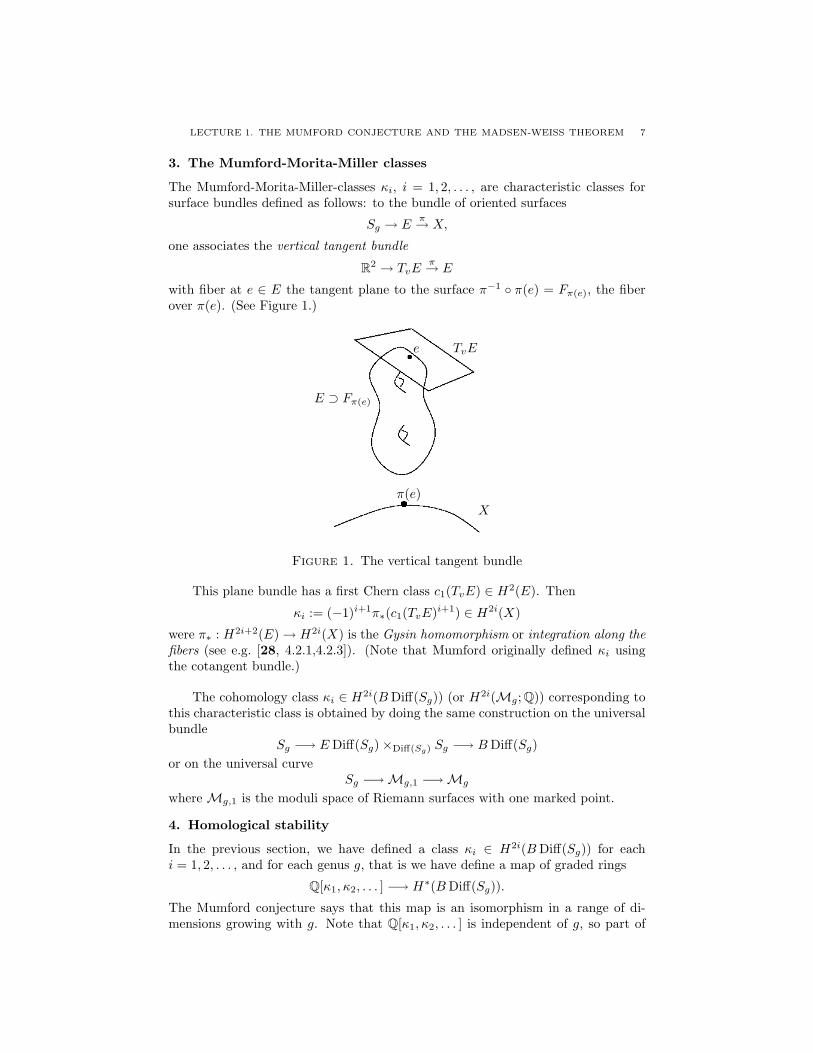
The Mumford-Morita-Miller-classes κi, i = 1, 2, . . . , are characteristic classes forsurface bundles defined as follows: to the bundle of oriented surfaces
Sg → Eπ→ X,
one associates the vertical tangent bundle
R2 → TvEπ→ E
with fiber at e ∈ E the tangent plane to the surface π−1 π(e) = Fπ(e), the fiberover π(e). (See Figure 1.)
e
π(e)
E ⊃ Fπ(e)
X
TvE
Figure 1. The vertical tangent bundle
This plane bundle has a first Chern class c1(TvE) ∈ H2(E). Then
κi := (−1)i+1π∗(c1(TvE)i+1) ∈ H2i(X)
were π∗ : H2i+2(E)→ H2i(X) is the Gysin homomorphism or integration along thefibers (see e.g. [28, 4.2.1,4.2.3]). (Note that Mumford originally defined κi usingthe cotangent bundle.)
The cohomology class κi ∈ H2i(BDiff(Sg)) (or H2i(Mg; Q)) corresponding tothis characteristic class is obtained by doing the same construction on the universalbundle
Sg −→ EDiff(Sg)×Diff(Sg) Sg −→ BDiff(Sg)or on the universal curve
Sg −→Mg,1 −→Mg
where Mg,1 is the moduli space of Riemann surfaces with one marked point.
4. Homological stability
In the previous section, we have defined a class κi ∈ H2i(BDiff(Sg)) for eachi = 1, 2, . . . , and for each genus g, that is we have define a map of graded rings
Q[κ1, κ2, . . . ] −→ H∗(BDiff(Sg)).
The Mumford conjecture says that this map is an isomorphism in a range of di-mensions growing with g. Note that Q[κ1, κ2, . . . ] is independent of g, so part of
8 NATHALIE WAHL, MUMFORD CONJECTURE, MADSEN-WEISS AND STABILITY
the Mumford conjecture is a stability statement, which says that the cohomology ofMg in any given degree is independent of g if g is sufficiently large. This is knownas Harer’s stability theorem, which we state in this section.
A familly of groups
G1 → G2 → . . . → Gn → . . .
satisfies homological stability if the induced maps
Hi(Gn) −→ Hi(Gn+1)
are isomorphisms in a range i n, where H∗(Gn) denotes the group homology ofGn.
Examples: Families of groups satisfying homological stability are Gn = the sym-metric group Σn [29], the braid group βn [1], the linear group GLn(Z) [13].
Define G∞ =⋃n≥1Gn to be the “stable group”. If Gnn≥1 satisfies homolog-
ical stability, then
Hi(Gn) ∼= Hi(G∞) in the range i n
and H∗(G∞) is the “stable homology”.
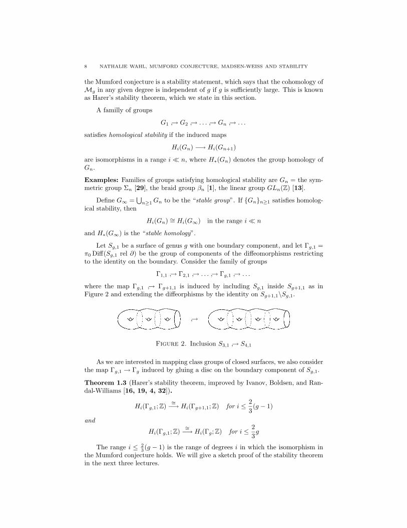
Let Sg,1 be a surface of genus g with one boundary component, and let Γg,1 =π0 Diff(Sg,1 rel ∂) be the group of components of the diffeomorphisms restrictingto the identity on the boundary. Consider the family of groups
Γ1,1 → Γ2,1 → . . . → Γg,1 → . . .
where the map Γg,1 → Γg+1,1 is induced by including Sg,1 inside Sg+1,1 as inFigure 2 and extending the diffeorphisms by the identity on Sg+1,1\Sg,1.
→
Figure 2. Inclusion S3,1 → S4,1
As we are interested in mapping class groups of closed surfaces, we also considerthe map Γg,1 → Γg induced by gluing a disc on the boundary component of Sg,1.
Theorem 1.3 (Harer’s stability theorem, improved by Ivanov, Boldsen, and Ran-dal-Williams [16, 19, 4, 32]).
Hi(Γg,1; Z)∼=−→ Hi(Γg+1,1; Z) for i ≤ 2
3(g − 1)
and
Hi(Γg,1; Z)∼=−→ Hi(Γg; Z) for i ≤ 2
3g
The range i ≤ 23 (g − 1) is the range of degrees i in which the isomorphism in
the Mumford conjecture holds. We will give a sketch proof of the stability theoremin the next three lectures.
LECTURE 1. THE MUMFORD CONJECTURE AND THE MADSEN-WEISS THEOREM 9
5. The Madsen-Weiss theorem
The Madsen-Weiss theorem gives a computation of the stable (co)homology ofmapping class groups, i.e. the group (co)homology of
Γ∞ =⋃g≥1
Γg,1
or singular (co)homology of its classifying space BΓ∞. We give now a first formu-lation of this theorem, without defining all the players yet:
Theorem 1.4 (Madsen-Weiss [23]). There is a homology isomorphism
BΓ∞ −→ Ω∞0 MTSO(2)
where the target is the 0th component of the infinite loop space of the spectrumMTSO(2).
The spectrum MTSO(2), defined in Galatius’ lectures [11], is build out ofGrassmanians of 2-planes in Rn, in the limit as n → ∞, and the map uses avertical tangent bundle type construction. (See Definition 1.7, Theorem 1.8 andCorollary 1.10 in [11].)
Using homological stability, this can be restated as saying that
Hi(Γg; Z) ∼= Hi(Ω∞MTSO(2); Z) for i ≤ 23
(g − 1)
(and the same for cohomology using the universal coefficient theorem).The target space is computable and H∗(Ω∞0 MTSO(2); Q) = Q[κ1, κ2, . . . ] with
κi in degree 2i corresponding to the Mumford-Morita-Miller-class of the same name(see [11, 2.1]). Combining these two facts gives the Mumford conjecture, namelythat
H∗(Mg; Q) ∼= H∗(Γg,Q) ∼=(∗) Q[κ1, κ2, . . . ]where the isomorphism (∗) is up to degree 2
3 (g − 1).
This type of theorem for the symmetric groups and braid groups were alreadyproved in the early 70’s:
Theorem 1.5 (Symmetric groups). H∗(Σ∞) ∼= H∗(Ω∞0 S∞)
Theorem 1.6 (Braid groups). H∗(β∞) ∼= H∗(Ω20S
2)
The first theorem is known as the Barratt-Priddy theorem [31]. Both theoremscan be seen as special cases of the approximation theorem, which says that the mapCnX → ΩnΣnX is a group completion for Cn the little n-cubes monad. Here oneneeds to take X = S0 and n = ∞ in the first case, and the same X but n = 2in the second case. (See May [24, Thm 2.7] and [7, p.486 (15)], or Segal [35,Thm 1], for the approximation theorem—see also the work of Boardman-Vogt [3]and Barratt-Eccles [2]. See [11, Lec 4] or [25] for the group completion theorem.)The proof of the Madsen-Weiss Theorem presented in Galatius’ lecture series [11]follows Galatius–Randal-Williams [12], which can be seen as a generalization ofSegal’s proof of the approximation theorem.
The Madsen-Weiss Theorem was generalized to other types of mapping classgroups of surfaces (Non-orientable [36], framed, Spin and Pin mapping class groups[33]). Other examples are
Theorem 1.7 (Automorphisms of free groups [10]). H∗(Aut∞) ∼= H∗(Ω∞0 S∞)
10 NATHALIE WAHL, MUMFORD CONJECTURE, MADSEN-WEISS AND STABILITY
Here Aut∞ =⋃n≥1 Aut(Fn) with Fn the free group on n letters.
Theorem 1.8 (Handlebody groups [18]). H∗(H∞) ∼= H∗(Ω∞0 Σ∞(BSO(3)+))
Here H∞ =⋃g≥1Hg,1 with Hg,1 = π0 Diff(Hg rel D2) the mapping class group
of a handlebody Hg of genus g fixing a disc in the boundary of Hg.All the above examples are computations of the homology of the stable group
of a family of groups satisfying homological stability, so they all can be restatedas computations of the homology of the unstable groups in a range of degrees.Stability is however not a necessary ingredient of a “Madsen-Weiss theorem”—it israther an interpretational tool.
6. Exercices
1) Show that S2 and T 2 do not satisfy the Earl-Eells theorem, i.e. that Diff(S2)and Diff(T 2) do not have contractible components.
2) Give a definition of the group Γ∞ =⋃g≥1 Γg,1 in terms of an infinite genus
surface S∞.3) Let Γ1
g = π0 Diff(S1g) denote the mapping class group of a once punctured genus g
surface S1g . Use homological stability and a factorization of the map Γg,1 → Γg,0
to show injectivity of the map Hi(Γg,1)→ Hi(Γ1g) in a range.
LECTURE 2
Homological stability: geometric ingredients
In this lecture, we briefly describe a general strategy for proving homologicalstability for families of groups and then give the main geometric ingredients neededfor the case of the mapping class group of surfaces, with an emphasis on the caseof surfaces with boundaries. We follow Randal-Williams [32] and the survey [37],which contains further details.
1. General strategy of proof
A simplicial complex X = (X0,F) is a set of vertices X0 together with a collectionF of subsets of X0 closed under taking subsets and containing all the singletons.The subsets of cardinality p+ 1 are called the p–simplices of X.
To a simplicial complex X, one can associate its realization |X| which has atopological p-simplex ∆p for each p-simplex of X.
A space or simplicial complex X is called n–connected if πi(X) = 0 for all i ≤ n(where πi(X) := πi(|X|) if X is a simplicial complex). Note that, by Hurewicztheorem, a simply connected space X is n-connected, n ≥ 2, if and only if H∗(X) =0 for 2 ≤ ∗ ≤ n.
Given a familly of groups
G1 → G2 → . . . → Gn → . . .
we want to find a simplicial complex (or simplicial set) Xn for each n such that
• Gn acts on Xn,• the stabilizer Stab(σp) ∼= Gn−p−1 for any p-simplex σp,• the action is as transitive as possible,• Xn is highly connected.
There is then a spectral sequence for the action of Gn on Xn which decomposes thehomology of Gn in terms of the homology of the stabilizers. As these are assumedto be previous groups in the sequence, this spectral sequence allows an inductiveargument. (See Lecture 3 for more details.)
2. The case of the mapping class group of surfaces
To prove homological stability for the groups Γg, we will need to consider surfaceswith any number of boundary components. Let S = Sg,r be a surface of genus gwith r boundary components. We will consider 3 maps
αg : Γ(Sg,r) → Γ(Sg+1,r−1)βg : Γ(Sg,r) → Γ(Sg,r+1)δg : Γ(Sg,r) → Γ(Sg,r−1)
11
12 NATHALIE WAHL, MUMFORD CONJECTURE, MADSEN-WEISS AND STABILITY
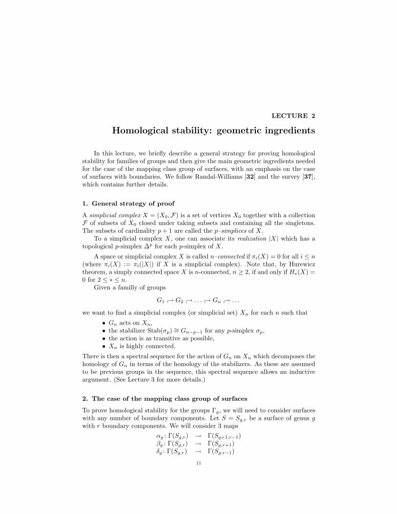
αβ δ
Figure 1. The maps α, β and δ
induced by gluing a strip which identifies arcs lying in different (for α) or the same(for β) boundary component(s) of S, and by gluing a disc (for δ). (See Figure 1.)
The proof of homological stability for mapping class groups presented hereinvolves three simplicial spaces: an arc complex for each of α and β, and a discspace for δ. In the remainer of the lecture, we will define the two arc complexesand study their properties. These are the complexes O2 and O1 defined below.
3. The ordered arc complex
We will work here with collections of disjointly embedded arcs in a surface. We saythat a collection of arcs 〈a0, . . . , ap〉 is non-separating if its complement S\(a0 ∪· · · ∪ ap) is connected.
Given a surface S with points b0, b1 in its boundary, define O(S, b0, b1) to bethe simplicial complex with
vertices =: isotopy classes of non-separating arcs with boundary b0, b1p–simplices =: non-separating collections of p + 1 distinct isotopy classes
of arcs 〈a0, . . . , ap〉 disjointly embeddable (away from b0, b1) in such away that the anticlockwise ordering of a0, . . . , ap at b0 agrees with theclockwise ordering at b1.
Up to isomorphism, there are two such complexes:O1(S) =: O(S, b0, b1) with b0, b1 on the same boundary component,O2(S) =: O(S, b0, b1) with b0, b1 on different boundary components.
The mapping class group Γ(Sg,r) = Γg,r acts on O1(Sg,r) and O2(Sg,r). Wegive now the properties of this action that are key for us.
Property 1. Γ(S) acts transitively on p–simplices of Oi(S) for each p.
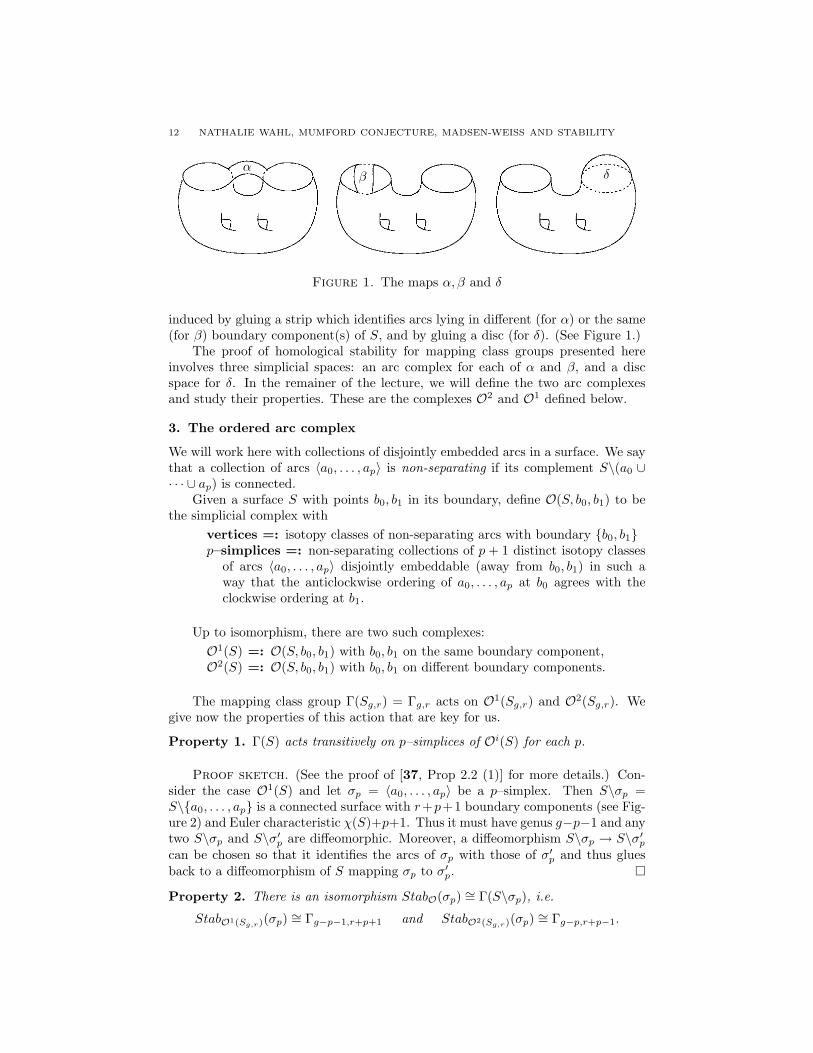
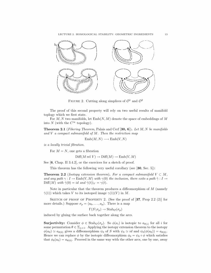
Proof sketch. (See the proof of [37, Prop 2.2 (1)] for more details.) Con-sider the case O1(S) and let σp = 〈a0, . . . , ap〉 be a p–simplex. Then S\σp =S\a0, . . . , ap is a connected surface with r+p+1 boundary components (see Fig-ure 2) and Euler characteristic χ(S)+p+1. Thus it must have genus g−p−1 and anytwo S\σp and S\σ′p are diffeomorphic. Moreover, a diffeomorphism S\σp → S\σ′pcan be chosen so that it identifies the arcs of σp with those of σ′p and thus gluesback to a diffeomorphism of S mapping σp to σ′p.
Property 2. There is an isomorphism StabO(σp) ∼= Γ(S\σp), i.e.
StabO1(Sg,r)(σp) ∼= Γg−p−1,r+p+1 and StabO2(Sg,r)(σp) ∼= Γg−p,r+p−1.
LECTURE 2. HOMOLOGICAL STABILITY: GEOMETRIC INGREDIENTS 13
b0 b1
b0 b1
Figure 2. Cutting along simplices of O1 and O2
The proof of this second property will rely on two useful results of manifoldtoplogy which we first state.
For M,N two manifolds, let Emb(N,M) denote the space of embeddings of Minto N (with the C∞ topology).
Theorem 2.1 (Fibering Theorem, Palais and Cerf [30, 6]). Let M,N be manifoldsand V a compact submanifold of M . Then the restriction map
Emb(M,N) −→ Emb(V,N)
is a locally trivial fibration.
For M = N , one gets a fibration
Diff(M rel V )→ Diff(M)→ Emb(V,M)
See [6, Chap. II 3.4.2], or the exercices for a sketch of proof.
This theorem has the following very useful corollary (see [30, Sec. 5]):
Theorem 2.2 (Isotopy extension theorem). For a compact submanifold V ⊂ M ,and any path γ : I → Emb(V,M) with γ(0) the inclusion, there exits a path γ : I →Diff(M) with γ(0) = id and γ(t)|V = γ(t).
Note in particular that the theorem produces a diffeomorphism of M (namelyγ(1)) which takes V to its isotoped image γ(1)(V ) in M .
Sketch of proof of Property 2. (See the proof of [37, Prop 2.2 (2)] formore details.) Suppose σp = 〈a0, . . . , ap〉. There is a map
Γ(S\σp)→ StabO(σp)
induced by gluing the surface back together along the arcs.
Surjectivity: Consider φ ∈ StabO(σp). So φ(ai) is isotopic to aθ(i) for all i forsome permutation θ ∈ Σn+1. Applying the isotopy extension theorem to the isotopyφ(a0) ' aθ(0) gives a diffeomorphism ψ0 of S with ψ0 ' id and ψ0(φ(a0)) = aθ(0).Hence we can replace φ by the isotopic diffeomorphism φ0 = ψ0 φ which satisfiesthat φ0(a0) = aθ(0). Proceed in the same way with the other arcs, one by one, away
14 NATHALIE WAHL, MUMFORD CONJECTURE, MADSEN-WEISS AND STABILITY
from the arcs already dealt with. Hence we can replace φ with a diffeomorphismthat fixes the arcs, possibly up to a permutation. But the permutation must betrivial as φ fixes the boundary. Then φ can be reinterpreted as a diffeomorphismof S\σp.
Injectivity: Suppose p = 0 for simplicity. We would like to show that the mapΓ(S\I) → Γ(S) is injective for any (non-separating) arc I. A relative version ofTheorem 2.1 above gives a fibration
Diff(S rel ∂S ∪ I)→ Diff(S rel ∂S)→ Emb∂(I, S)
where Emb∂(I, S) denotes the space of embeddings of an arc I in S with ∂I mappingto chosen points A,B ∈ ∂S. By [15, Thm 5], each component of Emb∂(I, S) iscontractible. The result then follows from looking at the long exact sequence ofhomotopy groups of the fibration for the component of the non-separating arcs.
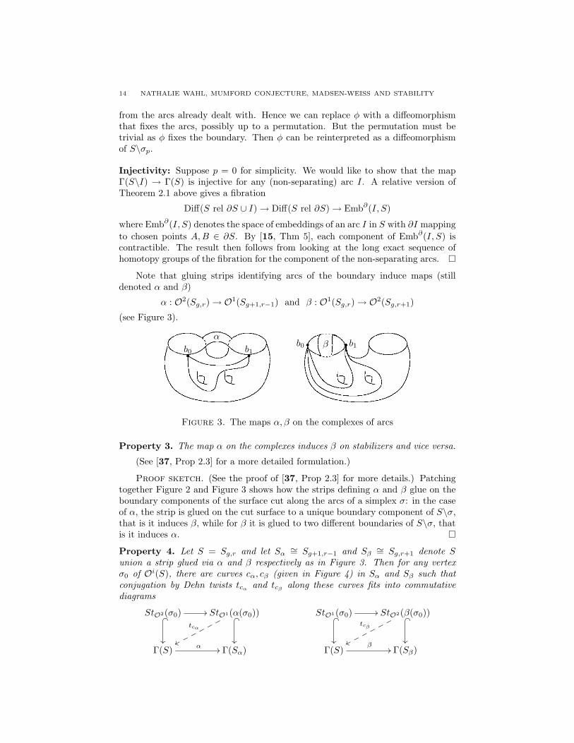
Note that gluing strips identifying arcs of the boundary induce maps (stilldenoted α and β)
α : O2(Sg,r)→ O1(Sg+1,r−1) and β : O1(Sg,r)→ O2(Sg,r+1)
(see Figure 3).
b1b0b1b0
αβ
Figure 3. The maps α, β on the complexes of arcs
Property 3. The map α on the complexes induces β on stabilizers and vice versa.
(See [37, Prop 2.3] for a more detailed formulation.)
Proof sketch. (See the proof of [37, Prop 2.3] for more details.) Patchingtogether Figure 2 and Figure 3 shows how the strips defining α and β glue on theboundary components of the surface cut along the arcs of a simplex σ: in the caseof α, the strip is glued on the cut surface to a unique boundary component of S\σ,that is it induces β, while for β it is glued to two different boundaries of S\σ, thatis it induces α.
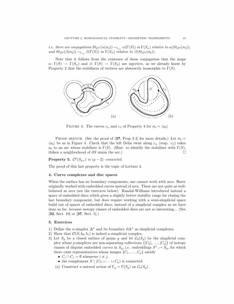
Property 4. Let S = Sg,r and let Sα ∼= Sg+1,r−1 and Sβ ∼= Sg,r+1 denote Sunion a strip glued via α and β respectively as in Figure 3. Then for any vertexσ0 of Oi(S), there are curves cα, cβ (given in Figure 4) in Sα and Sβ such thatconjugation by Dehn twists tcα and tcβ along these curves fits into commutativediagrams
StO2(σ0) _
// StO1(α(σ0)) _
tcα
wwp p p p p pStO1(σ0) _
// StO2(β(σ0)) _
tcβ
wwp p p p p p
Γ(S) α // Γ(Sα) Γ(S)β
// Γ(Sβ)
LECTURE 2. HOMOLOGICAL STABILITY: GEOMETRIC INGREDIENTS 15
i.e. there are conjugations StO1(α(σ0)) ∼tcα α(Γ(S)) in Γ(Sα) relative to α(StO2(σ0)),and StO2(β(σ0)) ∼tcβ β(Γ(S)) in Γ(Sβ) relative to β(StO1(σ0)).
Note that it follows from the existence of these conjugation that the mapsα : Γ(S) → Γ(Sα) and β : Γ(S) → Γ(Sβ) are injective, as we already know byProperty 2 that the stabilizers of vertices are abstractly isomorphic to Γ(S).
αβ
a0
a0
cα
cβ
(a) (b)
Figure 4. The curves cα and cβ of Property 4 for σ0 = 〈a0〉
Proof sketch. (See the proof of [37, Prop 2.4] for more details.) Let σ0 =〈a0〉 be as in Figure 4. Check that the left Dehn twist along cα (resp. cβ) takesa0 to an arc whose stabilizer is Γ(S). (Hint: to identify the stabilizer with Γ(S),thiken a neighborhood of ∂S union the arc.)
Property 5. Oi(Sg,r) is (g − 2)–connected.
The proof of this last property is the topic of Lecture 4.
4. Curve complexes and disc spaces
When the surface has no boundary components, one cannot work with arcs. Hareroriginally worked with embedded curves instead of arcs. These are not quite as well-behaved as arcs (see the exercices below). Randal-Williams introduced instead aspace of embedded discs which gives a slightly better stability range for closing thelast boundary component, but does require working with a semi-simplicial spacebuild out of spaces of embedded discs, instead of a simplicial complex as we havedone so far, because isotopy classes of embedded discs are not so interesting... (See[32, Sect. 10] or [37, Sect. 5].)
5. Exercices
1) Define the n-simplex ∆n and its boundary ∂∆n as simplicial complexes.2) Show that O(S, b0, b1) is indeed a simplicial complex.3) Let Sg be a closed surface of genus g and let C0(Sg) be the simplicial com-
plex whose p-simplices are non-separating collections [C0], . . . , [Cp] of isotopyclasses of disjoint embedded curves in Sg, i.e. embeddings S1 → Sg, for whichthere exist representatives whose images C1, . . . , Cp satisfy• Ci ∩ Cj = ∅ whenever i 6= j,• the complement S \ (C0 ∪ · · · ∪ Cp) is connected.
(a) Construct a natural action of Γg = Γ(Sg) on C0(Sg).
16 NATHALIE WAHL, MUMFORD CONJECTURE, MADSEN-WEISS AND STABILITY
(b) Show that this action is transitive on p-simplices for each p ≥ 0. (Hint:as in the proof of Property 1 above, first use the classification of surfacesto prove that the complement of two such collections of p + 1 circles arediffeomorphic.)
(c) Construct a map from Γg−1,2 to the stabilizer of a vertex of C0(Sg) andprove that it is surjective using the isotopy extension theorem as in theproof of Property 2. Is it injective?
4) Complete the proof of Property 4.5) Let M and N be smooth manifolds. Denote by C0(M,N) the set of continuous
maps from M to N , and denote by Emb0(M,N) ⊂ C0(M,N) the subset con-sisting of topological embeddings. Inductively, for k > 0 denote by Ck(M,N) ⊂Ck−1(M,N) the subset consisting of differentiable maps f : M → N for whichthe induced map on tangent spaces Tf is in Ck−1(TM, TN). We topologizethe set Ck(M,N) inductively: we use the compact-open topology on C0(M,N),and we note that D : Ck(M,N) → Ck−1(TM, TN) is an inclusion, so we giveCk(M,N) the subspace topology. We let C∞(M,N) denote the inverse limit ofthe Ck(M,N).
Denote by Embk(M,N) ⊂ Ck(M,N) the subspace consisting of topologicalembeddings e for which Te is in Embk−1(TM, TN), and write the inverse limitas Emb(M,N). Denote by Diff(M) ⊂ Emb(M,M) the subspace consisting ofthose invertible maps φ for which φ−1 ∈ Diff(M).(a) Prove that a sequence of maps fn ∈ C1(R,R) converges if and only if the
sequences fn ∈ C0(R,R) and f ′n ∈ C0(R,R) converge.(b) Prove that this inclusion Embk([0, 1],R) ⊂ Ck([0, 1],R) is open when k = 1
but not when k = 0.(c) (difficult) In this exercise we will prove that if N is a compact submanifold
of M , then the restriction map
j : Emb(M,Rn) −→ Emb(N,Rn)
is locally trivial fibration (i.e. a fibre bundle with structure group the fullhomeomorphism group of the fibre). This was first proved by Palais andCerf, but we follow Lima [22].
(i) Given a f ∈ Emb(N,Rn), show there is a neighbourhood U of f anda map ξ : U → Diff(Rn) such that ξ(g) f = g. [Hint: note thatDiff(Rn) is an open subset of C∞(Rn,Rn).]
(ii) Hence construct a trivialisation of j over U .
Remark 2.3. Note that this implies it is in particular a Serre fibration,and hence the existence of a long exact sequence on homotopy groups
· · · → πn+1F → πn Emb(M,Rn)→ πn Emb(N,Rn)→ πnF →· · · ,where F is the fiber of the restriction map over some base point f ∈Emb(N,Rn).
LECTURE 3
Homological stability: the spectral sequenceargument
In this lecture, we present a spectral sequence argument (the one used byRandal-Williams in [32]) which allows to prove homological stability for the map-ping class groups of surfaces in the range stated in Lecture 1. We will consider thetwo spectral sequences associated to a double chain complex build from a pair ofgroups acting on a pair of spaces. We will then use all the geometric propertiespresented in Lecture 2 to analyze these spectral sequences.
1. Double complexes associated to actions on simplicial complexes
ToX a simplicial complex, one can associate a chain complex (C∗, ∂) (its augmentedcellular complex) which computes the reduce homology of its realization |X|. It has
• Cp(X) = ZXp, the free module on the set of p-simplices• C−1(X) = Z
with boundary maps coming from the face maps and the augmentation.We are interested here in simplicial complexes X admiring a simplicial G–action
for some group G. For such, one can construct a double complex
E∗G⊗G C∗(X)
where · · · → EqG → · · · → E0G → Z → 0 is a free resolution of Z over ZG. Thisis the basic double complex commonly used to prove homological stability results.We will use here a relative version of it, which we construct now.
Suppose Y in addition is a simplicial complex with a simplicial H–action andf : X → Y a simplicial map equivariant with respect to a map G → H. Then weget a map of double complexes
F : E∗G⊗G C∗(X) −→ E∗H ⊗H C∗(Y )
(The two examples of interest to us are the maps α : O2 → O1 and β : O1 → O2
of Lecture 2 and their companion maps on the mapping class groups.) We will usethe double complex
Cp,q = (Eq−1G⊗G Cp(X))⊕ (EqH ⊗H Cp(Y ))with horizontal differential (a⊗ b, a′ ⊗ b′) 7→ (a⊗ ∂b, a′ ⊗ ∂b′)and vertical differential (a⊗ b, a′ ⊗ b′) 7→ (da⊗ b, da′ ⊗ b′ + F (a⊗ b))(i.e. for each p we take the mapping cone of F in the q–direction).
The horizontal and vertical filtrations of such a double complex give two spec-tral sequences, both converging to the homology of the total complex. We nowanalyze these two spectral sequences.
17
18 NATHALIE WAHL, MUMFORD CONJECTURE, MADSEN-WEISS AND STABILITY
2. The spectral sequence associated to the horizontal filtration
As Eq−1G and EqH are free G– (resp. H–)modules and the horizontal differentialis that of C(X) and C(Y ), taking first the homology in the p–direction computescopies of the reduced homology of X plus that of Y .
In particular, if X is (c − 1)–connected and Y is c–connected, the E1–termof the horizontal spectral sequence, which is the homology of Cp,q with respect tothe horizontal differential, is 0 in the range p + q ≤ c (noting that Cp(X) onlycontributes to Cp,q when q > 0).
It follows that the other spectral sequence, obtained using the vertical filtrationinstead, also converges to 0 in the range p+ q ≤ c.
3. The spectral sequence associated to the vertical filtration
For each p, the module Cp(X) = ZXp is a G-module, which decomposes as a sumof modules corresponding to the orbits of the G-action on Xp. (We define hereX−1 = ∗ with the trivial action.) Given an orbit o ∈ O(Xp), the set of orbits ofXp, we let Stab(o) ≤ G denote the stabilizer subgroup of some chosen simplex σp inthe orbit o. Assuming that the stabilizer of a simplex fixes the simplex pointwise,we can rewrite the G-module Cp(X) as
Cp(X) ∼=⊕
o∈O(Xp)
G⊗Stab(o) Z
The chain complex E∗(G)⊗G Cp(X), where p is now fixed, computes the homologyof G with coefficients in that module. (This is the definition of the homology of agroup with twisted coefficients.)
We will use a relative version (left as an exercise) of the following well-knownlemma (see e.g. [5, III 6.2]):
Lemma 3.1 (Shapiro’s lemma). Let H < G be groups and M be an H–module,with G⊗H M the induced G-module. Then
H∗(G,G⊗H M) ∼= H∗(H,M)
Hence for any G–simplicial complex X as above, we have, for each p, that
H∗(E∗G⊗ Cp(X)) ∼=⊕
o∈O(Xp)
H∗(Stab(o)).
The E1–term of the vertical spectral sequence is the homology of the doublecomplex Cp,q = (Eq−1G⊗G Cp(X))⊕ (EqH ⊗H Cp(Y )) with respect to the verticaldifferential. This is the relative homology group
E1p,q = Hq
(E∗H ⊗H Cp(Y ), E∗G⊗G Cp(X)
)as the columns of Cp,q are the mapping cones of the map F (with p fixed).
Now if the actions of G and H are transitive on X and Y (which is the casewe are interested in), a relative version of Shapiro’s lemma identifies the E1–termof the vertical spectral sequence with
E1p,q = Hq(StabY (σp),StabX(σp))
LECTURE 3. HOMOLOGICAL STABILITY: THE SPECTRAL SEQUENCE ARGUMENT 19
where StabX(σp) and StabY (σp) are the stabilizers in X and Y of some chosen p–simplex σp of X and its image in Y . Note that this formulation in the case p = −1gives
E1−1,q = Hq(H,G)
4. The proof of stability for surfaces with boundaries
Recall from the previous lecture the maps
αg : Γ(Sg,r+1)→ Γ(Sg+1,r) and βg : Γ(Sg,r)→ Γ(Sg,r+1).
Denote by H(αg) the relative homology group H(Γg+1,r,Γg,r+1; Z) correspond-ing to the map αg, and H(βg) the relative homology group H(Γg,r+1,Γg,r; Z) corre-sponding to βg. (The number of boundaries r here will not play a role here.) Harer’simproved stability theorem (Theorem 1.3) can be restated as follows [exercise]:
Theorem 3.2. (1) Hi(αg) = 0 for i ≤ 2g+13 and (2) Hi(βg) = 0 for i ≤ 2g
3 .
The proof of this theorem uses the spectral sequences just described in thecase of the maps α and β of Lecture 2. The argument will need Properties 1–5 ofLecture 2.
Proof. We prove the theorem by induction on g. To start the induction, notethat statements (1) for genus 0 and (2) for genus 0,1 are trivially true as they arejust concerned with H0. Let (1g) and (2g) denote the truth of (1) and (2) in thetheorem for genus g. The induction will go in two steps:
Step 1: For g ≥ 1, (2≤g) implies (1g).Step 2: For g ≥ 2, (1<g) and (2g−1) imply (2g).
Step 1: We consider the spectral sequence described above for the actions ofG = Γg,r+1 on X = O2(Sg,r+1) and of H = Γg+1,r on Y = O1(Sg+1,r) withthe homomorphism φ : G → H and the map f : X → Y both induced by themap α : Sg,r+1 → Sg+1,r of Figure 3. As the action is transitive in both cases(Property 1), we get, as explained above, that the vertical spectral sequence hasthe form E1
p,q = Hq(StabY (α(σp)),StabX(σp)), with σp a chosen p-simplex of Xand α(σp) its image in Y . That is, when p = −1, we have
E1−1,q = Hq(Γg+1,r,Γg,r+1) = Hq(αg)
which are the groups we are interested in. By Properties 2 and 3, the other groupsare identified with
E1p,q = Hq(βg−p) for p ≥ 0.
Hence we will be able to apply induction to these terms of the spectral sequence.We want to deduce that E1
−1,q = 0 for q ≤ 2g+13 . This will follow from the following
three claims:Claim 1: E∞−1,q = 0 for q ≤ 2g+1
3 .Claim 2: The E1–term is as in Figure 1, i.e. there are no possible sources ofdifferentials to kill classes in E1
−1,q with q ≤ 2g+13 , except possibly for d1 : E1
0,q →E1−1,q when q = 2g+1
3 (i.e. when the fraction is an integer).Claim 3: The map d1 : E1
0,q → E1−1,q is the 0-map.
Claims 1 and 2 imply immediately that E1−1,q = 0 for q < 2g+1
3 as “it must dieby E∞” (Claim 1) and “nobody can kill it” (Claim 2). Claim 3 gives that this also
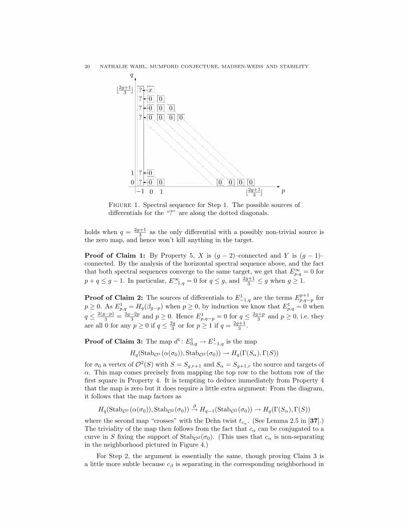
20 NATHALIE WAHL, MUMFORD CONJECTURE, MADSEN-WEISS AND STABILITY
b2g+13 c
q
10
b2g+13 c p10−1
00
0 0 0 0 0
0 0 0 00 0 00 0x?
???
??
Figure 1. Spectral sequence for Step 1. The possible sources ofdifferentials for the “?” are along the dotted diagonals.
holds when q = 2g+13 as the only differential with a possibly non-trivial source is
the zero map, and hence won’t kill anything in the target.
Proof of Claim 1: By Property 5, X is (g − 2)–connected and Y is (g − 1)–connected. By the analysis of the horizontal spectral sequence above, and the factthat both spectral sequences converge to the same target, we get that E∞p,q = 0 forp+ q ≤ g − 1. In particular, E∞−1,q = 0 for q ≤ g, and 2g+1
3 ≤ g when g ≥ 1.
Proof of Claim 2: The sources of differentials to E1−1,q are the terms Ep+1
p,q−p forp ≥ 0. As E1
p,q = Hq(βg−p) when p ≥ 0, by induction we know that E1p,q = 0 when
q ≤ 2(g−p)3 = 2g−2p
3 and p ≥ 0. Hence E1p,q−p = 0 for q ≤ 2g+p
3 and p ≥ 0, i.e. theyare all 0 for any p ≥ 0 if q ≤ 2g
3 or for p ≥ 1 if q = 2g+13 .
Proof of Claim 3: The map d1 : E10,q → E1
−1,q is the map
Hq(StabO1(α(σ0)),StabO2(σ0))→ Hq(Γ(Sα),Γ(S))
for σ0 a vertex of O2(S) with S = Sg,r+1 and Sα = Sg+1,r the source and targets ofα. This map comes precisely from mapping the top row to the bottom row of thefirst square in Property 4. It is tempting to deduce immediately from Property 4that the map is zero but it does require a little extra argument: From the diagram,it follows that the map factors as
Hq(StabO1(α(σ0)),StabO2(σ0)) ∂→ Hq−1(StabO2(σ0))→ Hq(Γ(Sα),Γ(S))
where the second map “crosses” with the Dehn twist tcα . (See Lemma 2.5 in [37].)The triviality of the map then follows from the fact that cα can be conjugated to acurve in S fixing the support of StabO2(σ0). (This uses that cα is non-separatingin the neighborhood pictured in Figure 4.)
For Step 2, the argument is essentially the same, though proving Claim 3 isa little more subtle because cβ is separating in the corresponding neighborhood in
LECTURE 3. HOMOLOGICAL STABILITY: THE SPECTRAL SEQUENCE ARGUMENT 21
Figure 4. It is necessary to use induction an extra time here to finish the argument.(See the proof of [37, Thm 3.1 (2)] for the details.)
5. Closing the boundaries
To prove that the map δ : Γg,1 → Γg,0 also induces a homology isomorphism ina range, one uses a similar spectral sequence for the action of the mapping classgroups on the disc semi-simplicial space of [32] (or the curve complex as in [16])and compare the spectral sequence for each case (a comparison argument goingback to [20]). See [37, Sect 5] for details.
6. Exercises
1) State and prove the relative version of Shapiro’s lemma needed in the analysisof the vertical spectral sequence above.
2) Show that Theorem 3.2 implies the first part of Theorem 1.3 of Lecture 1.3) This exercise sets up a way of approaching the proof of homological stability for
the symmetric groups.(a) Let ∆n denote the n–simplex. It can be thought of as a simplicial complex
with n+1 vertices 0, . . . , n, the set of p-simplices being the set of subsetsof 0, . . . , n of cardinality p+1. Consider the action of the symmetric groupΣn+1 on ∆n induced by permuting the vertices. Show that the action istransitive on the set of p-simplices for each p. What is the stabilizer of avertex? of a p-simplex in general? (Note that the stabilizer of a simplexis the subgroup of symmetries that map the simplex to itself, as a set ofvertices.)
(b) Replace ∆n in the above exercise by the semi-simplicial set (=simplicialset without degeneracies) Xn+1 whose p-simplices are injective maps σ :0, 1, . . . , p → 0, . . . , n. Is the action of Σn+1 still transitive on the setof p-simplices for any p? What is the stabilizer of a p-simplex in this case?
(c) For a semi-simplicial set Y = Y∗, let ||Y || =∐p≥0 ∆p × Yp/ ∼ denote
its realization, where the equivalence relation ∼ is induced by the facerelations. For X1, X2, X3 as in (b), show that ||X1|| = ∗, ||X2|| ∼= S1 andthat ||X3|| is simply-connected.
(d) Consider the cellular chain complex C∗(Xn+1) with its induced actionof Σn+1. Pick a free resolution E∗Σn+1 of Z considered as a Z[Σn+1]-module with a trivial action of Σn+1. Now consider the double complexCp,q = Cp(Xn+1) ⊗Σn+1 EqΣn+1. Write down the E1-terms of the associ-ated spectral sequences in both filtrations.
Remark 3.3. Given thatXn is (n−2)-connected (see [34, Prop 3.2] or [21]), onecan use the above spectral sequences to prove Nakaoka’s stability theorem: themap Hq(Σn)→ Hq(Σn+1) induced by the inclusion of groups is an isomorphismfor q ≤ n/2.
4) The action of the mapping class group Γg on the Teichmuller space Tg satisfiesthat the stabilizers of points are finite (most often trivial) groups (see e.g. [9,12.1]). Let C∗(Tg,Q) denote the singular chain complex of Tg with rationalcoefficients. The action of the mapping class group gives rise, as above, to adouble complex C∗(Tg,Q) ⊗Γg E∗Γg, with E∗Γg now a free resolution of Q asa trivial Q[Γg]-module. Using the spectral sequences associated to the double
22 NATHALIE WAHL, MUMFORD CONJECTURE, MADSEN-WEISS AND STABILITY
complex, show that the coarse moduli space Tg/Γg is rationally a classifyingspace for Γg, i.e. that H∗(Tg/Γg,Q) ∼= H∗(BΓg,Q).
LECTURE 4
Homological stability: the connectivity argument
In this lecture, we give a sketch proof of the last ingredient of the proof ofhomological stability for mapping class groups of surfaces with boundaries, namelythe fact that the complex O(S; b0, b1) of Lecture 2 is (g − 2)-connected for anysurface S of genus g. To close the surfaces, an analogous statement is needed forthe disc space or curve complex, which is not presented here. We refer instead [32],[37], or [20] for that case.
1. Strategy for computing the connectivity of the ordered arc complex
We will prove that O(S; b0, b1) is highly connected by working our way through thefollowing sequence of smaller and smaller simplicial complexes:
A(S,∆)i1← B(S,∆0,∆1)
i2← B0(S,∆0,∆1)i3← O(S, b0, b1)
where ∆,∆0,∆1 are sets of points in ∂S andA(S,∆) is the simplicial complex whose vertices are isotopy
classes of all non-trivial arcs in S with boundary in ∆. Ap–simplex of A(S,∆) is a collection of p+ 1 distinct isotopyclasses of arcs 〈a0, . . . , ap〉 representable by arcs with disjointinteriors.
B(S,∆0,∆1) ⊂ A(S,∆0 ∪∆1) is the subcomplex of arcs havingeach one boundary point in ∆0 and one in ∆1.
B0(S,∆0,∆1) ⊂ B(S,∆0,∆1) is the subcomplex of non-separatingcollections.
O(S, b0, b1) ⊂ B0(S, b0, b1 is the ordered subcomplex (de-fined in Lecture 2, Section 3).
The largest complex A(S,∆) is contractible in most cases, and one slowly loosesconnectivity as one goes down to smaller and smaller subcomplexes.
The connectivity arguments used are of three types:(1) direct calculation showing contractibility,(2) exhibition of a complex as a suspension (or wedge of such) of a “previous”
complex,(3) inductive deduction from the connectivity of a larger complex.The argument for the connectivity of A(S,∆) is a mix of type (1) and (2), thededuction along i1 in the sequence is the most intricate argument and is a mixof the three types of arguments, while deduction along i2 and i3 are purely (andsimpler) type (3) arguments.
We do here, to exemplify, a type (1) and a type (3) argument and refer to [37]for the complete proofs.
23
24 NATHALIE WAHL, MUMFORD CONJECTURE, MADSEN-WEISS AND STABILITY
2. Contractibility of the full arc complex
Theorem 4.1. [16, Thm 1.5] Suppose S is not a disc or a cylinder with ∆ includedin a single boundary of S. Then A(S,∆) is contractible.
Sketch of proof of the main case, following Hatcher [17]. (See alsothe proof of [37, Thm 4.1] for a complete proof.) We will prove the theorem un-der the extra assumption that S has at most one point of ∆ in each boundarycomponent. Reducing to that case requires an extra (type (2)) argument.
Non-emptiness: Clear if |∆| > 1 by choosing any arc in the surface between twodistinct points of ∆—such an arc is always non-trivial as the points lie on differentboundary components. For |∆| = 1, we have assumed that S is not a disc or acylinder, i.e. S has non-zero genus or at least three boundary components. In bothcases, there are non-trivial arcs.
In a simplicial complexX, the star of a simplex σ is the union of all the simplicesτ of X such that σ ∪ τ is again a simplex of X. This is a contractible subcomplex.
Contraction: As A(S,∆) is non-empty, we can choose an arc a ∈ A(S,∆). Wewill contract the complex to the star of a.
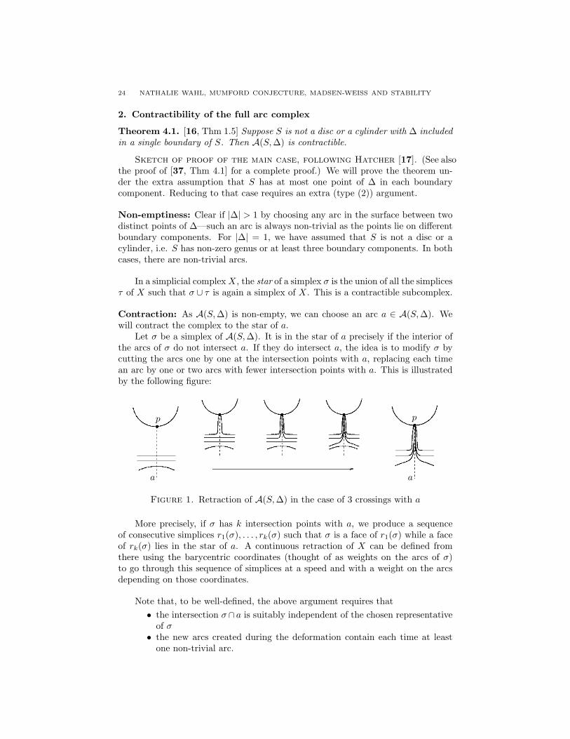
Let σ be a simplex of A(S,∆). It is in the star of a precisely if the interior ofthe arcs of σ do not intersect a. If they do intersect a, the idea is to modify σ bycutting the arcs one by one at the intersection points with a, replacing each timean arc by one or two arcs with fewer intersection points with a. This is illustratedby the following figure:
p
a
p
a
Figure 1. Retraction of A(S,∆) in the case of 3 crossings with a
More precisely, if σ has k intersection points with a, we produce a sequenceof consecutive simplices r1(σ), . . . , rk(σ) such that σ is a face of r1(σ) while a faceof rk(σ) lies in the star of a. A continuous retraction of X can be defined fromthere using the barycentric coordinates (thought of as weights on the arcs of σ)to go through this sequence of simplices at a speed and with a weight on the arcsdepending on those coordinates.
Note that, to be well-defined, the above argument requires that• the intersection σ∩ a is suitably independent of the chosen representative
of σ• the new arcs created during the deformation contain each time at least
one non-trivial arc.
LECTURE 4. HOMOLOGICAL STABILITY: THE CONNECTIVITY ARGUMENT 25
The first issue is addressed by choosing representative with minimal intersectionwith a, and the second is addressed by the additional assumption we worked with,namely that there is at most one point of ∆ in each boundary component.
3. Deducing connectivity of smaller complexes
The connectivity of the subcomplex B(S,∆0,∆1) of arcs between two subsets ∆0
and ∆1 of ∆ is deduced from that of A(S,∆) by a long argument... To be ableto state the connectivity bound, we need a couple of definitions: Disjoint sets∆0,∆1 ⊂ ∂S define a decomposition of ∂S into vertices (the points of ∆0 ∪ ∆1),edges between the vertices, and circles without vertices. We say that an edge ispure if both its endpoints are in the same set, ∆0 or ∆1. We say that an edge isimpure otherwise. Note that the number of impure edges is always even.
Theorem 4.2. [16, Thm 1.6] The complex B(S,∆0,∆1) is (4g+r+r′+ l+m−6)–connected, where g is the genus of S, r its number of boundary components, r′ thenumber of components of ∂S containing points of ∆0 ∪∆1, l is half the number ofimpure edges and m is the number of pure edges.
See [37, Thm 4.3] for a detailed proof.
We will now use the connectivity of B(S,∆0,∆1) to deduce that of the sub-complex B0(S,∆0,∆1) of non-separating simplices.
The join X ∗ Y of two simplicial complexes X and Y is the simplicial complexwith vertices X0tY0 and a (p+q+1)–simplex σX ∗σY = 〈x0, . . . , xp, y0, . . . , yq〉 foreach p–simplex σX = 〈x0, . . . , xp〉 of X and q–simplex σY = 〈y0, . . . , yq〉 of Y . Notethat |X ∗ Y | = |X| ∗ |Y |, i.e. the realization of the join complex is the (topological)join of the realization of the two complexes. This follows from the fact that it istrue for each pair of simplices.
Recall that a space (or simplicial complex) X is called n–connected if πi(X) = 0for all i ≤ n For n = −1, we use the convention that (−1)–connected means non-empty. (For n ≤ −2, n–connected is a void property.)
The following proposition tells us how to compute the connectivity of a join interms of the connectivity of the pieces.
Proposition 4.3. [27, Lem 2.3] Consider the join X = X1∗· · ·∗Xk of k non-emptyspaces. If each Xi is ni–connected, then X is
((∑ki=1(ni + 2)
)− 2)–connected.
Theorem 4.4. [16, Thm 1.4] If ∆0,∆1 are two disjoint non-empty sets of pointsin ∂S, then the complex B0(S,∆0,∆1) is (2g + r′ − 3)–connected, for g and r′ asabove.
Proof. We prove the theorem by induction on the lexicographically orderedtriple (g, r, q), where r ≥ r′ is the number of components of ∂S and q = |∆0∪∆1| ≥2. To start the induction, note that the theorem is true when g = 0 and r′ ≤ 2 forany r ≥ r′ and any q, and more generally that the complex is non-empty wheneverr′ ≥ 2 or g ≥ 1.
So fix (S,∆0,∆1) satisfying (g, r, q) ≥ (0, 3, 2). Then 2g+ r′−3 ≤ 4g+ r+ r′+l+m− 6. Indeed, r ≥ 1 and l+m ≥ 1. Moreover we assumed that either r ≥ 3 org ≥ 1.
Let k ≤ 2g + r′ − 3 and consider a map f : Sk → B0(S,∆0,∆1), which we mayassume to be simplicial for some PL triangulation of Sk (see [37, Sect 6]). This
26 NATHALIE WAHL, MUMFORD CONJECTURE, MADSEN-WEISS AND STABILITY
map can be extended to a simplicial map f : Dk+1 → B(S,∆0,∆1) by Theorem 4.2and the above calculation, for a PL triangulation of Dk+1 extending that of Sk. Wecall a simplex σ of Dk+1 regular bad if f(σ) = 〈a0, . . . , ap〉 and each aj separatesS\(a0 ∪ . . . aj · · · ∪ ap). Let σ be a regular bad simplex of maximal dimension p.Write S\f(σ) = X1 t · · · t Xc with each Xi connected. By maximality of σ, frestricts to a map
Link(σ) −→ Jσ = B0(X1,∆10,∆
11) ∗ · · · ∗ B0(Xc,∆c
0,∆c1)
where each ∆iε is inherited from ∆ε and is non-empty as the arcs of f(σ) are impure.
Each Xi has (gi, ri, qi) < (g, r, q), so by induction B0(Xi,∆i0,∆
i1) is (2gi + r′i − 3)–
connected. The Euler characteristic gives∑i(2 − 2gi − ri) = 2 − 2g − r + p′ + 1,
where p′+1 ≤ p+1 is the number of arcs in f(σ). We also have∑i(ri−r′i) = r−r′,
so∑
(2gi + r′i) = 2g+ r′ − p′ + 2c− 3. Now Jσ is (∑i(2gi + r′i − 1)− 2)–connected
(using Proposition 4.3), that is (2g+r′−p′+c−5)–connected. As c ≥ 2 and p′ ≤ p,we can extend the restriction of f to Link(σ) ' Sk−p to a map F : K → Jσ with Ka (k− p+ 1)–disc with boundary the link of σ. We modify f on the interior of thestar of σ using f ∗ F on ∂σ ∗K ' Star(σ). If a simplex α ∗ β in ∂σ ∗K is regularbad, β must be trivial since β does not separate S\f(α), so that α ∗ β = α is aface of σ. We have thus reduced the number of regular bad simplices of maximaldimension and the result follows by induction.
From there, one can prove by a similar type of argument that the orderedsubcomplex is also highly connected:
Theorem 4.5 (Property 5). O(S, b0, b1) is (g − 2)–connected.
See [37, Thm 4.9] for a detailed proof.
4. Exercises
1) The complex C0(S) of the exercises of Lecture 2 is a subcomplex of the complexC(S) with vertices all isotopy classes of non-trivial circles in S and p-simplicesall disjointly embeddable collections of p+ 1 distinct isotopy classes. Assumingthat C(S) is (2g+r−4)–connected if S has genus g and r boundary components,show that C0(S) is (g − 2)–connected.
Bibliography
[1] Arnol’d, V. I. Certain topological invariants of algebraic functions. (Russian) Trudy
Moskov. Mat. Obsc. 21 1970 27–46. English transl. in Trans. Moscow Math. Soc.21 (1970), 30–52.
[2] Barratt, M. G.; Eccles, Peter J. Γ+-structures. I. A free group functor for stable
homotopy theory. Topology 13 (1974), 2545.[3] Boardman, J. M.; Vogt, R. M. Homotopy invariant algebraic structures on topo-
logical spaces. Lecture Notes in Mathematics, Vol. 347.
[4] Boldsen, Søren K. Improved homological stability for the mapping class group withintegral or twisted coefficients. To appear in Math. Z. (2010).
[5] Brown, Kenneth S. Cohomology of groups. Corrected reprint of the 1982 original.Graduate Texts in Mathematics, 87. Springer-Verlag, New York, 1994.
[6] Cerf, Jean. Topologie de certains espaces de plongements. (French) Bull. Soc. Math.
France 89 1961 227-380.[7] Cohen, Frederick R.; Lada, Thomas J.; May, J. Peter. The homology of iterated
loop spaces. Lecture Notes in Mathematics, Vol. 533. Springer-Verlag, Berlin-New
York, 1976.[8] Earle, Clifford J.; Eells, James. A fibre bundle description of Teichmuller theory.
J. Differential Geometry 3 1969 19–43.
[9] Farb, Benson; Margalit, Dan. A primer on mapping class groups. To be publishedby Princeton University Press. (Available at http://www.math.utah.edu/ mar-
galit/primer/)
[10] Galatius, Søren. Stable homology of automorphism groups of free groups. Ann. ofMath. (2) 173 (2011), no. 2, 705-768.
[11] Galatius, Søren. Lectures on the Madsen-Weiss theorem. [ Lectures, same vol-ume ] .
[12] Soren Galatius, Oscar Randal-Williams. Monoids of moduli spaces of manifolds.
Geom. Topol. 14 (2010), no. 3, 1243-1302.[13] Charney, Ruth M. Homology stability for GLn of a Dedekind domain. Invent.
Math. 56 (1980), no. 1, 117.
[14] Galatius, Søren; Tillmann, Ulrike; Madsen, Ib; Weiss, Michael. The homotopy typeof the cobordism category. Acta Math. 202 (2009), no. 2, 195–239.
[15] Gramain, Andre. Le type d’homotopie du groupe des diffeomorphismes d’une sur-
face compacte. (French) Ann. Sci. Ecole Norm. Sup. (4) 6 (1973), 53–66.
[16] Harer, John L. Stability of the homology of the mapping class groups of orientable
surfaces. Ann. of Math. (2) 121 (1985), no. 2, 215–249.[17] Hatcher, Allen. On triangulations of surfaces. Topology Appl.
40 (1991), no. 2, 189–194. (Updated version available athttp://www.math.cornell.edu/ hatcher/Papers/TriangSurf.pdf.)
[18] Hatcher Allen. In preparation.
(See http://www.math.cornell.edu/ hatcher/Papers/luminytalk.pdf)[19] Ivanov, Nikolai V. Stabilization of the homology of Teichmuller modular groups.
(Russian) Algebra i Analiz 1 (1989), no. 3, 110–126; translation in Leningrad Math.J. 1 (1990), no. 3, 675–691.
[20] Ivanov, Nikolai V. On the homology stability for Teichmuller modular groups:closed surfaces and twisted coefficients. Mappping Class Groups and Moduli Spaces
of Riemann Surfaces, Contemporary Mathematics, V. 150, American MathematicalSociety, 1993, 149-194.
27
28 NATHALIE WAHL, MUMFORD CONJECTURE, MADSEN-WEISS AND STABILITY
[21] Kerz, Moritz. The complex of words and Nakaoka stability. Homology Homotopy
Appl. 7 (2005), no. 1, 77–85.
[22] Lima, Elon L. On the local triviality of the restriction map for embeddings. Com-ment. Math. Helv. 38 (1964), 163–164.
[23] Madsen, Ib; Weiss, Michael. The stable moduli space of Riemann surfaces: Mum-
ford’s conjecture. Ann. of Math. (2) 165 (2007), no. 3, 843–941.[24] May, J. P. The geometry of iterated loop spaces. Lectures Notes in Mathematics,
Vol. 271. Springer-Verlag, Berlin-New York, 1972.
[25] McDuff, D.; Segal, G. Homology fibrations and the “group-completion” theorem.Invent. Math. 31 (1975/76), no. 3, 279284.
[26] Mumford, David. Towards an enumerative geometry of the moduli space of curves.
Arithmetic and geometry, Vol. II, Progr. Math. 36 (1983), 271–328.[27] Milnor, John. Construction of universal bundles. II. Ann. of Math. (2) 63 (1956),
430–436.[28] Morita, Shigeyuki. Geometry of characteristic classes. Translated from the 1999
Japanese original. Translations of Mathematical Monographs, 199. Iwanami Series
in Modern Mathematics. American Mathematical Society, Providence, RI, 2001.[29] Nakaoka, Minoru. Decomposition theorem for homology groups of symmetric
groups. Ann. of Math. (2) 71 (1960), 16–42.
[30] Palais, Richard S. Local triviality of the restriction map for embeddings. Comment.Math. Helv. 34 1960 305-312.
[31] Priddy, Stewart B. On Ω∞S∞ and the infinite symmetric group. Algebraic topol-
ogy (Proc. Sympos. Pure Math., Vol. XXII, Univ. Wisconsin, Madison, Wis., 1970),pp. 217220. Amer. Math. Soc., Providence, R.I., 1971.
[32] Randal-Williams, Oscar. Resolutions of moduli spaces and homological stability.
Preprint, 2009 (arXiv:0909.4278).[33] Randal-Williams, Oscar. Homology of the moduli spaces and mapping class groups
of framed and Pin surfaces. Preprint (arXiv:1001.5366).[34] Randal-Williams, Oscar. Homological stability for unordered configuration spaces.
Preprint, 2011 (arXiv:1105.5257).
[35] Segal, Graeme Configuration-spaces and iterated loop-spaces. Invent. Math. 21(1973), 213221.
[36] Wahl, Nathalie. Homological stability for the mapping class groups of non-
orientable surfaces. Invent. Math. 171 (2008), no. 2, 389–424.[37] Wahl, Nathalie. Homological stability for mapping class groups of surfaces. Preprint
(2011). To appear in the Handbook of Moduli.


![THE MUMFORD CONJECTURE [after Madsen and Weiss] …andyp/teaching/2011FallMath541/PowellSurvey.pdf · THE MUMFORD CONJECTURE [after Madsen and Weiss] by Geoffrey POWELL 1. INTRODUCTION](https://img.pdfslide.net/doc/110x75/5e7a09cb7334ee1c0922902b/the-mumford-conjecture-after-madsen-and-weiss-andypteaching2011fallmath541.jpg)

![Shimura Varieties and the Mumford–Tate conjecture, part I · 2018. 11. 24. · arXiv:math/0109094v1 [math.NT] 14 Sep 2001 Shimura Varieties and the Mumford–Tate conjecture, part](https://img.pdfslide.net/doc/110x75/606be3d5bd366d74a156014c/shimura-varieties-and-the-mumfordatate-conjecture-part-i-2018-11-24-arxivmath0109094v1.jpg)