Embed Size (px)
Citation preview

WAKE WORD DETECTION AND ITS APPLICATIONS
by
Yiming Wang
A dissertation submitted to The Johns Hopkins University in conformity with the
requirements for the degree of Doctor of Philosophy
Baltimore, Maryland
July 2021
© 2021 Yiming Wang
All rights reserved

Abstract
Always-on spoken language interfaces, e.g. personal digital assistants, rely on a wake
word to start processing spoken input. Novel methods are proposed to train a wake word
detection system from partially labeled training data, and to use it in on-line applications.
In the system, the prerequisite of frame-level alignment is removed, permitting the use
of un-transcribed training examples that are annotated only for the presence/absence of the
wake word. Also, an FST-based decoder is presented to perform online detection. The suite
of methods greatly improve the wake word detection performance across several datasets.
A novel neural network for acoustic modeling in wake word detection is also inves-
tigated. Specifically, the performance of several variants of chunk-wise streaming Trans-
formers tailored for wake word detection is explored, including looking-ahead to the next
chunk, gradient stopping, different positional embedding methods and adding same-layer
dependency between chunks. Experiments demonstrate that the proposed Transformer
model outperforms the baseline convolutional network significantly with a comparable
model size, while still maintaining linear complexity w.r.t. the input length.
For the application of the detected wake word in ASR, the problem of improving speech
ii

recognition with the help of the detected wake word is investigated. Voice-controlled
house-hold devices face the difficulty of performing speech recognition of device-directed
speech in the presence of interfering background speech. Two end-to-end models are pro-
posed to tackle this problem with information extracted from the anchored segment. The
anchored segment refers to the wake word segment of the audio stream, which contains
valuable speaker information that can be used to suppress interfering speech and back-
ground noise. A multi-task learning setup is also explored where the ideal mask, obtained
from a data synthesis procedure, is used to guide the model training. In addition, a way to
synthesize “noisy” speech from “clean” speech is also proposed to mitigate the mismatch
between training and test data. The proposed methods show large word error reduction
for Amazon Alexa live data with interfering background speech, without sacrificing the
performance on clean speech.
Primary Reader and Advisor: Prof. Sanjeev Khudanpur
Secondary Reader: Dr. Daniel Povey, Prof. Philipp Koehn
iii

Acknowledgments
Firstly I would like to express my sincere thanks to my advisors, Prof. Sanjeev Khu-
danpur and Dr. Daniel Povey, for providing me the opportunity to work with them at
the Center for Language and Speech Processing (CLSP) with their tremendous support.
Besides maintaining my funding over these years, I really appreciate Sanjeev’s insightful
guidance on how to become a good researcher with comprehensive knowledge and skills,
as well as the sharing of his experience and thoughts in academia. I have been so fortunate
to be an advisee of Dan, who has not only offered constant hands-on help and mentoring to
me, but more importantly, is a good exemplar of what a devoted researcher looks like. His
incredible devotion and passion to research and maintaining a high level of quality of Kaldi
for the community have been inspiring throughout the years of my Ph.D. study. He was
always very responsive to any questions from students, and really cared the well-being of
us. Also, I deeply appreciate his voluntary but dedicated efforts on the daily maintenance
of the CLSP grid, which all my research work relied on.
I would also like to thank Prof. Philipp Koehn for being in my dissertation committee
and providing meaningful comments and feedback; Prof. Amitabh Basu and Prof. Tamás
iv

Budavári for serving as my GBO committee members; Prof. Shinji Watanabe for a lot
of insightful suggestions when I was developing ESPRESSO, along with many enjoyable
discussions on end-to-end speech recognition; Prof. Scott Smith for his great help and
support in graduate student affairs; Dr. Leibny Paola Garcia for her careful coordination in
our group during our difficult times; Dr. Jan Trmal for his work on maintaining our speech
systems; and Dr. Piotr Zelasko for the valuable discussions on LHOTSE.
I am very grateful to my labmates and collaborators from whom I have benefited a lot
through our rewarding discussions and conversations. Vijayaditya Peddinti warmly and
kindly offered me great help when I joined the group. Hainan Xu often came up with
thought-provoking ideas with his excellent mathematical intuition. Matthew Wiesner was
always very patient and considerate every time when I approached him for questions. Also,
I learned a lot from, and thus would like to thank those people in our group: Hang Lyu, Yi-
wen Shao, Xiaohui Zhang, David Snyder, Vimal Manohar, Zhehuai Chen, Ruizhe Huang,
Zili Huang, Matthew Maciejewski, Pegah Ghahremani, Hossein Hadian, Guoguo Chen,
Yuan Cao, Ashish Arora, Desh Raj. Beyond our group, I thank other peers from CLSP and
the Department of Computer Science for their help and inspiration: Tongfei Chen, Nanyun
Peng, Shuoyang Ding, Mo Yu, Dingquan Wang, Keisuke Sakaguchi, Matt Gormley, Keith
Levin, Xuankai Chang, Nanxin Chen, Guanghui Qin, Harish Mallidi, Ruizhi Li, Xiaofei
Wang, Tuo Zhao, Poorya Mianjy, Colin Lea, and certain others.
Life can be both enjoyable and harsh. I am so fortunate to have several close friends
around to share the happiness and help me go through difficult times. So I would like to
v
express my deep gratitude to Hainan Xu, Tongfei Chen, Nanyun Peng, Shuoyang Ding,
Hang Lyu, Mo Yu, Ruizhe Huang, Chong You, Tao Xiong, and Wei Xue. Thanks for your
company along the journey!
I am thankful to Ruth Scally, Cathy Thornton, Zachary Burwell, Kim Franklin, Laura
Graham, and other staff from CLSP and the department, for their work and assistance on
administrative affairs.
Off the campus, I feel so lucky to work with Dr. Arun Narayanan, Dr. Rohit Prab-
havalkar, Dr. Izhak Shafran from Google; and Dr. Xing Fan, Dr. I-Fan Chen, Dr. Yuzhong
Liu, Dr. Björn Hoffmeister from Amazon during my two memorable internships, with their
excellent mentoring and help. I also owe my gratitude to Dr. Jinyu Li, my supervisor at
Microsoft, for giving me sufficient time to finish my dissertation work after I started my
job.
Finally, a huge gratitude to my parents, Z. Wang and G. Yan, for their constant, un-
conditional love and support. I could not have completed this without their understanding,
care, encouragement, and guidance.
vi

Dedication
“For a breath I tarry Nor yet disperse apart” —Roger Zelazny, For a Breath I Tarry
vii

Contents
Abstract ii
Acknowledgments iv
List of Tables xiii
List of Figures xv
1 Introduction 1
1.1 The Wake Word Detection Problem . . . . . . . . . . . . . . . . . . . . . 1
1.2 The Wake-Word-Assisted Speech Recognition Problem . . . . . . . . . . . 4
1.3 Contribution of this Dissertation . . . . . . . . . . . . . . . . . . . . . . . 5
2 Background 9
2.1 Speech Recognition . . . . . . . . . . . . . . . . . . . . . . . . . . . . . . 9
2.1.1 HMM based Systems . . . . . . . . . . . . . . . . . . . . . . . . . 11
2.1.1.1 Weighted Finite-state Transducers . . . . . . . . . . . . 13
viii

2.1.1.2 Deep Neural Networks for Acoustic Modeling . . . . . . 16
2.1.1.3 Training with HMMs . . . . . . . . . . . . . . . . . . . 21
2.1.2 Neural End-to-end Systems . . . . . . . . . . . . . . . . . . . . . 24
2.2 Wake Word Detection . . . . . . . . . . . . . . . . . . . . . . . . . . . . . 29
2.2.1 HMM-based Wake Word Detection Systems . . . . . . . . . . . . 31
2.2.2 Pure Neural Wake Word Detection Systems . . . . . . . . . . . . . 32
2.2.3 Neural Networks . . . . . . . . . . . . . . . . . . . . . . . . . . . 33
2.2.4 Metrics . . . . . . . . . . . . . . . . . . . . . . . . . . . . . . . . 35
2.3 Target Speaker ASR . . . . . . . . . . . . . . . . . . . . . . . . . . . . . . 35
3 Wake Word Detection with Alignment-Free Lattice-Free MMI 39
3.1 Lattice-Free MMI . . . . . . . . . . . . . . . . . . . . . . . . . . . . . . . 40
3.2 Alignment-Free and Lattice-Free MMI Training of Wake Word Detection
Systems . . . . . . . . . . . . . . . . . . . . . . . . . . . . . . . . . . . . 45
3.2.1 HMM Topology . . . . . . . . . . . . . . . . . . . . . . . . . . . 45
3.2.2 Alignment-Free Lattice-Free MMI . . . . . . . . . . . . . . . . . . 47
3.2.3 Acoustic Modeling . . . . . . . . . . . . . . . . . . . . . . . . . . 49
3.2.4 Data Preprocessing and Augmentation . . . . . . . . . . . . . . . . 50
3.2.5 Decoding . . . . . . . . . . . . . . . . . . . . . . . . . . . . . . . 54
3.3 Experiments and Analyses . . . . . . . . . . . . . . . . . . . . . . . . . . 59
3.3.1 Data Sets . . . . . . . . . . . . . . . . . . . . . . . . . . . . . . . 59
3.3.2 Effect of Negative Recordings Sub-segmentation . . . . . . . . . . 60
ix

3.3.3 Effect of Data Augmentation . . . . . . . . . . . . . . . . . . . . . 62
3.3.4 Effect of Alignment-Free LF-MMI Loss . . . . . . . . . . . . . . . 63
3.3.5 Regular LF-MMI Refinement . . . . . . . . . . . . . . . . . . . . 64
3.3.6 Comparison with Other Baseline Systems . . . . . . . . . . . . . . 65
3.3.7 Different Model Sizes and Receptive Field . . . . . . . . . . . . . 67
3.3.8 Alignment Analysis . . . . . . . . . . . . . . . . . . . . . . . . . 69
3.3.9 One-state experiments . . . . . . . . . . . . . . . . . . . . . . . . 74
3.3.10 Decoding Analysis . . . . . . . . . . . . . . . . . . . . . . . . . . 77
3.3.11 Resources Consumption . . . . . . . . . . . . . . . . . . . . . . . 86
3.3.12 Unsuccessful Experiments . . . . . . . . . . . . . . . . . . . . . . 87
3.3.12.1 Two-HMM Experiments . . . . . . . . . . . . . . . . . . 88
3.3.12.2 Lexicon Modifications . . . . . . . . . . . . . . . . . . . 95
3.4 Chapter Summary . . . . . . . . . . . . . . . . . . . . . . . . . . . . . . . 97
4 Wake Word Detection with Streaming Transformers 99
4.1 Introduction . . . . . . . . . . . . . . . . . . . . . . . . . . . . . . . . . . 100
4.2 Streaming Transformers . . . . . . . . . . . . . . . . . . . . . . . . . . . 103
4.2.1 Look-ahead to the Future and Gradient Stop in History . . . . . . . 106
4.2.2 Dependency on the Previous Chunk from the Same Layer . . . . . 108
4.2.3 Positional Embedding . . . . . . . . . . . . . . . . . . . . . . . . 109
4.3 Experiments . . . . . . . . . . . . . . . . . . . . . . . . . . . . . . . . . . 114
4.3.1 The Dataset . . . . . . . . . . . . . . . . . . . . . . . . . . . . . . 114
x

4.3.2 Experimental Settings . . . . . . . . . . . . . . . . . . . . . . . . 114
4.3.3 Streaming Transformers with State-caching . . . . . . . . . . . . . 116
4.3.4 Streaming Transformers without State-caching . . . . . . . . . . . 117
4.3.5 Streaming Transformers with Same-layer Dependency . . . . . . . 119
4.3.6 Resources Consumption . . . . . . . . . . . . . . . . . . . . . . . 121
4.4 Chapter Summary . . . . . . . . . . . . . . . . . . . . . . . . . . . . . . . 122
5 End-to-end Anchored Speech Recognition 125
5.1 Introduction . . . . . . . . . . . . . . . . . . . . . . . . . . . . . . . . . . 126
5.2 Model Overview . . . . . . . . . . . . . . . . . . . . . . . . . . . . . . . 130
5.2.1 Attention-based Encoder-Decoder Model . . . . . . . . . . . . . . 130
5.2.2 Multi-source Attention Model . . . . . . . . . . . . . . . . . . . . 132
5.2.3 Mask-based Model . . . . . . . . . . . . . . . . . . . . . . . . . . 134
5.3 Synthetic Data and Multi-task Training . . . . . . . . . . . . . . . . . . . . 135
5.3.1 Synthetic Data . . . . . . . . . . . . . . . . . . . . . . . . . . . . 135
5.3.2 Multi-task Training for Mask-based Model . . . . . . . . . . . . . 136
5.4 Experiments . . . . . . . . . . . . . . . . . . . . . . . . . . . . . . . . . . 138
5.4.1 Experimental Settings . . . . . . . . . . . . . . . . . . . . . . . . 138
5.4.2 Multi-source Attention Model vs. Baseline . . . . . . . . . . . . . 141
5.4.3 Mask-based Model . . . . . . . . . . . . . . . . . . . . . . . . . . 146
5.4.3.1 Results on the Amazon Live Data . . . . . . . . . . . . . 147
5.4.3.2 Results on WSJ . . . . . . . . . . . . . . . . . . . . . . 148
xi

5.5 Chapter Summary . . . . . . . . . . . . . . . . . . . . . . . . . . . . . . . 150
6 Conclusions 152
6.1 Contributions . . . . . . . . . . . . . . . . . . . . . . . . . . . . . . . . . 152
6.2 Future Work . . . . . . . . . . . . . . . . . . . . . . . . . . . . . . . . . . 156
Vita 181
xii

List of Tables
3.1 TDNN-F architecture for acoustic modeling in the wake word detectionsystems. . . . . . . . . . . . . . . . . . . . . . . . . . . . . . . . . . . . . 51
3.2 Statistics for the three wake word data sets. . . . . . . . . . . . . . . . . . 603.3 Effect of sub-segmentation of negative recordings. . . . . . . . . . . . . . . 613.4 Effect of data augmentation. . . . . . . . . . . . . . . . . . . . . . . . . . 633.5 Effect of alignment-free LF-MMI loss. . . . . . . . . . . . . . . . . . . . . 643.6 Effect of using alignments from Alignment-free LF-MMI for regular LF-
MMI. . . . . . . . . . . . . . . . . . . . . . . . . . . . . . . . . . . . . . 653.7 Comparison with other wake-word detection baselines. . . . . . . . . . . . 663.8 Results of reducing model size and receptive field for alignment-free LF-
MMI on SNIPS. . . . . . . . . . . . . . . . . . . . . . . . . . . . . . . . . 683.9 Results of reducing model size and receptive field for alignment-free LF-
MMI on Mobvoi (SLR87). . . . . . . . . . . . . . . . . . . . . . . . . . . 693.10 Comparison of 4-state and 1-state HMMs for wake-word and non-silence
with alignment-free LF-MMI. . . . . . . . . . . . . . . . . . . . . . . . . 753.11 Comparison of 4-state and 1-state HMMs for wake-word and non-silence
with regular LF-MMI. . . . . . . . . . . . . . . . . . . . . . . . . . . . . 773.12 The percentage (%) of all positives in the Eval set that are triggered before
reaching the end of examples. . . . . . . . . . . . . . . . . . . . . . . . . 803.13 Performance comparison with varying the number of max back-tracking
frames from the end of examples. . . . . . . . . . . . . . . . . . . . . . . . 853.14 Comparisons of three-HMM and two-HMM alignment-free LF-MMI sys-
tems (with optional silence). . . . . . . . . . . . . . . . . . . . . . . . . . 913.15 Comparisons of three-HMM and two-HMM regular LF-MMI systems
(with optional silence). . . . . . . . . . . . . . . . . . . . . . . . . . . . . 913.16 Comparisons of three-HMM and two-HMM alignment-free LF-MMI sys-
tems (two-HMM systems are without optional silence). . . . . . . . . . . . 943.17 Comparisons of three-HMM and two-HMM regular LF-MMI systems
(two-HMM systems are without optional silence). . . . . . . . . . . . . . . 953.18 Comparison: modified v.s. unmodified lexicon FST. . . . . . . . . . . . . . 97
xiii

4.1 Results of streaming Transformers with state-caching. . . . . . . . . . . . . 1174.2 Results of streaming Transformers without state-caching. . . . . . . . . . . 118
5.1 Multi-source Attention Model vs. Baseline with device-directed-only train-ing data. The WER, substitution, insertion and deletion values are all nor-malized by the baseline WER on the “normal” set1. The normalizationapplies to all the tables throughout this chapter in the same way. . . . . . . 141
5.2 Multi-source Attention Model vs. Baseline with original WSJ training data.WERs are normalized relative to 12.35. . . . . . . . . . . . . . . . . . . . 142
5.3 Augmented vs. Device-directed-only training data on the Amazon livedata. Results with “Device-directed-only” training set are from Table 5.1for clearer comparisons. . . . . . . . . . . . . . . . . . . . . . . . . . . . . 144
5.4 Augmented vs. Original training data on WSJ. Results with “Original”training set are from Table 5.2 for clearer comparisons. WERs are normal-ized relative to 12.35. . . . . . . . . . . . . . . . . . . . . . . . . . . . . . 146
5.5 Mask-based Model: with and without mask supervision on the Amazonlive data. . . . . . . . . . . . . . . . . . . . . . . . . . . . . . . . . . . . . 148
5.6 Mask-based Model: with and without mask supervision on WSJ. WERsare normalized relative to 12.35. . . . . . . . . . . . . . . . . . . . . . . . 150
xiv

List of Figures
2.1 An example FST transducing phone state sequences to a phone indexedwith 1. Every arc represents a transition, and the pair of numbers associatedwith an arc are indexes of pdf-ids (used for emissions in HMMs) and aphone respectively (0 is the index of blank in the input and the index of 𝜖in the output). So this FST defines a phone with 4 pdf-ids. . . . . . . . . . 16
3.1 The illustration of a Lexicon FST with optional silence, which shows twoentries in the lexicon: DH IH1 S for the word THIS and W AY1 for theword WHY. input-symbol and output-symbol on arcs are represented as<input-symbol>:<output-symbol> and weights are omitted for clar-ity. Such representations apply to other WFST figures in this dissertation,if not otherwise specified. . . . . . . . . . . . . . . . . . . . . . . . . . . . 46
3.2 The HMM topology used for the wake word and freetext. The number ofemitting HMM states is 4. The final state is non-emitting. We represent anHMM as a WFST. Note that here we use numbers, which are the indexesof symbols, to denote input-/output-symbols on arcs. . . . . . . . . . . . . 47
3.3 The HMM topology used for SIL. The number of emitting HMM states is1. The final state is non-emitting. . . . . . . . . . . . . . . . . . . . . . . . 47
3.4 Topology of the phone language model FST for the denominator graph.Labels on arcs represent phones. . . . . . . . . . . . . . . . . . . . . . . . 48
3.5 Schematic figure of our TDNN-F architecture corresponding to Table 3.1.The number at the bottom-right corner of each TDNN-F block representsthe number of repeats of that block. . . . . . . . . . . . . . . . . . . . . . 52
3.6 Topology of the word-level FST specifying the prior probabilities of allpossible word paths. Labels on arcs represent words. . . . . . . . . . . . . 55
3.7 train/validation curves of LF-MMI objective: with v.s. without sub-segmentation of the negative training audios. Note that the numbers oftotal iterations are different for the same number of epochs, because thetotal number of training examples is changed after sub-segmentation. . . . . 62
3.8 DET curves for the three data sets. . . . . . . . . . . . . . . . . . . . . . . 67
xv
3.9 Examples of positive waveforms from two datasets to illustrate their dif-ference in silence at the beginning/end. There is tiny wave before/after thewake word in the top subfigure indicating background noise, while in thebottom one it is more “silent” in the corresponding regions. . . . . . . . . . 72
3.10 Examples of negative waveforms from the two datasets to illustrate theirdifference in silence at the beginning/end. Compared with the top subfig-ure, the bottom one has a more significant portion of silence at the beginning. 73
3.11 The neural network output over time from a positive example of the SNIPSdataset.The x-axis is for frames and y-axis represents the log-probabilityof the acoustic features given an HMM state. Each curve corresponds to aspecific HMM state. Curves with the state from the same HMM have thesame color. . . . . . . . . . . . . . . . . . . . . . . . . . . . . . . . . . . 74
3.12 DET curves: 4-state v.s. 1-state with alignment-free LF-MMI. All redcurves are with 4 states and all blue curves are with 1 state. Differentline styles correspond to detecting different wake words. . . . . . . . . . . 76
3.13 Positive examples showing the detection latency on SNIPS. The black ver-tical lines indicate triggered time, and the red vertical lines indicate thetime when the latest immortal token is generated before the triggered time. . 82
3.14 Positive examples showing the detection latency on Mobvoi (SLR87). Theblack vertical lines indicate triggered time, and the red vertical lines indi-cate the time when the latest immortal token is generated before the trig-gered time. . . . . . . . . . . . . . . . . . . . . . . . . . . . . . . . . . . 84
3.15 A negative HMM topology with 2 emitting states, each of which has an arcto the other. State 0 and 1 also have an arc to the final non-emitting state. . . 89
3.16 A negative HMM topology with 5 emitting states, where state 0 is for si-lence and state 1, 3, 4, 5 are for non-silence. . . . . . . . . . . . . . . . . . 90
3.17 Modification of lexicon FST for negatives. It only shows the subgraph forthe freetext and omit the output symbol for clarity. . . . . . . . . . . . . . . 96
4.1 The transformer architecture. . . . . . . . . . . . . . . . . . . . . . . . . . 1044.2 An illustration of the multi-head attention, where it shows that the results
of the dot-product attention from all the heads are concatenated to form asingle vector which is then projected through a linear layer. This figure iscropped from [123]. . . . . . . . . . . . . . . . . . . . . . . . . . . . . . . 105
4.3 Two different type of nodes dependency when computing self-attention instreaming Transformers. The figures use 3-layer networks with 2 chunks(delimited by the thick vertical line in each sub-figure) of size 2 as ex-amples. The grey arcs illustrate the nodes dependency within the currentchunk, while the green arcs show the dependency from the current chunkto the previous one. . . . . . . . . . . . . . . . . . . . . . . . . . . . . . . 107
xvi

4.4 The illustration of how relative positions are obtained in the streaming set-ting. the length of K 𝑙𝑘 is larger than the length of Q 𝑙𝑞 and they areright-aligned because the second half of K falls in the same chunk as Q.The dashed lines connecting to the same point in Q denotes the range of allthe positions in K w.r.t. that point. They are [−𝑙𝑘 + 𝑙𝑞, 𝑙𝑞 − 1] w.r.t. the 0-th(left-most) frame in Q, and [−𝑙𝑘 + 1, 0] w.r.t. the (𝑙𝑞 − 1)-th (right-most)frame in Q. . . . . . . . . . . . . . . . . . . . . . . . . . . . . . . . . . . 111
4.5 The process of selecting relevant cells from the matrix M ∈ R𝑙𝑞×(2𝑙𝑘−1)
(left) and rearranging them into M′ ∈ R𝑙𝑞×𝑙𝑘 (right). The relevant cells arein yellow, and others are unselected. Note that the position of yellow blockin one row of M is left shifted by 1 cell from the yellow block in the rowabove. . . . . . . . . . . . . . . . . . . . . . . . . . . . . . . . . . . . . . 113
4.6 DET curves for the baseline 1D convolutional network and our two pro-posed streaming Transformers. . . . . . . . . . . . . . . . . . . . . . . . . 119
5.1 An illustration of anchored speech recognition. We would like to suppressspeech from Speaker 2 and only recognize that from Speaker 1, because itis Speaker 1 who says “Alexa” to the device. . . . . . . . . . . . . . . . . . 127
5.2 Attention-based Encoder-Decoder Model. It is an illustration in the caseof a one-layer decoder. If there are more layers, as in our experiments, anupdated context vector c𝑛 will also be fed into each of the upper layers inthe decoder at the time step 𝑛. . . . . . . . . . . . . . . . . . . . . . . . . 131
5.3 Two types of synthetic data: Synthetic Method 1 (top) and 2 (bottom). Thesymbol ⟨W⟩ represents the wake-up word, and ⟨SPACE⟩ represents emptytranscripts. . . . . . . . . . . . . . . . . . . . . . . . . . . . . . . . . . . . 137
xvii

Chapter 1
Introduction
1.1 The Wake Word Detection Problem
Always-on spoken language interfaces, e.g. personal digital assistants, often rely on a
wake word to start processing spoken input. Wake word detection is the task of detecting
a predefined keyword from a continuous stream of audio. It has become an important
component in today’s voice-controlled devices, like the Amazon Echo, Google Home or
smart phones. Voice-controlled devices work in the low power mode most of time, with
wake word detection system running in the background. When people wish to to interact
with such devices by voice, usually they “wake-up” the devices by saying a predefined
word or phrase like “Alexa” for Amazon Echo or “Okay Google” for Google Home. If the
word is identified and accepted, the device turns on, i.e. goes into a state with higher power
1

consumption to recognize and understand subsequent more complex spoken instructions
[131]. A wake word detection system has the following considerations/constraints:
• Power efficient: Due to privacy issue, the wake word detection system usually runs
on a local device with limited computational resources and power source. In order to
save more power for later interactions with users, the wake word system should run
with low power consumption.
• Small memory footprint: Memory on voice-controlled devices is also limited to save
both cost and power, requiring low peak memory usage during the detection.
• Low latency: Since the wake word detection system often serves as a triggering
system for later interactions between users and devices, in order to improve the user’s
experience in the human-device conversations, a wake word should be triggered as
soon as possible after the user has finished uttering it.
The wake word detection task has some similarity with the better studied keyword spot-
ting (KWS) task [120]: both of them are trying to answer whether and where a given word
appears in a long audio segment. However, they also have several differences: 1) a wake
word is usually a predefined word that is fixed throughout training and detection, while in
KWS the word is unknown during training and it is sometimes even when the system pro-
cesses the test audio, and it can be any words, even out of vocabulary (OOV); 2) during the
detection/test period, a wake word detection system is run in an online streaming fashion,
meaning that we do not wait for the whole audio stream to be processed for determining the
2

presence of the wake word, but instead we start the detection as soon as the audio stream
becomes available, and report the positive trigger once a wake word is detected with high
confidence, while a KWS system usually works offline and tolerates more latency; and
3) due to their application scenarios, wake word detection task have more restrictions in
computation and memory resources than KWS.
The above characteristics and constraints make straightforward automatic speech recog-
nition (ASR) based methods, which are widely used for KWS, inapplicable for wake word
detection. An ASR based system needs to train both an acoustic model and a language
model to recognize word or subword units, requiring large amount of well transcribed
data. During decoding, it usually generates lattices that keywords can be searched over.
Although ASR based methods attain good KWS performance, they require large vocabu-
lary coverage, more computational resources for both training and decoding, and also time
consuming, making it difficult to deploy in applications, like wake word detection.
As a result, most of the wake word detection systems only build an acoustic model with
very few modeling units, e.g., one for the predefined word and one for all other words.
Post processing is then applied on top of the output of the acoustic model. either with
post-smoothing or search on the decoding graph.
Similar to ASR, modern wake word detection systems can be constructed with either
hybrid Hidden Markov model (HMM) / deep neural network (DNN) [87], [117], [132],
[138] or pure neural networks [8], [41], [49], [104], [108]. In Chapter 3 we propose a
3

hybrid HMM/DNN system that achieves state-of-the-art performance among other systems
on three wake word datasets.
In both kinds of wake word detection systems, certain neural network architectures are
popular for acoustic modeling to encode the input features of an audio recording into a
high level representation. It is conventional to use convolutional networks because of their
streaming nature and efficient computations while achieving good detection accuracy. Re-
cently the self-attention structure, as a building block of the Transformer networks [123],
has been explored in both NLP and speech communities for its capability of modeling con-
text dependency for sequence data without recurrent connections [54], [123]. We explore
several streaming variants of such architectures in Chapter 4 and show their advantages
over simple convolutions.
1.2 The Wake-Word-Assisted Speech Recogni-
tion Problem
The goal of wake word detection is to “wake up” the device for later voice interaction
with the the same person who wakes up the device. However, the real world environment is
sometimes not ideal, in the sense that the speech from that person (called “device-directed
speech”) is possibly interfered with by background speech from other people or other media
devices. Then the problem is how to recognize the device-directed speech and ignore the
interfering speech using speaker information from the wake word segment, which we call
4
anchored speech recognition. The challenge of this task is to learn a speaker representation
from a short segment corresponding to the wake word.
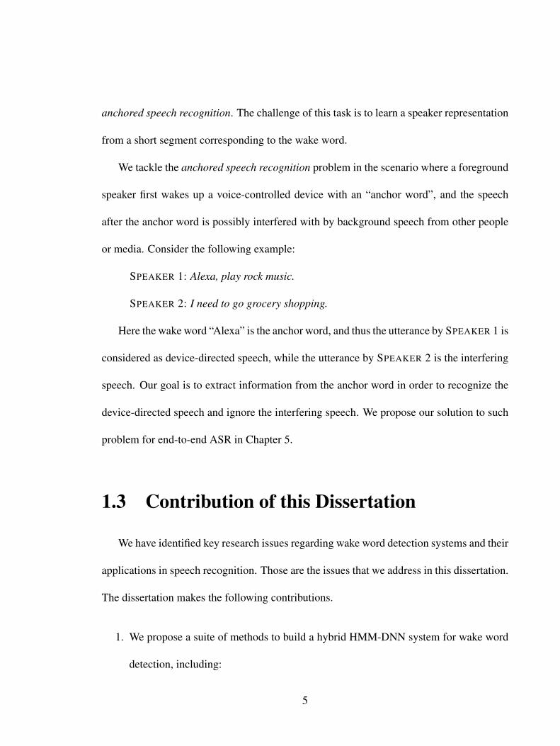
We tackle the anchored speech recognition problem in the scenario where a foreground
speaker first wakes up a voice-controlled device with an “anchor word”, and the speech
after the anchor word is possibly interfered with by background speech from other people
or media. Consider the following example:
SPEAKER 1: Alexa, play rock music.
SPEAKER 2: I need to go grocery shopping.
Here the wake word “Alexa” is the anchor word, and thus the utterance by SPEAKER 1 is
considered as device-directed speech, while the utterance by SPEAKER 2 is the interfering
speech. Our goal is to extract information from the anchor word in order to recognize the
device-directed speech and ignore the interfering speech. We propose our solution to such
problem for end-to-end ASR in Chapter 5.
1.3 Contribution of this Dissertation
We have identified key research issues regarding wake word detection systems and their
applications in speech recognition. Those are the issues that we address in this dissertation.
The dissertation makes the following contributions.
1. We propose a suite of methods to build a hybrid HMM-DNN system for wake word
detection, including:
5
(a) Sequence-discriminative training based on alignment-free LF-MMI loss, re-
moving the need for knowing the location of the wake word in each training
example.
(b) Whole-word HMMs for the wake word and filler speech, removing the need for
transcripts of the training speech or pronunciation lexicons.
(c) An online decoder tailored to the low latency constraints of the wake word
detection task.
The first two features significantly reduce model size and greatly simplify the train-
ing process, while the last one is suitable for a fast online detection. We evaluate
our methods on two publicly available real data sets, showing 50%–90% reduction
in false rejection rates at prespecified false alarm rates over the best previously pub-
lished figures, and re-validate them on a third (large) data set from an industry col-
laborator.
2. We explore the performance of several variants of chunk-wise streaming Transform-
ers tailored for wake word detection in the above LF-MMI system, including looking-
ahead to the next chunk, gradient stopping, different positional embedding methods
and adding same-layer dependency between chunks. We demonstrate that the pro-
posed Transformer model outperforms the baseline convolutional network by 25%
on average in false rejection rate at the same false alarm rate as a baseline model
6

with a comparable size, while still maintaining linear complexity w.r.t. the sequence
length.
3. We develop a fully parallelized PyTorch implementation of alignment-free LF-MMI
training for the streaming Transformer models, supporting GPU training on both
numerator and denominator graphs. It can be used for both wake word detection and
ASR, contributing to the broader speech research community.
4. We propose two encoder-decoder-with-attention (or named “attention-based
encoder-decoder”) models to tackle the anchored speech recognition problem using
information extracted from the anchored segment. The anchored segment refers
to the wake word part of an audio stream, which contains the speaker information
needed to suppress interfering speech and background noise.
(a) The first method is called Multi-source Attention where the attention mecha-
nism takes both the speaker information and decoder state into consideration.
(b) The second method directly learns a frame-level mask on top of the encoder
output.
(c) We also explore a multi-task learning setup where we use the ground truth of
the mask to guide the learner.
The proposed methods show up to 15% relative reduction in WER for Amazon Alexa
live data with interfering background speech without significantly degrading on clean
speech.
7

This dissertation is organized as follows. We firstly introduce necessary background
in Chapter 2, which includes traditional HMM-based and more recent neural end-to-end
speech recognition approaches, trained with either frame-level or sequence-level loss, dif-
ferent challenges that wake word detection has from speech recognition and how existing
wake word detection systems are therefore designed. In Chapter 3 we will detail our pro-
posed HMM-based wake word detection system, providing thorough experimental results
and analyses. Chapter 4 proposes a streaming version of Transformer neural networks and
demonstrate its effectiveness in acoustic modeling for wake word detection. Chapter 5
presents approaches for anchored speech recognition with the detected wake word segment
as an anchor. We finally make conclusions in Chapter 6.
8
Chapter 2
Background
2.1 Speech Recognition
Speech has been one of the most important ways for human to communicate with each
other and convey information and knowledge, since long before writing systems were in-
vented. Historically speech from people in important occasions or events were transcribed
into books manually. In our age, thanks to the development of information technologies,
computers can now do such a job quite well automatically. The task of speech transcription,
also known as automatic speech recognition (ASR) [146], refers to a computer program that
transcribes human speech from audio into text. Note that the ASR task does not involve the
process of “understanding” the content of speech. So a successful ASR system itself does
not necessarily imply that computers can, for example, take instructions from human, un-
9

derstand the intention, or respond appropriately. These problems are subjects of extensive
study in the current human language technology literature (e.g. [93], [142]).
Almost all successful ASR systems today tackle the problem from a probabilistic per-
spective. Mathematically, if we denote the observed audio as O (either the raw waveform
or a suitable predefined acoustic representation called “features”, e.g., spectrogram [33],
filter bank outputs [99], mel-frequency cepstral coefficients [78] (MFCCs), or perceptual
linear predictive [43] (PLP)) and its word transcription as𝑊 , the goal of ASR is to find the
most probable word sequence given O:
W∗ = arg maxW
𝑃(W|O) (2.1)
The process of finding the best sequence hypothesis as shown in Eq. (2.1) is called
“decoding” in ASR.
The ASR problem fits in the supervised learning paradigm, where given the input fea-
tures (here it is O), the machine learning model is trained to predict the label/class (here
it is W). There are generally two types of probabilistic models for supervised learning:
generative models and discriminative models, each of which represents one mainstream of
approaches to tackle the ASR problem today. In the next section we will introduce the
HMM based approaches as generative models. Our work on the wake word detection also
falls in this category. Then we will introduce the so-called “end-to-end” approaches most
10
of which are basically discriminative ones and have recently gain much popularity. Our
work on wake-word assisted ASR belongs to this category.
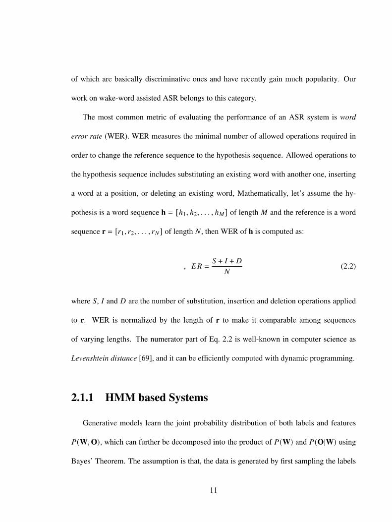
The most common metric of evaluating the performance of an ASR system is word
error rate (WER). WER measures the minimal number of allowed operations required in
order to change the reference sequence to the hypothesis sequence. Allowed operations to
the hypothesis sequence includes substituting an existing word with another one, inserting
a word at a position, or deleting an existing word, Mathematically, let’s assume the hy-
pothesis is a word sequence h = [ℎ1, ℎ2, . . . , ℎ𝑀] of length 𝑀 and the reference is a word
sequence r = [𝑟1, 𝑟2, . . . , 𝑟𝑁 ] of length 𝑁 , then WER of h is computed as:
𝑊𝐸𝑅 =𝑆 + 𝐼 + 𝐷
𝑁(2.2)
where 𝑆, 𝐼 and 𝐷 are the number of substitution, insertion and deletion operations applied
to r. WER is normalized by the length of r to make it comparable among sequences
of varying lengths. The numerator part of Eq. 2.2 is well-known in computer science as
Levenshtein distance [69], and it can be efficiently computed with dynamic programming.
2.1.1 HMM based Systems
Generative models learn the joint probability distribution of both labels and features
𝑃(W,O), which can further be decomposed into the product of 𝑃(W) and 𝑃(O|W) using
Bayes’ Theorem. The assumption is that, the data is generated by first sampling the labels
11

W from a prior probability distribution, and then generating the features O from a condi-
tional distribution given the labels. The parameters of 𝑃(W), 𝑃(O|W) are estimated from
training data. For prediction, by applying Bayes Rule, Eq. (2.1) can be rewritten as:
W∗ = arg maxW
𝑃(W|O) (2.3)
= arg maxW
𝑃(O|W)𝑃(W)𝑃(O)
= arg maxW
𝑃(O|W)𝑃(W)
In ASR, 𝑃(O|W) and 𝑃(W) are obtained from an acoustic model and a language model
respectively. Before decoding, a decoding graph, usually represented with a Weighted
Finite State Transducer (WFST, explained in the next section), is constructed to constrain
the search space with the language model [141]. During decoding, the score from the
language model will be combined with the score from the acoustic model to find the path
through the WFST with the best combined score among all permissible paths in the search
space. That best path corresponds to recognized word sequence.
The most widely used generative model for 𝑃(O|W) in ASR is the hidden Markov
model (HMM) [144], where the temporal dynamics of linguistic units are modeled via
transition probabilities under the Markov assumption, and acoustic features given linguistic
units are modeled via emission probabilities. Note that here we use the term “linguistic
units” rather than “words”, as practically, we do not directly use words as modeling units
in acoustic modeling due to data scarcity issue for very large vocabulary; instead finer-
12

granularity ones like phonetic [50] or graphemic [65] units L are used with a lexicon as:
𝑃(O|W) =∑
L∈L(W)𝑃(O|L)𝑃(L|W) (2.4)
where L(W) is the set of all possible phonetic/graphemic sequences corresponding to the
word sequence W. 𝑃(L|W) is static and is usually given by a lexicon, while 𝑃(O|L) can
be considered as the probability of the frame sequence under a long HMM concatenated
from several small HMMs each of which corresponds to a subword unit (e.g., phoneme or
grapheme, etc) in L:
𝑃(O|L) =∑
S∈A(L)𝑃(O, S|L) =
∑S∈A(L)
𝑇∏𝑡=1
𝑃(𝑜𝑡 |𝑠𝑡)𝑃(𝑠𝑡 |𝑠𝑡−1) (2.5)
where A(L) is the set of all possible HMM state sequence of length 𝑇 subject to 𝐿,
𝑃(𝑜𝑡 |𝑠𝑡) is the emission probability of 𝑜𝑡 given the state 𝑠𝑡 , and 𝑃(𝑠𝑡 |𝑠𝑡−1) is the transition
probability from 𝑠𝑡−1 to 𝑠𝑡 in HMMs. Note that the states as random variables are unob-
served (hidden), so the summation over these random variables in Eq. (2.5) is needed to
marginalize all possible values.
2.1.1.1 Weighted Finite-state Transducers
First we introduce finite-state automaton (FSA) [34]. An FSA defines a directed graph
which accepts a set of strings. The nodes in the graph represent states and the arcs be-
13

tween nodes represent transitions between these states. Formally, an FSA is a 5-tuple
(𝑄,Σ, 𝐼, 𝐹, 𝛿) such that:
• 𝑄 is a finite set of states;
• Σ is a finite set of input alphabet;
• 𝐼 is a subset of 𝑄 representing initial states;
• 𝐹 is a subset of 𝑄 representing final states;
• 𝛿 ⊆ 𝑄 × (Σ⋃𝜖) ×𝑄 is the set of transitions, where 𝜖 is the empty string meaning
“no symbol”.
A weighted finite-state automaton (WFSA) is an extension of FSA where a weight is
associated with each transition and optionally with initial and final states, so that each ac-
cepted string has an associated weight which is the “multiplication” of all weights along the
path corresponding to that string. Note that “multiplication”, along with another operation
“addition”, is defined in an algebraic structure named “semiring” [82].
A finite-state transducer (FST) [52] is a generalization of an FSA, where it defines
relations of two sets of strings. In addition to a set of input strings that an FSA accepts,
an FST defined another set of output strings that input strings map to. An FSA can be
seen as a special case of an FST when the input and output set of strings are identical and
the mapping is the identity function. Similarly, FST can also been extended to Weighted
Finite-state Transducer (WFST). Therefore, a WFST can be defined on top of a WFSA as
14

an 8-tuple (𝑄,Σ, Γ, 𝐼, 𝐹, 𝛿, _, 𝜌) with 𝑊 being the set of weights, where 𝑄,Σ, 𝐼, 𝐹 are the
same as the definitions above, and:
• Γ is a finite set of output alphabet;
• 𝛿 ⊆ 𝑄 × (Σ⋃𝜖) × (Γ⋃𝜖) ×𝑄 ×𝑊 is the set of transitions, where 𝜖 is the empty
string meaning “no symbol”;
• _ : 𝐼 → 𝑊 is the mapping from initial states to weights;
• 𝜌 : 𝐹 → 𝑊 is the mapping from final states to weights.
composition is an operation defined on two FSTs1. If FST 𝐴 transduces string 𝑥 to
𝑦 and FST 𝐵 transduces string 𝑦 to 𝑧, then the composition 𝐴 𝐵 transduces string 𝑥 to
𝑧. Composition is important in speech recognition because it is able to combine different
granularity levels of symbols together. For example, as mentioned in Section 2.1.1, the
decoding graph is represented as an FST, which is a composition of 4 FSTs: 𝐻 𝐶 𝐿 𝐺.
𝐻 is an HMM (represented as an FST) that transduces phone states to context-dependent
phones (see Figure 2.1 for an example FST transducing all allowed phone state sequences
to one context-dependent phone). 𝐶 is an FST that transduces context-dependent phones
to context-independent (mono-) phones. 𝐿 is a lexicon transducing mono-phones to words.
𝐺 is a language model, which is usually an FSA specifying the probability of an accepted
word sequence. Therefore, composition allows the decoding graph to directly transduce a
phone state sequence to a word sequence with an associated weight as a “score” measuring1The remaining of this dissertation will use the terminology “FST” and “WFST” interchangeably to refer
to weighted finite-state transducer if not otherwise specified, following the convention in speech recognition.
15

how likely each word sequence would be. Interested readers may refer to [82] for more
details on how WFSTs are used in speech recognition.
0
0:0
11:1
0:0
22:0
0:0
33:0
0:0
44:0
Figure 2.1: An example FST transducing phone state sequences to a phone indexed with 1.Every arc represents a transition, and the pair of numbers associated with an arc are indexesof pdf-ids (used for emissions in HMMs) and a phone respectively (0 is the index of blankin the input and the index of 𝜖 in the output). So this FST defines a phone with 4 pdf-ids.
2.1.1.2 Deep Neural Networks for Acoustic Modeling
Traditionally Gaussian mixture models (GMM) [5] were used to estimate the emission
probabilities 𝑃(𝑜𝑡 |𝑠𝑡) in HMMs, in which case the whole model is called “HMM-GMM”.
With the recent success of deep learning and advances of graphics processing units (GPUs),
deep neural networks (DNN) have replaced GMMs [45] because of their stronger modeling
power. Such “HMM-DNN” models are referred to as “hybrid systems” in literature as they
are hybrid of two different types of probabilistic models: a Bayesian network [62] (i.e.
HMM) and a neural network.
The transition probabilities in HMM-DNN models are usually obtained from a prior
training stage (e.g. HMM-GMM training), and the neural network can be trained either
16

with a frame-level loss or a sequence-level loss. If trained with a frame-level loss (e.g.,
cross-entropy loss), the output of the neural network DNN can be roughly interpreted as
the conditional probability 𝑃(𝑠𝑡 |𝑂) for the frame at time step 𝑡2. However the frame-level
label 𝑠𝑡 are not directly available from the ASR training transcripts (i.e., word sequence).
On the other hand, research (e.g. [45]) has shown that HMM-GMM models could provide
reliable estimate of the HMM state occupancy for each frame. Therefore, 𝑠𝑡 is inferred from
a trained HMM-GMM model3 via a process called “forced alignment”, and is actually the
result of performing Viterbi decoding [125]. Note however that what we actually need in
Eq. 2.5 is 𝑃(𝑜𝑡 |𝑠𝑡), which can be obtained by resorting to Bayes Rule again:
𝑃(𝑜𝑡 |𝑠𝑡) ∝𝑃(𝑠𝑡 |𝑜𝑡)𝑃(𝑠𝑡)
(2.6)
where the state prior 𝑃(𝑠𝑡) is estimated from the forced alignment of the entire training
scripts produced by HMM-GMM models.
Neural networks used for acoustic modeling have also been evolved over the past years.
The name “DNN” initially refers to a type of neural networks with several feed-forward
layers [45], where each layer can be described as
y = 𝜎(Wx + b) (2.7)
2We use “roughly” to emphasize that the neural output cannot be interpreted exactly the same way as thecorresponding probability in GMM.
3The HMM-GMM model itself is trained with the Expectation-Maximization algorithm [5].
17

where x ∈ R𝑑𝑖𝑛 is the input to the layer, y ∈ R𝑑𝑜𝑢𝑡 is the output, W ∈ R𝑑𝑜𝑢𝑡×𝑑𝑖𝑛 , b ∈ R𝑑𝑜𝑢𝑡
are trainable parameters (or “weights”), and 𝜎(·) is an activation function which is usu-
ally implemented as an element-wise non-linearity function, e.g. Rectified Linear Unit
( 𝑓 (𝑥) = 𝑥 if 𝑥 ≥ 0 or 0 otherwise) or Sigmoid ( 𝑓 (𝑥) = 11+𝑒 (−𝑥) ). According to universal
approximation theorem [25], [47], a multilayer feed-forward neural network, with an arbi-
trary number of artificial neurons or layers, is a universal approximator of any continuous
function. This implies neural networks can represent various functions with appropriate
weights. However, this theorem does not give how to construct such networks given a
specific task, and people need to try different types of hand-crafted neural networks for
different tasks 4.
Inspired by the success of conventional networks in hand-written digit recognition [66]
and natural image recognition [40], researchers found convolutions can also better model
the speech data and perform better than feed-forward networks [1]. In convolutions, con-
volution kernels are defined to capture local patterns of speech features (e.g., spectrgram
or filterbanks). The kernel slides along time axis (1D convolutions) or additionally along
frequency axis (2D convolutions), outputting a large value if a local pattern matches that
kernel:
𝑔(𝑥, 𝑦) = W ∗ 𝑓 (𝑥, 𝑦) =𝑚∑
𝑑𝑥=−𝑚
𝑛∑𝑑𝑦=−𝑛
W(𝑑𝑥, 𝑑𝑦) 𝑓 (𝑥 + 𝑑𝑥, 𝑦 + 𝑑𝑦) (2.8)
where ∗ is the convolution operator, W is the kernel of size (2𝑚 + 1) × (2𝑛 + 1), 𝑓 (𝑥 − 𝑑𝑥 :
𝑥 + 𝑑𝑥, 𝑦 − 𝑑𝑦 : 𝑦 + 𝑑𝑦) is a patch centered at (𝑥, 𝑦), and 𝑔(𝑥, 𝑦) is the output value at (𝑥, 𝑦).4Recently there is some work on neural archtecture search [31] to automate this process.
18

Note that the definition of convolution in machine learning applications (e.g. computer
vision and speech recognition) is actually a “flipped” version of that in signal processing:
in signal processing convolution is defined as:
𝑔′(𝑥, 𝑦) = W ∗ 𝑓 (𝑥, 𝑦) =𝑚∑
𝑑𝑥=−𝑚
𝑛∑𝑑𝑦=−𝑛
W(𝑑𝑥, 𝑑𝑦) 𝑓 (𝑥 − 𝑑𝑥, 𝑦 − 𝑑𝑦) (2.9)
where the signs before 𝑑𝑥 and 𝑑𝑦 in 𝑓 (·, ·) are negative. The procedure of repeatly applying
the kernel at different location of the input is designed to be able to extract shift-invariance
features from the input, as local patterns at different location lead to the same output value.
More global patterns (or long-range dependency in sequence data like speech) will be cap-
tured by stacking multiple convolution layers together. The more the layers, the more input
the output can “see”. Here we introduce the concept of receptive field, which will also be
used in later chapters. Receptive field is defined as the size of the region in the input that
produces an output. It measures the association of an output of a neural network to the input
region, and a larger number means the output needs to rely more input frames to compute a
value. For example, a single convolution layer with a kernel size 3 has the receptive field of
size 3 × 3, and a network consisting of two such convolution layers has the receptive field
of size 5 × 5.
The time delay neural network (TDNN) was first introduced for phoneme classification
[126] using features representing a pattern of unit output and its context from the previous
layer. It is equivalent to convolution with “dilated” convolution kernels. “Dilated” means,
19

instead of applying the kernel on a contiguous input region, the kernel is applied to a dilated
region where every 𝑘-th input in a patch is involved in the computation:
𝑔(𝑥, 𝑦) = W ∗ 𝑓 (𝑥, 𝑦) =𝑚∑
𝑑𝑥=−𝑚
𝑛∑𝑑𝑦=−𝑛
W(𝑑𝑥, 𝑑𝑦) 𝑓 (𝑥 + 𝑘 · 𝑑𝑥, 𝑦 + 𝑘 · 𝑑𝑦) (2.10)
TDNN was later applied to acoustic modeling for ASR [39], [91], [92] and speaker recog-
nition [114], and was demonstrated to be robust to speech recognition with different rever-
beration levels. The “dilation” also provides a way of enlarging the receptive field without
increasing the number of parameters.
Although convolutional networks have the capacity of modeling long-range depen-
dency for sequence data, it is later found to be less effective than another type of neural
networks named recurrent neural networks (RNN) with its more sophisticated variants
such as Long-short Term Memory (LSTM) [46] and Gated Recurrent Units (GRU) [19]
networks. Mathematically, an RNN defines a recursive computation along the time axis:
𝑠𝑡 = 𝑓 (𝑠𝑡−1, 𝑥𝑡) (2.11)
where 𝑠𝑡 is the hidden state at 𝑡 and 𝑥𝑡 is the input at 𝑡. At any time 𝑡, the network compute
the new state at 𝑡 based on the old state 𝑠𝑡−1 and the new input 𝑥𝑡 . Hence an RNN can the-
oretically encode arbitrary long history of information into a fixed-length vector. However
in practice, a carefully designed network architecture (e.g. LSTM or GRU) and training
20

strategy (e.g. gradient clipping) are needed to avoid the gradient explosion/vanish problem
[46] when the sequence length is long.
Recently self-attention [123] has shown its superior performance in both NLP and
speech communities for its capability of modeling long-range dependency for sequence
data without recurrent connections. In self-attention each frame directly interacts with
other frames within the same layer, making each frame aware of its contexts, i.e. for a
given frame 𝑖, its output 𝑦𝑖 is the weighted sum of all the hidden state ℎ 𝑗 in the same layer:
𝑦𝑖 =∑𝑗
𝑤𝑖, 𝑗ℎ 𝑗 (2.12)
where the weight 𝑤𝑖, 𝑗 is determined by the similarity between frame 𝑖 and frame 𝑗 . Owing
to the direct connections between frames, the gradient paths are much shorter while back-
propagating, alleviating gradient explosion/vanishing problems commonly seen in recur-
rent networks.
2.1.1.3 Training with HMMs
The HMM is a generative model, in the sense that the there exists a generative process
specified by the model for describing the observation O. The training method aims to
21

maximize the observation’s likelihood given the HMM. If we ignore the the intermediate
linguistic units, the training can be expressed as:
max\
∑𝑢
log 𝑃(O𝑢 |W𝑢; \) (2.13)
where \ represents the model parameters, and 𝑢 indexes the training utterances. This way
of learning the model through Eq. (2.13) is called Maximum likelihood estimation (MLE).
Some generative models, like HMM, can also be trained discriminatively. For exam-
ple, in some discriminative training of the HMM, we are trying to maximize the posterior
probability of labels W𝑢:
max\
∑𝑢
log 𝑃(W𝑢 |O𝑢; \) = max\
∑𝑢
log𝑃(O𝑢 |W𝑢; \)𝑃(W𝑢)
𝑃(O) (2.14)
= max\
∑𝑢
log𝑃(O𝑢 |W𝑢; \)𝑃(W𝑢)∑W 𝑃(O𝑢 |W; \)𝑃(W)
where the numerator in Eq. 2.14 computes the probability assigned by the model to the
reference label W𝑢, while the denominator computes the probability over all possible label
sequences (called “competing hypotheses”). By comparing Eq. 2.14 with Eq. 2.13, we can
see that, rather than only making the “correct” sequence more likely, the discriminative
training also learns to make “incorrect” sequences less likely. In other words, the model
is trained to maximize the separation between the correct and incorrect answers. Note that
both the numerator and denominator involve the probability of label sequence 𝑃(W), which
22

means that the discriminative training also takes linguistic information into consideration.
That is why the discriminative training is typically seen to have better performance than
the MLE training, especially when the training data is relatively small.
There are several specific discriminative training criteria for ASR, including Maximum
Mutual Information (MMI) and Minimum Phone Error (MPE) [94]. They share similar
spirit, and the main difference lie in what quantity (e.g., mutual information or phone error)
is being used as criteria. We use MMI for the exposition above, as it is directly related to
the work in this dissertation.
In the straightforward implementation of MMI training, competing hypotheses being
used in the denominator are usually compactly represented as a word lattice. A lattice is
a directed acyclic graph representing a set of likely word sequences for an utterance, with
various information associated with the arcs and/or nodes (e.g., in Kaldi [96] a lattice is a
special WFST, where acoustic model score and language model score are separately stored
on arcs). A word lattice contains a set of finite number of word sequence hypotheses after
decoding with a decoding graph, so it is just an approximation of the whole hypothesis
space [14]. Also, it requires a pretrained model to be generated. One may also consider
using a word-based denominator graph in the denominator of Eq. (2.14). However, the
word vocabulary size is usually in the tens of thousands, making the forward probabilities
required by forward-backward algorithm unable to fit in GPU memory. To resolve this
issue, Lattice-free MMI [98] (LF-MMI) was proposed, where an “exact” phone-level lan-
guage model is used to construct the denominator graph. Because the phone inventory size
23

of a language is much smaller than the word vocabulary size (typically less than 100), the
computation of the denominator sum in Eq.( 2.14) can efficiently be carried out on GPUs.
2.1.2 Neural End-to-end Systems
The HMM-DNN hybrid systems introduced in the previous section have improved
WERs significantly over the last decade. Some ASR systems can even reach “human par-
ity” on some benchmarks [105], [139]. However, the hybrid systems involve independently
trained components, namely acoustic, language, and pronunciation/spelling models, lead-
ing to a complicated pipeline and possibly sub-optimal performance. Also, due to the large
size of the language model used to build the decoding graph, it is not easy to perform on-
device inference with limited memory. To address these problems, recent work in ASR
begun paying attention to so-called neural end-to-end systems [7], [21], [37], which are
characterized by generally smaller code size, and greater portability and maintainability
across hardware platforms and software environments.This shift is analogous to the one in
the machine translation (MT) community: from feature- and syntax-based statistical ma-
chine translation (SMT) systems (e.g. Moses [61], Joshua [71]) to end-to-end neural ma-
chine translation (NMT) systems (e.g. OPENNMT [58], OPENSEQ2SEQ [63], FAIRSEQ
[86]).
All such neural end-to-end systems are trying to learn a sequence-to-sequence model.
Let’s denote the input sequence as 𝑋 = 𝑥1, 𝑥2, . . . , 𝑥𝑇 , and output sequence as 𝑌 =
𝑦1, 𝑦2, . . . , 𝑦𝑈 , where 𝑈 is not necessarily equal to 𝑇 . What these models do is to learn
24

a mapping function 𝑓 : 𝑋 → 𝑌 using a properly designed neural network. One major
difficulty in finding such a mapping function is how to learn the alignment between the
input frames and output labels. Most HMM-DNN based systems tackle this problem by
the forced alignment (see Sec. 2.1.1.2). For neural end-to-end systems, since there are
no existing models which can be used to generate such alignment, the model itself has to
simultaneously infer the alignment and the mapping function with the alignment. Differ-
ent from the HMM based models, most of the neural end-to-end models are discriminative
models, as they learn the conditional probability 𝑃(𝑌 |𝑋) as opposed to the joint probability
𝑃(𝑋,𝑌 ).
The earliest neural end-to-end ASR systems were trained with the so-called connec-
tionist temporal classification (CTC) loss [36], [37]. There is a single network in such
systems that encodes the input feature frames 𝑋 into an intermediate representation, and
all possible alignments 𝐴 corresponding to the reference transcript are marginalized to give
the conditional probability:
𝑃(𝑌 |𝑋; \) =∑
𝐴∈B−1 (𝑌 )𝑃(𝐴|𝑋; \) (2.15)
where B(·) is the many-to-one function that maps an alignment to its corresponding tran-
script. B−1(𝑌 ) thus specifies all possible alignments for a reference𝑌 . It assumes the output
length 𝑈 is not longer than the input length 𝑇 5, and a special blank symbol is introduced
to output transcriptions of shorter lengths (𝑈 < 𝑇). B(·) is simply achieved by collapsing
5There are other assumptions, like monotonic alignments which is satisfied in ASR.
25

repeats and then removing all the appearances of the blank symbol from 𝐴. The sum in
Eq. 2.15 is efficiently computed using the forward-backward algorithm, similar to the one
used in HMMs.
One disadvantage that CTC has is given the input 𝑋 , that the output symbols at each
time step are conditionally independent of each other, i.e., the prediction at time 𝑡 will not
be affected by predictions from any other time steps. Such a assumption does not hold
in ASR. Therefore, a separate language model, adding back the statistical dependence, is
needed to improve the decoding results.
Some work argue that the property of conditional independence in CTC is beneficial
while adapting to a new language domain [79], [80]. However, there is still the belief
that a jointly trained model with both acoustic and language components is preferable in
terms of ASR performance. To overcome the conditional independence assumption of
the CTC model, two novel models have been proposed. The first one is called “RNN
Transducer” (RNN-T) 6 [35]. Compared with CTC, besides the encoder network 𝑓enc,
RNN-T has an additional so-called prediction network 𝑓pred, which is analogous to auto-
regressive RNNLMs [81], to model the conditional dependency among predicted symbols.
6The name is a bit confusing. There is no limitation to the type of the neural network being used. ActuallyTransformers have been recently adopted as its encoder in lieu of a recurrent neural network (RNN) to obtainbetter results [10], [143], [148].
26

In addition, a joint network combines the the output from the encoder and the prediction
network to compute the alignment scores:
y𝑢,𝑡 = 𝑓joint(q𝑢, s𝑡) (2.16)
where q𝑢 is the hidden state of the 𝑢-th step of the predictor network 𝑓pred, and s𝑡 is
the 𝑡-th frame of the output of encoder network 𝑓enc. Different from those in CTC, RNN-
T allows emissions of multiple symbols for each input frame. The loss is computed by
forward-backward algorithm as well, taking both the acoustic and language information
into account.
Both CTC and RNN-T work in a frame-synchronized way, meaning that predictions
are made on every frame. On the contrary, the second type of model overcoming the con-
ditional independence is the encoder-decoder with attention model. It works in a label-
synchronized manner, i.e, symbols are not emitted on each frame, and there should be a
special end-of-sentence symbol indicating the termination of the prediction during decod-
ing. This type of model was originally proposed for Neural Machine Translation (NMT)
[3], [74], and was then successfully pioneered by [21] in the speech community. It consists
of three modules: an encoder network 𝑓enc, a decoder network 𝑓dec, and an attention net-
work 𝑓att. What distinguishes itself most from CTC or RNN-T is that the model introduces
an attention mechanism to guide the decoder network 𝑓dec to pay attention to a specific part
27

of the output of the encoder network 𝑓enc while making a prediction:
𝛼𝑢,𝑡 = Attention(q𝑢, s𝑡) (2.17)
c𝑢 =∑𝑡
𝛼𝑢,𝑡s𝑡 (2.18)
where 𝛼𝑢,𝑡 indicates how much attention q𝑢 in the decoder should pay to s𝑡 in the encoder.
Attention(·) represents the attention module, which can be implemented as Bahdanau At-
tention [2] or Luong Attention [74]. Both of them are to compute some kind of affinity
score between q𝑢 and s𝑡 . The difference is that former one adds the transformed q𝑢 and s𝑡
vector together:
𝜔𝑢,𝑡 = v⊤ tanh(W𝑞q𝑢 +W𝑠s𝑡 + b) (2.19)
while the latter one use the dot-product of the two vectors:
𝜔𝑢,𝑡 = q⊤𝑢 W𝑞⊤W𝑠s𝑡 (2.20)
The similarity scores are then normalized by softmax function to obtain the valid proba-
bility 𝛼𝑢,𝑡 :
𝛼𝑢,𝑡 = softmax(𝜔𝑢,𝑡) (2.21)
At every decoder time step, it not only relies on the previously predicted symbol (sim-
ilar to the prediction network in RNN-T), but also on the information provided by the
encoder and the attention module. The attention module tells the decoder, given the current
28

decoding state, what portion of the input feature is most useful, by making a summary of
the useful portion:
q𝑢 = 𝑓dec(q𝑢−1, [𝑦𝑢−1; c𝑢−1]) (2.22)
where q𝑢 is the decoder state at the 𝑢-th step, 𝑦𝑢−1 is the output from the the 𝑢 − 1-th step,
and c𝑢−1 is the summary vector computed from the attention and encoder for the this step.
This attention mechanism is key to the anchored speech recognition task, as will be detailed
in Chapter 5.
2.2 Wake Word Detection
Similar to ASR, approaches to wake word detection can also be categorized into two:
1) HMM-based keyword-filler models; and 2) pure neural models. However, due to the
much more restricted computational resources and the low latency requirement discussed
in Chapter 1, existing methods from large-vocabulary ASR cannot be directly applied to
wake word detection. Specifically:
• In ASR, the modeling units are usually tri-phones/bi-phones in HMM-based systems,
or wordpieces/words in neural end-to-end systems. So the vocabulary size is at least
several thousands, making the model size and computation cost prohibitive for wake
word detection.
29
• Datasets for wake word detection are usually collected and prepared in a way that
rich transcripts are unavailable, both because of the difficulty of the transcription
given the poor quality of recordings collected from challenging environments, and
lack of necessity of doing so as the task is not to recognize all the words, but just
assert the presence of the wake word. This affects the design of models.
• For HMM-based ASR, a word lattice is generated by expanding the decoding graph
based on the acoustic score of each frame. The lattice is needed so that it can be
rescored with a stronger word language model to obtain better results [140]. For
wake word detection, because of its very limited word vocabulary, the word language
model is extremely simple and a lattice is not needed for rescoring with a word
language model.
• While offline decoding is admissible in some ASR applications, for wake word de-
tection, we do not want to wait until the current recording has finished for decoding.
Instead we want to start decoding as soon as the audio stream is available, and report
the positive trigger immediately once the wake word is spotted. This will affect both
the model design and the decoding strategy.
There is no definitive conclusion about whether the pure neural systems are better than
HMM-based ones. Note that for ASR, HMM-based systems have the disadvantage that the
decoding graph could take up large space in memory usage. However, this is not a problem
for wake word detection, as the decoding graph is orders of magnitude smaller.
30

2.2.1 HMM-based Wake Word Detection Systems
The existing way of decoding HMM-based wake word systems is basically similar
to that for ASR: usually conducted through Viterbi search where multiple high scoring
partial paths are maintained at each frame, and extended synchronously using dynamical
programming. To speedup the decoding process and reduce the computation cost, beam
search is commonly adopted: only partial paths with their scores within a predefined beam
width of the best one are considered for extension, and their scores are incremented with
both the frame-wise acoustic score and the “language model” score on the arc it chooses
to extend with from the graph. Once all frames are consumed, the best path on the graph
is traced back to determine the presence of the wake word. In [138] two decoding graphs
are constructed: the foreground graph for the wake word, and the background graph for
non-wake-word. The difference of the scores obtained with the two graph is used for the
decision. We will introduce a different strategy in Chapter 3, considering all the partial
hypotheses in the beam for making the detection decision.
The classical HMM-based keyword-filler models, representing both the keyword and
filler (background) models, for KWS are discussed in [102], [103], [118]. The keyword
model consists of all valid phone sequences from the keyword, and the filler model includes
all other speech and non-speech. During the decoding phase, usually the ratio of the scores
with keyword graph and with the filler graph is computed for determining the presence of
the wake word. With recent advances in deep learning, HMM-DNN hybrid wake word
systems replace GMM-based acoustic models with a neural network to classify individual
31

frames [87], [117], [138]. While the filler model for background speech is specified as
having an ergodic topology between speech and non-speech in [87], [117], it is represented
as an all-phones loop in [138], increasing both the neural network model size and decoding
graph size due to the increased number of modeling units. Finally, some methods add
automatic speech recognition (ASR) as an auxiliary task during training [117]. In Chapter
3 we will show that it suffices to use a much smaller number of output units than the number
of all phones’ states, with which we can remove the need to specify a pronunciation lexicon.
2.2.2 Pure Neural Wake Word Detection Systems
Pure neural models abandon HMMs and completely rely on neural networks for acous-
tic modeling, where the subwords or even whole words of the wake word phrase (wake
phrase, for short) are directly used as modeling units. The first successful wake word de-
tection systems of this type were proposed in [8], [104]. They use individual words in the
wake phrase as the modeling units to reduce the network size. However, they still need a
forced alignment of the training audio with its transcripts, obtained from an existing HMM-
based ASR system, to form training examples for the wake word system, which limits the
applicability of their methods if an ASR system is unavailable. For decoding, they adopt
a fast posterior handling approach where the posterior probability of words is smoothed
within a sliding window over the audio frames. [24], [83] use the whole wake phrase as
the training target, but they still need phone-level alignments to pretrain a small network
before being fine-tuned with word targets. There are also several proposals that do not re-
32

quire frame-level alignment for training, including max-pooling [49], [116], the attention
mechanism [108], [129], and global mean-pooling [4]. More recently, RNN-transducer
and attention based models have been investigated for KWS/wake word detection [4], [41],
[108].
It has been shown that some sequence-level training criteria perform better than some
frame-level criteria for ASR. The output in a wake word detection task, by contrast,
is relatively simple. However, if the modeling units are subwords (e.g., phonemes or
HMM states), wake word detection may still be considered as a sequence prediction task.
Sequence-level discriminative training such as CTC loss [36] has been explored for the
wake word detection task with graphemes or phonemes as subword units [32], [68], [136],
[151]. Lattice-free maximum mutual information (LF-MMI) is an HMM-based sequence-
level loss first proposed in [98] for ASR. In the context of wake word detection, it is re-
cently investigated in [15], where it still requires alignments from a prior model like an
HMM-GMM system to generate numerator graphs.
2.2.3 Neural Networks
Recurrent neural networks, such as LSTMs, GRUs and their variants may not be the
best choice for wake word detection due to latency considerations. Also for wake word
detection, the importance of long range temporal dependency may not be as large as in
ASR. Therefore, convolution-like or time-constrained self-attention are preferable as both
of them are highly parallelizable. Convolutional networks increase their receptive field by
33
stacking multiple layers together, with higher layers “seeing” more input frames, and self-
attention directly computes the relationship of the neighboring frames at the same layer
without the traditional recurrent connections. The number of future input frames that a
model depends on, i.e. look-ahead, should also be controlled for latency purposes.
Recently self-attention [123] has received popularity in both NLP and speech commu-
nities for its capability of modeling context dependency for sequence data without recurrent
connections. Self-attention replaces recurrent connections with direct interactions across
time within the same layer, making each frame aware of its context. Also, the gradient
paths are much shorter while back-propagating, alleviating gradient explosion/vanishing
problems commonly seen in recurrent networks. The computations are more easily par-
allelizable, in the sense that the computations of later frames do not depend on those of
previous frames in time. However, the original self-attention require the entire input se-
quence to be available before the global attention can be executed. Moreover, the vanilla
self-attention does not have a mechanism for saving the current computed states for future
reuse, and thus does not support the scenario of streaming inference for wake word detec-
tion. Time-restricted self attention [97] allows the self-attention to be restricted within a
small context window around each frame, which is preferable in our task as it can restrict
the attention to be only focused within limited contexts to achieve low latency. But it is
not a streaming model without the ability of caching history states. Transformer-XL [26]
consumes the input sequence in a chunk-wise fashion: the state from the previous chunk is
cached for the next chunk to attend to, which is suitable for streaming inference. It is not
34

clear, however, whether this advantage still holds for short-range temporal modeling like
wake word detection. So we will explore and discuss this aspect in Chapter 4.
2.2.4 Metrics
There are two major metrics for the evaluation of the wake worc detection performance:
equal error rate (EER) and false rejection rate (FRR) at a pre-specified false alarms per
hour (FAH). EER is obtained at an operating point on the Receiver Operating Character-
istic (ROC) curves as a scalar value at which the false rejection rate and the false alarm
rate are equal. This metric has been widely adopted in many other fields including biol-
ogy, medicine, statistics, etc., where binary classification is performed. In the wake word
detection scenario, people care more about, “the proportion of falsely rejected actual wake
word occurrences, while false alarms should only take place less than a specific number of
times per hour of negative data”. Therefore, the value of FRR at some pre-specified value
of FAH is usually reported for evaluation. A typical specification is between 0.1 and 1.0
for FAH.
2.3 Target Speaker ASR
In many real world scenarios, recordings obtained for ASR are not clean. Besides envi-
ronmental noise and reverberation caused by the imperfect recording devices and room
acoustics, there may also exist interfering speech from other speakers and background
35

noise. One example is in a multi-party meeting, where multiple talkers speak alternately,
and sometimes simultaneously. Another example is when a person is speaking to a voice-
controlled device, other people or devices like television in the background may also make
speech-like sounds, and such noise is undesirable to the voice-controlled device. Hence
there is a practical demand to perform ASR only for desired speaker from a recording con-
taining speech of multiple speakers, or mixture of speech and non-speech, while ignoring
other interfering speech or noise. We call this task “target-speaker ASR”.
One related task is speech separation 7, where each source of speech is to be isolated
from the mixture of speech before doing ASR. The common approach is to estimate a time-
frequency mask for each source in the mixture. This includes those directly estimating the
speaker-dependent mask with a deep neural network [127], [128], and those clustering the
embeddings of time-frequency bins for different speakers [16], [44]. The former ones re-
quire the neural network to have a fixed number of outputs and suffer from the permutation
problem [44], while the later ones do not suffer from those problems and postpone the time
of specifying the number of sources to the clustering stage. Another approach is using
“permutation invariant training” (PIT) [145], [147], which resolves the permutation prob-
lem within utterances but not across utterances. However, it still requires a predefined and
fixed number of the network’s outputs.
To perform target-speaker ASR, i.e., only recognizing the desired speaker’s speech
given some additional information about the speaker, the challenges are two-fold. One
7The problem is also famously referred to as “cock-tail party problem” [17].
36

is how to provide a good speaker representation (speaker identity or speaker characteris-
tics) that is distinctive and representative among other speakers. And the other is how to use
that speaker representation to extract and recognize the target speaker’s speech. A couple
of techniques have been proposed for learning speaker representations, e.g., ivector [27],
[106], mean-variance normalization [72], maximum likelihood linear regression (MLLR)
[67]. With the recent progress in deep learning, neural networks are used to learn speaker
embeddings. for speaker verification/recognition [42], [77], [115], [122]. There are several
methods for adapting the acoustic models with such speaker embedding vectors, and some
of them simply concatenate these vectors with the input features or intermediate neural
network outputs [55], [106], [107], [124], or adapt network parameters to speakers [84].
However, concatenation or biasing parameters does not provide a direct mechanism to only
focus on the target speaker and suppress other interfering/background speech. In addition,
off-the-shelf speaker embeddings learned separately may not be optimal for a downstream
task like target-speaker ASR.
Work that jointly trains the speaker embedding and the acoustic model for target speak-
ers can be found in [28], [53], [152]. In [152], all sub-layers of the speaker adaptive layer
are summed with learned weights to extract speech from the target speaker, where the
weights are determined from the speaker embedding learned from an adaptation utterance,
a short sample of speech from the target speaker. Then [28] extends that idea for target-
speaker ASR in hybrid systems, and it also demonstrates that joint training of the speaker
embedding and the acoustic model is more beneficial compared with separate training. [53]
37

adds an auxiliary loss for interference speakers to further improve the ASR performance.
In their experiments, however, target utterances are contiguous in the mixture of speech,
i.e., no interruptions by the background speech/noises. Specifically, if an utterance contains
segments without speech from the target speaker at all, and these segments are interleaved
with the segments containing only the target speaker, then there is no explicit mechanism
to skip those segments during decoding, as the output of all the frames will be used for
decoding.
Wake word segments have also been used to extract the speaker embeddings [55],
[75]. Two methods—anchor mean subtraction (AMS) and an encoder-decoder network—
are proposed to detect desired speech by extracting speaker characteristics from the wake
word [75]. This work is further extended for acoustic modeling in hybrid ASR systems
[55]. However, as mention above, its concatenation of the embedding to the input does not
empower the model with enough capacity.
In Chapter 5, we propose a unified architecture based on attention-based encoder-
decoder ASR model that uses wake word segments as an additional input for target-speaker
ASR. It relies on the attention mechanism over the encoder output, to explicitly select
frames belonging to the desired speaker. As a result, only the speech from the person who
speaks the wake word is recognized, and other speech and noise are ignored.
38
Chapter 3
Wake Word Detection with
Alignment-Free Lattice-Free MMI
This chapter first briefly introduces how Lattice-Free maximum mutual information
(LF-MMI) training works, and explains why it needs alignments for training, and then
presents our proposed wake word detection system, including the HMM topology, training
criterion, acoustic modeling, data preprocessing and augmentation, and online decoding.
The contributions of this work are: (i) we remove the prerequisite of frame-level alignments
in the LF-MMI training algorithm, permitting the use of un-transcribed training examples
that are annotated only for the presence/absence of the wake word; (ii) we show that the
classical keyword/filler model must be supplemented with an explicit non-speech (silence)
model for good performance; (iii) we present an FST-based decoder to perform online
detection. We evaluate our methods on two real data sets, showing 50%–90% reduction
39

in false rejection rates at prespecified false alarm rates over the best previously published
figures, and re-validate them on a third (large) data set. We also provide detailed analyses
of our proposed system, including how different model and receptive field sizes affect the
performance, the wake word alignments learned from the system, and the decoding latency.
Finally several alternative system design choices and their experimental results are given.
These results are worse than our final system, but reveal information that are valuable for
discussions. The work in this chapter has been published as [132] and [135].
3.1 Lattice-Free MMI
As pointed out in Sec. 2.1.1.3, rather than the data likelihood, the MMI training objec-
tive is trying maximize the reference labels’ posterior probability, and the reference directly
competes against all other labels to learn good decision boundaries discriminatively.
For easy lookup we rewrite the MMI objective here:
FMMI =∑𝑢
log𝑃(O𝑢 |W𝑢; \)𝑃(W𝑢)∑W 𝑃(O𝑢 |W; \)𝑃(W) (3.1)
=∑𝑢
(log 𝑃(O𝑢 |W𝑢; \)𝑃(W𝑢) − log
∑W𝑃(O𝑢 |W; \)𝑃(W)
)
40
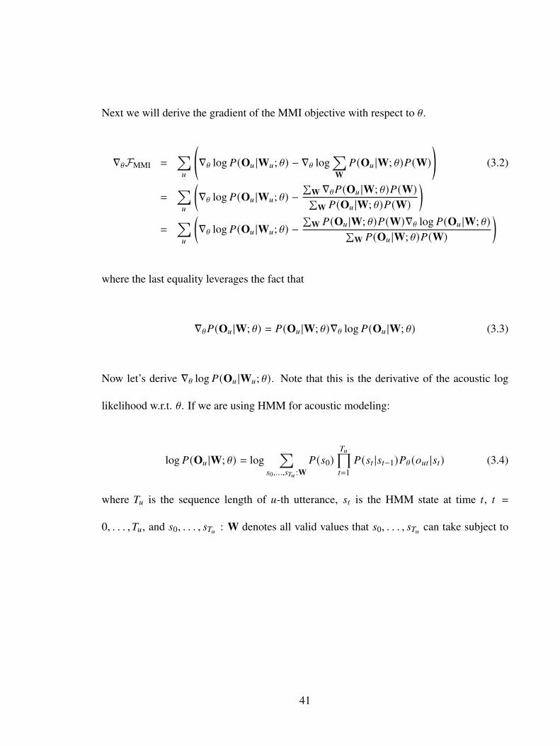
Next we will derive the gradient of the MMI objective with respect to \.
∇\FMMI =∑𝑢
(∇\ log 𝑃(O𝑢 |W𝑢; \) − ∇\ log
∑W𝑃(O𝑢 |W; \)𝑃(W)
)(3.2)
=∑𝑢
(∇\ log 𝑃(O𝑢 |W𝑢; \) −
∑W ∇\𝑃(O𝑢 |W; \)𝑃(W)∑
W 𝑃(O𝑢 |W; \)𝑃(W)
)=
∑𝑢
(∇\ log 𝑃(O𝑢 |W𝑢; \) −
∑W 𝑃(O𝑢 |W; \)𝑃(W)∇\ log 𝑃(O𝑢 |W; \)∑
W 𝑃(O𝑢 |W; \)𝑃(W)
)
where the last equality leverages the fact that
∇\𝑃(O𝑢 |W; \) = 𝑃(O𝑢 |W; \)∇\ log 𝑃(O𝑢 |W; \) (3.3)
Now let’s derive ∇\ log 𝑃(O𝑢 |W𝑢; \). Note that this is the derivative of the acoustic log
likelihood w.r.t. \. If we are using HMM for acoustic modeling:
log 𝑃(O𝑢 |W; \) = log∑
𝑠0,...,𝑠𝑇𝑢 :W𝑃(𝑠0)
𝑇𝑢∏𝑡=1
𝑃(𝑠𝑡 |𝑠𝑡−1)𝑃\ (𝑜𝑢𝑡 |𝑠𝑡) (3.4)
where 𝑇𝑢 is the sequence length of 𝑢-th utterance, 𝑠𝑡 is the HMM state at time 𝑡, 𝑡 =
0, . . . , 𝑇𝑢, and 𝑠0, . . . , 𝑠𝑇𝑢 : W denotes all valid values that 𝑠0, . . . , 𝑠𝑇𝑢 can take subject to
41

W and the HMM topology. Then
∇\ log 𝑃(O𝑢 |W; \) (3.5)
= ∇\ log∑
𝑠0,...,𝑠𝑇𝑢 :W𝑃(𝑠0)
𝑇𝑢∏𝑡=1
𝑃(𝑠𝑡 |𝑠𝑡−1)𝑃\ (𝑜𝑢𝑡 |𝑠𝑡)
=
∑𝑠0,...,𝑠𝑇𝑢 :W ∇\𝑃(𝑠0)
∏𝑇𝑢𝑡=1 𝑃(𝑠𝑡 |𝑠𝑡−1)𝑃\ (𝑜𝑢𝑡 |𝑠𝑡)∑
𝑠0,...,𝑠𝑇𝑢 :W 𝑃(𝑠0)∏𝑇𝑢𝑡=1 𝑃(𝑠𝑡 |𝑠𝑡−1)𝑃\ (𝑜𝑢𝑡 |𝑠𝑡)
=
∑𝑠0,...,𝑠𝑇𝑢 :W
∑𝑇𝑢𝑡=1 ∇\ log 𝑃(𝑜𝑢𝑡 |𝑠𝑡)𝑃(𝑠0)
∏𝑇𝑢𝑡=1 𝑃(𝑠𝑡 |𝑠𝑡−1)𝑃\ (𝑜𝑢𝑡 |𝑠𝑡)∑
𝑠0,...,𝑠𝑇𝑢 :W 𝑃(𝑠0)∏𝑇𝑢𝑡=1 𝑃(𝑠𝑡 |𝑠𝑡−1)𝑃\ (𝑜𝑢𝑡 |𝑠𝑡)
=
𝑇𝑢∑𝑡=1
∑𝑠0,...,𝑠𝑇𝑢 :W ∇\ log 𝑃(𝑜𝑢𝑡 |𝑠𝑡)𝑃(𝑠0)
∏𝑇𝑢𝑡=1 𝑃(𝑠𝑡 |𝑠𝑡−1)𝑃\ (𝑜𝑢𝑡 |𝑠𝑡)∑
𝑠0,...,𝑠𝑇𝑢 :W 𝑃(𝑠0)∏𝑇𝑢𝑡=1 𝑃(𝑠𝑡 |𝑠𝑡−1)𝑃\ (𝑜𝑢𝑡 |𝑠𝑡)
=
𝑇𝑢∑𝑡=1
∑𝑠𝑡 ∇\ log 𝑃(𝑜𝑢𝑡 |𝑠𝑡)
∑𝑠0,...,𝑠𝑡−1,𝑠𝑡+1,...,𝑠𝑇𝑢 𝑃(𝑠0)
∏𝑇𝑢𝑡=1 𝑃(𝑠𝑡 |𝑠𝑡−1)𝑃\ (𝑜𝑢𝑡 |𝑠𝑡)∑
𝑠0,...,𝑠𝑇𝑢 :W 𝑃(𝑠0)∏𝑇𝑢𝑡=1 𝑃(𝑠𝑡 |𝑠𝑡−1)𝑃\ (𝑜𝑢𝑡 |𝑠𝑡)
=
𝑇𝑢∑𝑡=1
∑𝑠𝑡 ∇\ log 𝑃(𝑜𝑢𝑡 |𝑠𝑡)𝑃(O𝑢, 𝑠𝑡 |W; \)
𝑃(O𝑢 |W; \)
=
𝑇𝑢∑𝑡=1
∑𝑠𝑡
∇\ log 𝑃(𝑜𝑢𝑡 |𝑠𝑡)𝑃(𝑠𝑡 |O𝑢,W; \)
The second equality is obtained by moving the derivative inside the log function and then
go on moving it inside the summation. The third equality is after applying product rule
for derivatives and making use of a similar trick as in Eq. (3.3). The fourth equality
is simply switching the summation in the numerator. The fifth equality is specifying a
particular order of the summing the sequence 𝑠0, . . . , 𝑠𝑇𝑢 . The sixth equality obtained by
marginalizing HMM states except 𝑠𝑡 . The last equality is from applying Bayes’ theorem.
42

If we plug Eq. (3.5) into Eq. (3.2), we have:
∇\FMMI (3.6)
=∑𝑢
𝑇𝑢∑𝑡=1
∑𝑠𝑡
∇\ log 𝑃(𝑜𝑢𝑡 |𝑠𝑡)(𝑃(𝑠𝑡 |O𝑢,W𝑢; \) −
∑W 𝑃(O𝑢 |W; \)𝑃(W)𝑃(𝑠𝑡 |O𝑢,W; \)∑
W 𝑃(O𝑢 |W; \)𝑃(W)
)=
∑𝑢
𝑇𝑢∑𝑡=1
∑𝑠𝑡
∇\ log 𝑃(𝑜𝑢𝑡 |𝑠𝑡)(𝑃(𝑠𝑡 |O𝑢,W𝑢; \) −
𝑃(𝑠𝑡 ,O𝑢; \)𝑃(O𝑢)
)=
∑𝑢
𝑇𝑢∑𝑡=1
∑𝑠𝑡
∇\ log 𝑃(𝑜𝑢𝑡 |𝑠𝑡) (𝑃(𝑠𝑡 |O𝑢,W𝑢; \) − 𝑃(𝑠𝑡 |O𝑢; \))
Now, log 𝑃(𝑜𝑢𝑡 |𝑠𝑡) is given by a neural network, so ∇\ log 𝑃(𝑜𝑢𝑡 |𝑠𝑡) is calculated by back-
propagation through the network. 𝑃(𝑠𝑡 |O𝑢,W𝑢; \) is the HMM state occupancy probability
conditioned on𝑊𝑢 and 𝑃(𝑠𝑡 |O𝑢; \) is the unconditional state occupancy probability. These
two quantities can be efficiently computed using the forward-backward algorithm over the
numerator graph and denominator graph respectively in Eq. (2.14). The numerator graph
is constrained by the reference W𝑢, meaning that all the paths in the graph correspond to
the reference transcript. Conceptually, the denominator graph is unconstrained with paths
and represents all possible sentences in a language. However, practically a subset of all
possible hypotheses, either in the form of a word lattice (in traditional MMI training) or
an n-gram phone language model (in LF-MMI) is used to approximate the sum over all
possible sentences. In either case, the denominator graph is actually constrained by a set
of sentences representing competing hypotheses against the reference transcript. “Lattice-
Free” in LF-MMI refers to the replacement of word lattices with an n-gram phone language
43

model, so that the probability tensor can fit into GPU memory for ASR. It also avoids the
need to generate such lattices by decoding the training data.
In either traditional MMI or LF-MMI, the numerator graph is acyclic, having exactly
the same number of time steps as that of the neural network’s output. The acyclic graph
is created from forced-alignments or decoding lattices with a prior trained model. For
example, in LF-MMI, an HMM-GMM tri-phone model, the same one used to generate
training labels in frame-level cross-entropy training, is used to generate lattices for numer-
ators. While it makes the training converge faster, it could potentially harm the flexibility
of learning alternative alignments if the HMM-GMM model is inaccurate in its alignments.
Also, having to train an additional model is not desirable as we always prefer simple but
still effective models.
Therefore we propose a wake word detection system with alignment-free LF-MMI as
training criterion, so as not to require such forced alignments for training. Alignment-
free LF-MMI was initially proposed for ASR [38]. In order to make it work for our task,
we made several necessary adaptations/changes to the lexicon, HMM topology, and data
preprocessing for both efficiency and performance reasons. A fast online decoder is also
proposed for the wake word detection task. Experiments on three real wake word data
sets all show its superior performance compared to the best of the other systems recently
reported in the literature.
44

3.2 Alignment-Free and Lattice-Free MMI
Training of Wake Word Detection Systems
3.2.1 HMM Topology
Different from other traditional HMM-based keyword-filler models (e.g., those pro-
posed in [15], [87], [117], [138] where each phoneme of the whole wake phrase corre-
sponds to an HMM or HMM state, we propose to model the whole wake phrase (in posi-
tive recordings) with a single HMM (referred to as word HMM), and the number of distinct
states within that HMM is a predefined value which is not necessarily proportional to the
number of phonemes in its pronunciation. We argue that using a fixed number of HMM
states, which is usually less than the number of the actual phonemes, has enough model-
ing power for the wake word task. Similarly, we use another HMM of the same topology
(referred to as freetext HMM) to model all non-silence speech (in negative audio exam-
ples). From our preliminary experiments we also found that having an additional HMM
dedicated to non-speech sounds, denoted SIL and called the silence HMM, is crucial for
good performance. SIL is added as optional silence [9] to the beginning and end of each
positive/negative recording so that it is exposed to at least some actual silence properly.
Note that in ASR, optional silence is also added between every pair of consecutive phones
in the lexicon (see Figure 3.1, where for a specific phone sequence DH IH1 S, it can either
follow the path 0 → 1 → 3 → 7 → 1, or 0 → 1 → 5 → 8 → 2 → 1. The latter one is
45

where optional silence is taking place.). If we make an analogy to ASR, optional silence
in our system is a special case of that as we only specify a single phone to each word. The
topologies we use are shown in Figure 3.2 and Figure 3.3.
0
1<eps>:<eps>
2
<eps>:<eps>
3DH:THIS
4W:WHY
5DH:THIS
6
W:WHY
SIL:<sil>
7IH1:<eps>
AY1:<eps>
8IH1:<eps>
AY1:<eps>
S:<eps>
S:<eps>
Figure 3.1: The illustration of a Lexicon FST with optional silence, which shows twoentries in the lexicon: DH IH1 S for the word THIS and W AY1 for the word WHY.input-symbol and output-symbol on arcs are represented as <input-symbol>:<output-symbol> and weights are omitted for clarity. Such representations apply to other WFSTfigures in this dissertation, if not otherwise specified.
46

0
0:0
11:1
0:0
22:0
0:0
33:0
0:0
44:0
Figure 3.2: The HMM topology used for the wake word and freetext. The number ofemitting HMM states is 4. The final state is non-emitting. We represent an HMM as aWFST. Note that here we use numbers, which are the indexes of symbols, to denote input-/output-symbols on arcs.
0
0:0
11:2
Figure 3.3: The HMM topology used for SIL. The number of emitting HMM states is 1.The final state is non-emitting.
3.2.2 Alignment-Free Lattice-Free MMI
In the regular LF-MMI the numerator graph used to compute the truth sequence is an
acyclic graph generated from frame-level alignments. In alignment-free LF-MMI [38],
the numerator graph is an unexpanded FST (usually with loops and self-loops) directly
47

0
1SIL
2SIL
3<word>
4<freetext>
5SIL
SIL
Figure 3.4: Topology of the phone language model FST for the denominator graph. Labelson arcs represent phones.
generated from training transcripts, giving more freedom to learn the alignments during
the forward-backward pass in training.
For ASR, the competing hypotheses in the denominator graph are constructed from a
phone LM trained from the training transcripts. By comparison, for the wake word detec-
tion task, we manually specify the topology of the phone LM FST as shown in Figure 3.4.
One path containing the word HMM corresponds to positive recordings, and the other two
correspond to negative recordings (other speech/non-speech and silence). If we have more
than one wake word as those in our Mobvoi (SLR87) data set, each wake word would cor-
respond to one such positive path. We assign final weights in a way such that they reflect
the ratio of the number of positive/negative examples in the training set.
48

3.2.3 Acoustic Modeling
Owing to efficiency and latency concerns specific to our task, the family of recurrent
[19], [46] or full-length self-attention-based [123] neural networks are not considered. In-
stead, we use a factorized time delay neural network (TDNN-F) architecture with skip
connections [95] for acoustic modeling. In a TDNN-F layer, the number of parameters
is reduced by factorizing the weight matrix in TDNN layers [91] into the product of two
low-rank matrices, the first of which is constrained to be semi-orthogonal. It is assumed
that the semi-orthogonal constraint helps to ensure that we do not lose information when
projecting from the high dimension to the low dimension.
The authors of the original paper found that, instead of factorizing the TDNN layer
into a convolution times a feed-forward layer, it is better to factorize the layer into two
convolutions with half the kernel size. For example, instead of using a kernel with context
(−3, 0, +3) in the first factor of the layer, and 0 context in the second factor, it is better to
use a kernel with context (−3, 0) in the first factor and a kernel with context (0, +3) in the
second factor. As we mentioned in Chapter 2, a larger kernel size/context means the output
needs to rely more input frames to compute a value, which incurs more latency in the wake
word detection. For example, an additional convolution layer with context (−3, 0, +3) will
add 6 more frames to the receptive field of the whole neural network.
As in architectures like ResNet [40], we incorporate skip connections. This means that
some layers receive input not only from the previous layer but also from other prior layers.
This allows us to make the network deeper by alleviating the vanishing gradient problem. In
49
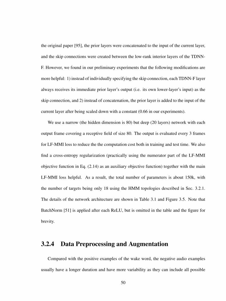
the original paper [95], the prior layers were concatenated to the input of the current layer,
and the skip connections were created between the low-rank interior layers of the TDNN-
F. However, we found in our preliminary experiments that the following modifications are
more helpful: 1) instead of individually specifying the skip connection, each TDNN-F layer
always receives its immediate prior layer’s output (i.e. its own lower-layer’s input) as the
skip connection, and 2) instead of concatenation, the prior layer is added to the input of the
current layer after being scaled down with a constant (0.66 in our experiments).
We use a narrow (the hidden dimension is 80) but deep (20 layers) network with each
output frame covering a receptive field of size 80. The output is evaluated every 3 frames
for LF-MMI loss to reduce the the computation cost both in training and test time. We also
find a cross-entropy regularization (practically using the numerator part of the LF-MMI
objective function in Eq. (2.14) as an auxiliary objective function) together with the main
LF-MMI loss helpful. As a result, the total number of parameters is about 150k, with
the number of targets being only 18 using the HMM topologies described in Sec. 3.2.1.
The details of the network architecture are shown in Table 3.1 and Figure 3.5. Note that
BatchNorm [51] is applied after each ReLU, but is omitted in the table and the figure for
brevity.
3.2.4 Data Preprocessing and Augmentation
Compared with the positive examples of the wake word, the negative audio examples
usually have a longer duration and have more variability as they can include all possible
50

Table 3.1: TDNN-F architecture for acoustic modeling in the wake word detection systems.
Layer Layer Type Contextfactor1
Contextfactor2
Skipconn.fromlayer
Size Innersize
1 TDNN-ReLU t-2, t+2 802 TDNN-F-ReLU t-1, t t, t+1 0 (input) 80 203 TDNN-F-ReLU t-1, t t, t+1 1 80 204 TDNN-F-ReLU t-1, t t, t+1 2 80 205 TDNN-F-ReLU t-1, t t, t+1 3 80 206 TDNN-F-ReLU t-1, t t, t+1 4 80 207 TDNN-F-ReLU t-1, t t, t+1 5 80 208 TDNN-F-ReLU t-1, t t, t+1 6 80 209 TDNN-F-ReLU t 7 80 2010 TDNN-F-ReLU t-3, t t, t+3 8 80 2011 TDNN-F-ReLU t-3, t t, t+3 9 80 2012 TDNN-F-ReLU t-3, t t, t+3 10 80 2013 TDNN-F-ReLU t-3, t t, t+3 11 80 2014 TDNN-F-ReLU t-3, t t, t+3 12 80 2015 TDNN-F-ReLU t-3, t t, t+3 13 80 2016 TDNN-F-ReLU t-3, t t, t+3 14 80 2017 TDNN-F-ReLU t-3, t t, t+3 15 80 2018 TDNN-F-ReLU t-3, t t, t+3 16 80 2019 TDNN-F-ReLU t-3, t t, t+3 17 80 2020 TDNN-F-ReLU t-3, t t, t+3 18 80 2018 Linear 3019 Dense-ReLU-Linear 30 8020 Dense N. targets
51

Figure 3.5: Schematic figure of our TDNN-F architecture corresponding to Table 3.1. Thenumber at the bottom-right corner of each TDNN-F block represents the number of repeatsof that block.
52
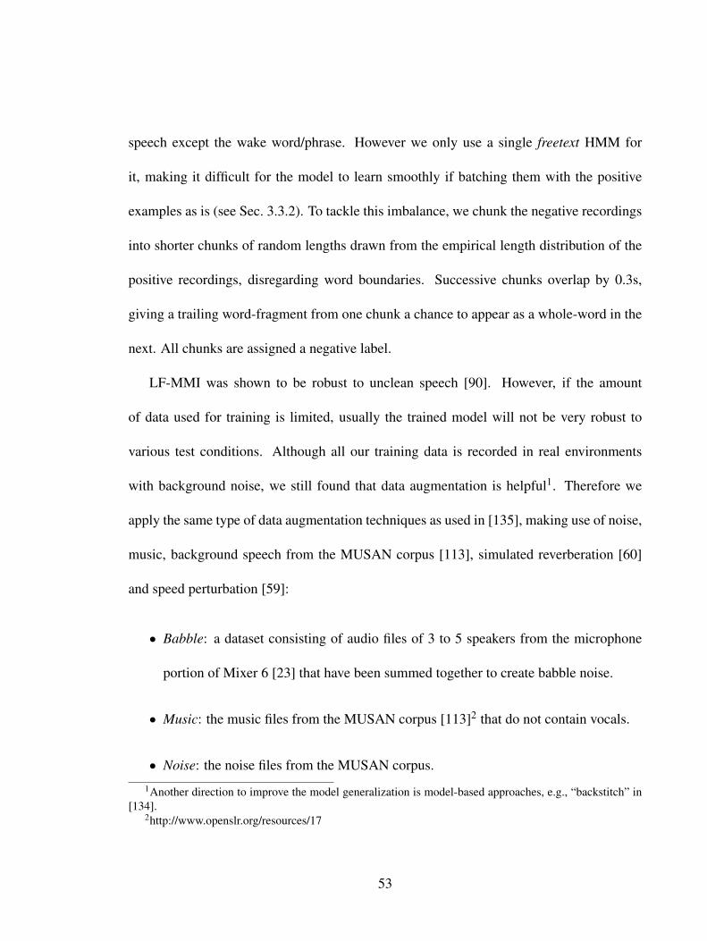
speech except the wake word/phrase. However we only use a single freetext HMM for
it, making it difficult for the model to learn smoothly if batching them with the positive
examples as is (see Sec. 3.3.2). To tackle this imbalance, we chunk the negative recordings
into shorter chunks of random lengths drawn from the empirical length distribution of the
positive recordings, disregarding word boundaries. Successive chunks overlap by 0.3s,
giving a trailing word-fragment from one chunk a chance to appear as a whole-word in the
next. All chunks are assigned a negative label.
LF-MMI was shown to be robust to unclean speech [90]. However, if the amount
of data used for training is limited, usually the trained model will not be very robust to
various test conditions. Although all our training data is recorded in real environments
with background noise, we still found that data augmentation is helpful1. Therefore we
apply the same type of data augmentation techniques as used in [135], making use of noise,
music, background speech from the MUSAN corpus [113], simulated reverberation [60]
and speed perturbation [59]:
• Babble: a dataset consisting of audio files of 3 to 5 speakers from the microphone
portion of Mixer 6 [23] that have been summed together to create babble noise.
• Music: the music files from the MUSAN corpus [113]2 that do not contain vocals.
• Noise: the noise files from the MUSAN corpus.
1Another direction to improve the model generalization is model-based approaches, e.g., “backstitch” in[134].
2http://www.openslr.org/resources/17
53
• Reverb: simulated RIRs3 as described in [60].
We randomly apply additive noises from the “babble”, “music” and “noise” datasets
separately on each copy of the original training audio. For each training example, “babble”
is added as background noises 3 to 7 times with SNRs ranging from 13 to 20; “music” is
added as background noises once with SNRs ranging from 5 to 15; “noise” is added as
foreground noises at the interval of 1 second with SNRs ranging from 0 to 15. Then re-
verberation is applied on top of them using the simulated RIRs with room sizes uniformly
sampled from 1 meter to 30 meters. The above procedure leads to 4 times more augmented
training data. The alignments for these augmented data, whenever needed (e.g. for compar-
ing to regular LF-MMI or frame-level cross-entropy models), are obtained from their clean
counterparts. In addition, we apply 3-fold speed perturbation [59] to the clean training data,
i.e., apply speed-perturbation with the factor of 1.1, 1.0 (original), and 0.9 respectively. In
total, these augmentations increase the amount of training data by 4 + 3 = 7-fold.
3.2.5 Decoding
We next describe online Viterbi decoding without lattice generation for wake word
detection, using the term “tokens” to denote partial hypotheses [85].
First we construct our decoding graph with a word-level FST specifying the prior prob-
abilities of all possible word paths, in a similar way as we specify the phone language
model FST in Figure 3.4, except that the start state and final states are merged to form a3http://www.openslr.org/resources/28
54

0
<sil>
1<sil>
2word
3
freetext
<sil>
<sil>
Figure 3.6: Topology of the word-level FST specifying the prior probabilities of all possibleword paths. Labels on arcs represent words.
loop. The loop allows decoding with an audio interleaving wake words with other possible
speech. As shown in Figure 3.6, the graph has one loop path <sil>→word→<sil> corre-
sponding to the positive segment, one loop path <sil>→freetext→<sil> corresponding to
the non-silence negative segment, and one self-loop path SIL corresponding to the pure
silence segment.
Algorithm 1 describes the online decoding procedure. It takes the prepared decoding
graph and the input audio stream as input and runs chunk-wise processing during online
decoding (starting from Line 4). A routine PROCESSEMITTINGANDNONEMITTING, ba-
sically doing Viterbi beam search, is invoked for every frame within the chunk, returning
surviving partial hypotheses as ACTIVETOKLIST (Line 9). Then depending on whether we
are processing the last chunk in the stream or not, we have different strategies:
55

Algorithm 1 Online Decoding for Wake Word DetectionInput: audioStream, graph ⊲ input stream and decoding graphOutput: isDetected ⊲ indicates whether the wake word is detected
1: procedure ONLINEDECODING(audioStream, graph)2: emitting← ∅3: isDetected← False4: for chunk in audioStream do5: activeTokList← ∅6: immortalTok← NULL7: prevImmortalTok← NULL8: for frame in chunk do9: activeTokList← ProcessEmittingAndNonEmitting(activeTokList, frame)
10: end for11: if chunk is the last one in audioStream then12: bestTok← BestToken(activeTokList)13: isDetected← BackTrack(bestTok, immortalTok)14: else15: (immortalTok, prevImmortalTok)←UpdateImmortalToken(activeTokList)
16: if immortalTok ≠ prevImmortalTok then17: isDetected← BackTrack(immortalTok, prevImmortalTok)18: if isDetected = True then19: break20: end if21: end if22: end if23: end for24: end procedure
56

• If it was not the last chunk, we update two consecutive “immortal tokens” IM-
MORTALTOKENS and PREVIMMORTALTOKENS in the routine UPDATEIMMORTAL-
TOKEN (Line 15), and backtrack along the frames delimited by these two tokens
4, checking whether there is a wake word detected from this partial backtracking
(Lines 16-19).
• If it was the last chunk, we take the best hypothesis from ACTIVETOKLIST as BEST-
TOK (in the routine BESTTOKEN) and backtrack from BESTTOK to IMMORTALTO-
KENS for the wake word (Lines 11-13).
In either case, once a wake word is found, stop decoding and trigger the system; other-
wise continue to process the next chunk if it exists.
What plays an essential role in Algorithm 1 is the “immortal tokens”. An “immor-
tal token” is the common ancestor (prefix) of all active tokens, i.e. it will not “die” no
matter which active token eventually survives. The way we compute and update “immor-
tal tokens” is described in the routine UPDATEIMMORTALTOKEN as Algorithm 2, where
Lines 3-8 obtain the last emitting token from each active token. Lines 12-28 find the com-
mon ancestor of all active tokens. Lines 30-32 update the immortal token (and assign the
old one to PREIMMORTALTOK) if a newer one is found; otherwise keep the old one from
the previous decoding step.
The intuition is that if all currently active partial hypotheses are from the same token at a
4These two consecutive tokens can refer to the same one, indicating no backtracking is needed at thatpoint.
57

Algorithm 2 Update the Immortal Token for BacktrackingInput: activeTokList ⊲ represents all current hypothesesOutput: immortalTok, prevImmortalTok ⊲ global, storing the latest one and previous
one respectively1: procedure UPDATEIMMORTALTOKEN(activeTokList)2: emitting← ∅3: for tok in activeTokList do4: while isNonEmittingToken(tok) do tok← tok.prev5: end while6: if tok ≠ NULL then emitting.insert(tok)7: end if8: end for9: prevImmortalTok← NULL
10: immortalTok← NULL11: tokenOne← NULL12: while True do13: if |emitting| = 1 then14: tokenOne← emitting[0]; break15: end if16: if emitting = ∅ then break17: end if18: prevEmitting← ∅19: for tok in emitting do20: prevTok← tok.prev21: while isNonEmittingToken(tok) do22: prevTok← tok.prev23: end while24: if prevTok = NULL then continue25: end if26: prevEmitting.insert(prevTok)27: end for28: emitting← prevEmitting29: end while30: if tokenOne ≠ NULL then31: prevImmortalTok← immortalTok32: immortalTok← tokenOne33: end if34: end procedure
58

previous time step, all hypotheses before that token had already collapsed to one hypothesis
(due to beam search pruning and token recombination), ), and there exists only one single
path between two immortal tokens, from which we would check whether it contains the
wake word in a chunk-by-chunk fashion. However, if the immortal token found at the end
of the current chunk is the same as the one found before, it means that any active tokens
have the risk of being pruned in the future, and we should wait until the next immortal
token appears for back-tracking, otherwise it is inefficient to track from every active token
back to the last immortal token.
3.3 Experiments and Analyses
3.3.1 Data Sets
There are three real wake word data sets available to us to conduct em-
pirical evaluations: the SNIPS data set (https://github.com/snipsco/
keyword-spotting-research-datasets) [24] with the wake word “Hey Snips”,
the Mobvoi single wake word data set5 [129] with the wake word “Hi Xiaowen”, and the
Mobvoi (SLR87) data set (https://www.openslr.org/87) [48] with two wake words
“Hi Xiaowen” and “Nihao Wenwen”. The statistics for each data set are summarized in
Table 3.2. We will use the first two data sets to demonstrate the effects of several design
choices in our system, and give the final results on all these three data sets when comparing
5This data set is not publicly available.
59

our system with others. If not otherwise specified, we show our experimental results in
an incremental way, meaning that later experiments would be conducted on top of the
one that is better from the previous experiment. The operating points in detection error
tradeoff (DET) [29] curves are obtained by varying the cost corresponding to the positive
path in the decoding graph while keeping the cost corresponding to negative path at 0.
40-dimensional MFCC features are extracted in all the experiments.
Table 3.2: Statistics for the three wake word data sets.
NameTrain Dev Eval
#Hrs #Utts (#Positive) #Hrs #Utts (#Positive) #Hrs #Utts (#Positive)
SNIPS 54 50,658 (5,799) 24 22,663 (2,484) 25 23,072 (2,529)Mobvoi 67 74,134 (19,684) 7 7,849 (2,343) 7 7,841 (1,942)
Mobvoi (SLR87) 144 174,592 (43,6256) 44 38,530 (7,357) 74 73,459 (21,282)
3.3.2 Effect of Negative Recordings Sub-segmentation
We first show the effect of sub-segmenting negative recordings on training. We start
from the training data with only speed-perturbation applied. To be consistent with the per-
formance reported by others on the same data sets, false rejection rate (FRR) is reported
in Table 3.3 at 0.5 false alarms per hour (FAH) on the SNIPS data set, and at 1.5 FAH
for Mobvoi. Apparently, without sub-segmentation the performance is far from satisfac-
tory. We also inspected the training/validation loss in both cases, and found that there is
severe overfitting when training without sub-segmentation: the gap between the training6 The statistics include two wake words.
60

Table 3.3: Effect of sub-segmentation of negative recordings.
FRR(%) SNIPS (FAH=0.5) Mobvoi (FAH=1.5)
w/o sub-segmentation 67 47w/ sub-segmentation 0.6 5.6
loss and the validation loss without sub-segmentation is much larger than that with sub-
segmentation (see Figure 3.7). This indicates that, given the correct labels, the LF-MMI
system is still unable to learn the forced-alignments for unsegmented examples well, i.e.,
poor generalization to the validation data.
61

0 20 40 60 80 100 120Iteration
0.07
0.06
0.05
0.04
0.03
0.02lo
g-pr
obab
ility
train with sub-segmentationvalid with sub-segmentationtrain without sub-segmentationvalid without sub-segmentation
log-probability plot for output
Figure 3.7: train/validation curves of LF-MMI objective: with v.s. without sub-segmentation of the negative training audios. Note that the numbers of total iterationsare different for the same number of epochs, because the total number of training examplesis changed after sub-segmentation.
3.3.3 Effect of Data Augmentation
We investigate the effect of data augmentation introduced in Section 3.2.4. The results
before and after augmentation are shown in Table 3.4. It can be seen that the augmentation
strategy is highly effective, where FRR with SNIPS is even 0 at FAH=0.5.
62

Table 3.4: Effect of data augmentation.
FRR(%) SNIPS (FAH=0.5) Mobvoi (FAH=1.5)
w/o data augmentation 0.6 5.6w/ data augmentation 0 0.4
3.3.4 Effect of Alignment-Free LF-MMI Loss
To compare our proposed alignment-free LF-MMI loss with regular LF-MMI and con-
ventional cross-entropy loss for our task, we train a phoneme-based HMM-GMM system
to generate the numerator lattice (for regular LF-MMI loss) or the forced alignments (for
conventional cross-entropy loss) for the same sub-segmented and augmented training data.
The network architectures are the same as that used for alignment-free LF-MMI training
except the final layer (depending on the loss being used).
The results in Table 3.5 validate that training with LF-MMI loss is generally advanta-
geous to training with frame-level cross-entropy loss in the wake word detection task, and
alignment-free LF-MMI loss achieves better performance than regular LF-MMI on SNIPS
and Mobvoi (SLR87), but worse on Mobvoi.
It is worth noting that we believe SNIPS and Mobvoi (SLR87) results are more in-
dicative of performance, as after manually listening to the false alarms in Mobvoi at this
specific operating point, we found that all the false alarms (9 in total) are actually inten-
tionally pronounced with a different tone on the last character “wen”, which is extremely
difficult for the model to learn given the limited amount of data; some would even argue that
63

those examples should be labeled as positive cases in order for the model to accommodate
Chinese speakers with accents. The better performance of the system with alignment-free
LF-MMI loss is possibly due to the capability of learning more flexible alignments than
GMM models.
Table 3.5: Effect of alignment-free LF-MMI loss.
FRR(%)SNIPS (FAH=0.5) Mobvoi (FAH=1.5) Mobvoi (SLR87) (FAH=0.5)
Hi Xiaowen Nihao Wenwen
cross-entropy 0.6 3.5 1.7 2.5regular LF-MMI 0.1 0.2 0.6 0.7alignment-free LF-MMI 0 0.4 0.4 0.5
3.3.5 Regular LF-MMI Refinement
The experiment from the previous section motivates us to do an additional experi-
ment investigating how the regular LF-MMI performs when it gets alignments from the
alignment-free LF-MMI system instead of from a GMM model, and whether the regular
LF-MMI training could further improve the performance as a refinement of our existing
system. To this end, we compare the three systems in Table 3.6. Note that as we already
achieve FRR=0 at FAH=0.5 with SNIPS using our alignment-free LF-MMI system, we
set the operating point at a smaller FAH (0.04) for it. Table 3.6 demonstrates that further
improvement can be obtained by running an additional regular LF-MMI training on top of
alignment-free LF-MMI, suggesting an optional refinement stage for better performance.
64

Table 3.6: Effect of using alignments from Alignment-free LF-MMI for regular LF-MMI.
FRR(%)SNIPS (FAH=0.04) Mobvoi (FAH=1.5) Mobvoi (SLR87) (FAH=0.5)
Hi Xiaowen Nihao Wenwen
regular LF-MMI 0.2 0.2 0.6 0.7alignment-free LF-MMI 0.2 0.4 0.4 0.5
+regular LF-MMI refinement 0.1 0.3 0.4 0.4
3.3.6 Comparison with Other Baseline Systems
We compare our proposed system with other systems recently proposed for the same
data sets. We use our alignment-free LF-MMI system without refinement, as the refinement
is optional. The results are shown in Table 3.7. DET curves of our system on all the three
data sets are plotted in Figure 3.8.
For the SNIPS data set we compare against their original paper [24], where a voice
activity detection system is used to obtain frame-level wake word labels for training. While
their system is already very good in term of FRR, our system even achieves FRR=0 at
FAH=0.5.
For the Mobvoi data set we compare our system with [129] where an attention mech-
anism is adopted for pooling across frames to make a prediction. They also propose
an adversarial examples generation algorithm for robust training. The modeling units
are wake words, and they use recurrent rather than convolutional networks. Our system
achieves significantly better results, improving FRR to 0.4%, compared to their FRR=3.6%
at FAH=1.5, a 90% relative reduction.
For the Mobvoi (SLR87) data set, the approach proposed in [49] is compared, where
65

the label imbalance issue is tackled by selective negative sampling. Again, it uses wake
words as modeling units. Note that this data set contains two wake words (“Hi Xiaowen”
and “Nihao Wenwen”), and when we are evaluating for a specific one, the other one is con-
sidered a false alarm or negative example. We achieve 50-70% reduction in FRR compared
to their system at the same FAH=0.5.
Table 3.7: Comparison with other wake-word detection baselines.
SNIPS #Params FRR(%) at FAH=0.5Coucke at al. [24] 220k 0.12alignment-free LF-MMI (Ours) 150k 0
Mobvoi #Params FRR(%) at FAH=1.5Wang at al. [129] 84k ∼3.6alignment-free LF-MMI (Ours) 150k 0.4
Mobvoi (SLR87) #ParamsFRR(%) at FAH=0.5
Hi Xiaowen Nihao WenwenHou at al. [49] 7 N/A 1.3 1.0alignment-free LF-MMI (Ours) 150k 0.4 0.5
7 The numbers shown here, different from those in the original paper, are obtained at https://github.com/jingyonghou/KWS_Max-pooling_RHE on the same data as what we are using.Those shown in theoriginal paper are obtained from an in-house dataset.
66

0.00 0.25 0.50 0.75 1.00 1.25 1.50 1.75 2.00False Alarms per hour
0.0
0.2
0.4
0.6
0.8
1.0
1.2
1.4
1.6
False
Rej
ectio
n Ra
te (%
)SNIPSMobvoiMobvoi (SLR87) 'Hi Xiaowen'Mobvoi (SLR87) 'Nihao Wenwen'
DET curve
Figure 3.8: DET curves for the three data sets.
3.3.7 Different Model Sizes and Receptive Field
Since we already achieve good performance with the current wake word detection sys-
tem, we would like to further reduce the neural network size, as well as the the size of the
receptive field, to a a smaller memory footprint for the model and low detection latency
respectively. Some recent work [4], [150] shows that neural networks with size of 20-100k
can already have competitive performance in the KWS task. We gradually reduce the model
size of the LF-MMI model by removing some layers, to investigate how the performance
67

Table 3.8: Results of reducing model size and receptive field for alignment-free LF-MMIon SNIPS.
Model Size #layers receptive field FRR(%) at FAH=0.5
149k 20 87 0143k 19 81 0.1136k 18 75 0.2123k 16 63 0.4110k 14 51 0.597k 12 47 0.491k 11 41 0.478k 9 37 0.7
is affected. Note that when removing layers, the receptive field of each output frame is
potentially getting smaller, depending on the layer removed.
Table 3.8 shows the results when reducing the model size in our proposed alignment-
free LF-MMI model. We can see that when the receptive field becomes smaller as result
of reducing the number of layers, the performance tends to degrade. When the receptive
field is 41, it can still achieve FRR=0.4% at FAH=0.5. However, when the receptive field
is further reduced to 37 (at which the model size is 78k), there is a significant loss in FRR.
Table 3.9 is the results of the same experiment conducted on Mobvoi (SLR87). Overall
it shows a similar trend as in SNIPS. The point of significant degradation happens when
the receptive field is reduced from 75 to 63, suggesting 70 is necessary to maintain good
performance.
68

Table 3.9: Results of reducing model size and receptive field for alignment-free LF-MMIon Mobvoi (SLR87).
Model Size #layers receptive field FRR(%) at FAH=0.5
Hi Xiaowen Nihao Wenwen
150k 20 87 0.4 0.5143k 19 81 0.4 0.6137k 18 75 0.5 0.7124k 16 63 0.6 1.2111k 14 51 1.0 1.398k 12 47 1.1 1.391k 11 41 2.0 2.6
3.3.8 Alignment Analysis
The superior detection performance of the alignment-free LF-MMI system over regular
LF-MMI motivates us to examine their state-level alignments for better understanding their
difference. We also would like to know, given the 4-state HMM, how often each state
appears in these alignments. We first choose the Mobvoi (SLR87) dataset for analysis as
it has the largest training set (144 hours) among the three. As there are no ground truth
alignments, we have to analyze them qualitatively.
We look at the forced-alignments generated from 3 types of the acoustic model: 1)
the GMM model used in the regular LF-MMI providing the numerator supervision for
LF-MMI; 2) the neural network trained with regular LF-MMI; and 3) the neural network
trained from scratch (alignment-free LF-MMI).
For both positive and negative examples, the state-level alignments generated from the
GMM model are much more diverse than those from the LF-MMI trained neural networks,
69

meaning more states within an HMM are occupied by quite a few number of frames. It can
be explained by the fact that LF-MMI is a kind of sequence-level loss optimizing sequence
posteriors and it does not focus on frame-level alignments. On the other hand, GMM
is trained with HMM generatively maximizing the likelihood of the data, and generative
models tend to be in favor of more complicated models. Therefore the generatively trained
HMM-GMM will achieve better data likelihood if more HMM states get involved.
Now let’s look at the examples in groups. For positive examples (i.e. containing “HiXi-
aowen” or “NihaoWenwen”), around 60% of these examples have leading or trailing silence
lasting at least 10% of the total duration in their alignments from the GMM model, while
from the other two models there is almost no silence. After listening to the original audio, it
turns out that the part aligned to silence from the GMM models is mostly not pure silence,
but rather non-speech background white noise (see Figure 3.9a). Actually there are very
few frames corresponding to pure silence. For negative examples, the GMM model often
mistakenly aligns the beginning or ending part of non-wake-word speech frames to silence,
while the other two models rarely align frames to silence. We found, after listening to those
negative examples, that there is nearly no noticeable leading or trailing silence (See Fig-
ure 3.10a). In sum, neither positive nor negative examples have enough leading or trailing
silence in the Mobvoi (SLR87) dataset, making it difficult to learn a reliable silence model.
We note that the SNIPS dataset contains more positive and negative examples with si-
lence at the beginning or end (See Figure 3.9b for the positive and Figure 3.10b for the
negative). So we carried out the same analysis on SNIPS. The phenomenon that one state
70

dominates among others in an HMM for LF-MMI trained models still exists in both pos-
itive and negative examples. On the other hand, the word-level alignment patterns are
different from those for Mobvoi (SLR87). The GMM model has a tendency of aligning
quite a large number of frames, either at the beginning or ending of an example, to silence,
for both positive and negative examples. The regular LF-MMI can mostly align silence
frames correctly, and usually makes mistakes when trying to align very short silence at the
beginning or end. However, the alignment-free LF-MMI model is still not able to align the
silence frames well: at most only the first frame is aligned to silence. It can be attributed
to the freedom of learning alignments that alignment-free LF-MMI has, as it does not pay
attention to individual frames, despite its best overall detection performance. Note that no
silence in an alignment does not imply the probability of silence is 0; it just means that the
posterior probability of silence is not higher than that of wake words and non-silence. Fig-
ure 3.11 shows the neural network output over time from a positive example of the SNIPS
dataset. Each curve corresponds to log probability of the acoustics given a specific state
over time i.e., log 𝑃(𝑜𝑢𝑡 |𝑠𝑡) for 𝑡 ∈ 1, . . . , 𝑇, and curves with the state belonging to the
same HMM have the same color. For example, the SIL HMM has two states, and the curves
for these two states are colored with red. The values on these two red curves are around 0
in most of the time, meaning that their probability mass is far above 0 (if the probability is
close to 0, then the log probability is a negative value far from 0).
71

0 5000 10000 15000 20000
0.75
0.50
0.25
0.00
0.25
0.50
0.75
(a) The waveform of a typical positive example from Mobvoi (SLR87).
0 5000 10000 15000 20000 25000 30000 35000
0.4
0.2
0.0
0.2
0.4
0.6
(b) The waveform of a typical positive example from SNIPS.
Figure 3.9: Examples of positive waveforms from two datasets to illustrate their differencein silence at the beginning/end. There is tiny wave before/after the wake word in the topsubfigure indicating background noise, while in the bottom one it is more “silent” in thecorresponding regions.
72

0 20000 40000 60000 80000
0.75
0.50
0.25
0.00
0.25
0.50
0.75
(a) The waveform of a typical negative example from Mobvoi (SLR87).
0 20000 40000 60000 80000 100000 120000 140000 160000
0.100
0.075
0.050
0.025
0.000
0.025
0.050
0.075
(b) The waveform of a typical negative example from SNIPS.
Figure 3.10: Examples of negative waveforms from the two datasets to illustrate their dif-ference in silence at the beginning/end. Compared with the top subfigure, the bottom onehas a more significant portion of silence at the beginning.
73

0 10 20 30 40 50 60 70frame
7.5
5.0
2.5
0.0
2.5
5.0
7.5
10.0
log-
prob
SILheysnipsfreetext
log-prob curves for pdf-ids.
Figure 3.11: The neural network output over time from a positive example of the SNIPSdataset.The x-axis is for frames and y-axis represents the log-probability of the acousticfeatures given an HMM state. Each curve corresponds to a specific HMM state. Curveswith the state from the same HMM have the same color.
3.3.9 One-state experiments
In Section 3.3.8 we found that when generating forced alignments with an LF-MMI
trained model, one state usually dominates over the other emitting states belonging to the
same HMM. A natural question arises: now that the other states are mostly not used, what
if we further simplify the HMM topology. Recall that in Section 3.2.1 we specified the
topologies for the wake word HMM and freetext HMM as 4 emitting states followed by 1
74
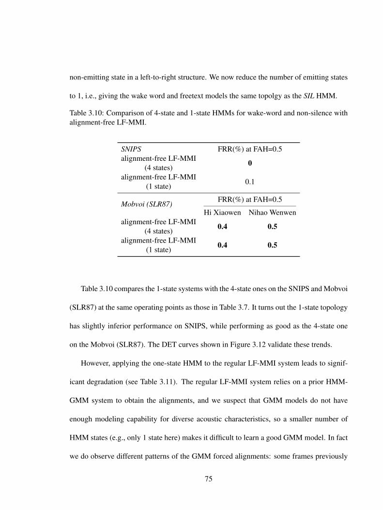
non-emitting state in a left-to-right structure. We now reduce the number of emitting states
to 1, i.e., giving the wake word and freetext models the same topolgy as the SIL HMM.
Table 3.10: Comparison of 4-state and 1-state HMMs for wake-word and non-silence withalignment-free LF-MMI.
SNIPS FRR(%) at FAH=0.5alignment-free LF-MMI
(4 states) 0
alignment-free LF-MMI(1 state) 0.1
Mobvoi (SLR87)FRR(%) at FAH=0.5
Hi Xiaowen Nihao Wenwenalignment-free LF-MMI
(4 states) 0.4 0.5
alignment-free LF-MMI(1 state) 0.4 0.5
Table 3.10 compares the 1-state systems with the 4-state ones on the SNIPS and Mobvoi
(SLR87) at the same operating points as those in Table 3.7. It turns out the 1-state topology
has slightly inferior performance on SNIPS, while performing as good as the 4-state one
on the Mobvoi (SLR87). The DET curves shown in Figure 3.12 validate these trends.
However, applying the one-state HMM to the regular LF-MMI system leads to signif-
icant degradation (see Table 3.11). The regular LF-MMI system relies on a prior HMM-
GMM system to obtain the alignments, and we suspect that GMM models do not have
enough modeling capability for diverse acoustic characteristics, so a smaller number of
HMM states (e.g., only 1 state here) makes it difficult to learn a good GMM model. In fact
we do observe different patterns of the GMM forced alignments: some frames previously
75

0.00 0.25 0.50 0.75 1.00 1.25 1.50 1.75 2.00False Alarms per hour
0.0
0.2
0.4
0.6
0.8
1.0
1.2
1.4
1.6
False
Rej
ectio
n Ra
te (%
)
4-state 'Hi Xiaowen'4-state 'Nihao Wenwen'4-state 'Hey Snips'1-state 'Hi Xiaowen'1-state 'Nihao Wenwen'1-state 'Hey Snips'
DET curve
Figure 3.12: DET curves: 4-state v.s. 1-state with alignment-free LF-MMI. All red curvesare with 4 states and all blue curves are with 1 state. Different line styles correspond todetecting different wake words.
76

aligned to the wake word or non-silence in the 4-state system are now aligned to silence in
the 1-state system.
Experiments in this section suggest another advantage of alignment-free LF-MMI: it
requires a smaller number of HMM states to achieve good detection performance. We still
would like to keep the 4-state HMM in the proposed version as it achieves the best detection
performance across different datasets and is more resistant to misalignments.
Table 3.11: Comparison of 4-state and 1-state HMMs for wake-word and non-silence withregular LF-MMI.
SNIPS FRR(%) at FAH=0.5regular LF-MMI
(4 states) 0.1
regular LF-MMI(1 state) 2.3
Mobvoi (SLR87)FRR(%) at FAH=0.5
Hi Xiaowen Nihao Wenwenregulare LF-MMI
(4 states) 0.6 0.7
regular LF-MMI(1 state) 1.0 1.0
3.3.10 Decoding Analysis
In this section we examine the performance of the proposed decoding algorithm intro-
duced in Section 3.2.5 used for wake word detection. The task of wake word detection
requires low detection latency, i.e., the system should be triggered as soon as the wake
word appears in the audio stream, while still maintaining high detection accuracy. There
77

are basically two factors affecting the detection latency. One is the receptive field of the
neural network which determines the number of future frames to look at in order to com-
pute the output at a frame. This has been discussed in Section 3.3.7 where we observe that
there is no significant degradation unless the receptive field is below 40/70 frames (or the
number of dependent future frames is smaller than 20/35) for SNIPS and Mobvoi (SLR87)
respectively. The other factor is the delay of being triggered by a detected word, which
is normally measured by the difference between the triggered time and the time when the
wake word ends. Unfortunately, none of the datasets we are using has the ground-truth
timing information of wake words, which prevent us from providing accurate and quanti-
tative analysis of the latency. We instead provide some qualitative and indirect analysis,
by showing visualized examples, providing some statistics during decoding, and observing
performance changes with different level of decoding constraints.
Recall that the immortal tokens introduced in Algorithm 2 play the role of notifying
the decoder to back-track between two consecutive immortal tokens, checking if a wake
word exists in the hypothesis. There are two possible cases when we do the back-tracking
and then detect a wake word: 1) the last immortal token is identified before the decoder
reaches the end of the audio recording, and the wake word is detected when back-tracking
from that immortal token to the previous one; and 2) the wake word is not detected until
the decoder reaches the end of the recording, and the best one among all the surviving
tokens is selected for back-tracking in which the wake word is detected. Clearly the second
case is less preferable, as it suggests potential delays during the detection. In order to
78
know how many times the wake word is detected in each of these two cases, we count
them on both SNIPS and Mobvoi (SLR87), each with cross-entropy, regular MMI and
alignment-free MMI trained models. We set the frequency of checking the immortal token
to every 1 frame by making the chunk size in Algorithm 1 equal to 1, so that there is no
extra delay introduced by the chunk size itself. For convenience we perform the counting at
FAH=0.5 in each experiment, although empirically there is not much difference if obtaining
the counts at other operating points nearby.
Table 3.12 shows the statistics, from which we have two observations:
• The alignment-free LF-MMI has more cases when the back-tracking happens at the
end of the utterance than regular LF-MMI and cross-entropy systems. The reason,
we believe, is that the alignment-free LF-MMI tends to learn delayed alignments for
achieving a better training criterion.
• The “back-tracking at the end” case happens more frequently for the alignment-free
LF-MMI on Mobvoi (SLR87) than on SNIPS. In Section 3.3.8 we mentioned that
the positive examples in SNIPS usually contain leading/trailing silence, while Mob-
voi (SLR 87) has much less such cases. The occurrence of “back-tracking at the end”,
however, does not necessarily imply large detection latency if there is not much trail-
ing silence (as is the case for Mobvoi (SLR 87)); in that case the recording just ends
right after the wake word ends.
Due to lack of ground-truth timing information, we instead show some qualitative ex-
79

Table 3.12: The percentage (%) of all positives in the Eval set that are triggered beforereaching the end of examples.
System TypeSNIPS (FAH=0.5) Mobvoi (SLR87) (FAH=0.5)
Hi Xiaowen Nihao Wenwen
cross-entropy 97.8 99.2 99.2regular LF-MMI 95.3 92.3 97.3alignment-free LF-MMI 62.1 37.3 35.5
amples for detection latency. Figure 3.13 shows three examples on SNIPS. Each example
is a waveform with two epochs marked by vertical lines: the black line indicates the frame
at which the detector triggers, and the red vertical lines indicate the time when the latest
immortal token is generated before the detector triggers. The x-axis represents the speech
sample index. Fig 3.13a shows an example with a long duration of trailing silence. The last
immortal token is identified at the time when “Hey Snips” just finished, and the triggered
time is about 0.2 second later (the sampling rate is 16k). Fig 3.13b shows an example with
long leading silence but short trailing silence, in which the triggered time is also around 0.2
second after the end of the wake word. Fig 3.13c gives an example where the last immortal
token is identified within the segment corresponding to the wake word, and the triggered
time is about 0.4 second later after the wake word.
Figure 3.14 shows 3 examples on Mobvoi (SLR87), which is much more noisy than
SNIPS. Figure 3.14a is a case where there is a lot of background noise during and after
the wake word “Hi Xiaowen”. The “bottleneck” between the red and black line is actually
the end of the wake word, so the delay of the triggered time is around 0.5 second. Figure
80

3.14b demonstrates another example where there is a long trailing “silence” (with some
mild noise) and it looks like the system is triggered on time. In Figure 3.14c we show an
example where it is triggered at the end and there is no immortal token identified (so the red
line is placed at the first frame), which means that there is no such a point when multiple
hypotheses have ever collapsed to a single hypothesis during the decoding.
To further investigate the latency, we conduct two more experiments: we restrict the
the maximum number of back-tracking steps starting from 1) the current immortal token
towards the previous immortal token at line 17 in Algorithm 1, or 2) the best surviving
token at the last frame if it is reached at line 13. We apply these two constraints separately
so that we would know their individual influences on performance. It turns out that the
former constraint does not have significant impact on the detection results for either the
regular or the alignment-free LF-MMI system even with a small maximum number (i.e.,
20 frames), implying there are no much delay in triggering wake words within the time
interval between the current and previous immortal token.
However, the latter constraint has significant impact if the maximum number of back-
tracking frames is getting smaller. The details are shown in Table 3.13 8. For both regular
and alignment-free LF-MMI, the detection performance degrades significantly when the
maximum number of back-tracking frames is small, i.e. when maximum number of back-
tracking frames is below 50 for regular LF-MMI, or below 80 for alignment-free MMI.
Also we can observe that regular LF-MMI is more robust to smaller number of back-
8∞ means not applying any constraint for max. back-tracking #frames.
81

0 10000 20000 30000 40000 50000 60000 70000 80000
0.4
0.2
0.0
0.2
0.4
(a) An example with a long duration of trailing silence.
0 20000 40000 60000 80000 100000 120000
1.00
0.75
0.50
0.25
0.00
0.25
0.50
0.75
(b) An example with a long duration of leading silence.
Figure 3.13: Positive examples showing the detection latency on SNIPS. The black verticallines indicate triggered time, and the red vertical lines indicate the time when the latestimmortal token is generated before the triggered time.
82

0 5000 10000 15000 20000 25000 30000
0.4
0.2
0.0
0.2
0.4
0.6
0.8
(c) An example where the the time when the system is triggered is abit late.
tracking frames than the alignment-free one when backtracking from the last frame, which
provides another evidence that the alignment-free LF-MMI trained system leads to a more
delayed triggering.
Motivated by the observations above, we slightly modify Algorithm 1 and 2, such that
we maintain a variable last_checked_frame storing the last frame from which we re-
cently back-tracked. last_checked_frame is updated whenever a new immortal token
is identified, or a forced back-tracking is invoked. If the frame being reached by the de-
coder is at least 𝑁 frames ahead from last_checked_frame, back-tracking is forced to
be invoked from the best token at that frame. So 𝑁 gives an upper bound of how often the
decoder checks for the wake word. We initially set 𝑁 to a small value (e.g., 30), and then
gradually increase it while monitoring the changes of the detection results. As expected,
83
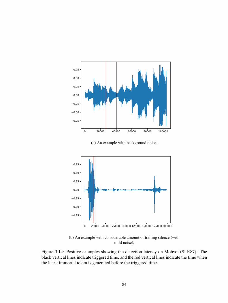
0 20000 40000 60000 80000 100000
0.75
0.50
0.25
0.00
0.25
0.50
0.75
(a) An example with background noise.
0 25000 50000 75000 100000 125000 150000 175000 200000
0.75
0.50
0.25
0.00
0.25
0.50
0.75
(b) An example with considerable amount of trailing silence (withmild noise).
Figure 3.14: Positive examples showing the detection latency on Mobvoi (SLR87). Theblack vertical lines indicate triggered time, and the red vertical lines indicate the time whenthe latest immortal token is generated before the triggered time.
84

0 5000 10000 15000 20000 25000
0.75
0.50
0.25
0.00
0.25
0.50
0.75
(c) An example with few trailing silence
Table 3.13: Performance comparison with varying the number of max back-tracking framesfrom the end of examples.
System TypeMax. back-tracking #frames
Mobvoi (SLR87) (FAH=0.5)
Hi Xiaowen Nihao Wenwen
regular LF-MMI
∞ 0.6 0.7120 0.6 0.7100 0.6 0.780 0.8 0.750 0.8 1.630 18.0 5.9
aligment-free LF-MMI
∞ 0.4 0.5140 0.4 0.5120 0.5 0.6100 0.7 0.980 2.0 3.050 61.1 58.7
85

the results keep improving before reaching a plateau. 𝑁 at which the plateau starts is about
40 for regular LF-MMI, and about 80 for alignment-free LF-MMI. This experiment also
provides a rough and indirect estimate of latency.
In sum, the alignment-free LF-MMI system has larger detection latency than the regular
LF-MMI system. To control the latency, we can leverage the modified algorithm introduced
in the previous paragraph and specify a value for 𝑁: a smaller 𝑁 leads to low latency but
may hurt the detection performance.
3.3.11 Resources Consumption
As wake word detection systems usually run on devices where there are very limited
computation and memory resources, it is useful to provide some measures of computation
and memory resources consumption during the detection stage for reference.
The first one is the number of floating point operations. It measures how much compu-
tation is needed to evaluate a model. The more floating point operations, the more power
consumption. Here we calculate the number of floating point operations in the neural net-
work 9. For example, the matrix multiplication A × B, where A ∈ R𝑚×𝑘 and B ∈ R𝑘×𝑛,
involves 2𝑚𝑛𝑘 floating point operations (𝑚𝑛𝑘 arithmetic additions and 𝑚𝑛𝑘 arithmetic
multiplications). In a convolution, the kernel matrix is repeatedly applied on patches of
9The computation in the decoder in negligible compared to that in the neural network.
86

input. Taking 1D convolution for instance, the number of repeats is computed as:
num_repeats =⌊𝐿 + 2 × padding − dilation × (kernel_size − 1) − 1
stride+ 1
⌋(3.7)
where 𝐿 is the input length. Based on the neural architecture specified in Table 3.1, the
number of floating point operations is about 292, 000 × 𝑇 where 𝑇 is the number of input
feature frames.
The second one is the peak memory usage. We use the Linux command:
ps -o rss= $pid
where $pid is the process id of the running decoding program, to obtain resident set size
(RSS) 10. The decoding is run on an Intel Xeon CPU E5-2620 v3 @ 2.40GHz. The max-
imum value of RSS during the execution of the program is recorded as the peak value. It
turns out that the peak memory usage is 77 MB. Note that we run the decoding purely on
CPUs, so both the executions of neural network’s forward pass and the online decoding are
on CPUs.
3.3.12 Unsuccessful Experiments
There are several other design choices we have tried before arriving at the system pro-
posed in Section 3.2. Those choices turned out to be unsuccessful, so we discarded them or
found other alternatives in our final system. However, we think some of those are valuable
10 RSS is the portion of memory occupied by a process that is held in main memory (RAM) [101].
87

for discussions. In this section, we give our initial motivation of those attempts, along with
the experiments and analyses for these negative results.
3.3.12.1 Two-HMM Experiments
There are 3 HMMs in our final system: word, freetext and SIL corresponding to 3 dis-
tinct classes of pronunciation units11 to be learned. Note that our annotations only contain
two labels: either positive or negative (including non-silence and silence) for training. The
problem is mainly for negative examples: it is possible that a negative example contains
non-silence and silence interleaving with each other. Consider the an example where the
underlying transcript is like:
[silence] [non-silence] [silence] [non-silence] [silence]
where “[non-silence]” represents any non-silence text except the wake word and “[silence]”
is the silence. However the supervision for this example is a single label representing
negative. While the leading and trailing silence can be captured by optional silence added
to the lexicon FST [9], silence in the middle of non-silence will not. So conceptually
the setup in the proposed system cannot follow arbitrary combinations of non-silence and
silence.
Therefore, our attempt was to merge freetext and SIL as a single “negative HMM”
without differentiating between non-silence and silence at the whole word level, and in-
stead relying on the underlying HMM topology to account for it. One possible way is to11In ASR pronunciation units are usually phones. But in our wake word detection system, we use a single
HMM to model the wake word, silence, or other non-silence text, so actually the pronunciation units aremodeling acoustics longer than phones.
88

have an HMM topology with two emitting states having an arc to each other (i.e. ergodic),
where one state corresponds to non-silence and the other state corresponds to silence (Fig-
ure 3.15). A more complicated way is to have more than 2 states for the negative HMM,
having an arc from the last emitting state to the first emitting state to account for interleav-
ing between non-silence and silence (E.g., in Figure 3.16 we have 1-state for silence and 4
states for non-silence).
0
0:0
11:0
24:13:0
0:0
2:1
Figure 3.15: A negative HMM topology with 2 emitting states, each of which has an arc tothe other. State 0 and 1 also have an arc to the final non-emitting state.
89
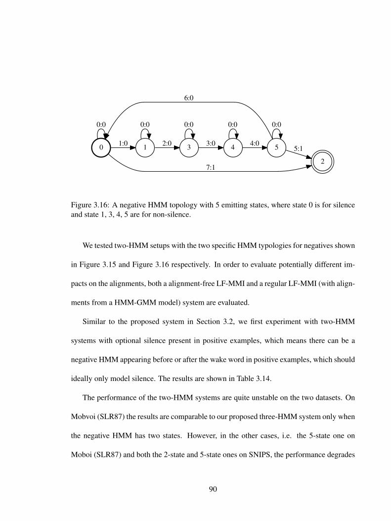
0
0:0
11:0
27:1
0:0
32:0
0:0
43:0
0:0
54:0
6:0
5:1
0:0
Figure 3.16: A negative HMM topology with 5 emitting states, where state 0 is for silenceand state 1, 3, 4, 5 are for non-silence.
We tested two-HMM setups with the two specific HMM typologies for negatives shown
in Figure 3.15 and Figure 3.16 respectively. In order to evaluate potentially different im-
pacts on the alignments, both a alignment-free LF-MMI and a regular LF-MMI (with align-
ments from a HMM-GMM model) system are evaluated.
Similar to the proposed system in Section 3.2, we first experiment with two-HMM
systems with optional silence present in positive examples, which means there can be a
negative HMM appearing before or after the wake word in positive examples, which should
ideally only model silence. The results are shown in Table 3.14.
The performance of the two-HMM systems are quite unstable on the two datasets. On
Mobvoi (SLR87) the results are comparable to our proposed three-HMM system only when
the negative HMM has two states. However, in the other cases, i.e. the 5-state one on
Moboi (SLR87) and both the 2-state and 5-state ones on SNIPS, the performance degrades
90

Table 3.14: Comparisons of three-HMM and two-HMM alignment-free LF-MMI systems(with optional silence).
SystemFRR(%) at FAH=0.5
SNIPS Mobvoi (SLR 87)Hi Xiaowen Nihao Wenwen
3 HMMs (proposed) 0 0.4 0.52 HMMs
(2 states for negatives) 99.8 0.5 0.5
2 HMMs(5 states for negatives) 26.9 74.0 50.2
Table 3.15: Comparisons of three-HMM and two-HMM regular LF-MMI systems (withoptional silence).
SystemFRR(%) at FAH=0.5
SNIPS Mobvoi (SLR 87)Hi Xiaowen Nihao Wenwen
3 HMMs 0.1 0.6 0.72 HMMs
(2 states for negatives) 0.5 0.6 0.7
2 HMMs(5 states for negatives) 14.9 0.5 0.7
91

so drastically that quite a large amount of positive examples are missing in the detection.
Recall that in Section 3.3.9 we observe that there are considerably long silences before
or after positive examples in SNIPS. We suspect that it is those leading/trailing silence
segments that make the model struggle in learning good alignments in the presence of
optional silence, as the “negative HMM” is now supposed to not only differentiate silence
from non-silence, but also needs to avoid being aligned to the positive segments. Also,
more states may also increase the difficulty of finding good alignments due to increased
degree of freedom.
By inspecting the state-level forced-alignments, we have the following observations:
1. For positive examples mostly only the first and last frame are aligned with the neg-
ative HMM and the rest are all aligned with the positive HMM, which means the
leading and trailing silence are mistakenly aligned with the positive HMM.
2. For negative examples almost all the frames are aligned with a single state of the neg-
ative HMM, i.e., one HMM state dominates among others in the alignments, which
indicates that it fails to differentiate between non-silence and silence.
In Section 3.3.8 we mention that HMM-GMM models are more capable of learning
good alignments than alignment-free LF-MMI. In order to decouple the difficulty of train-
ing with two-HMM settings from learning alignments from scratch, we apply the same
2-phone settings to the regular LF-MMI systems where the alignments are obtained from
an HMM-GMM model. Table 3.15 gives the results. Note that the three-HMM system
92

listed there is also trained with regular LF-MMI (as opposed to alignment-free LF-MMI).
We see that, except for the result of the 5-state system on SNIPS, all the other two-HMM
systems result in reasonable performance. Especially the results of the two two-HMM
systems on Mobvoi (SLR 87) are comparable to those of the three-HMM systems.
Therefore, in order to mitigate the burden imposed on the “negative HMM” in the
two-HMM systems, we remove the optional silence, so that the entire positive examples
are to be aligned with the positive word HMM, and show their results in Table 3.16 and
Table 3.17. By comparing the results without optional silence to those with optional si-
lence (Table 3.16 v.s. Table 3.14 for alignment-free LF-MMI and Table 3.17 v.s. Table
3.15 for regular LF-MMI), we observe that those experiments with optional silence yield-
ing FRR>10% get largely improved in the corresponding experiments without optional
silence, e.g. the two-HMM 5-state alignment-free LF-MMI system on Mobvoi (SLR87) is
improved from 74.0/50.2 to 0.6/0.9, and the two-HMM 5-state regular LF-MMI on SNIPS
is improved from 14.9 to 0.1. Given these observations, removing optional silence turns
out to be crucial in the two-HMM settings to learn a good negative HMM model.
Next we compare Table 3.16 and Table 3.17. Unlike what is observed in the three-
HMM systems, regular LF-MMI generally performs better than alignment-free LF-MMI
with the two-HMM systems, and the difference is more prominent on SNIPS. We think the
two-HMM systems are more difficult to learn due to more modeling flexibility, requiring
better alignments to work well.
Interestingly, by looking only at Table 3.17 we see the two-HMM 5-state system is
93

Table 3.16: Comparisons of three-HMM and two-HMM alignment-free LF-MMI systems(two-HMM systems are without optional silence).
SystemFRR(%) at FAH=0.5
SNIPS Mobvoi (SLR 87)Hi Xiaowen Nihao Wenwen
3 HMMs (proposed) 0 0.4 0.52 HMMs
(2 states for negatives) 2.0 0.5 0.5
2 HMMs(5 states for negatives) 1.5 0.6 0.9
slightly and consistently better than the three-HMM system, suggesting that two HMMs
are already capable of modeling in our task if a reliable alignment model (e.g., an HMM-
GMM model) is available.
From Table 3.16 and Table 3.17, we also see that the HMM typology with more states
has clear advantage over the one with less states on SNIPS, while on Mobvoi (SLR87) they
are comparable. These observations are similar to what is reported in Section 3.3.9 where
the 1-state topology in the three-HMM system is discussed.
Based on this series of experiments and observations above, we conclude that it is
difficult for the two-HMM systems, where a single HMM is used to model both non-silence
and silence for negatives, to differentiate leading/trailing silence segments from the positive
segment in a positive example, even for an HMM-GMM model which tends to assign more
frames to silence in three-HMM systems. One needs to use only the positive HMM for
positive examples, dedicating the negative HMM to negative examples. In this case, both
94

Table 3.17: Comparisons of three-HMM and two-HMM regular LF-MMI systems (two-HMM systems are without optional silence).
SystemFRR(%) at FAH=0.5
SNIPS Mobvoi (SLR 87)Hi Xiaowen Nihao Wenwen
3 HMMs 0.1 0.6 0.72 HMMs
(2 states for negatives) 0.2 0.6 0.6
2 HMMs(5 states for negatives) 0.1 0.5 0.7
the alignment-free LF-MMI and regular LF-MMI can perform well, and the regular LF-
MMI may be a better choice because it is trained based on better alignments. The best
two-HMM system (shown as the last row in Table 3.17) is still inferior to our proposed
three-HMM alignment-free LF-MMI one.
3.3.12.2 Lexicon Modifications
Given the less-than-stellar empirical performance of the two-HMM experiments, we
then considered tackling the same problem in the lexicon. Lexicons in ASR are used to
specify either how each word is pronounced in the form of a phonetic symbol sequence
(as pronunciation lexicons in phonetic systems) or how each word is spelled in the form
of a graphemic symbol sequence (as spelling lexicons in graphemic systems). A lexicon
is usually represented as a WFST, with phonetic/graphemic symbols as input labels and
words as output labels. In our proposed wake word detection system, the pronunciation of
95

a word 12 is specified with a single symbol13 (e.g., the symbol that the freetext HMM is
associated with corresponds to the word representing “negative”). However, as pointed out
in Section 3.3.12.1, negative examples can have an interleaving silence-non-silence pattern,
i.e.
silence [ non-silence silence ]*
in regular expression. Therefore, we modify the lexicon FST for negatives as shown in
Figure 3.17 and apply it to only training graphs. The decoding graph being used is the
same as that in our proposed system, which already accepts the interleaving silence-non-
silence pattern.
0
<freetext>
0 1SIL<eps>
2<freetext>SIL
Figure 3.17: Modification of lexicon FST for negatives. It only shows the subgraph for thefreetext and omit the output symbol for clarity.
Again, we test the modified lexicon FST with both regular and alignment-free LF-MMI
and the results are shown in Table 3.18. The alignment-free LF-MMI training diverges
on SNIPS, possibly due to the failure of learning good alignments with the modified (and
12There is only a single “word”, representing either positive or negative. for an example. We use the term“words” for convenience.
13There is an optional silence before and after that symbol to learn silence.
96

Table 3.18: Comparison: modified v.s. unmodified lexicon FST.
System LF-MMI typeFRR(%) at FAH=0.5
SNIPS Mobvoi (SLR 87)Hi Xiaowen Nihao Wenwen
unmodified lexiconregular 0.1 0.6 0.7
alignment-free 0 0.4 0.5
modified lexiconregular 0.1 1.1 1.2
alignment-free 99.3 0.6 0.7
more complicated) lexicon structure. The other experiments do not show advantage over
the unmodified lexicon either, either for alignment-free or for regular LF-MMI.
3.4 Chapter Summary
We describe a suite of methods to build a hybrid HMM-DNN system for wake word de-
tection, including sequence-discriminative training based on alignment-free LF-MMI loss,
removing the need for frame-level training alignments, and whole-word HMMs for the
wake word and filler speech, removing the need for training transcripts or pronunciation
lexicons. These features significantly reduce model sizes and greatly simplify the training
process. An online decoder tailored to wake word detection is proposed to complete the
suite. The system widely outperforms other wake word detection systems on three differ-
ent real-world wake word data sets. We also qualitatively investigate the alignments and
decoding latency among different models, providing a more comprehensive analysis of the
proposed system. We have open-sourced our system in Kaldi [96]. The code and recipes are
97

available at https://github.com/kaldi-asr/kaldi/tree/master/egs/snips,
mobvoi,mobvoihotwords.
98

Chapter 4
Wake Word Detection with Streaming
Transformers
Modern wake word detection systems usually rely on neural networks for acoustic mod-
eling. In the previous chapter we proposed a wake word detection system with convolu-
tional neural networks as acoustic models. Transformers have recently shown superior per-
formance over LSTM and convolutional networks in various sequence modeling tasks with
their better temporal modeling power [6], [30], [123]. However it is not clear whether this
advantage still holds for short-range temporal modeling like wake word detection. Besides,
the basic Transformer is not directly applicable to the task due to its non-streaming nature
and the quadratic time and space complexity. In this chapter we explore the performance
of several variants of chunk-wise streaming Transformers tailored for wake word detec-
tion in our proposed LF-MMI system, including looking-ahead to the next chunk, gradient
99

stopping during training, different positional embedding methods, and adding same-layer
dependency between chunks. Our experiments on the Mobvoi wake word dataset demon-
strate that our proposed Transformer model outperforms the baseline convolutional network
by 25% on average in false rejection rate at the same false alarm rate with a comparable
model size, while still maintaining linear complexity w.r.t. the sequence length. The work
presented in this chapter was published as [133], [110] and [130].
4.1 Introduction
As was introduced in Chapter 2, wake word detection systems can be constructed with
either HMM-DNN hybrid models [87], [117], [132], [138] or pure neural networks [8],
[41], [49], [104], [108]. In either of these two categories some types of neural networks are
used for acoustic modeling to encode the input features of an audio recording into a high
level representation for the decoder to determine whether the wake word has been detected
within some range of frames.
A wake word detection system usually runs on devices, and it needs to be triggered
as soon as the wake word actually appears in a stream of audio. Same as what is pointed
out in Chapter 2 for wake word detection systems, the neural networks are also limited
to: 1) small memory footprint; 2) small computational cost; and 3) low latency in terms
of the number of future frames needed to compute the score for the current frame. Under
these criteria, the family of recurrent neural networks [19], [46] is not suitable because
100

its sequential nature in computation prevents it from being parallelized across time in the
chunk-streaming case even with GPUs. So most of the current systems adopt convolutional
networks. A convolution kernel spans over a small and fixed range of frames, and is re-
peatedly applied by sliding across time or frequencies. Although each kernel only captures
a local pattern, the receptive field can be enlarged by stacking several convolutional layers
together: higher layers can “see” longer range of frames than lower layers, capturing more
global patterns.
The self-attention structure, as a building block of the Transformer networks [123],
has gained popularity in both NLP and speech communities for its capability of modeling
context dependency for sequence data without recurrent connections [54], [123]. Self-
attention replaces recurrence with direct pairwise interactions between frames in a layer,
making each frame aware of its contexts. The computations are more parallelized, in the
sense that the processing of a frame does not depend on the completion of processing other
frames in the same layer. [4] also explored the self-attention in the keyword search (KWS)
task. However, the original self-attention requires the entire input sequence to be available
before any frames can be processed, and the computational complexity and memory us-
age are both quadratic in the length of the input. Time-restricted self-attention [97] allows
the self-attention to be restricted within a small context window around each frame using
attention masks. But it still does not have a mechanism of saving the current computed
state for future computations, and thus is not applicable to streaming data. Transformer-
XL [26] performs chunk-wise training where the previous chunk is cached as hidden state
101

for the current chunk to attend to for long-range temporal modeling. So it can be used for
streaming tasks. The time and space complexity are both reduced to 𝑂 (𝑇), and the within-
chunk computation across time can be parallelized with GPUs. While there has been recent
work [73], [119], [121], [137], [148] with similar ideas showing that such streaming Trans-
formers achieve competitive performance compared with latency-controlled bidirectional
LSTMs [149] or non-streaming Transformers for ASR, it remains unclear how the stream-
ing transformers work for shorter sequence modeling task like wake word detection.
In this chapter we investigate various aspects of streaming Transformers applying them
to wake word detection for the alignment-free LF-MMI system [132] described in Chap-
ter 3. The work in this chapter has the following contributions: 1) we explore how the
gradient stopping point during back-propagation affects the performance; 2) we show how
different positional embedding methods affect the performance; and 3) we compare the
performance of either obtaining the hidden state coming from the current or previous layer.
In addition, we propose an efficient way to compute the relative positional embedding in
streaming Transformers. To the best of our knowledge, this is the first time that streaming
Transformers are applied to this task.
We build our system on top of the state-of-the-art system from Chapter 3, which adopted
dilated and strided 1D convolutional networks (or “TDNN” [91], [95]) for acoustic mod-
eling, which is straightforward as the computation of convolution is both streamable by
its nature and highly parallelizable. In the next section, we will detail our approach to
streaming Transformers for modeling the acoustics in our task.
102

4.2 Streaming Transformers
We recapitulate the computation of a basic single-headed Transformer (Figure 4.1)
here.1 Assume the input to a self-attention layer is X = [x1, . . . , x𝑇 ] ∈ R𝑑𝑥×𝑇 where
x 𝑗 ∈ R𝑑𝑥 . The tensors of query Q, key K, and value V are obtained via
Q = W𝑄X, K = W𝐾X, V = W𝑉X ∈ R𝑑ℎ×𝑇 (4.1)
where the weight matrices W𝑄 ,W𝐾 ,W𝑉 ∈ R𝑑ℎ×𝑑𝑥 . The output at 𝑖-th time step is com-
puted as
h𝑖 = VM𝑖 ∈ R𝑑ℎ , M𝑖 = softmax([Q⊤K]𝑖√
𝑑ℎ
)∈ R𝑇 (4.2)
where [·]𝑖 denotes the 𝑖-th row of a matrix. All the operations mentioned above are ho-
mogeneous across time, thus can be parallelized on GPUs. Note that here Q,K,V are
computed from the same X, which represents the entire input sequence.
Such dependency of each output frame on the entire input sequence makes the model
unsuitable for streaming data, where in each step only a limited number of input frames are
available for processing. Also, the self-attention is conducted between every pair of frames
within the whole sequence, making the memory usage and computation cost both 𝑂 (𝑇2).
Transformer-XL-like architectures address these concerns by performing chunk-wise
processing of the sequence. The whole input sequence is segmented into several equal-
1 A multi-headed extension is straightforward but irrelevant to our discussion here. See Fig. 4.2 for anillustration of the multi-head attention and refer to [123] for details.
103

1D convolutions
Input speech
Positional embedding
Multi-head Attention
Add & Norm
Feed Forward
Add & Norm
Linear
N
Figure 4.1: The transformer architecture.
104
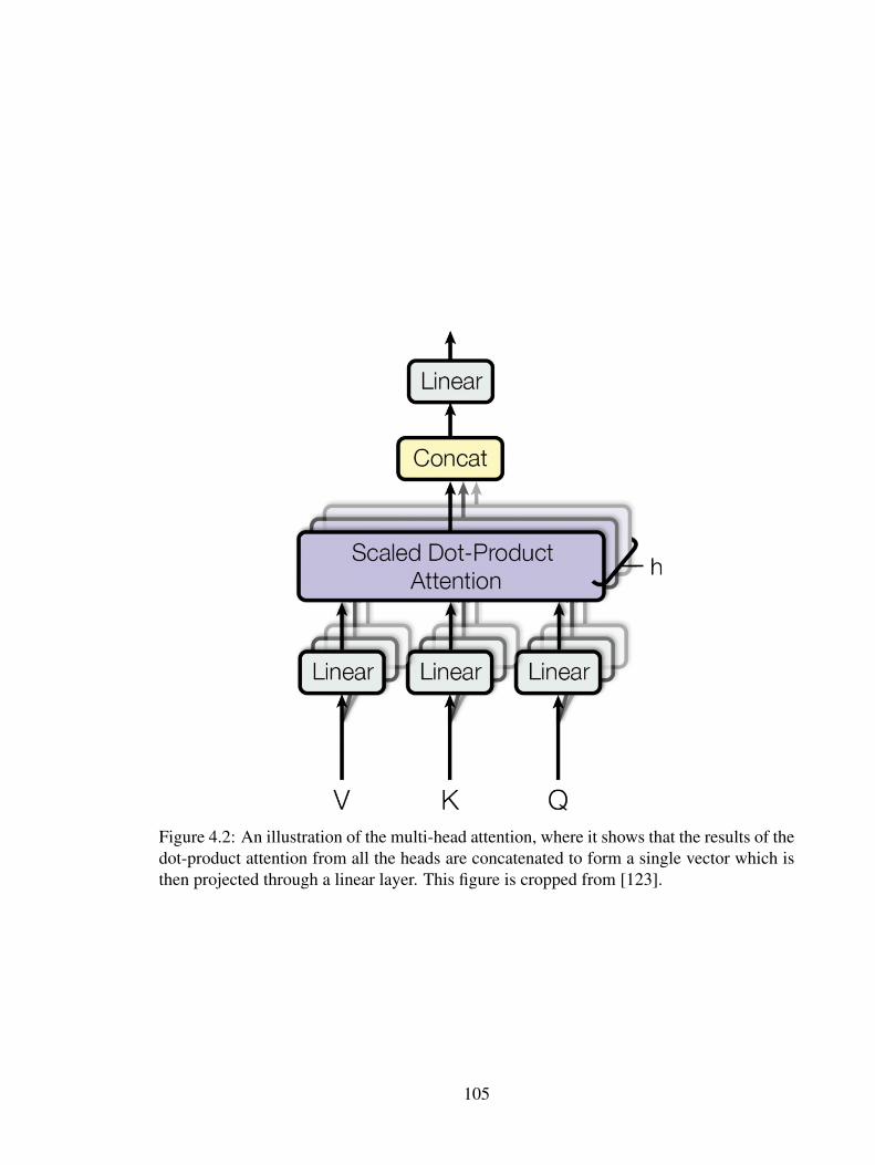
Figure 4.2: An illustration of the multi-head attention, where it shows that the results of thedot-product attention from all the heads are concatenated to form a single vector which isthen projected through a linear layer. This figure is cropped from [123].
105

length chunks (except the last one whose length can be shorter). As shown in Figure 4.3a,
the hidden state from the previous chunk is cached to extend keys and values from the
current chunk, providing extra history to be attended to. In this case, K (or V) is longer in
length than Q due to the prepended history. To alleviate the gradient explosion/vanishing
issue introduced in this kind of recurrent structure, gradient is set to not go beyond the
cached state, i.e.,
K𝑐 = [SG(K𝑐−1); K𝑐], V𝑐 = [SG(V𝑐−1); V𝑐] (4.3)
where 𝑐 is the chunk index, [·; ·] represents concatenation along the time dimension, and
SG(·) is the stop gradient operation.2 The memory usage and computation cost are both
reduced to 𝑂 (𝑇) when the chunk size is constant.
4.2.1 Look-ahead to the Future and Gradient Stop in His-
tory
Our initial experiments showed that only having history to the left is not sufficient for
a good performance in wake word detection. So we also allow a chunk to “look-ahead” to
the next chunk to get future context when making predictions from the current chunk. For
the right context, the gradient in back-propagation does not just stop at 𝐾𝑐+1 and 𝑉𝑐+1, but
rather goes all the way down to the input within the chunk 𝑐 + 1. On the other hand we
2 For example, this would be Tensor.detach() in PyTorch [88].
106

chunk c-1 chunk c
l
l-1
l+1
(a) Dependency on the previous layer of the previous chunk.
chunk c-1 chunk c
l
l-1
l+1
(b) Dependency on the same layer of the previous chunk.
Figure 4.3: Two different type of nodes dependency when computing self-attention instreaming Transformers. The figures use 3-layer networks with 2 chunks (delimited bythe thick vertical line in each sub-figure) of size 2 as examples. The grey arcs illustratethe nodes dependency within the current chunk, while the green arcs show the dependencyfrom the current chunk to the previous one.
107
can optionally treat the left context (i.e. the history state) the same way as well. Intuitively,
permitting more information (i.e. gradient flow back-propagated from the loss) while the
weights are being updated should always be beneficial, as long as their gradient flow is
constrained within a fixed range of time steps. This can be achieved by splicing the left
chunk together with the current chunk and then only selecting the output of the current
chunk for loss evaluation, at the cost of having one more forward computation for each
chunk by not caching them. We will show a performance comparison between with and
without such state-caching in the experiments.
4.2.2 Dependency on the Previous Chunk from the Same
Layer
Note that when there are multiple stacked self-attention layers, the output of the 𝑐-
th chunk of the 𝑙-th layer actually depends on the output of the (𝑐 − 1)-th chunk of the
(𝑙 − 1)-th layer. So the receptive field of each chunk grows linearly with the number of the
self-attention layers, and the current chunk does not have access to previous chunks in the
same layer (Figure 4.3a). This may limit the model’s temporal modeling capability as not
all parts of the network within the receptive field are utilized. Hence, we take the output
from the previous chunk in the same layer, and prepend it to the key and value. Formally,
108

let H = [h1, . . . , h𝑇 ] ∈ R𝑇×𝑑ℎ where h𝑖 is defined in Eq. (4.2). Then Eq. (4.3) becomes:
K𝑙
𝑐 = [SG(H𝑙𝑐−1); K𝑙
𝑐], V𝑙
𝑐 = [SG(H𝑙𝑐−1); V𝑙
𝑐] (4.4)
where we use superscript 𝑙 to emphasize tensors from the same layer. Figure 4.3b illustrates
nodes dependency in such computation flows.
4.2.3 Positional Embedding
The self-attention in Transformers is invariant to sequence reordering, i.e., any permu-
tations of the input sequence will yield exactly the same output for each frame. So it is
crucial to encode the positions. The original Transformer [123] employs deterministic si-
nusoidal functions to encode absolute positions. In our chunk-streaming setting, we can
also enable this by adding an offset to the frame positions within each chunk. However,
since our goal for wake word detection is just to spot the word rather than recognize the
whole utterance, a relative positional encoding may be suffice and even more appropriate,
as it does not matter what the absolute position the wake word is at. One type of relative
positional embedding, as shown in [111], encodes the relative positions from a query frame
to key/value frames in the self-attention blocks, and pairs of frames having the same posi-
tional offset share the same trainable embedding vector. The embedding vectors E ∈ R𝑑ℎ×𝑇
are then added to the key (optionally to the value as well) of each self-attention layer. So
109
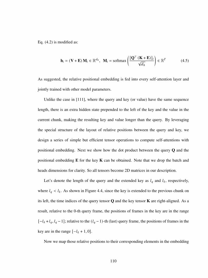
Eq. (4.2) is modified as:
h𝑖 = (V + E)M𝑖 ∈ R𝑑ℎ , M𝑖 = softmax([Q⊤ (K + E)]𝑖√
𝑑ℎ
)∈ R𝑇 (4.5)
As suggested, the relative positional embedding is fed into every self-attention layer and
jointly trained with other model parameters.
Unlike the case in [111], where the query and key (or value) have the same sequence
length, there is an extra hidden state prepended to the left of the key and the value in the
current chunk, making the resulting key and value longer than the query. By leveraging
the special structure of the layout of relative positions between the query and key, we
design a series of simple but efficient tensor operations to compute self-attentions with
positional embedding. Next we show how the dot product between the query Q and the
positional embedding E for the key K can be obtained. Note that we drop the batch and
heads dimensions for clarity. So all tensors become 2D matrices in our description.
Let’s denote the length of the query and the extended key as 𝑙𝑞 and 𝑙𝑘 , respectively,
where 𝑙𝑞 < 𝑙𝑘 . As shown in Figure 4.4, since the key is extended to the previous chunk on
its left, the time indices of the query tensor Q and the key tensor K are right-aligned. As a
result, relative to the 0-th query frame, the positions of frames in the key are in the range
[−𝑙𝑘 + 𝑙𝑞, 𝑙𝑞 − 1]; relative to the (𝑙𝑞 − 1)-th (last) query frame, the positions of frames in the
key are in the range [−𝑙𝑘 + 1, 0].
Now we map those relative positions to their corresponding elements in the embedding
110

Figure 4.4: The illustration of how relative positions are obtained in the streaming setting.the length of K 𝑙𝑘 is larger than the length of Q 𝑙𝑞 and they are right-aligned becausethe second half of K falls in the same chunk as Q. The dashed lines connecting to thesame point in Q denotes the range of all the positions in K w.r.t. that point. They are[−𝑙𝑘 + 𝑙𝑞, 𝑙𝑞 − 1] w.r.t. the 0-th (left-most) frame in Q, and [−𝑙𝑘 + 1, 0] w.r.t. the (𝑙𝑞 − 1)-th(right-most) frame in Q.
111

matrix. There are (2𝑙𝑘 − 1) possible relative positions from the query to the key in the
range [−𝑙𝑘 + 1, 𝑙𝑘 − 1], given that the key length 𝑙𝑘 is larger than the query length 𝑙𝑘 ,
leading to an embedding matrix E ∈ R𝑑ℎ×(2𝑙𝑘−1) . However, not all the integers that fall
within that range are being used in our case. Actually from Fig 4.4 and the description
from the previous paragraph, we can see that the “active” range is [−𝑙𝑘 + 1, 𝑙𝑞 − 1] =
[−𝑙𝑘 + 𝑙𝑞, 𝑙𝑞 − 1] ∪ [−𝑙𝑘 + 1, 0]. In other words, the last 𝑙𝑘 − 𝑙𝑞 positions in the embedding
matrix E are never used. Specifically, we first compute its dot product with the query Q,
resulting in a matrix M = Q⊤E ∈ R𝑙𝑞×(2𝑙𝑘−1) . Then for the 𝑖-th row in M, we select 𝑙𝑘
consecutive elements corresponding to 𝑙𝑘 different relative positions from the 𝑖-th frame
in the query to each frame in the key, and rearrange them into M′ ∈ R𝑙𝑞×𝑙𝑘 . This process
is illustrated in Figure 4.5. In the 0-th row, we keep those corresponding to the relative
positions in the range [−𝑙𝑘 + 𝑙𝑞, 𝑙𝑞−1]; in the 𝑖-th row, the range is left shifted by 1 from the
one in the (𝑖−1)-th row; finally in the (𝑙𝑞 −1)-th row, the range would be [−𝑙𝑘 +1, 0]. This
process can be conveniently implemented by reusing most of the memory configuration
from M for M′without copying the underlying storage of M, and then doing the following3:
1. Point M′ to the position of the first yellow cell in M, i.e., the (𝑙𝑞 − 1)-th position.
2. Modify the row stride of M′ from 𝑙𝑘 to (𝑙𝑘 − 1).
3. Modify the number of columns of M′ from (2𝑙𝑘 − 1) to 𝑙𝑘 .
The procedure when adding the embedding to the value V is very similar. Let A =
3In PyTorch, these can be conveniently implemented using Tensor.as_strided().
112

Figure 4.5: The process of selecting relevant cells from the matrix M ∈ R𝑙𝑞×(2𝑙𝑘−1) (left)and rearranging them into M′ ∈ R𝑙𝑞×𝑙𝑘 (right). The relevant cells are in yellow, and othersare unselected. Note that the position of yellow block in one row of M is left shifted by 1cell from the yellow block in the row above.
[a1, . . . , a𝑇 ] ∈ R𝑙𝑞×𝑙𝑘 where a𝑖 is defined in Eq. (4.5). Then the tensorized version of Eq.
(4.5) with the length of the query 𝑙𝑞 and the length of the extended value 𝑙𝑣 = 𝑙𝑘 is:
H = (V + E′) A⊤ ∈ R𝑑ℎ×𝑙𝑞 (4.6)
where E′ ∈ R𝑑ℎ×𝑙𝑘 is as follows:
1. Duplicate E ∈ R𝑑ℎ×(2𝑙𝑘−1) 𝑙𝑞 times along a new dimension by creating a new view on
the underlying storage without allocating new memory.4. Now we have an interme-
diate tensor E′′ ∈ R𝑑ℎ×𝑙𝑞×(2𝑙𝑘−1) .
2. Follow the steps for transforming M to M′, but this time apply them to E′′ to obtain
E′.4 For example, this would be Tensor.expand() in PyTorch.
113

Note that although E′′ is 3-dimensional, the operations applied along the 0-th dimension are
all identical. Again it is very efficient as there is no memory copy or allocation involved.
4.3 Experiments
4.3.1 The Dataset
We use the Mobvoi (SLR87) dataset5 [48] including two wake words: “Hi Xiaowen”
and “Nihao Wenwen”. It contains 144 hrs training data with 43,625 out of 174,592 positive
examples, and 74 hrs test data with 21,282 out of 73,459 positive examples. We do not
report results on the other datasets mentioned in Chapter 3, because both the numbers
reported there and in our own experiments are too good (FRR < 0.1%) to demonstrate any
significant improvements.
4.3.2 Experimental Settings
All the experiments in this paper are conducted in ESPRESSO, a PyTorch-based end-
to-end ASR toolkit [130], using PYCHAIN, a fully parallelized PyTorch implementation of
LF-MMI [110].
We follow exactly the same data preparation and preprocessing pipeline as those in
[132] (also in Chapter 3), including HMM and decoding graph topolopies, feature extrac-
5 https://www.openslr.org/87
114

tion, negative recording sub-segmentation, and data augmentations. During evaluation,
when one of the two wake words is considered, the other one is treated as a negative ex-
ample. The operating points are obtained by varying the positive path cost while fixing the
negative path cost at 0 in the decoding graph. It it worth mentioning that all the results
reported here are from an offline decoding procedure, as currently Kaldi [96] does not sup-
port online decoding with PyTorch-trained neural acoustic models. However, we believe
that the offline decoding results would not deviate significantly from the online ones.
The baseline system is a 5-layer dilated 1D convolutional network with 48 filters and the
kernel size of 5 for each layer, leading to 30 frames for both left and right context (25% less
than that in [132]) and only 58k parameters (60% less than that in [132]). For the streaming
Transformer models, the first two layers are 1D convolution. They are then followed by
3 self-attention layers, with an embedding dimension of 32, and 4 heads resulting in 48k
parameters without any relative embedding. See Table 4.1 for model sizes with different
relative embedding settings. To make sure that the outputs can “see” approximately the
same amount of context as those in the baseline, the chunk size is set to 27, so that in
the no state-caching setting the right-most frame in a chunk depends on 27 input frames
(still smaller than 30) as its right context; in the state-caching case, the receptive field
covers one more chunk (or 27 more frames) on the left, as it increases linearly when the
number of self-attention layers increases. Our experiments suggest 27 is the optimal in this
setting: a smaller chunk hurts the performance, and a larger one does not have significantly
improvement but incurs more latency.
115
All the models are optimized using Adam with an initial learning rate 10−3 , and then
halved if the validation loss at the end of an epoch does not improve over the previous
epoch. The training process stops if the number of epochs exceeds 15, or the learning
rate is less than 10−5. We found that learning rate warm-up is not necessary to train our
Transformer-based systems, probably due to the relatively simple supervisions in our task.
4.3.3 Streaming Transformers with State-caching
We first evaluate our streaming Transformer models with state-caching. The results
are reported in Table 4.1, as false rejection rate (FRR) at 0.5 false alarms per hour (FAH).
If we only rely on the current chunk and the cached state from the previous chunk but
without taking any look-ahead to the future chunk, the detection results (see row 2 in Table
4.1) are much worse than the baseline. It is actually expected, as the symmetric property
of convolution kernels allows the network to take future frames into consideration. This
validates that look-head to the future frames is important in the chunk-wise training of
Transformers.
Then adding absolute positional embedding seems not to improve the performance sig-
nificantly. One possible explanation could be: the goal of the wake word detection is not
to transcribe the whole recording, but just spot the word of interest, where the absolute
encoding of positions do not have too much effective impact.
On the contrary, when we add relative positional embedding to the key of self-attention
116

Table 4.1: Results of streaming Transformers with state-caching.
#ParamsFRR(%) at FAH=0.5
Hi Xiaowen Nihao Wenwen
1D Conv. (baseline)6 58k 0.8 0.8Transformer (w/o look-ahead) 48k 3.5 4.7
+look-ahead to next chunk 48k 1.3 1.2+abs. emb. 48k 1.2 1.2+rel. emb. to key 52k 1.0 1.1
+rel. emb. to value 57k 0.7 0.5
layers instead, there is a slight improvement over adding the absolute embedding, which
supports our hypothesis that the relative embedding makes more sense in such task.
When the embedding is also added to the value, FRR reaches 0.7% and 0.5% at
FAH=0.5 for the two wake words respectively (i.e., 25% relative improvement over the
baseline on average), showing that the embedding is not only useful when calculating the
attention weights, but also beneficial when encoding the positions into the layer’s hidden
values.
4.3.4 Streaming Transformers without State-caching
Next we explore whether back-propagating the gradient into the history state helps
train a better model. As we mentioned in Sec. 4.2.1, this can be done by concatenating
the current chunk with the previous chunk of input, instead of caching the internal state
6 We do not compare with other systems, because to our best knowledge this baseline system is the state-of-the-art reported on the same dataset at the time of writing this dissertation.
117

Table 4.2: Results of streaming Transformers without state-caching.
#ParamsFRR(%) at FAH=0.5
Hi Xiaowen Nihao Wenwen
1D Conv. (baseline) 58k 0.8 0.8Transformer (w/ look-ahead) 48k 1.0 1.1
+abs. emb. 48k 0.8 0.8+rel. emb. to key 52k 0.6 0.7
+rel. emb. to value 57k 0.6 0.6
of the previous chunk. Table 4.2 shows several results. By looking at Table 4.2 itself, we
observe a similar trend as that in the state-caching model from Table 4.1: relative positional
embedding is advantageous over the absolute sinusoidal positional embedding, and adding
the embedding to both key and value is again the best. Furthermore, by comparing the
rows in Table 4.2 with their corresponding entries in Table 4.1, we observe that, except
for the case in the last row, regardless of the choice of positional embedding and how
it is applied, the models without state-caching outperform models with state-caching. It
demonstrates the benefit of updating the model parameters with more gradient information
back-propagated from the current chunk into the previous chunk. However in the case
where relative positional embedding is also added to the value, the gap seems diminished,
suggesting that by utilizing the positional embedding in a better way, there is no need to
recompute the part of the cached state in order to reach the best performance.
We provide DET curves of the baseline convolutional network and the two proposed
118

streaming Transformers in Figure 4.6, for a more comprehensive demonstration of their
performance difference, over an entire operating range.
0.00 0.25 0.50 0.75 1.00 1.25 1.50 1.75 2.00False Alarms per hour
0.0
0.2
0.4
0.6
0.8
1.0
1.2
1.4
1.6
False
Rej
ectio
n Ra
te (%
)
1D Conv. 'Hi Xiaowen'1D Conv. 'Nihao Wenwen'states-caching Trans. 'Hi Xiaowen'states-caching Trans. 'Nihao Wenwen'non-states-caching Trans. 'Hi Xiaowen'non-states-caching Trans. 'Nihao Wenwen'
DET curve
Figure 4.6: DET curves for the baseline 1D convolutional network and our two proposedstreaming Transformers.
4.3.5 Streaming Transformers with Same-layer Depen-
dency
We next explore the architectural variant introduced in Sec. 4.2.2. Note from Eq. (4.2)
that the column vectors in H𝑙𝑐−1 are all in range(V𝑙
𝑐−1), i.e., the column vectors of H𝑙𝑐−1 lie
119

in the space spanned by the the columns of V𝑙𝑐−1. Therefore, concatenation of H𝑙
𝑐−1 and
V𝑙𝑐 together along the column dimension as shown in Eq. (4.4) is legitimate. However,
if the relative positional embedding is added to the value tensor H𝑙𝑐−1 as shown in Eq.
(4.5), the columns in H𝑙𝑐−1 would no longer be in the same space as range(V𝑙
𝑐). Then it is
problematic to concatenate H𝑙𝑐−1 and V𝑙
𝑐 together. In addition, because H𝑙𝑐−1 is going to be
concatenated to both K𝑙𝑐 and V𝑙
𝑐, we need to make sure that the columns of K𝑙𝑐 and V𝑙
𝑐 are
in the same space.
Our solution to these issues—which arises due to the same-layer dependency—is to
only add the positional embedding to K𝑙𝑐. So Eq. (4.5) is modified as:
h𝑖 = VM𝑖 ∈ R𝑑ℎ , M𝑖 = softmax([Q⊤ (K + E)]𝑖
)∈ R𝑇 (4.7)
Also, the projection weight matrices for the key/value in Eq. (4.1), i.e. W𝐾 and W𝑉
respectively, are tied together, so that K𝑙𝑐 == V𝑙
𝑐 always holds. However, the model with
such a configuration only achieves FRR=1.3% at FAH=0.5. When absolute embedding is
used, FRR=1.1% at the same FAH. This contradicts the observations in [73], [137] where
same-layer dependency was found to be more advantageous for ASR and it was attributed
to the fact that the receptive field is maximized at every layer7.
7 They did not mention the type of positional embedding being used.
120

4.3.6 Resources Consumption
According to Eq. 3.7 in Section 3.3.11, the convolution baseline involves 43, 000 × 𝑇
floating point operations.
For the chunk-wise streaming transformers with state-caching, as the “current chunk”
will be served as the cached history for the next chunk, we amortize the computation of
history across the entire input audio frames and ignore the boundary case for the first chunk,
i.e., for every chunk of the input we always assume its history is available and do not take it
into consideration we calculating the computation cost. On the contrary, the future chunks
are not cached and thus account for the computation cost. Therefore when the chunk size
is 27, the length of the query is 54 (“current chunk” + “future chunk”) and the length of
the key/value is 81 (“history chunk” + “current chunk” + “future chunk”). It turns out that
there are about 132, 000 × 𝑇 floating point operations for such an architecture.
A larger number of floating point operations does not necessarily means faster infer-
ence. Actually speed is determined by several factors, including parallelization of compu-
tation and CUDA kernel optimization. To directly measure the speed, we run the forward
pass of the neural networks on all the examples from the same test set (74 hours) with
a single NVIDIA GeForce GTX 1080 Ti GPU. It takes 445 seconds for the baseline 1D
convolutional network, and 286 seconds for the chunk-wise streaming transformers with
state-caching. Note that it is not straightforward to draw a conclusion such as one network
is advantageous to the other one, as PyTorch may apply different optimization strategies
121
to different network configurations; but at least it can been shown that the transformer
network does not have obvious disadvantages in terms of inference speed.
Next we show the peak memory usage of the two networks using the same method as
explained in Section 3.3.11: the peak memory usage is 120 MB for the 1D convolution and
399 MB for the chunk-wise streaming transformers with state-caching. So apparently the
transformer model consumes 3 times more memory than the convolutional one. Note that
the neural networks in this chapter are just prototype systems implemented in PyTorch, and
they are not intended for deployment. Hence the absolute memory usage is not very in-
dicative for real applications. However, our main purpose here is to show the difference in
memory consumption between the convolution baseline and the proposed streaming Trans-
former.
4.4 Chapter Summary
Transformers are power neural networks that have shown their modeling strength in
a variety of NLP and ASR tasks. In this chapter we investigated their performance in
wake word detection. Due to the discrepancy between the streaming nature of wake word
detection and the whole sequence dependency of self-attention in the basic transformer,
we explored various aspects of chunk-wise streaming transformers, including how look-
ahead of the future chunk, and different gradient stopping, layer dependency, and positional
embedding strategies could affect the system performance. Our experiments show that
122

streaming transformers achieve better detection performance compared to 1D convolutions
with similar model and receptive field sizes on the public Mobvoi (SLR87) dataset using
the state-of-the-art alignment-free LF-MMI system. Specifically, we found that:
• Look-ahead to the future chunk is necessary for the streaming Transformer model to
collect enough context information and make reliable chunk-wise predictions.
• Relative positional embedding is more suitable than absolute positional embedding
(with chunk offsets) and provided additional gain for wake word detection with
streaming Transformers, because relative positions are more informative for the
detection task. Moreover, adding the embedding to both keys and values of self-
attention layers is better than only adding to keys.
• Training Transformer without state-caching yields better detection performance than
with state-caching in most cases, as the former one allows more weights to be up-
dated according to the gradient information back-propagated across all layers. But
no caching requires extra computational cost of overlapping chunks.
• Fortunately, when relative positional embedding is added to both keys and values,
the performance of the Transformer with state-caching is on par with the one without
state-caching.
• Normally the chunk of one layer depends on the previous chunk from the previous
layer when calculating self-attention in chunk-wise streaming Transformers. We also
123

tried a variation where the chunk depends on the previous chunk from the same layer.
However, it did not lead to better performance.
Along the way we also proposed a series of simple tensor operations to efficiently com-
pute the self-attention in the streaming setting when relative positional embedding is in-
volved.
Unlike basic Transformers, chunk-wise streaming Transformers have linear time and
space complexity with respect to the frame length 𝑇 . Specifically, if the chunk-width is𝑊 ,
the time complexity is 𝑂 (𝑊 ·𝑇) = 𝑂 (𝑊2 ·𝑇/𝑊). If the constant factor𝑊 is larger than the
kernel size of a convolutional layer, which is normally the case, the number of float point
operations in streaming Transformers is still more than that in convolutions (as shown in
Section 4.3.6). Some recent work [20], [57] of improving efficiency of self-attention has
the potential to further reduce the complexity.
124

Chapter 5
End-to-end Anchored Speech
Recognition
In the previous two chapters, we proposed methods to detect wake words in audio
stream [132], [133]. In this chapter we will show how we can leverage the detected wake
word to improve the ASR performance for voice-controlled house-hold devices. We would
like to teach the device to ignore speech that is not intended for it. Specifically, our tech-
nique takes an acoustic snapshot of the wake word and compares subsequent speech to it.
Speech whose acoustics match those of the wake word is judged to be intended for the de-
vice, and all other speech is treated as background noise and ignored. Rather than training a
separate neural network to make this discrimination, we integrate our wake-word-matching
mechanism into a standard ASR system. We will show how we design our attention-based
encoder-decoder ASR model to realize this task, and how much improvement is obtained
125

on the live data collected by Amazon Alexa Echo, a popular house-hold device, as well as
on a simulated data set. Specifically, our contributions in this chapter are: we propose two
end-to-end models to tackle this problem with information extracted from the anchored
segment. The anchored segment refers to the wake word part of an audio stream, which
contains valuable speaker information that can be used to suppress interfering speech and
background noise. The first method is called Multi-source Attention where the attention
mechanism takes both the speaker information and decoder state into consideration. The
second method directly learns a frame-level mask on top of the encoder output. We also
explore a multi-task learning setup where we use the ground truth of the mask to guide
the learner. Given that audio data with interfering speech is rare in our training data set,
we also propose a way to synthesize “noisy” speech from “clean” speech to mitigate the
mismatch between training and test data. The work in this chapter was published in [131]
and [130].
5.1 Introduction
We tackle the ASR problem in the scenario where a foreground speaker first wakes
up a voice-controlled device with an “wake word”, and the speech after the wake word is
possibly interfered with by background speech from other people or media. Consider the
following example:
SPEAKER 1: Alexa, play rock music.
126

Figure 5.1: An illustration of anchored speech recognition. We would like to suppressspeech from Speaker 2 and only recognize that from Speaker 1, because it is Speaker 1who says “Alexa” to the device.
SPEAKER 2: Stop.
Here the wake word is “Alexa”, and thus the utterance by speaker 1 is considered as
device-directed speech, while the utterance by speaker 2 is the interfering speech. Our
goal is to extract information from the wake word in order to recognize the device-directed
speech and ignore the interfering speech. We name this task anchored speech recogni-
tion (Figure 5.1). The challenge of this task is to learn a speaker representation from a
short segment corresponding to the wake word. Several techniques have been proposed
for learning speaker representations, e.g., i-vector [27], [106], mean-variance normaliza-
tion [72], maximum likelihood linear regression (MLLR) [67]. With the recent progress in
deep learning, neural networks are used to learn speaker embeddings for speaker verifica-
tion/recognition [42], [77], [115], [122]. More relevant to our task, two methods—anchor
mean subtraction (AMS) and an encoder-decoder network—are proposed to detect desired
speech by extracting speaker characteristics from the wake word [75]. This work is further
extended for acoustic modeling in hybrid ASR systems [55]. However, they simply con-
catenate the vector characterizing speakers to the input acoustic feature vector, and there
is no explicit mechanism of ignoring undesired speech. In fact, the speaker feature only
127

plays the role of a biasing term to the input feature. Therefore, it does not have enough ca-
pacity of distinguishing speaker difference between device-directed and interfering speech.
target-speaker mask estimation is also explored for target speaker extraction [28], [128].
Specifically, [28] uses an adaption utterance (corresponding to wake word segment in our
problem) to estimate a weight vector that is then leveraged to eventually estimate the target
speaker mask. But this method is not applicable to our problem, since it assumes the tar-
get speech is present during the entire utterance, while in our problem the device-directed
speech can be present in several parts of the whole utterance. [128] proposes what they
called “deep extractor network” for speaker-aware source separation. Our method shares
some spirit with [128] in that we both compute the similarity between two embedding
vectors to estimate masks, and ours directly addresses the ASR problem.
Recently, much work has been done towards end-to-end approaches for speech recog-
nition [7], [13], [18], [22], [35], [37]. These approaches typically have a single neu-
ral network model to replace previous independently-trained components, namely, acous-
tic, language, and pronunciation models from hybrid HMM systems. End-to-end models
greatly alleviate the complexity of building an ASR system. Among end-to-end models, the
attention-based encoder-decoder models [2], [7] do not assume conditional independence
for output labels as CTC based models [36], [37] do.
We propose two end-to-end models for anchored speech recognition, focusing on the
case where each frame is either completely from device-directed speech or completely
from interfering speech, but not a mixture of both [11], [28]. They are both based on the
128

attention-based encoder-decoder models. The attention mechanism provides an explicit
way of aligning each output symbol with different input frames, enabling selective decod-
ing from an audio, i.e., only decode desired speech that is being uttered in some parts of
the entire audio stream. In the first method, we incorporate the speaker information when
calculating the attention energy, which leads to an anchor-aware soft alignment between
the decoder state and encoder output. The second method learns a frame-level mask on
top of the encoder, where the mask can optionally be learned in the multi-task framework
if the ground-truth mask is given. This method will pre-select the encoder output before
the attention energy is calculated. Furthermore, since the training data is often relatively
clean, in the sense that it contains device-directed speech only, we propose a method to
synthesize “noisy” speech from “clean” speech, mitigating the mismatch between training
and test data.
We conduct experiments on a training corpus consisting of 1200 hours of live data in
English from Amazon Echo. The results demonstrate a significant WER relative gain of
12-15% in test sets with interfering background speech. However, a method that suppresses
non-anchored speech may also accidentally suppress the target speaker, especially when no
interfering speech is present but the system expects there to be some. Indeed, for a test set
that contains only device-directed speech, we see a small relative WER degradation from
the proposed method, ranging from 1.5% to 3%. We also demonstrate the results of the
proposed models on the data simulated from the public data set Wall Street Journal (WSJ)
[89].
129
5.2 Model Overview
5.2.1 Attention-based Encoder-Decoder Model
The basic attention-based encoder-decoder model typically consists of 3 modules as
depicted in Fig 5.2:
1. An encoder transforming a sequence of input features x1:𝐿 into a high-level repre-
sentation of the features h1:𝑇 through a stack of convolution/recurrent layers, where
𝑇 ≤ 𝐿 due to possible frame down-sampling.
2. An attention module summarizing the output of the encoder h1:𝑇 into a fixed length
context vector c𝑛 at each output step for 𝑛 ∈ [1, . . . , 𝑁], which determines parts of the
sequence h1:𝑇 to be attended to in order to predict the output symbol 𝑦𝑛. Typically, the
context vector is more compact than the original input. The attention mechanism’s
decision is typically based on the current states of both the encoder and decoder
3. A decoder module taking the context vector c𝑛 as input and predicting the next sym-
bol 𝑦𝑛 given the history of previous symbols 𝑦1:𝑛−1.
130

h1 h2 h3 hT
Attention
cn−1 qn−1
yn−1
Decoder
qn
yn
Encoder
x1:L
yn−2 yn−1
Figure 5.2: Attention-based Encoder-Decoder Model. It is an illustration in the case ofa one-layer decoder. If there are more layers, as in our experiments, an updated contextvector c𝑛 will also be fed into each of the upper layers in the decoder at the time step 𝑛.
The entire model can be formulated as follows:
h1:𝑇 = Encoder(x1:𝐿) (5.1)
𝛼𝑛,𝑡 = Attention(q𝑛, h𝑡) (5.2)
c𝑛 =∑𝑡
𝛼𝑛,𝑡h𝑡 (5.3)
q𝑛 = Decoder(q𝑛−1, [𝑦𝑛−1; c𝑛−1]) (5.4)
𝑦𝑛 = arg max𝑣(W 𝑓 q𝑛 + b 𝑓 ) (5.5)
Although our proposed methods do not limit themselves to any particular attention mecha-
nism, we choose the Bahdanau Attention [2] as the attention function for our experiments.
131

So Eq. (5.2) takes the form of:
𝜔𝑛,𝑡 = v⊤ tanh(W𝑞q𝑛 +Wℎh𝑡 + b) (5.6)
𝛼𝑛,𝑡 = softmax(𝜔𝑛,𝑡) (5.7)
5.2.2 Multi-source Attention Model
Our first approach is based on the intuition that the attention mechanism should consider
both the speaker information and the decoder state. It simply adds an input to the attention
mechanism. In addition to receiving information about the current states of the encoder
and decoder networks, our modified attention mechanism also receives the raw frame data
corresponding to the wake word. During training, the attention mechanism automatically
learns which acoustic characteristics, that are similar to the wake word, to look for in
subsequent speech.
When computing the attention weights, in addition to conditioning on the decoder state,
the speaker information extracted from the frames of the wake word is also utilized. In our
scenario, the device-directed speech and the wake word are uttered by the same speaker,
while the interfering background speech is from a different speaker. Therefore, the attention
mechanism can be augmented by placing more attention probability mass on frames that
are similar to the anchor word in terms of speaker characteristics.
Formally speaking, the wake word segment is further denoted as w1:𝐿 ′. We add another
132

encoder (S-Encoder) to be applied on both w1:𝐿 ′ and x1:𝐿 to generate a fixed-length vector
w and a variable length sequence u1:𝑇 respectively:
w = Pooling(S-Encoder(w1:𝐿 ′)) (5.8)
u1:𝑇 = S-Encoder(x1:𝐿) (5.9)
As shown above, S-Encoder extracts speaker characteristics from the acoustic features. In
our experiments, the pooling function is implemented as Max-pooling across all output
frames if S-Encoder is a convolutional network, or picking the hidden state of the last
frame if S-Encoder is a recurrent network. Rather than being appended to acoustic feature
vector and fed into the decoder as proposed in [55] (which we tried in our preliminary
experiments but did not perform well), w is directly involved in computing the attention
weights. Specifically, Eq. (5.7) and Eq. (5.3) are replaced by:
𝜙𝑡 = Similarity(u𝑡 , w) (5.10)
𝛼anchor_aware𝑛,𝑡 = softmax(𝜔𝑛,𝑡 + 𝑔 · 𝜙𝑡) (5.11)
c𝑛 =∑𝑡
𝛼anchor_aware𝑛,𝑡 h𝑡 (5.12)
where 𝑔 is a trainable scalar used to automatically adjust the relative contribution from
the speaker acoustic information. Similarity(·, ·) is implemented as dot-product in our
experiments. As a result, the attention weights are essentially computed from two different
133

sources: the ASR decoding state, and the confidence of a decision on whether each frame
comprises the device-directed speech. We call this model Multi-source Attention to reflect
the way the attention weights are computed.
5.2.3 Mask-based Model
The Multi-source Attention model jointly considers speaker characteristic and ASR
decoder state when calculating the attention weights. However, since the attention weights
are normalized with a softmax function, whether each frame needs to be ignored is not
independently decided, which reduces the modeling flexibility in frame selection.
As the second approach we train the network more explicitly to emphasize input speech
whose acoustic profile matches that of the wake word, which is named the Mask-based
model. We add a mechanism that directly compares the wake word acoustics with those of
subsequent speech. Then we use the result of that comparison as an input to a mechanism
that learns to suppress (or “mask out”) some elements of the encoder’s output before they
pass to the attention module.
Specifically, a frame-wise mask on top of the encoder1 is estimated by leveraging the
speaker acoustic information contained in the anchor word and the actual recognition ut-
terance. The attention mechanism is then performed on the masked feature representation.
Compared with the Multi-source Attention model, attention in the Mask-based model only
focuses on remaining frames after masking, and for each frame it is independently de-1Here “frame-wise” actually means frame-wise after down-sampling, in accordance with the frame down-
sampling in the encoder network (see Section 5.4.1 for details).
134

cided whether to be masked out based on their acoustic similarity. Formally, Eq. (5.6) and
Eq. (5.3) are modified as:
𝜙𝑡 = sigmoid(𝑔 · Similarity(u𝑡 , w)) (5.13)
hmasked𝑡 = 𝜙𝑡h𝑡 (5.14)
𝜔𝑛,𝑡 = v⊤ tanh(W𝑞q𝑛 +Wℎhmasked𝑡 + b) (5.15)
c𝑛 =∑𝑡
𝛼𝑛,𝑡hmasked𝑡 (5.16)
where Similarity(·, ·) in Eq. (5.13) is dot-product as well.
5.3 Synthetic Data and Multi-task Training
5.3.1 Synthetic Data
Due to the difficulty of collecting a large amount of noisy speech from house-hold
devices and annotate them accurately, a problem we encountered in our task is: there is
very little training data that has the same condition as the test case. Some utterances in
the test set contain speech from two or more speakers (denoted as the “speaker change”
case), and some of the other utterances only contain background speech (denoted as the
“no desired speaker” case). In contrast, most of the training data does not have interfering
or background speech, making the model unable to learn to ignore.
135

In order to simulate the condition of the test case, we generate two types of synthetic
data for training:
• Synthetic Method 1: for an utterance, a random segment2 from another utterance
in the dataset is inserted at a random position after the wake word within this utter-
ance, while its transcript is unchanged (i.e. the transcript of the inserted utterance is
ignored).
• Synthetic Method 2: the entire utterance, excluding the wake word, is replaced by
another utterance, and its transcript is considered as empty.
Figure 5.3 illustrates the synthesising process. These two types of synthetic data simulate
the “speaker change” case and the “no desired speaker” case respectively. The synthetic and
device-directed data are mixed together to form our training data. The mixing proportion
is determined from experiments.
5.3.2 Multi-task Training for Mask-based Model
For the generated synthetic data, we know which frames come from the anchor speaker
and which not, i.e., we have the ground-truth or ideal mask for each synthetic utterance,
where the frames from the original utterance are labeled with “1”, and the other frames are
labeled with “0”. Using this ideal mask as an auxiliary target, we train the Mask-based
model in a multi-task way, where the overall loss is defined as a linear interpolation of the
2The frame length of a segment is uniformly sampled within the range [50,150] in our experiments. It ispossible that the randomly selected segment is purely non-speech or even silence.
136

<w> what’s the weather <w> play a song from frozen
<w> what’s the weather
<w> what’s the weather <w> play a song from frozen
<w> <SPACE>
Figure 5.3: Two types of synthetic data: Synthetic Method 1 (top) and 2 (bottom). Thesymbol ⟨W⟩ represents the wake-up word, and ⟨SPACE⟩ represents empty transcripts.
normal ASR cross-entropy loss and the binary-cross-entropy mask loss: (1 − _)LASR +
_Lmask.
The ground-truth mask provides a supervision signal to explicitly guide S-Encoder to
extract acoustic features that can better distinguish the inserted frames from those in the
original utterance. As will be shown in our experiments, the predicted mask is more accu-
rate in selecting desired frames for the decoder with the multi-task training.
137

5.4 Experiments
We provide experimental results on both simulated and real data to validate the power of
our proposed models in for anchored speech recognition. The simulated data is generated
based on our assumptions of real data, and thus is intended to verify that our proposed
models will behave as what it is supposed to be. Also, since we use the well-known public
dataset Wall Street Journal [89] (WSJ) for the simulation, people will get better sense
of how the proposed models performs compared to the baseline. One the other hand, the
experiments on the real data (which comes from real users of Amazon Alexa devices) show
the improvement in the real scenario. But absolute WER on the real data cannot be shared
due to privacy and proprietary considerations, and only relative changes in WER can be
reported here.
5.4.1 Experimental Settings
The WSJ corpus is for simulation. WSJ is an 80-hour English newspaper speech corpus
[89]. We use its dev93 set for model validation and eval92 set for evaluation. We simulate
the training/test data as follows: for each utterance, we randomly select a 2-second segment
from that utterance as a wake word. Then we apply the procedure described in Section 5.3.1
to eval92 to construct the simulated test set (referred to as “simulated”, while the original
eval92 set is referred to as “original”) to mimic the “speaker change” and “no desired
speaker” cases. Specifically, 60% of the utterances in the training set are kept unchanged,
138

16% are processed with Synthetic Method 1, and 24% are processed with Synthetic Method
2. The duration of the inserted segments are uniformly distributed in the range [3.0, 5.0]
seconds, with the additional constraint that the duration of an inserted segment should
not exceed 20% of the duration of the original example. All the experiments on WSJ
are done with the open-source toolkit ESPRESSO [130], where there exists a very strong
attention-based encoder-decoder baseline recipe on WSJ that we can leverage3. We extract
80-dimensional filterbank features + 3-dimensional pitch features for each frame with the
frame rate 10 milliseconds and window size of 25ms. The output targets are graphemes
with vocabulary size of 52. We only use paired data (i.e. transcribed speech data) for
training and do not apply any language model fusion technique as it is orthogonal to the
problem we are solving here.
For the real data experiment, we conduct our experiments on training data of 1200-
hour live segments in English collected from the Amazon Echo. Each utterance is hand-
transcribed and begins with the same wake word whose alignment with time is provided by
end-point detection [70], [76], [109], [112]. As we have mentioned, while the training data
is relatively clean and usually only contains device-directed speech, the test data is more
challenging and under mismatched conditions with training data: it may be noisy, may
contain background speech4, or may even contain no device-directed speech at all. In order
to evaluate the performance on both the matched and mismatched cases, two test sets are
3Available at https://github.com/freewym/espresso/blob/master/examples/asr_wsj/run.sh.
4background speech includes: 1) interfering speech from an actual non-device-directed speaker; and 2)multi-media speech, meaning that a television, radio, or other media device is playing back speech in thebackground.
139

formed: a “normal set” (25k words in transcripts) where utterances have a similar condition
as those in the training set, and a “hard set” (5.4k words in transcripts) containing the chal-
lenging utterances with interfering background speech. Note that both of the two test sets
are real data without any synthesis. We also prepare a development set (“normal”+“hard”)
with a similar size as the test sets for hyper-parameter tuning. For all the experiments, 64-
dimensional log filterbank energy features are extracted every 10ms with a window size of
25ms. The end-to-end systems are grapheme-based and the vocabulary size is 36, which is
determined by thresholding on the minimum number of character counts from the training
transcripts. Our implementation is based on the open-source toolkit OPENSEQ2SEQ [64].
Our baseline end-to-end model does not consider anchor words. Its encoder consists
of four convolutional layers with 4x frame and frequency down-sampling for WSJ, or
three convolutional layers resulting in 2x frame down-sampling and 8x frequency down-
sampling for the Amazon live data, followed by 3 Bi-directional LSTM [46] layers with
320 hidden units. The decoder consists of 3 unidirectional-LSTM layers with 320 hidden
units. The attention function is Bahdanau Attention [2]. The cross-entropy loss on charac-
ters is optimized using Adam [56], with an initial learning rate 0.001 which is then halved
if the metric on the validation set at the end of an epoch does not improve over the previ-
ous epoch for WSJ [130] (or the initial learning rate is 0.0008 which is then adjusted by
exponential decay for the Amazon live data). A beam search with beam size 60 for WSJ
(or 15 for the Amazon data) is adopted for decoding. The above setting is also used in our
proposed models.
140

5.4.2 Multi-source Attention Model vs. Baseline
S-Encoder consists of three convolution layers with the same architecture as that in the
baseline’s encoder.
First of all, we compare Multi-source Attention Model and the baseline trained on
device-directed-only Amazon live data or the original WSJ training data, i.e., without any
synthetic data. The results are shown in Table 5.1 and Table 5.2 respectively.
Table 5.1: Multi-source Attention Model vs. Baseline with device-directed-only trainingdata. The WER, substitution, insertion and deletion values are all normalized by the base-line WER on the “normal” set5. The normalization applies to all the tables throughout thischapter in the same way.
Model Training Set Test Set WER sub ins del WERR(%)
BaselineDevice-
directed-only
normal 1.000 0.715 0.108 0.177 —
hard 3.354 1.762 1.123 0.469 —
Mul-src.
Attn.
Device-
directed-only
normal 1.015 0.731 0.115 0.169 -1.5
hard 3.262 1.746 1.062 0.454 +2.8
Amazon live data The relative WER reduction (WERR) of Multi-source Attention on the
“hard” set is 2.8% and it is mostly due to a reduction in insertion errors. We also observe a
slight WER degradation of 1.5% relative on the “normal” set. It implies that the proposed
model is more robust to interfering background speech.5For example, if WER for the baseline is 5.0% for the “normal” set, and 25.0% for the “hard” set, then
the normalized values would be 1.000 and 5.000 respectively. Due to Amazon’s policy, we are unable topublicize the absolute WERs on Amazon Alexa’s customer data.
141
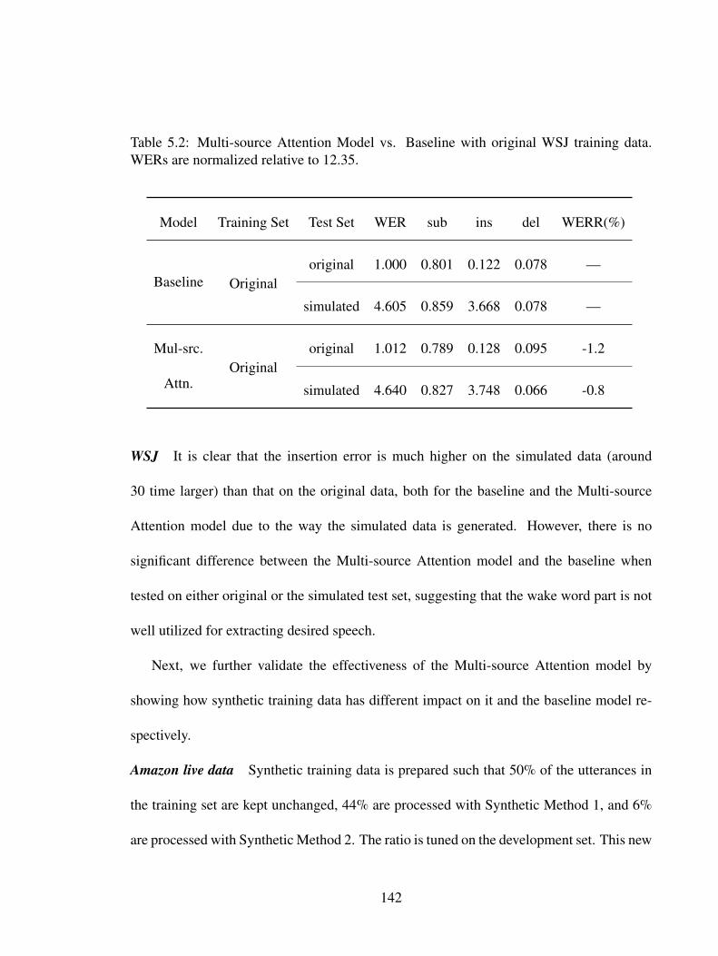
Table 5.2: Multi-source Attention Model vs. Baseline with original WSJ training data.WERs are normalized relative to 12.35.
Model Training Set Test Set WER sub ins del WERR(%)
Baseline Originaloriginal 1.000 0.801 0.122 0.078 —
simulated 4.605 0.859 3.668 0.078 —
Mul-src.
Attn.Original
original 1.012 0.789 0.128 0.095 -1.2
simulated 4.640 0.827 3.748 0.066 -0.8
WSJ It is clear that the insertion error is much higher on the simulated data (around
30 time larger) than that on the original data, both for the baseline and the Multi-source
Attention model due to the way the simulated data is generated. However, there is no
significant difference between the Multi-source Attention model and the baseline when
tested on either original or the simulated test set, suggesting that the wake word part is not
well utilized for extracting desired speech.
Next, we further validate the effectiveness of the Multi-source Attention model by
showing how synthetic training data has different impact on it and the baseline model re-
spectively.
Amazon live data Synthetic training data is prepared such that 50% of the utterances in
the training set are kept unchanged, 44% are processed with Synthetic Method 1, and 6%
are processed with Synthetic Method 2. The ratio is tuned on the development set. This new
142

training data is referred as “augmented” in all result tables. Table 5.3 exhibits the results.
For the baseline model, the performance degrades drastically when trained on augmented
data: the deletion errors on both of the “normal” and “hard” test sets get much higher. This
is expected since without the anchor word the model has no extra acoustic information of
which part of the utterance is desired, so that it tends to ignore frames randomly regardless
of whether they are actually from device-directed speech. On the contrary, for the Multi-
source Attention model the WERR (augmented vs. device-directly-only) on the “hard” set
is 12.5%, and WER on the “normal” set does not get worse. Moreover, the insertion errors
on the “hard” set get reduced while the deletion errors increase much less than that in the
case of the baseline model, indicating that by incorporating the anchor word information
the proposed model effectively improves the ability of focusing on device-directed speech
and ignoring others. This series of experiments also reveals significant benefits from using
the synthetic data with the proposed model. In total, the combination of the Multi-source
Attention model and augmented training data achieves 14.9% WERR on the “hard” set,
with only 1.5% degradation on the “normal” set.
143
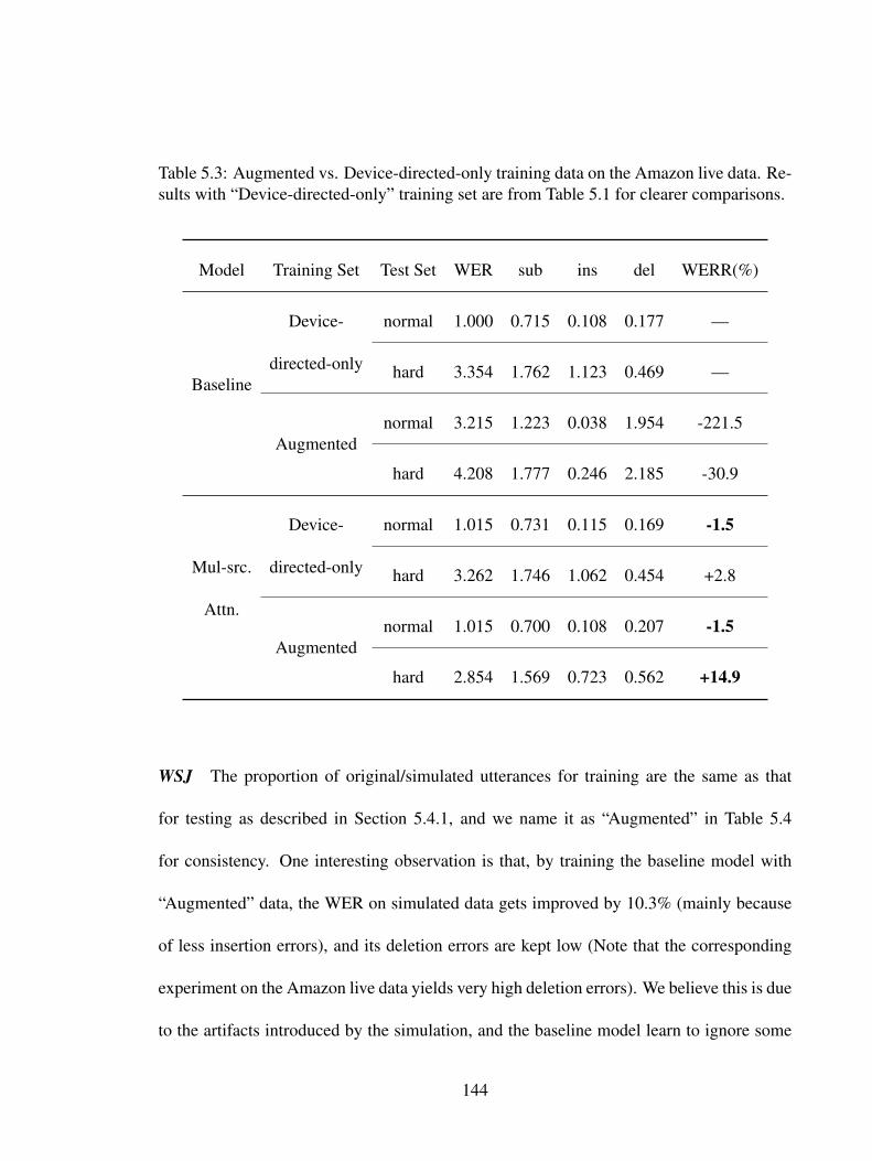
Table 5.3: Augmented vs. Device-directed-only training data on the Amazon live data. Re-sults with “Device-directed-only” training set are from Table 5.1 for clearer comparisons.
Model Training Set Test Set WER sub ins del WERR(%)
Baseline
Device-
directed-only
normal 1.000 0.715 0.108 0.177 —
hard 3.354 1.762 1.123 0.469 —
Augmentednormal 3.215 1.223 0.038 1.954 -221.5
hard 4.208 1.777 0.246 2.185 -30.9
Mul-src.
Attn.
Device-
directed-only
normal 1.015 0.731 0.115 0.169 -1.5
hard 3.262 1.746 1.062 0.454 +2.8
Augmentednormal 1.015 0.700 0.108 0.207 -1.5
hard 2.854 1.569 0.723 0.562 +14.9
WSJ The proportion of original/simulated utterances for training are the same as that
for testing as described in Section 5.4.1, and we name it as “Augmented” in Table 5.4
for consistency. One interesting observation is that, by training the baseline model with
“Augmented” data, the WER on simulated data gets improved by 10.3% (mainly because
of less insertion errors), and its deletion errors are kept low (Note that the corresponding
experiment on the Amazon live data yields very high deletion errors). We believe this is due
to the artifacts introduced by the simulation, and the baseline model learn to ignore some
144

inserted segments from such artifacts rather than ignoring speech randomly as the case on
Amazon data. This conjecture is verified by the observation that almost all such corrected
insertion errors come from those test examples where Synthetic Method 1 is applied. The
Multi-source Attention model, on the other hand, further improves insertion errors over the
baseline on simulated data, leading to an overall 27.7% WERR. However, there is still a
large gap between the performance on the original and simulated data 6. Given the fact that
the simulated data is also generated from the original data, the gap indicates that the Multi-
source Attention model still does not learn to ignore non-target speech very well, even
trained with “Augmented” data. Also, both the baseline model and Multi-source Attention
model have some degradation on the original test set when trained with “Augmented” data,
although the degradation is relatively small compared to the improvement on the simulated
data.6The simulated test data is actually a noisy version of the original data, so the WER performance on the
original data can be considered as a lower bound for the simulated data
145

Table 5.4: Augmented vs. Original training data on WSJ. Results with “Original” trainingset are from Table 5.2 for clearer comparisons. WERs are normalized relative to 12.35.
Model Training Set Test Set WER sub ins del WERR(%)
Baseline
Originaloriginal 1.000 0.801 0.122 0.078 —
simulated 4.605 0.859 3.668 0.078 —
Augmentedoriginal 1.059 0.858 0.112 0.089 -5.9
simulated 4.132 0.916 3.109 0.108 +10.3
Mul-src.
Attn.
Originaloriginal 1.012 0.789 0.128 0.095 -1.2
simulated 4.640 0.827 3.748 0.066 -0.8
Augmentedoriginal 1.067 0.838 0.128 0.102 -6.7
simulated 3.328 0.853 2.354 0.121 +27.7
5.4.3 Mask-based Model
In the Mask-based model experiments, 3 convolution and 1 Bi-directional LSTM layers
are used as S-Encoder, as we observed that it empirically performs better than convolution-
only layers. Due to the importance of using the augmented data for training our previous
model, the same synthetic approach is directly applied to train the Mask-based model. Also,
as we mentioned in Sec 5.3.2, multi-task training can be conducted since we know the ideal
146

mask for each synthesized utterance. Given the imbalanced mask labels, i.e., frames with
label “1” (corresponding to those from the original utterance) constitute the majority com-
pared with frames with label “0” (corresponding to those from another random utterance),
we use weighted cross entropy loss for the auxiliary mask learning task, where the weight
on frames with label “1” is 0.6 and on those with label “0” is 1.0, to counteract the label
imbalance.
5.4.3.1 Results on the Amazon Live Data
We first set the multi-task loss weighting factor _ = 1.0 so that only the mask learning
is performed. For the Amazon live data, it turns out that around 70% of frames with label
“0” and 98% with label “1” are recalled on a held-out set synthesized the same way as the
training data.
Then we perform ASR using the Mask-based model with and without mask supervision
respectively, and the results on the Amazon live data are presented in Table 5.5. WERRs
are all relative to the baseline model trained on device-directed-only data. For the Mask-
based model without mask supervision, it achieves 3.9% WERR on the “hard” set while
has a degradation of 34.8% on the “normal” set. On the other hand, with mask supervision
(_ = 0.1) corresponding to the multi-task training, it yields 12.6% WERR on the “hard”
set while only 3.0% worse on the “normal” set. The performance gap between them can
be attributed to the ability of mask prediction: while with mask supervision the recall is
147

still around 70% (for frames labeled as “0”) and 98% (for frames labeled as “1”) on the
held-out set, it is only 48% and 50% respectively without mask supervision.
Note that even with multi-task training, the WER performance of the Mask-based model
is still slightly behind the Multi-source Attention model, mainly due to the insertion error.
Our conjecture is, the mask prediction is only done within the encoder, which may lose
semantic information from the decoder that is potentially useful for discriminating device-
directed speech from others.
Table 5.5: Mask-based Model: with and without mask supervision on the Amazon livedata.
Model Training Set Test Set WER sub ins del WERR(%)
w/o
SupervisionAugmented
normal 1.348 0.725 0.096 0.527 -34.8
hard 3.223 1.508 0.628 1.087 +3.9
w/ Supervision
(_ = 0.1)Augmented
normal 1.030 0.715 0.115 0.200 -3.0
hard 2.931 1.586 0.809 0.536 +12.6
5.4.3.2 Results on WSJ
for the pure mask prediction (i.e. _ = 1.0) on WSJ, 75% of frames with label “0” and
79% with label “1” are recalled. These results demonstrate the effectiveness of estimating
masks from the synthetic data. Recall of label “1” on WSJ (79%) is lower than that on
148

the Amazon live data (98%), and We suspect the reason is that, the task of differentiating
frames from different utterances on WSJ is more difficult as the recording conditions are
very similar.
The experiments on WSJ, as shown in Table 5.6, demonstrate a similar trend: with-
out the mask prediction (i.e. _ = 0.0) the performance are significantly inferior to the
model with mask prediction (_ = 0.3), especially on the simulated test set which is more
challenging. The improvement of the proposed Mask-based model over the baseline is
65.7%, which is much more significant than what is observed with the Multi-source Atten-
tion model. In particular, the insertion error rate is greatly reduced, although is still higher
than that on the original test set. The degradation on the original test set compared to the
baseline (10.9%) can be explained by the recall value of label “1”: it is 90% which is not
close to 100% in the multitask setting. Overall, the masking mechanism + mask predic-
tion effectively guides the model to focus on target speakers determined by the wake word
segment.
Comparing the mask prediction performance on the Amazon data and WSJ, we see that
it is not that easy for our proposed models to extract target speech with the presence of
wake word segments. The WSJ corpus is recorded in well-controlled environments where
the environmental variations across samples are minimal, while the Amazon live data is
recorded by house-hold devices with diverse environmental conditions (i.e. every training
example is most probably recorded in a unique environment). Therefore, it is possible that
the proposed models tend to learn environmental characteristics from the Amazon data if
149

such a task is easier than learning speaker characteristics. It can also possibly explain the
difference in performance between the Multi-source Attention model and the Mask-based
model on WSJ: a strong supervision signal like the mask ground-truth in our Mask-based
model would help learn the speaker-related characteristics.
Table 5.6: Mask-based Model: with and without mask supervision on WSJ. WERs arenormalized relative to 12.35.
Model Training Set Test Set WER sub ins del WERR(%)
w/o
SupervisionAugmented
original 1.206 0.964 0.130 0.112 -13.9
simulated 3.551 1.046 2.385 0.119 +22.9
w/ Supervision
(_ = 0.3)Augmented
original 1.175 0.916 0.138 0.122 -10.9
simulated 1.578 0.994 0.509 0.075 +65.7
5.5 Chapter Summary
We propose two approaches for end-to-end anchored speech recognition, namely Multi-
source Attention and the Mask-based model. We also propose two ways to generate syn-
thetic data for end-to-end model training to improve the performance: the Multi-source
Attention model and the Masked-based model. Given the synthetic training data, a multi-
task training scheme for the Mask-based model is also proposed. With the information
150
extracted from the anchor word, both of these methods show their ability in picking up
device-directed part of speech and ignore other parts. This results in large WER improve-
ment of 15% relative on the test set with interfering background speech, with only a minor
degradation of 1.5% on clean speech when experimenting on the Amazon live data.
We conduct experiments on the simulated data based on WSJ corpus, where environ-
mental conditions across different recordings are more close to each other. The Multi-
source Attention model struggles in learning good speaker characteristics and thus per-
forms poorly with large insertion error, while the auxiliary task of mask prediction in the
Mask-based model provides strong supervision signal for learning representations that dif-
ferentiate target speech from non-target speech much better. As a result, the Mask-based
model achieves much less insertion errors and significantly improved the overall WER
evaluated on the simulated data.
Obviously the mismatch still exists between the training and test data. Future work
would include finding a better way to generate synthetic data with more similar condi-
tion to the “hard” test set, and taking decoder state into consideration when estimating
the mask. The other direction is to utilize anchor word information in contextual speech
recognition [12].
151

Chapter 6
Conclusions
This dissertation investigates the task of wake word detection and its applications in
ASR, focusing on an HMM-DNN based detection system with predefined wake words and
an ASR system only recognizing speech for speakers who utter the wake word.
6.1 Contributions
We propose a hybrid HMM-DNN system for wake word detection, including se-
quence discriminative training based on alignment-free LF-MMI loss, removing the need
for frame-level training alignments, and whole-word HMMs for the wake word and filler
speech, removing the need for training transcripts or pronunciation lexicons. The HMM
only contains 4 states for positive and negative words, or 1 state for silence. These features
significantly reduce model sizes and greatly simplify the training process. For such a sys-
152

tem without alignments, we find chunking long negative recordings into smaller ones help
stabilize the training.
We present an FST-based decoder tailored to wake word detection to perform online
detection. We leverage “immortal tokens” to determine the points at which backtracking
is performed. Backtracking only takes place when all the active partial hypotheses at the
decoding front-end are from one partial hypothesis at an earlier time step. This is to guar-
antee that there is only one path we need to check retrospectively in a chunk-by-chunk way
with adaptive chunk sizes.
We compare our proposed wake word detection system with other baselines, including
the pure neural models reported in other work as well as HMM-based ones we implemented
with traditional cross-entropy loss or regular LF-MMI, both of which require alignments
obtained from an existing model. On all 3 real-world datasets the proposed alignment-free
LF-MMI achieves the best detection performance, with comparable or even smaller model
sizes.
We perform alignment analysis for the alignment-free model and find that, in spite of its
best detection performance, the quality of its alignments is not as good as those trained with
more constrained supervision (e.g. regular LF-MMI) or generative models (e.g. GMM):
one state in each HMM dominates in the alignment, and silence segments are sometimes
aligned with non-silence. It can be attributed to the flexibility in learning alignments that
alignment-free LF-MMI has.
Given the dominance of one state in the alignment, we compare the proposed 4-state
153

HMM topology and an alternative 1-state topology for both alignment-free and regular LF-
MMI. It is shown that the 1-state topology performs slightly worse with alignment-free LF-
MMI, but significantly worse with regular LF-MMI. Our conjecture is that 1-state HMMs
do not have enough modeling capacity for HMM-GMM models to learn good alignments
fro regular LF-MMI.
We then study the latency of the alignment-free LF-MMI system. As we do not have
ground-truth timing information for the location of the wake words, we design some prob-
ing techniques in the decoding algorithm and verify that the alignment-free LF-MMI sys-
tem does have higher latency than the regular LF-MMI system. We can trade detection
performance for latency by enforcing the max number of frames ahead the last immortal
token, which is around 80 in our experiments.
We also show several alternative designs motivated by various reasons in the early stage
of our work but all turn out to be inferior to our final system, which include 1) merging the
silence HMM and the negative HMM; 2) modifying the lexicon FST for negative examples
to accept alternating the “silence-non-silence” pattern. The former one only works with
alignment-free LF-MMI when optional silence is removed from the lexicon of positive ex-
amples, otherwise it will deteriorate the alignments for positive examples. Interestingly, the
the two-HMM system is better than three-HMM system with regular LF-MMI, suggesting
sufficient modeling power of the two-HMM system given a reliable alignment is provided.
The latter one diverges on one dataset with alignment-free LF-MMI, and performs worse
than our final system on the other datasets, suggesting such a modified lexicon may either
154

be unnecessary or too complicated to learn reliable alignments. We report them in this
dissertation so that readers can have a more comprehensive understanding of our work.
While our original wake word detection system adopts convolutional neural networks
for acoustic modeling, Transformers have recently shown superior performance in various
sequence modeling tasks. We explore the performance of several variants of chunk-wise
streaming Transformers tailored for wake word detection in our proposed alignment-free
LF-MMI system, and demonstrate the streaming Transformer model outperforms the base-
line convolutional network with a comparable model size. We found that: 1) look-ahead to
the future chunk is necessary for the network to obtain enough future context; 2) the relative
positional embedding is better than the absolute one, and adding the relative positional em-
bedding to both keys and values of self-attention outperforms only adding it to keys; 3) no
state-caching is generally better in performance than state caching, as it allows gradient to
be back-propagated through all the layers for weight updates, but the state caching achieves
comparable performance when the relative positional embedding is added to both keys and
values; and 4) same-layer dependency in chunk-wise streaming Transformers does not per-
form well in wake word detection. In addition, we proposed an efficient way to compute
the self-attention with relative positional embedding for the streaming Transformers.
With a detected wake word, we tackle the ASR problem in the scenario where a fore-
ground speaker first wakes up a voice-controlled device with a wake word, and the speech
after the wake word is possibly interfered with by background speech from other people or
media. The speech from the person who speaks the wake word is called “device-directed
155

speech”. Our goal is to extract information from the wake word in order to recognize the
device-directed speech and ignore the interfering speech. To this end, we propose two neu-
ral networks, Multi-source Attention and the Mask-based model, to address this problem
based on the encoder-decoder attention-based architecture. We also propose two ways of
generating synthetic data for training in order to alleviate the training/test data mismatch
issue commonly seen in practical situations, which are proven crucial in the experiments.
Our proposed methods show up to 15% relative reduction in WER for Amazon Alexa live
data with interfering background speech, with only a minor degradation of 1.5% on clean
speech. A further break down of WER improvement reveals that, by incorporating the
wake word information the proposed models effectively improves the ability of focusing
on device-directed speech and ignoring others. On the other hand, A simulation on WSJ
indicates the advantage of the Masked-based model with the mask prediction as an auxil-
iary task in learning better speaker-related characteristics than the Multi-source Attention
model, because of the strong supervision signals provided from the auxiliary branch of the
neural network.
6.2 Future Work
It can be seen that although LF-MMI approaches outperform the cross-entropy system,
the quality of their alignments still needs to improve. If ground-truth positions of wake
words are available (obtained either by human annotations or from a existing ASR acoustic
156

model trained with a large in-domain corpus), it is possible to encode and exploit that extra
information for training wake word models. One way is simply adding an auxiliary task
of predicting the target of wake words at those positions. Another way is simultaneously
predicting the positions, using approaches like region proposal networks [48], [100]. It can
also possibly improve the decoding latency if positions of wake words are better estimated.
Our proposed wake word detection is based on the assumption that the word to be de-
tected is known and fixed during training. We have shown that very few of modeling units
are needed to achieve very good performance in this scenario. There exists other scenarios
where users are allowed to customize their own wake words without updating or replac-
ing the model, and thus the word is undetermined during training. In such cases, the target
should cover all units that can be part of all possible wake words, and the training data needs
to consist of general ASR corpora with richly transcribed text. The model size may need to
be larger in order to have enough modeling capacity for modeling sequences derived from
rich texts (e.g., graphemic or phonetic sequences). For example, [41] adopts an acoustic
model with 4.6M parameters trained with 22M utterances, and both the model size and
the amount of training data needed are thousands times more than our proposed system,
preventing them from easily running on resource-limited devices. It poses a question of
how to build more efficient models. Another aspect worth investigating is how to notify the
model of the wake word selected to be detected. Simply transducing grapheme/phoneme
sequences into word sequences is inefficient as we do not need to devote computational
resources equally to every possible sequence for wake word detection. [41] alleviates this
157
problem by feeding the wake word as an additional input of the acoustic model, guiding
the model to only focus on sub-sequences corresponding to the wake word. However it still
requires a left-to-right language model to model the temporal dynamics of the output se-
quence, which still seems an over-complicated solution, which necessitates a more efficient
way of specifying the intended wake word.
For anchored speech recognition, As presented in the experiments and conclusion part
of Chapter 5, the model trained with the Amazon live data may have learned some non-
speaker characteristics other than pure speaker-related information, because of the way the
training data is synthesized. A possible solution is to sample recordings collected from the
same device and house as where the training example is recorded to control the environ-
mental influence on the model training. In addition, our proposed models are based on the
assumption that there is no overlap between target speech and interfering speech, which
is not the case in some real scenarios. Therefore a background speech suppression mod-
ule conditioned on the wake word is necessary for such a task when there is overlapping
speech.
158

Bibliography
[1] O. Abdel-Hamid, A.-r. Mohamed, H. Jiang, L. Deng, G. Penn, and D. Yu, “Con-
volutional neural networks for speech recognition,” IEEE/ACM Transactions on
Audio, Speech, and Language Processing, vol. 22, no. 10, pp. 1533–1545, 2014.
[2] D. Bahdanau, K. Cho, and Y. Bengio, “Neural machine translation by jointly learn-
ing to align and translate,” arXiv preprint arXiv:1409.0473, 2014.
[3] D. Bahdanau, K. Cho, and Y. Bengio, “Neural machine translation by jointly learn-
ing to align and translate,” in Proc. ICLR, 2015.
[4] Y. Bai, J. Yi, J. Tao, Z. Wen, Z. Tian, C. Zhao, and C. Fan, “A Time Delay Neural
Network with Shared Weight Self-Attention for Small-Footprint Keyword Spot-
ting,” in Proc. Interspeech, 2019, pp. 2190–2194.
[5] C. M. Bishop, Pattern Recognition and Machine Learning. Springer, 2006.
[6] T. B. Brown, B. Mann, N. Ryder, M. Subbiah, J. Kaplan, P. Dhariwal, A. Neelakan-
tan, P. Shyam, G. Sastry, A. Askell, S. Agarwal, A. Herbert-Voss, G. Krueger, T.
Henighan, R. Child, A. Ramesh, D. M. Ziegler, J. Wu, C. Winter, C. Hesse, M.
159
Chen, E. Sigler, M. Litwin, S. Gray, B. Chess, J. Clark, C. Berner, S. McCandlish,
A. Radford, I. Sutskever, and D. Amodei, “Language models are few-shot learn-
ers,” in Proc. NeurIPS, 2020.
[7] W. Chan, N. Jaitly, Q. Le, and O. Vinyals, “Listen, attend and spell: A neural net-
work for large vocabulary conversational speech recognition,” in Acoustics, Speech
and Signal Processing (ICASSP), 2016 IEEE International Conference on, IEEE,
2016, pp. 4960–4964.
[8] G. Chen, C. Parada, and G. Heigold, “Small-footprint keyword spotting using deep
neural networks,” in Proc. ICASSP, 2014, pp. 4087–4091.
[9] G. Chen, H. Xu, M. Wu, D. Povey, and S. Khudanpur, “Pronunciation and silence
probability modeling for ASR,” in Proc. Interspeech, 2015, pp. 533–537.
[10] X. Chen, Y. Wu, Z. Wang, S. Liu, and J. Li, “Developing real-time streaming trans-
former transducer for speech recognition on large-scale dataset,” pp. 5904–5908,
2021.
[11] Z. Chen, J. Droppo, J. Li, and W. Xiong, “Progressive joint modeling in unsuper-
vised single-channel overlapped speech recognition,” IEEE/ACM Transactions on
Audio, Speech and Language Processing (TASLP), vol. 26, no. 1, pp. 184–196,
2018.
[12] Z. Chen, M. Jain, Y. Wang, M. Seltzer, and C. Fuegen, “End-to-end contextual
spebech recognition using class language models and a token passing decoder,”
160
in Acoustics, Speech and Signal Processing (ICASSP), 2019 IEEE International
Conference on, IEEE, 2019.
[13] Z. Chen, Q. Liu, H. Li, and K. Yu, “On modular training of neural acoustics-to-
word model for lvcsr,” in Acoustics, Speech and Signal Processing (ICASSP), 2018
IEEE International Conference on, IEEE, 2018, pp. 4754–4758.
[14] Z. Chen, J. Luitjens, H. Xu, Y. Wang, D. Povey, and S. Khudanpur, “A gpu-based
WFST decoder with exact lattice generation,” in Proc. Interspeech, 2018, pp. 2212–
2216.
[15] Z. Chen, Y. Qian, and K. Yu, “Sequence discriminative training for deep learning
based acoustic keyword spotting,” Speech Communication, vol. 102, pp. 100–111,
2018.
[16] Z. Chen, Y. Luo, and N. Mesgarani, “Deep attractor network for single-microphone
speaker separation,” in Proc. ICASSP, 2017, pp. 246–250.
[17] E. C. Cherry, “Some experiments on the recognition of speech, with one and with
two ears,” The Journal of the acoustical society of America, vol. 25, no. 5, pp. 975–
979, 1953.
[18] C.-C. Chiu, T. N. Sainath, Y. Wu, R. Prabhavalkar, P. Nguyen, Z. Chen, A. Kannan,
R. J. Weiss, K. Rao, E. Gonina, et al., “State-of-the-art speech recognition with
sequence-to-sequence models,” in 2018 IEEE International Conference on Acous-
tics, Speech and Signal Processing (ICASSP), IEEE, 2018, pp. 4774–4778.
161

[19] K. Cho, B. van Merrienboer, Ç. Gülçehre, D. Bahdanau, F. Bougares, H. Schwenk,
and Y. Bengio, “Learning phrase representations using RNN encoder-decoder for
statistical machine translation,” in EMNLP, 2014, pp. 1724–1734.
[20] K. Choromanski, V. Likhosherstov, D. Dohan, X. Song, A. Gane, T. Sarlós, P.
Hawkins, J. Davis, A. Mohiuddin, L. Kaiser, D. Belanger, L. Colwell, and A.
Weller, “Rethinking attention with performers,” in Proc. ICLR, 2021.
[21] J. Chorowski, D. Bahdanau, K. Cho, and Y. Bengio, “End-to-end continuous speech
recognition using attention-based recurrent NN: first results,” Deep Learning and
Representation Learning Workshop, NeurIPS, vol. abs/1412.1602, 2014.
[22] J. K. Chorowski, D. Bahdanau, D. Serdyuk, K. Cho, and Y. Bengio, “Attention-
based models for speech recognition,” in Advances in neural information process-
ing systems, 2015, pp. 577–585.
[23] L. D. Consortium, Mixer 6 corpus specification v4.1, 2013.
[24] A. Coucke, M. Chlieh, T. Gisselbrecht, D. Leroy, M. Poumeyrol, and T. Lavril, “Ef-
ficient keyword spotting using dilated convolutions and gating,” in Proc. ICASSP,
2019, pp. 6351–6355.
[25] G. Cybenko, “Approximation by superpositions of a sigmoidal function,” Math.
Control. Signals Syst., vol. 2, no. 4, pp. 303–314, 1989.
162

[26] Z. Dai, Z. Yang, Y. Yang, J. G. Carbonell, Q. V. Le, and R. Salakhutdinov,
“Transformer-XL: Attentive language models beyond a fixed-length context,” in
Proc. ACL, 2019.
[27] N. Dehak, P. J. Kenny, R. Dehak, P. Dumouchel, and P. Ouellet, “Front-end factor
analysis for speaker verification,” IEEE Transactions on Audio, Speech, and Lan-
guage Processing, vol. 19, no. 4, pp. 788–798, 2011.
[28] M. Delcroix, K. Zmolikova, K. Kinoshita, A. Ogawa, and T. Nakatani, “Single
channel target speaker extraction and recognition with speaker beam,” in Acoustics,
Speech and Signal Processing (ICASSP), 2018 IEEE International Conference on,
IEEE, 2018, pp. 5554–5558.
[29] Detection error tradeoff, https://en.wikipedia.org/wiki/Detection_
error_tradeoff.
[30] L. Dong, S. Xu, and B. Xu, “Speech-transformer: A no-recurrence sequence-to-
sequence model for speech recognition,” in Proc. ICASSP, pp. 5884–5888.
[31] T. Elsken, J. H. Metzen, and F. Hutter, “Neural architecture search: A survey,”
Journal of Machine Learning Research, vol. 20, 55:1–55:21, 2019.
[32] S. Fernández, A. Graves, and J. Schmidhuber, “An application of recurrent neural
networks to discriminative keyword spotting,” in Proc. ICANN, 2007, pp. 220–229.
[33] J. L. Flanagan, Speech Analysis Synthesis and Perception, ser. Communication and
Cybernetics. Springer Berlin Heidelberg, 2013.
163
[34] A. Gill, Introduction to the Theory of Finite-state Machines, ser. Electronic science
series. McGraw-Hill, 1962.
[35] A. Graves, “Sequence transduction with recurrent neural networks,” CoRR,
vol. abs/1211.3711, 2012. [Online]. Available: http : / / arxiv . org / abs /
1211.3711.
[36] A. Graves, S. Fernández, F. Gomez, and J. Schmidhuber, “Connectionist tempo-
ral classification: Labelling unsegmented sequence data with recurrent neural net-
works,” in Proc. ICML, 2006, pp. 369–376.
[37] A. Graves and N. Jaitly, “Towards end-to-end speech recognition with recurrent
neural networks,” in Proc. ICML, 2014.
[38] H. Hadian, H. Sameti, D. Povey, and S. Khudanpur, “End-to-end speech recogni-
tion using lattice-free MMI,” in Proc. Interspeech, 2018, pp. 12–16.
[39] P. Haffner and A. Waibel, “Multi-state time delay networks for continuous speech
recognition,” in Proc. NeurIPS, vol. 4, 1991, pp. 135–142.
[40] K. He, X. Zhang, S. Ren, and J. Sun, “Deep residual learning for image recogni-
tion,” in Proc. ICCV, 2016, pp. 770–778.
[41] Y. He, R. Prabhavalkar, K. Rao, W. Li, A. Bakhtin, and I. McGraw, “Streaming
small-footprint keyword spotting using sequence-to-sequence models,” in Proc.
ASRU, 2017, pp. 474–481.
164

[42] G. Heigold, I. Moreno, S. Bengio, and N. Shazeer, “End-to-end text-dependent
speaker verification,” in Acoustics, Speech and Signal Processing (ICASSP), 2016
IEEE International Conference on, IEEE, 2016, pp. 5115–5119.
[43] H. Hermansky, “Perceptual linear predictive (plp) analysis of speech,” the Journal
of the Acoustical Society of America, vol. 87, no. 4, pp. 1738–1752, 1990.
[44] J. R. Hershey, Z. Chen, J. L. Roux, and S. Watanabe, “Deep clustering: Discrimina-
tive embeddings for segmentation and separation,” in Proc. ICASSP, 2016, pp. 31–
35.
[45] G. Hinton, L. Deng, D. Yu, G. E. Dahl, A.-r. Mohamed, N. Jaitly, A. Senior, V.
Vanhoucke, P. Nguyen, T. N. Sainath, et al., “Deep neural networks for acoustic
modeling in speech recognition: The shared views of four research groups,” IEEE
Signal Process. Mag., vol. 29, no. 6, pp. 82–97, 2012.
[46] S. Hochreiter and J. Schmidhuber, “Long short-term memory,” Neural Computa-
tion, vol. 9, no. 8, pp. 1735–1780, 1997.
[47] K. Hornik, “Approximation capabilities of multilayer feedforward networks,” Neu-
ral Networks, vol. 4, no. 2, pp. 251–257, 1991.
[48] J. Hou, Y. Shi, M. Ostendorf, M.-Y. Hwang, and L. Xie, “Region proposal net-
work based small-footprint keyword spotting,” IEEE Signal Process. Lett., vol. 26,
no. 10, pp. 1471–1475, 2019.
165

[49] J. Hou, Y. Shi, M. Ostendorf, M.-Y. Hwang, and L. Xie, “Mining effective negative
training samples for keyword spotting,” in Proc. ICASSP, 2020, pp. 7444–7448.
[50] M.-Y. Hwang, X. Huang, and F. Alleva, “Predicting unseen triphones with
senones,” in IEEE International Conference on Acoustics, Speech, and Signal Pro-
cessing, ICASSP, 1993, pp. 311–314.
[51] S. Ioffe and C. Szegedy, “Batch normalization: Accelerating deep network training
by reducing internal covariate shift,” in Proc. ICML, vol. 37, 2015, pp. 448–456.
[52] D. Jurafsky and J. H. Martin, Speech and Language Processing: An Introduction
to Natural Language Processing, Computational Linguistics, and Speech Recogni-
tion, 1st. Prentice Hall PTR, 2000.
[53] N. Kanda, S. Horiguchi, R. Takashima, Y. Fujita, K. Nagamatsu, and S. Watan-
abe, “Auxiliary interference speaker loss for target-speaker speech recognition,” in
Proc. Interspeech, G. Kubin and Z. Kacic, Eds., 2019, pp. 236–240.
[54] S. Karita, X. Wang, S. Watanabe, T. Yoshimura, W. Zhang, N. Chen, T. Hayashi,
T. Hori, H. Inaguma, Z. Jiang, M. Someki, N. E. Y. Soplin, and R. Yamamoto, “A
comparative study on transformer vs RNN in speech applications,” in Proc. ASRU,
2019, pp. 449–456.
[55] B. King, I.-F. Chen, Y. Vaizman, Y. Liu, R. Maas, S. H. K. Parthasarathi, and B.
Hoffmeister, “Robust speech recognition via anchor word representations,” in Proc.
Interspeech, 2017, pp. 2471–2475.
166

[56] D. P. Kingma and J. Ba, “Adam: A method for stochastic optimization,” arXiv
preprint arXiv:1412.6980, 2014.
[57] N. Kitaev, L. Kaiser, and A. Levskaya, “Reformer: The efficient transformer,” in
Proc. ICLR, 2020.
[58] G. Klein, Y. Kim, Y. Deng, J. Senellart, and A. M. Rush, “OpenNMT: Open-
source toolkit for neural machine translation,” in Proc. ACL: System Demonstra-
tions, 2017.
[59] T. Ko, V. Peddinti, D. Povey, and S. Khudanpur, “Audio augmentation for speech
recognition,” in Proc. Interspeech, 2015, pp. 3586–3589.
[60] T. Ko, V. Peddinti, D. Povey, M. L. Seltzer, and S. Khudanpur, “A study on
data augmentation of reverberant speech for robust speech recognition,” in Proc.
ICASSP, 2017, pp. 5220–5224.
[61] P. Koehn, H. Hoang, A. Birch, C. Callison-Burch, M. Federico, N. Bertoldi, B.
Cowan, W. Shen, C. Moran, R. Zens, et al., “Moses: Open source toolkit for statis-
tical machine translation,” in Proc. ACL: Demo and Poster Sessions, 2007.
[62] D. Koller and N. Friedman, Probabilistic Graphical Models: Principles and Tech-
niques. The MIT Press, 2009.
[63] O. Kuchaiev, B. Ginsburg, I. Gitman, V. Lavrukhin, C. Case, and P. Micikevicius,
“OpenSeq2Seq: Extensible toolkit for distributed and mixed precision training of
167

sequence-to-sequence models,” in Proc. Workshop for NLP Open Source Software
(NLP-OSS), 2018.
[64] O. Kuchaiev, B. Ginsburg, I. Gitman, V. Lavrukhin, J. Li, H. Nguyen, C. Case,
and P. Micikevicius, Mixed-precision training for NLP and speech recognition with
OpenSeq2Seq, 2018. arXiv: 1805.10387 [cs.CL].
[65] D. Le, X. Zhang, W. Zheng, C. Fügen, G. Zweig, and M. L. Seltzer, “From senones
to chenones: Tied context-dependent graphemes for hybrid speech recognition,” in
IEEE Automatic Speech Recognition and Understanding Workshop, ASRU, IEEE,
2019, pp. 457–464.
[66] Y. LeCun, B. E. Boser, J. S. Denker, D. Henderson, R. E. Howard, W. E. Hubbard,
and L. D. Jackel, “Handwritten digit recognition with a back-propagation network,”
in Proc. NeurIPS, 1989, pp. 396–404.
[67] C. J. Leggetter and P. C. Woodland, “Maximum likelihood linear regression
for speaker adaptation of continuous density hidden markov models,” Computer
speech & language, vol. 9, no. 2, pp. 171–185, 1995.
[68] C. T. Lengerich and A. Y. Hannun, “An end-to-end architecture for keyword spot-
ting and voice activity detection,” CoRR, vol. abs/1611.09405, 2016.
[69] V. I. Levenshtein, “Binary codes capable of correcting deletions, insertions, and
reversals,” in Doklady Akademii Nauk, Russian Academy of Sciences, vol. 163,
1965, pp. 845–848.
168

[70] X. Li, H. Liu, Y. Zheng, and B. Xu, “Robust speech endpoint detection based on
improved adaptive band-partitioning spectral entropy,” in International Conference
on Life System Modeling and Simulation, Springer, 2007, pp. 36–45.
[71] Z. Li, C. Callison-Burch, C. Dyer, J. Ganitkevitch, S. Khudanpur, L. Schwartz,
W. N. Thornton, J. Weese, and O. F. Zaidan, “Joshua: An open source toolkit for
parsing-based machine translation,” in Proc. the Fourth Workshop on Statistical
Machine Translation, 2009.
[72] F.-H. Liu, R. M. Stern, X. Huang, and A. Acero, “Efficient cepstral normalization
for robust speech recognition,” in Proceedings of the workshop on Human Lan-
guage Technology, Association for Computational Linguistics, 1993, pp. 69–74.
[73] L. Lu, C. Liu, J. Li, and Y. Gong, “Exploring transformers for large-scale speech
recognition,” in Proc. Interspeech, 2020, pp. 5041–5045.
[74] T. Luong, H. Pham, and C. D. Manning, “Effective approaches to attention-based
neural machine translation,” in Proc. EMNLP, 2015.
[75] R. Maas, S. H. K. Parthasarathi, B. King, R. Huang, and B. Hoffmeister, “Anchored
speech detection,” in Interspeech, 2016, pp. 2963–2967.
[76] R. Maas, A. Rastrow, C. Ma, G. Lan, K. Goehner, G. Tiwari, S. Joseph, and B.
Hoffmeister, “Combining acoustic embeddings and decoding features for end-of-
utterance detection in real-time far-field speech recognition systems,” in Acoustics,
169
Speech and Signal Processing (ICASSP), 2018 IEEE International Conference on,
IEEE, 2018, pp. 5544–5548.
[77] M. McLaren, Y. Lei, and L. Ferrer, “Advances in deep neural network approaches to
speaker recognition,” in Acoustics, Speech and Signal Processing (ICASSP), 2015
IEEE International Conference on, IEEE, 2015, pp. 4814–4818.
[78] P. Mermelstein, “Distance measures for speech recognition, psychological and in-
strumental,” Pattern recognition and artificial intelligence, vol. 116, pp. 374–388,
[79] Y. Miao, M. Gowayyed, and F. Metze, “EESEN: end-to-end speech recognition
using deep RNN models and wfst-based decoding,” in Proc. ASRU, 2015, pp. 167–
174.
[80] Y. Miao, M. Gowayyed, X. Na, T. Ko, F. Metze, and A. H. Waibel, “An empirical
exploration of CTC acoustic models,” in Proc. ICASSP, 2016, pp. 2623–2627.
[81] T. Mikolov, S. Kombrink, L. Burget, J. Cernocký, and S. Khudanpur, “Extensions
of recurrent neural network language model,” in Proc. ICASSP, 2011, pp. 5528–
5531.
[82] M. Mohri, F. Pereira, and M. Riley, “Speech recognition with weighted finite-state
transducers,” in Springer handbook of speech processing, Springer, 2008, pp. 559–
584.
[83] S. Myer and V. S. Tomar, “Efficient keyword spotting using time delay neural net-
works,” in Proc. Interspeech, 2018, pp. 1264–1268.
170

[84] T. Ochiai, S. Matsuda, X. Lu, C. Hori, and S. Katagiri, “Speaker adaptive training
using deep neural networks,” in Proc. ICASSP, 2014, pp. 6349–6353.
[85] J. J. Odell, V. Valtchev, P. C. Woodland, and S. J. Young, “A one pass decoder
design for large vocabulary recognition,” in Proc. Human Language Technology
Workshop, 1994, pp. 405–410.
[86] M. Ott, S. Edunov, A. Baevski, A. Fan, S. Gross, N. Ng, D. Grangier, and M. Auli,
“Fairseq: A fast, extensible toolkit for sequence modeling,” in Proc. NAACL-HLT:
Demonstrations, 2019.
[87] S. Panchapagesan, M. Sun, A. Khare, S. Matsoukas, A. Mandal, B. Hoffmeis-
ter, and S. Vitaladevuni, “Multi-task learning and weighted cross-entropy for dnn-
based keyword spotting,” in Proc. Interspeech, 2016, pp. 760–764.
[88] A. Paszke, S. Gross, F. Massa, A. Lerer, J. Bradbury, G. Chanan, T. Killeen, Z. Lin,
N. Gimelshein, L. Antiga, A. Desmaison, A. Köpf, E. Yang, Z. DeVito, M. Raison,
A. Tejani, S. Chilamkurthy, B. Steiner, L. Fang, J. Bai, and S. Chintala, “Pytorch:
An imperative style, high-performance deep learning library,” in Advances in Neu-
ral Information Processing Systems 32: Annual Conference on Neural Information
Processing Systems 2019, NeurIPS 2019, December 8-14, 2019, Vancouver, BC,
Canada, 2019, pp. 8024–8035.
[89] D. B. Paul and J. M. Baker, “The design for the wall street journal-based CSR
corpus,” in Proc. ICSLP, 1992.
171

[90] V. Peddinti, V. Manohar, Y. Wang, D. Povey, and S. Khudanpur, “Far-field ASR
without parallel data,” in Proc. Interspeech, 2016, pp. 1996–2000.
[91] V. Peddinti, D. Povey, and S. Khudanpur, “A time delay neural network architec-
ture for efficient modeling of long temporal contexts,” in Proc. Interspeech, 2015,
pp. 3214–3218.
[92] V. Peddinti, Y. Wang, D. Povey, and S. Khudanpur, “Low latency acoustic modeling
using temporal convolution and lstms,” IEEE Signal Process. Lett., vol. 25, no. 3,
pp. 373–377, 2018.
[93] N. Peng, Y. Wang, and M. Dredze, “Learning polylingual topic models from code-
switched social media documents,” in Proc. ACL, 2014, pp. 674–679.
[94] D. Povey, “Discriminative training for large vocabulary speech recognition,” Ph.D.
dissertation, 2005.
[95] D. Povey, G. Cheng, Y. Wang, K. Li, H. Xu, M. Yarmohammadi, and S. Khudanpur,
“Semi-orthogonal low-rank matrix factorization for deep neural networks,” in Proc.
Interspeech, 2018, pp. 3743–3747.
[96] D. Povey, A. Ghoshal, G. Boulianne, L. Burget, O. Glembek, N. Goel, M. Han-
nemann, P. Motlicek, Y. Qian, P. Schwarz, et al., “The kaldi speech recognition
toolkit,” in Proc. ASRU, 2011.
[97] D. Povey, H. Hadian, P. Ghahremani, K. Li, and S. Khudanpur, “A time-restricted
self-attention layer for ASR,” in Proc. ICASSP, 2018, pp. 5874–5878.
172

[98] D. Povey, V. Peddinti, D. Galvez, P. Ghahremani, V. Manohar, X. Na, Y. Wang, and
S. Khudanpur, “Purely sequence-trained neural networks for asr based on lattice-
free mmi,” in Proc. Interspeech, 2016, pp. 2751–2755.
[99] J. G. Proakis and M. D. G, Digital Signal Processing, ser. Pearson custom library.
Pearson, 2013.
[100] S. Ren, K. He, R. B. Girshick, and J. Sun, “Faster R-CNN: towards real-time object
detection with region proposal networks,” in NeurIPS, 2015, pp. 91–99.
[101] Resident set size, https://en.wikipedia.org/wiki/Resident_set_size.
[102] J. R. Rohlicek, W. Russell, S. Roukos, and H. Gish, “Continuous hidden markov
modeling for speaker-independent word spotting,” in Proc. ICASSP, 1989, 627–
630 vol.1.
[103] R. C. Rose and D. B. Paul, “A hidden markov model based keyword recognition
system,” in Proc. ICASSP, vol. 1, 1990, pp. 129–132.
[104] T. N. Sainath and C. Parada, “Convolutional neural networks for small-footprint
keyword spotting,” in Proc. Interspeech, 2015, pp. 1478–1482.
[105] G. Saon, G. Kurata, T. Sercu, K. Audhkhasi, S. Thomas, D. Dimitriadis, X. Cui,
B. Ramabhadran, M. Picheny, L.-L. Lim, B. Roomi, and P. Hall, “English conver-
sational telephone speech recognition by humans and machines,” in Proc. Inter-
speech, 2017, pp. 132–136.
173

[106] G. Saon, H. Soltau, D. Nahamoo, and M. Picheny, “Speaker adaptation of neural
network acoustic models using i-vectors.,” in ASRU, 2013, pp. 55–59.
[107] A. W. Senior and I. Lopez-Moreno, “Improving DNN speaker independence with
i-vector inputs,” in Proc. ICASSP, 2014, pp. 225–229.
[108] C. Shan, J. Zhang, Y. Wang, and L. Xie, “Attention-based end-to-end models for
small-footprint keyword spotting,” in Proc. Interspeech, 2018, pp. 2037–2041.
[109] M. Shannon, G. Simko, and C. Parada, “Improved end-of-query detection for
streaming speech recognition,” in Interspeech, 2017, pp. 1909–1913.
[110] Y. Shao, Y. Wang, D. Povey, and S. Khudanpur, “PyChain: A fully parallized
PyTorch implementation of LF-MMI for end-to-end ASR,” in Proc. Interspeech,
2020, pp. 561–565.
[111] P. Shaw, J. Uszkoreit, and A. Vaswani, “Self-attention with relative position repre-
sentations,” in Proc. NAACL-HLT, 2018.
[112] W.-H. Shin, B.-S. Lee, Y.-K. Lee, and J.-S. Lee, “Speech/non-speech classification
using multiple features for robust endpoint detection,” in Proc. ICASSP, vol. 3,
2000, pp. 1399–1402.
[113] D. Snyder, G. Chen, and D. Povey, “MUSAN: A music, speech, and noise corpus,”
CoRR, vol. abs/1510.08484, 2015.
174

[114] D. Snyder, D. Garcia-Romero, and D. Povey, “Time delay deep neural network-
based universal background models for speaker recognition,” in Proc. ASRU, 2015,
pp. 92–97.
[115] D. Snyder, P. Ghahremani, D. Povey, D. Garcia-Romero, Y. Carmiel, and S. Khu-
danpur, “Deep neural network-based speaker embeddings for end-to-end speaker
verification,” in Proc. SLT, 2016, pp. 165–170.
[116] M. Sun, A. Raju, G. Tucker, S. Panchapagesan, G. Fu, A. Mandal, S. Matsoukas, N.
Strom, and S. Vitaladevuni, “Max-pooling loss training of long short-term memory
networks for small-footprint keyword spotting,” in Proc. SLT, 2016, pp. 474–480.
[117] M. Sun, D. Snyder, Y. Gao, V. K. Nagaraja, M. Rodehorst, S. Panchapagesan, N.
Strom, S. Matsoukas, and S. Vitaladevuni, “Compressed time delay neural network
for small-footprint keyword spotting,” in Proc. Interspeech, 2017, pp. 3607–3611.
[118] I. Szöke, P. Schwarz, P. Matejka, L. Burget, M. Karafiát, and J. Cernocký,
“Phoneme based acoustics keyword spotting in informal continuous speech,” in
Proc. Text, Speech and Dialogue, 8th International Conference, 2005, pp. 302–
309.
[119] Z. Tian, J. Yi, Y. Bai, J. Tao, S. Zhang, and Z. Wen, “Synchronous transformers for
end-to-end speech recognition,” in Proc. ICASSP, 2020, pp. 7884–7888.
175

[120] J. Trmal, M. Wiesner, V. Peddinti, X. Zhang, P. Ghahremani, Y. Wang, V. Manohar,
H. Xu, D. Povey, and S. Khudanpur, “The kaldi OpenKWS system: Improving low
resource keyword search,” in Proc. Interspeech, 2017, pp. 3597–3601.
[121] E. Tsunoo, Y. Kashiwagi, T. Kumakura, and S. Watanabe, “Transformer ASR with
contextual block processing,” in Proc. ASRU, 2019, pp. 427–433.
[122] E. Variani, X. Lei, E. McDermott, and J. Gonzalez-Dominguez, “Deep neural
networks for small footprint text-dependent speaker verification.,” in Acoustics,
Speech and Signal Processing (ICASSP), 2014 IEEE International Conference on,
IEEE, 2014, pp. 4080–4084.
[123] A. Vaswani, N. Shazeer, N. Parmar, J. Uszkoreit, L. Jones, A. N. Gomez, L. Kaiser,
and I. Polosukhin, “Attention is all you need,” in Proc. NeurIPS, 2017, pp. 5998–
6008.
[124] K. Veselý, S. Watanabe, K. Zmolíková, M. Karafiát, L. Burget, and J. H. Cer-
nocký, “Sequence summarizing neural network for speaker adaptation,” in Proc.
(ICASSP), 2016, pp. 5315–5319.
[125] A. J. Viterbi, “Error bounds for convolutional codes and an asymptotically optimum
decoding algorithm,” IEEE Trans. Inf. Theory, vol. 13, pp. 260–269, 1967.
[126] A. H. Waibel, T. Hanazawa, G. E. Hinton, K. Shikano, and K. J. Lang, “Phoneme
recognition using time-delay neural networks,” IEEE Trans. Acoust. Speech Signal
Process., vol. 37, no. 3, pp. 328–339, 1989.
176

[127] D. Wang and J. Chen, “Supervised speech separation based on deep learning:
An overview,” IEEE ACM Trans. Audio Speech Lang. Process., vol. 26, no. 10,
pp. 1702–1726, 2018.
[128] J. Wang, J. Chen, D. Su, L. Chen, M. Yu, Y. Qian, and D. Yu, “Deep extractor
network for target speaker recovery from single channel speech mixtures,” in Inter-
speech, 2018, pp. 307–311.
[129] X. Wang, S. Sun, C. Shan, J. Hou, L. Xie, S. Li, and X. Lei, “Adversarial exam-
ples for improving end-to-end attention-based small-footprint keyword spotting,”
in Proc. ICASSP, 2019, pp. 6366–6370.
[130] Y. Wang, T. Chen, H. Xu, S. Ding, H. Lv, Y. Shao, N. Peng, L. Xie, S. Watanabe,
and S. Khudanpur, “Espresso: A fast end-to-end neural speech recognition toolkit,”
in Proc. ASRU, 2019, pp. 136–143.
[131] Y. Wang, X. Fan, I.-F. Chen, Y. Liu, T. Chen, and B. Hoffmeister, “End-to-end
anchored speech recognition,” in Proc. ICASSP, 2019, pp. 7090–7094.
[132] Y. Wang, H. Lv, D. Povey, L. Xie, and S. Khudanpur, “Wake word detection with
alignment-free lattice-free MMI,” Proc. Interspeech, pp. 4258–4262, 2020.
[133] Y. Wang, H. Lv, D. Povey, L. Xie, and S. Khudanpur, “Wake word detection with
streaming transformers,” Proc. ICASSP, pp. 5864–5868, 2021.
177

[134] Y. Wang, V. Peddinti, H. Xu, X. Zhang, D. Povey, and S. Khudanpur, “Backstitch:
Counteracting finite-sample bias via negative steps,” in Proc. Interspeech, 2017,
pp. 1631–1635.
[135] Y. Wang, D. Snyder, H. Xu, V. Manohar, P. S. Nidadavolu, D. Povey, and S. Khu-
danpur, “The JHU ASR System for VOiCES from a Distance Challenge 2019,” in
Proc. Interspeech, 2019, pp. 2488–2492.
[136] Z. Wang, X. Li, and J. Zhou, “Small-footprint keyword spotting using deep neural
network and connectionist temporal classifier,” CoRR, vol. abs/1709.03665, 2017.
[137] C. Wu, Y. Wang, Y. Shi, C.-F. Yeh, and F. Zhang, “Streaming transformer-based
acoustic models using self-attention with augmented memory,” in Proc. Inter-
speech, 2020, pp. 2132–2136.
[138] M. Wu, S. Panchapagesan, M. Sun, J. Gu, R. Thomas, S. N. P. Vitaladevuni, B.
Hoffmeister, and A. Mandal, “Monophone-based background modeling for two-
stage on-device wake word detection,” in Proc. ICASSP, 2018, pp. 5494–5498.
[139] W. Xiong, J. Droppo, X. Huang, F. Seide, M. L. Seltzer, A. Stolcke, D. Yu,
and G. Zweig, “Toward human parity in conversational speech recognition,”
IEEE/ACM Transactions on Audio, Speech, and Language Processing, vol. 25,
no. 12, pp. 2410–2423, 2017.
178

[140] H. Xu, T. Chen, D. Gao, Y. Wang, K. Li, N. Goel, Y. Carmiel, D. Povey, and
S. Khudanpur, “A pruned rnnlm lattice-rescoring algorithm for automatic speech
recognition,” in Proc. ICASSP, 2018, pp. 5929–5933.
[141] H. Xu, K. Li, Y. Wang, J. Wang, S. Kang, X. Chen, D. Povey, and S. Khudan-
pur, “Neural network language modeling with letter-based features and importance
sampling,” in ICASSP, 2018, pp. 6109–6113.
[142] M. Yarmohammadi, X. Ma, S. Hisamoto, M. Rahman, Y. Wang, H. Xu, D. Povey,
P. Koehn, and K. Duh, “Robust document representations for cross-lingual infor-
mation retrieval in low-resource settings,” in Proc. Machine Translation Summit
XVII Volume 1: Research Track, 2019, pp. 12–20.
[143] C.-F. Yeh, J. Mahadeokar, K. Kalgaonkar, Y. Wang, D. Le, M. Jain, K. Schubert,
C. Fuegen, and M. L. Seltzer, “Transformer-transducer: End-to-end speech recog-
nition with self-attention,” CoRR, vol. abs/1910.12977, 2019.
[144] S. Young, G. Evermann, M. Gales, T. Hain, D. Kershaw, X. Liu, G. Moore, J. Odell,
D. Ollason, D. Povey, et al., “The htk book,”
[145] D. Yu, X. Chang, and Y. Qian, “Recognizing multi-talker speech with permutation
invariant training,” in Proc. Interspeech, 2017, pp. 2456–2460.
[146] D. Yu and L. Deng, Automatic Speech Recognition: A Deep Learning Approach,
ser. Signals and Communication Technology. Springer London, 2016.
179

[147] D. Yu, M. Kolbæk, Z.-H. Tan, and J. Jensen, “Permutation invariant training of
deep models for speaker-independent multi-talker speech separation,” in Proc.
(ICASSP), 2017, pp. 241–245.
[148] Q. Zhang, H. Lu, H. Sak, A. Tripathi, E. McDermott, S. Koo, and S. Kumar, “Trans-
former transducer: A streamable speech recognition model with transformer en-
coders and RNN-T loss,” in Proc. ICASSP, 2020, pp. 7829–7833.
[149] Y. Zhang, G. Chen, D. Yu, K. Yao, S. Khudanpur, and J. R. Glass, “Highway long
short-term memory RNNs for distant speech recognition,” in Proc. ICASSP, 2016,
pp. 5755–5759.
[150] Y. Zhang, N. Suda, L. Lai, and V. Chandra, “Hello edge: Keyword spotting on
microcontrollers,” CoRR, vol. abs/1711.07128, 2017.
[151] Y. Zhuang, X. Chang, Y. Qian, and K. Yu, “Unrestricted vocabulary keyword spot-
ting using LSTM-CTC,” in Proc. Interspeech, 2016, pp. 938–942.
[152] K. Zmolíková, M. Delcroix, K. Kinoshita, T. Higuchi, A. Ogawa, and T. Nakatani,
“Speaker-aware neural network based beamformer for speaker extraction in speech
mixtures,” in Proc. Interspeech, 2017, pp. 2655–2659.
180

Vita
Yiming Wang graduated with a B.Sc. degree in Computer Science from Nanjing Uni-
versity, China in 2009, where he continued to obtain his M.S. degree in Computer Sci-
ence in 2012. He is a Ph.D. candidate in the Department of Computer Science at Johns
Hopkins University, and is also affiliated with the Center for Language and Speech Pro-
cessing (CLSP). He is advised by Prof. Sanjeev Khudanpur and Dr. Daniel Povey, and
his primary research is on speech recognition (ASR), with a focus on the problem of wake
word detection. He interned at Google’s speech team and Amazon’s Alexa ASR team in
2017 and 2018 respectively, working on end-to-end ASR. He is an active contributor of
the open-source hybrid speech recognition toolkit Kaldi, and the maintainer of the end-
to-end speech recognition toolkit Espresso. In September 2020, Yiming joined Microsoft,
Redmond, USA as a Senior Applied Scientist, working on speech recognition under the
supervision of Dr. Jinyu Li.
181