Embed Size (px)
Citation preview
WALL PAINT EXPOSURE MODEL (WPEM):Version 3.2
USER’S GUIDE
Developed byGEOMET Technologies, Inc. (a Division of Versar, Inc.)
Germantown, MD
forUSEPA Office of Pollution Prevention and Toxics
Washington, DCand
National Paint and Coatings AssociationWashington, DC
March 2001

DISCLAIMER
This document has been reviewed in accordance with U.S. Environmental ProtectionAgency policy and approved for publication. Mention of trade names or commercial productsdoes not constitute endorsement or recommendation for use.
ACKNOWLEDGMENTS
This report was prepared by GEOMET Technologies, Inc. (a division of Versar, Inc.) for the
Economics, Exposure and Technology Division of EPA's Office of Pollution Prevention and Toxics
under EPA Contract No. 68-W6-0023 (Work Assignment Nos. 1-22, 2-15, and 3-4) and EPA
Contract No. 68-W-99-041 (Work Assignment Nos. 1-3 and 2-9). The EPA Work Assignment
Manager was Christina Cinalli. Her support and guidance are gratefully acknowledged.
The primary author of the report is Michael Koontz of GEOMET, who also developed the
overall design for the WPEM software. The following Versar and GEOMET personnel have
contributed to this project over the period of performance:
Work Assignment Management - Greg Schweer, Versar
Software Development - Gene Cole, GEOMETKeith Drewes, VersarCharles Wilkes, Wilkes Technologies, Inc.
Analysis/Graphics Support - Laura Niang, GEOMET
TABLE OF CONTENTS
Section Page
1. BACKGROUND AND OVERVIEW 1-1
1.1 Project Background 1-11.2 Model Overview 1-21.3 Model Purpose and Limitations 1-4
2. INPUT SCREENS 2-1
2.1 Painting Scenario Screen 2-12.2 Paint & Chemical Screen 2-72.3 Occupancy & Exposure Screen 2-162.4 Execution Screen 2-242.5 Summary of Model Inputs 2-28
3. MODEL RESULTS AND OUTPUTS 3-1
3.1 Exposure Estimates 3-13.2 Report 3-33.3 Concentration Time Series 3-3
4. DEFAULT SCENARIOS AND APPLICATION TIPS 4-1
4.1 Default Scenarios 4-14.2 Exposure Descriptors 4-34.3 Some Application Tips 4-9
5. REFERENCES 5-1
Appendix A -- Alkyd Paint Chamber TestsAppendix B -- Paper on Emissions Model for Alkyd PaintsAppendix C -- Latex Paint Chamber TestsAppendix D -- Paper on Emissions Model for Latex PaintAppendix E -- Model Evaluation Using Data from EPA Research House
1-1
1. BACKGROUND AND OVERVIEW
1.1 Project Background
The U.S. Environmental Protection Agency’s Office of Pollution Prevention and Toxics(OPPT) has initiated a Design for the Environment (DfE) Project intended to develop a wall paintexposure assessment model for interior latex and alkyd paints. The EPA is working with theNational Paints and Coatings Association (NPCA), in addition to paint manufacturers andchemical suppliers, to develop this model. The purpose of the planned model is to allow industryproduct developers and health and safety officials to more easily and accurately identify chemicalsin paint formulations that may pose potential exposure problems. It is envisioned thatidentification and/or evaluation of potentially problematic chemicals will be done by individualpaint manufacturers and chemical suppliers during the design stage of paint development and/orduring a product-stewardship effort to fully assess a current line of products.
The EPA has selected latex and alkyd wall paints to evaluate as sources of chemicalsemitted into indoor air because of the relatively large number of people exposed and the fact that,as a wet product, paint emissions (and thereby exposures) could be relatively high when comparedto dry products. The EPA believes that data generated from small-chamber testing translateswell, when an appropriate indoor-air model is used, into exposure estimates. If a suitableexposure model were to be made available, then it would be relatively easy (compared to a fieldstudy) to quantitatively assess exposures to one or more chemicals in paint.
Under the DfE project, EPA established a working group to guide additional datacollection and development of a wall paint exposure assessment model. The jointgovernment/industry working group identified the data and capabilities needed for the exposuremodel. Although fairly extensive testing has been done in recent years by the EPA Office ofResearch and Development’s Air Pollution and Prevention Control Division (APPCD) tocharacterize emissions from latex and alkyd paints through chamber tests, additional data weredeemed necessary to (1) cover a broader sample of paints and associated chemicals, and (2) bettercharacterize the behavior of potential indoor sinks such as carpeting and wallboard. In addition,experiments were carried out at EPA’s research house in North Carolina to obtain concentrationdata from “real-world” painting events under carefully controlled and well-documentedconditions, for purposes of model evaluation. The data described above were collected byARCADIS Geraghty & Miller, Inc. Methods for and results of the data collection have beendocumented in a recent report (ARCADIS 1998).
This document summarizes the model, called the Wall Paint Exposure Model (WPEM),that has been developed under the Wall Paint DfE project. The remainder of this section providesan overview of the model’s general features and input requirements, and the model’s purpose andlimitations. Subsequent sections provide further details on input screens, model outputs, anddefault scenarios provided with the model, along with a summary of the emission models used inWPEM. The appendices describe procedures and results for chamber emission and sink tests,
1-2
development of emission models that are used in WPEM, and procedures for and results of modelevaluation.
1.2 Model Overview
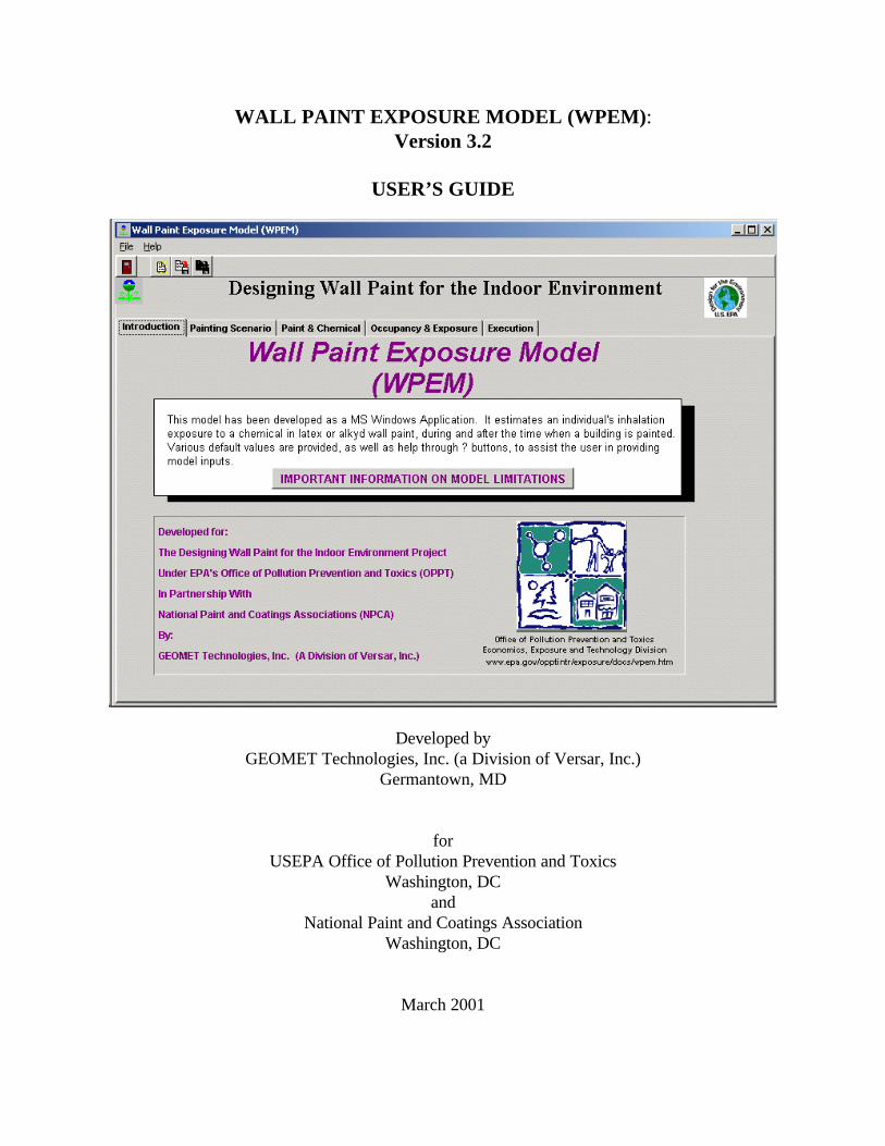
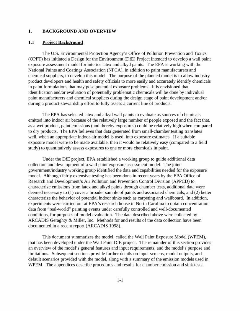
WPEM has been developed as a Windows 95/98 application. As noted in the IntroductionScreen for the model (Figure 1-1), it estimates an individual’s inhalation exposure to airborneconcentrations of a chemical released from latex or alkyd primer/paint, during and after the timewhen a building (residence, office, or standard box) is painted. The model requires certaininformation from the user in order to provide these estimates. User inputs are gathered in anorganized manner through a series of input screens called Painting Scenario, Paint & Chemical,and Occupancy & Exposure (see the tabs in Figure 1-1). Once these inputs have been provided,model calculations can be invoked through the Execution screen.
The following are the major types of information to be provided on each screen:
C Painting Scenario screen- building volume and airflow rates- percent of building painted- whether walls, ceilings, or both are painted- amount of paint used, painting rate, and resultant painting duration
C Paint & Chemical screen- type of paint and primer/paint density- properties of the chemical to be modeled, weight fraction in the primer/paint- chemical emissions model for primer and paint- indoor sink model (optional)
C Occupancy & Exposure screen- type/gender of exposed individual- individual’s location and breathing rate during the painting event- weekday and weekend activity patterns (locations, breathing rates)- number of painting events in lifetime- length of lifetime and body weight
C Execution screen- title of run and length of model run- results (exposure estimates) after execution- option to view/print a report summarizing inputs and outputs
The user is advised to proceed through these screens sequentially. Efforts have been madeto provide model defaults wherever possible, and to make certain calculations on behalf of theuser. Within each screen, areas where user inputs are required are shown in white. For example,
1-3
on the Painting Scenario screen the user must choose a residence, office building, or “standardbox,” and must indicate the number of coats applied for the primer and/or paint. Areas whereuser inputs are optional are shown in gray. For such areas, edit buttons enable the user tooverride default values that have been provided or calculated by the model. For example, on thePainting Scenario screen there is a default coverage of 400 square feet per gallon (equating to awet film thickness of 4 mil) for paint, but the user can override this value. Six default scenariosare provided with the WPEM software and can be accessed from the “File” “Open” toolbar inWPEM.
Figure 1-1. WPEM Introduction Screen.
1-4
Context-sensitive help for WPEM is provided through ? buttons. Each ? button is locatednear the input area to which it pertains. These buttons generally provide guidance for editingdefault selections or values provided with the model. In some cases, they also describe the basisfor a default value or the algorithm used by WPEM to calculate the value.
In addition, the following buttons provide background information on specific topic areas:
C IMPORTANT INFORMATION ON MODEL LIMITATIONS, located on theIntroduction screen;
C DESCRIPTION OF DEFAULT SCENARIOS, located on the Painting Scenarioscreen;
C DISPLAY CHEMICALS USED TO DEVELOP EMISSION MODELS, locatedon the Paint & Chemical screen; and
C MODEL LIMITATIONS, located on the Execution screen.
1.3 Model Purpose and Limitations
As noted in Section 1.1, the primary purpose of the model is to allow industry productdevelopers and health and safety officials to more easily and accurately identify chemicals in paintformulations that may pose potential exposure problems. Once the user has provided modelinputs as summarized in Section 1.2 and has executed the model, the resulting outputs can beused to assess inhalation exposure and associated risk for a chemical that is currently formulated,or is being considered for formulation, in primer and/or paint. The model provides both short-term and long-term exposure measures. Short-term measures include the highest instantaneous,15-minute-average, and 8-hour-average airborne concentration to which an individual is exposed,under the conditions represented by model inputs. Long-term measures include lifetime averagedaily dose (LADD) and lifetime average daily concentration (LADC).
The IMPORTANT INFORMATION ON MODEL LIMITATIONS button on theIntroduction screen (see Figure 1-1) describes some cautions to be considered when using themodel. For example, the model is designed to estimate indoor-air concentrations and associatedinhalation exposures for interior applications involving alkyd or latex primer/paint. The emissionalgorithms used in the model, and their relationship to chemical properties, are based on chambertests specific to interior paints. At present there is no basis for applying these algorithms to othertypes of products.
The model calculations are intended to represent the time series of indoor concentrationsfor a chemical, and exposure measures derived from those concentrations, that can be expectedwhen primer or paint is applied in an indoor environment. Although these calculations are basedon fundamental principles such as the conservation of chemical mass indoors, there are certainassumptions and/or limitations inherent in the model:
1-5
C The emission and sink models used in WPEM are derived from a limited number ofsmall-chamber tests, conducted at a fixed air exchange rate, a fixed loading ofwallboard, and a fixed product application rate for one type of application (roller).
C A single-chamber model is used when an entire building is painted; when part of abuilding is painted, a two-chamber model (painted and unpainted parts) is used.
C Within the modeled compartment(s), uniform mixing is assumed; no distinction ismade between airborne chemical concentrations in the applicator’s breathing zoneversus elsewhere in the compartment where paint is applied.
C Only one chemical can be modeled at a time; within a model run, it is not possibleto combine different primer/paint types (e.g., alkyd primer and latex paint), butsuch a combination can be modeled through separate model runs (see Section 4).
C The indoor-outdoor air exchange rate is treated as a constant (i.e., it cannot varyover time). Model defaults for the air exchange rate assume a closed-buildingcondition, as supporting data for other conditions (e.g., windows open or exhaustfans on) are limited.
C Dose estimates provided by the model are measures of potential inhaled dose (i.e.,100 percent uptake is assumed).
C The model has no capability for Monte Carlo simulation as a means of addressinguncertainty, but another model (MCCEM) developed for OPPT has this capability.
2-1
2. INPUT SCREENS
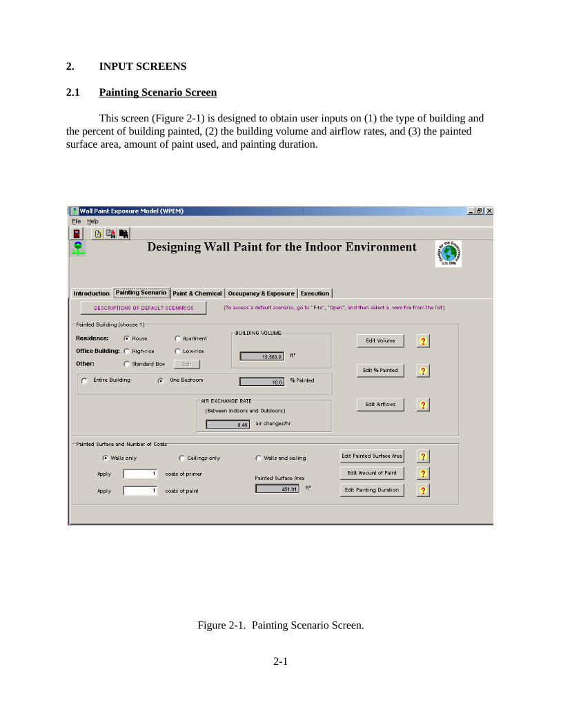
2.1 Painting Scenario Screen
This screen (Figure 2-1) is designed to obtain user inputs on (1) the type of building andthe percent of building painted, (2) the building volume and airflow rates, and (3) the paintedsurface area, amount of paint used, and painting duration.
Figure 2-1. Painting Scenario Screen.
2-2
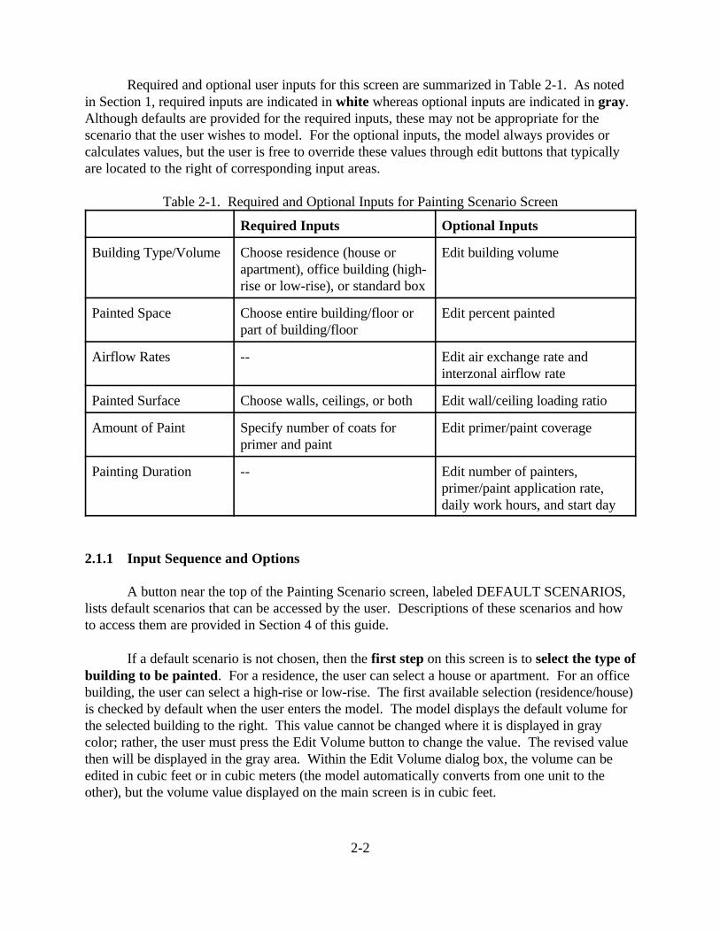
Required and optional user inputs for this screen are summarized in Table 2-1. As notedin Section 1, required inputs are indicated in white whereas optional inputs are indicated in gray. Although defaults are provided for the required inputs, these may not be appropriate for thescenario that the user wishes to model. For the optional inputs, the model always provides orcalculates values, but the user is free to override these values through edit buttons that typicallyare located to the right of corresponding input areas.
Table 2-1. Required and Optional Inputs for Painting Scenario Screen
Required Inputs Optional Inputs
Building Type/Volume Choose residence (house orapartment), office building (high-rise or low-rise), or standard box
Edit building volume
Painted Space Choose entire building/floor orpart of building/floor
Edit percent painted
Airflow Rates -- Edit air exchange rate andinterzonal airflow rate
Painted Surface Choose walls, ceilings, or both Edit wall/ceiling loading ratio
Amount of Paint Specify number of coats forprimer and paint
Edit primer/paint coverage
Painting Duration -- Edit number of painters,primer/paint application rate,daily work hours, and start day
2.1.1 Input Sequence and Options
A button near the top of the Painting Scenario screen, labeled DEFAULT SCENARIOS,lists default scenarios that can be accessed by the user. Descriptions of these scenarios and howto access them are provided in Section 4 of this guide.
If a default scenario is not chosen, then the first step on this screen is to select the type ofbuilding to be painted. For a residence, the user can select a house or apartment. For an officebuilding, the user can select a high-rise or low-rise. The first available selection (residence/house)is checked by default when the user enters the model. The model displays the default volume forthe selected building to the right. This value cannot be changed where it is displayed in graycolor; rather, the user must press the Edit Volume button to change the value. The revised valuethen will be displayed in the gray area. Within the Edit Volume dialog box, the volume can beedited in cubic feet or in cubic meters (the model automatically converts from one unit to theother), but the volume value displayed on the main screen is in cubic feet.
2-3
Another option for the type of painted building is a “standard box.” This choice allowsthe user to customize the scenario by supplying dimensions (length, width, and height) for thebuilding to be painted. When a standard box is selected, the building volume cannot be changedwith the Edit Volume button, but rather by editing the building dimensions.
The second step is to choose the building space to be painted. If residence/house isselected, for example, then the choices are entire building (100 percent) or one bedroom (10percent). Similar choices are provided for office building, (e.g., entire building or floor) andstandard box (entire building or part of building). The choice results in a model default value forpercent painted, which is displayed to the right in gray color. This value can be changed using theEdit % Painted button (unless entire building is selected for residence or standard box).
The third step (optional) is to specify an air exchange rate and interzonal airflow ratefor the selected building. The model provides default values keyed to the building types, and thedefault air exchange rate is displayed in gray color. The user can change this default value, aswell as the default value for the interzonal airflow rate, through the Edit Airflows button. Thereis one cautionary note here – changing the air exchange rate will cause the model to automaticallyuse a preset algorithm for the interzonal airflow rate; thus, if the user wishes to customize boththe air exchange rate and the interzonal airflow rate, then the air exchange rate should be changedfirst.
The fourth step is to choose the painted surface -- walls, ceilings, or both. The choiceleads to a model default value for the loading ratio (i.e., the ratio of surface area to volume). Thisvalue is not displayed on the main screen, but can be changed using the Edit Painted Surface Areabutton. The model uses the loading ratio to calculate the painted surface area, and displays thisvalue in gray color near the bottom-right portion of the main screen. The loading ratio can beedited either in ft2/ft3 or in m2/m3 (the model automatically converts from one unit to the other).
The fifth step is to choose the number of coats to be applied for primer and/or paint(one coat for each is shown by default). The user can elect to do painting only, for example, byentering zero coats for primer. Further details relating to the amount of primer/paint used areprovided through the Edit Amount of Paint button, where the coverage (ft2 or m2 per gallon) andassociated wet film thickness (mil, or 1/1000 inch) are displayed. For paint, the model provides adefault coverage of 400 ft2 per gallon (37.2 m2/gallon or 4.01 mil film thickness); the defaultcoverage for primer is half that of paint. These default values can be edited using any of the unitsprovided; the model calculates and displays the resultant amount of paint used (in gallons) withinthe dialog box. The amount of paint is not displayed on the main screen.
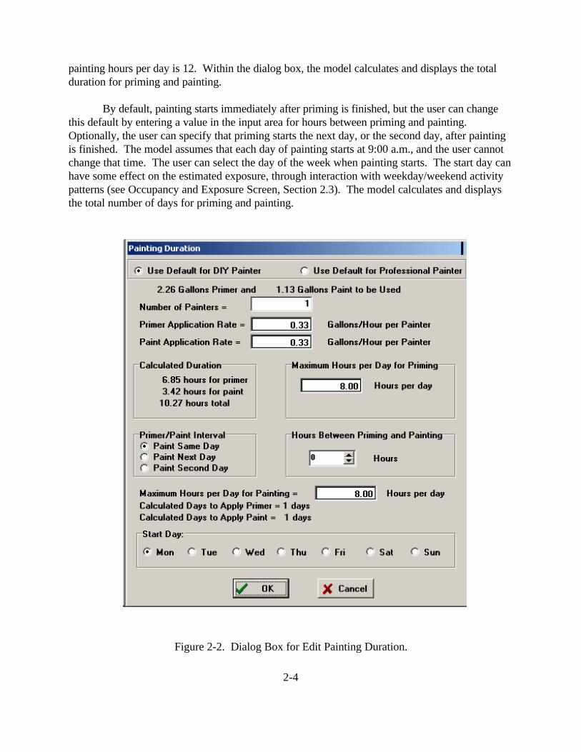
The final step for this screen is to determine the duration of the painting event, usingthe Edit Painting Duration button (see Figure 2-2). Within the associated dialog box, the user canchoose a default application rate for a do-it-yourself (DIY) or a professional painter and can editthe number of painters as well as the primer/paint application rates (gallons per hour) and themaximum priming/painting duration per day (hours). The maximum input value for priming or
2-4
painting hours per day is 12. Within the dialog box, the model calculates and displays the totalduration for priming and painting.
By default, painting starts immediately after priming is finished, but the user can changethis default by entering a value in the input area for hours between priming and painting. Optionally, the user can specify that priming starts the next day, or the second day, after paintingis finished. The model assumes that each day of painting starts at 9:00 a.m., and the user cannotchange that time. The user can select the day of the week when painting starts. The start day canhave some effect on the estimated exposure, through interaction with weekday/weekend activitypatterns (see Occupancy and Exposure Screen, Section 2.3). The model calculates and displaysthe total number of days for priming and painting.
Figure 2-2. Dialog Box for Edit Painting Duration.
2-5
2.1.2 Basis for Default Values
The basis for default values assigned on the Painting Scenario screen is summarized inTable 2-2. Some of the values, such as painting hours per day and start day for painting, arearbitrary selections intended to serve simply as “place holders” that the user can change. Severalof the values come from the Exposure Factors Handbook (USEPA 1997), Volume III, Chapter17 (Residence Characteristics). These include the default house volume (15,583 ft3 or 441.3 m3)and apartment volume (7,350 ft3 or 208.1m3), as well as the default residential air exchange rate of0.45 air changes per hour (ACH).
The default value for the interzonal airflow rate (IAR) for residences, in cubic meters perhour, is calculated by the model from the air exchange rate and house volume according to thefollowing equation:
IAR = (0.046 + 0.39*A)*V (2-1)
where A is the air exchange rate (inverse hours), and V is the building volume (cubic meters). The equation is an empirical relationship developed by Koontz and Rector (1995) from an analysisof residential volumes, air exchange rates and interzonal airflow rates. As described in thereferenced document, the relationship was developed through regression analysis, using airexchange rates and interzonal airflow rates (between the bedroom and the remainder of the house)that were measured in various field studies for using perfluorocarbon tracers (PFTs).
Table 2-2. Basis for Default Values on Painting Scenario Screen
Variable Basis for Default
Building Volume Exposure Factors Handbook for residencesProfessional judgment for office buildings
Percent Building Painted Arbitrary selection
Air Exchange Rate Exposure Factors Handbook for residencesPersily (1989) for office buildings
Interzonal Airflow Rate Koontz and Rector (1995) for residencesProfessional judgment for office buildings
Wall/Ceiling Loading Ratios Exposure Factors Handbook for residencesProfessional judgment for office buildings
Paint Coverage Label on paint containers
Paint Application Rate Household Solvent Products: A National Usage Survey(WESTAT 1987) for DIY paintersEstimating Guide, 19th Edition (PDCA 1998) forprofessional painters
Painting Hours Per Day Arbitrary selection
Start Day for Painting Arbitrary selection
2-6
Because available data are relatively scarce for office buildings, professional judgment wasused in developing certain defaults. For example, for the office-building interzonal airflow rate, itwas assumed that air communication between the painted and unpainted spaces occurs onlythrough the heating, ventilating, and air-conditioning (HVAC) system for the building. It wasfurther assumed that the internal recirculation of air through the HVAC system is equivalent toone air change per hour; that is, a volume of air equivalent to the total building volume iscirculated each hour. Given these assumptions, the interzonal airflow rate (IAR, in m3/hour) canbe calculated as follows:
IAR = building volume * % volume in painted area * % volume in unpainted area (2-2)
For example, if the building volume is 100,000 ft3 and the painted area is 10 percent of thatvolume, then the interzonal airflow rate is 100,000 * 0.1 * 0.9, or 9,000 ft3/hour.
In determining a default loading ratio for ceilings in office buildings, a ceiling height of 10feet was assumed. Because the volume is the product of the floor area times the ceiling height,the loading ratio for the ceiling (ceiling area/building volume) can be stated as:
ceiling area / (ceiling area * 10 ft) = 0.10 ft2/ft3, or 0.33 m2/m3 (2-3)
By comparison, the default ceiling loading ratio for residences (from the Exposure FactorsHandbook) is 0.13 ft2/ft3 (0.43 m2/m3).
To estimate a default loading ratio for walls in office buildings, a floor plan was laid outfor a building with a ceiling height of 10 feet. This floor plan was split equally into two spaces,one with 10 ft by 10 ft offices and associated hallways, and one with several larger areas thatwould contain cubicles. The resultant loading ratio for walls was estimated to be 0.25 ft2/ft3 (0.82m2/m3) , as compared to the default value of 0.29 ft2/ft3 (0.95 m2/m3) for residences.
For a standard box, the default air exchange rate, interzonal airflow rate, and loadingratios for walls and ceilings are the same as those for office buildings.
The default value for DIY paint application rate derives from an EPA-sponsored nationalusage survey of household solvent products. From that survey, the median amount of latex paintused is one gallon and the median duration of use is three hours, corresponding to an applicationrate of 0.33 gallons/hour. The default application rate for a professional painter derives from anestimating guide developed by the Painting and Decorating Contractors of America (PDCA). According to the guide, the labor production rate for painting is 337.5 ft2/hour (range of 325 to350 ft2/hour) for roller application. Given a paint coverage of 400 ft2/gallon, the labor productionrate equates to an application rate of 0.85 gallons/hour.
2-7
2.2 Paint & Chemical Screen
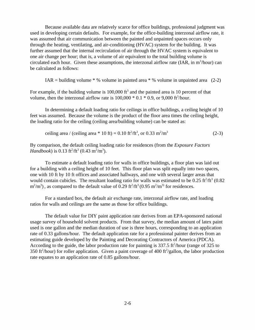
This screen (Figure 2-3) is designed to obtain user inputs on (1) the type of paint used andthe primer/paint density, (2) properties of the chemical under assessment, (3) the weight fractionof the chemical in primer and paint, (4) parameters of an emissions model for primer and paint,and (5) parameters for a sink model (or assumption of no indoor sinks).
Figure 2-3. Paint & Chemical Screen.
2-8
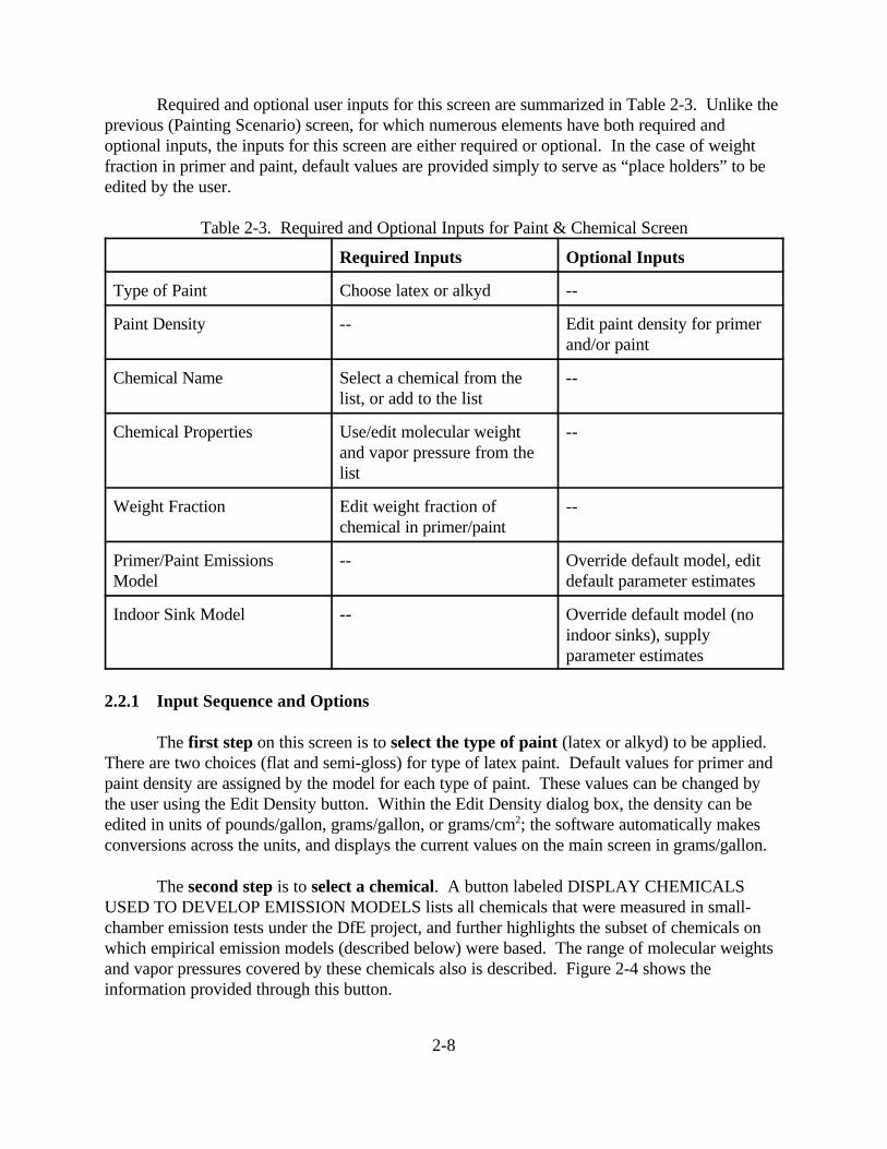
Required and optional user inputs for this screen are summarized in Table 2-3. Unlike theprevious (Painting Scenario) screen, for which numerous elements have both required andoptional inputs, the inputs for this screen are either required or optional. In the case of weightfraction in primer and paint, default values are provided simply to serve as “place holders” to beedited by the user.
Table 2-3. Required and Optional Inputs for Paint & Chemical Screen
Required Inputs Optional Inputs
Type of Paint Choose latex or alkyd --
Paint Density -- Edit paint density for primerand/or paint
Chemical Name Select a chemical from thelist, or add to the list
--
Chemical Properties Use/edit molecular weightand vapor pressure from thelist
--
Weight Fraction Edit weight fraction ofchemical in primer/paint
--
Primer/Paint EmissionsModel
-- Override default model, editdefault parameter estimates
Indoor Sink Model -- Override default model (noindoor sinks), supplyparameter estimates
2.2.1 Input Sequence and Options
The first step on this screen is to select the type of paint (latex or alkyd) to be applied. There are two choices (flat and semi-gloss) for type of latex paint. Default values for primer andpaint density are assigned by the model for each type of paint. These values can be changed bythe user using the Edit Density button. Within the Edit Density dialog box, the density can beedited in units of pounds/gallon, grams/gallon, or grams/cm2; the software automatically makesconversions across the units, and displays the current values on the main screen in grams/gallon.
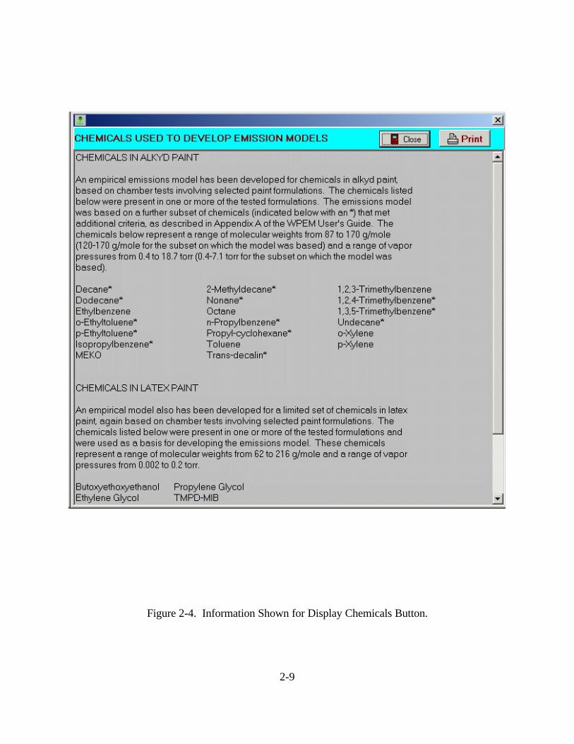
The second step is to select a chemical. A button labeled DISPLAY CHEMICALSUSED TO DEVELOP EMISSION MODELS lists all chemicals that were measured in small-chamber emission tests under the DfE project, and further highlights the subset of chemicals onwhich empirical emission models (described below) were based. The range of molecular weightsand vapor pressures covered by these chemicals also is described. Figure 2-4 shows theinformation provided through this button.
2-9
Figure 2-4. Information Shown for Display Chemicals Button.
2-10
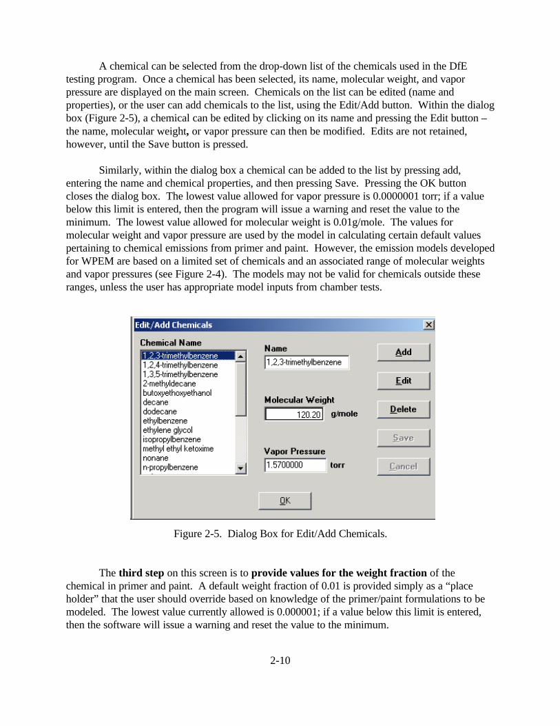
A chemical can be selected from the drop-down list of the chemicals used in the DfEtesting program. Once a chemical has been selected, its name, molecular weight, and vaporpressure are displayed on the main screen. Chemicals on the list can be edited (name andproperties), or the user can add chemicals to the list, using the Edit/Add button. Within the dialogbox (Figure 2-5), a chemical can be edited by clicking on its name and pressing the Edit button –the name, molecular weight, or vapor pressure can then be modified. Edits are not retained,however, until the Save button is pressed.
Similarly, within the dialog box a chemical can be added to the list by pressing add,entering the name and chemical properties, and then pressing Save. Pressing the OK buttoncloses the dialog box. The lowest value allowed for vapor pressure is 0.0000001 torr; if a valuebelow this limit is entered, then the program will issue a warning and reset the value to theminimum. The lowest value allowed for molecular weight is 0.01g/mole. The values formolecular weight and vapor pressure are used by the model in calculating certain default valuespertaining to chemical emissions from primer and paint. However, the emission models developedfor WPEM are based on a limited set of chemicals and an associated range of molecular weightsand vapor pressures (see Figure 2-4). The models may not be valid for chemicals outside theseranges, unless the user has appropriate model inputs from chamber tests.
Figure 2-5. Dialog Box for Edit/Add Chemicals.
The third step on this screen is to provide values for the weight fraction of thechemical in primer and paint. A default weight fraction of 0.01 is provided simply as a “placeholder” that the user should override based on knowledge of the primer/paint formulations to bemodeled. The lowest value currently allowed is 0.000001; if a value below this limit is entered,then the software will issue a warning and reset the value to the minimum.
2-11
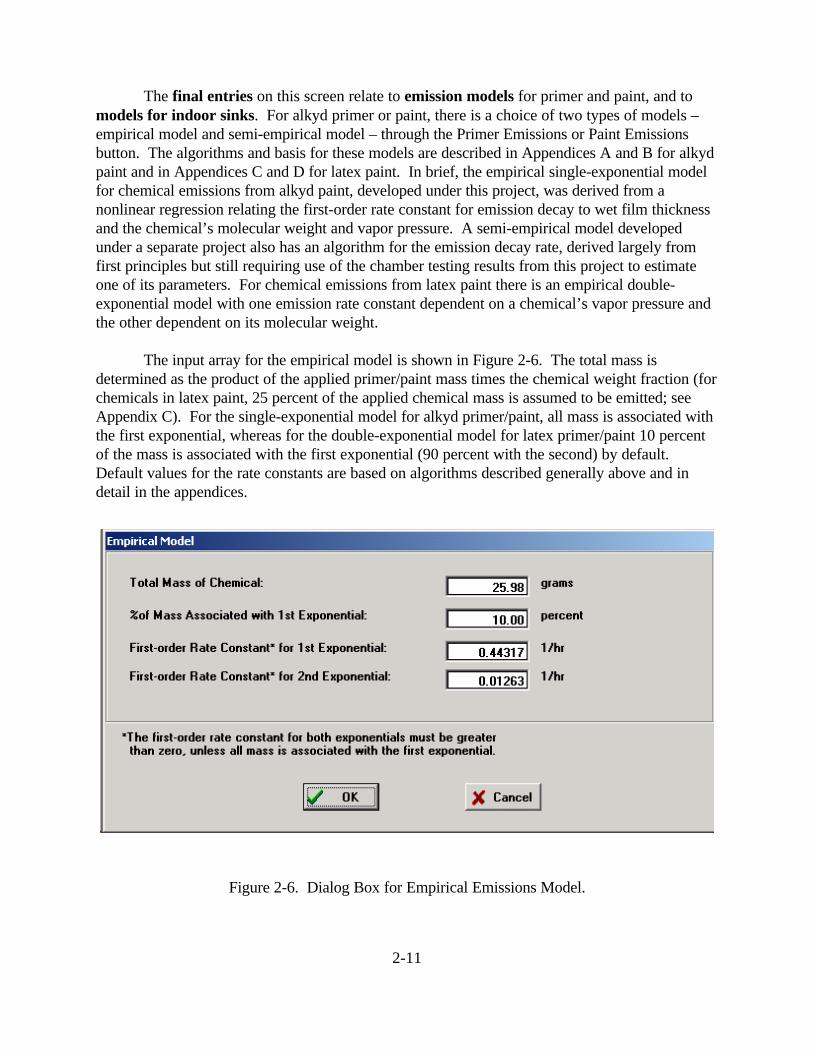
The final entries on this screen relate to emission models for primer and paint, and tomodels for indoor sinks. For alkyd primer or paint, there is a choice of two types of models –empirical model and semi-empirical model – through the Primer Emissions or Paint Emissionsbutton. The algorithms and basis for these models are described in Appendices A and B for alkydpaint and in Appendices C and D for latex paint. In brief, the empirical single-exponential modelfor chemical emissions from alkyd paint, developed under this project, was derived from anonlinear regression relating the first-order rate constant for emission decay to wet film thicknessand the chemical’s molecular weight and vapor pressure. A semi-empirical model developedunder a separate project also has an algorithm for the emission decay rate, derived largely fromfirst principles but still requiring use of the chamber testing results from this project to estimateone of its parameters. For chemical emissions from latex paint there is an empirical double-exponential model with one emission rate constant dependent on a chemical’s vapor pressure andthe other dependent on its molecular weight.
The input array for the empirical model is shown in Figure 2-6. The total mass isdetermined as the product of the applied primer/paint mass times the chemical weight fraction (forchemicals in latex paint, 25 percent of the applied chemical mass is assumed to be emitted; seeAppendix C). For the single-exponential model for alkyd primer/paint, all mass is associated withthe first exponential, whereas for the double-exponential model for latex primer/paint 10 percentof the mass is associated with the first exponential (90 percent with the second) by default. Default values for the rate constants are based on algorithms described generally above and indetail in the appendices.
Figure 2-6. Dialog Box for Empirical Emissions Model.
2-12
Default values for all parameters needed for the empirical model are supplied by theWPEM software. It is recommended that the user retain these defaults unless there are chemical-specific data (e.g., from small-chamber emission tests) that suggest more appropriate values.
Two types of indoor-sink models -- one-way sink and reversible sink – are availablethrough the Indoor Sinks button (the default is no indoor sinks). With a one-way sink, chemicalmass in the indoor air can move into the sink but can never exit it, whereas for a reversible sinkchemical mass can enter and leave the sink. The rate of mass entering the sink is governed inWPEM by an adsorption rate constant, and the rate of mass leaving the sink by a desorption rateconstant. Thus, for the one-way sink model, inputs are required for the area and adsorption ratefor each sink; for the reversible-sink model, inputs are required for a desorption rate as well. Theone-way sink model can be viewed as a special case of the reversible-sink model whereby alldesorption rates are zero.
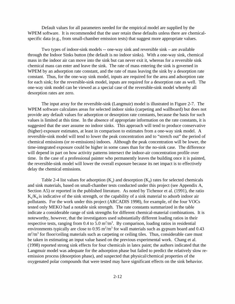
The input array for the reversible-sink (Langmuir) model is illustrated in Figure 2-7. TheWPEM software calculates areas for selected indoor sinks (carpeting and wallboard) but does notprovide any default values for adsorption or desorption rate constants, because the basis for suchvalues is limited at this time. In the absence of appropriate information on the rate constants, it issuggested that the user assume no indoor sinks. This approach will tend to produce conservative(higher) exposure estimates, at least in comparison to estimates from a one-way sink model. Areversible-sink model will tend to lower the peak concentration and to “stretch out” the period ofchemical emissions (or re-emissions) indoors. Although the peak concentration will be lower, thetime-integrated exposure could be higher in some cases than for the no-sink case. The differencewill depend in part on how activity patterns intersect the indoor-air concentration profile overtime. In the case of a professional painter who permanently leaves the building once it is painted,the reversible-sink model will lower the overall exposure because its net impact is to effectivelydelay the chemical emissions.
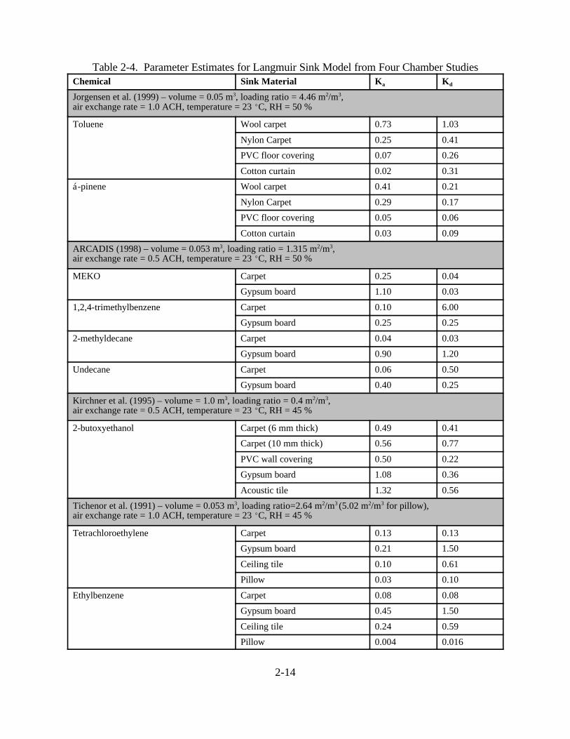
Table 2-4 list values for adsorption (Ka) and desorption (Kd) rates for selected chemicalsand sink materials, based on small-chamber tests conducted under this project (see Appendix A,Section A5) or reported in the published literature. As noted by Tichenor et al. (1991), the ratioKa/Kd is indicative of the sink strength, or the capability of a sink material to adsorb indoor airpollutants. For the work under this project (ARCADIS 1998), for example, of the four VOCstested only MEKO had a notable sink strength. The rate constants summarized in the tableindicate a considerable range of sink strengths for different chemical-material combinations. It isnoteworthy, however, that the investigators used substantially different loading ratios in theirrespective tests, ranging from 0.4 to 5.0 m2/m3. By comparison, loading ratios in residentialenvironments typically are close to 0.95 m2/m3 for wall materials such as gypsum board and 0.43m2/m3 for floor/ceiling materials such as carpeting or ceiling tiles. Thus, considerable care mustbe taken in estimating an input value based on the previous experimental work. Chang et al.(1998) reported strong sink effects for four chemicals in latex paint; the authors indicated that theLangmuir model was adequate for the adsorption phase but failed to predict the relatively slow re-emission process (desorption phase), and suspected that physical/chemical properties of theoxygenated polar compounds that were tested may have significant effects on the sink behavior.
2-13
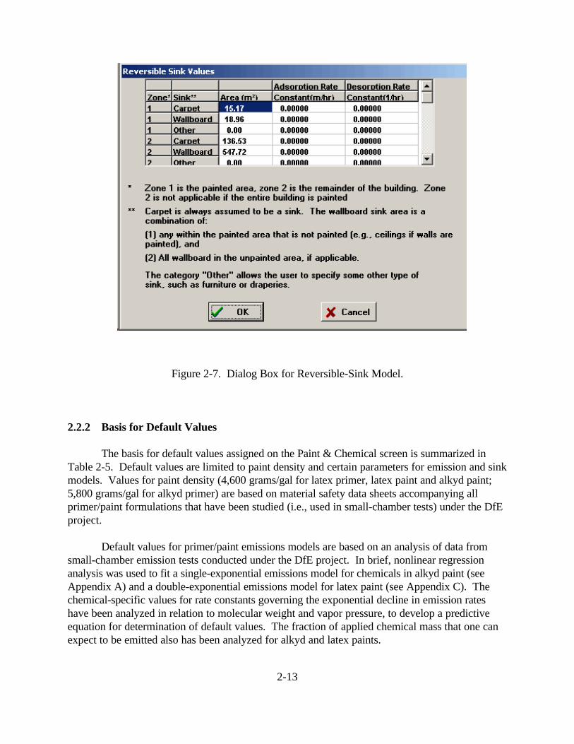
Figure 2-7. Dialog Box for Reversible-Sink Model.
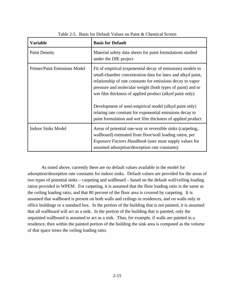
2.2.2 Basis for Default Values
The basis for default values assigned on the Paint & Chemical screen is summarized inTable 2-5. Default values are limited to paint density and certain parameters for emission and sinkmodels. Values for paint density (4,600 grams/gal for latex primer, latex paint and alkyd paint;5,800 grams/gal for alkyd primer) are based on material safety data sheets accompanying allprimer/paint formulations that have been studied (i.e., used in small-chamber tests) under the DfEproject.
Default values for primer/paint emissions models are based on an analysis of data fromsmall-chamber emission tests conducted under the DfE project. In brief, nonlinear regressionanalysis was used to fit a single-exponential emissions model for chemicals in alkyd paint (seeAppendix A) and a double-exponential emissions model for latex paint (see Appendix C). Thechemical-specific values for rate constants governing the exponential decline in emission rateshave been analyzed in relation to molecular weight and vapor pressure, to develop a predictiveequation for determination of default values. The fraction of applied chemical mass that one canexpect to be emitted also has been analyzed for alkyd and latex paints.
2-14
Table 2-4. Parameter Estimates for Langmuir Sink Model from Four Chamber StudiesChemical Sink Material Ka Kd
Jorgensen et al. (1999) – volume = 0.05 m3, loading ratio = 4.46 m2/m3, air exchange rate = 1.0 ACH, temperature = 23 EC, RH = 50 %
Toluene Wool carpet 0.73 1.03
Nylon Carpet 0.25 0.41
PVC floor covering 0.07 0.26
Cotton curtain 0.02 0.31
á-pinene Wool carpet 0.41 0.21
Nylon Carpet 0.29 0.17
PVC floor covering 0.05 0.06
Cotton curtain 0.03 0.09
ARCADIS (1998) – volume = 0.053 m3, loading ratio = 1.315 m2/m3,air exchange rate = 0.5 ACH, temperature = 23 EC, RH = 50 %
MEKO Carpet 0.25 0.04
Gypsum board 1.10 0.03
1,2,4-trimethylbenzene Carpet 0.10 6.00
Gypsum board 0.25 0.25
2-methyldecane Carpet 0.04 0.03
Gypsum board 0.90 1.20
Undecane Carpet 0.06 0.50
Gypsum board 0.40 0.25
Kirchner et al. (1995) – volume = 1.0 m3, loading ratio = 0.4 m2/m3,air exchange rate = 0.5 ACH, temperature = 23 EC, RH = 45 %
2-butoxyethanol Carpet (6 mm thick) 0.49 0.41
Carpet (10 mm thick) 0.56 0.77
PVC wall covering 0.50 0.22
Gypsum board 1.08 0.36
Acoustic tile 1.32 0.56
Tichenor et al. (1991) – volume = 0.053 m3, loading ratio=2.64 m2/m3 (5.02 m2/m3 for pillow),air exchange rate = 1.0 ACH, temperature = 23 EC, RH = 45 %
Tetrachloroethylene Carpet 0.13 0.13
Gypsum board 0.21 1.50
Ceiling tile 0.10 0.61
Pillow 0.03 0.10
Ethylbenzene Carpet 0.08 0.08
Gypsum board 0.45 1.50
Ceiling tile 0.24 0.59
Pillow 0.004 0.016
2-15
Table 2-5. Basis for Default Values on Paint & Chemical Screen
Variable Basis for Default
Paint Density Material safety data sheets for paint formulations studiedunder the DfE project
Primer/Paint Emissions Model Fit of empirical (exponential decay of emissions) models tosmall-chamber concentration data for latex and alkyd paint,relationship of rate constants for emissions decay to vaporpressure and molecular weight (both types of paint) and towet film thickness of applied product (alkyd paint only)
Development of semi-empirical model (alkyd paint only)relating rate constant for exponential emissions decay topaint formulation and wet film thickness of applied product
Indoor Sinks Model Areas of potential one-way or reversible sinks (carpeting,.wallboard) estimated from floor/wall loading ratios, perExposure Factors Handbook (user must supply values forassumed adsorption/desorption rate constants)
As noted above, currently there are no default values available in the model foradsorption/desorption rate constants for indoor sinks. Default values are provided for the areas oftwo types of potential sinks – carpeting and wallboard – based on the default wall/ceiling loadingratios provided in WPEM. For carpeting, it is assumed that the floor loading ratio is the same asthe ceiling loading ratio, and that 80 percent of the floor area is covered by carpeting. It isassumed that wallboard is present on both walls and ceilings in residences, and on walls only inoffice buildings or a standard box. In the portion of the building that is not painted, it is assumedthat all wallboard will act as a sink. In the portion of the building that is painted, only theunpainted wallboard is assumed to act as a sink. Thus, for example, if walls are painted in aresidence, then within the painted portion of the building the sink area is computed as the volumeof that space times the ceiling loading ratio.
2-16
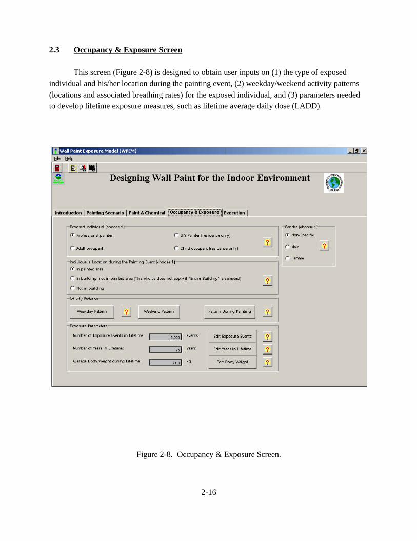
2.3 Occupancy & Exposure Screen
This screen (Figure 2-8) is designed to obtain user inputs on (1) the type of exposedindividual and his/her location during the painting event, (2) weekday/weekend activity patterns(locations and associated breathing rates) for the exposed individual, and (3) parameters neededto develop lifetime exposure measures, such as lifetime average daily dose (LADD).
Figure 2-8. Occupancy & Exposure Screen.
2-17
Required and optional user inputs for this screen are summarized in Table 2-6. Most ofthe inputs are optional, as the model provides many default choices or values here. The onlychoice required of the user is the type of exposed individual (professional painter by default). Once the exposed individual is selected, the model provides a default location during the paintingevent, which the user can override. Similarly, default values are provided for activity patterns,number of exposure events, years in lifetime, and body weight.
Table 2-6. Required and Optional Inputs for Occupancy & Exposure Screen
Required Inputs Optional Inputs
Exposed Individual Choose a type of exposedindividual
--
Gender -- Override default choice(non-specific gender)
Location during the PaintEvent
Choose a location (defaultvalue is linked to type ofexposed individual)
--
Activity Patterns -- Override default values fortime, location, or breathingrate for weekday/weekendpatterns (breathing rate onlyfor pattern during painting)
Number of Exposure Eventsin Lifetime
-- Override default values forevents per year and years ofexposure
Number of Years in Lifetime -- Override default value
Body Weight -- Override default value
2.3.1 Input Sequence and Options
The first step on this screen is to select the type of exposed individual. Differentdefault activity patterns and lifetime exposure events or years of life are provided in the model foreach of four types of exposed individuals – professional painter, do-it-yourself (DIY) painter,adult occupant, and child occupant. Two of these choices – DIY painter and child occupant – arenot valid if the user has specified on the Painting Scenario screen that an office building orstandard box is being painted.
2-18
The second step is to choose the gender of the exposed individual. The choice of gender(non-specific is the default) affects the default values supplied by WPEM for breathing rate, yearsin lifetime, and body weight.
The third step is to choose the individual’s location during the painting event, forwhich the model always provides a default that is tied to the type of exposed individual. Forexample, by default an adult or child occupant is assumed to be in the building, but not in thepainted area, during the painting event. The model will issue a warning if a professional or DIYpainter is not placed in the painted area, but will allow the user to make that choice.
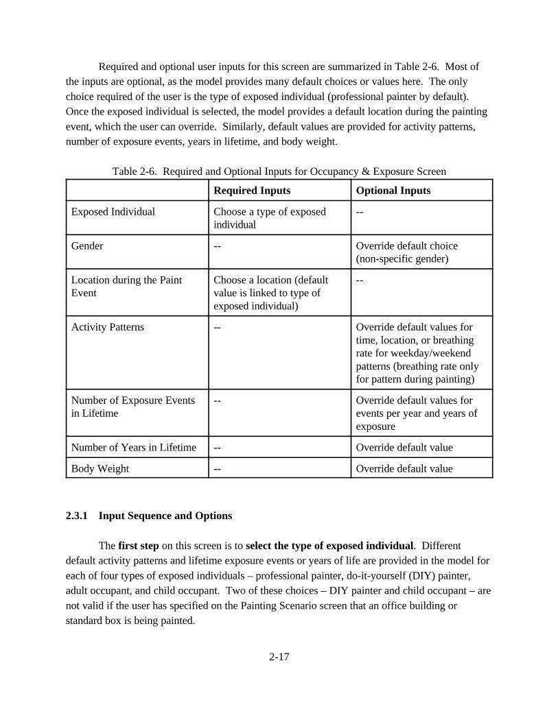
The fourth step (optional) is to edit the weekday/weekend activity patterns, oractivity patterns during the painting event, that already are provided by the model. Theweekday and weekend patterns (see Figure 2-9 for an example) have been developed to match thetypical amounts of daily time spent at home (in bedrooms and in the remainder of the house), atwork, and outdoors by the different types of individuals listed above, as reported in the ExposureFactors Handbook. The defaults should suffice for most applications.
Figure 2-9. Example Default Weekday Activity Pattern.
2-19
Items that can be edited for weekday/weekend patterns are the time of day when eachenvironment is entered (enter time), location (zone) at that time, and breathing rate. The entertime is input in separate cells for hour of the day (Hr) and minute with the hour (Min). The entryfor hour must be between 0 (midnight, or beginning of the day) and 23 (11 p.m.), and the entryfor minute must be between 0 and 59. The first enter time must be 0 Hr, 0 Min, and the usercannot edit that value. Another constraint is that the enter time for any given line must be laterthan the time for the line that precedes it. Exit times do not need to be entered, as the enter timefor the current line equates to the exit time for the previous line. The final entry is in effect untilthe end of the 24-hour day. For the example in Figure 2-9, the individual enters zone 1 (thepainted potion of the building) at midnight, enters zone 2 (the unpainted portion) at 7 a.m., leavesthe building (zone 0) at 8 a.m., returns to the building (zone 2) at 4 p.m. (hour 16), and enterszone 1 at 10 p.m. (hour 22).
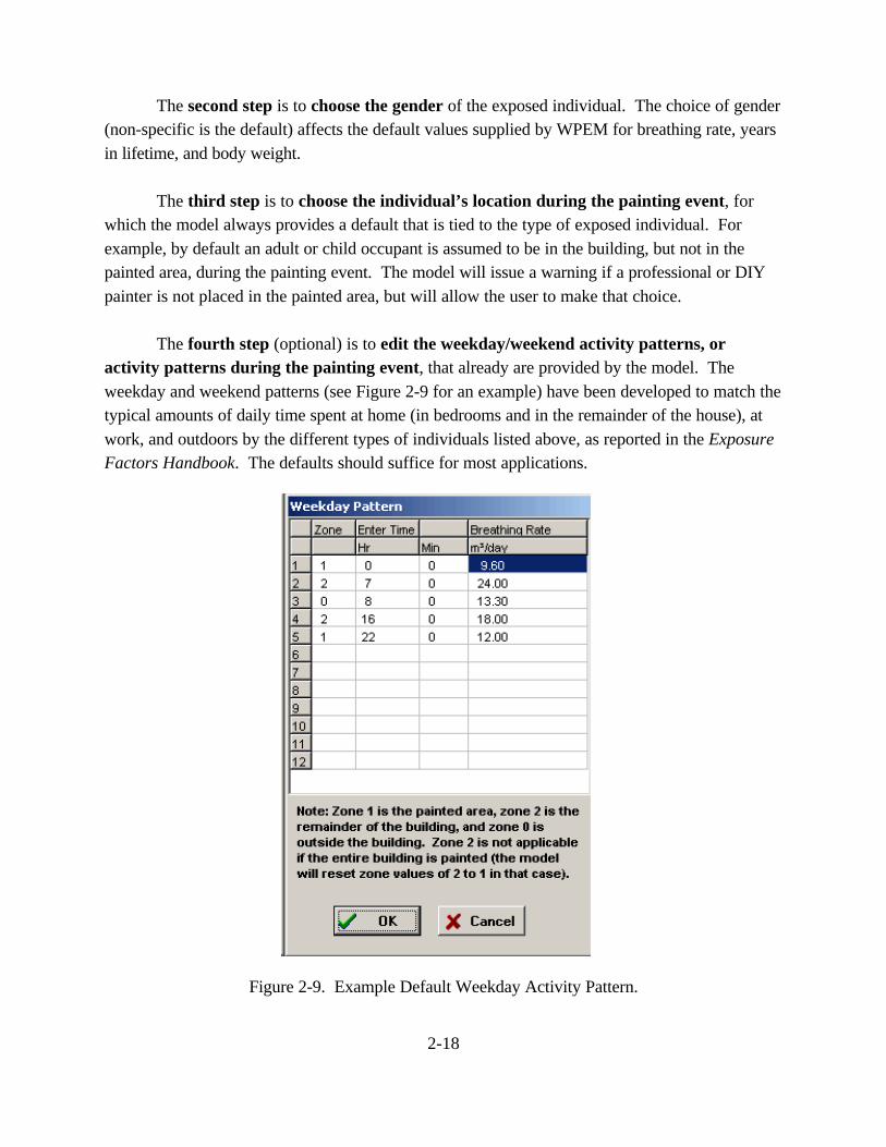
For the pattern during painting (Figure 2-10), only the breathing rate can be edited; allother inputs are determined by the model based on the user’s description of the priming/paintingevent on the Painting Scenario screen. This restriction prevents the user from entering a patternthat is inconsistent with the previously described painting event. Following the painting event, theindividual is placed in the location (zone) indicated by the weekday or weekend activity pattern(whichever applies) at the time when painting is finished.
Figure 2-10. Example Activity Pattern During Painting Determined by WPEM.
2-20
The final step (also optional) is to edit the exposure parameters – number of exposureevents in lifetime, number of years in lifetime, and body weight – through their associated editbuttons. A change to the default number of lifetime exposure events is accomplished by supplyingtwo values – exposure events per year and years of exposure. The default value for lifetimeexposure events is keyed to the type of exposed individual and to the type of building and percentpainted, from the Painting Scenario screen. For example, for a DIY painter, if the entire residenceis painted then one exposure event every 10 years is assumed by default. By comparison, if only abedroom is painted then one event per year is assumed. Further details on rules used by WPEMto calculate the default value for lifetime exposure events are provided in Section 2.3.2.
2.3.2 Basis for Default Values
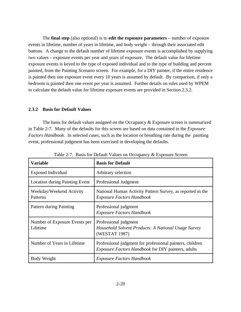
The basis for default values assigned on the Occupancy & Exposure screen is summarizedin Table 2-7. Many of the defaults for this screen are based on data contained in the Exposure
Factors Handbook. In selected cases, such as the location or breathing rate during the paintingevent, professional judgment has been exercised in developing the defaults.
Table 2-7. Basis for Default Values on Occupancy & Exposure Screen
Variable Basis for Default
Exposed Individual Arbitrary selection
Location during Painting Event Professional Judgment
Weekday/Weekend ActivityPatterns
National Human Activity Pattern Survey, as reported in theExposure Factors Handbook
Pattern during Painting Professional judgmentExposure Factors Handbook
Number of Exposure Events perLifetime
Professional judgmentHousehold Solvent Products: A National Usage Survey(WESTAT 1987)
Number of Years in Lifetime Professional judgment for professional painters, childrenExposure Factors Handbook for DIY painters, adults
Body Weight Exposure Factors Handbook
2-21
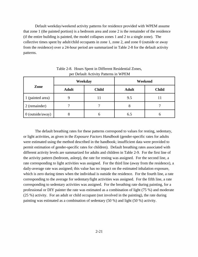
Default weekday/weekend activity patterns for residence provided with WPEM assumethat zone 1 (the painted portion) is a bedroom area and zone 2 is the remainder of the residence(if the entire building is painted, the model collapses zones 1 and 2 to a single zone). Thecollective times spent by adult/child occupants in zone 1, zone 2, and zone 0 (outside or awayfrom the residence) over a 24-hour period are summarized in Table 2-8 for the default activitypatterns.
Table 2-8. Hours Spent in Different Residential Zones, per Default Activity Patterns in WPEM
ZoneWeekday Weekend
Adult Child Adult Child
1 (painted area) 9 11 9.5 11
2 (remainder) 7 7 8 7
0 (outside/away) 8 6 6.5 6
The default breathing rates for these patterns correspond to values for resting, sedentary,or light activities, as given in the Exposure Factors Handbook (gender-specific rates for adultswere estimated using the method described in the handbook; insufficient data were provided topermit estimation of gender-specific rates for children). Default breathing rates associated withdifferent activity levels are summarized for adults and children in Table 2-9. For the first line ofthe activity pattern (bedroom, asleep), the rate for resting was assigned. For the second line, arate corresponding to light activities was assigned. For the third line (away from the residence), adaily-average rate was assigned; this value has no impact on the estimated inhalation exposure,which is zero during times when the individual is outside the residence. For the fourth line, a ratecorresponding to the average for sedentary/light activities was assigned. For the fifth line, a ratecorresponding to sedentary activities was assigned. For the breathing rate during painting, for aprofessional or DIY painter the rate was estimated as a combination of light (75 %) and moderate(25 %) activity. For an adult or child occupant (not involved in the painting), the rate duringpainting was estimated as a combination of sedentary (50 %) and light (50 %) activity.
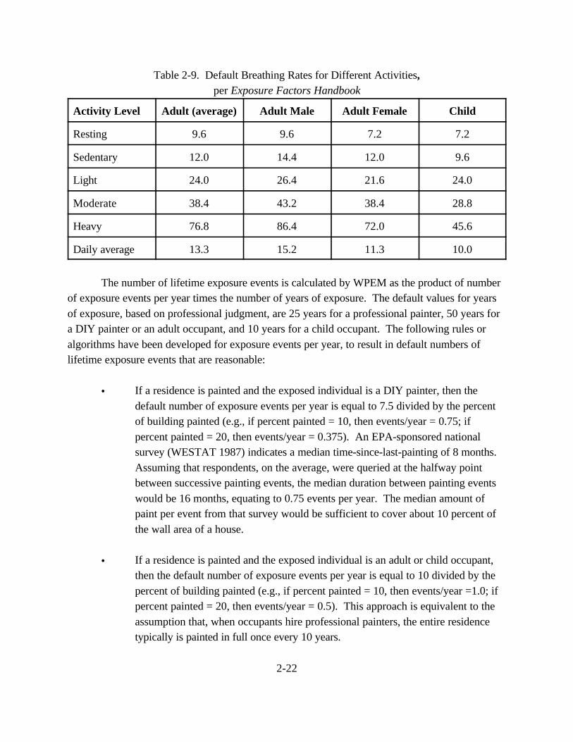
2-22
Table 2-9. Default Breathing Rates for Different Activities,per Exposure Factors Handbook
Activity Level Adult (average) Adult Male Adult Female Child
Resting 9.6 9.6 7.2 7.2
Sedentary 12.0 14.4 12.0 9.6
Light 24.0 26.4 21.6 24.0
Moderate 38.4 43.2 38.4 28.8
Heavy 76.8 86.4 72.0 45.6
Daily average 13.3 15.2 11.3 10.0
The number of lifetime exposure events is calculated by WPEM as the product of numberof exposure events per year times the number of years of exposure. The default values for yearsof exposure, based on professional judgment, are 25 years for a professional painter, 50 years fora DIY painter or an adult occupant, and 10 years for a child occupant. The following rules oralgorithms have been developed for exposure events per year, to result in default numbers oflifetime exposure events that are reasonable:
C If a residence is painted and the exposed individual is a DIY painter, then thedefault number of exposure events per year is equal to 7.5 divided by the percentof building painted (e.g., if percent painted = 10, then events/year = 0.75; ifpercent painted = 20, then events/year = 0.375). An EPA-sponsored nationalsurvey (WESTAT 1987) indicates a median time-since-last-painting of 8 months. Assuming that respondents, on the average, were queried at the halfway pointbetween successive painting events, the median duration between painting eventswould be 16 months, equating to 0.75 events per year. The median amount ofpaint per event from that survey would be sufficient to cover about 10 percent ofthe wall area of a house.
C If a residence is painted and the exposed individual is an adult or child occupant,then the default number of exposure events per year is equal to 10 divided by thepercent of building painted (e.g., if percent painted = 10, then events/year =1.0; ifpercent painted = 20, then events/year = 0.5). This approach is equivalent to theassumption that, when occupants hire professional painters, the entire residencetypically is painted in full once every 10 years.
2-23
C If an office or a standard box is painted and the exposed individual is an adultoccupant, then the number of exposure events per year is equal to 0.2, regardlessof the percent painted. This approach is equivalent to the assumption that theoffice building is painted once every five years.
C Regardless of type of building painted, if the exposed individual is a professionalpainter then the number of exposure events per year is equal to 1500 divided bythe total priming/painting duration (in hours), as determined on the PaintingScenario screen. With this approach, the painter spends 1500 hours per yearpainting (e.g., 50 weeks per year times 30 hours per week).
Gender-specific defaults taken from the Exposure Factors Handbook are provided foryears in lifetime. The default values for adults are 79 years for female, 72 years for male, and 75years for non-specific. For children the default is 10 years, regardless of gender. The default fora child does not correspond to length of lifetime per se, but rather to length of time as a child.
Gender-specific defaults taken from the Exposure Factors Handbook also are provided forbody weight. The default values for adults are 65.4 kg for female, 78.1 kg for male, and 71.8 kgfor non-specific. For children the default is 20.3 kg, regardless of gender. The body weight canbe edited in pounds or kg; the model automatically converts from one unit to the other, anddisplays the edited value in kg on the main screen.
2-24
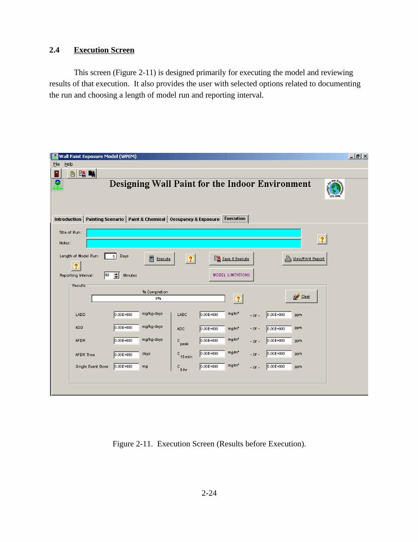
2.4 Execution Screen
This screen (Figure 2-11) is designed primarily for executing the model and reviewingresults of that execution. It also provides the user with selected options related to documentingthe run and choosing a length of model run and reporting interval.
Figure 2-11. Execution Screen (Results before Execution).
2-25
2.4.1 Input Sequence and Options
The first step on this screen is to provide optional entries for Title of Run and Notes. These entries enable the user to provide a general description of the run that is being made, alongwith some useful reminders such as input choices for one or more key parameters. If it is likelythat the full set of inputs for the run may need to be reviewed or perhaps updated at some futurepoint in time, then it is strongly recommended that the user save the inputs (see below).
The second step is to provide inputs for length of model run and reporting interval. Although the model provides a default value of 5 days for length of model run, this default isintended only as a “place holder,” to be edited by the user. The following are some useful tips fordetermining the length of model run:
C It takes a longer time for emissions from latex paint to decay than for emissionsfrom alkyd paint. The emissions from alkyd paint typically are “gone” within 24hours after painting is completed, unless a reversible-sink model is being used.
C A reversible-sink model for either latex or alkyd paint will tend to extend the timeduration during which chemical emissions (or re-emissions from the sink) arepresent.
C A professional painter leaves the building once it is painted and does not return. Thus, when a professional painter has been selected as the exposed individual, thelength of model run can be set equal to the total number of primer/painting days(or the total number of days plus one), as determined on the Painting Scenarioscreen.
C A model run that is too short can result in underestimaton of outputs such as singleevent dose or lifetime average daily dose. To ensure that a model run issufficiently long, initially select a number of days that is somewhat greater than thetotal number of priming/painting days, and note the resultant value for single eventdose. Next, select a length of model run that is a few days greater than the numberpreviously selected, rerun the model, and compare the value for single-event dosewith the previous result. When the dose value is no longer changing, or ischanging by a very small amount, the model run is sufficiently long.
The choice of reporting interval has no impact on the results displayed on this screen, as
the model uses an internal time step of 30 seconds for calculations in all cases. The reporting
2-26
interval does, however, affect the level of detail in a file generated by the model (see Section 3)that contains the time series of concentrations for each zone in the residence and for theconcentration to which the individual is exposed. The file can be easily imported into Excel, forexample, and plotted using the chart wizard. If the user wishes to examine this file and alsowishes to see greater time resolution than for the default reporting interval of 60 minutes, then ashorter interval such as 15 minutes or 5 minutes (as short as one minute) can be selected. Ashorter interval will result in greater time-related detail with a corresponding increase in the sizeof the file.
The third step is to execute the model. The user has the option of just executing themodel (Execute button) or first saving the inputs and then executing (Save & Execute button). The latter option is recommended as a general practice. Once inputs has been developed,documented and saved for a given run, they can readily be edited, for example, to make certainperturbations for examining various “what if” scenarios. Saving can be accomplished withoutexecuting through a Save button on the toolbar near the top of the screen. Standard Windowsoptions such as “Save” and “Save As” are available under File at the upper left of the screen. When a file is saved, WPEM always prompt for a name (with the current name displayed) so thatexisting files are not inadvertently overwritten.
Once the user has pressed Execute or Save & Execute, the Execute button changes to aStop button that can be used to abort the run. Such an action will save significant time only in theevent that the user has selected a relatively long length of model run (e.g., 15-20 days or greater).
Before executing the model, it may be useful to perform a quick review of inputs bypressing the View/Print Report button. As described in Section 3, the report both summarizesmodel inputs and presents model results. A button below the Save & Execute button, with a titleof MODEL LIMITATIONS, lists the limitations that were previously indicated in Section 1.3 ofthis guide. Following execution, the model results can be reset to zero if desired using the Clearbutton to the right of the % completion bar in the lower half of the screen.
2.4.2 Modeling Approach and Calculations
Indoor-air concentrations in one or two zones are predicted in WPEM by implementing adeterministic, mass-balance equation. The modeled concentration in each zone is a function of thetime-varying emission rate in one or more zone, the zone volumes, the airflow rates among zonesand between each zone and outdoors, losses to indoor sinks, and (if a reversible sink model isused) re-emissions from indoor sinks.
2-27
Consumer products such as paints that are applied to surfaces are best represented by anincremental source model. This model assumes a constant application rate over time, coupledwith an emission rate for each instantaneously applied segment that declines exponentially. Themathematical expression for the total emission rate resulting from the combination of constantapplication rate and exponential emission rate for each applied segment has been developed byEvans (1994).
The model requires the conservation of pollutant mass as well as the conservation of airmass. WPEM uses a set of differential equations whereby the time-varying concentration in eachzone is a function of the rate of pollutant loss and gain for that zone. These relationships can beexpressed as follows:
Pollutant Mass Balance
(Change in Pollutant Mass) / (Change in Time) = Production ± Transport - Removal ± Reactions
Neglecting reactions:
(d Mass) / (dt) = 3 Sources + 3 Mass in - 3 Mass out ± 3 Sinks (2-4)
Or:
(Vi dCi) / (dt) = 3 Sources + 3 Cj*Qji - 3 Ci*Qij ± 3 Sinks (2-5)
where C refers to an air concentration, Q refers to a flow rate, i and j refer to zones (there are upto two indoor zones plus outdoors), and the ± for sinks accounts for the possibility that they maybe reversible.
Air Mass Balance
Flows into a zone = Flows out of a zoneOr:
3 Qji = 3 Qij (2-6)
where Q, i and j are defined as above. The flow rates are input as constants. The pollutant massbalance is used in conjunction with the flow rates to predict the time-varying pollutantconcentration in each indoor zone.
2-28
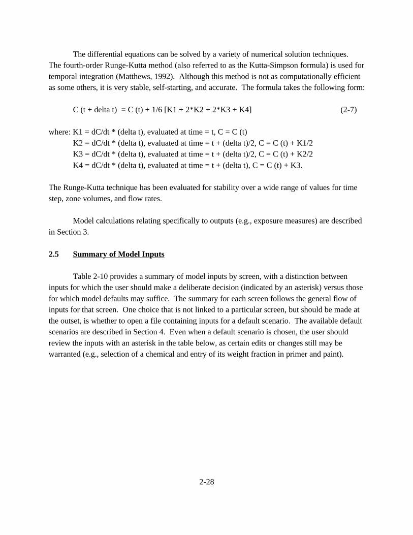
The differential equations can be solved by a variety of numerical solution techniques. The fourth-order Runge-Kutta method (also referred to as the Kutta-Simpson formula) is used fortemporal integration (Matthews, 1992). Although this method is not as computationally efficientas some others, it is very stable, self-starting, and accurate. The formula takes the following form:
C (t + delta t) = C (t) + 1/6 [K1 + 2*K2 + 2*K3 + K4] (2-7)
where: K1 = dC/dt * (delta t), evaluated at time = t, C = C (t)K2 = dC/dt * (delta t), evaluated at time = t + (delta t)/2, C = C (t) + K1/2K3 = dC/dt * (delta t), evaluated at time = t + (delta t)/2, C = C (t) + K2/2K4 = dC/dt * (delta t), evaluated at time = t + (delta t), C = C (t) + K3.
The Runge-Kutta technique has been evaluated for stability over a wide range of values for timestep, zone volumes, and flow rates.
Model calculations relating specifically to outputs (e.g., exposure measures) are describedin Section 3.
2.5 Summary of Model Inputs
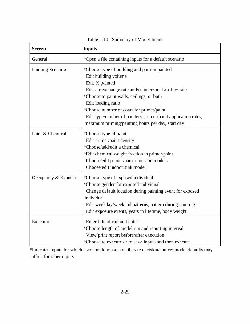
Table 2-10 provides a summary of model inputs by screen, with a distinction betweeninputs for which the user should make a deliberate decision (indicated by an asterisk) versus thosefor which model defaults may suffice. The summary for each screen follows the general flow ofinputs for that screen. One choice that is not linked to a particular screen, but should be made atthe outset, is whether to open a file containing inputs for a default scenario. The available defaultscenarios are described in Section 4. Even when a default scenario is chosen, the user shouldreview the inputs with an asterisk in the table below, as certain edits or changes still may bewarranted (e.g., selection of a chemical and entry of its weight fraction in primer and paint).
2-29
Table 2-10. Summary of Model Inputs
Screen Inputs
General *Open a file containing inputs for a default scenario
Painting Scenario *Choose type of building and portion painted Edit building volume Edit % painted Edit air exchange rate and/or interzonal airflow rate*Choose to paint walls, ceilings, or both Edit loading ratio*Choose number of coats for primer/paint Edit type/number of painters, primer/paint application rates, maximum priming/painting hours per day, start day
Paint & Chemical *Choose type of paint Edit primer/paint density*Choose/add/edit a chemical*Edit chemical weight fraction in primer/paint Choose/edit primer/paint emission models Choose/edit indoor sink model
Occupancy & Exposure *Choose type of exposed individual*Choose gender for exposed individual Change default location during painting event for exposed individual Edit weekday/weekend patterns, pattern during painting Edit exposure events, years in lifetime, body weight
Execution Enter title of run and notes*Choose length of model run and reporting interval View/print report before/after execution*Choose to execute or to save inputs and then execute
*Indicates inputs for which user should make a deliberate decision/choice; model defaults may suffice for other inputs.
3-1
3. MODEL RESULTS AND OUTPUTS
3.1 Exposure Estimates
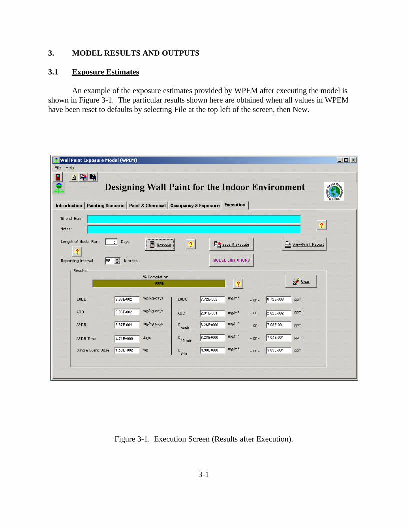
An example of the exposure estimates provided by WPEM after executing the model isshown in Figure 3-1. The particular results shown here are obtained when all values in WPEMhave been reset to defaults by selecting File at the top left of the screen, then New.
Figure 3-1. Execution Screen (Results after Execution).
3-2
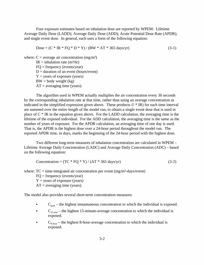
Four exposure estimates based on inhalation dose are reported by WPEM: LifetimeAverage Daily Dose (LADD); Average Daily Dose (ADD); Acute Potential Dose Rate (APDR);and single event dose. In general, each uses a form of the following equation:
Dose = (C * IR * FQ * D * Y) / (BW * AT * 365 days/yr) (3-1)
where: C = average air concentration (mg/m³)IR = inhalation rate (m³/hr)FQ = frequency (events/year)D = duration of an event (hours/event)Y = years of exposure (years)BW = body weight (kg)AT = averaging time (years).
The algorithm used in WPEM actually multiplies the air concentration every 30 secondsby the corresponding inhalation rate at that time, rather than using an average concentration asindicated in the simplified expression given above. These products © * IR) for each time intervalare summed over the entire length of the model run, to obtain a single event dose that is used inplace of C * IR in the equation given above. For the LADD calculation, the averaging time is thelifetime of the exposed individual. For the ADD calculation, the averaging time is the same as thenumber of years of exposure. For the APDR calculation, an averaging time of one day is used. That is, the APDR is the highest dose over a 24-hour period throughout the model run. Thereported APDR time, in days, marks the beginning of the 24-hour period with the highest dose.
Two different long-term measures of inhalation concentration are calculated in WPEM –Lifetime Average Daily Concentration (LADC) and Average Daily Concentration (ADC) – basedon the following equation:
Concentration = (TC * FQ * Y) / (AT * 365 days/yr) (3-2)
where: TC = time-integrated air concentration per event (mg/m³-days/event)FQ = frequency (events/year)Y = years of exposure (years)AT = averaging time (years).
The model also provides several short-term concentration measures:
C Cpeak – the highest instantaneous concentration to which the individual is exposed.
C C15-min – the highest 15-minute-average concentration to which the individual isexposed.
C C8-hour – the highest 8-hour-average concentration to which the individual isexposed.
3-3
The calculation engine for WPEM currently has no constraint relating to the saturationconcentration in air for the chemical that is modeled.
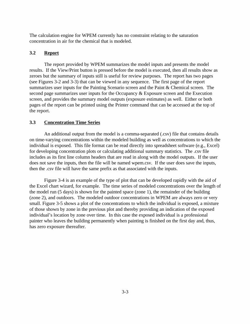
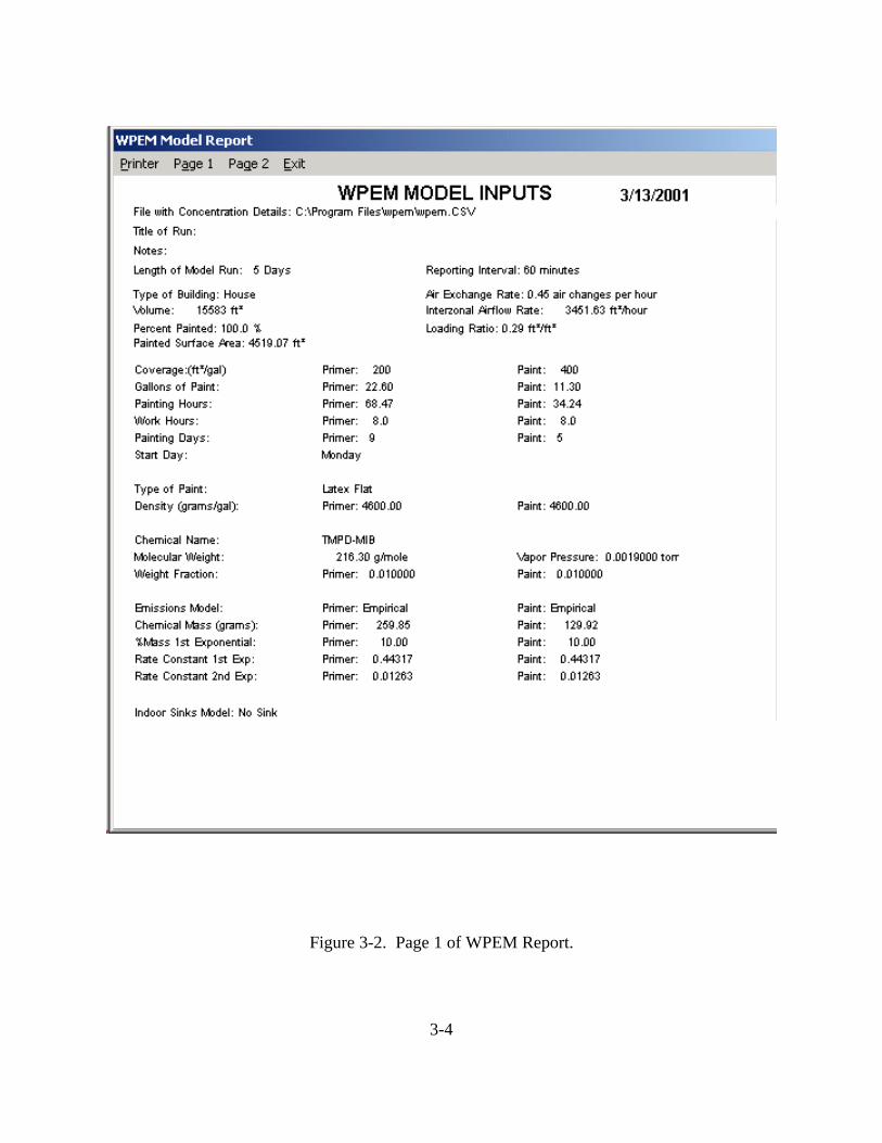
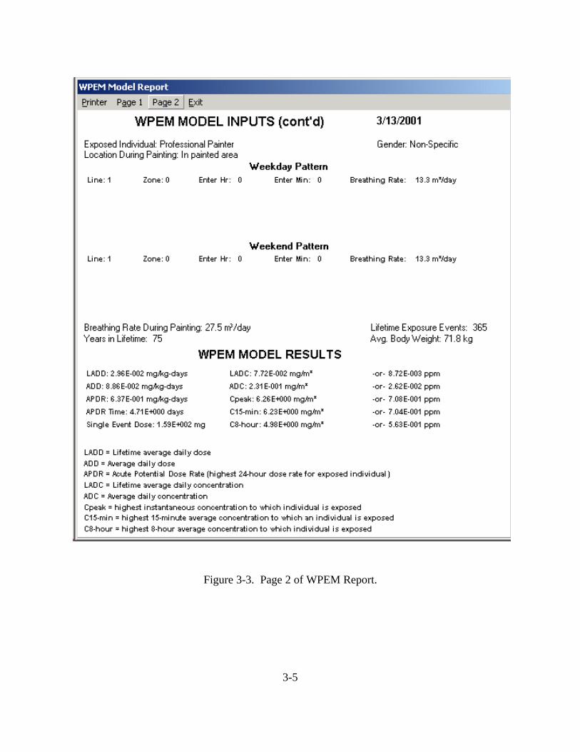
3.2 Report
The report provided by WPEM summarizes the model inputs and presents the modelresults. If the View/Print button is pressed before the model is executed, then all results show aszeroes but the summary of inputs still is useful for review purposes. The report has two pages(see Figures 3-2 and 3-3) that can be viewed in any sequence. The first page of the reportsummarizes user inputs for the Painting Scenario screen and the Paint & Chemical screen. Thesecond page summarizes user inputs for the Occupancy & Exposure screen and the Executionscreen, and provides the summary model outputs (exposure estimates) as well. Either or bothpages of the report can be printed using the Printer command that can be accessed at the top ofthe report.
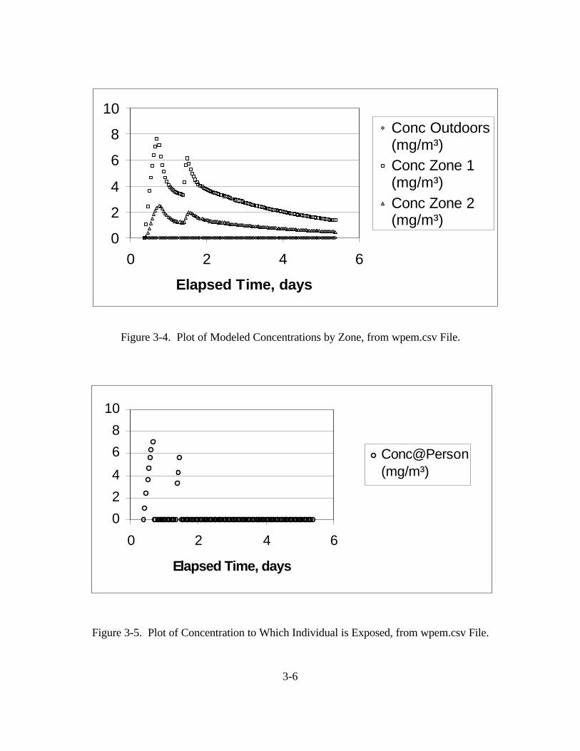
3.3 Concentration Time Series
An additional output from the model is a comma-separated (.csv) file that contains detailson time-varying concentrations within the modeled building as well as concentrations to which theindividual is exposed. This file format can be read directly into spreadsheet software (e.g., Excel)for developing concentration plots or calculating additional summary statistics. The .csv fileincludes as its first line column headers that are read in along with the model outputs. If the userdoes not save the inputs, then the file will be named wpem.csv. If the user does save the inputs,then the .csv file will have the same prefix as that associated with the inputs.
Figure 3-4 is an example of the type of plot that can be developed rapidly with the aid ofthe Excel chart wizard, for example. The time series of modeled concentrations over the length ofthe model run (5 days) is shown for the painted space (zone 1), the remainder of the building(zone 2), and outdoors. The modeled outdoor concentrations in WPEM are always zero or verysmall. Figure 3-5 shows a plot of the concentrations to which the individual is exposed, a mixtureof those shown by zone in the previous plot and thereby providing an indication of the exposedindividual’s location by zone over time. In this case the exposed individual is a professionalpainter who leaves the building permanently when painting is finished on the first day and, thus,has zero exposure thereafter.
3-4
Figure 3-2. Page 1 of WPEM Report.
3-5
Figure 3-3. Page 2 of WPEM Report.
3-6
0
2
4
6
8
10
0 2 4 6
Elapsed Time, days
Conc Outdoors(mg/m³)Conc Zone 1(mg/m³)Conc Zone 2(mg/m³)
0
2
4
6
8
10
0 2 4 6
Elapsed Time, days
Conc@Person(mg/m³)
Figure 3-4. Plot of Modeled Concentrations by Zone, from wpem.csv File.
Figure 3-5. Plot of Concentration to Which Individual is Exposed, from wpem.csv File.
4-1
4. DEFAULT SCENARIOS AND APPLICATION TIPS
4.1 Default Scenarios
A button near the top of the Painting Scenario screen, labeled DEFAULT SCENARIOS,lists six default scenarios that can be accessed by the user:
C RESDIY – A do-it-yourself (DIY) painter is exposed to a chemical in paint whilepainting the bedroom of a house.
C RESADULT – An adult located in the non-painted part of the house is exposed toa chemical in paint while a bedroom is painted by a professional painter.
C RESCHILD – A child located in the non-painted part of the house is exposed to achemical in paint while a bedroom is painted by a professional painter.
C RESPROF – Two professional painters are exposed to a chemical in paint whilepainting an entire apartment.
C OFFADULT – An office worker is exposed to a chemical in paint after an entirefloor of a low-rise office building is painted by ten professionals over a weekend.
C OFFPROF – Ten professional painters are exposed to a chemical in paint whilepainting an entire floor of a low-rise office building over a weekend.
The name associated with each scenario refers to a file that can be loaded to access thatscenario. Such files, provided with the model, are located in the directory from which WPEM isexecuted and have an extension of .wem. For example, to access the scenario called RESDIY,the user can open the file named resdiy.wem, using the “Open a File” button on the toolbar nearthe top of the screen. Alternatively, one can click on File at the top left of the screen, then Open,to access the files with default scenarios.
Each file contains defaults for entries such as the type and percent of building painted, theamount of primer and paint applied, the application rate and painting duration, the type ofexposed individual and location during the painting event, and the number of lifetime exposureevents. There are certain selections that are common across the default scenarios, such aspainting of walls only, selection of latex flat paint, selection of TMPD-MIB (texanol) as thechemical, and selection of non-specific gender for the exposed individual. These and other defaultentries should be reviewed by the user, and changed as needed using appropriate edit buttons,before executing the model.
Table 4-1 summarizes input values used for each of the default scenarios. Exposuredescriptors for each scenario follow the table (see Section 4.2). Some application tips areprovided in Section 4.3.
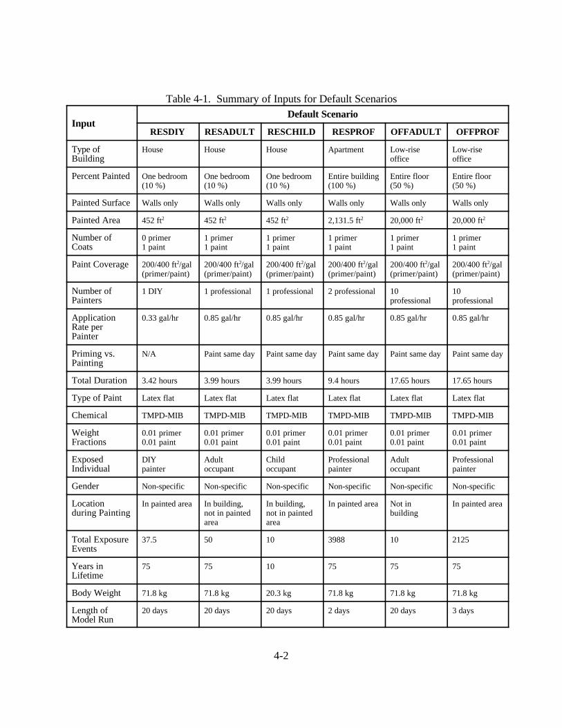
4-2
Table 4-1. Summary of Inputs for Default Scenarios
InputDefault Scenario
RESDIY RESADULT RESCHILD RESPROF OFFADULT OFFPROF
Type ofBuilding
House House House Apartment Low-riseoffice
Low-riseoffice
Percent Painted One bedroom(10 %)
One bedroom(10 %)
One bedroom(10 %)
Entire building(100 %)
Entire floor(50 %)
Entire floor(50 %)
Painted Surface Walls only Walls only Walls only Walls only Walls only Walls only
Painted Area 452 ft2 452 ft2 452 ft2 2,131.5 ft2 20,000 ft2 20,000 ft2
Number ofCoats
0 primer1 paint
1 primer1 paint
1 primer1 paint
1 primer1 paint
1 primer1 paint
1 primer1 paint
Paint Coverage 200/400 ft2/gal(primer/paint)
200/400 ft2/gal(primer/paint)
200/400 ft2/gal(primer/paint)
200/400 ft2/gal(primer/paint)
200/400 ft2/gal(primer/paint)
200/400 ft2/gal(primer/paint)
Number ofPainters
1 DIY 1 professional 1 professional 2 professional 10professional
10professional
ApplicationRate perPainter
0.33 gal/hr 0.85 gal/hr 0.85 gal/hr 0.85 gal/hr 0.85 gal/hr 0.85 gal/hr
Priming vs.Painting
N/A Paint same day Paint same day Paint same day Paint same day Paint same day
Total Duration 3.42 hours 3.99 hours 3.99 hours 9.4 hours 17.65 hours 17.65 hours
Type of Paint Latex flat Latex flat Latex flat Latex flat Latex flat Latex flat
Chemical TMPD-MIB TMPD-MIB TMPD-MIB TMPD-MIB TMPD-MIB TMPD-MIB
WeightFractions
0.01 primer0.01 paint
0.01 primer0.01 paint
0.01 primer0.01 paint
0.01 primer0.01 paint
0.01 primer0.01 paint
0.01 primer0.01 paint
ExposedIndividual
DIYpainter
Adultoccupant
Childoccupant
Professionalpainter
Adultoccupant
Professionalpainter
Gender Non-specific Non-specific Non-specific Non-specific Non-specific Non-specific
Locationduring Painting
In painted area In building,not in paintedarea
In building,not in paintedarea
In painted area Not inbuilding
In painted area
Total ExposureEvents
37.5 50 10 3988 10 2125
Years inLifetime
75 75 10 75 75 75
Body Weight 71.8 kg 71.8 kg 20.3 kg 71.8 kg 71.8 kg 71.8 kg
Length ofModel Run
20 days 20 days 20 days 2 days 20 days 3 days
4-3
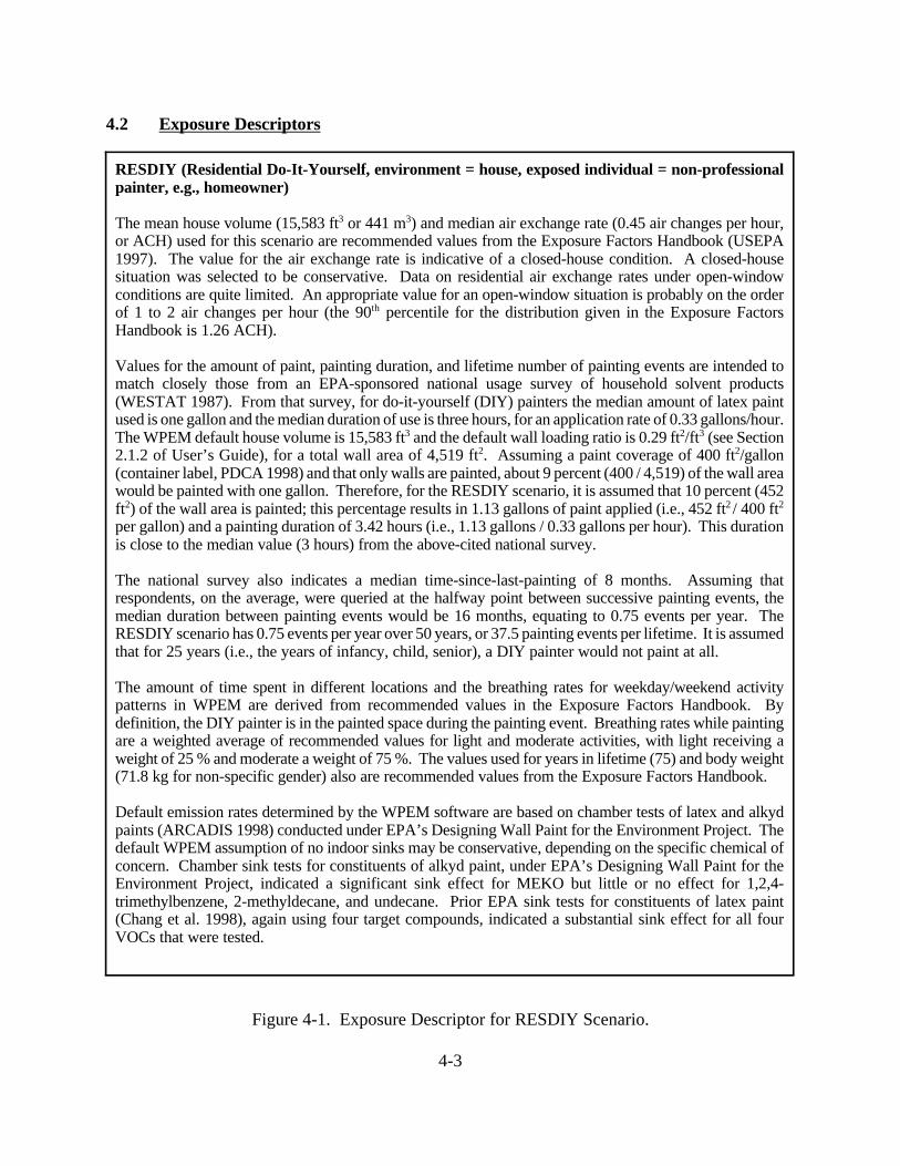
RESDIY (Residential Do-It-Yourself, environment = house, exposed individual = non-professionalpainter, e.g., homeowner)
The mean house volume (15,583 ft3 or 441 m3) and median air exchange rate (0.45 air changes per hour,or ACH) used for this scenario are recommended values from the Exposure Factors Handbook (USEPA1997). The value for the air exchange rate is indicative of a closed-house condition. A closed-housesituation was selected to be conservative. Data on residential air exchange rates under open-windowconditions are quite limited. An appropriate value for an open-window situation is probably on the orderof 1 to 2 air changes per hour (the 90th percentile for the distribution given in the Exposure FactorsHandbook is 1.26 ACH).
Values for the amount of paint, painting duration, and lifetime number of painting events are intended tomatch closely those from an EPA-sponsored national usage survey of household solvent products(WESTAT 1987). From that survey, for do-it-yourself (DIY) painters the median amount of latex paintused is one gallon and the median duration of use is three hours, for an application rate of 0.33 gallons/hour.The WPEM default house volume is 15,583 ft3 and the default wall loading ratio is 0.29 ft2/ft3 (see Section2.1.2 of User’s Guide), for a total wall area of 4,519 ft2. Assuming a paint coverage of 400 ft2/gallon(container label, PDCA 1998) and that only walls are painted, about 9 percent (400 / 4,519) of the wall areawould be painted with one gallon. Therefore, for the RESDIY scenario, it is assumed that 10 percent (452ft2) of the wall area is painted; this percentage results in 1.13 gallons of paint applied (i.e., 452 ft2 / 400 ft2
per gallon) and a painting duration of 3.42 hours (i.e., 1.13 gallons / 0.33 gallons per hour). This durationis close to the median value (3 hours) from the above-cited national survey.
The national survey also indicates a median time-since-last-painting of 8 months. Assuming thatrespondents, on the average, were queried at the halfway point between successive painting events, themedian duration between painting events would be 16 months, equating to 0.75 events per year. TheRESDIY scenario has 0.75 events per year over 50 years, or 37.5 painting events per lifetime. It is assumedthat for 25 years (i.e., the years of infancy, child, senior), a DIY painter would not paint at all.
The amount of time spent in different locations and the breathing rates for weekday/weekend activitypatterns in WPEM are derived from recommended values in the Exposure Factors Handbook. Bydefinition, the DIY painter is in the painted space during the painting event. Breathing rates while paintingare a weighted average of recommended values for light and moderate activities, with light receiving aweight of 25 % and moderate a weight of 75 %. The values used for years in lifetime (75) and body weight(71.8 kg for non-specific gender) also are recommended values from the Exposure Factors Handbook.
Default emission rates determined by the WPEM software are based on chamber tests of latex and alkydpaints (ARCADIS 1998) conducted under EPA’s Designing Wall Paint for the Environment Project. Thedefault WPEM assumption of no indoor sinks may be conservative, depending on the specific chemical ofconcern. Chamber sink tests for constituents of alkyd paint, under EPA’s Designing Wall Paint for theEnvironment Project, indicated a significant sink effect for MEKO but little or no effect for 1,2,4-trimethylbenzene, 2-methyldecane, and undecane. Prior EPA sink tests for constituents of latex paint(Chang et al. 1998), again using four target compounds, indicated a substantial sink effect for all fourVOCs that were tested.
4.2 Exposure Descriptors
Figure 4-1. Exposure Descriptor for RESDIY Scenario.
4-4
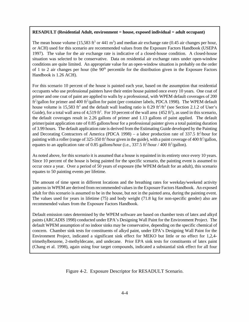
RESADULT (Residential Adult, environment = house, exposed individual = adult occupant)
The mean house volume (15,583 ft3 or 441 m3) and median air exchange rate (0.45 air changes per hour,or ACH) used for this scenario are recommended values from the Exposure Factors Handbook (USEPA1997). The value for the air exchange rate is indicative of a closed-house condition. A closed-housesituation was selected to be conservative. Data on residential air exchange rates under open-windowconditions are quite limited. An appropriate value for an open-window situation is probably on the orderof 1 to 2 air changes per hour (the 90th percentile for the distribution given in the Exposure FactorsHandbook is 1.26 ACH).
For this scenario 10 percent of the house is painted each year, based on the assumption that residentialoccupants who use professional painters have their entire house painted once every 10 years. One coat ofprimer and one coat of paint are applied to walls by a professional, with WPEM default coverages of 200ft2/gallon for primer and 400 ft2/gallon for paint (per container labels, PDCA 1998). The WPEM defaulthouse volume is 15,583 ft3 and the default wall loading ratio is 0.29 ft2/ft3 (see Section 2.1.2 of User’sGuide), for a total wall area of 4,519 ft2. For 10 percent of the wall area (452 ft2), as used in this scenario,the default coverages result in 2.26 gallons of primer and 1.13 gallons of paint applied. The defaultprimer/paint application rate of 0.85 gallons/hour for a professional painter gives a total painting durationof 3.99 hours. The default application rate is derived from the Estimating Guide developed by the Paintingand Decorating Contractors of America (PDCA 1998) – a labor production rate of 337.5 ft2/hour forpainting with a roller (range of 325-350 ft2/hour given in the guide), with a paint coverage of 400 ft2/gallon,equates to an application rate of 0.85 gallons/hour (i.e., 337.5 ft2/hour / 400 ft2/gallon).
As noted above, for this scenario it is assumed that a house is repainted in its entirety once every 10 years.Since 10 percent of the house is being painted for the specific scenario, the painting event is assumed tooccur once a year. Over a period of 50 years of exposure (the WPEM default for an adult), this scenarioequates to 50 painting events per lifetime.
The amount of time spent in different locations and the breathing rates for weekday/weekend activitypatterns in WPEM are derived from recommended values in the Exposure Factors Handbook. An exposedadult for this scenario is assumed to be in the house, but not in the painted area, during the painting event.The values used for years in lifetime (75) and body weight (71.8 kg for non-specific gender) also arerecommended values from the Exposure Factors Handbook.
Default emission rates determined by the WPEM software are based on chamber tests of latex and alkydpaints (ARCADIS 1998) conducted under EPA’s Designing Wall Paint for the Environment Project. Thedefault WPEM assumption of no indoor sinks may be conservative, depending on the specific chemical ofconcern. Chamber sink tests for constituents of alkyd paint, under EPA’s Designing Wall Paint for theEnvironment Project, indicated a significant sink effect for MEKO but little or no effect for 1,2,4-trimethylbenzene, 2-methyldecane, and undecane. Prior EPA sink tests for constituents of latex paint(Chang et al. 1998), again using four target compounds, indicated a substantial sink effect for all four
Figure 4-2. Exposure Descriptor for RESADULT Scenario.
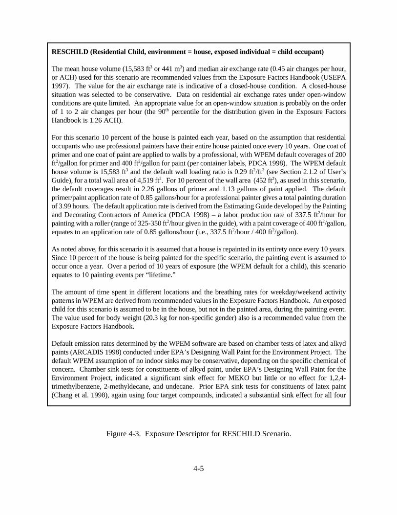
4-5
RESCHILD (Residential Child, environment = house, exposed individual = child occupant)
The mean house volume (15,583 ft3 or 441 m3) and median air exchange rate (0.45 air changes per hour,or ACH) used for this scenario are recommended values from the Exposure Factors Handbook (USEPA1997). The value for the air exchange rate is indicative of a closed-house condition. A closed-housesituation was selected to be conservative. Data on residential air exchange rates under open-windowconditions are quite limited. An appropriate value for an open-window situation is probably on the orderof 1 to 2 air changes per hour (the 90th percentile for the distribution given in the Exposure FactorsHandbook is 1.26 ACH).
For this scenario 10 percent of the house is painted each year, based on the assumption that residentialoccupants who use professional painters have their entire house painted once every 10 years. One coat ofprimer and one coat of paint are applied to walls by a professional, with WPEM default coverages of 200ft2/gallon for primer and 400 ft2/gallon for paint (per container labels, PDCA 1998). The WPEM defaulthouse volume is 15,583 ft3 and the default wall loading ratio is 0.29 ft2/ft3 (see Section 2.1.2 of User’sGuide), for a total wall area of 4,519 ft2. For 10 percent of the wall area (452 ft2), as used in this scenario,the default coverages result in 2.26 gallons of primer and 1.13 gallons of paint applied. The defaultprimer/paint application rate of 0.85 gallons/hour for a professional painter gives a total painting durationof 3.99 hours. The default application rate is derived from the Estimating Guide developed by the Paintingand Decorating Contractors of America (PDCA 1998) – a labor production rate of 337.5 ft2/hour forpainting with a roller (range of 325-350 ft2/hour given in the guide), with a paint coverage of 400 ft2/gallon,equates to an application rate of 0.85 gallons/hour (i.e., 337.5 ft2/hour / 400 ft2/gallon).
As noted above, for this scenario it is assumed that a house is repainted in its entirety once every 10 years.Since 10 percent of the house is being painted for the specific scenario, the painting event is assumed tooccur once a year. Over a period of 10 years of exposure (the WPEM default for a child), this scenarioequates to 10 painting events per “lifetime.”
The amount of time spent in different locations and the breathing rates for weekday/weekend activitypatterns in WPEM are derived from recommended values in the Exposure Factors Handbook. An exposedchild for this scenario is assumed to be in the house, but not in the painted area, during the painting event.The value used for body weight (20.3 kg for non-specific gender) also is a recommended value from theExposure Factors Handbook.
Default emission rates determined by the WPEM software are based on chamber tests of latex and alkydpaints (ARCADIS 1998) conducted under EPA’s Designing Wall Paint for the Environment Project. Thedefault WPEM assumption of no indoor sinks may be conservative, depending on the specific chemical ofconcern. Chamber sink tests for constituents of alkyd paint, under EPA’s Designing Wall Paint for theEnvironment Project, indicated a significant sink effect for MEKO but little or no effect for 1,2,4-trimethylbenzene, 2-methyldecane, and undecane. Prior EPA sink tests for constituents of latex paint(Chang et al. 1998), again using four target compounds, indicated a substantial sink effect for all four
Figure 4-3. Exposure Descriptor for RESCHILD Scenario.
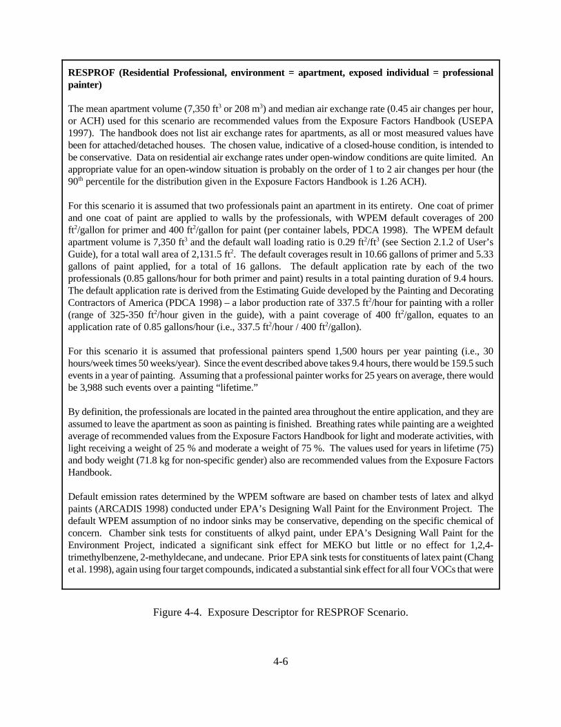
4-6
RESPROF (Residential Professional, environment = apartment, exposed individual = professionalpainter)
The mean apartment volume (7,350 ft3 or 208 m3) and median air exchange rate (0.45 air changes per hour,or ACH) used for this scenario are recommended values from the Exposure Factors Handbook (USEPA1997). The handbook does not list air exchange rates for apartments, as all or most measured values havebeen for attached/detached houses. The chosen value, indicative of a closed-house condition, is intended tobe conservative. Data on residential air exchange rates under open-window conditions are quite limited. Anappropriate value for an open-window situation is probably on the order of 1 to 2 air changes per hour (the90th percentile for the distribution given in the Exposure Factors Handbook is 1.26 ACH).
For this scenario it is assumed that two professionals paint an apartment in its entirety. One coat of primerand one coat of paint are applied to walls by the professionals, with WPEM default coverages of 200ft2/gallon for primer and 400 ft2/gallon for paint (per container labels, PDCA 1998). The WPEM defaultapartment volume is 7,350 ft3 and the default wall loading ratio is 0.29 ft2/ft3 (see Section 2.1.2 of User’sGuide), for a total wall area of 2,131.5 ft2. The default coverages result in 10.66 gallons of primer and 5.33gallons of paint applied, for a total of 16 gallons. The default application rate by each of the twoprofessionals (0.85 gallons/hour for both primer and paint) results in a total painting duration of 9.4 hours.The default application rate is derived from the Estimating Guide developed by the Painting and DecoratingContractors of America (PDCA 1998) – a labor production rate of 337.5 ft2/hour for painting with a roller(range of 325-350 ft2/hour given in the guide), with a paint coverage of 400 ft2/gallon, equates to anapplication rate of 0.85 gallons/hour (i.e., 337.5 ft2/hour / 400 ft2/gallon).
For this scenario it is assumed that professional painters spend 1,500 hours per year painting (i.e., 30hours/week times 50 weeks/year). Since the event described above takes 9.4 hours, there would be 159.5 suchevents in a year of painting. Assuming that a professional painter works for 25 years on average, there wouldbe 3,988 such events over a painting “lifetime.”
By definition, the professionals are located in the painted area throughout the entire application, and they areassumed to leave the apartment as soon as painting is finished. Breathing rates while painting are a weightedaverage of recommended values from the Exposure Factors Handbook for light and moderate activities, withlight receiving a weight of 25 % and moderate a weight of 75 %. The values used for years in lifetime (75)and body weight (71.8 kg for non-specific gender) also are recommended values from the Exposure FactorsHandbook.
Default emission rates determined by the WPEM software are based on chamber tests of latex and alkydpaints (ARCADIS 1998) conducted under EPA’s Designing Wall Paint for the Environment Project. Thedefault WPEM assumption of no indoor sinks may be conservative, depending on the specific chemical ofconcern. Chamber sink tests for constituents of alkyd paint, under EPA’s Designing Wall Paint for theEnvironment Project, indicated a significant sink effect for MEKO but little or no effect for 1,2,4-trimethylbenzene, 2-methyldecane, and undecane. Prior EPA sink tests for constituents of latex paint (Changet al. 1998), again using four target compounds, indicated a substantial sink effect for all four VOCs that were
Figure 4-4. Exposure Descriptor for RESPROF Scenario.
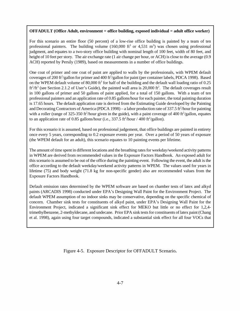
4-7
OFFADULT (Office Adult, environment = office building, exposed individual = adult office worker)
For this scenario an entire floor (50 percent) of a low-rise office building is painted by a team of tenprofessional painters. The building volume (160,000 ft3 or 4,531 m3) was chosen using professionaljudgment, and equates to a two-story office building with nominal length of 100 feet, width of 80 feet, andheight of 10 feet per story. The air exchange rate (1 air change per hour, or ACH) is close to the average (0.9ACH) reported by Persily (1989), based on measurements in a number of office buildings.
One coat of primer and one coat of paint are applied to walls by the professionals, with WPEM defaultcoverages of 200 ft2/gallon for primer and 400 ft2/gallon for paint (per container labels, PDCA 1998). Basedon the WPEM default volume of 80,000 ft3 for half of the building and the default wall loading ratio of 0.25ft2/ft3 (see Section 2.1.2 of User’s Guide), the painted wall area is 20,000 ft2. The default coverages resultin 100 gallons of primer and 50 gallons of paint applied, for a total of 150 gallons. With a team of tenprofessional painters and an application rate of 0.85 gallons/hour for each painter, the total painting durationis 17.65 hours. The default application rate is derived from the Estimating Guide developed by the Paintingand Decorating Contractors of America (PDCA 1998) – a labor production rate of 337.5 ft2/hour for paintingwith a roller (range of 325-350 ft2/hour given in the guide), with a paint coverage of 400 ft2/gallon, equatesto an application rate of 0.85 gallons/hour (i.e., 337.5 ft2/hour / 400 ft2/gallon).
For this scenario it is assumed, based on professional judgement, that office buildings are painted in entiretyonce every 5 years, corresponding to 0.2 exposure events per year. Over a period of 50 years of exposure(the WPEM default for an adult), this scenario equates to 10 painting events per lifetime.
The amount of time spent in different locations and the breathing rates for weekday/weekend activity patternsin WPEM are derived from recommended values in the Exposure Factors Handbook. An exposed adult forthis scenario is assumed to be out of the office during the painting event. Following the event, the adult is theoffice according to the default weekday/weekend activity patterns in WPEM. The values used for years inlifetime (75) and body weight (71.8 kg for non-specific gender) also are recommended values from theExposure Factors Handbook.
Default emission rates determined by the WPEM software are based on chamber tests of latex and alkydpaints (ARCADIS 1998) conducted under EPA’s Designing Wall Paint for the Environment Project. Thedefault WPEM assumption of no indoor sinks may be conservative, depending on the specific chemical ofconcern. Chamber sink tests for constituents of alkyd paint, under EPA’s Designing Wall Paint for theEnvironment Project, indicated a significant sink effect for MEKO but little or no effect for 1,2,4-trimethylbenzene, 2-methyldecane, and undecane. Prior EPA sink tests for constituents of latex paint (Changet al. 1998), again using four target compounds, indicated a substantial sink effect for all four VOCs that
Figure 4-5. Exposure Descriptor for OFFADULT Scenario.
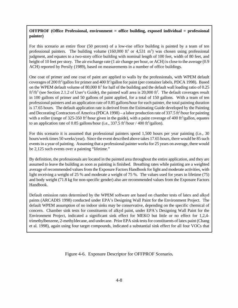
4-8
OFFPROF (Office Professional, environment = office building, exposed individual = professionalpainter)
For this scenario an entire floor (50 percent) of a low-rise office building is painted by a team of tenprofessional painters. The building volume (160,000 ft3 or 4,531 m3) was chosen using professionaljudgment, and equates to a two-story office building with nominal length of 100 feet, width of 80 feet, andheight of 10 feet per story. The air exchange rate (1 air change per hour, or ACH) is close to the average (0.9ACH) reported by Persily (1989), based on measurements in a number of office buildings.
One coat of primer and one coat of paint are applied to walls by the professionals, with WPEM defaultcoverages of 200 ft2/gallon for primer and 400 ft2/gallon for paint (per container labels, PDCA 1998). Basedon the WPEM default volume of 80,000 ft3 for half of the building and the default wall loading ratio of 0.25ft2/ft3 (see Section 2.1.2 of User’s Guide), the painted wall area is 20,000 ft2. The default coverages resultin 100 gallons of primer and 50 gallons of paint applied, for a total of 150 gallons. With a team of tenprofessional painters and an application rate of 0.85 gallons/hour for each painter, the total painting durationis 17.65 hours. The default application rate is derived from the Estimating Guide developed by the Paintingand Decorating Contractors of America (PDCA 1998) – a labor production rate of 337.5 ft2/hour for paintingwith a roller (range of 325-350 ft2/hour given in the guide), with a paint coverage of 400 ft2/gallon, equatesto an application rate of 0.85 gallons/hour (i.e., 337.5 ft2/hour / 400 ft2/gallon).
For this scenario it is assumed that professional painters spend 1,500 hours per year painting (i.e., 30hours/week times 50 weeks/year). Since the event described above takes 17.65 hours, there would be 85 suchevents in a year of painting. Assuming that a professional painter works for 25 years on average, there wouldbe 2,125 such events over a painting “lifetime.”
By definition, the professionals are located in the painted area throughout the entire application, and they areassumed to leave the building as soon as painting is finished. Breathing rates while painting are a weightedaverage of recommended values from the Exposure Factors Handbook for light and moderate activities, withlight receiving a weight of 25 % and moderate a weight of 75 %. The values used for years in lifetime (75)and body weight (71.8 kg for non-specific gender) also are recommended values from the Exposure FactorsHandbook.
Default emission rates determined by the WPEM software are based on chamber tests of latex and alkydpaints (ARCADIS 1998) conducted under EPA’s Designing Wall Paint for the Environment Project. Thedefault WPEM assumption of no indoor sinks may be conservative, depending on the specific chemical ofconcern. Chamber sink tests for constituents of alkyd paint, under EPA’s Designing Wall Paint for theEnvironment Project, indicated a significant sink effect for MEKO but little or no effect for 1,2,4-trimethylbenzene, 2-methyldecane, and undecane. Prior EPA sink tests for constituents of latex paint (Changet al. 1998), again using four target compounds, indicated a substantial sink effect for all four VOCs that
Figure 4-6. Exposure Descriptor for OFFPROF Scenario.
4-9
4.3 Some Application Tips
Once inputs have been supplied and saved as needed, and the model has been executed, theuser may wish to model some other scenario that is different from the one just modeled. To resetall model input parameters to their initial default values, it is not necessary to close WPEM and thenreopen the software. The same effect can be achieved by clicking on File at the top left of thescreen, then New. Alternatively, a file for a default scenario can be selected to insert the defaultvalues for that scenario.
If the user selects a file for one of the default scenarios and then edits the file, it is advisableto save the edits under a new file name, rather than overwriting the file that contains the defaultscenario. The user is further advised to make copies of the default scenario files (the six sets of filesprovided with the model that have extensions of .wem and .we1) in a directory that is different fromthe one from which WPEM is executed (by default, the install package for WPEM places all files inc:\program files\wpem). With this safeguard, a default-scenario file can be restored to its originalvalues in the event that it is inadvertently overwritten, without the need to re-install the software.
The user also may wish to have a customized list of default values for his/her own use. Thesimplest way of accomplishing this is to first reset all values to their initial defaults (as occurs whenfirst opening WPEM or when clicking on File, then New). Next, the appropriate inputs can beedited to the values that the user would like to keep as a basic set of defaults. Once all edits havebeen completed, they can be saved to a file with a name of the user’s choice by clicking on File,then Save As.
The WPEM software is sufficiently flexible to model a wide variety of situations. Forexample, even a chamber test can be simulated using the software. The volume of the chamber canbe input by selecting residence, for example, and then editing the building volume. The user alsoshould make the choice that the entire building is painted, so that WPEM will use calculations for asingle-zone model. Next, the air exchange rate should be edited to match the conditions for thechamber test. The value for the interzonal airflow rate does not matter because a single-zone modelwill be used. Then one of the painted-surface choices (e.g., walls only) can be selected and thevalue edited to match the loading in the chamber. The coverage or film thickness also should beedited to match the modeled application. For small-chamber tests, the paint usually is appliednearly instantaneously outside the chamber, after which the painted specimen is inserted. To matchthis condition closely, the number of painters or the application rate can be edited so that thecalculated priming or painting duration (whichever applies) is a small value such as 0.01 hours. Theremaining edits would pertain to the type of paint and chemical to be modeled.
5-1
5. REFERENCES
ARCADIS, 1998. Testing to Determine Chemical Emissions from Paint in Support of the EPADesigning Wall Paint for the Indoor Environment Project – Description of the Testing Programand Results. Final report prepared by ARCADIS Geraghty & Miller, Inc., for USEPA Office ofPollution Prevention and Toxics under EPA Contract No. 68-W6-0023.
Chang, JCS, Sparks, LE, Guo, Z, and Fortmann, R, 1998. “Evaluation of Sinks Effects on VOCsfrom a Latex Paint,” J. Air & Waste Manage. Assoc. 48:953-958.
Evans, WC, 1994. “Development of Continuous-Application Source Terms and AnalyticalSolutions for One- and Two-Compartment Systems.” In Characterizing Sources of Indoor AirPollution and Related Sink Effects, ASTM STP 1287, American Society for Testing andMaterials, pp 279-293.
Koontz, MD, and Rector, HR, 1995. Estimation of Distributions for Residential Air ExchangeRates. Final report prepared by GEOMET Technologies, Inc., for USEPA Office of PollutionPrevention and Toxics.
PDCA, 1998. Estimating Guide, Nineteenth Edition. Published by the Painting and DecoratingContractors of America, Fairfax, VA.
Matthews, JH, 1992. Numerical Methods for Mathematics, Science, and Engineering, SecondEdition, Prentice Hall, Englewood Cliffs, NJ.
Persily, AK, 1989. “Ventilation Rates in Office Buildings,” In IAQ 1989, American Society ofHeating, Refrigerating and Air-Conditioning Engineers (ASHRAE), pp 128-136.
USEPA, 1992. Guidelines for Exposure Assessment. EPA/600/Z-92/001, U.S. EnvironmentalProtection Agency, Office of Research and Development, Office of Health and EnvironmentalAssessment.
USEPA, 1997. Exposure Factors Handbook, Volumes I-III. EPA/600/P-95/002Fa, b, c, U.S.Environmental Protection Agency, Office of Research and Development, National Center forEnvironmental Assessment.
WESTAT, 1987. Household Solvent Products: A National Usage Survey. Final report preparedfor USEPA Office of Pollution Prevention and Toxics under EPA Contract No. 68-02-4243.

APPENDIX A
ALKYD PAINT CHAMBER TESTS
A-1
A1. INTRODUCTION
A series of small-chamber tests was conducted by ARCADIS Geraghty and Miller, Inc., to
(1) characterize concentrations of various volatile organic compounds (VOCs) emitted from
different formulations of alkyd primer and paint, and (2) to explore the interactions of some of
these compounds with selected indoor sinks. In addition to the broad objectives of improving the
understanding of emission and sink behavior for these chemicals in alkyd primer and paint, a more
specific objective was to provide a quantitative basis for development of emission/sink models or
for estimating parameters for such models. In addition to the small-chamber tests, ARCADIS
Geraghty and Miller, Inc., conducted painting events at EPA’s research house in North Carolina
for the primary purpose of gathering data to be used for model evaluation.
The sections that follow describe methods and results for bulk analysis of the alkyd
primer/paint formulations prior to chamber testing, small-chamber emission tests of these
formulations, development of predictive models for VOC emissions from alkyd primer and paint,
and sink behavior of selected chemicals in alkyd primer or paint.
A2. BULK ANALYSIS
Prior to conduct of small-chamber emission tests, each formulation of alkyd primer or
paint was analyzed to determine its chemical composition by weight. In brief, the procedure for
analysis of the bulk product that was followed by ARCADIS Geraghty and Miller, Inc.,
(ARCADIS 1998) involved (1) extracting alkyd primer and paints with methylene chloride, (2)
centrifuging the sample to remove solids, and (3) analyzing the supernatant by GC/MS.
Results of the bulk analysis are shown as chemical weight fractions (mg/g) in Table A-1.
The primary constituents of both the primer (formulation AP-F) and one of the paints
(formulation ASG-G) were propyl-cyclohexane, decane, and undecane. The second paint
(formulation ASG-H) was dominated by 2-methyldecane and various branched undecanes.
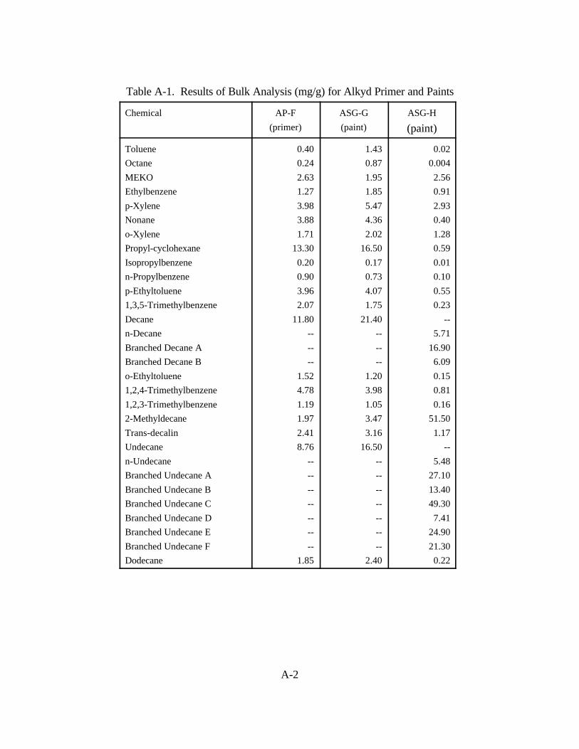
A-2
Table A-1. Results of Bulk Analysis (mg/g) for Alkyd Primer and Paints
Chemical AP-F
(primer)
ASG-G
(paint)
ASG-H
(paint)
Toluene
Octane
MEKO
Ethylbenzene
p-Xylene
Nonane
o-Xylene
Propyl-cyclohexane
Isopropylbenzene
n-Propylbenzene
p-Ethyltoluene
1,3,5-Trimethylbenzene
Decane
n-Decane
Branched Decane A
Branched Decane B
o-Ethyltoluene
1,2,4-Trimethylbenzene
1,2,3-Trimethylbenzene
2-Methyldecane
Trans-decalin
Undecane
n-Undecane
Branched Undecane A
Branched Undecane B
Branched Undecane C
Branched Undecane D
Branched Undecane E
Branched Undecane F
Dodecane
0.40
0.24
2.63
1.27
3.98
3.88
1.71
13.30
0.20
0.90
3.96
2.07
11.80
--
--
--
1.52
4.78
1.19
1.97
2.41
8.76
--
--
--
--
--
--
--
1.85
1.43
0.87
1.95
1.85
5.47
4.36
2.02
16.50
0.17
0.73
4.07
1.75
21.40
--
--
--
1.20
3.98
1.05
3.47
3.16
16.50
--
--
--
--
--
--
--
2.40
0.02
0.004
2.56
0.91
2.93
0.40
1.28
0.59
0.01
0.10
0.55
0.23
--
5.71
16.90
6.09
0.15
0.81
0.16
51.50
1.17
--
5.48
27.10
13.40
49.30
7.41
24.90
21.30
0.22

A-3
A3. SMALL-CHAMBER EMISSION TESTS
The small-chamber emission tests were conducted by ARCADIS Geraghty and Miller,
Inc., in the EPA APPCD Source Characterization Laboratories located in the EPA Environmental
Research Center in Research Triangle Park, NC. The tests were conducted using 53-liter,
stainless-steel chambers housed in a temperature-controlled incubator. These chambers have been
fitted with inlet and outlet manifolds for the air supply, temperature and relative humidity sensors,
and a small fan to ensure mixing within the chamber. During each test, clean (VOC- and particle-
free) air was supplied to the chamber at a controlled relative humidity. A glass sampling manifold
has been connected to the chamber outlet for collection of air samples.
The substrate used in the tests was 0.5-inch gypsum wallboard that was purchased from a
local retail outlet in North Carolina. For each test, the substrate was cut to a size of 16 by 16 cm
(total area of 256 cm2 or 0.0256 m2), resulting in a surface-to-volume loading ratio of about 0.5
m2/m3 in the chamber. The edges were sealed and the test specimen was placed on the floor of
the chamber during the test. The cut and sealed substrate was conditioned in the chamber for at
least 24 hours prior to application of primer/paint.
Primer and paint were applied to the wallboard with a roller purchased at a local retail
outlet. The rate of primer/paint application in the tests, and resulting wet film thickness, were
based on recommendations from the manufacturers. The mass of paint applied was determined
gravimetrically by two methods. Wet film thickness was not measured with a gage during the
tests because the gage affects surface film characteristics and the specimen was to be inserted into
the chamber as quickly as possible after priming or painting. Based on the measured mass of paint
applied and the known specific gravity of the coating, the average calculated wet film thickness
was 415 Fm (16.4 mil) for the alkyd primer and 105 Fm (4.1 mil) for the alkyd paint.
As noted above, the wallboard specimen was conditioned in the chamber at least 24 hours
before the test. Background concentrations were measured prior to removing the specimen.
Primer then was applied, the specimen was re-inserted in the chamber, and air samples were
collected for the next 48 hours. Then the specimen was removed, paint was applied, the
wallboard again was inserted in the chamber, and air samples were collected during the next 12
days. Thus, the total monitoring period for each test was 14 days in duration.
Two tests were conducted for alkyd primer and paint. The primer AP-F, for which the
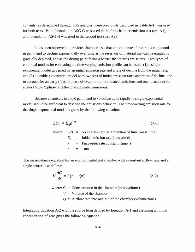
A-4
contents (as determined through bulk analysis) were previously described in Table A-1, was used
for both tests. Paint formulation ASG-G was used in the first chamber emission test (test A1),
and formulation ASG-H was used in the second test (test A2).
It has been observed in previous chamber tests that emission rates for various compounds
in paint tend to decline exponentially over time as the reservoir of material that can be emitted is
gradually depleted, and as the drying paint forms a barrier that retards emissions. Two types of
empirical models for estimating the time-varying emission profile can be used: (1) a single-
exponential model governed by an initial emission rate and a rate of decline from the initial rate,
and (2) a double-exponential model with two sets of initial emission rates and rates of decline, one
to account for an early (“fast”) phase of evaporation-dominated emissions and one to account for
a later (“slow”) phase of diffusion-dominated emissions.
Because chemicals in alkyd paint tend to volatilize quite rapidly, a single-exponential
model should be sufficient to describe the emissions behavior. The time-varying emission rate for
the single-exponential model is given by the following equation:
(A-1)S t E e kt( ) = −0
where: S(t) = Source strength as a function of time (mass/time)
E0 = Initial emission rate (mass/time)
k = First-order rate constant (time-1)
t = Time.
The mass-balance equation for an environmental test chamber with a constant airflow rate and a
single source is as follows:
(A-2)VdC
dtS t QC= −( )
where: C = Concentration in the chamber (mass/volume)
V = Volume of the chamber
Q = Airflow rate into and out of the chamber (volume/time).
Integrating Equation A-2 with the source term defined by Equation A-1 and assuming an initial
concentration of zero gives the following equation:
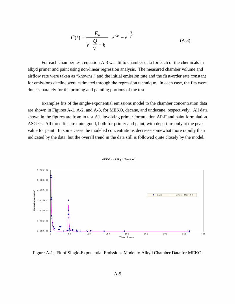
A-5
M E K O - - A l k y d T e s t A 1
0 . 0 0 E + 0 0
1 . 0 0 E + 0 1
2 . 0 0 E + 0 1
3 . 0 0 E + 0 1
4 . 0 0 E + 0 1
5 . 0 0 E + 0 1
6 . 0 0 E + 0 1
0 5 0 1 0 0 1 5 0 2 0 0 2 5 0 3 0 0 3 5 0 4 0 0
T i m e , h o u r s
Co
nce
ntr
atio
n, m
g/m
3
D a t a L i n e o f B e s t F i t
(A-3)C t
E
VQ
Vk
e ektQ
Vt
( ) =−
−
− −0
For each chamber test, equation A-3 was fit to chamber data for each of the chemicals in
alkyd primer and paint using non-linear regression analysis. The measured chamber volume and
airflow rate were taken as “knowns,” and the initial emission rate and the first-order rate constant
for emissions decline were estimated through the regression technique. In each case, the fits were
done separately for the priming and painting portions of the test.
Examples fits of the single-exponential emissions model to the chamber concentration data
are shown in Figures A-1, A-2, and A-3, for MEKO, decane, and undecane, respectively. All data
shown in the figures are from in test A1, involving primer formulation AP-F and paint formulation
ASG-G. All three fits are quite good, both for primer and paint, with departure only at the peak
value for paint. In some cases the modeled concentrations decrease somewhat more rapidly than
indicated by the data, but the overall trend in the data still is followed quite closely by the model.
Figure A-1. Fit of Single-Exponential Emissions Model to Alkyd Chamber Data for MEKO.
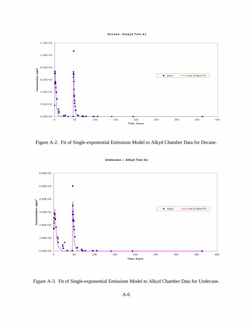
A-6
D e c a n e - - A l y k y d T e s t A 1
0 .00E+00
2 .00E+02
4 .00E+02
6 .00E+02
8 .00E+02
1 .00E+03
1 .20E+03
0 5 0 100 150 200 250 300 350 400
Time, hours
Co
nce
ntr
atio
n, m
g/m
3
Data Line of Best F i t
Undecane -- Alkyd Test A1
0.00E+00
1.00E+02
2.00E+02
3.00E+02
4.00E+02
5.00E+02
6.00E+02
0 50 100 150 200 250 300 350 400
Time, hours
Co
nce
ntr
atio
n, m
g/m
3
Data Line of Best Fit
Figure A-2. Fit of Single-exponential Emissions Model to Alkyd Chamber Data for Decane.
Figure A-3. Fit of Single-exponential Emissions Model to Alkyd Chamber Data for Undecane.
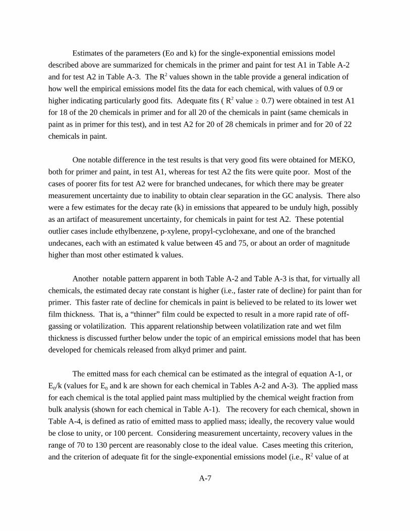
A-7
Estimates of the parameters (Eo and k) for the single-exponential emissions model
described above are summarized for chemicals in the primer and paint for test A1 in Table A-2
and for test A2 in Table A-3. The R2 values shown in the table provide a general indication of
how well the empirical emissions model fits the data for each chemical, with values of 0.9 or
higher indicating particularly good fits. Adequate fits ( R2 value $ 0.7) were obtained in test A1
for 18 of the 20 chemicals in primer and for all 20 of the chemicals in paint (same chemicals in
paint as in primer for this test), and in test A2 for 20 of 28 chemicals in primer and for 20 of 22
chemicals in paint.
One notable difference in the test results is that very good fits were obtained for MEKO,
both for primer and paint, in test A1, whereas for test A2 the fits were quite poor. Most of the
cases of poorer fits for test A2 were for branched undecanes, for which there may be greater
measurement uncertainty due to inability to obtain clear separation in the GC analysis. There also
were a few estimates for the decay rate (k) in emissions that appeared to be unduly high, possibly
as an artifact of measurement uncertainty, for chemicals in paint for test A2. These potential
outlier cases include ethylbenzene, p-xylene, propyl-cyclohexane, and one of the branched
undecanes, each with an estimated k value between 45 and 75, or about an order of magnitude
higher than most other estimated k values.
Another notable pattern apparent in both Table A-2 and Table A-3 is that, for virtually all
chemicals, the estimated decay rate constant is higher (i.e., faster rate of decline) for paint than for
primer. This faster rate of decline for chemicals in paint is believed to be related to its lower wet
film thickness. That is, a “thinner” film could be expected to result in a more rapid rate of off-
gassing or volatilization. This apparent relationship between volatilization rate and wet film
thickness is discussed further below under the topic of an empirical emissions model that has been
developed for chemicals released from alkyd primer and paint.
The emitted mass for each chemical can be estimated as the integral of equation A-1, or
E0/k (values for E0 and k are shown for each chemical in Tables A-2 and A-3). The applied mass
for each chemical is the total applied paint mass multiplied by the chemical weight fraction from
bulk analysis (shown for each chemical in Table A-1). The recovery for each chemical, shown in
Table A-4, is defined as ratio of emitted mass to applied mass; ideally, the recovery value would
be close to unity, or 100 percent. Considering measurement uncertainty, recovery values in the
range of 70 to 130 percent are reasonably close to the ideal value. Cases meeting this criterion,
and the criterion of adequate fit for the single-exponential emissions model (i.e., R2 value of at
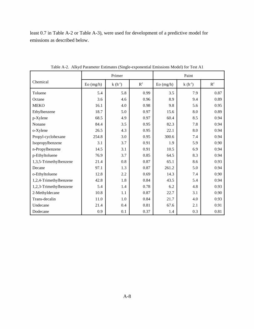
A-8
least 0.7 in Table A-2 or Table A-3), were used for development of a predictive model for
emissions as described below.
Table A-2. Alkyd Parameter Estimates (Single-exponential Emissions Model) for Test A1
Chemical
Primer Paint
Eo (mg/h) k (h-1) R2 Eo (mg/h) k (h-1) R2
Toluene
Octane
MEKO
Ethylbenzene
p-Xylene
Nonane
o-Xylene
Propyl-cyclohexane
Isopropylbenzene
n-Propylbenzene
p-Ethyltoluene
1,3,5-Trimethylbenzene
Decane
o-Ethyltoluene
1,2,4-Trimethylbenzene
1,2,3-Trimethylbenzene
2-Methyldecane
Trans-decalin
Undecane
Dodecane
5.4
3.6
16.1
18.7
68.5
84.4
26.5
254.8
3.1
14.5
76.9
21.4
97.1
12.8
42.8
5.4
10.8
11.0
21.4
0.9
5.8
4.6
4.0
5.0
4.9
3.5
4.3
3.0
3.7
3.1
3.7
0.8
1.3
2.2
1.8
1.4
1.1
1.0
0.4
0.1
0.99
0.96
0.98
0.97
0.97
0.95
0.95
0.95
0.91
0.91
0.85
0.87
0.87
0.69
0.84
0.78
0.87
0.84
0.81
0.37
3.5
8.9
9.8
15.6
60.4
82.3
22.1
300.6
1.9
10.5
64.5
65.1
261.2
14.3
43.5
6.2
22.7
21.7
67.6
1.4
7.9
9.4
5.6
8.0
8.5
7.8
8.0
7.4
5.9
6.9
8.3
8.6
5.0
7.4
5.4
4.8
3.1
4.0
2.1
0.3
0.87
0.89
0.95
0.89
0.94
0.94
0.94
0.94
0.90
0.94
0.94
0.93
0.94
0.90
0.94
0.93
0.90
0.93
0.91
0.81
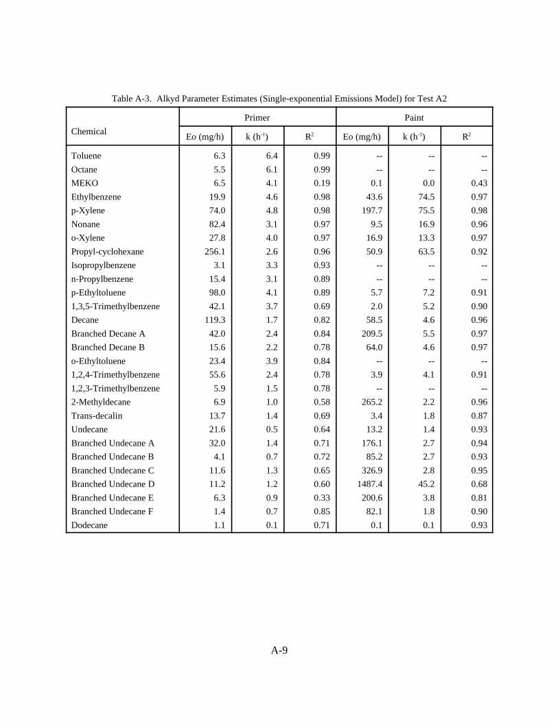
A-9
Table A-3. Alkyd Parameter Estimates (Single-exponential Emissions Model) for Test A2
Chemical
Primer Paint
Eo (mg/h) k (h-1) R2 Eo (mg/h) k (h-1) R2
Toluene
Octane
MEKO
Ethylbenzene
p-Xylene
Nonane
o-Xylene
Propyl-cyclohexane
Isopropylbenzene
n-Propylbenzene
p-Ethyltoluene
1,3,5-Trimethylbenzene
Decane
Branched Decane A
Branched Decane B
o-Ethyltoluene
1,2,4-Trimethylbenzene
1,2,3-Trimethylbenzene
2-Methyldecane
Trans-decalin
Undecane
Branched Undecane A
Branched Undecane B
Branched Undecane C
Branched Undecane D
Branched Undecane E
Branched Undecane F
Dodecane
6.3
5.5
6.5
19.9
74.0
82.4
27.8
256.1
3.1
15.4
98.0
42.1
119.3
42.0
15.6
23.4
55.6
5.9
6.9
13.7
21.6
32.0
4.1
11.6
11.2
6.3
1.4
1.1
6.4
6.1
4.1
4.6
4.8
3.1
4.0
2.6
3.3
3.1
4.1
3.7
1.7
2.4
2.2
3.9
2.4
1.5
1.0
1.4
0.5
1.4
0.7
1.3
1.2
0.9
0.7
0.1
0.99
0.99
0.19
0.98
0.98
0.97
0.97
0.96
0.93
0.89
0.89
0.69
0.82
0.84
0.78
0.84
0.78
0.78
0.58
0.69
0.64
0.71
0.72
0.65
0.60
0.33
0.85
0.71
--
--
0.1
43.6
197.7
9.5
16.9
50.9
--
--
5.7
2.0
58.5
209.5
64.0
--
3.9
--
265.2
3.4
13.2
176.1
85.2
326.9
1487.4
200.6
82.1
0.1
--
--
0.0
74.5
75.5
16.9
13.3
63.5
--
--
7.2
5.2
4.6
5.5
4.6
--
4.1
--
2.2
1.8
1.4
2.7
2.7
2.8
45.2
3.8
1.8
0.1
--
--
0.43
0.97
0.98
0.96
0.97
0.92
--
--
0.91
0.90
0.96
0.97
0.97
--
0.91
--
0.96
0.87
0.93
0.94
0.93
0.95
0.68
0.81
0.90
0.93
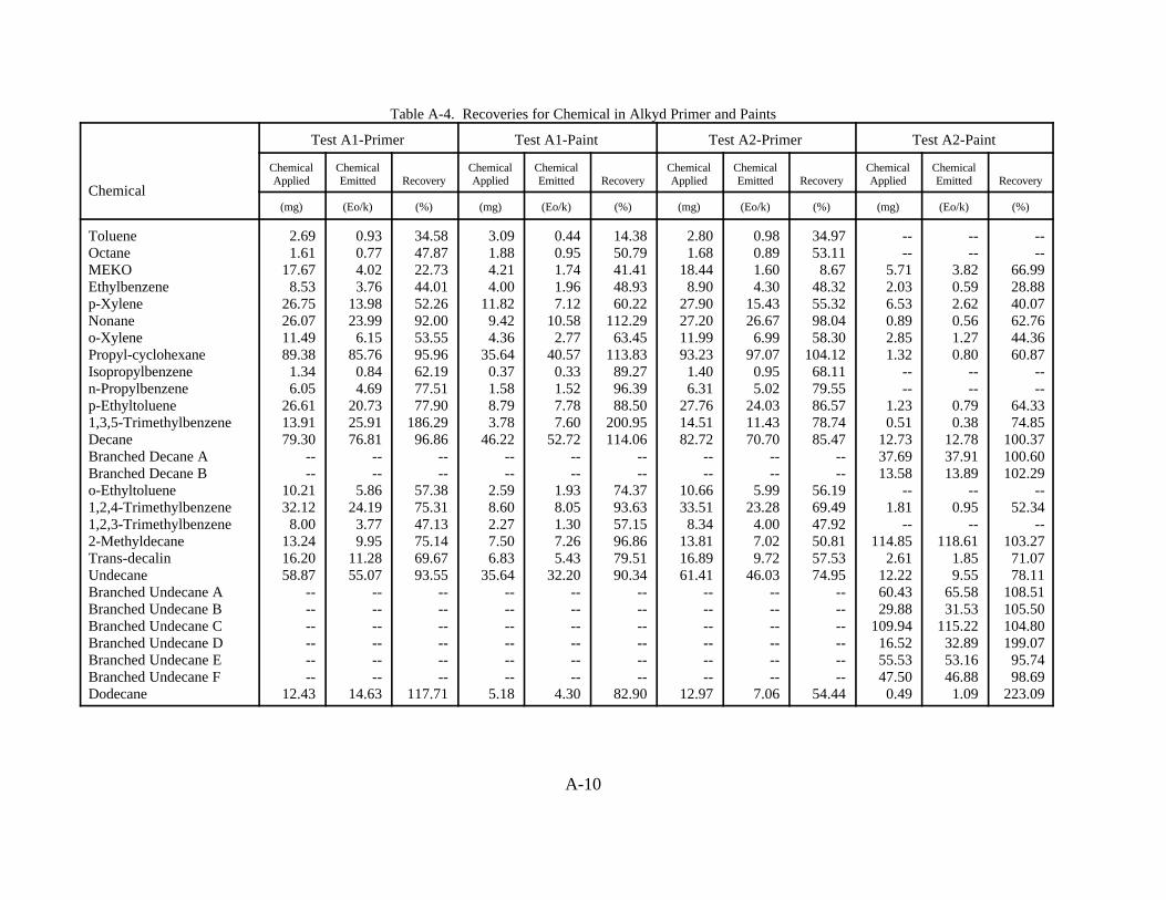
A-10
Table A-4. Recoveries for Chemical in Alkyd Primer and Paints
Chemical
Test A1-Primer Test A1-Paint Test A2-Primer Test A2-Paint
ChemicalApplied
ChemicalEmitted Recovery
ChemicalApplied
ChemicalEmitted Recovery
ChemicalApplied
ChemicalEmitted Recovery
ChemicalApplied
ChemicalEmitted Recovery
(mg) (Eo/k) (%) (mg) (Eo/k) (%) (mg) (Eo/k) (%) (mg) (Eo/k) (%)
TolueneOctaneMEKOEthylbenzenep-XyleneNonaneo-XylenePropyl-cyclohexaneIsopropylbenzenen-Propylbenzenep-Ethyltoluene1,3,5-TrimethylbenzeneDecaneBranched Decane ABranched Decane Bo-Ethyltoluene1,2,4-Trimethylbenzene1,2,3-Trimethylbenzene2-MethyldecaneTrans-decalinUndecaneBranched Undecane ABranched Undecane BBranched Undecane CBranched Undecane DBranched Undecane EBranched Undecane FDodecane
2.691.61
17.678.53
26.7526.0711.4989.381.346.05
26.6113.9179.30
----
10.2132.128.00
13.2416.2058.87
------------
12.43
0.930.774.023.76
13.9823.996.15
85.760.844.69
20.7325.9176.81
----
5.8624.193.779.95
11.2855.07
------------
14.63
34.5847.8722.7344.0152.2692.0053.5595.9662.1977.5177.90
186.2996.86
----
57.3875.3147.1375.1469.6793.55
------------
117.71
3.091.884.214.00
11.829.424.36
35.640.371.588.793.78
46.22----
2.598.602.277.506.83
35.64------------
5.18
0.440.951.741.967.12
10.582.77
40.570.331.527.787.60
52.72----
1.938.051.307.265.43
32.20------------
4.30
14.3850.7941.4148.9360.22
112.2963.45
113.8389.2796.3988.50
200.95114.06
----
74.3793.6357.1596.8679.5190.34
------------
82.90
2.801.68
18.448.90
27.9027.2011.9993.23
1.406.31
27.7614.5182.72
----
10.6633.51
8.3413.8116.8961.41
------------
12.97
0.980.891.604.30
15.4326.67
6.9997.07
0.955.02
24.0311.4370.70
----
5.9923.28
4.007.029.72
46.03------------
7.06
34.9753.118.67
48.3255.3298.0458.30
104.1268.1179.5586.5778.7485.47
----
56.1969.4947.9250.8157.5374.95
------------
54.44
----
5.712.036.530.892.851.32
----
1.230.51
12.7337.6913.58
--1.81
--114.85
2.6112.2260.4329.88
109.9416.5255.5347.500.49
----
3.820.592.620.561.270.80
----
0.790.38
12.7837.9113.89
--0.95
--118.61
1.859.55
65.5831.53
115.2232.8953.1646.881.09
----
66.9928.8840.0762.7644.3660.87
----
64.3374.85
100.37100.60102.29
--52.34
--103.2771.0778.11
108.51105.50104.80199.0795.7498.69
223.09
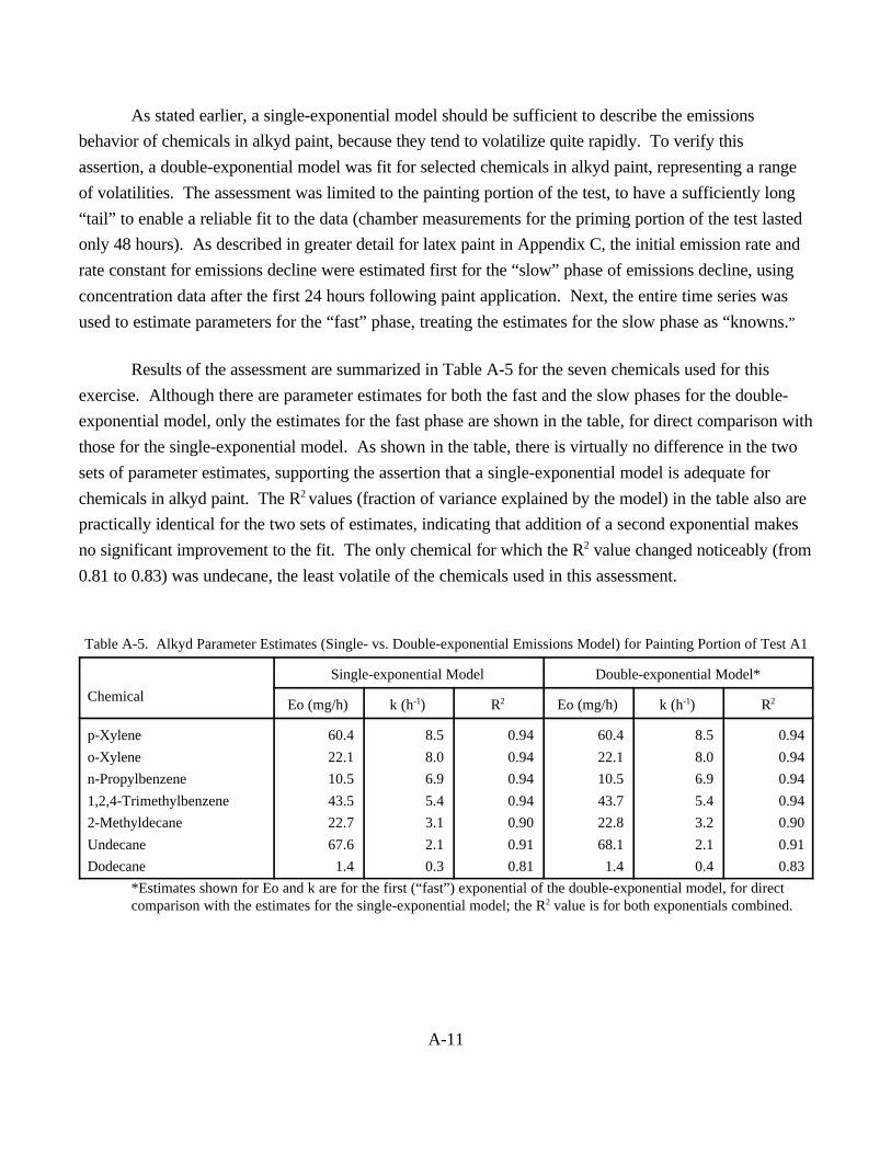
A-11
As stated earlier, a single-exponential model should be sufficient to describe the emissions
behavior of chemicals in alkyd paint, because they tend to volatilize quite rapidly. To verify this
assertion, a double-exponential model was fit for selected chemicals in alkyd paint, representing a range
of volatilities. The assessment was limited to the painting portion of the test, to have a sufficiently long
“tail” to enable a reliable fit to the data (chamber measurements for the priming portion of the test lasted
only 48 hours). As described in greater detail for latex paint in Appendix C, the initial emission rate and
rate constant for emissions decline were estimated first for the “slow” phase of emissions decline, using
concentration data after the first 24 hours following paint application. Next, the entire time series was
used to estimate parameters for the “fast” phase, treating the estimates for the slow phase as “knowns.”
Results of the assessment are summarized in Table A-5 for the seven chemicals used for this
exercise. Although there are parameter estimates for both the fast and the slow phases for the double-
exponential model, only the estimates for the fast phase are shown in the table, for direct comparison with
those for the single-exponential model. As shown in the table, there is virtually no difference in the two
sets of parameter estimates, supporting the assertion that a single-exponential model is adequate for
chemicals in alkyd paint. The R2 values (fraction of variance explained by the model) in the table also are
practically identical for the two sets of estimates, indicating that addition of a second exponential makes
no significant improvement to the fit. The only chemical for which the R2 value changed noticeably (from
0.81 to 0.83) was undecane, the least volatile of the chemicals used in this assessment.
Table A-5. Alkyd Parameter Estimates (Single- vs. Double-exponential Emissions Model) for Painting Portion of Test A1
Chemical
Single-exponential Model Double-exponential Model*
Eo (mg/h) k (h-1) R2 Eo (mg/h) k (h-1) R2
p-Xylene
o-Xylene
n-Propylbenzene
1,2,4-Trimethylbenzene
2-Methyldecane
Undecane
Dodecane
60.4
22.1
10.5
43.5
22.7
67.6
1.4
8.5
8.0
6.9
5.4
3.1
2.1
0.3
0.94
0.94
0.94
0.94
0.90
0.91
0.81
60.4
22.1
10.5
43.7
22.8
68.1
1.4
8.5
8.0
6.9
5.4
3.2
2.1
0.4
0.94
0.94
0.94
0.94
0.90
0.91
0.83
*Estimates shown for Eo and k are for the first (“fast”) exponential of the double-exponential model, for direct comparison with the estimates for the single-exponential model; the R2 value is for both exponentials combined.
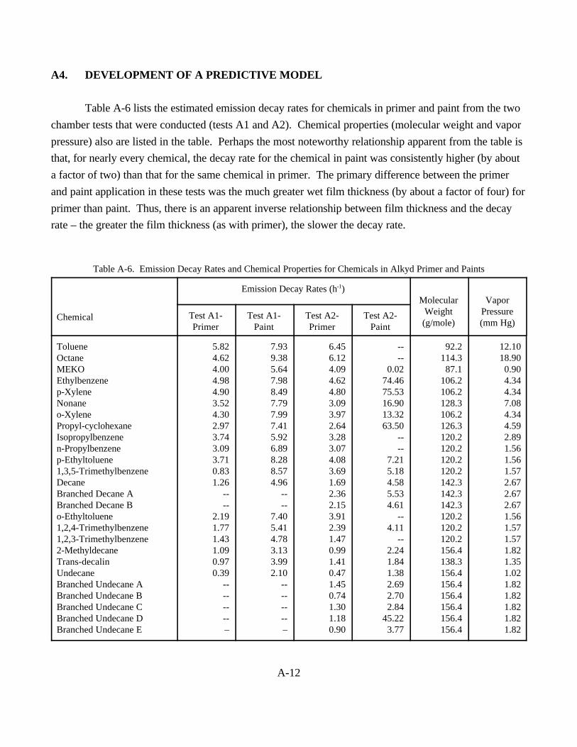
A-12
A4. DEVELOPMENT OF A PREDICTIVE MODEL
Table A-6 lists the estimated emission decay rates for chemicals in primer and paint from the two
chamber tests that were conducted (tests A1 and A2). Chemical properties (molecular weight and vapor
pressure) also are listed in the table. Perhaps the most noteworthy relationship apparent from the table is
that, for nearly every chemical, the decay rate for the chemical in paint was consistently higher (by about
a factor of two) than that for the same chemical in primer. The primary difference between the primer
and paint application in these tests was the much greater wet film thickness (by about a factor of four) for
primer than paint. Thus, there is an apparent inverse relationship between film thickness and the decay
rate – the greater the film thickness (as with primer), the slower the decay rate.
Table A-6. Emission Decay Rates and Chemical Properties for Chemicals in Alkyd Primer and Paints
Chemical
Emission Decay Rates (h-1)Molecular
Weight(g/mole)
VaporPressure(mm Hg)
Test A1-Primer
Test A1-Paint
Test A2-Primer
Test A2-Paint
TolueneOctaneMEKOEthylbenzenep-XyleneNonaneo-XylenePropyl-cyclohexaneIsopropylbenzenen-Propylbenzenep-Ethyltoluene1,3,5-TrimethylbenzeneDecaneBranched Decane ABranched Decane Bo-Ethyltoluene1,2,4-Trimethylbenzene1,2,3-Trimethylbenzene2-MethyldecaneTrans-decalinUndecaneBranched Undecane ABranched Undecane BBranched Undecane CBranched Undecane DBranched Undecane E
5.824.624.004.984.903.524.302.973.743.093.710.831.26
----
2.191.771.431.090.970.39
--------–
7.939.385.647.988.497.797.997.415.926.898.288.574.96
----
7.405.414.783.133.992.10
--------–
6.456.124.094.624.803.093.972.643.283.074.083.691.692.362.153.912.391.470.991.410.471.450.741.301.180.90
----
0.0274.4675.5316.9013.3263.50
----
7.215.184.585.534.61
--4.11
--2.241.841.382.692.702.84
45.223.77
92.2114.3
87.1106.2106.2128.3106.2126.3120.2120.2120.2120.2142.3142.3142.3120.2120.2120.2156.4138.3156.4156.4156.4156.4156.4156.4
12.1018.900.904.344.347.084.344.592.891.561.561.572.672.672.671.561.571.571.821.351.021.821.821.821.821.82
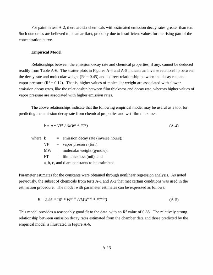
A-13
For paint in test A-2, there are six chemicals with estimated emission decay rates greater than ten.
Such outcomes are believed to be an artifact, probably due to insufficient values for the rising part of the
concentration curve.
Empirical Model
Relationships between the emission decay rate and chemical properties, if any, cannot be deduced
readily from Table A-6. The scatter plots in Figures A-4 and A-5 indicate an inverse relationship between
the decay rate and molecular weight (R2 = 0.45) and a direct relationship between the decay rate and
vapor pressure (R2 = 0.12). That is, higher values of molecular weight are associated with slower
emission decay rates, like the relationship between film thickness and decay rate, whereas higher values of
vapor pressure are associated with higher emission rates.
The above relationships indicate that the following empirical model may be useful as a tool for
predicting the emission decay rate from chemical properties and wet film thickness:
k = a * VPb / (MWc * FTd) (A-4)
where k = emission decay rate (inverse hours);
VP = vapor pressure (torr);
MW = molecular weight (g/mole);
FT = film thickness (mil); and
a, b, c, and d are constants to be estimated.
Parameter estimates for the constants were obtained through nonlinear regression analysis. As noted
previously, the subset of chemicals from tests A-1 and A-2 that met certain conditions was used in the
estimation procedure. The model with parameter estimates can be expressed as follows:
E = 2.95 * 109 * VP0.27 / (MW4.02 * FT0.58) (A-5)
This model provides a reasonably good fit to the data, with an R2 value of 0.86. The relatively strong
relationship between emission decay rates estimated from the chamber data and those predicted by the
empirical model is illustrated in Figure A-6.
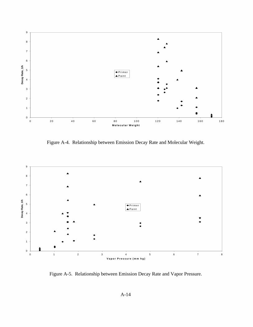
A-14
0
1
2
3
4
5
6
7
8
9
0 2 0 4 0 6 0 8 0 1 0 0 1 2 0 1 4 0 1 6 0 1 8 0
M o l e c u l a r W e i g h t
Dec
ay R
ate,
1/h
P r i m e r
Pa in t
0
1
2
3
4
5
6
7
8
9
0 1 2 3 4 5 6 7 8
V a p o r P r e s s u r e ( m m h g )
Dec
ay R
ate,
1/h
P r i m e r
P a i n t
Figure A-4. Relationship between Emission Decay Rate and Molecular Weight.
Figure A-5. Relationship between Emission Decay Rate and Vapor Pressure.
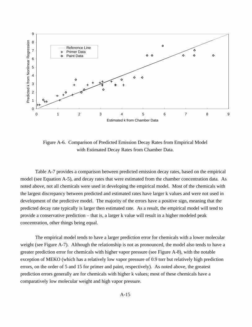
A-15
0
1
2
3
4
5
6
7
8
9
0 1 2 3 4 5 6 7 8 9
Estimated k from Chamber Data
Pre
dict
ed k
from
Non
linea
r R
egre
ssio
n
Reference LinePrimer DataPaint Data
Figure A-6. Comparison of Predicted Emission Decay Rates from Empirical Model
with Estimated Decay Rates from Chamber Data.
Table A-7 provides a comparison between predicted emission decay rates, based on the empirical
model (see Equation A-5), and decay rates that were estimated from the chamber concentration data. As
noted above, not all chemicals were used in developing the empirical model. Most of the chemicals with
the largest discrepancy between predicted and estimated rates have larger k values and were not used in
development of the predictive model. The majority of the errors have a positive sign, meaning that the
predicted decay rate typically is larger then estimated rate. As a result, the empirical model will tend to
provide a conservative prediction – that is, a larger k value will result in a higher modeled peak
concentration, other things being equal.
The empirical model tends to have a larger prediction error for chemicals with a lower molecular
weight (see Figure A-7). Although the relationship is not as pronounced, the model also tends to have a
greater prediction error for chemicals with higher vapor pressure (see Figure A-8), with the notable
exception of MEKO (which has a relatively low vapor pressure of 0.9 torr but relatively high prediction
errors, on the order of 5 and 15 for primer and paint, respectively). As noted above, the greatest
prediction errors generally are for chemicals with higher k values; most of these chemicals have a
comparatively low molecular weight and high vapor pressure.
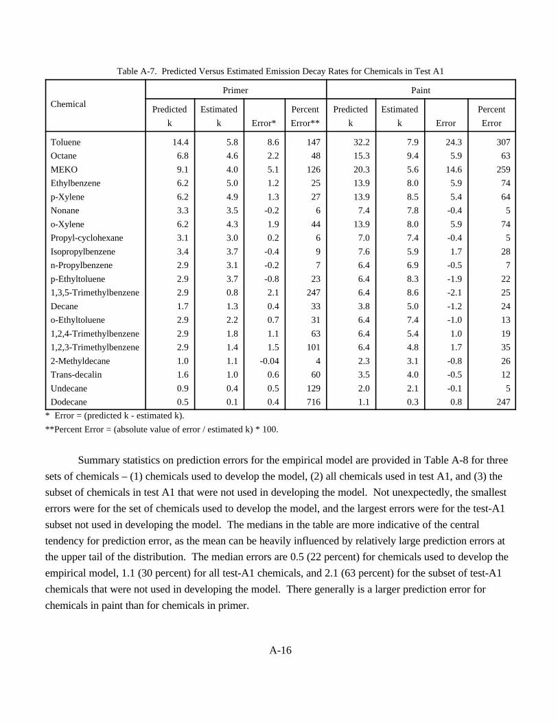
A-16
Table A-7. Predicted Versus Estimated Emission Decay Rates for Chemicals in Test A1
Chemical
Primer Paint
Predicted
k
Estimated
k Error*
Percent
Error**
Predicted
k
Estimated
k Error
Percent
Error
Toluene
Octane
MEKO
Ethylbenzene
p-Xylene
Nonane
o-Xylene
Propyl-cyclohexane
Isopropylbenzene
n-Propylbenzene
p-Ethyltoluene
1,3,5-Trimethylbenzene
Decane
o-Ethyltoluene
1,2,4-Trimethylbenzene
1,2,3-Trimethylbenzene
2-Methyldecane
Trans-decalin
Undecane
Dodecane
14.4
6.8
9.1
6.2
6.2
3.3
6.2
3.1
3.4
2.9
2.9
2.9
1.7
2.9
2.9
2.9
1.0
1.6
0.9
0.5
5.8
4.6
4.0
5.0
4.9
3.5
4.3
3.0
3.7
3.1
3.7
0.8
1.3
2.2
1.8
1.4
1.1
1.0
0.4
0.1
8.6
2.2
5.1
1.2
1.3
-0.2
1.9
0.2
-0.4
-0.2
-0.8
2.1
0.4
0.7
1.1
1.5
-0.04
0.6
0.5
0.4
147
48
126
25
27
6
44
6
9
7
23
247
33
31
63
101
4
60
129
716
32.2
15.3
20.3
13.9
13.9
7.4
13.9
7.0
7.6
6.4
6.4
6.4
3.8
6.4
6.4
6.4
2.3
3.5
2.0
1.1
7.9
9.4
5.6
8.0
8.5
7.8
8.0
7.4
5.9
6.9
8.3
8.6
5.0
7.4
5.4
4.8
3.1
4.0
2.1
0.3
24.3
5.9
14.6
5.9
5.4
-0.4
5.9
-0.4
1.7
-0.5
-1.9
-2.1
-1.2
-1.0
1.0
1.7
-0.8
-0.5
-0.1
0.8
307
63
259
74
64
5
74
5
28
7
22
25
24
13
19
35
26
12
5
247
* Error = (predicted k - estimated k).
**Percent Error = (absolute value of error / estimated k) * 100.
Summary statistics on prediction errors for the empirical model are provided in Table A-8 for three
sets of chemicals – (1) chemicals used to develop the model, (2) all chemicals used in test A1, and (3) the
subset of chemicals in test A1 that were not used in developing the model. Not unexpectedly, the smallest
errors were for the set of chemicals used to develop the model, and the largest errors were for the test-A1
subset not used in developing the model. The medians in the table are more indicative of the central
tendency for prediction error, as the mean can be heavily influenced by relatively large prediction errors at
the upper tail of the distribution. The median errors are 0.5 (22 percent) for chemicals used to develop the
empirical model, 1.1 (30 percent) for all test-A1 chemicals, and 2.1 (63 percent) for the subset of test-A1
chemicals that were not used in developing the model. There generally is a larger prediction error for
chemicals in paint than for chemicals in primer.
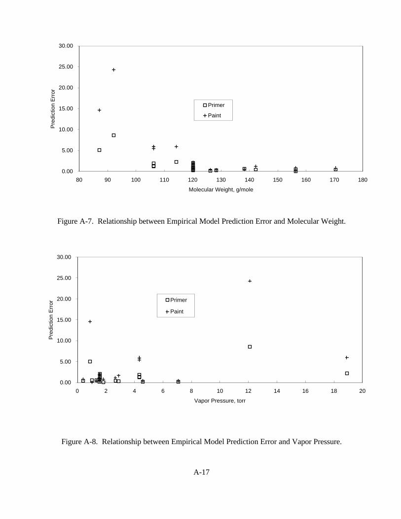
A-17
0.00
5.00
10.00
15.00
20.00
25.00
30.00
80 90 100 110 120 130 140 150 160 170 180
Molecular Weight, g/mole
Pre
dict
ion
Err
or
Primer
Paint
0.00
5.00
10.00
15.00
20.00
25.00
30.00
0 2 4 6 8 10 12 14 16 18 20
Vapor Pressure, torr
Pre
dict
ion
Err
or
Primer
Paint
Figure A-7. Relationship between Empirical Model Prediction Error and Molecular Weight.
Figure A-8. Relationship between Empirical Model Prediction Error and Vapor Pressure.
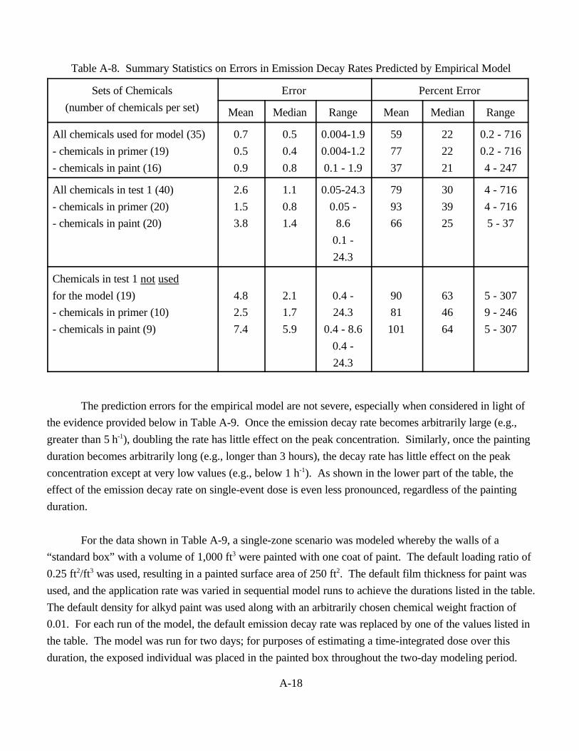
A-18
Table A-8. Summary Statistics on Errors in Emission Decay Rates Predicted by Empirical Model
Sets of Chemicals
(number of chemicals per set)
Error Percent Error
Mean Median Range Mean Median Range
All chemicals used for model (35)
- chemicals in primer (19)
- chemicals in paint (16)
0.7
0.5
0.9
0.5
0.4
0.8
0.004-1.9
0.004-1.2
0.1 - 1.9
59
77
37
22
22
21
0.2 - 716
0.2 - 716
4 - 247
All chemicals in test 1 (40)
- chemicals in primer (20)
- chemicals in paint (20)
2.6
1.5
3.8
1.1
0.8
1.4
0.05-24.3
0.05 -
8.6
0.1 -
24.3
79
93
66
30
39
25
4 - 716
4 - 716
5 - 37
Chemicals in test 1 not used
for the model (19)
- chemicals in primer (10)
- chemicals in paint (9)
4.8
2.5
7.4
2.1
1.7
5.9
0.4 -
24.3
0.4 - 8.6
0.4 -
24.3
90
81
101
63
46
64
5 - 307
9 - 246
5 - 307
The prediction errors for the empirical model are not severe, especially when considered in light of
the evidence provided below in Table A-9. Once the emission decay rate becomes arbitrarily large (e.g.,
greater than 5 h-1), doubling the rate has little effect on the peak concentration. Similarly, once the painting
duration becomes arbitrarily long (e.g., longer than 3 hours), the decay rate has little effect on the peak
concentration except at very low values (e.g., below 1 h-1). As shown in the lower part of the table, the
effect of the emission decay rate on single-event dose is even less pronounced, regardless of the painting
duration.
For the data shown in Table A-9, a single-zone scenario was modeled whereby the walls of a
“standard box” with a volume of 1,000 ft3 were painted with one coat of paint. The default loading ratio of
0.25 ft2/ft3 was used, resulting in a painted surface area of 250 ft2. The default film thickness for paint was
used, and the application rate was varied in sequential model runs to achieve the durations listed in the table.
The default density for alkyd paint was used along with an arbitrarily chosen chemical weight fraction of
0.01. For each run of the model, the default emission decay rate was replaced by one of the values listed in
the table. The model was run for two days; for purposes of estimating a time-integrated dose over this
duration, the exposed individual was placed in the painted box throughout the two-day modeling period.
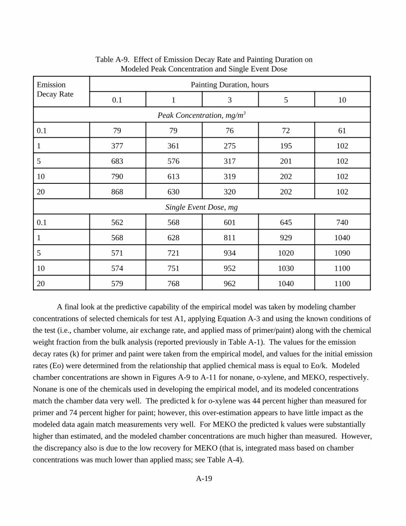
A-19
Table A-9. Effect of Emission Decay Rate and Painting Duration onModeled Peak Concentration and Single Event Dose
EmissionDecay Rate
Painting Duration, hours
0.1 1 3 5 10
Peak Concentration, mg/m3
0.1 79 79 76 72 61
1 377 361 275 195 102
5 683 576 317 201 102
10 790 613 319 202 102
20 868 630 320 202 102
Single Event Dose, mg
0.1 562 568 601 645 740
1 568 628 811 929 1040
5 571 721 934 1020 1090
10 574 751 952 1030 1100
20 579 768 962 1040 1100
A final look at the predictive capability of the empirical model was taken by modeling chamber
concentrations of selected chemicals for test A1, applying Equation A-3 and using the known conditions of
the test (i.e., chamber volume, air exchange rate, and applied mass of primer/paint) along with the chemical
weight fraction from the bulk analysis (reported previously in Table A-1). The values for the emission
decay rates (k) for primer and paint were taken from the empirical model, and values for the initial emission
rates (Eo) were determined from the relationship that applied chemical mass is equal to Eo/k. Modeled
chamber concentrations are shown in Figures A-9 to A-11 for nonane, o-xylene, and MEKO, respectively.
Nonane is one of the chemicals used in developing the empirical model, and its modeled concentrations
match the chamber data very well. The predicted k for o-xylene was 44 percent higher than measured for
primer and 74 percent higher for paint; however, this over-estimation appears to have little impact as the
modeled data again match measurements very well. For MEKO the predicted k values were substantially
higher than estimated, and the modeled chamber concentrations are much higher than measured. However,
the discrepancy also is due to the low recovery for MEKO (that is, integrated mass based on chamber
concentrations was much lower than applied mass; see Table A-4).
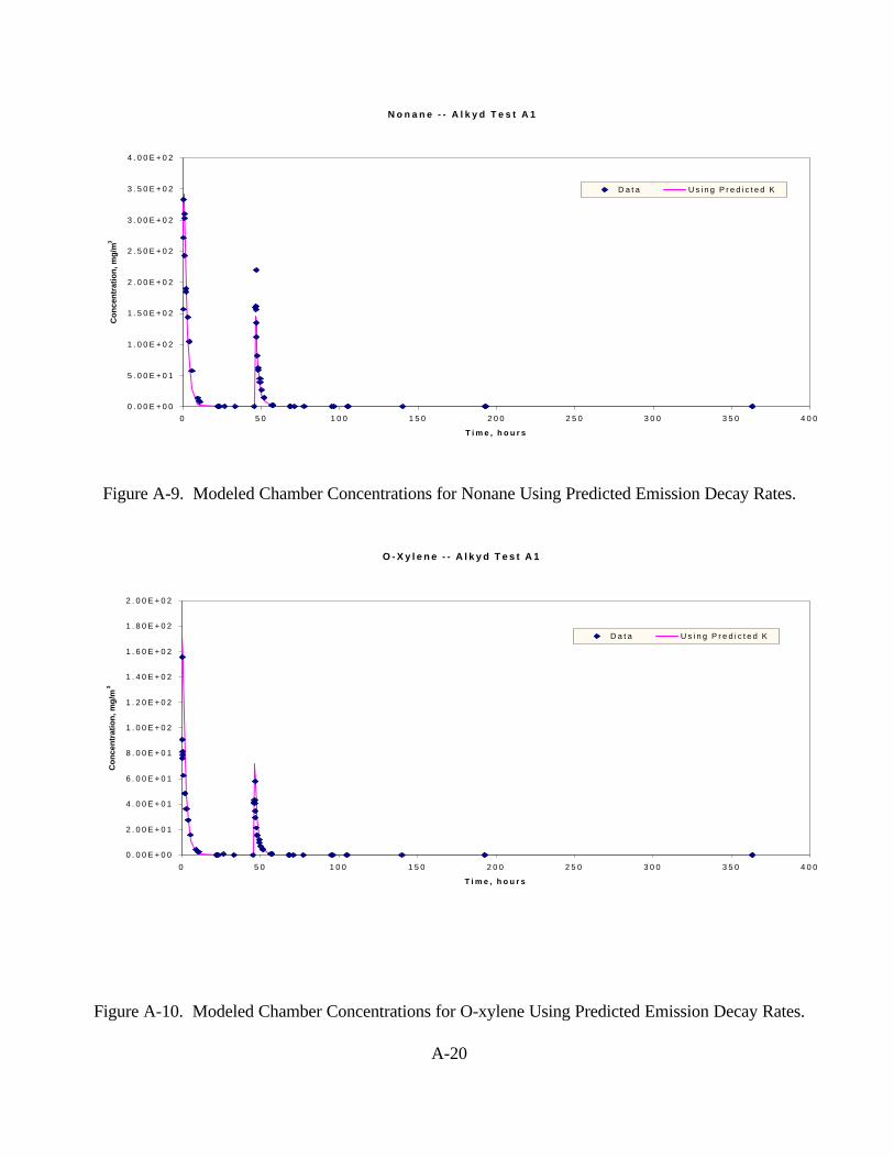
A-20
N o n a n e - - A l k y d T e s t A 1
0 . 0 0 E + 0 0
5 . 0 0 E + 0 1
1 . 0 0 E + 0 2
1 . 5 0 E + 0 2
2 . 0 0 E + 0 2
2 . 5 0 E + 0 2
3 . 0 0 E + 0 2
3 . 5 0 E + 0 2
4 . 0 0 E + 0 2
0 5 0 1 0 0 1 5 0 2 0 0 2 5 0 3 0 0 3 5 0 4 0 0
T i m e , h o u r s
Co
nce
ntr
atio
n, m
g/m
3
D a t a U s i n g P r e d i c t e d K
O - X y l e n e - - A l k y d T e s t A 1
0 . 0 0 E + 0 0
2 . 0 0 E + 0 1
4 . 0 0 E + 0 1
6 . 0 0 E + 0 1
8 . 0 0 E + 0 1
1 . 0 0 E + 0 2
1 . 2 0 E + 0 2
1 . 4 0 E + 0 2
1 . 6 0 E + 0 2
1 . 8 0 E + 0 2
2 . 0 0 E + 0 2
0 5 0 1 0 0 1 5 0 2 0 0 2 5 0 3 0 0 3 5 0 4 0 0
T i m e , h o u r s
Co
nce
ntr
atio
n, m
g/m
3
D a t a U s i n g P r e d i c t e d K
Figure A-9. Modeled Chamber Concentrations for Nonane Using Predicted Emission Decay Rates.
Figure A-10. Modeled Chamber Concentrations for O-xylene Using Predicted Emission Decay Rates.
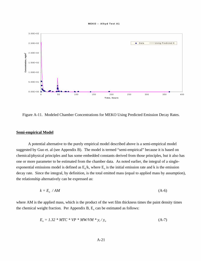
A-21
M E K O - - A l k y d T e s t A 1
0 . 0 0 E + 0 0
5 . 0 0 E + 0 1
1 . 0 0 E + 0 2
1 . 5 0 E + 0 2
2 . 0 0 E + 0 2
2 . 5 0 E + 0 2
3 . 0 0 E + 0 2
0 5 0 1 0 0 1 5 0 2 0 0 2 5 0 3 0 0 3 5 0 4 0 0
T i m e , h o u r s
Co
nce
ntr
atio
n, m
g/m
3
D a t a U s i n g P r e d i c t e d K
Figure A-11. Modeled Chamber Concentrations for MEKO Using Predicted Emission Decay Rates.
Semi-empirical Model
A potential alternative to the purely empirical model described above is a semi-empirical model
suggested by Guo et. al (see Appendix B). The model is termed “semi-empirical” because it is based on
chemical/physical principles and has some embedded constants derived from those principles, but it also has
one or more parameter to be estimated from the chamber data. As noted earlier, the integral of a single-
exponential emissions model is defined as Eo/k, where Eo is the initial emission rate and k is the emission
decay rate. Since the integral, by definition, is the total emitted mass (equal to applied mass by assumption),
the relationship alternatively can be expressed as:
k = Eo / AM (A-6)
where AM is the applied mass, which is the product of the wet film thickness times the paint density times
the chemical weight fraction. Per Appendix B, Eo can be estimated as follows:
Eo = 1.32 * MTC * VP * MW/VM * yi / yo (A-7)
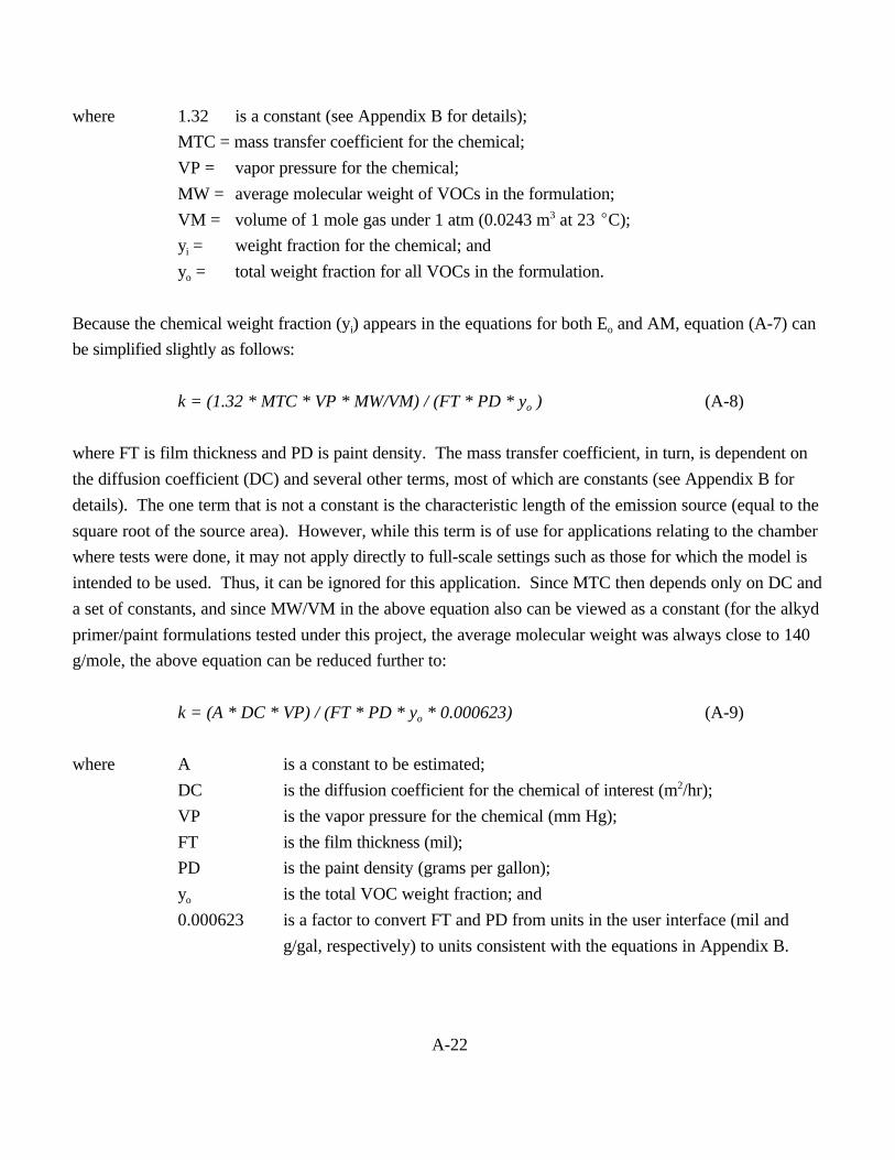
A-22
where 1.32 is a constant (see Appendix B for details);
MTC = mass transfer coefficient for the chemical;
VP = vapor pressure for the chemical;
MW = average molecular weight of VOCs in the formulation;
VM = volume of 1 mole gas under 1 atm (0.0243 m3 at 23 EC);
yi = weight fraction for the chemical; and
yo = total weight fraction for all VOCs in the formulation.
Because the chemical weight fraction (yi) appears in the equations for both Eo and AM, equation (A-7) can
be simplified slightly as follows:
k = (1.32 * MTC * VP * MW/VM) / (FT * PD * yo ) (A-8)
where FT is film thickness and PD is paint density. The mass transfer coefficient, in turn, is dependent on
the diffusion coefficient (DC) and several other terms, most of which are constants (see Appendix B for
details). The one term that is not a constant is the characteristic length of the emission source (equal to the
square root of the source area). However, while this term is of use for applications relating to the chamber
where tests were done, it may not apply directly to full-scale settings such as those for which the model is
intended to be used. Thus, it can be ignored for this application. Since MTC then depends only on DC and
a set of constants, and since MW/VM in the above equation also can be viewed as a constant (for the alkyd
primer/paint formulations tested under this project, the average molecular weight was always close to 140
g/mole, the above equation can be reduced further to:
k = (A * DC * VP) / (FT * PD * yo * 0.000623) (A-9)
where A is a constant to be estimated;
DC is the diffusion coefficient for the chemical of interest (m2/hr);
VP is the vapor pressure for the chemical (mm Hg);
FT is the film thickness (mil);
PD is the paint density (grams per gallon);
yo is the total VOC weight fraction; and
0.000623 is a factor to convert FT and PD from units in the user interface (mil and
g/gal, respectively) to units consistent with the equations in Appendix B.
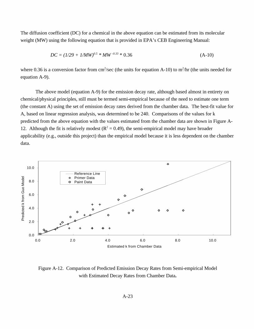
A-23
0.0
2.0
4.0
6.0
8.0
10.0
0.0 2.0 4.0 6.0 8.0 10.0
Estimated k from Chamber Data
Pre
dict
ed k
from
Guo
Mod
el
Reference LinePrimer DataPaint Data
The diffusion coefficient (DC) for a chemical in the above equation can be estimated from its molecular
weight (MW) using the following equation that is provided in EPA’s CEB Engineering Manual:
DC = (1/29 + 1/MW)0.5 * MW -0.33 * 0.36 (A-10)
where 0.36 is a conversion factor from cm2/sec (the units for equation A-10) to m2/hr (the units needed for
equation A-9).
The above model (equation A-9) for the emission decay rate, although based almost in entirety on
chemical/physical principles, still must be termed semi-empirical because of the need to estimate one term
(the constant A) using the set of emission decay rates derived from the chamber data. The best-fit value for
A, based on linear regression analysis, was determined to be 240. Comparisons of the values for k
predicted from the above equation with the values estimated from the chamber data are shown in Figure A-
12. Although the fit is relatively modest (R2 = 0.49), the semi-empirical model may have broader
applicability (e.g., outside this project) than the empirical model because it is less dependent on the chamber
data.
Figure A-12. Comparison of Predicted Emission Decay Rates from Semi-empirical Model
with Estimated Decay Rates from Chamber Data.
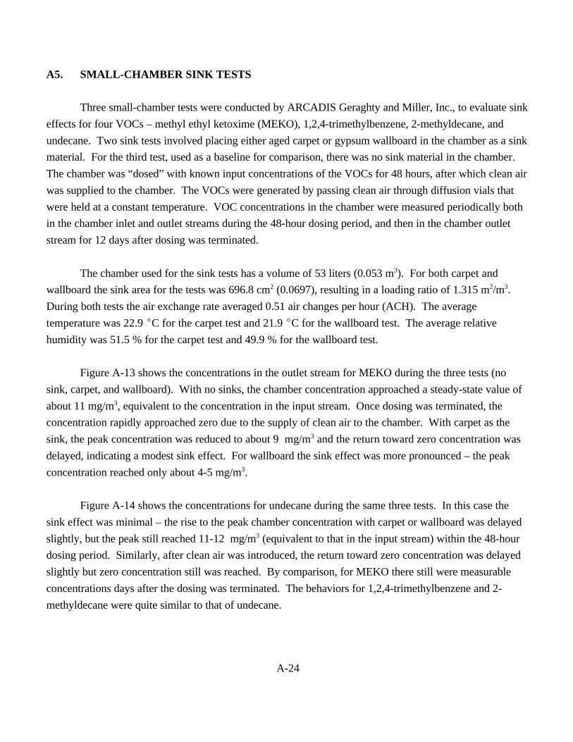
A-24
A5. SMALL-CHAMBER SINK TESTS
Three small-chamber tests were conducted by ARCADIS Geraghty and Miller, Inc., to evaluate sink
effects for four VOCs – methyl ethyl ketoxime (MEKO), 1,2,4-trimethylbenzene, 2-methyldecane, and
undecane. Two sink tests involved placing either aged carpet or gypsum wallboard in the chamber as a sink
material. For the third test, used as a baseline for comparison, there was no sink material in the chamber.
The chamber was “dosed” with known input concentrations of the VOCs for 48 hours, after which clean air
was supplied to the chamber. The VOCs were generated by passing clean air through diffusion vials that
were held at a constant temperature. VOC concentrations in the chamber were measured periodically both
in the chamber inlet and outlet streams during the 48-hour dosing period, and then in the chamber outlet
stream for 12 days after dosing was terminated.
The chamber used for the sink tests has a volume of 53 liters (0.053 m3). For both carpet and
wallboard the sink area for the tests was 696.8 cm2 (0.0697), resulting in a loading ratio of 1.315 m2/m3.
During both tests the air exchange rate averaged 0.51 air changes per hour (ACH). The average
temperature was 22.9 EC for the carpet test and 21.9 EC for the wallboard test. The average relative
humidity was 51.5 % for the carpet test and 49.9 % for the wallboard test.
Figure A-13 shows the concentrations in the outlet stream for MEKO during the three tests (no
sink, carpet, and wallboard). With no sinks, the chamber concentration approached a steady-state value of
about 11 mg/m3, equivalent to the concentration in the input stream. Once dosing was terminated, the
concentration rapidly approached zero due to the supply of clean air to the chamber. With carpet as the
sink, the peak concentration was reduced to about 9 mg/m3 and the return toward zero concentration was
delayed, indicating a modest sink effect. For wallboard the sink effect was more pronounced – the peak
concentration reached only about 4-5 mg/m3.
Figure A-14 shows the concentrations for undecane during the same three tests. In this case the
sink effect was minimal – the rise to the peak chamber concentration with carpet or wallboard was delayed
slightly, but the peak still reached 11-12 mg/m3 (equivalent to that in the input stream) within the 48-hour
dosing period. Similarly, after clean air was introduced, the return toward zero concentration was delayed
slightly but zero concentration still was reached. By comparison, for MEKO there still were measurable
concentrations days after the dosing was terminated. The behaviors for 1,2,4-trimethylbenzene and 2-
methyldecane were quite similar to that of undecane.
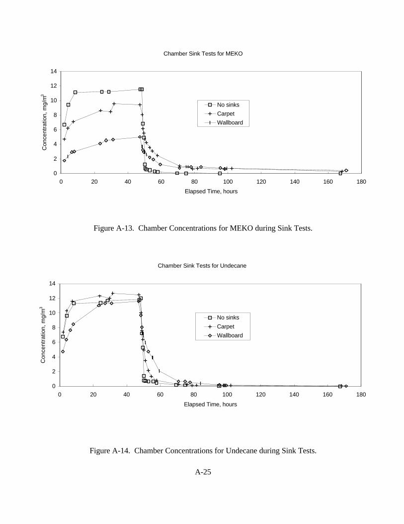
A-25
Chamber Sink Tests for MEKO
0
2
4
6
8
10
12
14
0 20 40 60 80 100 120 140 160 180
Elapsed Time, hours
Con
cent
ratio
n, m
g/m
3
No sinks
Carpet
Wallboard
Chamber Sink Tests for Undecane
0
2
4
6
8
10
12
14
0 20 40 60 80 100 120 140 160 180
Elapsed Time, hours
Con
cent
ratio
n, m
g/m
3
No sinks
Carpet
Wallboard
Figure A-13. Chamber Concentrations for MEKO during Sink Tests.
Figure A-14. Chamber Concentrations for Undecane during Sink Tests.
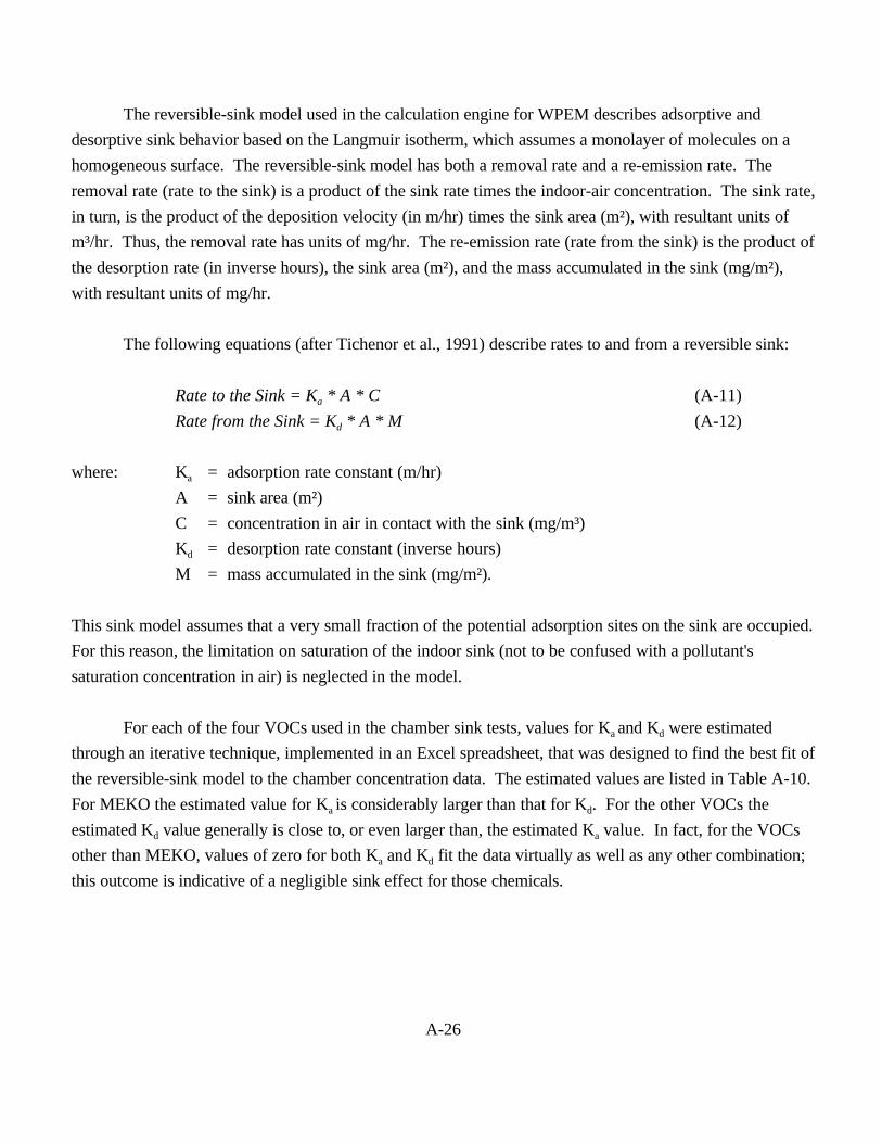
A-26
The reversible-sink model used in the calculation engine for WPEM describes adsorptive and
desorptive sink behavior based on the Langmuir isotherm, which assumes a monolayer of molecules on a
homogeneous surface. The reversible-sink model has both a removal rate and a re-emission rate. The
removal rate (rate to the sink) is a product of the sink rate times the indoor-air concentration. The sink rate,
in turn, is the product of the deposition velocity (in m/hr) times the sink area (m²), with resultant units of
m³/hr. Thus, the removal rate has units of mg/hr. The re-emission rate (rate from the sink) is the product of
the desorption rate (in inverse hours), the sink area (m²), and the mass accumulated in the sink (mg/m²),
with resultant units of mg/hr.
The following equations (after Tichenor et al., 1991) describe rates to and from a reversible sink:
Rate to the Sink = Ka * A * C (A-11)
Rate from the Sink = Kd * A * M (A-12)
where: Ka = adsorption rate constant (m/hr)
A = sink area (m²)
C = concentration in air in contact with the sink (mg/m³)
Kd = desorption rate constant (inverse hours)
M = mass accumulated in the sink (mg/m²).
This sink model assumes that a very small fraction of the potential adsorption sites on the sink are occupied.
For this reason, the limitation on saturation of the indoor sink (not to be confused with a pollutant's
saturation concentration in air) is neglected in the model.
For each of the four VOCs used in the chamber sink tests, values for Ka and Kd were estimated
through an iterative technique, implemented in an Excel spreadsheet, that was designed to find the best fit of
the reversible-sink model to the chamber concentration data. The estimated values are listed in Table A-10.
For MEKO the estimated value for Ka is considerably larger than that for Kd. For the other VOCs the
estimated Kd value generally is close to, or even larger than, the estimated Ka value. In fact, for the VOCs
other than MEKO, values of zero for both Ka and Kd fit the data virtually as well as any other combination;
this outcome is indicative of a negligible sink effect for those chemicals.
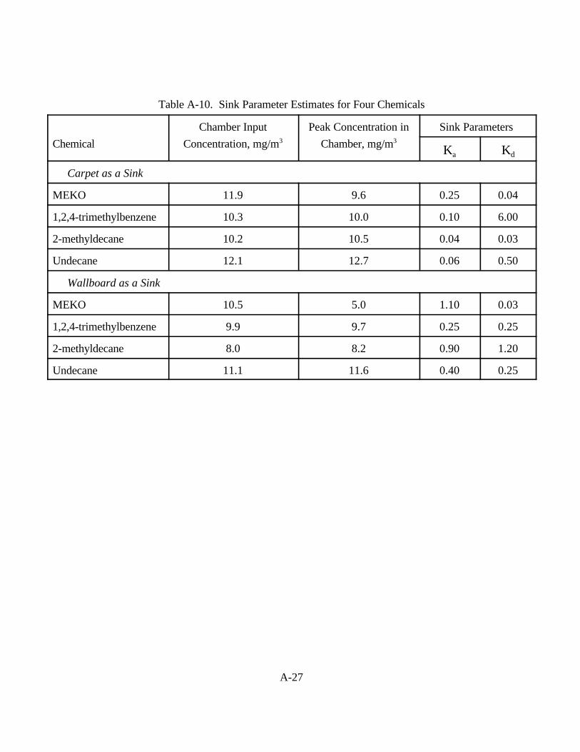
A-27
Table A-10. Sink Parameter Estimates for Four Chemicals
Chemical
Chamber Input
Concentration, mg/m3
Peak Concentration in
Chamber, mg/m3
Sink Parameters
Ka Kd
Carpet as a Sink
MEKO 11.9 9.6 0.25 0.04
1,2,4-trimethylbenzene 10.3 10.0 0.10 6.00
2-methyldecane 10.2 10.5 0.04 0.03
Undecane 12.1 12.7 0.06 0.50
Wallboard as a Sink
MEKO 10.5 5.0 1.10 0.03
1,2,4-trimethylbenzene 9.9 9.7 0.25 0.25
2-methyldecane 8.0 8.2 0.90 1.20
Undecane 11.1 11.6 0.40 0.25

APPENDIX B
PAPER ON EMISSIONS MODEL FOR ALKYD PAINTS(published in Atmospheric Environment, Vol. 33, No. 8, pp. 1205-1215)
B-1
Estimation of the Rate of VOC EmissionsFrom Solvent-Based Indoor Coating Materials
Based on Product Formulation
Zhishi Guo, John C. S. Chang, and Leslie E. SparksU.S. Environmental Protection Agency
National Risk Management Research LaboratoryIndoor Environment Management Branch, MD-54
Research Triangle Park, NC 27711, U.S.A.
Roy C. FortmannARCADIS Geraghty & Miller Company
P. O. Box 13109Research Triangle Park, NC 27709, U.S.A.
Published in
Atmospheric Environment
Vol. 33, No. 8, pp 1205-1215
B-2
ABSTRACT
Two computational methods are proposed for estimation of the emission rate of volatile
organic compounds (VOCs) from solvent-based indoor coating materials based on the knowledge of
product formulation. The first method utilizes two previously developed mass transfer models with
two key parameters -- the total vapor pressure and the average molecular weight for total volatile
organic compounds (TVOCs) -- being estimated based on the VOC contents in the product. The
second method is based on a simple, first-order decay model with its parameters being estimated
from the properties of both the source and the environment. All the model parameters can be readily
obtained. Detailed procedures for computing the key parameters are described by using examples.
The predictive errors were evaluated with small chamber data, and the results were satisfactory.
Thus, the proposed methods provide a way to predict the VOC emissions in the indoor environment
without having to conduct costly chamber testing. The two proposed methods work for both
TVOCs and individual VOCs. Pros and cons for each method are discussed.
Key Words
indoor air, emissions, volatile organic compounds, model, coating materials
B-3
1. INTRODUCTION
Solvent-based interior coating materials have long been recognized as a major source of
volatile organic compounds (VOCs) in the indoor environment (Sterling, 1984). They usually
contain more than 25 percent of the solvent that will be released into the air during the drying period.
The most commonly used solvent in these products is mineral spirits -- a type of petroleum distillate
consisting of aliphatic hydrocarbons with a trace amount of aromatics (Howe-Grant, 1996). Other
VOCs are sometimes added to the formulation to enhance its performance, including oxygenated
hydrocarbons (such as alcohols), nitrogenated hydrocarbons (such as methyl ethyl ketoxime), and
other solvents (such as toluene). Some of the solvent components are identified as hazardous air
pollutants (HAPs) in the Clean Air Act Amendments of 1990 (U. S. Public Law 101-549, 1990).
The increased exposure to those HAPs and the subsequent health risk are of special concern when
solvent-based coatings are used in the indoor environment.
Small environmental chambers have been used to determine the VOC emissions from interior
coatings (ASTM, 1995a). The cost of chamber testing could be very high because characterization
of emission patterns requires multiple samples over time and this is especially true when the
emissions of individual VOCs are to be quantified. A tremendous amount of time and resources can
be saved if the emission rates can be predicted based on the properties of the source and those of the
environment.
This paper presents two methods that can be used to predict the emissions of TVOCs and
individual VOCs from solvent-based indoor coatings. They are both based on gas-phase mass
transfer theories but differ in complexity.
The proposed methods should be useful in exposure estimation and risk assessment for they
can predict indoor VOC emissions with reasonable accuracy without having to rely on costly
chamber testing. These methods should also be useful to manufacturers in developing low-emission
products for, once the concentrations of predominant VOCs in a product are known, all the
information needed to predict the VOC emission rates is known.
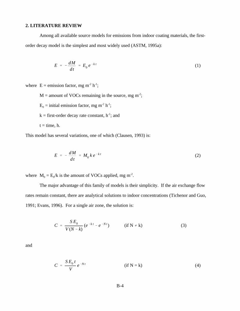
B-4
2. LITERATURE REVIEW
Among all available source models for emissions from indoor coating materials, the first-
order decay model is the simplest and most widely used (ASTM, 1995a):
(1)E ' &dMdt
' E0 e &k t
where E = emission factor, mg m-2 h-1;
M = amount of VOCs remaining in the source, mg m-2;
E0 = initial emission factor, mg m-2 h-1;
k = first-order decay rate constant, h-1; and
t = time, h.
This model has several variations, one of which (Clausen, 1993) is:
(2)E ' &dMdt
' M0 k e &k t
where M0 = E0/k is the amount of VOCs applied, mg m-2.
The major advantage of this family of models is their simplicity. If the air exchange flow
rates remain constant, there are analytical solutions to indoor concentrations (Tichenor and Guo,
1991; Evans, 1996). For a single air zone, the solution is:
(if N … k) (3)C 'S E0
V (N & k)(e &k t & e &N t )
and
(if N = k) (4)C 'S E0 t
Ve &N t
B-5
where C = indoor concentration, mg m-3;
S = source area, m²;
V = room volume, m³; and
N = air exchange rate, h-1.
The first-order decay model has two major drawbacks, however. First, estimation of
parameters E0 and k often relies on costly chamber tests. Second, as an empirical model, it is
difficult to scale-up.
Efforts have been made to overcome these problems. Clausen (1993) found that, for a given
product, the decay rate constant k is inversely proportional to the wet film thickness:
(5)k 'kE1
è
where è = wet film thickness, µm; and
kE1 = decay rate constant for an evaporative source with wet film thickness of 1 µm, µm h -1.
This equation provides a way to adjust k when the wet film thickness changes.
Chang and Guo (1994) reported that, for individual VOCs in a given product, the decay rate
constant k can be related to their vapor pressure P:
(6)k1
k2
'P1
P2
Such correlation allows estimation of k for one compound relative to another.
Another development allows estimation of k based on the drying time of the solvent (Evans,
1996). Integrating Equation 2 yields:
(7)M ' M0 e &k t
B-6
If the drying time, tD, is defined as the time needed for 90 percent of the solvent to evaporate, then
Equation 7 becomes:
(8)0.1 M0 ' M0 e&k tD
or
(9)k ' &ln(0.1)
tD
Two mass transfer models were introduced to solve the scale-up problem. One, known as
the VB model, is for TVOC (Tichenor, et al., 1993) and the other, known as the VBX model, for
individual VOCs (Guo, et al., 1998). These two models are discussed further in the following
section.
The gas-phase mass transfer coefficient, which appears in both the VB and VBX models,
plays an important role in controlling the rate of VOC emissions from wet sources (Guo, et al.,
1996). Two theoretical models have been developed to estimate this parameter in indoor
environments (Sparks et al., 1996; Zhang, et al., 1996). Sparks et al. proposed a simple formula
based on correlation of the Nusselt and Reynolds. Zhang, et al. reported a slightly more complex
formula, which takes into consideration such additional factors as the boundary layer flow condition
and the wall shear stress.
To date, no reported methods allow estimation of emission rates for either TVOCs or
individual VOCs based on information about the product formulation. The two methods proposed in
this paper attempt to fill this gap.
3. DESCRIPTION OF THE METHODS
3.1 Method 1
Method 1 utilizes the VB model (Tichenor, et al., 1993) for TVOCs (Equation 10) and a
modified VBX model for individual VOCs (Equation 11):
B-7
(10)E ' km (Cv0
MT
MT0
& C)
where km = gas-phase mass transfer coefficient for TVOCs, m h-1;
Cv0 = initial airborne TVOC concentration at air/source interface, mg m-3, based on the total
vapor pressure of the TVOCs;
MT = amount of TVOCs remaining in the source, mg m-2;
MT0 = amount of TVOCs applied, mg m-2; and
C = TVOC concentration in the bulk air, mg m-3.
(11)Ei ' kmi (Cvi
Mi
MT
mmi
& Ci )
where Ei = emission factor for component i, mg m-2 h-1;
kmi = gas-phase mass transfer coefficient for component i, m h-1;
Cvi = airborne concentration of component i at air/source interface, mg m-3, based on the
vapor pressure of component i;
Mi = amount of component i remaining in the source, mg m-2;
= average molecular weight for the organic solvent, g mole-1; m
mi = molecular weight for component i, g mole-1; and
Ci = concentration of component i in the bulk air, mg m-3.
The term is the approximate molar fraction of component i in the solvent mixture. Mi
MT
mmi
Equation 11 is equivalent to the original VBX model (Guo, et al., 1998) but easier to use because it
does not require any unit conversion between (mg m-3) and (mole m-3) for the concentration.
When the emission factor is estimated from the VOC contents in the formulation, it is more
convenient to convert Cv0 and Cvi to commonly used pressure units such as (mm Hg):
B-8
(12)Cv0 ' 103P0
760m
vm
(13)Cvi ' 103Pi
760
mi
vm
where P0 = total vapor pressure for TVOCs, mm Hg;
Pi = vapor pressure for the pure component i, mm Hg; and
vm = volume of 1 mole gas under 1 atm, m³ (vm = 0.0243 m³ at 23°C).
Substituting Equation 12 into 10 and Equation 13 into 11:
(14)E ' km (1.32 P0mvm
MT
MT0
& C)
(15)Ei ' kmi (1.32 Pimvm
Mi
MT
& Ci)
The room concentration model consists of two differential equations for TVOCs (Equations
16 and 17) and an additional two for each individual VOC (Equations 18 and 19):
(16)dC
dt'
S E
V& N C
(17)dMT
dt' & E
(18)dCi
dt'
S Ei
V& N Ci
(19)dMi
d t' & Ei
B-9
where E and Ei are from Equations 14 and 15, respectively. The most common initial conditions for
Equations 16-19 are: C = 0, Ci = 0, MT = MT0, and Mi = Mi0 when t = 0. The amount of TVOCs and
individual VOCs initially applied, MT0 and Mi0, can be calculated from:
(20)MT0 ' è d y0
(21)Mi0 ' è d yi
where è = wet film thickness, m;
d = product density, g m-3;
y0 = TVOC content in the product, mg g-1; and
yi = content of component i in the product, mg g-1.
Equations 20 and 21 are also valid when è is in µm and d in kg L -1.
This method requires knowledge of total vapor pressure (P0) and average molecular weight
( ) for TVOCs, and mass transfer coefficients (km and kmi). Methods to estimate these parametersm
are described in Sections 4.2-4.4.
3.2 Method 2
In the second proposed method, the first-order decay model (Equation 1) -- the simplest
possible source model for decaying sources -- is adopted, with the two model parameters, E0 and k,
being estimated from the two mass transfer models described in the previous section by making
certain approximations. At t = 0, Equations 14 and 15 become:
(22)E0 ' km (1.32 P0mvm
MT0
MT0
& 0) ' 1.32 km P0mvm
(23)E0i ' kmi (1.32 Pimvm
Mi0
MT0
& 0) ' 1.32 kmi Pimvm
Mi0
MT0
B-10
Since , Equation 23 can be changed to:M
M
y
y
io
T
i
0 0=
(24)E0i ' 1.32 kmi Pimvm
yi
y0
From Equations 1 and 2, the first-order decay rate constant for TVOCs can be calculated from;
(25)k 'E0
MT0
Substituting Equation 20 into 25:
(26)k 'E0
è d y0
For an individual VOC, the decay rate constant (ki) can be derived in a similar manner:
(27)ki 'E0i
è d yi
Once E0 and k or E0i and ki are obtained, Equations 3 and 4 can be used to calculate room
concentrations.
B-11
4. PARAMETER ESTIMATION
4.1 Overview
The source models used in the two methods are summarized in Table 1. Table 2 is a list of all
parameters required to compute indoor VOC concentrations with the two proposed methods: the
first three parameters are properties of the environment, and the rest are properties of the source. It
is fair to say that all the parameters can be readily obtained except P0, , km and kmi. Methods form
estimating these parameters are discussed below.
4.2 Estimation of Total Vapor Pressure for TVOC (P0) from VOC Contents in the Product
To date, parameter P0 can only be determined by experiment (an example is described
below). An alternative method proposed here is to estimate P0 based on the contents of major VOCs
in the solvent. If we assume that the behavior of the solvent is close to an ideal solution, the total
vapor pressure can then be estimated from Raoult’s law. If the number of VOCs in the mixture is n,
then:
(28)P0 '
jn
i'1
(Pi yi / mi)
jn
i'1
(yi / mi)
Although it is difficult to account for all the constituent VOCs in a petroleum-based solvent,
routine chromatographic analysis of the coating material can easily identify one to two dozen major
VOC peaks, which provides a good estimate of P0 by using Equation 28.
To estimate the accuracy of Equation 28, the computed total vapor pressures were compared
against those determined by headspace analysis for three test specimens: an alkyd primer, an alkyd
paint, and a synthetic wood stain (Tichenor, et al., 1993). About 120 ml of a paint sample was
quickly poured into a 250 ml amber bottle, which was then sealed with a Teflon coated septum and
placed in an incubator overnight at 23°C. A magnetic stirrer in the bottle helped mix the test
specimen. For the synthetic wood stain, a 60 ml bottle was used and the volume of the test specimen
B-12
was 20 ml. Samples (200 to 500 µl) were drawn from the headspace the next morning with a syringe
which was heated to 60°C and rinsed once with the headspace air. The samples were then injected
directly into a gas chromatograph/flame ionization detector (GC/FID) for quantitative analysis. The
TVOC mass was computed by using the response factor for toluene and the sum of area counts
between toluene and tetradecane, inclusive. In Table 3, the “measured” value was from the
headspace analysis and the “computed” value from equation 28. The results showed that the
difference between these two methods was no greater than 16 percent. We are uncertain, however,
why the computed values are systematically greater than those from the headspace analysis.
Table 4 is an example demonstrating how P0 can be calculated in an electronic spreadsheet.
After entering VOC contents in the product, molecular weights and vapor pressures, the two sums in
Equation 28 are obtained. The total vapor pressure can then be calculated:
(29)P0 '2.3480.595
' 3.946 (mmHg)
4.3 Estimation of Average Molecular Weight for TVOC ( ) from VOC Contents in the Productm
We previously recommended that be represented by the molecular weight for the mostm
predominant constituent in the solvent mixture (Guo, et al., 1998). In the majority of oil-based
indoor coating materials we have tested, the most predominant VOC is either decane or undecane.
An alternative method is to estimate based on the contents of major VOCs in the product:m
(30)m '
jn
i'1
yi
jn
i'1
yi
mi
B-13
The calculations can be performed in the same spreadsheet for P0. No additional information
is needed. In the example shown in Table 4, the calculated average molecular weight is:
(31)m '78.6
0.595' 132 g mole &1
Parameter estimated from Equation 30 is slightly smaller (less than 10 percent difference)m
than that represented by the most predominant VOC, which is decane in this example. We believe
Equation 30 is more accurate because more than half of the VOC constituents have smaller
molecular weights than the most predominant constituent (see data in Table 4 for example).
4.4 Estimation of Gas-Phase Mass Transfer Coefficients (km and kmi)
Parameters km and kmi can be either determined by experiment or estimated based on gas-
phase mass transfer theories. For experimental determination, the p-dichlorobenzene method (Guo,
et al., 1996) is commonly used.
Two theoretical models have been proposed to estimate gas-phase mass transfer coefficients
in indoor environments (Sparks, et al., 1996; Zhang, et al., 1996). The model proposed by Sparks,
et al. -- the simpler one of the two -- is derived by finding the correlation between the Nusselt
number (Nu) and the Reynolds number (Re) from experimental data:
(r2 = 0.98; n = 24) (32)Nu ' 0.33 R
23
e
and the equation used to compute the mass transfer coefficient is:
(33)km ' 0.33 D L&
13
c (v kµ
)23
where D = diffusivity of the VOC in air, m² h-1;
B-14
Lc = characteristic length of the source (equal to the square root of the source area), m;
v = air velocity over the source, m h-1;
k = density of the air, g m-3; and
µ = viscosity of the air, g h -1 m-1.
In general, all the parameters in Equation 33 can be obtained readily. The density and viscosity of
the air can be found from the literature. Parameters Lc and v vary from case to case. Figure 1 shows
the mass transfer coefficient as a function of air velocity and characteristic length for decane (D =
0.0207 m² h-1). An air velocity range of 5 to 10 cm s-1 is considered typical in indoor environments
(Mathews, et, al., 1987).
The following is an example of how the mass transfer coefficient is estimated for decane
emissions from a surface with an area of 12 m² when the indoor temperature is 23°C and air velocity
10 cm s-1. The values needed to compute km are:
(34)L mc = =12 3464.
í = 10 cm s-1 = 360 m h-1 (35)
D = 0.0576 cm² s-1 = 0.0207 m² h-1 (36)
k = 1193 g m-3 (37)
µ = 184.4 µpoises = 66.52 g h -1 m-1 (38)
where k and µ were found from the literature (Weast, 1972) and D was calculated by using the FSG
method (Layman, et al., 1982). Substituting the above values into Equation 33 yields:
(39)km ' 0.33 × 0.0207 × 3.464&
13 ×
360 × 119366.52
23 ' 1.57 m h &1
Practically, the mass transfer coefficient for TVOC is represented by that for the most abundant
component (Tichenor, et al., 1993).
B-15
5. EVALUATION OF MODEL PERFORMANCES
5.1 Chamber Data
Small chamber data for three types of indoor coating materials were used to evaluate the
performance of the proposed methods: an alkyd primer, an alkyd paint, and a conversion varnish that
cures at room temperature. The solvents used in the first two products were typical petroleum
distillate solvents. The conversion varnish contains large amount of aromatic compounds. Table 5
summarizes the properties of the test specimens and the test conditions. Detailed information about
these products and test procedures are reported elsewhere (Fortmann, et al., 1998; Howard, et al.,
1998). Not all concentration data were used in this evaluation. Data for some VOCs were
disqualified for one or more of the following reasons: (1) most data points were below the practical
method quantification limit; (2) the chamber recovery was either less than 75 percent or greater than
125 percent; and (3) the vapor pressure for a given VOC was not available at room temperature
range. Thus, only 23 sets of concentration data were qualified for the evaluation.
5.2 Results
The performance of the two methods was evaluated by using two indicators: the error in the
predicted peak concentration and the normalized mean square error (NMSE) for a given data set. As
shown in Table 6, the average percent difference between observed and predicted peak
concentrations is 16.6 percent for method 1 and 22.9 percent for method 2. The observed peak
concentrations cover a wide range (from 3.79 to 9770 mg/m³) and, thus, the two methods work for
both major and minor components of the solvent mixture. It should be pointed out, however, that
the predicted peak concentrations are often (but not always) higher than the observed ones.
Possible causes of such overestimation are discussed in the following section.
The NMSE, one of the standard indices for statistical evaluation of indoor air quality models
(ASTM, 1995b), is calculated from
B-16
NMSE '
jn
i'1
(Cpi & Coi)2
n Co Cp
(40)
where Cpi = predicted concentrations;
Coi = observed concentrations;
= ;Co C noi
i
n
/=
∑1
= ; andCp C npi
i
n
/=
∑1
n = total number of data points.
As shown in Table 7, the average NMSE value was 0.159 for method 1 and 0.253 for method 2.
According to the ASTM standard guide, an NMSE value of 0.25 or less is generally considered
indicative of adequate model performance.
Both indicators suggest that the performances of the two methods are adequate and that, in
general, method 1 is more accurate than method 2. Examples of predicted chamber concentrations
with good and poor accuracy are shown in Figures 2 and 3, respectively.
6. DISCUSSION
6.1 Comparison of the Two Methods
Each of the two proposed methods has its advantages and disadvantages. The first method
provides more accurate predictions and is less sensitive to errors in the input. On the other hand, this
method requires solving a system of differential equations numerically and, therefore, is relatively
computation intensive.
The second method is less accurate but easier to use. All the calculations can be performed
in an electronic spreadsheet. Thus, it is more suitable for product screening purposes. It is also of
choice if a large number of calculations are needed (such as in Monte Carlo analysis).
B-17
In terms of computational intensity, the difference between these two methods is more
significant for individual VOCs than for TVOCs. The reader is reminded that, in a single-zone
situation, the VB model has an explicit solution to indoor concentration (Tichenor, el al., 1993).
With slightly more computational steps, this mass transfer model offers better accuracy than the first-
order decay model.
6.2 Validity of Estimating Total Vapor Pressure for TVOCs from the VOC Contents in the Product
Because of the many constituent VOCs contained in the petroleum-based solvent, the
predominant VOCs that can be quantified by routine GC analysis account for only a small portion of
the total mass. In the example shown in Table 4, the 15 quantified major VOCs account for about 24
percent of the total weight of the solvent (the TVOC content was 333 mg/g). It is doubtful that 24
percent of predominant VOCs can represent the properties of the solvent if there is no similarity
between those components and the remaining 76 percent of the VOCs. As stated in Introduction,
above, petroleum-based solvents consist mainly of aliphatic hydrocarbons. Although many less
abundant constituents are not the targets in routine GC analysis, their properties are similar to some
of the quantified VOCs. For instance, n-decane is the most abundant component in many solvent-
based coating products. This compound also has many isomers (e.g., branched decanes), which are
not quantified but have molecular weights and diffusivities identical to n-decane and vapor pressures
close to n-decane. Thus, n-decane represents a group of VOCs with similar physical properties. The
usefulness of Equation 28 is that it makes the headspace analysis unnecessary.
6.3 Overestimation of Peak Concentrations
As shown in Table 6, both methods tend to overestimate the peak concentrations. There are
several explanations for the causes. First of all, the test specimen was prepared outside the chamber
and it typically took several minutes to apply the coating and to determine the total amount of
material applied. Such a delay may cause significant VOC loss before the test specimen is placed in
the chamber, especially for more volatile components (Guo, et al., 1996).
The second cause is the substrate effect. When a petroleum-based coating material is applied
B-18
to a substrate such as wood or gypsum boards, a small amount of solvent will penetrate the
substrate. This fraction of solvent will be emitted in a delayed time. Limited data analysis suggests
that this fraction accounts for 5 to 10 percent of the total solvent applied.
The third cause applies only to the second method. It is due to the omission of the back
pressure effect. As shown in Equations 10 and 11, the driving force for solvent evaporation is the
concentration difference between the surface of the source and the indoor air. As a result, the high
chamber concentration in the early hours slows the evaporation process. Method 2 does not take
this factor into consideration and, consequently, its predicted peak concentrations are generally
higher than those predicted by method 1.
6.4 Making Use of Information in Material Safety Data Sheets and Product Data Sheets
Predicting the emission rate of an individual VOC with the first-order decay model does not
require knowledge of the total vapor pressure for TVOCs (Equations 24 and 27). This feature
makes it possible to estimate the emission rate based on the information in the Material Safety Data
Sheets (MSDSs) and the Product Data Sheets. The United States laws require that the
manufacturer provide MSDSs with their products. For indoor coating products, the contents of total
volatile matter (TVM) and some hazardous VOCs (if greater than 1 percent by weight) are reported
in MSDSs. If the VOC of interest appears in the MSDS, one can use Equations 24 and 27 to
roughly estimate its emission rate. The TVOC content can be represented by TVM. The only
information lacking about the TVOCs is their average molecular weight. In most indoor coating
products we have tested, including wood stain, polyurethane wood finish, floor wax and alkyd paint
(Tichenor et al., 1991, 1993; Fortmann, et al., 1998), the most predominant VOC in the solvent is
either decane (mi = 142) or undecane (mi = 156). The only exception was conversion varnish, in
which xylene (mi = 106) is often the most abundant component in the solvent (Howard, et al.,
1998). For screening purposes, we recommend that the average molecular weight of 142 be used
when the most abundant component is unknown. The density of the product is always reported in
the related Product Data Sheet.
B-19
7. CONCLUSIONS
Two methods have been developed to predict the emissions of TVOCs and individual VOCs
from solvent-based indoor coating materials based on the product formulation. The first method is
based on two mass transfer models with the key parameters being estimated from the contents of
major VOCs in the product. The second method utilizes the first-order decay model with its
parameters being estimated based on the properties of the source and the environment. Model
evaluation using small chamber data indicates that both methods provide reasonable accuracy in
predicting emissions to indoor environments, with the average normalized mean square error being
0.159 and 0.253, respectively. Further evaluation with data collected from real rooms, where VOC
adsorption and desorption from interior surface are often significant, is desirable.
The first method is more accurate than the second but is more computation intensive. The
second method is simple enough to be implemented in an electronic spreadsheet and is more suitable
for product screening. These two methods provide a way to obtain exposure information on the
indoor use of petroleum-based indoor coating materials without having to perform costly chamber
testing.
ACKNOWLEDGMENT
The authors would like to thank the following personnel for generating the experimental data
used in this paper: Kenneth Krebs of the U.S. EPA; and Mark Bero, Hueichen Lao, Scott Moore,
and Nancy Roache of ARCADIS Geraghty & Miller Company. Robert McCrillis and Betsy Howard
of the U.S. EPA are thanked for managing the conversion varnish evaluation project.
REFERENCES
ASTM (1995a), “Standard guide for small scale environmental chamber determination of organic
emissions from indoor materials/products,” Philadelphia, PA, American Society for Testing and
Materials (ASTM Standard D-5116-90).
ASTM (1995b) “Standard guide for statistical evaluation of indoor air quality models,”
Philadelphia, PA, American Society for Testing and Materials (ASTM Standard D-5157-91).

B-20
Chang, J. C . S. and Z. Guo (1994), “Modeling of alkane emissions from a wood stain,” Indoor Air,
Vol. 4, pp 35-39.
Clausen, P. A. (1993), "Emission of volatile and semivolatile organic compounds from water-borne
paints -- the effect of the film thickness," Indoor Air, Vol. 3, pp 269-275.
Evans, W. C. (1996), “Development of continuous-application source terms and analytical solutions
for one- and two-compartment systems,” Characterizing Sources of Indoor Air Pollution and
Related Sink Effects, ASTM STP 1287, B. A. Tichenor, Ed., American Society for Testing and
Materials, pp 279-293.
Fortmann, R., N. Roache, Z. Guo, and J. C. S. Chang (1998), “Characterization of emissions of
volatile organic compounds from interior alkyd paint,” accepted for publication by J. Air Waste
Manage. Assoc.
Guo, Z., B. A. Tichenor, K. A. Krebs, and N. F. Roache (1996), “Considerations on revision of
emissions testing protocols,” Characterizing Sources of Indoor Air Pollution and Related Sink
Effects, ASTM STP 1287, B.A. Tichenor, Ed., American Society for Testing and Materials, pp 225-
236.
Guo, Z., L. E. Sparks, B. A. Tichenor, and J. C. S. Chang (1998), “Predicting the emissions of
individual VOCs from petroleum-based indoor coatings,” Atmospheric Environment, Vol. 32, No. 2,
pp 231-237.
Howard, E. M., R. C. McCrillis, K. A. Krebs, R. C. Fortmann, H. Chen-Lao, and Z. Guo (1998),
“Indoor emissions from conversion varnishes,” accepted for publication by J. Air Waste Manage.
Assoc.
Howe-Grant, M., Ed. (1996), Encyclopedia of Chemical Technology, Vol. 17, p 1052, John Wiley
& Sons, New York.
Layman, W. J., W. F. Reehl, and D. H. Rosenblatt (1982), Handbook of Chemical Property
Estimation Methods, McGraw-Hill, New York.
Mathews, T. J., C.V. Thompson, D. L. Wilson, A. R. Hawthorne, and D.T. Mage. “Air velocities
inside domestic environments: an important parameter for passive monitoring,” Indoor Air ’87,
B-21
Proceedings of the 4th International Conference on Indoor Air Quality and Climate, Institute for
Water, Soil and Air Hygiene, West Berlin, Vol. 1, August 1987. pp. 154-158.
Public Law 101-549, The Clean Air Act Amendments, Title III - Hazardous Air Pollutants, United
States 101st Congress, November 15, 1990.
Sparks, L. E., B. A. Tichenor, J. Chang, and Z. Guo (1996), “Gas-phase mass transfer model for
predicting volatile organic compound (VOC) emission rates from indoor pollutant sources, Indoor
Air, Vol. 6, pp 31-40.
Sterling, D. A. (1984), “Volatile organic compounds in indoor air: an overview of sources,
concentrations, and health effects,” Indoor Air and Human Health: Proceedings of the Seventh Life
Sciences Symposium, Knoxville, TN, October 29-31, 1984, pp 387-402.
Tichenor, B. A. and Z. Guo (1991), “The effect of ventilation on emission rates of wood finishing
materials,” Environment International, Vol. 17, pp 317-323.
Tichenor, B. A., Z. Guo, and L. E. Sparks (1993), "Fundamental mass transfer model for indoor air
emissions from surface coatings," Indoor Air, Vol. 3, pp 263-268.
Weast, R. C., Ed., CRC Handbook of Chemistry and Physics, The Chemical Rubber Co., Cleveland,
OH, 1972.
Zhang, Y., F. Haghighat, and P. Fazio, (1996) “Modeling of material emission process,” Proceedings
of the Seventh International Conference on Indoor Air Quality and Climate, Vol. 1, pp 937-942.
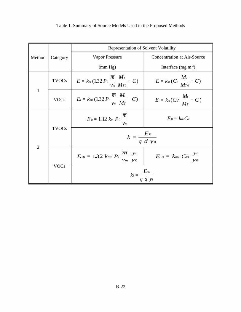
B-22
Table 1. Summary of Source Models Used in the Proposed Methods
Method Category
Representation of Solvent Volatility
Vapor Pressure
(mm Hg)
Concentration at Air-Source
Interface (mg m-3)
1
TVOCs E k Pm
v
M
MCm
m
T
T= −( . )132 0
0E k C
M
MCm v
T
T= −( )
0
VOCs E k Pm
v
M
MCi mi i
m
i
T= −( . )132 E k Cv
M
MCi m i
i
Ti= −( )
2
TVOCs
E k Pm
vm
m0 0132= . E k Cm v0 =
kE
d y=
0
0θ
VOCs
E k Pm
v
y
yi mi i
m
i0
0132= . E k C
y
yi mi vi
i0
0=
kE
d yi
i
i=
0
θ

B-23
Table 2. List of Parameters Required by the Concentration Models
Parameter SymbolMethod 1 Method 2
TVOC VOC TVOC VOC
room volume V X X X Xair exchange rate N X X X Xmass transfer coefficient km , kmi X X X Xsource area S X X X Xwet film thickness è X X X Xproduct density d X X X Xcontent of TVOC in product y0 X X X Xtotal vapor pressure for TVOC P0, Cv X X Xaverage molecular weight for TVOC m X X
content of individual VOC in product yi X X
vapor pressure for individual VOC Pi, Cvi X Xmolecular weight for individual VOC mi X
Table 3. Comparison of Headspace TVOC Concentrations with
Theoretically Calculated Cv0 for Three Wet Sources
ProductMeasured Cv0
a Computed Percent
Difference(g m-3) P0 (mm Hg) Cv0 (g m-3)
Alkyd Primer 27.2 ± 1.77 3.49 31.9 15.9 Alkyd Paint A 12.3 ± 1.66 1.44 14.3 15.0
Synthetic Stain 16.6 ± 1.91 2.86 18.4 10.3 a mean ± standard deviation; n = 6 for alkyd primer and alkyd paint; and n = 7 for synthetic stain.
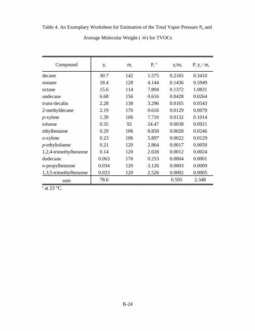
B-24
Table 4. An Exemplary Worksheet for Estimation of the Total Vapor Pressure P0 and
Average Molecular Weight ( ) for TVOCsm
Compound yi mi Pi a yi/mi Pi yi / mi
decane 30.7 142 1.575 0.2165 0.3410 nonane 18.4 128 4.144 0.1436 0.5949 octane 15.6 114 7.894 0.1372 1.0831 undecane 6.68 156 0.616 0.0428 0.0264 trans-decalin 2.28 138 3.296 0.0165 0.0543 2-methyldecane 2.19 170 0.616 0.0129 0.0079 p-xylene 1.39 106 7.710 0.0132 0.1014 toluene 0.35 92 24.47 0.0038 0.0921 ethylbenzene 0.29 106 8.850 0.0028 0.0246 o-xylene 0.23 106 5.897 0.0022 0.0129 p-ethyltoluene 0.21 120 2.864 0.0017 0.0050 1,2,4-trimethylbenzene 0.14 120 2.028 0.0012 0.0024 dodecane 0.063 170 0.253 0.0004 0.0001 n-propylbenzene 0.034 120 3.126 0.0003 0.0009 1,3,5-trimethylbenzene 0.023 120 2.526 0.0002 0.0005
sum 78.6 0.595 2.348 a at 23 °C.
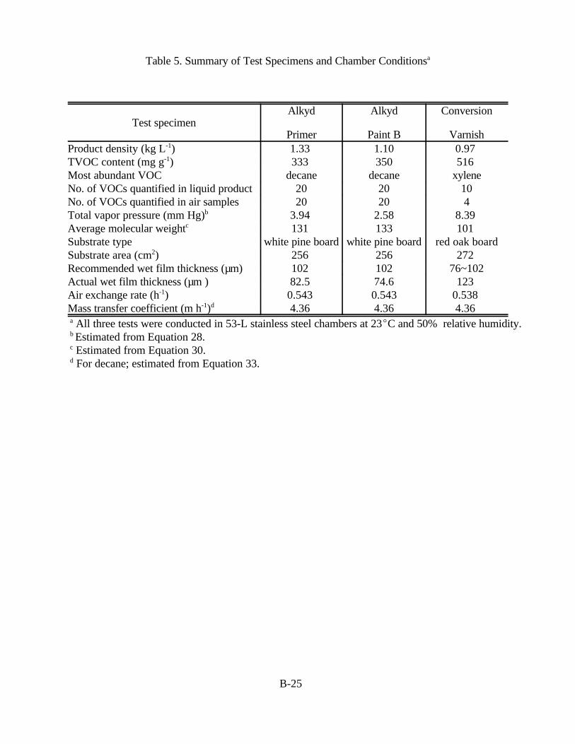
B-25
Table 5. Summary of Test Specimens and Chamber Conditionsa
Test specimenAlkyd
Primer
Alkyd
Paint B
Conversion
VarnishProduct density (kg L-1) 1.33 1.10 0.97 TVOC content (mg g-1) 333 350 516 Most abundant VOC decane decane xyleneNo. of VOCs quantified in liquid product 20 20 10No. of VOCs quantified in air samples 20 20 4Total vapor pressure (mm Hg)b 3.94 2.58 8.39 Average molecular weightc 131 133 101 Substrate type white pine board white pine board red oak boardSubstrate area (cm2) 256 256 272 Recommended wet film thickness (µm) 102 102 76~102Actual wet film thickness (µm ) 82.5 74.6 123 Air exchange rate (h-1) 0.543 0.543 0.538 Mass transfer coefficient (m h-1)d 4.36 4.36 4.36
a All three tests were conducted in 53-L stainless steel chambers at 23EC and 50% relative humidity. b Estimated from Equation 28. c Estimated from Equation 30. d For decane; estimated from Equation 33.
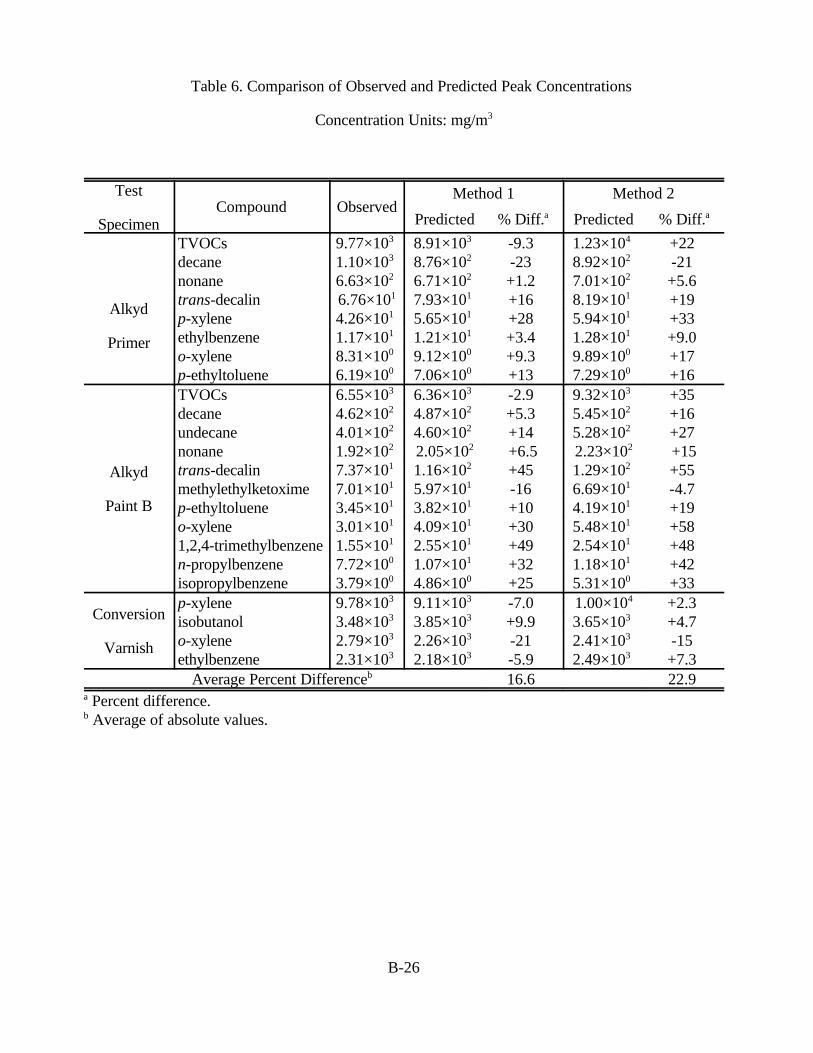
B-26
Table 6. Comparison of Observed and Predicted Peak Concentrations
Concentration Units: mg/m3
Test
SpecimenCompound Observed
Method 1 Method 2
Predicted % Diff.a Predicted % Diff.a
Alkyd
Primer
TVOCs 9.77×10³ 8.91×10³ -9.3 1.23×10⁴ +22 decane 1.10×10³ 8.76×10² -23 8.92×10² -21 nonane 6.63×10² 6.71×10² +1.2 7.01×10² +5.6 trans-decalin 6.76×101 7.93×101 +16 8.19×101 +19 p-xylene 4.26×101 5.65×101 +28 5.94×101 +33 ethylbenzene 1.17×101 1.21×101 +3.4 1.28×101 +9.0 o-xylene 8.31×100 9.12×100 +9.3 9.89×100 +17 p-ethyltoluene 6.19×100 7.06×100 +13 7.29×100 +16
Alkyd
Paint B
TVOCs 6.55×10³ 6.36×10³ -2.9 9.32×10³ +35 decane 4.62×10² 4.87×10² +5.3 5.45×10² +16 undecane 4.01×10² 4.60×10² +14 5.28×10² +27 nonane 1.92×10² 2.05×10² +6.5 2.23×10² +15 trans-decalin 7.37×101 1.16×10² +45 1.29×10² +55 methylethylketoxime 7.01×101 5.97×101 -16 6.69×101 -4.7 p-ethyltoluene 3.45×101 3.82×101 +10 4.19×101 +19 o-xylene 3.01×101 4.09×101 +30 5.48×101 +58 1,2,4-trimethylbenzene 1.55×101 2.55×101 +49 2.54×101 +48 n-propylbenzene 7.72×100 1.07×101 +32 1.18×101 +42 isopropylbenzene 3.79×100 4.86×100 +25 5.31×100 +33
Conversion
Varnish
p-xylene 9.78×10³ 9.11×10³ -7.0 1.00×10⁴ +2.3 isobutanol 3.48×10³ 3.85×10³ +9.9 3.65×10³ +4.7 o-xylene 2.79×10³ 2.26×10³ -21 2.41×10³ -15 ethylbenzene 2.31×10³ 2.18×10³ -5.9 2.49×10³ +7.3
Average Percent Differenceb 16.6 22.9 a Percent difference.b Average of absolute values.
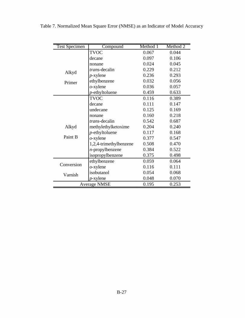
B-27
Table 7. Normalized Mean Square Error (NMSE) as an Indicator of Model Accuracy
Test Specimen Compound Method 1 Method 2
Alkyd
Primer
TVOC 0.067 0.044 decane 0.097 0.106 nonane 0.024 0.045 trans-decalin 0.229 0.212 p-xylene 0.236 0.293 ethylbenzene 0.032 0.056 o-xylene 0.036 0.057 p-ethyltoluene 0.459 0.633
Alkyd
Paint B
TVOC 0.116 0.389 decane 0.111 0.147 undecane 0.125 0.169 nonane 0.160 0.218 trans-decalin 0.542 0.687 methylethylketoxime 0.204 0.240 p-ethyltoluene 0.117 0.168 o-xylene 0.377 0.547 1,2,4-trimethylbenzene 0.508 0.470 n-propylbenzene 0.384 0.522 isopropylbenzene 0.375 0.498
Conversion
Varnish
ethylbenzene 0.059 0.064 o-xylene 0.116 0.111 isobutanol 0.054 0.068 p-xylene 0.048 0.070
Average NMSE 0.195 0.253
B-28
Figure Captions
Figure 1. Gas-phase mass transfer coefficient (km ) as a function of air velocity and source area (S)
Figure 2. An example of model predictions with good accuracy. NMSE = 0.024 for method 1 and
0.045 for method 2. Data are for nonane in the alkyd primer test.
Figure 3. An example of model predictions with poor accuracy. NMSE = 0.542 for method 1 and
0.687 for method 2. Data are for trans-decalin in the alkyd paint test.
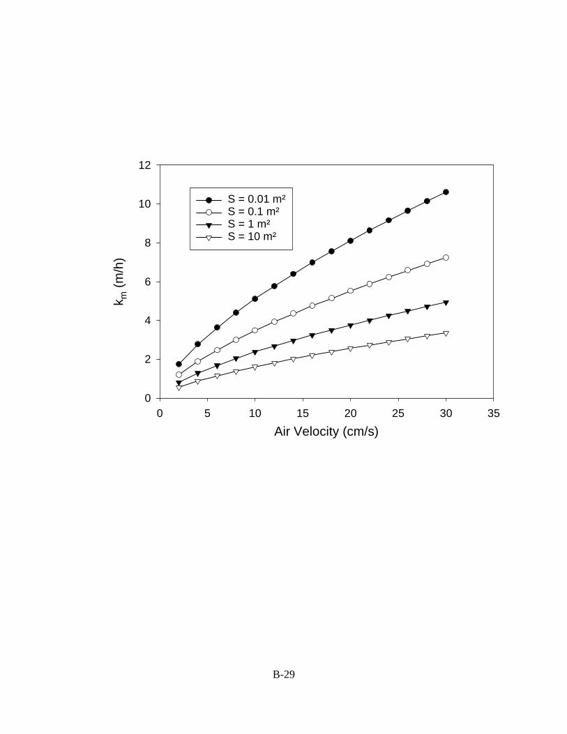
B-29
Air Velocity (cm/s)
0 5 10 15 20 25 30 35
k m (
m/h
)
0
2
4
6
8
10
12
S = 0.01 m²S = 0.1 m²S = 1 m²S = 10 m²
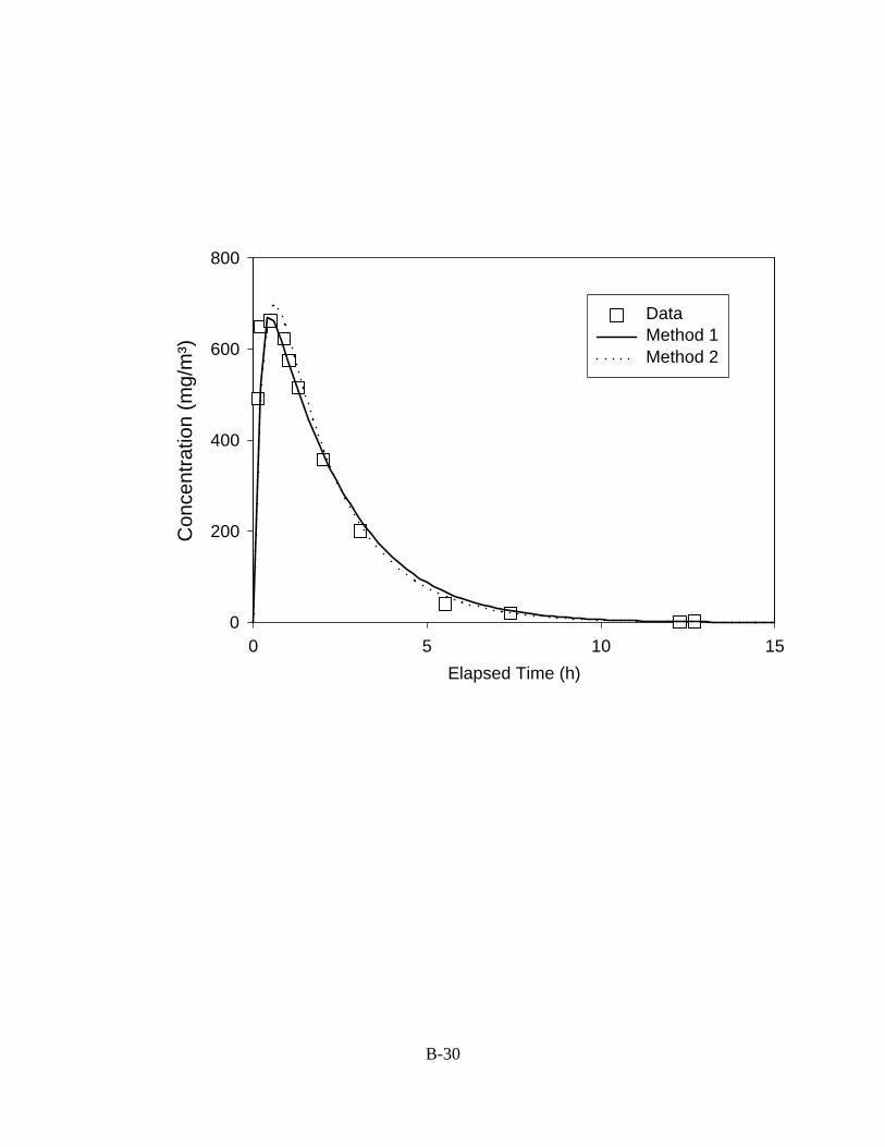
B-30
Elapsed Time (h)
0 5 10 15
Con
cent
ratio
n (m
g/m
³)
0
200
400
600
800
DataMethod 1Method 2
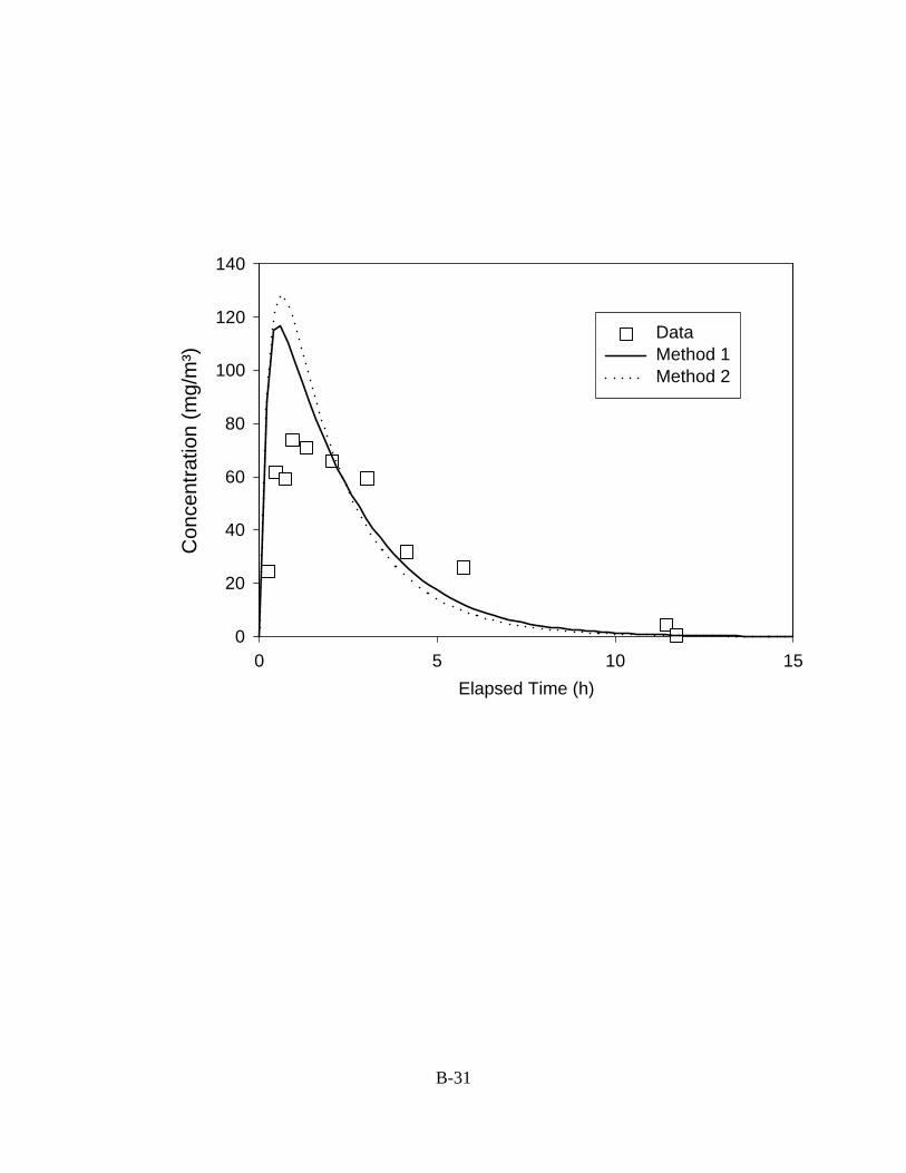
B-31
Elapsed Time (h)
0 5 10 15
Con
cent
ratio
n (m
g/m
³)
0
20
40
60
80
100
120
140
DataMethod 1Method 2
APPENDIX C
LATEX PAINT CHAMBER TESTS

C-1
C1. INTRODUCTION
A series of small-chamber tests was conducted by ARCADIS Geraghty and Miller, Inc., to
characterize concentrations of various volatile organic compounds (VOCs) emitted from different
formulations of latex primer and paint. In addition to the broad objective of improving the
understanding of emission behavior for these chemicals in latex primer and paint, a more specific
objective was to provide a quantitative basis for development of emission models or for estimating
parameters for such models. In addition to the small-chamber tests, ARCADIS Geraghty and
Miller, Inc., conducted painting events at EPA’s research house in North Carolina for the primary
purpose of gathering data to be used for model evaluation.
The sections that follow describe methods and results for bulk analysis of the latex
primer/paint formulations prior to chamber testing, small-chamber emission tests of these
formulations, and development of predictive models for VOC emissions from latex primer and
paint.
C2. BULK ANALYSIS
Prior to conduct of small-chamber emission tests, each formulation of latex primer or paint
was analyzed to determine its chemical composition by weight. In brief, the procedure for
analysis of the bulk product that was followed by ARCADIS Geraghty and Miller, Inc.,
(ARCADIS 1998) involved (1) extracting latex primer and paints with acetone, (2) centrifuging
the sample to remove solids, and (3) analyzing the supernatant by GC/MS. Aliquots of the
supernatant were diluted as necessary to yield sample concentrations that fell within the
calibration range.
Results of the bulk analysis are shown as chemical weight fractions (mg/g) in Table C-1.
One primer (designated as formulation LP-A) was used for the chamber tests together with four
formulations of paint (LF-B, LF-C, LSG-D, and LSG-E). In the designations for formulation, P
indicates primer, F indicates flat paint, and SG indicates semi-gloss paint. Only five VOCs were
found in measurable quantities in any of the formulations that were tested. The primer contained
ethylene glycol and TMPD-MIB, the flat paints primarily contained propylene glycol and TMPD-
MIB, and the semi-gloss paints primarily contained propylene glycol and TMPD-MIB. Thus,
TMPD-MIB was the only VOC common to all formulations. One semi-gloss formulation had a
measurable, but relatively small, quantity of 2-(2-butoxyethoxy) ethanol (BEE), and one of the
flat paints and one of the semi-gloss paints had relatively small quantities of dipropylene glycol.
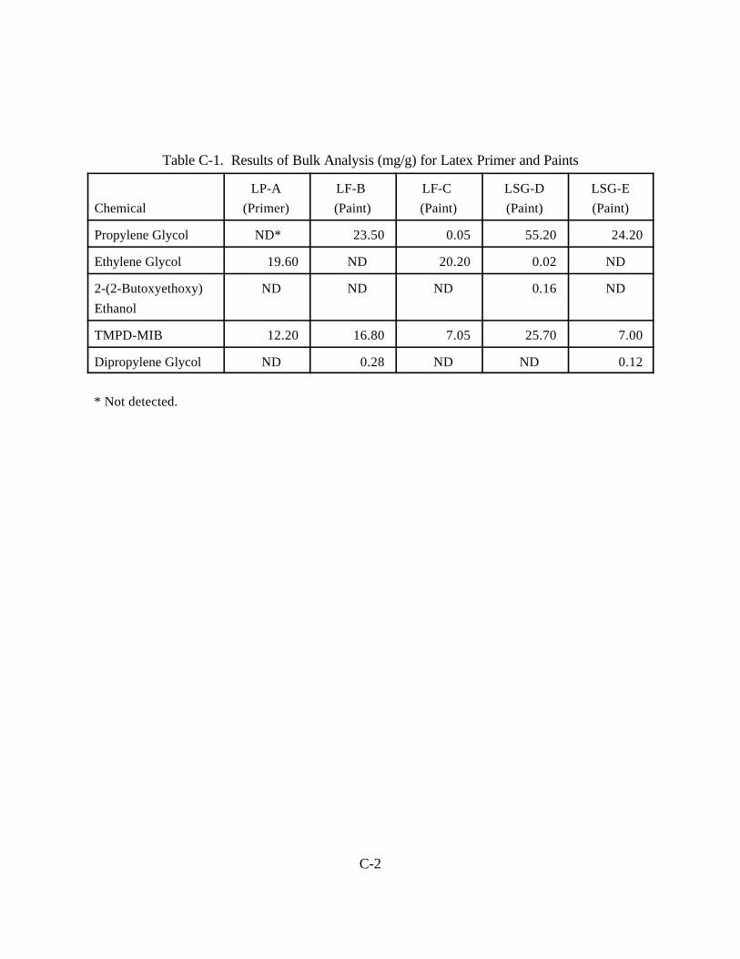
C-2
Table C-1. Results of Bulk Analysis (mg/g) for Latex Primer and Paints
Chemical
LP-A
(Primer)
LF-B
(Paint)
LF-C
(Paint)
LSG-D
(Paint)
LSG-E
(Paint)
Propylene Glycol ND* 23.50 0.05 55.20 24.20
Ethylene Glycol 19.60 ND 20.20 0.02 ND
2-(2-Butoxyethoxy)
Ethanol
ND ND ND 0.16 ND
TMPD-MIB 12.20 16.80 7.05 25.70 7.00
Dipropylene Glycol ND 0.28 ND ND 0.12
* Not detected.
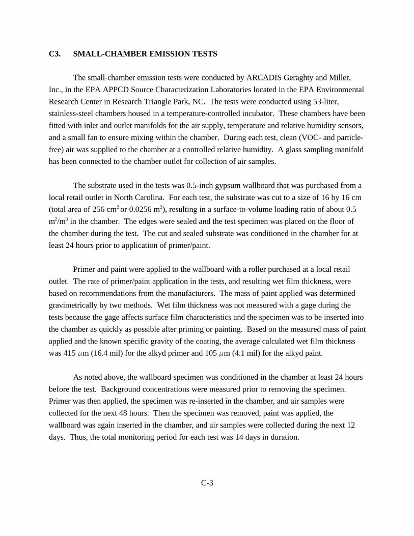
C-3
C3. SMALL-CHAMBER EMISSION TESTS
The small-chamber emission tests were conducted by ARCADIS Geraghty and Miller,
Inc., in the EPA APPCD Source Characterization Laboratories located in the EPA Environmental
Research Center in Research Triangle Park, NC. The tests were conducted using 53-liter,
stainless-steel chambers housed in a temperature-controlled incubator. These chambers have been
fitted with inlet and outlet manifolds for the air supply, temperature and relative humidity sensors,
and a small fan to ensure mixing within the chamber. During each test, clean (VOC- and particle-
free) air was supplied to the chamber at a controlled relative humidity. A glass sampling manifold
has been connected to the chamber outlet for collection of air samples.
The substrate used in the tests was 0.5-inch gypsum wallboard that was purchased from a
local retail outlet in North Carolina. For each test, the substrate was cut to a size of 16 by 16 cm
(total area of 256 cm2 or 0.0256 m2), resulting in a surface-to-volume loading ratio of about 0.5
m2/m3 in the chamber. The edges were sealed and the test specimen was placed on the floor of
the chamber during the test. The cut and sealed substrate was conditioned in the chamber for at
least 24 hours prior to application of primer/paint.
Primer and paint were applied to the wallboard with a roller purchased at a local retail
outlet. The rate of primer/paint application in the tests, and resulting wet film thickness, were
based on recommendations from the manufacturers. The mass of paint applied was determined
gravimetrically by two methods. Wet film thickness was not measured with a gage during the
tests because the gage affects surface film characteristics and the specimen was to be inserted into
the chamber as quickly as possible after priming or painting. Based on the measured mass of paint
applied and the known specific gravity of the coating, the average calculated wet film thickness
was 415 Fm (16.4 mil) for the alkyd primer and 105 Fm (4.1 mil) for the alkyd paint.
As noted above, the wallboard specimen was conditioned in the chamber at least 24 hours
before the test. Background concentrations were measured prior to removing the specimen.
Primer was then applied, the specimen was re-inserted in the chamber, and air samples were
collected for the next 48 hours. Then the specimen was removed, paint was applied, the
wallboard was again inserted in the chamber, and air samples were collected during the next 12
days. Thus, the total monitoring period for each test was 14 days in duration.
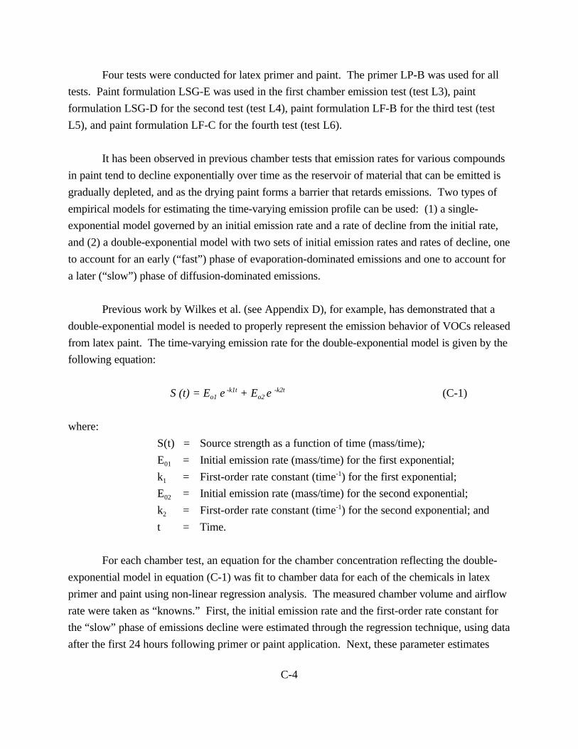
C-4
Four tests were conducted for latex primer and paint. The primer LP-B was used for all
tests. Paint formulation LSG-E was used in the first chamber emission test (test L3), paint
formulation LSG-D for the second test (test L4), paint formulation LF-B for the third test (test
L5), and paint formulation LF-C for the fourth test (test L6).
It has been observed in previous chamber tests that emission rates for various compounds
in paint tend to decline exponentially over time as the reservoir of material that can be emitted is
gradually depleted, and as the drying paint forms a barrier that retards emissions. Two types of
empirical models for estimating the time-varying emission profile can be used: (1) a single-
exponential model governed by an initial emission rate and a rate of decline from the initial rate,
and (2) a double-exponential model with two sets of initial emission rates and rates of decline, one
to account for an early (“fast”) phase of evaporation-dominated emissions and one to account for
a later (“slow”) phase of diffusion-dominated emissions.
Previous work by Wilkes et al. (see Appendix D), for example, has demonstrated that a
double-exponential model is needed to properly represent the emission behavior of VOCs released
from latex paint. The time-varying emission rate for the double-exponential model is given by the
following equation:
S (t) = Eo1 e -k1t + Eo2 e -k2t (C-1)
where:
S(t) = Source strength as a function of time (mass/time);
E01 = Initial emission rate (mass/time) for the first exponential;
k1 = First-order rate constant (time-1) for the first exponential;
E02 = Initial emission rate (mass/time) for the second exponential;
k2 = First-order rate constant (time-1) for the second exponential; and
t = Time.
For each chamber test, an equation for the chamber concentration reflecting the double-
exponential model in equation (C-1) was fit to chamber data for each of the chemicals in latex
primer and paint using non-linear regression analysis. The measured chamber volume and airflow
rate were taken as “knowns.” First, the initial emission rate and the first-order rate constant for
the “slow” phase of emissions decline were estimated through the regression technique, using data
after the first 24 hours following primer or paint application. Next, these parameter estimates
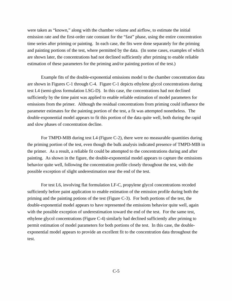
C-5
were taken as “known,” along with the chamber volume and airflow, to estimate the initial
emission rate and the first-order rate constant for the “fast” phase, using the entire concentration
time series after priming or painting. In each case, the fits were done separately for the priming
and painting portions of the test, where permitted by the data. (In some cases, examples of which
are shown later, the concentrations had not declined sufficiently after priming to enable reliable
estimation of these parameters for the priming and/or painting portion of the test.)
Example fits of the double-exponential emissions model to the chamber concentration data
are shown in Figures C-1 through C-4. Figure C-1 depicts ethylene glycol concentrations during
test L4 (semi-gloss formulation LSG-D). In this case, the concentrations had not declined
sufficiently by the time paint was applied to enable reliable estimation of model parameters for
emissions from the primer. Although the residual concentrations from priming could influence the
parameter estimates for the painting portion of the test, a fit was attempted nonetheless. The
double-exponential model appears to fit this portion of the data quite well, both during the rapid
and slow phases of concentration decline.
For TMPD-MIB during test L4 (Figure C-2), there were no measurable quantities during
the priming portion of the test, even though the bulk analysis indicated presence of TMPD-MIB in
the primer. As a result, a reliable fit could be attempted to the concentrations during and after
painting. As shown in the figure, the double-exponential model appears to capture the emissions
behavior quite well, following the concentration profile closely throughout the test, with the
possible exception of slight underestimation near the end of the test.
For test L6, involving flat formulation LF-C, propylene glycol concentrations receded
sufficiently before paint application to enable estimation of the emission profile during both the
priming and the painting potions of the test (Figure C-3). For both portions of the test, the
double-exponential model appears to have represented the emissions behavior quite well, again
with the possible exception of underestimation toward the end of the test. For the same test,
ethylene glycol concentrations (Figure C-4) similarly had declined sufficiently after priming to
permit estimation of model parameters for both portions of the test. In this case, the double-
exponential model appears to provide an excellent fit to the concentration data throughout the
test.
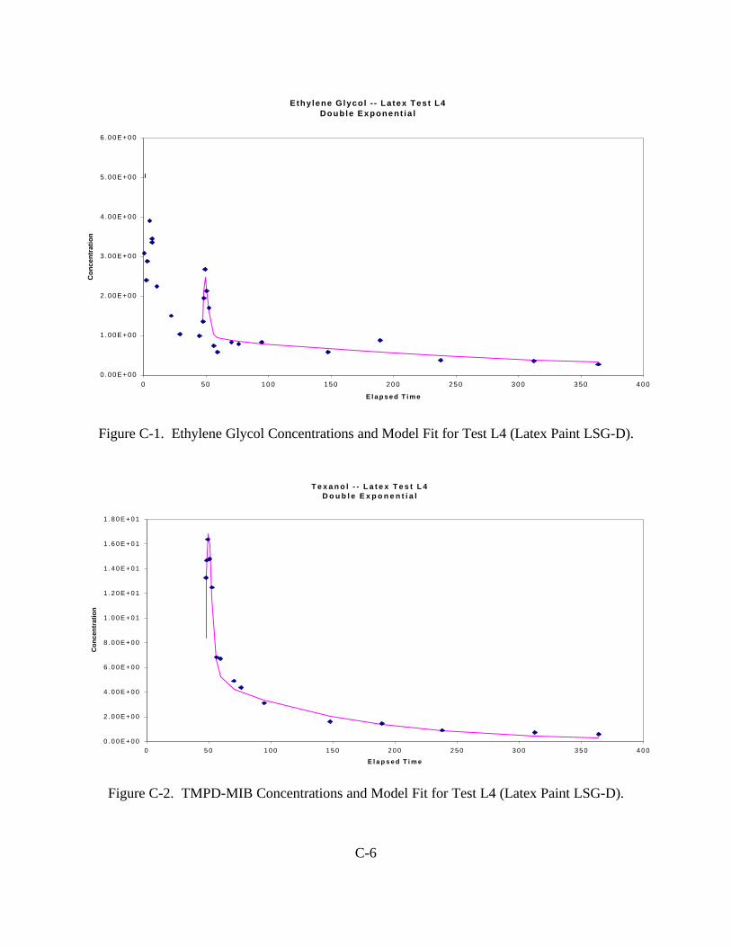
C-6
Ethylene Glycol - - Latex Test L4Double Exponent ia l
0 .00E+00
1 .00E+00
2 .00E+00
3 .00E+00
4 .00E+00
5 .00E+00
6 .00E+00
0 50 100 150 200 250 300 350 400
E l a p s e d T i m e
Co
nce
ntr
atio
n
T e x a n o l - - L a t e x T e s t L 4D o u b l e E x p o n e n t i a l
0 . 0 0 E + 0 0
2 . 0 0 E + 0 0
4 . 0 0 E + 0 0
6 . 0 0 E + 0 0
8 . 0 0 E + 0 0
1 . 0 0 E + 0 1
1 . 2 0 E + 0 1
1 . 4 0 E + 0 1
1 . 6 0 E + 0 1
1 . 8 0 E + 0 1
0 5 0 1 0 0 1 5 0 2 0 0 2 5 0 3 0 0 3 5 0 4 0 0
E l a p s e d T i m e
Co
nce
ntr
atio
n
Figure C-1. Ethylene Glycol Concentrations and Model Fit for Test L4 (Latex Paint LSG-D).
Figure C-2. TMPD-MIB Concentrations and Model Fit for Test L4 (Latex Paint LSG-D).
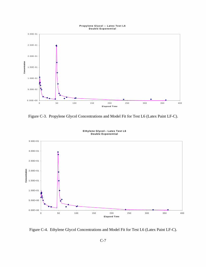
C-7
P r o p y l e n e G l y c o l - - L a t e x T e s t L 6D o u b l e E x p o n e n t i a l
0 . 0 0 E + 0 0
5 . 0 0 E - 0 2
1 . 0 0 E - 0 1
1 . 5 0 E - 0 1
2 . 0 0 E - 0 1
2 . 5 0 E - 0 1
3 . 0 0 E - 0 1
0 5 0 1 0 0 1 5 0 2 0 0 2 5 0 3 0 0 3 5 0 4 0 0
E l a p s e d T i m e
Co
nce
ntr
atio
n
Ethylene Glycol-- Latex Test L6Double Exponential
0.00E+00
5.00E+00
1.00E+01
1.50E+01
2.00E+01
2.50E+01
3.00E+01
3.50E+01
0 50 100 150 200 250 300 350 400
Elapsed Time
Co
nce
ntr
atio
n
Figure C-3. Propylene Glycol Concentrations and Model Fit for Test L6 (Latex Paint LF-C).
Figure C-4. Ethylene Glycol Concentrations and Model Fit for Test L6 (Latex Paint LF-C).
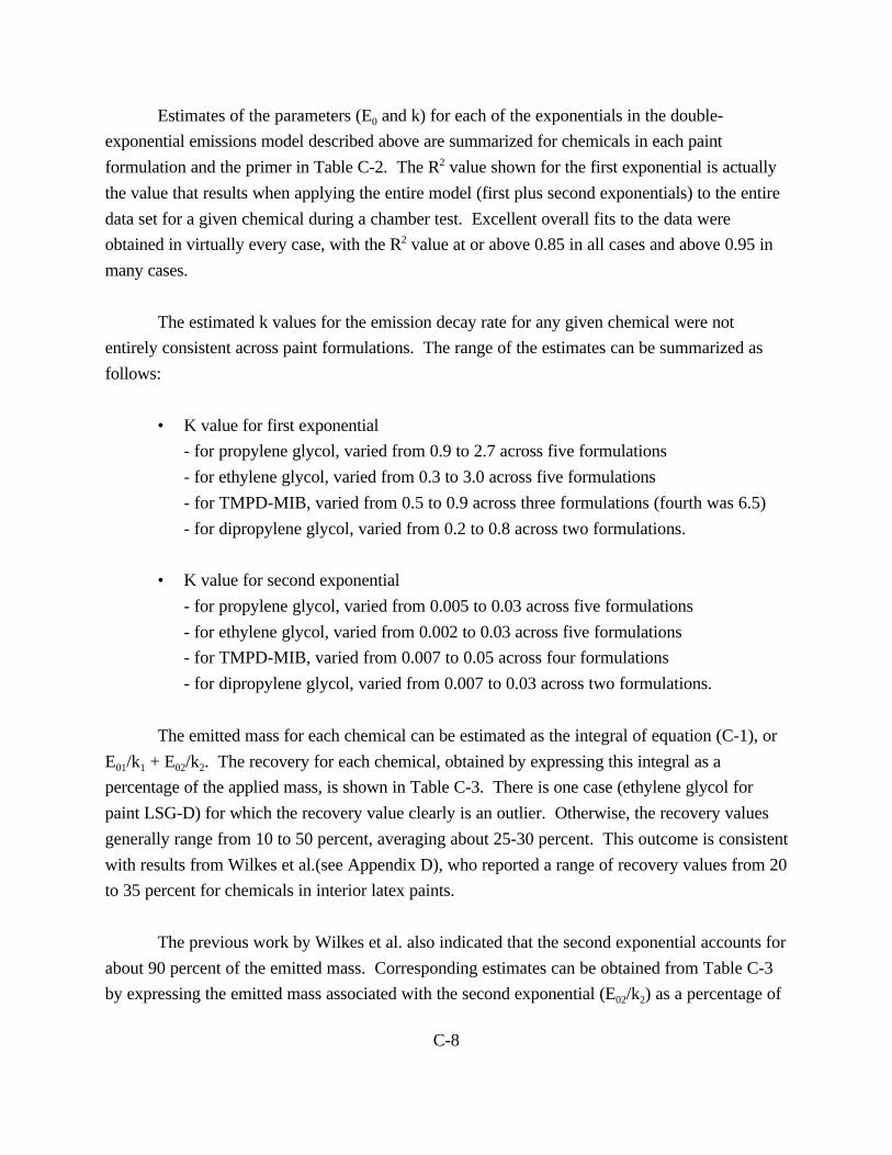
C-8
Estimates of the parameters (E0 and k) for each of the exponentials in the double-
exponential emissions model described above are summarized for chemicals in each paint
formulation and the primer in Table C-2. The R2 value shown for the first exponential is actually
the value that results when applying the entire model (first plus second exponentials) to the entire
data set for a given chemical during a chamber test. Excellent overall fits to the data were
obtained in virtually every case, with the R2 value at or above 0.85 in all cases and above 0.95 in
many cases.
The estimated k values for the emission decay rate for any given chemical were not
entirely consistent across paint formulations. The range of the estimates can be summarized as
follows:
• K value for first exponential
- for propylene glycol, varied from 0.9 to 2.7 across five formulations
- for ethylene glycol, varied from 0.3 to 3.0 across five formulations
- for TMPD-MIB, varied from 0.5 to 0.9 across three formulations (fourth was 6.5)
- for dipropylene glycol, varied from 0.2 to 0.8 across two formulations.
• K value for second exponential
- for propylene glycol, varied from 0.005 to 0.03 across five formulations
- for ethylene glycol, varied from 0.002 to 0.03 across five formulations
- for TMPD-MIB, varied from 0.007 to 0.05 across four formulations
- for dipropylene glycol, varied from 0.007 to 0.03 across two formulations.
The emitted mass for each chemical can be estimated as the integral of equation (C-1), or
E01/k1 + E02/k2. The recovery for each chemical, obtained by expressing this integral as a
percentage of the applied mass, is shown in Table C-3. There is one case (ethylene glycol for
paint LSG-D) for which the recovery value clearly is an outlier. Otherwise, the recovery values
generally range from 10 to 50 percent, averaging about 25-30 percent. This outcome is consistent
with results from Wilkes et al.(see Appendix D), who reported a range of recovery values from 20
to 35 percent for chemicals in interior latex paints.
The previous work by Wilkes et al. also indicated that the second exponential accounts for
about 90 percent of the emitted mass. Corresponding estimates can be obtained from Table C-3
by expressing the emitted mass associated with the second exponential (E02/k2) as a percentage of
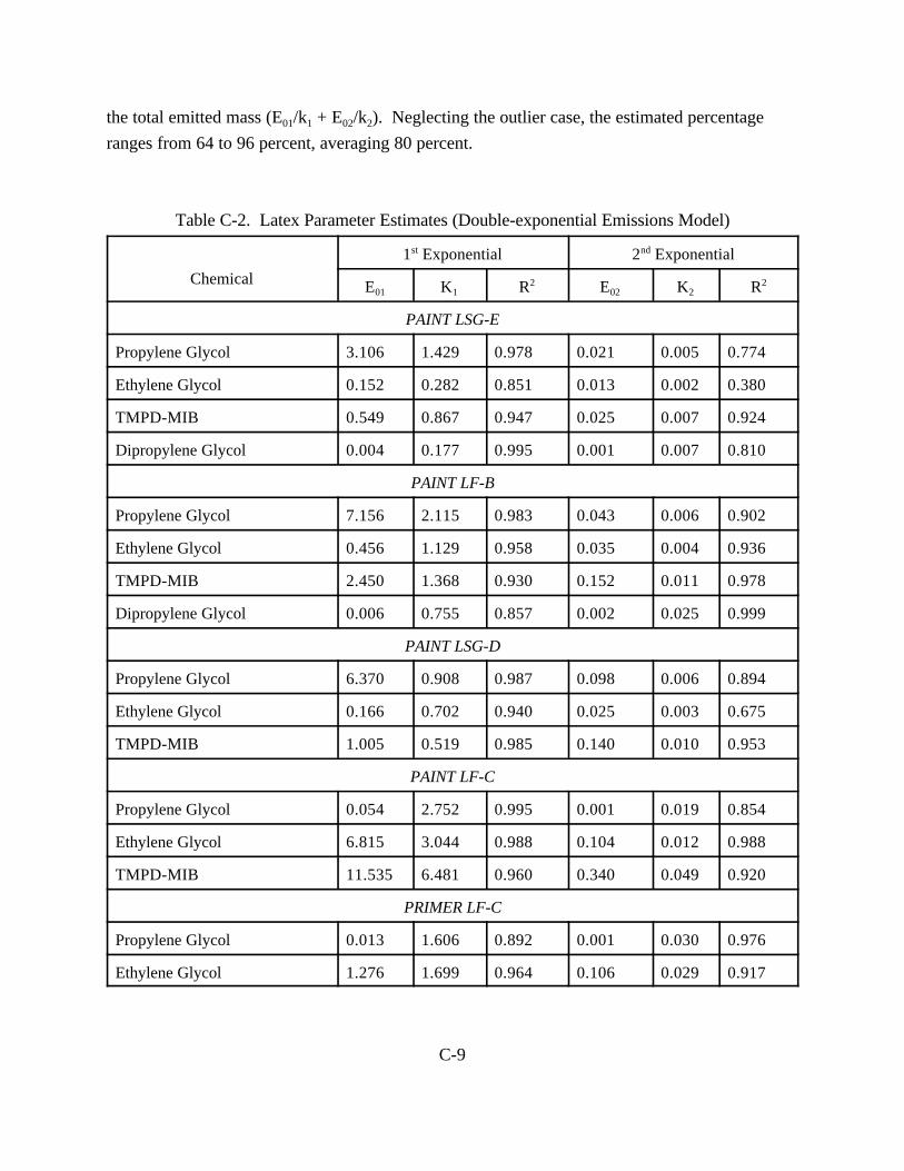
C-9
the total emitted mass (E01/k1 + E02/k2). Neglecting the outlier case, the estimated percentage
ranges from 64 to 96 percent, averaging 80 percent.
Table C-2. Latex Parameter Estimates (Double-exponential Emissions Model)
Chemical
1st Exponential 2nd Exponential
E01 K1 R2 E02 K2 R2
PAINT LSG-E
Propylene Glycol 3.106 1.429 0.978 0.021 0.005 0.774
Ethylene Glycol 0.152 0.282 0.851 0.013 0.002 0.380
TMPD-MIB 0.549 0.867 0.947 0.025 0.007 0.924
Dipropylene Glycol 0.004 0.177 0.995 0.001 0.007 0.810
PAINT LF-B
Propylene Glycol 7.156 2.115 0.983 0.043 0.006 0.902
Ethylene Glycol 0.456 1.129 0.958 0.035 0.004 0.936
TMPD-MIB 2.450 1.368 0.930 0.152 0.011 0.978
Dipropylene Glycol 0.006 0.755 0.857 0.002 0.025 0.999
PAINT LSG-D
Propylene Glycol 6.370 0.908 0.987 0.098 0.006 0.894
Ethylene Glycol 0.166 0.702 0.940 0.025 0.003 0.675
TMPD-MIB 1.005 0.519 0.985 0.140 0.010 0.953
PAINT LF-C
Propylene Glycol 0.054 2.752 0.995 0.001 0.019 0.854
Ethylene Glycol 6.815 3.044 0.988 0.104 0.012 0.988
TMPD-MIB 11.535 6.481 0.960 0.340 0.049 0.920
PRIMER LF-C
Propylene Glycol 0.013 1.606 0.892 0.001 0.030 0.976
Ethylene Glycol 1.276 1.699 0.964 0.106 0.029 0.917
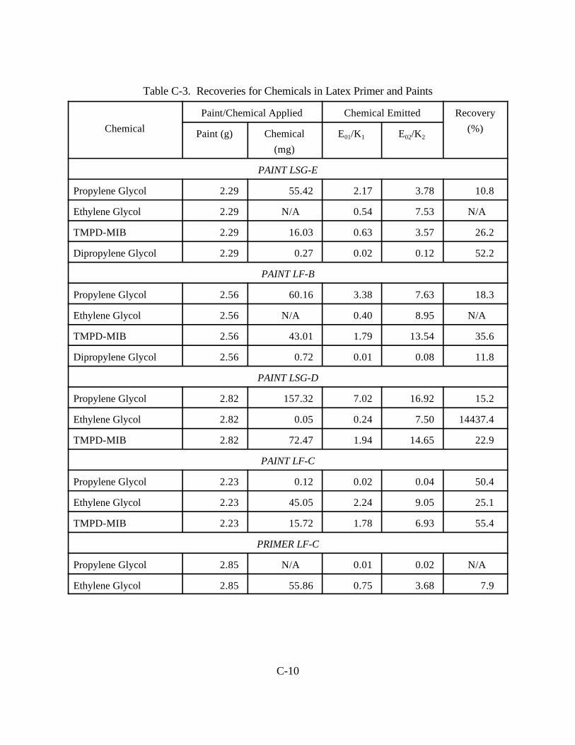
C-10
Table C-3. Recoveries for Chemicals in Latex Primer and Paints
Chemical
Paint/Chemical Applied Chemical Emitted Recovery
(%)Paint (g) Chemical
(mg)
E01/K1 E02/K2
PAINT LSG-E
Propylene Glycol 2.29 55.42 2.17 3.78 10.8
Ethylene Glycol 2.29 N/A 0.54 7.53 N/A
TMPD-MIB 2.29 16.03 0.63 3.57 26.2
Dipropylene Glycol 2.29 0.27 0.02 0.12 52.2
PAINT LF-B
Propylene Glycol 2.56 60.16 3.38 7.63 18.3
Ethylene Glycol 2.56 N/A 0.40 8.95 N/A
TMPD-MIB 2.56 43.01 1.79 13.54 35.6
Dipropylene Glycol 2.56 0.72 0.01 0.08 11.8
PAINT LSG-D
Propylene Glycol 2.82 157.32 7.02 16.92 15.2
Ethylene Glycol 2.82 0.05 0.24 7.50 14437.4
TMPD-MIB 2.82 72.47 1.94 14.65 22.9
PAINT LF-C
Propylene Glycol 2.23 0.12 0.02 0.04 50.4
Ethylene Glycol 2.23 45.05 2.24 9.05 25.1
TMPD-MIB 2.23 15.72 1.78 6.93 55.4
PRIMER LF-C
Propylene Glycol 2.85 N/A 0.01 0.02 N/A
Ethylene Glycol 2.85 55.86 0.75 3.68 7.9
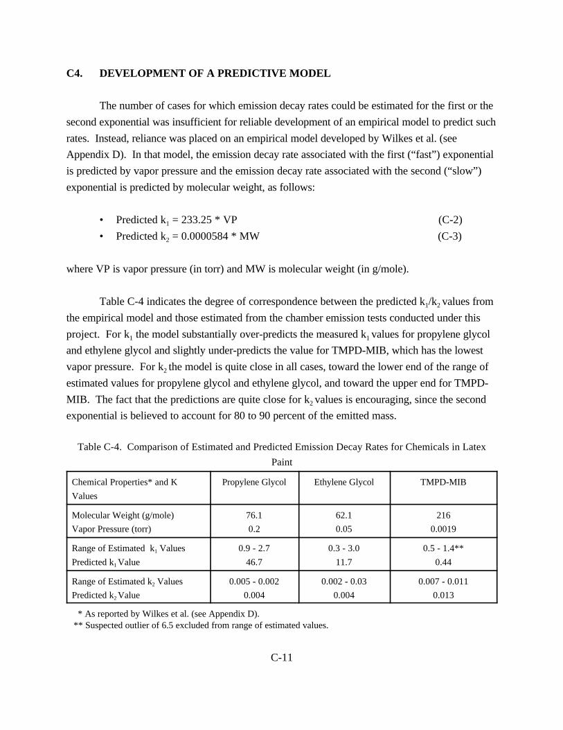
C-11
C4. DEVELOPMENT OF A PREDICTIVE MODEL
The number of cases for which emission decay rates could be estimated for the first or the
second exponential was insufficient for reliable development of an empirical model to predict such
rates. Instead, reliance was placed on an empirical model developed by Wilkes et al. (see
Appendix D). In that model, the emission decay rate associated with the first (“fast”) exponential
is predicted by vapor pressure and the emission decay rate associated with the second (“slow”)
exponential is predicted by molecular weight, as follows:
• Predicted k1 = 233.25 * VP (C-2)
• Predicted k2 = 0.0000584 * MW (C-3)
where VP is vapor pressure (in torr) and MW is molecular weight (in g/mole).
Table C-4 indicates the degree of correspondence between the predicted k1/k2 values from
the empirical model and those estimated from the chamber emission tests conducted under this
project. For k1 the model substantially over-predicts the measured k1 values for propylene glycol
and ethylene glycol and slightly under-predicts the value for TMPD-MIB, which has the lowest
vapor pressure. For k2 the model is quite close in all cases, toward the lower end of the range of
estimated values for propylene glycol and ethylene glycol, and toward the upper end for TMPD-
MIB. The fact that the predictions are quite close for k2 values is encouraging, since the second
exponential is believed to account for 80 to 90 percent of the emitted mass.
Table C-4. Comparison of Estimated and Predicted Emission Decay Rates for Chemicals in Latex
Paint
Chemical Properties* and K
Values
Propylene Glycol Ethylene Glycol TMPD-MIB
Molecular Weight (g/mole)
Vapor Pressure (torr)
76.1
0.2
62.1
0.05
216
0.0019
Range of Estimated k1 Values
Predicted k1 Value
0.9 - 2.7
46.7
0.3 - 3.0
11.7
0.5 - 1.4**
0.44
Range of Estimated k2 Values
Predicted k2 Value
0.005 - 0.002
0.004
0.002 - 0.03
0.004
0.007 - 0.011
0.013
* As reported by Wilkes et al. (see Appendix D). ** Suspected outlier of 6.5 excluded from range of estimated values.
APPENDIX D
PAPER ON EMISSIONS MODEL FOR LATEX PAINT(presented at Indoor Air ‘96 Conference)
D-1
ESTIMATION OF EMISSION PROFILESFOR INTERIOR LATEX PAINTS
C.Wilkes1, M.Koontz1, M.Ryan2 and C.Cinalli2
1GEOMET Technologies, Inc., Germantown, MD, USA2Office of Pollution Prevention and Toxics, US Environmental Protection Agency, Washington DC, USA
ABSTRACT
Methods were developed for estimating emission profiles for VOCs released from interior latexpaints, for two situations: time-series data are available from small-chamber experiments; andonly the weight fractions and physical/chemical properties of the paint constituents are known. A double-exponential model fit the data quite well in most cases. The rate constant for the“fast” (evaporation-dominated) exponential is related to vapor pressure, and the rate constantfor the “slow” (diffusion-dominated) exponential is related to molecular weight. Although thefast component dominates the early phase of the emission profile, it generally accounts for 10percent or less of the released VOC mass. The mass released, in turn, generally was between20 and 35 percent of the applied VOC mass.
INTRODUCTION
Estimation of human inhalation exposure in residential settings, due to use of consumerproducts or installation of building materials or furnishings, requires integration of time-varyingpollutant concentrations with information on individuals’ locations and breathing rates. Oftenthe concentration component is estimated using an indoor air quality (IAQ) model. Theaccuracy of the exposure estimate is enhanced by providing a faithful depiction of the time-varying airborne concentration which, in turn, relies on reasonable characterization of theemission profile for the chemical(s) of concern.
The main objective of the effort described in this paper was to develop methods for estimatingemission profiles for chemicals released from interior latex paints, for two situations: data areavailable from small-chamber experiments whereby airborne concentrations are measured inthe chamber at selected points in time after the paint has been instantaneously applied to asubstrate; and only the weight fractions and physical/chemical properties (molecular weightand vapor pressure) of the paint constituents are known. Small-chamber data used for thisanalysis have been recently collected for latex paint applied to gypsum board (1).
METHODS
The experimental data were collected under sponsorship of the EPA Air and EnergyEngineering Research Laboratory (AEERL) in Research Triangle Park, NC. Theseexperiments involved application of two different formulations, called A and B in this paper, oflatex paint to a small piece of pre-painted gypsum board. Following the paint application,
D-2
the specimen was immediately inserted in a small stainless-steel chamber, and concentrations offour individual VOCs were measured at selected points in time over a period of severalhundred hours. Multiple samples were collected during each experiment on TenaxTA sorbentand analyzed by a gas chromatograph with a flame ionization detector (GC/FID). The sampledurations were variable, ranging from an hour or less at the start of the experiment to muchlonger durations toward the end, when the chamber air concentrations were lower.
Bulk analysis of the paint sample was performed to determine which volatile organiccompounds (VOCs) are present in each paint, and to estimate the weight fraction of eachVOC. Four individual VOCs were found to comprise the majority of the VOCs present ineach paint. The molecular weight (MW) and vapor pressure (VP) of these four compoundswere estimated (2) to be:
• Propylene Glycol: MW = 76.1 g/mol VP = 0.2 torr• Ethylene Glycol: MW = 62.1 g/mol VP = 0.05 torr• Butoxyethoxyethanol: MW = 162.2 g/mol VP = 0.02 torr• Texanol: MW = 216 g/mol VP = 0.0019 torr
Various representations of the emission profile were considered, including a mass-transferrepresentation based on physical and chemical properties, an empirically fit single-exponentialmodel to account for the (assumed) general decline in the emission rate over time, and anempirically fit double-exponential model (the sum of two exponentials) that assumes twocomponents of emissions decline -- a “fast” (evaporation-dominated) component that primarilygoverns the early stage of emissions and a “slow” (diffusion-dominated) component thatgoverns the later stage. The exponential model is given by the following equation:
S(t) =E0 e-kt (1)
where: S(t) = Source strength as a function of time (mass/time)E0
= Initial emission rate (mass/time)k = First-order rate constant (time-1)t = Time.
For estimation of the single- and double-exponential model parameters (an initial emission rateand a first-order rate of decline in the rate), nonlinear regression analysis was applied to thechamber concentration data, taking advantage of the known chamber volume and theexperimentally controlled air exchange rate for the chamber.
RESULTS
The mass-transfer model was found by other researchers (1) to provide a good fit to measuredair concentrations. However, because of the large number of parameters that are difficult toestimate or must be measured, it was not possible to use this model for this study. Based onthe results of the nonlinear estimation process, the single-exponential model did not fit the datawell, most likely because it is insufficient to provide an empirical representation of the physicalprocess as the paint dries. The double-exponential model fit the data quite well in most cases.
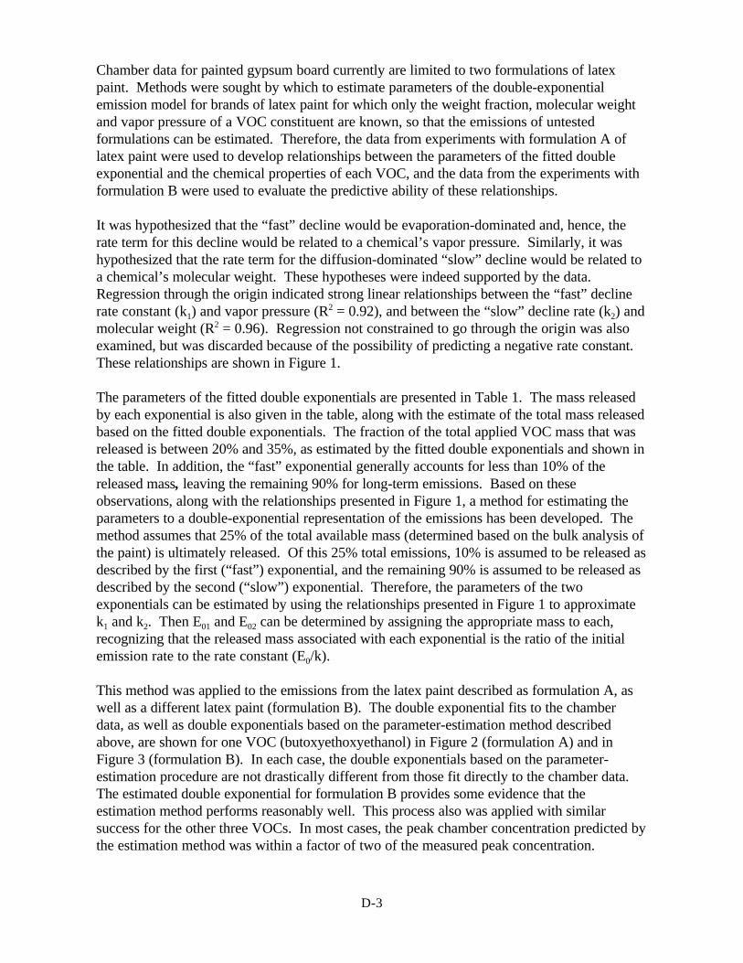
D-3
Chamber data for painted gypsum board currently are limited to two formulations of latexpaint. Methods were sought by which to estimate parameters of the double-exponentialemission model for brands of latex paint for which only the weight fraction, molecular weightand vapor pressure of a VOC constituent are known, so that the emissions of untestedformulations can be estimated. Therefore, the data from experiments with formulation A oflatex paint were used to develop relationships between the parameters of the fitted doubleexponential and the chemical properties of each VOC, and the data from the experiments withformulation B were used to evaluate the predictive ability of these relationships.
It was hypothesized that the “fast” decline would be evaporation-dominated and, hence, therate term for this decline would be related to a chemical’s vapor pressure. Similarly, it washypothesized that the rate term for the diffusion-dominated “slow” decline would be related toa chemical’s molecular weight. These hypotheses were indeed supported by the data. Regression through the origin indicated strong linear relationships between the “fast” declinerate constant (k1) and vapor pressure (R2 = 0.92), and between the “slow” decline rate (k2) andmolecular weight (R2 = 0.96). Regression not constrained to go through the origin was alsoexamined, but was discarded because of the possibility of predicting a negative rate constant. These relationships are shown in Figure 1.
The parameters of the fitted double exponentials are presented in Table 1. The mass releasedby each exponential is also given in the table, along with the estimate of the total mass releasedbased on the fitted double exponentials. The fraction of the total applied VOC mass that wasreleased is between 20% and 35%, as estimated by the fitted double exponentials and shown inthe table. In addition, the “fast” exponential generally accounts for less than 10% of thereleased mass, leaving the remaining 90% for long-term emissions. Based on theseobservations, along with the relationships presented in Figure 1, a method for estimating theparameters to a double-exponential representation of the emissions has been developed. Themethod assumes that 25% of the total available mass (determined based on the bulk analysis ofthe paint) is ultimately released. Of this 25% total emissions, 10% is assumed to be released asdescribed by the first (“fast”) exponential, and the remaining 90% is assumed to be released asdescribed by the second (“slow”) exponential. Therefore, the parameters of the twoexponentials can be estimated by using the relationships presented in Figure 1 to approximatek1 and k2. Then E01 and E02 can be determined by assigning the appropriate mass to each,recognizing that the released mass associated with each exponential is the ratio of the initialemission rate to the rate constant (E0/k).
This method was applied to the emissions from the latex paint described as formulation A, aswell as a different latex paint (formulation B). The double exponential fits to the chamberdata, as well as double exponentials based on the parameter-estimation method describedabove, are shown for one VOC (butoxyethoxyethanol) in Figure 2 (formulation A) and inFigure 3 (formulation B). In each case, the double exponentials based on the parameter-estimation procedure are not drastically different from those fit directly to the chamber data. The estimated double exponential for formulation B provides some evidence that theestimation method performs reasonably well. This process also was applied with similar success for the other three VOCs. In most cases, the peak chamber concentration predicted bythe estimation method was within a factor of two of the measured peak concentration.
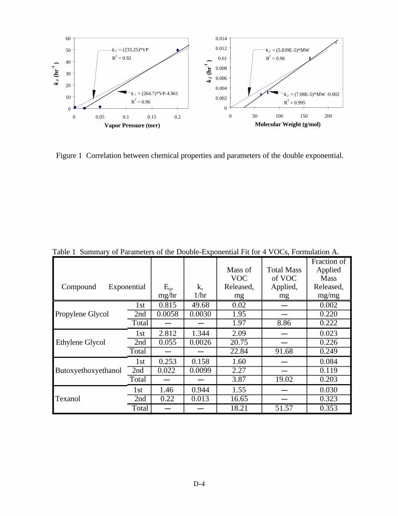
D-4
Figure 1 Correlation between chemical properties and parameters of the double exponential.
0
10
20
30
40
50
60
0 0.05 0.1 0.15 0.2
Vapor Pressure (torr)
k1
(hr-1
)
k 1 = (264.7)*VP-4.961
R2 = 0.96
k 1 = (233.25)*VP
R2 = 0.92
0
0.002
0.004
0.006
0.008
0.01
0.012
0.014
0 50 100 150 200
Molecular Weight (g/mol)
k2
(hr-1
)
k 2 = (7.08E-5)*MW -0.002
R2 = 0.995
k 2 = (5.839E-5)*MW
R2 = 0.96
Table 1 Summary of Parameters of the Double-Exponential Fit for 4 VOCs, Formulation A.
Compound Exponential E0, k,
Mass ofVOC
Released,
Total Massof VOCApplied,
Fraction ofApplied
MassReleased,
mg/hr 1/hr mg mg mg/mg1st 0.815 49.68 0.02 --- 0.002
Propylene Glycol 2nd 0.0058 0.0030 1.95 --- 0.220Total --- --- 1.97 8.86 0.2221st 2.812 1.344 2.09 --- 0.023
Ethylene Glycol 2nd 0.055 0.0026 20.75 --- 0.226Total --- --- 22.84 91.68 0.249
1st 0.253 0.158 1.60 --- 0.084Butoxyethoxyethanol 2nd 0.022 0.0099 2.27 --- 0.119
Total --- --- 3.87 19.02 0.2031st 1.46 0.944 1.55 --- 0.030
Texanol 2nd 0.22 0.013 16.65 --- 0.323Total --- --- 18.21 51.57 0.353
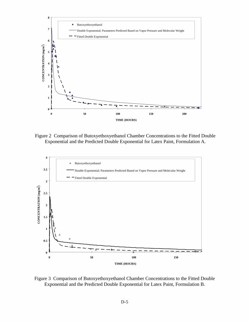
D-5
0
1
2
3
4
5
6
7
8
0 50 100 150 200
TIME (HOURS)
CO
NC
EN
TR
AT
ION
(m
g/m
3 )
Butoxyethoxyethanol
Double Exponential; Parameters Predicted Based on Vapor Pressure and Molecular Weight
Fitted Double Exponential
0
0.5
1
1.5
2
2.5
3
3.5
4
0 50 100 150
TIME (HOURS)
CO
NC
EN
TR
AT
ION
(m
g/m
3 )
Butoxyethoxyethanol
Double Exponential; Parameters Predicted Based on Vapor Pressure and Molecular Weight
Fitted Double Exponential
Figure 2 Comparison of Butoxyethoxyethanol Chamber Concentrations to the Fitted DoubleExponential and the Predicted Double Exponential for Latex Paint, Formulation A.
Figure 3 Comparison of Butoxyethoxyethanol Chamber Concentrations to the Fitted DoubleExponential and the Predicted Double Exponential for Latex Paint, Formulation B.
D-6
CONCLUSIONS
The double-exponential model was found to fit the data quite well in most cases, provided thatthe second (“slow”) exponential was estimated first, by fitting a single-exponential model tothe data after the first 48 hours in the chamber. The first (“fast”) exponential could then beestimated using all the chamber data, by specifying a double-exponential model with the secondexponential’s parameters input as “knowns.”
Integration of the fitted double-exponential model to infinity provided an estimate of the totalemitted mass of each VOC. Comparison of this emitted mass with the applied mass, asestimated from the bulk analysis, indicated that the emitted mass ranged from 20 to 35 percentof the applied mass for those compounds, averaging about 25 percent. Integration of therespective exponentials indicated that the amount of emitted mass attributable to the first(“fast”) exponential was generally less than 10 percent. Thus, although this exponentialdominates the early emission phase, the later phase of “slow” emissions accounts for most ofthe total VOC emissions.
A relationship between the parameters of the double exponential and the chemical properties ofthe VOC was identified. Because the VOCs are leaving the paint primarily throughevaporation in the initial phases of the paint-drying process, it is reasonable for the rateconstant to be correlated with the VOC’s vapor pressure. Similarly, the VOCs are leavinglater in the paint-drying process primarily through diffusion, and in this case it is reasonable forthe rate constant to the be correlated with the VOC’s molecular weight. The number of datapoints is small, and therefore these relationships cannot be used with great confidence,especially for VOCs with vapor pressures and molecular weights outside the range of thoseexamined in this study. With data from additional chamber tests, the confidence in theserelationships could be improved, and a physically/chemically based mass-transfer model couldbe developed.
Several areas where improved information or theoretical developments would aid any futureiterations of estimation procedures for interior latex paints are apparent. More small-chamberexperimental data for paint applied to gypsum board are needed so that differences across flat,semi-gloss and gloss paints can be evaluated, and so that a broader array of individual VOCs isavailable to support development of regression estimates. Ideally, a physically and chemicallybased model could be developed that accounts for the mass-transfer process yet requires onlyminimum parameter estimates such as VOC weight faction, vapor pressure and molecularweight, with possible addition of selected parameters specific to the painting event (e.g., paintapplication rate, indoor volume).
ACKNOWLEDGMENTS
This work was funded by the US Environmental Protection Agency under contract number68-D3-0013.

D-7
REFERENCES
(1) Acurex Environmental Corporation. 1995. “Data Summary for the Latex PaintAssessment Program. II. Dynamic and Static Chamber Testing and ModelDevelopment”, Report Prepared for the US Environmental Protection Agency UnderContract Number 68-D4-0005, June 9, 1995.
(2) Environmental Fate Database, Syracuse Research Corporation, Syracuse, NY, USA.
APPENDIX E
MODEL EVALUATION USING DATA FROM EPA RESEARCH HOUSE
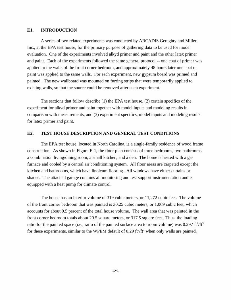
E-1
E1. INTRODUCTION
A series of two related experiments was conducted by ARCADIS Geraghty and Miller,
Inc., at the EPA test house, for the primary purpose of gathering data to be used for model
evaluation. One of the experiments involved alkyd primer and paint and the other latex primer
and paint. Each of the experiments followed the same general protocol -- one coat of primer was
applied to the walls of the front corner bedroom, and approximately 48 hours later one coat of
paint was applied to the same walls. For each experiment, new gypsum board was primed and
painted. The new wallboard was mounted on furring strips that were temporarily applied to
existing walls, so that the source could be removed after each experiment.
The sections that follow describe (1) the EPA test house, (2) certain specifics of the
experiment for alkyd primer and paint together with model inputs and modeling results in
comparison with measurements, and (3) experiment specifics, model inputs and modeling results
for latex primer and paint.
E2. TEST HOUSE DESCRIPTION AND GENERAL TEST CONDITIONS
The EPA test house, located in North Carolina, is a single-family residence of wood frame
construction. As shown in Figure E-1, the floor plan consists of three bedrooms, two bathrooms,
a combination living/dining room, a small kitchen, and a den. The home is heated with a gas
furnace and cooled by a central air conditioning system. All floor areas are carpeted except the
kitchen and bathrooms, which have linoleum flooring. All windows have either curtains or
shades. The attached garage contains all monitoring and test support instrumentation and is
equipped with a heat pump for climate control.
The house has an interior volume of 319 cubic meters, or 11,272 cubic feet. The volume
of the front corner bedroom that was painted is 30.25 cubic meters, or 1,069 cubic feet, which
accounts for about 9.5 percent of the total house volume. The wall area that was painted in the
front corner bedroom totals about 29.5 square meters, or 317.5 square feet. Thus, the loading
ratio for the painted space (i.e., ratio of the painted surface area to room volume) was 0.297 ft2/ft3
for these experiments, similar to the WPEM default of 0.29 ft2/ft3 when only walls are painted.
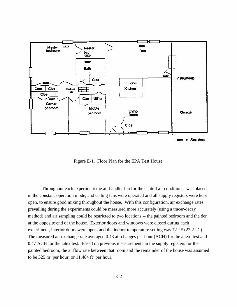
E-2
Figure E-1. Floor Plan for the EPA Test House.
Throughout each experiment the air handler fan for the central air conditioner was placed
in the constant-operation mode, and ceiling fans were operated and all supply registers were kept
open, to ensure good mixing throughout the house. With this configuration, air exchange rates
prevailing during the experiments could be measured more accurately (using a tracer-decay
method) and air sampling could be restricted to two locations -- the painted bedroom and the den
at the opposite end of the house. Exterior doors and windows were closed during each
experiment, interior doors were open, and the indoor temperature setting was 72 EF (22.2 EC).
The measured air exchange rate averaged 0.48 air changes per hour (ACH) for the alkyd test and
0.47 ACH for the latex test. Based on previous measurements in the supply registers for the
painted bedroom, the airflow rate between that room and the remainder of the house was assumed
to be 325 m3 per hour, or 11,484 ft3 per hour.
E-3
Background air samples were collected both outdoors and in the house prior to each of
the two experiments. Paint was applied approximately 48 hours after primer application, and air
samples were collected over a 14-day period (48 hours after priming and 12 days after painting),
at a progressively lower rate as indoor concentrations receded following the priming/painting
event. The latex test was conducted first (August 1997). Following the 14-day measurement
period, the painted wallboard was removed, the house was aired out, and then new wallboard was
installed for the alkyd test (September 1997).
E3. MODEL EVALUATION FOR ALKYD PRIMER AND PAINT
The report of the experiments by ARCADIS Geraghty and Miller, Inc., indicates that,
for the alkyd experiment, 6.96 kilograms of primer AP-F were applied to the walls in the front
corner bedroom over a period of 43.4 minutes, beginning at 11:13 a.m. on September 9, 1997.
Approximately two days later, 4.93 kilograms of paint ASG-G were applied over a period of 33.7
minutes, beginning at 10:41 a.m. on September 11, 1997. The reported wet film thickness was
14.4 mil for primer and 8.05 mil for paint. The measured air exchange rate prevailing during the
test averaged 0.48 ACH, as noted previously.
Corresponding WPEM inputs for the painting scenario described above are summarized in
Table E-1. The input for house volume matched the actual value listed above. The percent
painted was set to 9.5 percent, resulting in a painted volume of 1071 ft3 (the actual painted
volume was 1069 ft3). The inputs for air exchange and interzonal airflow rates matched the actual
values listed above. Based on a loading ratio of 0.30 ft2/ft3 for walls, the painted surface area
input was 321 ft2 (the actual area was 317.5 ft2).
The wet film thickness values reported by ARCADIS Geraghty and Miller, Inc. -- 6 mil
for primer and 5.375 mil for paint -- correspond to primer/paint coverages of 267 and 298
ft2/gallon, respectively. The application rates input for WPEM -- 1.66 gallons/hour for primer and
1.92 gallons/hour for paint -- were chosen to result in priming/painting durations that matched
those reported for the experiment at the EPA test house.
E-4
Table E-1. WPEM Inputs for Alkyd Painting Scenario at EPA Test House
Input Parameter Input Value
House volume 11,272 ft3
Percent of house painted 9.5 %
Air exchange rate 0.48 ACH
Interzonal airflow rate 11,484 ft3/hour
Painted wall surface area 321 ft2 (using loading ratio of 0.30; actual = 317.5 ft2)
Wet film thickness 6 mil for primer, 5.375 mil for paint
Calculated amount of paint 1.20 gallons for primer, 1.08 gallons for paint
Application rate 1.66 gallons/hour for primer, 1.92 gallons/hour for paint
Calculated application time 0.72 hours for primer, 0.56 hours for paint
Primer/paint interval Paint second day after priming
WPEM inputs pertaining specifically to the modeled paint and chemical are listed in Table
E-2. The paint density values were chosen such that the product of gallons applied times paint
density yielded the applied-mass values reported by ARCADIS Geraghty and Miller, Inc. -- 6.96
kg for primer and 4.93 kg for paint. The first chemical modeled was undecane, one of the primary
constituents by weight in both alkyd primer and paint, with physical/chemical properties as listed
in the table. The input values for weight fraction were based on the results of bulk analysis for
primer and paint (see Appendix A, Section A2). The default emission decay rate calculated by the
empirical emissions model in WPEM was used; the basis for the WPEM algorithm to calculate
this default value is described in Appendix A, Section A4. Based on results of sink tests
conducted by ARCADIS Geraghty and Miller, Inc. (see Appendix A, Section A5), indoor sinks
were assumed to be negligible.
A DIY painter was arbitrarily chosen as the exposed individual. WPEM inputs for
occupancy and exposure affect exposure/dose calculations, but the interest here was in a
comparison of modeled versus measured indoor concentrations (there were no exposure/dose
measurements). The model was run for 4 days with a 5-minute reporting interval.
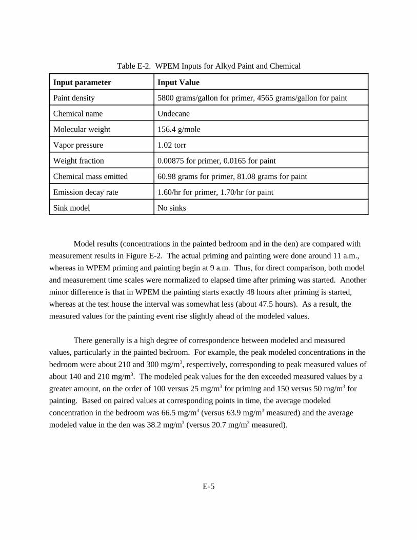
E-5
Table E-2. WPEM Inputs for Alkyd Paint and Chemical
Input parameter Input Value
Paint density 5800 grams/gallon for primer, 4565 grams/gallon for paint
Chemical name Undecane
Molecular weight 156.4 g/mole
Vapor pressure 1.02 torr
Weight fraction 0.00875 for primer, 0.0165 for paint
Chemical mass emitted 60.98 grams for primer, 81.08 grams for paint
Emission decay rate 1.60/hr for primer, 1.70/hr for paint
Sink model No sinks
Model results (concentrations in the painted bedroom and in the den) are compared with
measurement results in Figure E-2. The actual priming and painting were done around 11 a.m.,
whereas in WPEM priming and painting begin at 9 a.m. Thus, for direct comparison, both model
and measurement time scales were normalized to elapsed time after priming was started. Another
minor difference is that in WPEM the painting starts exactly 48 hours after priming is started,
whereas at the test house the interval was somewhat less (about 47.5 hours). As a result, the
measured values for the painting event rise slightly ahead of the modeled values.
There generally is a high degree of correspondence between modeled and measured
values, particularly in the painted bedroom. For example, the peak modeled concentrations in the
bedroom were about 210 and 300 mg/m3, respectively, corresponding to peak measured values of
about 140 and 210 mg/m3. The modeled peak values for the den exceeded measured values by a
greater amount, on the order of 100 versus 25 mg/m3 for priming and 150 versus 50 mg/m3 for
painting. Based on paired values at corresponding points in time, the average modeled
concentration in the bedroom was 66.5 mg/m3 (versus 63.9 mg/m3 measured) and the average
modeled value in the den was 38.2 mg/m3 (versus 20.7 mg/m3 measured).
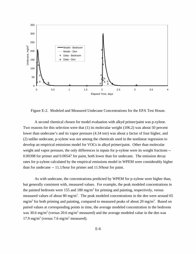
E-6
0
50
100
150
200
250
300
350
0 0.5 1 1.5 2 2.5 3 3.5 4
Elapsed Time, days
Und
ecan
e, m
g/m
3
Model - Bedroom
Model - Den
Data - Bedroom
Data - Den
Figure E-2. Modeled and Measured Undecane Concentrations for the EPA Test House.
A second chemical chosen for model evaluation with alkyd primer/paint was p-xylene.
Two reasons for this selection were that (1) its molecular weight (106.2) was about 50 percent
lower than undecane’s and its vapor pressure (4.34 torr) was about a factor of four higher, and
(2) unlike undecane, p-xylene was not among the chemicals used in the nonlinear regression to
develop an empirical emissions model for VOCs in alkyd primer/paint. Other than molecular
weight and vapor pressure, the only differences in inputs for p-xylene were its weight fractions --
0.00398 for primer and 0.00547 for paint, both lower than for undecane. The emission decay
rates for p-xylene calculated by the empirical emissions model in WPEM were considerably higher
than for undecane -- 11.1/hour for primer and 11.9/hour for paint.
As with undecane, the concentrations predicted by WPEM for p-xylene were higher than,
but generally consistent with, measured values. For example, the peak modeled concentrations in
the painted bedroom were 155 and 180 mg/m3 for priming and painting, respectively, versus
measured values of about 80 mg/m3. The peak modeled concentrations in the den were around 65
mg/m3 for both priming and painting, compared to measured peaks of about 20 mg/m3. Based on
paired values at corresponding points in time, the average modeled concentration in the bedroom
was 30.6 mg/m3 (versus 20.6 mg/m3 measured) and the average modeled value in the den was
17.9 mg/m3 (versus 7.6 mg/m3 measured).
E-7
E3. MODEL EVALUATION FOR LATEX PRIMER AND PAINT
The report of the experiments by ARCADIS Geraghty and Miller, Inc., indicates that,
for the latex experiment, 5.26 kilograms of primer LP-A were applied to the walls in the front
corner bedroom over a period of 36.4 minutes, beginning at 11:18 a.m. on August 20, 1997.
Approximately two days later, 4.65 kilograms of paint LSG-E were applied over a period of 35.4
minutes, beginning at 10:02 a.m. on August 22, 1997. The reported wet film thickness was 7.72
mil for primer and 5.17 mil for paint. The measured air exchange rate prevailing during the test
averaged 0.47 ACH.
Corresponding WPEM inputs for the painting scenario described above are summarized in
Table E-3. Inputs for house volume, percent painted, interzonal airflow rate and painted surface
area were the same as for the alkyd test.
The wet film thickness values reported by ARCADIS Geraghty and Miller, Inc. -- 6.88 mil
for primer and 5.17 mil for paint -- correspond to primer/paint coverage rates of 233 and 310
ft2/gallon, respectively. The input painting rates of 2.27 gallons per hour for primer and 1.76
gallons per hour for paint are higher than typical values that have been reported for do-it-yourself
painters (on the order of 0.5 to 1 gallon/hour), but were were chosen to result in priming/painting
durations that matched those reported for the experiment at the EPA test house.
Table E-3. WPEM Inputs for Latex Painting Scenario at EPA Test House
Input Parameter Input Value
House volume 11,272 ft3
Percent of house painted 9.5 %
Air exchange rate 0.47 ACH
Interzonal airflow rate 11,484 ft3/hour
Painted wall surface area 321 ft2 (using loading ratio of 0.30; actual = 317.5 ft2)
Wet film thickness 6.882 mil for primer, 5.171 mil for paint
Calculated amount of paint 1.38 gallons for primer, 1.04 gallons for paint
Application rate 2.27 gallons/hour for primer, 1.76 gallons/hour for paint
Calculated application time 0.61 hours for primer, 0.59 hours for paint
Primer/paint interval Paint second day after priming
E-8
WPEM inputs pertaining specifically to the paint and chemical are listed in Table E-4. The
paint density values were chosen such that the product of gallons applied times paint density
yielded the applied-mass values reported by ARCADIS Geraghty and Miller, Inc. -- 5.26 kg for
primer and 4.65 kg for paint. The first chemical modeled was TMPD-MIB, one of the primary
constituents by weight in both latex primer and paint, with physical/chemical properties as listed in
the table. The input values for weight fraction were based on the results of bulk analysis for
primer and paint (see Appendix C, Section C2). The default emission decay rate calculated by the
empirical emissions model in WPEM was used; the basis for the WPEM algorithm to calculate
this default value is described in Appendix C (Section C4). Indoor sinks were assumed to be
negligible.
Table E-4. WPEM Inputs for Latex Paint and Chemical
Input parameter Input Value
Paint density 3812 grams/gallon for primer, 4471 grams/gallon for paint
Chemical name TMPD-MIB
Molecular weight 216 g/mole
Vapor pressure 0.0019 torr
Weight fraction 0.0122 for primer, 0.007 for paint
Chemical mass emitted* 16.02 grams for primer, 8.10 grams for paint
Emission decay rate
- first exponential
- second exponential
0.44/hr for primer and paint
0.01/hr for primer and paint
Sink model No sinks
*For the empirical emissions model for latex primer/paint, 25 % of the applied chemical mass
is assumed to be emitted.
A DIY painter was arbitrarily chosen as the exposed individual. WPEM inputs for
occupancy and exposure affect exposure/dose calculations, but the interest here was in a
comparison modeled versus measured indoor concentrations (there were no exposure/dose
measurements). The model was run for 7 days with a 5-minute reporting interval.
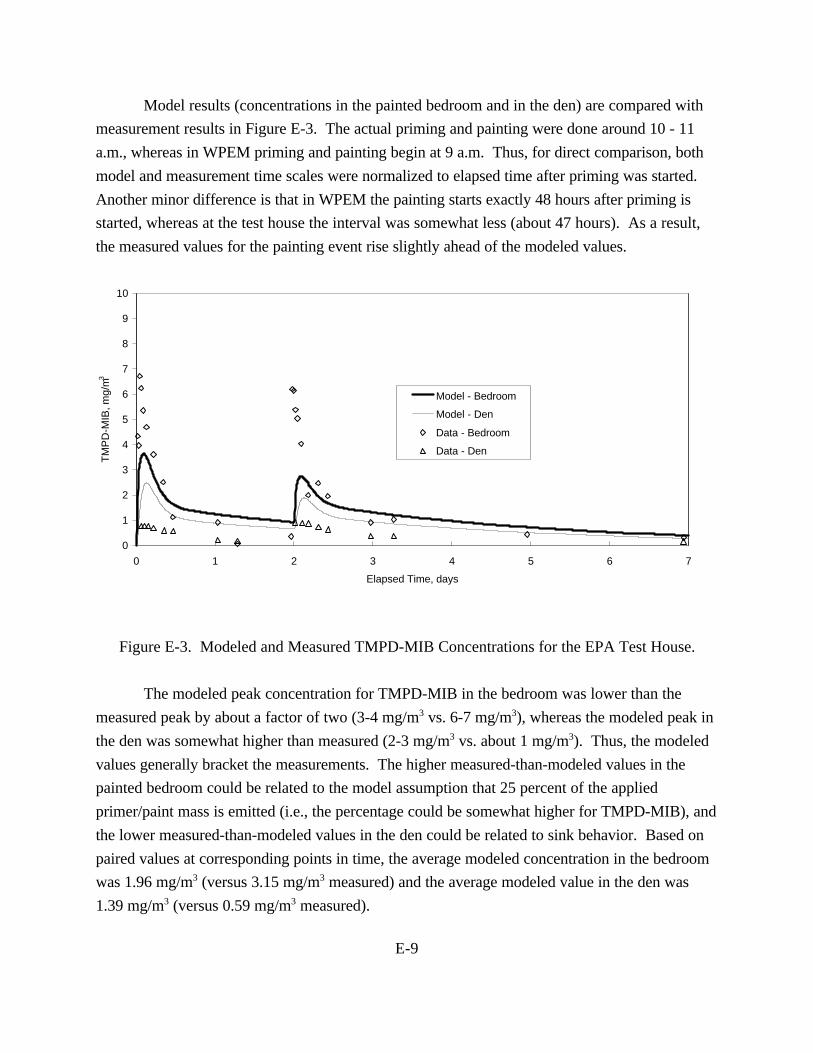
E-9
0
1
2
3
4
5
6
7
8
9
10
0 1 2 3 4 5 6 7
Elapsed Time, days
TM
PD
-MIB
, mg/
m3
Model - Bedroom
Model - Den
Data - Bedroom
Data - Den
Model results (concentrations in the painted bedroom and in the den) are compared with
measurement results in Figure E-3. The actual priming and painting were done around 10 - 11
a.m., whereas in WPEM priming and painting begin at 9 a.m. Thus, for direct comparison, both
model and measurement time scales were normalized to elapsed time after priming was started.
Another minor difference is that in WPEM the painting starts exactly 48 hours after priming is
started, whereas at the test house the interval was somewhat less (about 47 hours). As a result,
the measured values for the painting event rise slightly ahead of the modeled values.
Figure E-3. Modeled and Measured TMPD-MIB Concentrations for the EPA Test House.
The modeled peak concentration for TMPD-MIB in the bedroom was lower than the
measured peak by about a factor of two (3-4 mg/m3 vs. 6-7 mg/m3), whereas the modeled peak in
the den was somewhat higher than measured (2-3 mg/m3 vs. about 1 mg/m3). Thus, the modeled
values generally bracket the measurements. The higher measured-than-modeled values in the
painted bedroom could be related to the model assumption that 25 percent of the applied
primer/paint mass is emitted (i.e., the percentage could be somewhat higher for TMPD-MIB), and
the lower measured-than-modeled values in the den could be related to sink behavior. Based on
paired values at corresponding points in time, the average modeled concentration in the bedroom
was 1.96 mg/m3 (versus 3.15 mg/m3 measured) and the average modeled value in the den was
1.39 mg/m3 (versus 0.59 mg/m3 measured).
E-10
The second chemical modeled was propylene glycol. The bulk analysis indicated that this
chemical was not detected in primer and had a weight fraction of 0.0242 in the paint. The value
entered for the primer weight fraction in WPEM was 0.000001, the lowest value allowed. The
modeled peak concentrations in the bedroom and den were about 19 and 7 mg/m3, as compared
with measured values of 8 and 1 mg/m3. The relatively high modeled peaks are driven primarily
by the emission rate decay constant for the first exponential of the empirical (double-exponential)
emissions model.
As noted in Appendix C (see Table C-4), the predicted rate value for the decay constant of
the first exponential for propylene glycol (46.7/hour) was considerably higher than values
estimated from small-chamber emission tests (range from 0.9 to 2.7/hour). With a rate constant
of 1.8/hour, the modeled peak concentrations dropped to about 11 mg/m3 in the bedroom and 5
mg/m3 in the den. With this rate constant, the average modeled concentration in the bedroom was
1.37 mg/m3 (versus 1.41 mg/m3 measured) and the average modeled value in the den was 0.74
mg/m3 (versus 0.20 mg/m3 measured).