Working Paper No. 01-03-02

Cointegration and Threshold Adjustment

Walter Enders and Pierre Silkos

Forthcoming Journal of Business and Economic Statistics

September 2000

Cointegration and Threshold Adjustment*

Walter EndersDepartment of Economics, Finance and Legal Studies

University of AlabamaTuscaloosa, AL

35487and

Pierre L. SiklosDepartment of EconomicsWilfrid Laurier University

andClarica Financial Services Research Centre

Waterloo, OntarioCANADA N2L 3C5

ABSTRACTThis paper proposes an extension to the Engle-Granger testing strategy by permitting asymmetry inthe adjustment toward equilibrium in two different ways. We demonstrate that our test has goodpower and size properties over the Engle-Granger test when there are asymmetric departures fromequilibrium. We consider an application, namely whether there exists cointegration among interestrates for instruments with different maturities. This issue has been widely tested with mixedresults. We argue that either cautious policy, or possibly opportunistic behavior on the part of theFed, implies that an equilibrium relationship between short and long-term interest rates exists butthat adjustments from disequilibrium are asymmetric in nature. Empirical tests using US yieldsconfirm the asymmetric nature of error correction among interest rates of different maturities.

JEL Classifications: E43, C22, C50Keywords: Asymmetric Adjustment, Monte Carlo, Nonlinear Autoregression

* Research for this paper was largely conducted while both authors were Visiting Scholars at theUniversity of California, San Diego. Both authors are grateful to the Economics Department atUCSD for their hospitality and to Nathan Balke, Graham Elliott, Rob Engle, Judith Giles, theEditor and an Associate Editor, for comments and helpful discussions. Earlier versions werepresented at the EC Conference, the Third International Conference in Financial Economics in2

Juneau, Alaska, the Econometric Society Meetings, Aarhus University, the Banco de Portugal,Claremont McKenna College, the Canadian, New Zealand, and Midwest Econometric StudyGroups.

1

1. Introduction

One important development in the recent time-series literature is the examination of non-linear

adjustment mechanisms. Much of the impetus for this interest stems from a large number of studies

showing that key macroeconomic variables such as real GDP, unemployment, and industrial production

display asymmetric adjustment over the course of the business cycle. For example, Neftci (1984), Falk

(1986), DeLong and Summers (1988), Teräsvirta and Anderson (1992), Sichel (1993), Beaudry and

Koop (1993), Ramsey and Rothman (1996) and Bradley and Jensen (1997) all support various forms

of asymmetric adjustment in one or more of these variables.

A natural extension to these univariate findings is to examine the possibility of non-linear

adjustment in a multivariate context. Towards that end, Granger and Lee (1989) find that U.S. sales,

production and inventories display asymmetric error-correction towards a long-run multi-cointegrating

relationship. Siklos and Granger (1997) show that the strength of the interest parity relation changes

over time, while both Balke and Fomby (1997) and Enders and Granger (1998) provide strong

evidence that short-term and long-term interest rates display asymmetric adjustment towards the long-

run equilibrium relationship suggested by the theory of the term-structure.

The aim of this paper is to introduce and develop an explicit test for cointegration that

recognizes the possibility of asymmetric error-correction. In particular, we generalize the Enders and

Granger (1998) threshold-autoregressive (TAR) and momentum-TAR tests for unit-roots to a

multivariate context. The basic TAR model, developed by Tong (1983), allows the degree of

autoregressive decay to depend on state of the variable of interest. The M-TAR model, used by

Enders and Granger (1998) and Caner and Hansen (1998), allows a variable to display differing

2

amounts of autoregressive decay depending on whether it is increasing or decreasing. This is in contrast

to the Engle-Granger (1987) and Johansen (1996) tests that implicitly assume a linear adjustment

mechanism. The distinction is important since Pippenger and Goering (1993), Balke and Fomby

(1997), and Enders and Granger (1998), show that tests for unit-roots and cointegration all have low

power in the presence of asymmetric adjustment. In particular, our M-TAR modification of the Engle-

Granger (1987) testing strategy has good power and size properties relative to the alternative

assumption of symmetric adjustment. In fact, the Engle-Granger test emerges as a special case of our

testing procedure.

The paper is organized as follows. Section 2 describes a class of models that can capture

asymmetric adjustment towards a long-run cointegrating relationship. Section 3 develops a testing

methodology and analyzes the power of the two tests. Section 4 illustrates the appropriate use of the

tests using U.S. short-term and long-term interest rates. It is shown that an M-TAR adjustment

mechanism best describes the behavior of the interest rates. Section 5 contains our concluding remarks.

2. Asymmetric Time-Series Models

Standard models of cointegrated variables assume linearity and symmetric adjustment.

Consider the simple linear relationship used as the basis for the many cointegration tests:

)x = Bx + v (1)t t-1 t

where: x is an (n x 1) vector of random variables all integrated of degree 1,t

B is an (n x n) matrix,

and: v is an (n x 1) vector of the normally distributed disturbances v that may bet it

contemporaneously correlated.

3

For example, the methodologies developed by Johansen (1996) and Stock and Watson (1988)

entail the estimation of B and determining its rank. Equation (1) can be modified in many different ways

including the introduction of deterministic regressors, the addition of lagged changes in )x , andt

allowing the components of x to be integrated of various orders. Nevertheless, if rank(B) Ö 0, thet

implicit assumption is that the system exhibits symmetric adjustment around x = 0 in that for any x Ö 0,t t

)x always equals Bx . t+1 t

Similarly, the alternative hypothesis in the Engle and Granger (1987) test assumes symmetric

adjustment. In the simplest case, the two-step methodology entails using OLS to estimate the long-run

equilibrium relationship as:

x = $ + $ x + $ x + ... + $ x + µ . (2)1t 0 2 2t 3 3t n nt t

where: x are the individual I(1) components of x , $ are the estimated parameters, and µ is theit t i t

disturbance term which may be serially correlated.

The second-step focuses on the OLS estimate of D in the regression equation:

)µ = Dµ + , (3)t t-1 t

where: , is a white noise disturbance, and the residuals from (2) are used to estimate (3).t

Rejecting the null hypothesis of no cointegration (i.e., accepting the alternative hypothesis -2 <

D < 0) implies that the residuals in (2) are stationary with mean zero. As such, (2) is an attractor such

that its pull is strictly proportional to the absolute value of µ . The Granger- representation theoremt

guarantees that if D Ö 0, (2) and (3) jointly imply the existence of an error-correction representation of

the variables in the form:

)x = " (x - $ - $ x - ... - $ x ) + ... + v (4)it i 1t-1 0 2 2t-1 nt nt-1 it

It '1 if µt&1 $J0 if µt&1 < J

4

The point is that these cointegration tests and their extensions are misspecified if adjustment is

asymmetric. Consider therefore an alternative specification of the error-correction model, called the

threshold autoregressive (TAR) model, such that (3) can be written as:1

)µ = I D µ + (1 - I )D µ + , (5)t t 1 t-1 t 2 t-1 t

where: I is the Heaviside indicator function such that:t

(6)

and: J = the value of the threshold and {, } is a sequence of zero mean, constant variance i.i.d. randomt

variables, such that , is independent of µ , j<t, and J the value of the threshold.t j

Petrucelli and Woolford (1984) show that the necessary and sufficient conditions for the

stationarity of {µ } is: D < 0, D < 0 and (1 + D )(1 + D ) < 1 for any value of J. If these conditionst 1 2 1 2

are met, µ = 0 can be considered the long-run equilibrium value of the system in the sense that x = $t 1t 0

+ $ x + $ x + ... + $ x . Since adjustment is symmetric if D = D , the Engle-Granger test is a2 2t 3 3t n nt 1 2

special case of (5) and (6). Moreover, Tong (1983, 1990) shows that the least squares estimates of D1

and D have an asymptotic multivariate normal distribution.2

In general, the value of J is unknown and needs to be estimated along with the values of D and1

D . However, in a number of economic applications it seems natural to set J = 0 so that the2

cointegrating vector coincides with the attractor. In such circumstances, adjustment is D µ if µ is1 t-1 t-1

above its long-run equilibrium value, and D µ if µ is below long-run equilibrium. 2 t-1 t-1

Equations (2), (5) and (6) are consistent with a wide variety of error-correcting models. Given

the existence of a single cointegrating vector in the form of (2), the error-correcting model

for any variable x can be written in the form:it

5

)x = D I µ + D (1 - I )µ + ... + v (7)it 1.i t t-1 2.i t t-1 it

where: D and D are the speed of adjustment coefficients of )x . Since the speeds of adjustment1.i 2.i it

can differ for each of the )x , there is no requirement that D = D or D = D .it 1.1 1.2 2.1 2.2

Figure 1 shows the time paths of two I(1) variables–say x and x --exhibiting threshold1t 2t

cointegration. For simplicity, the cointegrating vector is such that the system is in long-run equilibrium

whenever x = x . Next, two sets of five hundred normally distributed and serially uncorrelated1t 2t

pseudo-random numbers with standard deviations equal to unity were drawn to represent the {v } and1t

{v } sequences. Setting D = -D = -0.05, D = -D = -0.25, J = 0, and initializing the initial2t 1.1 1.2 2.1 2.2

values of the sequences equal to zero, the next 500 values of {x } and {x } were generated as in (7). 1t 2t

Notice that the variables do not wander “too far” from each other in that positive and negative

departures from long-run equilibrium are eventually eliminated. On inspection, it is clear that positive

discrepancies persist for substantially longer periods than negative ones.

Further insight into the asymmetric nature of the adjustment process can be obtained using the

specific numerical values for D and subtracting )x from )x , so that (5) becomes:i..j 2t 1t

)µ = -0.1I (x - x ) - 0.5(1 - I )(x - x ) + v - v (8) t t 1t-1 2t-1 t 1t-1 2t-1 1t 2t

Notice that the line x - x = 0 is a more powerful attractor for negative values of the {µ }1t 2t t-1

sequence than for positive values. On average, 90% of a positive discrepancy persists from one period

to the next while only 50% of a negative discrepancy persists. As such, near random-walk behavior

occurs for positive values of {µ } whereas there is rapid convergence when {µ } is negative. Clearly, thet t

magnitudes of the D can be reversed. For example, policy makers might be more tolerant of fallingi

interest rates and/or exchange rates than rising ones.

)µt ' ItD1 µt&1 % (1&It)D2 µt&1 % jp&1

i'1

(i)µt&1 % ,t

6

There are two important ways to modify the basic threshold cointegration model:

1. Higher-order Processes: Equation (5) may not be sufficient to capture the dynamic adjustment of

)µ towards its long-run equilibrium value. However, in working with any time series model, it ist

important to ensure that the errors approximate a white noise process. A convenient specification is to

augment (5) with lagged changes in the {µ } sequence such that it becomes the p-th order processt

which is written:2

(9)

In addition to its simplicity, an important feature of (9) is that it retains its equivalence to the

Engle-Granger specification when D = D . In (9), various model selection criteria (such as the AIC or1 2

BIC) can be used to determine the appropriate lag length. Alternatively, various tests for white noise,

such as those discussed in Tong (1983), or Granger and Teräsvirta (1993), can be used for diagnostic

checking. Lukkonen, Saikkonen, and Teräsvirta (1988), show that the usual asymptotic theory cannot

be applied to derive ordinary LM tests for non-linearity. Eitrheim and Teräsvirta (1996) suggest, via

Monte Carlo simulations, that the Ljung-Box test for residual autocorrelation does not follow the P2

asymptotic distribution in non-linear time series models. To ensure there is no more than a single unit-

root, all the values of r satisfying the inverse characteristic equation 1 - ( r - ( r + ... + ( r = 01 2 p-1 2 p-1

must lie outside the unit circle.

2. Alternative Adjustment Specifications: In (6), the Heaviside indicator depends on the level of µt-

. Enders and Granger (1998) and Caner and Hansen (1998) suggest an alternative such that the1

threshold depends on the previous period’s change in µ . Consider an alternative rule for setting thet-1

Mt '1 if )µt&1 $J0 if )µt&1 < J

7

Heaviside indicator according to:

(10)

Models constructed using (2), (5), and (10) are called momentum-threshold autoregressive

(M-TAR) models in that the {µ } series exhibits more “momentum” in one direction than the other. t

Note that it is possible to use the Heaviside indicator of (10) in a dynamic model augmented by lagged

changes in )µ . t

M-TAR adjustment can be especially useful when policymakers are viewed as attempting to

smooth-out any large changes in a series. For example, the Federal Reserve might take strong

measures to offset shocks to the term structure relationship if such shocks are deemed to indicate

increases, but not decreases, in inflationary expectations. Similarly, with a managed float, the exchange

rate authority may want to mitigate large changes in the exchange rate without attempting to influence

the long-run level of the rate.3

The two series shown in Figure 2 were constructed using the identical values of D and thei.j

same two sets of 500 pseudo-random numbers used to construct Figure 1. The sole difference is that

the M-TAR sequence is constructed using (10) instead of (6). Although x - x = 0 remains the1t 2t

attractor, the attraction is more powerful for negative values of )µ than for positive values. t-1

Comparing Figures 1 and 2, it is clear that the overall time paths follow each other reasonably well.

Figure 3 shows the deviations from long-run equilibrium derived from Figures 1 and 2. Note that the

positive discrepancies from long-run equilibrium are shorter-lived in the M-TAR model than in the TAR

model. In the M-TAR model, a negative realization of )µ decays at a 50% rate and a positivet

8

realization decays at a 10% rate. In the TAR model, decay occurs at a 10% rate for as long as the

discrepancy from long-run equilibrium is positive and at a 50% rate for as long as the discrepancy is

negative. A second major difference concerns the nature of the of the spikes in that decreases are

sharper and more pronounced in the M-TAR model. Intuitively, with | D | < | D |, the M-TAR model41 2

exhibits little decay for positive )µ but substantial decay for negative )µ . In a sense, in the M-TARt-1 t-1

model increases tend to persist but decreases tend to revert quickly toward the attractor.

3. Testing for Cointegration With TAR and M-TAR Adjustment

If the various {x } are not cointegrated, there is no threshold J and the value of D and/or D isit 1 2

equal to zero. In such circumstances, Andrews and Ploberger (1994) and Hansen (1996) show that

inference is difficult since the nuisance parameters are not identified under the null hypothesis. Below

we describe two Monte Carlo experiments that can be used to test the null hypothesis of no

cointegration against the alternative of cointegration with threshold (either TAR or M-TAR) adjustment.

In the first test, the value of J is set equal to zero, and in the second test, J is unknown.

Case 1: JJ equal zero

In order to conduct a Monte Carlo experiment that can be used, 50,000 random-walk

processes of the following form were generated:

x = x + v , t = 1, ..., T (11)1t 1t-1 1t

x = x + v , t = 1, ..., T. (12)2t 2t-1 2t

For T = 50, 100, 250 and 500, two sets of T normally distributed and uncorrelated pseudo-

random numbers with standard deviation equal to unity were drawn to represent the {v } and {v }1t 2t

sequences. Randomizing the initial values of x and x , the next T values of each were generated using1t 2t

9

(11) and (12). For each of the 50,000 series, the TAR model given by (2), (5) and (6) was estimated

setting J = 0. For each estimated equation, we recorded the two t-statistics for the null hypotheses D1

= 0 and D = 0 along with the F-statistic for the joint hypothesis D = D = 0. The largest of the2 1 2

individual t-statistics is called t-Max, the smallest is called t-Min, and the F-statistic is called M. Panel5

A of Table 1 reports the critical values of M and Panel A of Table 2 reports the critical values of t-

Max. For T = 100, the Panel A of Table 1 shows that the M-statistic for the null hypothesis D = D =1 2

0 exceeded 5.98 in approximately 5% of the 50,000 trials and Panel A of Table 2 shows that the

largest of the two t-statistics was more negative than -2.11 in approximately 5% of the trials. These

statistics can be used as critical values to test the null hypothesis of a unit-root process against the

alternative of a TAR model.

Suppose that the process used to generate the data shown in Figure 1 was unknown. Using

realizations 201 - 300 of the TAR series shown in the figure, the estimated model and t-statistics are:

x = -1.34 + 0.498 x + µ (13)1t 2t t

(-5.88) (5.06)

)µ = -0.226I µ - 0.354(1 - I )µ + , (14)t t t-1 t t-1 t

(-2.48) (-3.33)

The F-statistic for the null hypothesis D = D = 0 is 8.63. As shown in Panel A of Table 1,1 2

such a value will occur in less than 1% of the trials when the data generating process is a random-walk

(the 1% critical value is 8.24). Similarly, the largest of the t-statistics equals -2.48. Panel A of Table 2

reports the 95% and 99% critical values as -2.11 and -2.55, respectively. As such, the M-statistic

rejects the null hypothesis of no cointegration at the 1% significance level while the t-Max statistic

rejects the null hypothesis at the 5%, but not the 1%, significance level.

x1t ' x1 t&1 % *1)x1 t&j % v1t t'1,...,T; j'1,4 (11))

x2t ' x2 t&1 % *2)x2 t&j % v2t t'1,...,T; j'1,4 (12))

10

The distributions of M and t-Max depend on sample size and the number of variables included

in the cointegration relationship. As in the Engle-Granger test, the critical values also depend on the6

nature of the dynamic adjustment process (i.e., the value of D and the magnitude of the ( in equationi

(9)). Panel A of Tables 1 and 2 report the critical values of M and t-Max for sample sizes of 50, 100,

250, and 500, and for various assumptions concerning the adjustment process. In generating the data

for lag lengths of one and four, (11) and (12) were modified such that:

The Tables report results using the values * = * = 0.6, and Ev v = 0. The reported critical1 2 1t 2t

values tend to be quite conservative since the magnitude of the M-statistic and the absolute value of the

t-Max statistic increase with |* - * |. The Monte Carlo experiment was repeated for an M-TAR1 27

model using the indicator function given by (10). The corresponding test statistics-called M(M) and t-

Max(M)-are reported in Panel B of Tables 1 and 2.

To use the statistics, perform the following 3 steps:

Step 1: Regress one of the variables on a constant and the other variable(s) and save the

residuals in the sequence {µ }. Next, depending on the type of asymmetry under consideration, set the^t

indicator function I according to (6) or M according to (10), using J = 0. Estimate a regressiont t

equation in the form of (5) and record the larger of the t-statistics for the null hypothesis D = 0 alongi

with the F-statistic for the null hypothesis D = D = 0. Compare these sample statistics with the1 2

appropriate critical values shown in Tables 1 or 2.

11

Step 2: If the alternative hypothesis of stationarity is accepted, it is possible to test for

symmetric adjustment (i.e., D = D ). This issue is difficult since regression residuals (i.e., µ ) rather1 2 t-1

than the actual errors need to be utilized in any such test. Enders and Falk (1999), and Hansen (1997),

considers issues of inference in TAR models. When the value of the threshold is known, Enders and

Falk (1999) state that:

“...bootstrap t-intervals and classic t-intervals work well enough to be recommended inpractice. The classical intervals tend to provide slightly better coverage but bootstrap t-intervalstend to be more symmetric. Bootstrap percentile intervals tend to be very erratic performingwell for some parameter values and poorly for others.”

Step 3: Diagnostic checking of the residuals should be undertaken to ascertain whether the {,}^t

series can reasonably be characterized by a white-noise process. If the residuals are correlated, return

to Step 2 and re-estimate the model in the form:

)µ = I D µ + (1 - I )D µ + ( )µ + ... + ( )µ + , (15)^ ^ ^ ^ ^t t 1 t-1 t 2 t-1 1 t-1 p t-p t

for the TAR model. For the M-TAR case, replace I with M , as specified in (10). Lag lengthst t

can be determined by an analysis of the regression residuals and/or using a number of widely used

model selection criteria such as the AIC or BIC.

Power Tests

Since unit-root tests suffer from low power, it is of interest to compare the power of the M, t-

Max, M(M) and t-Max(M) test statistics to the power of the more traditional Engle-Granger test.

Toward this end, two sets of 100 normally distributed random numbers were drawn to represent the

{v } and {v } sequences. For various values of D and D , these random numbers were used to1t 2t 1 2

generate the basic 2-variable TAR model given by (2), (5), and (6) for T = 100. Following Steps 1

12

and 2 above, x was regressed on x and a constant and an equation in the form of (5) and (6) was1t 2t

estimated setting the indicator function I using the value J = 0. This process was replicated 5000 timest

and the percentage of instances in which the M and t-Max tests correctly rejected the null hypothesis of

no cointegration is reported in Table 3 for test sizes of 10%, 5%, and 1%. For comparison purposes,

the Engle-Granger method (assuming symmetric adjustment) was applied to the same data. Thus, x1t

was regressed on x and a constant and the residuals were used to estimate an equation in the form of2t

(3). The estimated value of D was compared to the critical values reported by Engle and Granger

(1987).

The overwhelming impression is that the power of the Engle-Granger test usually exceeds that

of the M and t-Max statistics at the 10% and 5% significance levels. For example, if the true

adjustment parameters are D = -0.50 and D = -0.15, at the 10% significance level the M and t-Max1 2

statistics correctly identified the model as stationary in 52.2% and 53.3% of the trials, respectively.

However, for the same sized test, the Engle-Granger correctly identified the model as stationary in 57%

of the trials. Restricting the size to 1% induces a slight improvement in the relative performance of both

the M and t-Max statistics. For these same values of D and D , at the 1% level the M, t-Max and1 2

Engle-Granger statistics correctly indicated that the series are cointegrated in 11.7%, 12.2% and

10.6% of the cases, respectively. This pattern carries over to the other values of D and D reported in1 2

Table 3. The disappointingly low power of the M and t-Max statistics may seem surprising since the

true data-generating process displays asymmetric adjustment to long-run equilibrium. The explanation

lies in the fact that the TAR model entails the estimation of an additional coefficient with a consequent

loss of power. For the degree of asymmetry shown in the table, the gain in power resulting from

13

estimating the correctly specified model does not outweigh the loss from the additional coefficient. As8

such, Balke and Fomby’s (1997) recommendation seems appropriate: in the presence of threshold

adjustment use the Engle-Granger test to determine whether the variables are cointegrated and, if non-

linearity is suspected, estimate a non-linear adjustment process.

The situation is quite different for the M-TAR model. The identical random numbers used for

the power tests above were used to generate the basic 2-variable M-TAR model given by (2), (5), and

(10) for T = 100. Inspection of Table 4 shows:

1. If adjustment is nearly symmetric (such that D . D ), the power of the Engle-Granger test1 2

exceeds that of the M(M) and t-Max(M) statistics. When adjustment is nearly symmetric, theassumption of asymmetric adjustment entails the needless estimation of an additional coefficientwith a consequent loss of power.

2. For a reasonable range of asymmetry, the power of the M(M) test exceeds that of the Engle-Granger test. For example, if D = -0.025 and D = -0.20, the M(M)-test correctly rejects the1 2

null hypothesis of no cointegration 26% more often then the Engle-Granger test at the 5% leveland more than twice as often at the 1% level.

3. The power of the t-Max(M) test is always less than that of the M(M) and/or the Engle-Grangertest. Thus, in spite of its intuitive appeal, we cannot recommend using the t-Max(M) test.

4. The M(M) and Engle-Granger tests using M-TAR adjustment have at least as much power asthose for the corresponding TAR model. The t-Max(M) test has less power than thecorresponding t-Max statistic.

Case 2: JJ is unknown

In many applications, there is no a priori reason to expect the threshold to coincide with the

attractor. In such circumstances, it is necessary to estimate the value of J along with the values of D1

and D . A second Monte Carlo study was undertaken to develop a test for a cointegration when the2

value of J is unknown. Chan (1993) shows that searching over the potential threshold values so as to

µ̂t

14

minimize the sum of squared errors from the fitted model yields a super-consistent estimate of the

threshold.

The second experiment was similar to the first in that for each of the 50,000 {x } and {x }1t 2t

series, we estimate a long-run equilibrium relationship in the form of (2) and saved the residuals as

{ }. However, to utilize Chan’s methodology, the estimated residual series was sorted in ascending

order and called µ < µ < . . . < µ where T denotes the number of usable observations. The largest1 2 TJ J J

and smallest 15% of the {µ } values were discarded and each of the remaining 70% of the values wereiJ

considered as possible thresholds. For each of these possible thresholds, we estimated an equation in

the form of (5) and (6). The estimated threshold yielding the lowest residual sum of squares was

deemed to be the appropriate estimate of the threshold. Using this threshold value, we called the

analogue of the M and t-Max statistics the M* and t-Max* statistics. We performed the same analysis

augmenting (5) with 1 and 4 lagged changes of the {µ } sequence. The various M* and t-Max*t

statistics are reported in Panel A of Tables 5 and 6. We next performed the identical experiment using

the momentum model so that the potential thresholds are )µ < )µ < . . . < )µ . The M*(M) and the 1 2 TJ J J

t-Max*(M) are shown in Panel B of Tables 5 and 6.

Inference concerning the individual values of D and D , and the restriction D = D , is1 2 1 2

problematic when the true value of the threshold J is unknown. The property of asymptotic multivariate

normality has not been established for this case. In discussing the difficulty of establishing the distribution

of the parameter estimates Chan and Tong (1989) conjecture that utilizing a consistent estimate should

establish the asymptotic normality of the coefficients. Moreover, Enders and Falk (1999) find that the

inversion of the bootstrap distribution for the likelihood ratio statistic provides reasonably good

15

coverage in small samples.

4. Application: The Term Structure of US Interest Rates

In order to illustrate the appropriate use of the testing procedure, we obtained monthly values of

the federal funds rate and the 10-year yield on federal government securities for the sample 1964:01-

1998:12. The data are averages of daily figures and were obtained from FRED (at the Federal Reserve

Bank of St. Louis at www.stls.frb.org/fred/data/irates.html).

The Fed funds rate is considered to be the principal instrument of monetary policy and is a

widely analyzed series in empirical finance. We chose the federal funds rate since it is the Fed’s main

instrument of monetary policy, as well as being a widely analyzed series in empirical finance, and the

10-year yield since it represents an indicator of inflationary expectations. Figure 4 shows the time path9

of the two interest rate series. It is generally agreed, see Stock and Watson (1988), that interest rates

series are I(1) variables that should be cointegrated.

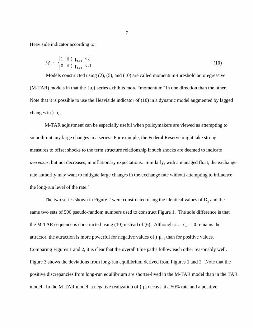
The Johansen (1996) procedure is not able to detect a long-run equilibrium relationship

between these two interest rates at conventional significance levels. In terms of equation (1), we let the

vector x consist of the logarithms of the federal funds and 10-year rates and included an intercept in thet

potential cointegrating vector. The multivariate AIC selected a model using two lagged changes of10

{)x } and the multivariate BIC selected a model with only 1-lagged change. If we use 1-lag of {)x },t t

the 8 (0) and 8 (0,1) statistics are 10.58 and 8.67 respectively. Instead, if we use the 2-lagtrace max

specification, the 8 (0) and 8 (0,1) statistics are 12.83 and 9.46 respectively. Since the respectivetrace max

90% critical values for these two test statistics are 15.66 and 12.91, it seems possible to conclude that

the rates are not cointegrated.

)µ̂t ' D1 µ̂t&1 % jp

i&1

(i) µ̂t&i % ,t

µ̂t&1

16

Following the Engle-Granger methodology, the estimated long-run equilibrium relationship (with

t-statistics in parenthesis) is:

r = -1.313 + 1.513r + µ (16)ft 10t t^

(-10.802) (27.251)

where: r and r are the logarithmic values of the, respectively. f 10

Next, we used the residuals of (16) to estimate a model of the form:

(17)

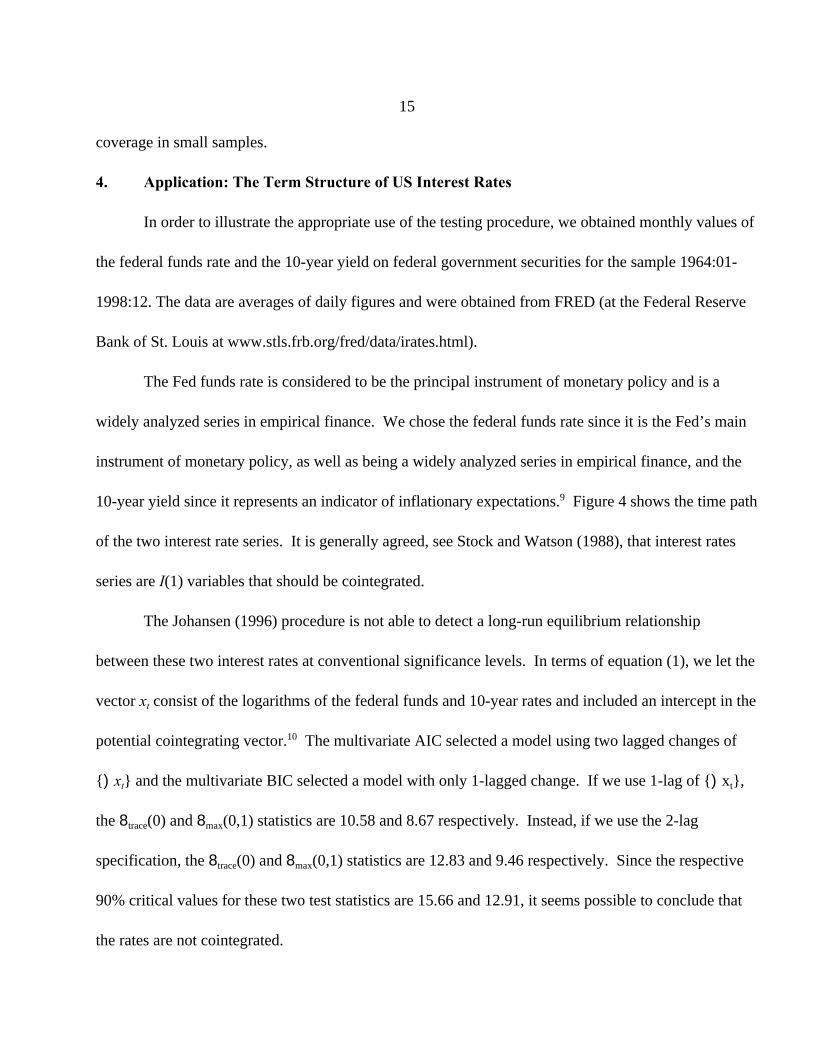
As shown in Table 7, the model using 2-lagged changes seems to be appropriate. In absolute

value, both values of ( have t-statistics exceeding 2.0. The key point to note is that the t-statistic fori11

the coefficient of is only -2.858. The Engle-Granger critical values at the 10%, 5% and 1%

significance levels are -3.03, -3.37 and -4.07, respectively. Hence, at conventional significance levels,

the Engle-Granger test indicates that the two interest rate series are not cointegrated.

Next, we estimated the residuals of (16) in the form of the TAR model using the threshold J =

0. As shown in the second column of Table 7, the point estimates for D = -0.085 and D = -0.0201 2

suggest convergence. However, the sample value of M = 4.32 is less than the 10% critical value12

(approximately 4.92) reported in Table 1. Moreover, the larger of the two t-values (equal to -1.582)

exceeds the 10% critical value for t-Max. Hence, at conventional significance levels, it is not possible

to reject the null hypothesis of no cointegration.

The third column of Table 7 reports results using an M-TAR model. As in the previous two

cases, diagnostic statistics suggest a model with two lagged changes of {)µ }. The sample value of the^t

M-statistic = 6.363 indicates that the null hypothesis D = D = 0 can be rejected near the 5%1 2

{)µ̂t}

Mt '1 if )µt&1 $&0.02610 if )µt&1 < &0.0261

17

significance level (As shown in Panel B of Table 1, the 5% critical value using 1-lagged change is

between 6.51 and 6.38. The critical value for 2-lagged changes is even smaller). Note that the point

estimates for D and D suggest substantially faster convergence for negative than for positive1 2

discrepancies from long-run equilibrium. Since the largest of the two t-statistics is only -0.628, we

cannot reject the null of no cointegration using the t-Max(M) test. However, this is not surprising given

the low power of the test. Given that the interest rates are cointegrated, the null hypothesis of symmetric

adjustment (i.e., D = D ) can be tested using a standard F-distribution. The sample value of F = 4.4181 2

has a p-value of 0.037 so that it is possible to reject the null hypothesis of symmetric adjustment. Also

note that the AIC indicated that the M-TAR model fits the data better than the Engle-Granger or the

TAR specifications.

Since we have little a priori knowledge about the true value of J, we can use Chan’s (1993)

method to find the consistent estimate of the threshold. When we searched over the possible thresholds

lying in the middle-70 percent of the arranged values of , we found that a threshold of -0.0261

results in the smallest residual sum of squares. As reported in the last column of Table 7, the M-TAR

model using the consistent estimate of the threshold (with t-statistics in parentheses) is:

)µ = -0.0201M µ - 0.141(1-M )µ + 0.186)µ - 0.155)µ + , (18)^ ^ ^ ^ ^t t t-1 t t-1 t-1 t-2 t

(-0.680) (-3.842) (2.790) (-2.312)

where:

(19)

Now, the point estimates of D and D suggest convergence such that the speed of adjustment is1 2

more rapid for negative than for positive discrepancies from J = -0.0261. The sample value M(M)* is

18

7.548 and the largest of the two t-statistics for the D equals -0.680. Hence, the M(M)* statistic allowsi

us to soundly reject the null hypothesis of no cointegration at the 5% significance level. Also note that

the F-test for symmetric adjustment can be just rejected at the 1% significance level. Hence, (18)

strongly suggests that the two interest rates are cointegrated and that the adjustment mechanism is

asymmetric. As measured by the AIC, the M-TAR model with the consistent estimate of the threshold

fits the data substantially better than the other models. Hence, the estimates suggest that discrepancies

from long-term equilibrium resulting from decreases in the federal funds rate or increases in the long-

rate (such that )µ < -0.0261) are eliminated relatively quickly whereas other changes display a larget-1

amount of persistence. This result is consistent with asymmetric federal reserve policy. An increase in

the long-rate (representing an increase in inflationary expectations) is met with policy adjustment

designed to decrease inflationary expectations. On the other hand, decreases in the long-rate are

allowed to persist.

The positive finding of cointegration with M-TAR adjustment justifies estimation of the following

error-correction model (with t-statistics in parentheses):

)r = -0.0020 - 0.0347M µ - 0.0274(1-M )µ + A (L))r + A (L))r + , (20)ft t t-1 t t-1 11 ft-1 12 10t-1 1t^ ^

(-0.504) (-1.418) (-0.922) F = 0.00 F = 0.0011 12

)r = -0.0003 - 0.0084M µ + 0.0648(1-M )µ + A (L))r + A (L) )r + , (21)10t t t-1 t t-1 21 ft-1 22 10t-1 2t^ ^

(-0.104) (-0.491) (3.121) F = 0.85 F = 0.0021 22

where: µ is obtained from (16), the Heaviside indicator is set in accord with (19), A (L) are first-^t-1 ij

order polynomials in the lag operator L, and F = p-value for the null hypothesis that both coefficientsij

of A are equal to zero. ij13

19

The t-statistics for the error-correction terms indicate that the federal funds rate is weakly

exogenous but that the long-rate adjusts to deviations from long-run equilibrium if µ < -0.0261. ^t-1

Notice that the 10-year rate adjusts in the “wrong” direction for positive values of )µ (although the^t-1

value of the t-statistic is only -0.491). The F-statistics indicate that the long-rate is not Granger-caused

by the short-rate but that lagged changes in both rates affect movements in the short-rate. However, an

important caveat concerns the fact that the estimates of the D are somewhat sensitive to the samplei.j

period. Moreover, since Hansen (1997) and Enders and Falk (1999) show that OLS estimates of the

speed of adjustment terms have poor small sample properties, we next consider the model using a

longer data set covering the 1954:7 - 1997:4 sample period. Unfortunately, we have no clear way of

determining whether the gains from using the longer sample outweigh the losses from estimating the

model over several policy regimes. Nevertheless, the estimated adjustment equation [i.e., the analogue

of equation (18)] is similar to that reported above:

)µ = -0.0135M µ - 0.2384(1-M )µ + 0.0102)µ - 0.0527)µ + 0.1618)µ + , (18')^ ^ ^ ^ ^ ^t t t-1 t t-1 t-1 t-2 t-2 t

(-0.694) (-8.298) (0.2326) (1.249) (3.861)

where: J is estimated to be -0.0383, the sample value of M(M)* is 34.56 and the F-statistic for the null

hypothesis D = D is 42.859 with a p-value of nearly zero. 1 2

The hypotheses D = D = 0 and D = D are both soundly rejected. Again the model suggests1 2 1 2

that negative discrepancies from long-run equilibrium (such that )µ < -0.0383) are eliminated rathert

quickly but that others are allowed to persist. However, the error-correction model using the entire

sample does have a different interpretation. Consider:

)r = -0.0029 - 0.0088M µ - 0.2266(1-M )µ + A (L))r + A (L))r + , (20')ft t t-1 t t-1 11 ft-1 12 10t-1 1t^ ^

(-0.733) (-0.464) (-8.232) F = 0.00 F = 0.0011 12

20

)r = 0.0013 + 0.0085M µ - 0.0016(1-M )µ + A (L))r + A (L) )r + , (21')10t t t-1 t t-1 21 ft-1 22 10t-1 2t^ ^

(0.887) (1.265) (-0.167) F = 0.16 F = 0.0021 22

For the longer sample period, the 10-year rate, but not the federal funds rate, appears to be

weakly exogenous. Instead, an increase in inflationary expectations and the long-rate such that )µ < -t-1

0.0383 induces an increase in the federal funds rate. The F-statistics still indicate that the long-rate is

not Granger-caused by the short-rate but that lagged changes in both rates affect movements in the

short-rate.

In contrast, if we assume symmetric adjustment, the error-correction model over the oft-studied

1979:10 - 1997:4 sample period is:14

)r = -0.0021 - 0.0318 µ + A (L))r + A (L))r + , (22)ft t-1 11 ft-1 12 10t-1 1t^

(-0.547) (-1.678) F = 0.00 F = 0.0011 12

)r = -0.0016 + 0.021µ + A (L))r + A (L))r + , (23)10t t-1 21 ft-1 22 10t-1 2t^

(-0.580) (1.569) F = 0.83 F = 0.0021 22

Except for the error-correction terms, the coefficient estimates in (22) and (23) are all similar to

those in (20) and (21). The key difference is that the symmetric adjustment assumption implies that

there is no convergence toward the long-run equilibrium; both error-correction terms are not significant

at conventional levels. Moreover, in spite of the fact that the M-TAR model contains an additional two

coefficients, the multivariate AIC selects the M-TAR model. The multivariate AIC equals -2555.89

for the M-TAR model of (20) and (21) and equals -2551.83 for the system given by (22) and (23).

5. Conclusions

The paper developed a generalization of the Engle-Granger (1987) procedure that allows for

either threshold autoregressive (TAR) or momentum-TAR (M-TAR) adjustment towards a

21

cointegrating vector. The power of the test for TAR adjustment is poor compared to that of the Engle-

Granger test. However, for a plausible range of the adjustment parameters, the power of the M-TAR

test can be many times that of the Engle-Granger test.

We chose to illustrate the appropriate use of the tests using short-term and long-term interest

rates. The Engle-Granger and TAR tests indicated that the Federal Funds rate and the 10-year yield

on government bonds are not cointegrated. However, models which permit M-TAR adjustment

indicate that the two rates are indeed cointegrated. Moreover, the M-TAR models fit the data

substantially better than that assume either symmetric or TAR adjustment.

22

References

Andrews, D. and W. Ploberger (1994). “Optimal Tests When a Nuisance Parameter is Present OnlyUnder the Alternative.” Econometrica 62, 1383-1414.

Balke, Nathan S. and T. Fomby (1997). “Threshold Cointegration.” International Economic Review38, 627 - 43.

Beaudry, Paul and Gary Koop (1993). “Do Recessions Permanently Change Output?” Journal ofMonetary Economics. 149-64.

Bradley, Michael and D. Jansen (1997). “Nonlinear Business Cycle Dynamics: Cross-CountryEvidence on the Persistence of Aggregate Shocks.” Economic Inquiry 35, 495-509.

Caner, Mehmet and Bruce Hansen (1998). “Threshold Autoregression with a Near Unit Root.”University of Wisconsin Working Paper: mimeo.

Chan, K. S. (1993). “Consistency and Limiting Distribution of the Least Squares Estimator of aThreshold Autoregressive Model.” The Annals of Statistics 21, 520 - 33.

Chan, K., and Howell Tong (1989). “A Survey of the Statistical Analysis of a Univariate ThresholdAutoregressive Model.” in Roberto Mariano (Ed.), Advances in Statistical Analysis andStatistical Computing: Theory and Applications, Volume 2 (JAI Press Inc.: Greenwich,Conn.), pp1-42.

DeLong, J. Bradford and Lawrence J. Summers (1986). “Are Business Cycles Symmetrical?” in R. J.Gordon, ed. The American Business Cycle (University of Chicago Press: Chicago).

Eitrheim, Øyvind., and Timo Teräsvirta (1996). “Testing the Adequacy of Smooth TransitionAutoregressive Models”, Journal of Econometrics, 74, 59-76.

Enders, Walter and C.W.J. Granger (1998). “Unit-Root Tests and Asymmetric Adjustment With anExample Using the Term Structure of Interest Rates.” Journal of Business and EconomicStatistics 16, 304 - 11.

Enders, Walter and Barry Falk (1999). “Confidence Intervals for Threshold Autoregressive Models.”Department of Economics Working Paper. Iowa State University.

Engle, Robert F. and C.W.J. Granger (1987). “Cointegration and Error Correction: Representation,Estimation and Testing”, Econometrica 55 (March): 251-76.

23

Falk, Barry (1986). “Further Evidence on the Asymmetric Behavior of Economic Time Series over theBusiness Cycle”, Journal of Political Economy 94 (October): 1096-1109.

Granger, Clive W.J., and Timo Teräsvirta (1993). Modelling Nonlinear Economic Relationships(Oxford: Oxford University Press).

Granger, C.W.J. and T.H. Lee (1989). “Investigation of Production, Sales, and InventoryRelationships using Multicointegration and Nonsymmetric Error-Correction Models.” Journalof Applied Econometrics 4, S145 - S159.

Hansen, Bruce (1996). “Inference When a Nuisance Parameter is Not Identified Under the NullHypothesis” Econometrica 64, 413-30.

_______ , (1997). “Inference in TAR Models.” Studies in Nonlinear Dynamics and Econometrics1. 119 - 31.

Johansen, Soren (1996). Likelihood-Based Inference in Cointegrated Vector Auto-RegressiveModels (Oxford: Oxford University Press).

Lukkonen, R., P. Saikkonen, and T. Teräsvirta (1988). “Testing Linearity Against Smooth TransitionAutoregressive Models”, Biometrika, 75, 491-99.

Neftci, Salih N. (1984). “Are Economic Time Series Asymmetric over the Business Cycle?” Journalof Political Economy 92, 307-28.

Nelson, C. R. and C. I. Plosser (1982). “Trends and Random Walks in Macroeconomic Time Series:Some Evidence and Implications.” Journal of Monetary Economics 10, 139-62.

Petrucelli, J. and S. Woolford (1984). A Threshold AR(1) Model. Journal of Applied Probability21, 270 - 86.

Pippenger, M. K. and G. E. Goering (1993), “A Note on the Empirical Power of Unit Root TestsUnder Threshold Processes.” Oxford Bulletin of Economics and Statistics 55, 473 - 81.

Ramsey, J. B. and P. Rothman (1996). “Time Irreversibility and Business Cycle Asymmetry.” Journalof Money, Credit and Banking 28, 1 - 21.

Sichel, D. (1993). “Business Cycle Asymmetry: A Deeper Look.” Economic Inquiry 31, 224- 36.

Siklos, Pierre and C.W.J. Granger (1997). “Regime Sensitive Cointegration with an Application toInterest Rate Parity.” Macroeconomic Dynamics 3, 640 - 57.

24

Stock, J. and M. Watson (1988). “Testing for Common Trends.” Journal of the AmericanStatistical Association 83, 1097 - 1107.

Teräsvirta, Timo and H. M. Anderson (1992) “Characterizing Nonlinearities in Business Cycles UsingSmooth Transition Autoregressive Models.” Journal of Applied Econometrics7, S119 -S139.

Tong, Howell (1990). Non-Linear Time-Series: A Dynamical Approach. (Oxford University Press:Oxford).

_________ (1983). Threshold Models in Non-Linear Time Series Analysis. (Springer-Verlag: NewYork).

Tsay, R. S. (1989). "Testing and Modeling Threshold Autoregressive Processes." Journal of theAmerican Statistical Association 84, 231 - 40.

25

Table 1: The Distribution of M

Panel A: TAR Adjustment

No Lagged Changes One Lagged Change Four Lagged Changes Obs. 90% 95% 99% 90% 95% 99% 90% 95% 99%

50 5.09 6.20 8.78 5.08 6.18 8.67 5.22 6.33 9.05100 5.01 5.98 8.24 4.99 6.01 8.30 5.20 6.28 8.82250 4.94 5.91 8.08 4.92 5.87 8.04 5.23 6.35 8.94500 4.91 5.85 7.89 4.88 5.79 7.81 5.21 6.33 9.09

Panel B: M-TAR Adjustment50 5.59 6.73 9.50 5.56 6.67 9.32 5.32 6.39 8.89100 5.45 6.51 8.78 5.47 6.51 8.85 5.20 6.20 8.46250 5.38 6.42 8.61 5.36 6.38 8.62 5.13 6.12 8.26500 5.36 6.35 8.43 5.32 6.28 8.40 5.06 6.05 8.31

Table 2: The Distribution of t-Max

Panel A: TAR AdjustmentNo Lagged Changes One Lagged Change Four Lagged Changes

Obs. 90% 95% 99% 90% 95% 99% 90% 95% 99%

50 -1.89 -2.12 -2.58 -1.92 -2.16 -2.64 -1.89 -2.14 -2.69100 -1.90 -2.11 -2.55 -1.91 -2.14 -2.57 -1.76 -1.98 -2.43250 -1.90 -2.12 -2.53 -1.90 -2.12 -2.53 -1.71 -1.91 -2.34500 -1.89 -2.11 -2.52 -1.90 -2.10 -2.51 -1.69 -1.89 -2.29

Panel B: M-TAR Adjustment50 -1.79 -2.04 -2.53 -1.82 -2.07 -2.57 -1.84 -2.10 -2.67100 -1.77 -2.02 -2.47 -1.79 -2.03 -2.49 -1.77 -2.00 -2.51250 -1.76 -1.99 -2.45 -1.77 -2.00 -2.44 -1.76 -1.99 -2.45500 -1.76 -1.98 -2.41 -1.75 -1.99 -2.42 -1.75 -1.98 -2.42

26

Table 3: Power Functions for the TAR Model1

The M Statistic The t-Max Statistic The Engle-Granger Test

D D 10% 5% 1% 10% 5% 1% 10% 5% 1%1 2

-0.02 -0.50 0.173 0.094 0.020 0.196 0.101 0.022 0.199 0.102 0.0175 0

-0.10 0.240 0.143 0.032 0.261 0.153 0.038 0.270 0.152 0.0280

-0.15 0.299 0.186 0.054 0.305 0.189 0.053 0.333 0.190 0.0470

-0.20 0.349 0.223 0.070 0.352 0.228 0.073 0.382 0.233 0.0620

-0.25 0.385 0.257 0.086 0.364 0.240 0.077 0.411 0.261 0.0720

-0.05 -0.10 0.405 0.251 0.070 0.429 0.280 0.083 0.570 0.274 0.0630 0

-0.15 0.522 0.357 0.117 0.533 0.368 0.122 0.570 0.375 0.1060

-0.20 0.610 0.436 0.175 0.582 0.421 0.169 0.646 0.453 0.1530

-0.25 0.682 0.516 0.228 0.637 0.473 0.205 0.718 0.526 0.2020

-0.10 -0.15 0.854 0.712 0.363 0.840 0.709 0.372 0.881 0.736 0.3400 0

-0.20 0.923 0.823 0.492 0.889 0.783 0.487 0.942 0.839 0.4660

-0.25 0.904 0.789 0.613 0.922 0.835 0.551 0.965 0.898 0.5750

Note: Each entry is the percentage of instances in which the null hypothesis of no cointegration wascorrectly rejected. For the test sizes of 10%, 5% and 1%, the statistic with the largest percentagecorrect is highlighted in boldface.

27

Table 4: Power Functions for the M-TAR Model1

The M Statistic The t-Max Statistic The Engle-Granger Test

D D 10% 5% 1% 10% 5% 1% 10% 5% 1%1 2

-0.02 -0.50 0.192 0.102 0.024 0.184 0.094 0.019 0.217 0.110 0.0175 0

-0.10 0.407 0.259 0.076 0.255 0.148 0.041 0.395 0.225 0.0490

-0.15 0.674 0.502 0.223 0.249 0.179 0.060 0.596 0.387 0.1070

-0.20 0.868 0.753 0.459 0.297 0.196 0.073 0.786 0.597 0.2190

-0.25 0.956 0.896 0.686 0.271 0.190 0.078 0.894 0.751 0.3610

-0.05 -0.10 0.476 0.303 0.094 0.373 0.234 0.069 0.512 0.322 0.0720 0

-0.15 0.743 0.574 0.257 0.408 0.291 0.113 0.730 0.532 0.1770

-0.20 0.902 0.794 0.495 0.414 0.299 0.135 0.869 0.719 0.3130

-0.25 0.973 0.927 0.729 0.422 0.321 0.149 0.958 0.875 0.5090

-0.10 -0.15 0.862 0.724 0.379 0.704 0.565 0.284 0.910 0.778 0.3570 0

-0.20 0.961 0.883 0.619 0.714 0.595 0.352 0.971 0.899 0.5600

-0.25 0.993 0.966 0.825 0.703 0.587 0.364 0.992 0.968 0.7480

Note: Each entry is the percentage of instances in which the null hypothesis of no cointegration wascorrectly rejected. For the test sizes of 10%, 5% and 1%, the statistic with the largest percentagecorrect is highlighted in boldface.

28

Table 5: The Distribution of M*

Panel A: TAR Adjustment

No Lagged Changes One Lagged Change Four Lagged Changes Obs. 90% 95% 99% 90% 95% 99% 90% 95% 99%

50 6.05 7.24 9.90 6.20 7.31 10.00 6.79 8.05 11.05100 5.95 6.95 9.27 6.02 7.08 9.51 6.35 7.41 9.88250 5.93 6.93 9.15 5.92 6.93 9.18 6.44 7.56 10.18

Panel B: M-TAR Adjustment50 5.97 7.12 9.96 5.99 7.14 9.93 5.99 7.11 9.79100 5.73 6.78 9.14 5.76 6.86 9.29 5.52 6.56 8.91250 5.58 6.62 8.82 5.57 6.63 8.84 5.32 6.32 8.47

Table 6: The Distribution of t-Max*

Panel A: TAR Adjustment

Obs. No Lagged Changes One Lagged Change Four Lagged Changes 90% 95% 99% 90% 95% 99% 90% 95% 99%

50 -1.62 -1.89 -2.43 -1.70 -1.97 -2.59 -1.78 -2.05 -2.65100 -1.61 -1.85 -2.35 -1.65 -1.90 -2.39 -1.66 -1.92 -2.44250 -1.59 -1.84 -2.31 -1.61 -1.86 -2.33 -1.52 -1.73 -2.30

Panel b: M-TAR Adjustment50 -1.65 -1.92 -2.44 -1.71 -1.98 -2.51 -1.72 -2.01 -2.60100 -1.65 -1.90 -2.37 -1.67 -1.94 -2.44 -1.65 -1.90 -2.42250 -1.66 -1.90 -2.36 -1.67 -1.91 -2.37 -1.66 -1.90 -2.37

29

TABLE 7: Estimates of the Interest Rate Differential[Sample: 1964:01-1998:12, monthly]

Engle-Granger Threshold Momentum Momentum-Consistent

D -0.068 -0.085 -0.021 -0.0201a

(-2.858 ) (-2.522) (-0.628) (-0.680)

D NA -0.020 -0.117 -0.1412a

(-1.582) (-3.526) (-3.842)

( 0.188 0.190 0.183 0.1861a

(-2.782) (2.787) (2.730) (2.790)

( -0.149 -0.147 -0.161 -0.1552a

(-2.197) (-2.153) (-2.376) (-2.312)

AIC 11.74 13.24 9.285 7.022b

M NA 4.32 6.363 7.548c

D = D NA 0.495 4.418 6.6981 2 d

(0.482) (0.037) (0.010)

Notesa. Entries are estimated value of D (or ( ) with the t-statistic in parentheses. i i

b. The AIC is calculated as: T*log(SSR) + 2*n where: T = number of usable observations, SSR = sum ofsquared residuals and n = number of regressors. c. Entries in this row are the sample values of N, N(M) or N*(M). d. Entries in this row are the sample F-statistic for the null hypothesis that the adjustment coefficients areequal. Significance levels are in parenthesis below.

Figure 1: Threshold Cointegration

50 100 150 200 250 300 350 400 450 500-16.0

-12.0

-8.0

-4.0

0.0

4.0

8.0

12.0x(1)

x(2)

30

Figure 2: Momentum Cointegration

50 100 150 200 250 300 350 400 450 500-16.0

-12.0

-8.0

-4.0

0.0

4.0

8.0

12.0x(1)

x(2)

31

Figure 3: The Error Correction Terms

50 100 150 200 250 300 350 400 450 500-7.5

-5.0

-2.5

0.0

2.5

5.0

7.5TAR

M_TAR

32

0

5

10

15

20

55 60 65 70 75 80 85 90 95

Fed funds rate10 year yield

Pe

rce

nt

(monthly)

33

Figure 4 Interest Rate Data

34

1. Balke and Fomby (1997) posit a framework in which adjustment towards long-run equilibriumoccurs when a shock creates a disequilibrium error exceeding some threshold. However, if the extentof the disequilibrium is “small”, there may be no convergence towards the long-run relationship. Thus,in a 2-variable system, the long-run relationship is given by a band instead of a line. The intuition is thatadjustment costs prevent complete convergence to the long-run relationship.

2. Of course, it is possible to allow )µ to display asymmetric adjustment to its lagged changes. Fort

example, the magnitude of each ( could depend on whether )µ was positive or negative. Moreover,i t-1

as discussed in Granger and Teräsvirta (1993), the values of D and D can be allowed to smoothly1 2

adjust over time.

3. Caner and Hansen (1998) present a purely statistical argument for M-TAR adjustment. If µ is at-1

near unit root process, setting the Heaviside indicator using )µ can perform better than thet-1

specification using pure TAR adjustment.

4. This pattern would be reversed if # D # ># D #.1 2

5. For example, if the two t-statistics are -2.5 and -1.5, t-Min is -2.5 and t-Max is -1.5. Recall thatthe necessary conditions for convergence are for D and D to be negative. Thus, the t-Max statistic is1 2

a direct test of these conditions. The M-statistic can lead to a rejection of the null hypothesis D = D = 01 2

when only one of the values is negative. However, as shown below, the M-statistic is quite useful sinceit can have substantially more power than the t-Max statistic. Nevertheless, the M-statistic should beused only in those cases where the point estimates for D and D imply convergence. The t-Min statistic1 2

was found to have very little power and is not reported here.

6. We have also generated critical values for the three variable case. These are reported in anAppendix that is available from the authors on request.

7.The critical values are reasonably insensitive to the level of serial correlation in {x }. For example, asit

shown in Tables 1 and 2, with 100 observations and one lagged change such that * = * = 0.6, the t-1 2

Max statistic is -2.14, and the M- statistic is 6.01. Respectively, for * = * = 0.1 and * = * = 0.8,1 2 1 2

the t-Max statistic is -2.14 and -2.12, while the M-statistics are 5.95 and 6.05. However, for * = 0.11

and * = 0.6, the critical values for t-Max and M are -2.10 and 5.72, respectively. Finally, for * = 0.02 1

and * = 0.8, the critical values for t-Max and M are -2.09 and 5.69, respectively. A table of the2

various critical values is available from the authors upon request.

8. Also note that the power of the t-Max statistic is usually superior to that of the M-statistic when thesize of the test is 1% and there is a reasonable amount of asymmetry.

9. In previous versions of this paper we examined other US short-term and long-term interest rateseries as well as a sample going back to 1959. The results are not shown to conserve space. More

Endnotes

35

often than not we conclude that some form of asymmetric adjustment exists between short and longrates of differing maturities.

10. Once again, all tests were also conducted using interest rate levels. One attraction of the logtransformation, in the present context, is that it treats changes in interest rates differently when levels arelow than when they are high. Hence, a change in the Fed funds rate from 3 to 3.5% (change =.5%) ismuch larger when the log transformation is used than a .5% change from, say, 15 to 15.5%. In anyevent, our findings of asymmetric adjustment were largely unaffected by this consideration.

11. The Ljung-Box Q-statistics using 4,8, and 12 lagged autocorrelations have a p-value lower than0.60 and residual autocorrelations (not shown in the Table) never exceed 0.10 in absolute value.

12. Diagnostic checking of the residuals indicates that the model with 2-lagged changes is appropriate.

13. The estimated model using only 1-lagged change of each variable is quite similar to the modelreported here.

14.This is the sample marking the beginning of new Federal Reserve operating procedures.