Embed Size (px)
Citation preview

Automatic Frontal Face Recognition System Based on
Wavelet Decomposition and Support Vector Machines
by
Wang Wei
Doctoral thesis approved by the Graduate School of Advance
Technology and Science for the degree of
Doctoral of Engineering
in
Department of Systems Innovation Engineering
September 2013
The University of Tokushima

Abstract
Automatic Face Recognition (AFR) aims at identifying different human
beings according to their face images. Such research has both significant
theoretic values and wide potential applications. As a scientific issue, AFR
is a typical pattern analysis, understanding and classification problem,
related to Pattern Recognition, Computer Vision and Cognitive Psychology
etc. Its achievements would contribute to the development of these
disciplines.
After more than 30 years’ development, AFR has made great progress
especially in the past ten years. The state-of-the-art AFR system can
perform identification successfully under well-controlled environment.
However, a great number of challenges are to be solved before one can
implement a robust practical AFR application. The following key issues are
especially pivotal: (1) the accurate facial feature location problem; (2)
efficient face representation and corresponding classifier with high
accuracy; (3) how to improve the robustness of AFR to inevitable
mis-alignment of the facial feature. In addition, system design is also as
important for developing robust and practical AFR systems. In this thesis,
the above-mentioned key issues are studied, aiming at practical automatic
frontal face recognition (AFFR) system. And the main contribution of this
thesis includes:
1. A novel fast fractal image compression
A novel fast fractal image coding algorithm based on texture feature is
proposed. The most fractal image encoding time is spent on determining
the approximate D-block from a large D-blocks library by using the global
searching method. Clustering the D-blocks library is an effective method to
reduce the encoding time. First, all the D-blocks are clustered into several
parts based on the new texture feature alpha derived from variation
function; second, for each R-block, the approximate D-blocks are searched
for in the same part. In the search process, we import control parameter δ,
this step avoids losing the most approximate D-block for each R-block.
Finally, the R-blocks whose least errors are larger than the threshold given

in advance are coded by the quad tree method. The experimental results
show that the proposed algorithm can be over 6 times faster compared to
the moment-feature-based fractal image algorithm; in addition, proposed
algorithm also improves the quality of the decoded image as well increases
the PSNR’s average value by 2 dB.
2. Provided a thorough survey of the AFR history
The latest AFR survey was published in the year 2000, which in fact
surveyed the AFR researches before 1999. This thesis has provided a more
recent overview of the AFR research and development. Then, AFR
methods are further categorized according to facial feature extraction, face
representation, and classification separately. We also survey the main
public face databases and performance evaluations protocols, based on
which the state-of-the-arts of AFR are summarized. Finally, the challenges
and technical trends in AFR fields are discussed.
3. Proposed an eye location algorithm based on HSV color space and
template matching
The quality of feature extraction will directly affect recognition results.
Eyes are the one of the most important organs of a face including a lot of
useful features. Therefore, eye location has become one of the most
significant techniques in pattern recognition.
This thesis proposed an eye location method based on the HSV color
space model using template matching. At first, we describe an
implementation for skin detection which relies on the H channel to
characterize the skin colors range, and determine the possible face region.
Then we manually extract an average eye template using the human eye’s
sample images, and finally in the face region, locate the eyes using this
average template. As eye template matching, the rectangular region of the
eye which confirmed from the skin region is just searched. Compared to
other template matching methods that search for the human eye in whole
face region, the proposed method saves on the matching time by avoiding
the impact of the mouth and nose in the process of positioning.
Undoubtedly, this method enhances the accuracy of eye detection.
4. Investigated the face detection methods, and proposed an improved
training AdaBoost algorithm for face detection

Face detection technology as an important part of face recognition has
high research and application value. In 2001 the AdaBoost algorithm was
applied to face detection by Paul Viola and Michael Jones. The AdaBoost
is an algorithm for constructing a strong classifier as linear combine of
weak classifier trained by different training sets. The classifiers can be
weak (i.e., display a substantial error rate), but their performance is not
random (resulting in an error rate of 0.5 for binary classification), they will
improve the final model.
In this section, an improved training algorithm for AdaBoost is proposed
to bring down the complexity of human face detection. Two methods are
adopted to accelerate the training: (1) A method to solve the parameters of
a single weaker classifier is proposed, making the training speed is higher
than probability method; (2) a double threshold decision for a single
weaker classifier is introduced, and the number of weaker classifiers in the
AdaBoost system is reduced. Based on the simplified detector, both the
training time and the detecting time could be reduced.
5. Primarily studied wavelet transform based feature extraction and
Support vector machines to face recognition problem; recognition
rate is analyzed and evaluated experimentally
The extracted features from human images by wavelet decomposition are
less sensitive to facial expression variation. As a classifier, SVM provides
high generation performance without transcendental knowledge. First, we
detect the face region using an improved AdaBoost algorithm. Second, we
extract the appropriate features of the face by wavelet decomposition, and
compose the face feature vectors as input to SVM. Third, we train the SVM
model by the face feature vectors, and then use the trained SVM model to
classify the human face. In the training process, three different kernel
functions are adopted: Radial basis function, Polynomial and Linear kernel
function. Finally, we present a face recognition system that can achieve
high recognition precision and fast recognition speed in practice.
Experimental results indicate that the proposed method can achieve
recognition precision of 96.78 percent based on 96 persons in Ren-FEdb
database that is higher than other approaches.

Acknowledgment
I would like to express the deepest appreciation to all my friends. This
PhD thesis could not have been completed without the help of some
important and special people.
First and foremost, thanks to Professor Dr. Kenji Terada, my supervisor.
Thank you for encouragement and a great research environment. Without
your support and guidance this dissertation would not have been possible.
Thank you for providing me with all the necessary facilities.
To Dr. Akinori Tsuji, thanks for not only your help and good comments
but also for being a good friend.
To Dr. Karungaru, thanks for your professional advice.
In addition, a thank you to Professor Fuji Ren, who introduced me to
B1 lab, and whose help had lasting effect.
I’d also like to thank all B1 lab members, thanks for happy time in three
years.
I would like to express my gratitude towards my parents and sister for
their kind co-operation and encouragement which help me insist on to
finish with school.
I am thankful to and fortunate enough to get constant encouragement,
support and guidance from all of you who helped me in successfully
completing my dissertation. Also, I would like to extend my sincere regards
to all the staffs of Tokushima University for their timely support.

Contents
ABSTRACT………………………………….…………………………… I
ACKNOWLEDGMENTS…………………....……………………………V
CHAPTER I .................................................................................................. 1
INTRODUCTION ......................................................................................... 1
1.1 Introduction to Fractal Theory and Its Self-Similarity ........................ 1
1.1.1 Fractal Theory ................................................................................ 1
1.1.2 Self-Similarity ................................................................................ 2
1.2 Fractal Image Compression.................................................................. 4
1.3 Description of Automatic Face Recognition Problem ......................... 5
1.4 Face Recognition Research Significance and Typical Applications .... 7
1.5 Advantages and Disadvantages Using face as Biometric Identification
.................................................................................................................... 8
1.5.1 The Advantage of Face Recognition Technology .......................... 8
1.5.2 Disadvantage of Face Recognition Technology ............................. 9
1.6 Human visual recognition system characterization ........................... 10
1.7 Problem introduction and main contribution of this thesis ................ 13
1.7.1 Problem introduction .................................................................... 13
1.7.2 Main contribution of this thesis ................................................... 15
1.8 Organization of the Thesis ................................................................. 17
CHAPTER II ............................................................................................... 18
FRACTAL IMAGE COMPRESSION BASED ON TEXTURE
FEATURE ................................................................................................... 18
2.1 Architecture of the Proposed Novel Fractal Image Coding System and
the Variation Function .............................................................................. 19
2.1.1 Fractal Image Encoding Process .................................................. 19
2.1.2 Fractal Image Decoding Process .................................................. 23
2.1.3 Variation Function ........................................................................ 24
2.2 Proposed Novel Fast Fractal Image Coding Algorithm Based on
Texture Feature ......................................................................................... 27
2.2.1 Clustering Method based on Texture Feature .............................. 27
2.2.2 Solving the Clustering Error ........................................................ 28
2.3 Experimental Results and Discussion ................................................ 29
CHAPTER III .............................................................................................. 36
REVIEWS OF FACE RECOGNITION RESEARCH................................ 36
3.1 General Computational Model of Face Recognition ......................... 36
3.2 Research History and Present Research Situation ............................. 38
3.3 Main Technical Classification of Face Recognition .......................... 42
3.4.1 The major public face image database ......................................... 46
3.4.2 FERET Testing ............................................................................. 51
3.4.3 FRVT2000 and FRVT2002 testing .............................................. 51
3.5 Some Open Problems and Possible Technology Trends .................... 52
3.5.1 Some Open Problems ................................................................... 52
3.5.2 Possible Technology Trends ......................................................... 53
3.6 Summarize Development Situation ................................................... 54
CHAPTER IV ............................................................................................. 56
EYE LOCATION AND IMPROVED FACE DETECTION ALGORITHM
BASED ON ADABOOST .......................................................................... 56
4.1 Overview of Eye Location and Face Detection ................................. 56
4.2 Template Matching and Skin Detection Using HSV Space ............... 57
4.2.1 Eye Template Matching ............................................................... 57
4.2.2 Face Region Normalization.......................................................... 59
4.3 Summaries AdaBoost Algorithm and Proposed Improved AdaBoost
Algorithm for Face Detection .................................................................. 60
4.4 Experiments and Results .................................................................... 61
4.4.1 Eye Location Experimental Results ............................................. 61
4.4.2 Face Detection Experimental Results .......................................... 63
CHAPTER V ............................................................................................... 64
PRIMARILY STUDIED WAVELET BASED FEATURE EXTRACTION
AND SUPPORT VECTOR MACHINES ................................................... 64
5.1 Wavelet Transform Analysis Method ................................................. 64
5.1.1 Formal Definition of Wavelet Transform ..................................... 64
5.1.2 Discrete Wavelet Transform ......................................................... 65
5.1.3 Continuous Wavelet Transform .................................................... 69
5.2 Support Vector Machines ................................................................... 70
5.2.1 Linear SVM .................................................................................. 70
5.2.2 Nonlinear Classification ............................................................... 72
5.3 Proposed Method based on Wavelet Transform Method and SVM .. 73
5.3.1 Facial Feature Extraction based on Wavelet Transformation
Method................................................................................................... 73
5.3.2 Classification based on SVM ....................................................... 74

5.4 Experiments and Results .................................................................... 75
CHAPTER VI .............................................................................................. 79
CONCLUSIONS AND FUTURE WORK.................................................. 79
6.1 Conclusions ........................................................................................ 79
6.2 Future Work ........................................................................................ 81
REFERENCES ............................................................................................ 83

List of Figures
Figure Page
1 The Self-Similarities. 3
2 The Koch Curve. 4
3 Thatcher Illusions. 11
4 Example caricatures of some popular stars. 12
5 Flowchart of fractal image encoding. 22
6 Comparison PSNR and iterations. 23
7 δ vs. encoding time. Using the y-axis points as the
criterion, the curves are Lena, Camera, Goldhill, Bird,
Peppers, Boat, Barb from top to bottom in turn.
30
8 K vs. encoding time. Using the left points as the
criterion, the curves are Barb, Bird, Lena, Goldhill,
Camera, Boat, and Peppers from top to bottom in turn.
31
9 PSNR Comparison with Tan et al. [TY03]. The star
curve represents the novel fast fractal image coding
algorithm, and the triangle curve represents the Tan et
al. [TY03] respectively.
32
10 Decoded image with D-block size of 8×8. 32
11 Encoding time Comparison with Chen et al. [CZ04].
The star curve represents the novel fast fractal image
coding algorithm, and the triangle curve represents the
Chen et al. [CZ04] respectively.
33
12 Rate-distortion curve. The triangle curve represents
the novel fast fractal image coding algorithm, and the
star curve represents the Tan et al. [TY03]
respectively.
34
13 The results for the Peppers, Gledhill, Bird, Boat,
Camera and Barb with D-block size of 8×8.
35
14 Factors affect the appearance of face images. 53
15 Same Image in HSV. 57
16 An Intermediary. 57

17 The Result of Skin Detection. 57
18 Left and Right Synthetic Eye Templates. 58
19 Rectangular of Eye Region. 59
20 Face detection flow chart. 60
21 Some Examples for Binary Faces without Spectacles. 61
22 Results of eye detection without Spectacles. 62
23 Some Results of Eye Location with Expressionless
Images.
62
24 Results of Expressive Images, the Original Images of
These Examples Expressing Various Expressions.
62
25 Error Recognition Examples. 63
26 Detection results using AdaBoost. 63
27 Fig.27. Examples of facial images for
two-dimensional wavelet decomposition with depth 2.
74
28 Classification schemes of SVM. 75
29 The Face Detecting and Tracking using SURF
Method. (In this system, capture the video from the
second frame, nearer to the second frame, the more
feature points lines)
77
30 Automatic Frontal Face Recognition System interface. 78

List of Tables
Table Page
1 Typical Applications of Face Recognition. 8
2 Eight Basic Transformations. 21
3 PSNR results comparison with different text images. 34
4 A Brief History of Face Recognition Research. 39
5 Main approaches for face alignment. 43
6 Main approaches for face representation. 44
7 Main approaches for discrimination and classification. 45
8 Comparison of Different Face Databases. 48
9 Some new trends in AFR. 54
10 Comparison Recognition Rates. 76
11 Comparison Experimental Results. 77

1
CHAPTER I
INTRODUCTION
1.1 Introduction to Fractal Theory and Its Self-Similarity
In the most generalized terms, a fractal demonstrates a limit. Fractals
model complex physical processes and dynamical systems. The underlying
principle of fractals is that a simple process that goes through infinitely
much iteration becomes a very complex process. Fractals attempt to model
the complex process by searching for the sim
ple process underneath. Most fractals operate on the principle of a
feedback loop. A simple operation is carried out on a piece of data and then
fed back in again. This process is repeated infinitely many times. The limit
of the process produced is the fractal.
1.1.1 Fractal Theory
The word "fractal" often has different connotations for laypeople than
mathematicians, where the layperson is more likely to be familiar with
fractal art than a mathematical conception. The mathematical concept is
difficult to formally define even for mathematicians, but key features can
be understood with little mathematical background.
The feature of "self-similarity", for instance, is easily understood by
analogy to zooming in with a lens or other device that zooms in on digital
images to uncover finer, previously invisible, new structure. If this is done
on fractals, however, no new detail appears; nothing changes and the same
pattern repeats over and over, or for some fractals, nearly the same pattern
reappears over and over. Self-similarity itself is not necessarily
counter-intuitive (e.g., people have pondered self-similarity informally such
as in the infinite regress in parallel mirrors or the homunculus, the little
man inside the head of the little man inside the head...). The difference for
fractals is that the pattern reproduced must be detailed [MB83, HS12].

2
Almost all fractals are at least partially self-similar. This means that a
part of the fractal is identical to the entire fractal itself except smaller.
Fractals can look very complicated. Yet, usually they are very simple
processes that produce complicated results. And this property transfers over
to Chaos Theory. If something has complicated results, it does not
necessarily mean that it had a complicated input. Chaos may have crept in
(in something as simple as round-off error for a calculation), producing
complicated results. Fractal Dimensions are used to measure the
complexity of objects. We now have ways of measuring things that were
traditionally meaningless or impossible to measure.
Finally, Fractal research is a fairly new field of interest. Thanks to
computers, we can now generate and decode fractals with graphical
representations. One of the hot areas of research today seems to be Fractal
Image Compression. Many web sites devote themselves to discussions of it.
The main disadvantage with Fractal Image Compression and Fractals in
general is the computational power needed to encode and at times decode
them. As personal computers become faster, we may begin to see
mainstream programs that will factually compress images.
A fractal is a mathematical set that has a fractal dimension that usually
exceeds its topological dimension[MB04] and may fall between the
integers [MB83]. Fractals are typically self-similar patterns, where
self-similar means they are "the same from near as from far".[GJ96]
Fractals may be exactly the same at every scale, or, as illustrated in Figure
1, they may be nearly the same at different scales
[MB83][FK03][BJ92][VT92]. The definition of fractal goes beyond
self-similarity per se to exclude trivial self-similarity and include the idea
of a detailed pattern repeating itself [MB83][HS12].
1.1.2 Self-Similarity
An object is self-similar only if you can break the object down into an
arbitrary number of small pieces, and each of those pieces is a replica of the
entire structure. Some examples of self-similarity follow. The red outlining
indicates a few of the self-similarities of the object as shown Fig.1.

3
Fig. 1 The Self-Similarities.
Mandelbrot [MB83] offers the following definition of a fractal: A
fractal is a set for which the Hausdorff-Besicovitch dimension exceeds its
topological dimension. This definition, although correct and precise, is too
restrictive, since it excludes many fractals that are useful in physics [FJ89].
An alternative definition is given by Mandelbrot in [MB86]. A fractal is
a shape made of parts similar to the whole. This definition uses the concept
of self-similarity. A set is called strictly self-similar if it can be broken into
arbitrary small pieces, each of which is a small replica of the entire set.
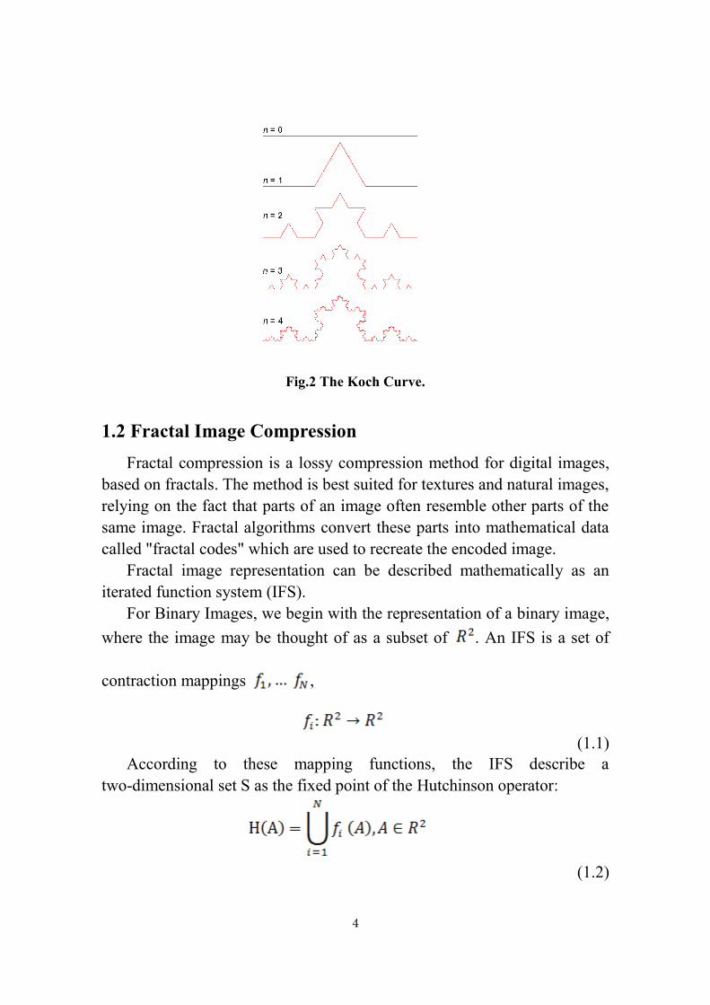
Fig. 2 show the construction of the Koch curve. It begins with a line. In
the first step the middle third is replaced by an equilateral triangle and the
baseline is removed. This procedure is applied repeatedly to the remaining
lines. In the limit there is a strictly self-similar structure. Each fourth of this
structure is a rescaled copy of the entire structure.
4
Fig.2 The Koch Curve.
1.2 Fractal Image Compression
Fractal compression is a lossy compression method for digital images,
based on fractals. The method is best suited for textures and natural images,
relying on the fact that parts of an image often resemble other parts of the
same image. Fractal algorithms convert these parts into mathematical data
called "fractal codes" which are used to recreate the encoded image.
Fractal image representation can be described mathematically as an
iterated function system (IFS).
For Binary Images, we begin with the representation of a binary image,
where the image may be thought of as a subset of . An IFS is a set of
contraction mappings ,
(1.1)
According to these mapping functions, the IFS describe a
two-dimensional set S as the fixed point of the Hutchinson operator:
(1.2)

5
That is, H is an operator mapping sets to sets, and S is the unique set
satisfying H(S) = S. The idea is to construct the IFS such that this set S is
the input binary image. The set S can be recovered from the IFS by fixed
point iteration: for any nonempty compact initial set A0, the iteration Ak+1 =
H(Ak) converges to S.
The set S is self-similar because H(S) = S implies that S is a union of
mapped copies of itself:
(1.3)
So we see the IFS are a fractal representation of S.
IFS representation can be extended to a grayscale image by considering
the image's graph as a subset of R3. For a grayscale image u(x,y), consider
the set S = {(x,y,u(x,y))}. Then similar to the binary case, S is described by
an IFS using a set of contraction mappings ƒ1,...,ƒN, but in R3,
fi:R3→R
3 (1.4)
A challenging problem of ongoing research in fractal image
representation is how to choose the ƒ1,...,ƒN such that its fixed point
approximates the input image, and how to do this efficiently. A simple
approach [FY92] for doing so is the following:
Step 1: Partition the image domain into blocks Ri of size s×s.
Step 2: For each Ri, search the image to find a block Di of size 2s×2s that is
very similar to Ri.
Step 3: Select the mapping functions such that H(Di) = Ri for each i.
In the second step, it is important to find a similar block so that the IFS
accurately represents the input image, so a sufficient number of candidate
blocks for Di need to be considered. On the other hand, a large search
considering many blocks is computationally costly. This bottleneck of
searching for similar blocks is why fractal encoding is much slower than
for example DCT and wavelet based image representations.
1.3 Description of Automatic Face Recognition Problem
Human being seems to have “inherent” face recognition capabilities, to
give the computer the same ability is one of the dream of human being, this
is called automatic face recognition (hereinafter referred to as AFR). If we
take the camera, image scanner, etc. as the computer’s “eyes”, digital

6
images can be seen as a computer “images”, in short, AFR studies have
attempted to give computes the ability to recognize people identity
according to the facial images they see. Broadly speaking, this recognition
ability includes the following different functions:
(1) Face detection and tracking
Face detection tasks require the computer to judge whether there is face
in the “images” observer by “eyes”. If there is, we need to give its
coordinate position, size information of the face region in the image at the
same time. Face tracking needs further output the continuous changes of
the detected face position, size, etc. along with time.
(2) Facial feature detection and extraction
This task requires determining the facial image in the eyes, nose, mouth
and other organs, also describing the shape information of these organs and
their facial contour.
(3) Face classification
According to the result of facial feature detection and extraction,
combing with facial image luminance distribution information, judge the
gender, facial expression, race, age and other attributes of the detected
human face.
(4) Identification based on face image comparison
That is usual sense of the problem of face recognition. This includes
two types of recognition: one is close set face recognition, assume that the
input face must be an individual in the face database; another one is open
set face recognition, first of all, determine whether the input face is in the
database, if it is, then identify it.
Development of face recognition allows an organization into three
types’ algorithms: frontal, profile, and view tolerant recognition. Frontal
recognition is the classical approach. Profile schemes as stand-alone
systems have a rather marginal significance for identification. Face
recognition can be formulated as: given a static or video image, to identify
or verify persons in the scene by comparing with faces stored in the
database.

7
1.4 Face Recognition Research Significance and Typical
Applications
Face recognition research began in the late 1960s [CB65, GH71, Ka73,
KB76, HH77, HK81], nearly 40 years has been received the considerable
development. Especially in recent years, it has become a hot research topic,
domestic and abroad well-known universities, research institutions and IT
companies get a lot of projects support. Face recognition are taken seriously,
because it has important research significance, outstanding performance in
two aspects: contribution to the development of discipline and enormous
potential applications.
(1) Face recognition can greatly promote the development of many related
disciplines.
AFR as a typical image pattern analysis, understanding and
classification calculations problem, it provides a good specific issues for
pattern recognition, image processing, analysis and understanding,
computer vision, artificial intelligence, human-computer interaction,
computer graphics, cognitive science, neural computation, physiology,
psychology and other disciplines[Ve98, BR02, BT03]. Again, as a
computer vision problem, how to integrate the general prior shape
information of human faces to accurately restore specific 3D face structure.
It is a very valuable research issue [Sh97, GB00, BJ01, Ra02].
(2) Face recognition as a biometric identification technology has great
potential application prospect.
Information security, information networks is becoming more and more
popular. This brings people more benefits, also brings serious security
issues of information acquirement and access. And face recognition as
typical biometric identification technology, its natural and high
acceptability, etc. can be applied to all walks of life. Table 1 summarizes
some typical applications of face recognition.

8
Table 1 Typical Applications of Face Recognition.
Areas Specific applications
Entertainment Video game, virtual reality, training programs
Human-robot-interaction, human-computer-interaction
Smart cards Drivers licenses, entitlement programs
Immigration, national ID, passports, voter registration
Welfare fraud
Information security TV parental control, personal device logon, desktop logon
Application security, database security, file encryption
Intranet security, internet access, medical records
Secure trading terminals
Law enforcement and
surveillance
Advanced video surveillance, CCTV control
Portal control, post event analysis
Shoplifting, suspect tracking and investigation
1.5 Advantages and Disadvantages Using face as Biometric
Identification
As mentioned earlier, there are many kinds of biological characteristics
identification methods. But their security, reliability and other performance
have their merits in terms of authentication. Among them, face recognition
is the most important method to identify each other.
1.5.1 The Advantage of Face Recognition Technology
Compared with other biometric identification technology, face
recognition technology has unique advantage in terms of usability.
Furthermore, face recognition can be completed without any explicit action,
participation on the part of the user since face image can be acquired from
some distance by camera. Face recognition technical advantages embodied
in the following:

9
(1) It could covert operation, especially for security monitoring
This is applicable to solve important security issues, offender
monitoring, cyber pursuit and other applications. This is the fingerprint; iris,
retina and other biometric identification technology cannot be compared;
(2) Non-contact acquisition, no intrusive, and easy to be accepted
Therefore, it will not cause physical injury to the user, and conform to
the general user’s habits;
(3) Convenient, fast and powerful tracking ability
Face-based authentication system could record and save the client’s
facial while the event occurs, which can ensure the system has good
tracking ability.
(4) Low cost image acquisition device
At present, middle and low-grade USB CCD/CMOS camera prices
have been low, basically become standard peripherals, greatly expanded the
practical space; in addition, digital cameras, photo scanners and other
camera equipment, etc. have been more popularity, this further increase its
availability;
(5) More in line with recognition habits of human, interactivity is strong
For example, for fingerprints and iris recognition system, the general
user to identify is often powerless; but for human face, authorized user
interaction and cooperation can greatly improve the system reliability and
availability.
1.5.2 Disadvantage of Face Recognition Technology
However, the human face as a biometric identification technology also
has its inherent defects, this mainly reflected in:
(1) Poor stability of facial features
Despite the face usually don’t change radically (except for intentional
cosmetic), but face is strong plasticity of three-dimensional flexible skin
surface; it will be changed as the changes of expression and age, etc. The
skin characteristics also will be changed with age, makeup and cosmetic,
accidental injury;

10
(2) Low reliability and security
Although different individuals have different faces, overall the human
face are similar, and there are so many population on the earth. The
different between people face is very subtle, to achieve safe and reliable
authentication is quite difficult;
(3) Image acquisition is affected by various external conditions, therefore
the recognition performance is low
These disadvantages make face recognition become a very difficult
challenge. Especially if the user does not cooperate, the non-ideal
conditions, face recognition problem become the current hotter issue. At
present, the world best face recognition system only in the ideal situation
like user cooperation, the ideal acquisition condition, can basically meet the
requirements of general application [PM00, PG03].
1.6 Human visual recognition system characterization
Let the computer has automatic, fast and accurate face recognition
ability same as human visual system, it is a dream for researchers. Human
visual recognition system naturally becomes AFR frame of reference and
bionic foundation. This section simple introduced in literature [CW95,
ZCR00] the characteristics of human visual recognition system, looking
forward to having referential significance for AFR study.
(1) Is face recognition a specific process? [ZCR00]
Whether the human face recognition mechanism is quite different from
other general object recognition? In the human cerebral cortex, is there a
dedicated face recognition area? This is one of the focus problems that
many researchers have argued for a long time.
However more researchers argue that face recognition system is a
special process, it completes this particular object recognition by
specialized corresponding cortex. This argument most convincing evidence
is “prosopagnosia”. Person suffering from this disease could be normal to
identify other objects, even identify nose, eyes, mouth and other facial
organs; but cannot recognize familiar faces. So it is reasonable to doubt its
face recognition function area was destroyed.

11
(2) Global features and local features, which is more important?
Global features mainly include human face skin-color feature (such as
white, black), the overall profile (such as round face, oval face, square face,
long face, etc.), as well as the distribution of facial features. And local
features is refers to the characteristics of facial features, for example thick
eyebrows, the phoenix eye, crooked nose, mustache beard, pointed chin, etc.
and some exotic facial features, such as moles, scars, dimple and so on. A
widely accepted view is that: both are necessary for identification, but the
global features are generally used to rough matching, the local feature
provides more detailed confirmation. But one must be mentioned
phenomenon is: if there is a unique local feature (such as scar, mole, etc.),
it will first be used to determine the identity. The most important
experimental support for global features is called “Thatcher Illusion”, as
shown in Fig.3. Where a and b are the inverted images of Thatcher.
Although the images are inverted, we can still be easy to determine both
are Mrs. Thatcher’s faces, they look very similar. But in fact, their
difference is big: in b, its eyes and mouth are inverted. It is relatively seen
from c (a inverted) and d (b inverted).
(a) (b)
(c) (d)
Fig. 3 Thatcher Illusions.

12
Fig. 4 Example caricatures of some popular stars.
(3) The importance of facial features for recognition [ZCR00]
Different facial areas play different important role on the face
recognition. Generally considered, facial contours, eyes, mouth and other
features are more important for face recognition. The change of hairstyle
for face recognition is also important. But it is worth noting that the
hairstyle is available, especially for young people and women. Furthermore,
nose in the profile face recognition is more important than other
characteristics. That is mainly because in the profile face recognition, nose
region contains several key feature points.
(4) Caricatures’ enlightenment
We often can see the caricatures.Fig.4 shows caricatures of some
popular stars. It is easy to see: caricatures deliberately exaggerated the most
important personalized facial features. These features further deepened out
understanding of facial characters, making us easier to remember their
faces.
In fact this is what the AFR system should extract “unusual”
personalized features. The most direct approach is to extract those features
which deviate from the average face. AFR method based on Fisherface is
trying to extract different features between the different faces for final
recognition.
(5) The influence of the gender and age for recognition performance
FRVT2002( Face Recognition Vender Test 2002) test showed that: the
identification of women is more difficult than men [PG03]. Generally it is

13
because that woman likes making up. In addition, women aging faster are
also the reason. While men seldom make up, and the speed of aging is slow
the women. FRVT2002 also showed that the recognition of young people is
more difficulty than older adults [PG03]. This is also partly due to young
people will be more dress up, changing hairstyles and physiological and
psychological change, while the older adults is relatively stable.
(6) Frequency characteristics’ relationship with face recognition [ZCR00]
Research shows that: the contribution of different spatial frequency
information for identifying is different. For example, to complete the
gender recognition, the low frequency information is often enough. And if
you want to recognize the subtle difference between different people, the
role of the high frequency information is greater. Low frequency
information is more apparent overall distribution characteristics of face
images; while high information is responding to the local details of change.
(7) Illumination change and face recognition
Illumination change will significantly alter facial appearance, thus
influence the performance of face recognition [MA94, AM97]. It has been
noticed that the negative face is different to identify. And recent studies
showed that: it is also different to identify the below illumination face. This
is likely seldom to see such face patterns, and lack of study.
Human visual recognition system more or less provides some guidance
for AFR research, even directly affect the AFR’s principle and process. But
it still needs further research.
1.7 Problem introduction and main contribution of this thesis
1.7.1 Problem introduction
In nearly past decade of research, face recognition technology has made
great progress. It has been able to achieve satisfactory result in the case of
users cooperate. About 1000 people recognition system the correct
recognition rate could be 95%. However this does not mean that the face
recognition technology has been very mature. On the contrary, a lot of face
recognition systems require to be used on the condition of more extensive

14
face database, camera environment is not controllable and users do not
cooperate. The best system under such conditions, the recognition
performance decline very quickly. In many cases the identification rate
drops to 75%. Clearly the application user cannot accept such performance!
Hence, the existing face recognition system has not been mature yet, to
develop robust and practical AFR also need to solve a lot of key issues.
Question 1: As a necessary precondition for recognition, the accurate
location problem of key facial features
Accurate location of key facial features is the basic premise for a robust
and practical face recognition system. A fully automatic face recognition
system includes at least face detection, facial feature location, and facial
feature extraction and classification steps. Key facial features location is
the indispensable part. Meanwhile the key facial feature location directly
affects the accuracy of the subsequent feature description and classification.
And many AFR research literatures often assumed the key facial features
have been accurate positioned, the eye center, canthus and corner of the
mouth are calibrated by manual in the experiment. This is actually finished
only semi-automatic face recognition. Accordingly, key facial features
location is a subject, which has not been enough attention, and must
continue to intensive research.
Question 2: Efficient facial feature description and high precision
recognition algorithm
The accuracy and robustness of the algorithm is not only depends on
what kind of classifier, largely depends on what kind of facial
characteristics, which is face representation issue. Theoretically, good face
representation can make the most simple classifier has good recognition
performance. Human face 3D shape information and the surface reflection
properties should be the better face representation. But they are difficult to
obtain from the 2D image data, which is not practical. In essence, at present
the most mainstream of face recognition is directly using the 2D image as
face representation. The disadvantage is affected by the image conditions
and various geometric transformations, and it is difficult to obtain high
recognition accuracy.

15
Question 3: How to improve the robustness problem of the AFR
system’s inevitable registration error
For practical face recognition system, facial feature alignment is
indispensable step. Most existing recognition systems rely on facial
characteristics (such as eye location) strict registration to normalize the
face in order to extract facial descriptive feature. However, the accuracy of
facial feature alignment is how to affect the performance of face
recognition algorithm? When something goes wrong in the facial feature
alignment, how to guarantee the recognition precision will not fall too fast?
How to quantitative assess and compare the different algorithms on the
robustness of registration error? These key issues have not been gotten
sufficient attention.
1.7.2 Main contribution of this thesis
(1) A novel fast fractal image compression
A novel fast fractal image coding algorithm based on texture feature is
proposed. First, all the D-blocks are clustered into several parts based on
the new texture feature alpha derived from variation function; second, for
each R-block, the approximate D-blocks are searched for in the same part.
In the search process, we import control parameter δ, this step avoids losing
the most approximate D-block for each R-block. Finally, the R-blocks
whose least errors are larger than the threshold given in advance are coded
by the quad tree method. The experimental results show that the proposed
algorithm can be over 6 times faster; in addition, proposed algorithm also
improves the quality of the decoded image as well increases the PSNR’s
average value by 2 dB.
(2) Provided a thorough survey of the AFR history
The latest AFR survey was published in the year 2000, which in fact
surveyed the AFR researches before 1999. This thesis has provided a more
recent overview of the AFR research and development. Then, AFR
methods are further categorized according to facial feature extraction, face
representation, and classification separately. We also survey the main
public face databases and performance evaluations protocols, based on
which the state-of-the-arts of AFR are summarized. Finally, the challenges
and technical trends in AFR fields are discussed.

16
(3) Proposed an eye location algorithm based on HSV color space and
template matching
The quality of feature extraction will directly affect recognition results.
Eyes are the one of the most important organs of a face including a lot of
useful features. Therefore, eye location has become one of the most
significant techniques in pattern recognition.
This thesis proposed an eye location method based on the HSV color
space model using template matching. At first, we describe an
implementation for skin detection which relies on the H channel to
characterize the skin colors range, and determine the possible face region.
Then we manually extract an average eye template using the human eye’s
sample images, and finally in the face region, locate the eyes using this
average template. As eye template matching, the rectangular region of the
eye which confirmed from the skin region is just searched. Compared to
other template matching methods that search for the human eye in whole
face region, the proposed method saves on the matching time by avoiding
the impact of the mouth and nose in the process of positioning.
Undoubtedly, this method enhances the accuracy of eye detection.
(4) Investigated the face detection methods, and proposed an improved
training AdaBoost algorithm for face detection
In this section, an improved training algorithm for AdaBoost is
proposed to bring down the complexity of human face detection. Two
methods are adopted to accelerate the training: (1) A method to solve the
parameters of a single weaker classifier is proposed, making the training
speed is higher than probability method; (2) a double threshold decision for
a single weaker classifier is introduced, and the number of weaker
classifiers in the AdaBoost system is reduced. Based on the simplified
detector, both the training time and the detecting time could be reduced.
(5) Primarily studied wavelet transform based feature extraction and
Support vector machines to face recognition problem; recognition rate
is analyzed and evaluated experimentally
The extracted features from human images by wavelet decomposition
are less sensitive to facial expression variation. As a classifier, SVM
provides high generation performance without transcendental knowledge.
17
First, we detect the face region using an improved AdaBoost algorithm.
Second, we extract the appropriate features of the face by wavelet
decomposition, and compose the face feature vectors as input to SVM.
Third, we train the SVM model by the face feature vectors, and then use
the trained SVM model to classify the human face.
In the training process, three different kernel functions are adopted:
Radial basis function, Polynomial and Linear kernel function. Finally, we
present a face recognition system that can achieve high recognition
precision and fast recognition speed in practice. Experimental results
indicate that the proposed method can achieve recognition precision of
96.78 percent based on 96 persons in Ren-FEdb database that is higher than
other approaches.
1.8 Organization of the Thesis
In the following section, we first review the fractal image compression
and propose a novel fast fractal image coding algorithm based on texture
feature. We then review and categorize face recognition research in section
3. In section 4, we propose using HSV color space and template matching to
locate the eye position; investigates the face detection methods, and propose
an improved training AdaBoost algorithm for face detection. Primarily
studied wavelet transform based feature extraction and Support vector
machines to face recognition problem, presents the automatic face
recognition system. The recognition rate is analyzed and evaluated
experimentally in section 5. Finally, we conclude our works and discuss the
future work.

18
CHAPTER II
FRACTAL IMAGE COMPRESSION
BASED ON TEXTURE FEATURE
The fractal image coding algorithm expresses an image with an iterated
function system (IFS) based on image self-similarity. This process regards
the natural image as a collection of fractal transformations; it does not code
the image content directly. The distortion of decoded image is not caused
by the quantitative of mapping parameters; instead, it is produced in the
process of generating contractive affine transformations [BW99]. However,
it has not been widely used because of its long encoding time and high
computational complexity. Fisher has proposed efficient schemes to
address the problem. The encoding time is reduced whereas the PSNR is
decreased [YF95]. Therefore, the basic contradiction of fractal image
coding algorithm is how to maintain a balance between the encoding time
and the decoded image quality.
Many fast fractal image coding algorithms have been proposed
[HB93,SY04,TY03,SD,CY01,CZ04,WG02,PM98,YC09].Fisher [YF95]
proposed the classification method according to the brightness and
fluctuations in brightness; Saupe [SD] proposed a method based on the
feature vector; Chen Y [CY01] used the definition of range block and
domain blocks’ characteristic difference to classify; and Polvere [PM98]
proposed a method based on the density center; the genetic algorithm was
applied to the fractal image coding algorithm[YC09,SK98]; the
segmentation scheme has been improved[HW10,MF10,MW10,VR10].
However they only consider some statistic feature of image block, and
neglect the image block’s content. The fractal image coding algorithm
based on texture feature has rarely been studied. The image texture feature
has the potential to describe image details.
We propose a novel fast fractal image coding algorithm based on the

19
texture feature derived from the variation function to achieve the high
efficiency and high quality. All the D-blocks are clustered to several parts
according to the new variation texture feature from small to large. An
R-block, firstly determines which part it belongs to, and then it matches
only with D-blocks that are in the same part. For each R-block, first
calculate in which part it is located. Then judge the absolute value between
R-block and the part’s boundaries. If this value is smaller than the
parameter delta, combine the adjacent parts, and then search in the
combined parts. This process could improve the matching accuracy. Tan et
al. [TY03] and Chen et al. [CZ04] are both based on the statistical
characteristics of the typical coding method, and are representative. The
proposed method is based on the texture characteristics. It is comparable to
improve its superior to statistical characteristics.
2.1 Architecture of the Proposed Novel Fractal Image Coding
System and the Variation Function
The fractal theory was first proposed by B. B. Mandelbrot. In 1981, the
Euclidean geometry and the fractal geometry were unified by John
Hutchinson, the predecessor of iteration function theory proposed by
Barnsley. In 1985, Barnsley formally proposed the iterated function system
(IFS); he used it on natural formations, such as clouds, coastlines, and ferns
to establish the realistic fractal model; his work was a great success
[MF88].
In 1986, Barnsley’s team proposed the famous “collage theorem”
[MF86] and laid the fractal image coding theoretical foundation. In 1989,
Jacquin, Barnsley’s PhD student, presented a fully automatic block-based
fractal image coding algorithm [AE89]. It constitutes the basic fractal
coding schemes, and it has an important impact on the fractal image coding
research.
The theoretical basis of fractal image coding algorithm is Iterated
Function System (IFS), Banach fixed point theorem and Collage theorem.
2.1.1 Fractal Image Encoding Process
The encoding process is as follows: set f is the encoded gray image.
First divide f into B×B (such as B=8, 64 pixels) non-overlapping blocks;
these blocks are called range block (R-blocks for short), expressed with Ri.

20
Then
jiRRandRf ji
n
i
i
,1
(2.1)
Second, f is divided into larger overlapping square blocks, called
domain block (D-blocks for short), expressed with Dj.
When the division of R-blocks and D-blocks are completed, for a given
Ri, we search the most approximate Dj in the D-blocks library, to make the
following eq. (2.2) found
)( jii DER (2.2)
Or make eq. (2.3) minimum
))(,( jiid DERh (2.3)
Where hd is the Hausdorff distance, Ei is the basic transformations on
the given Dj, j is the subscript of the most approximate matching block.
Here the size of D-block is two times of the R-block, which makes sure
that the fixed point can be very similar to the original image. In the
matching process, the D-blocks are expanded. For each D-block, first the
eight basic transformations are made, such as 0°, 90°, 180°, 270° rotation,
vertical midline reflection, horizontal midline reflection, diagonal reflection
and so on. These transformations just change the pixels’ location; they do
not change their gray values. Then the current R-block is compared with
the transformed D-blocks. Table 2 shows the eight basic transformations.
Iterated Function System (IFS) is composed by a set of finite affine
transformations. We use the following forms of affine transformation:
0
0 , ( 1 , 2 , . . . , )
0 0
i i i
i i i i
i i
a b ex x
W y c d y f i n
z zs o
(2.4)
From (2.4) can be seen that in fact the affine transformation Wi consists
of two parts: space transformation ui(x,y) and gray-scale transformation
vi(x,y). As follows:
i
i
ii
ii
if
e
y
x
dc
ba
y
xu
(2.5)

21
Table 2 Eight Basic Transformations.
vi(z) = si(z) +oi (2.6)
For an image f, the Dj is mapped to its copy Ri by space transformation
ui(x,y), and the gray-scale transformation vi(z) determines the gray-scale
matching relationship between Dj and Ri.
In (2.4), ai, bi, ci, di, ei, fi, si, oi are the fractal codes of the given block.
After getting all R-block’s fractal codes, we get the whole image’s fractal
codes. In practice, we do not need to find out ai, bi, ci and di, only to get the
upper left corner coordinates of the most approximate Dj.
Set Ri's pixel gray value is rk (k=1,2,..., B×B). Dj is mapped into D'j by
equation (2.4), the D'j’s pixel gray value is d'k (k=1,2,...,B×B). In the
matching process, the similarity measure hd is defined as Eq.(2.7):
BBNN
odsr
h
N
k
ikik
d
,
)]([1
2
(2.7)
We obtain the upper left corner coordinates of the most approximate
D-block which has the smallest hd value, the corresponding si, oi, and the
D-block’s basic transformations. These four parameters are current Ri’s
fractal codes. By obtaining the fractal codes of every R-block, they
constitute the whole image’s fractal code.
When R-block and D-block are confirmed, si and oi can be calculated
using the least square method:
Transform type Transform
number
Isometric transformation
Rotation
transformation
1 No rotation
2 Rotation 90 degrees
3 Rotation 180 degrees
4 Rotation 270 degrees
Symmetry
transformation
5 Vertical midline reflection
6
Horizontal midline reflection
7
Diagonal x-y=0 reflection
8 Diagonal x+y=0 reflection

22
N
k
k
N
k
k
N
k
k
N
k
k
N
k
kk
i
ddN
rddrN
s
1
2
1
111
)(
))(()(
(2.8)
BBNdsrN
oN
k
ki
N
k
ki
),(1
11 (2.9)
Fig. 5 Flowchart of fractal image encoding.
yes
no
Start
Produce{R}and{D}
Contract each D to R's size
R matches
completed ?
Output
parameters
Expand D-blocks library using 8 kinds
of symmetrical transformations
Find the most approximate
D-block for R-block in current
part
Save parameters
Input image
Cluster D-blocks into several parts
according to the texture feature
Judge which part R-block is
located in, calculate the absolute
value
Absolute
value > δ
Combine the adjacent
parts,
search in the combined
part
yes
no

23
The si and oi are generally real numbers. To reduce the encoded file’s
size and improve the compression ratio, it is necessary to quantify si and oi.
Si generally is less than 1. In most study of fractal image coding algorithm,
si and oi are respectively quantified with 5 bits and 7 bits.
In this paper, the traditional algorithm was improved. First all D-blocks
are clustered into several parts according to image block texture feature.
This will greatly shorten the encoding time and improve the coding
efficiency. Clustering algorithm has a significant disadvantage is that when
the block’s eigenvalue is near to the boundary of part, it will make the best
matching block lost. Second, in the matching process, after judging which
part the current R-block belongs to, the absolute value of R-block’s texture
feature and parts’ boundary is calculated, if this value is smaller than the
parameter delta, then combine the adjacent parts, in order to avoid losing
the most approximate D-block. The proposed novel fractal image coding
architecture is shown in Fig.5.
2.1.2 Fractal Image Decoding Process
Fractal image decoding process is relatively simple; any image can be
the initial image. With the stored fractal codes, it can accurately restore the
original image after several iterations according to Banach fixed point
theorem. There is a certain error between restored image and original image,
the Collage theorem controls its upper limit. From a strictly mathematical
perspective, this iteration is infinite, but in the actual digital image
decoding process, the PSNR tends to be balanced after 6 iterations. It is
shown in Fig.6.
Fig. 6 Comparison PSNR and iterations.
PS
NR
va
lue
(dB
)
Iterations

24
2.1.3 Variation Function
Texture is the special region of image, the pixels in the texture region
has some statistical commonalities; certain structures and their repetitions
are obvious in vision. But so far the texture doesn’t have exact definition
and the standard methods of analysis. The variation function theorem
[XD10] was established by mathematician G. Matheron in 1962. The
variation function considers not only the randomness of regionalized
variable but also the spatial structural characteristics of the data. Clearly,
the image data is not a purely random variable; it has remarkable structural
features, so the image data can be seen as regionalized variables.
The variation function cannot be obtained directly, so the experimental
variation function is used in practice:
)(
1
2* )]()([)(2
1)(
hN
iii hxZxZ
hNhr
(2.10)
Here, h is the distance of two pixel points. N(h) is the number, Z(xi) is
the regionalized variables which has both randomness and structural. Set
the pixel gray value f(xi, yi), then the values of single variation function are
as follows:
l
j
l
i
jijiy
l
j
l
i
jijix
yxfyxfN
r
yxfyxfN
r
1 1
*
1 1
*
)]1,(),([)1(2
1)1(
)],1(),([)1(2
1)1(
(2.11)
Here, l is the size of image window; N(1) is the number that indicates
the distance of two pixel points: it appears as 1 in the window.
Wu et al. [WG02] extracted the feature value of single variation
function: r*(1)=r*x(1)cos2θ+r*y(1)sin2θ, where tgθ=α1/α2, α1, α2 are
ranges of variation function in the direction of X and Y, and has been
proven that it has orientation invariance. Wu et.al [WG02] proposes a novel
algorithm for segmentation of texture image based on variation function.
Texture feature obtained by the function can characterize random city and
structure of texture. The variation value and the variable distance calculated
by the variogram function are used for the segmentation of texture image.
Based on the above theory, we propose a new texture feature alpha

25
from the variation function as the clustering standard of the fractal image
coding algorithm, and obtain the following lemma and theorem.
Lemma: Given linear bijection F: D→R, then D’s alpha equals R’s
alpha. Where D and R are the domain field and range of F. The feature
value alpha is as Eq.(2.12):
)1()1(
s i n)1(c o s)1(
**
2*2*
yx
yx
rr
rr
(2.12)
Prove: Set F is defined as F(x)=a·x+b, a≠0. Substitute r*x(1) and
r*y(1):
l
i
l
j
jiji
l
i
l
j
jiji
l
i
l
j
jiji
yx
x
yxfyxfN
yxfyxfN
yxfyxfN
rr
r
1 1
2
1 1
2
2
1 1
2
**
2*
)],1(),([)1(2
1
1
)]1,(),([)1(2
1
cos)],1(),([)1(2
1
)1()1(
cos)1(
l
i
l
j
l
i
l
j
jijijiji
l
i
l
j
jiji
yxfyxfyxfyxf
yxfyxf
1 1 1 1
22
1 1
22
)],1(),([)]1,(),([
cos)],1(),([
Meanwhile,
l
i
l
j
jiji
l
i
l
j
jiji
l
i
l
j
jiji
yx
x
yxfFyxfF
yxfFyxfF
yxfFyxfF
rFrF
rF
1 1
2
1 1
2
2
1 1
2
**
2*
))],1(()),(([
1
))]1,(()),(([
cos))],1(()),(([
))1(())1((
cos))1((

26
l
i
l
j
jiji
l
i
l
j
jiji
byxfabyxfa
byxfabyxfa
1 1
2
1 1
22
]))1,(()),(([
cos])),1(()),(([
l
i
l
j
jiji byxfabyxfa1 1
2])),1(()),(([
1
l
i
l
j
l
i
l
j
jijijiji
l
i
l
j
jiji
yxfyxfyxfyxf
yxfyxf
1 1 1 1
22
1 1
22
)],1(),([)]1,(),([
cos)],1(),([
Thus ))1(())1((
cos))1((
)1()1(
cos)1(**
2*
**
2*
yx
x
yx
x
rFrF
rF
rr
r
.
))1(())1((
sin))1((
)1()1(
sin)1(**
2*
**
2*
yx
y
yx
y
rFrF
rF
rr
r
can be proved in the same way.
So
))1()1(
sin)1(cos)1((
)1()1(
sin)1(cos)1(**
2*2*
**
2*2*
yx
yx
yx
yx
rr
rrF
rr
rr
.
Hence, the lemma is established.
Theorem: IFS based on the affine transformations does not change the
image’s feature value alpha defined as Eq.(2.12).
We know from the lemma that single affine transformation does not
cause the value change of image’s feature alpha, that is α(I)=α(F(I)).
IFS is composed by a set of finite affine transformations, suppose
that :{ F1, F2, … , Fn}.
Applying the lemma repeatly, it is easy to get α(I)=α(Fi1°, Fi2°...Fin°(I)),
where },...,,{ 21 nik FFFF . So the theorem is established.
For each R-block, it compares with the D-blocks that are changed by
some affine transformations; however, it does not compare with the
D-blocks directly. Therefore, the image blocks and the transformed blocks

27
must be separated in the same part; not all of the image texture
characteristics can be considered as clustering standard. They should have
the same feature values, or the affine transformation cannot influence the
clustering.
The new texture feature alpha is derived from the variation function,
and it has been proven that the affine transformation cannot change the
value of it; therefore, it can be used in the fractal image coding.
At present, many fast fractal image coding algorithms are proposed to
improve the encoding speed, and new schemes appear continually that
classifying the image blocks is a very important and effective method. The
novel fast fractal image coding algorithm based on the texture feature using
clustering method is proposed in this paper.
2.2 Proposed Novel Fast Fractal Image Coding Algorithm Based
on Texture Feature
In this paper, we introduce two new modifications into the conventional
fractal image coding method. One is using texture information to cluster
and find the approximate D-block; another is solving a clustering error.
2.2.1 Clustering Method based on Texture Feature
In the conventional methods, all the D-blocks are clustered into several
parts according to their statistic values from small to large. An R-block,
firstly determines which part it belongs to, and then it matches only with
D-blocks that are in the same part. It will greatly reduce the number of
comparisons for each R-block; thereby, the whole encoding time is reduced.
In the processing of clustering the image blocks, the standard of the
clustering is very important. It does not limit to the image statistic
information, such as entropy value or moment feature value. The texture
feature can also be used. Few scholars have done research in this area. And
the quality of function selected is related to the accurate degree of the
cluster.
In this paper a new texture feature alpha is derived from the variation
function as the clustering standard. Moreover, its invariance under the
affine transformation has been proved. It provides the theoretical basis for
being applied to the fractal image coding.

28
2.2.2 Solving the Clustering Error
There is an obvious disadvantage in the matching process: if the
R-block’s feature value is very close to boundaries of part which it located
in, actually it can be matched only with the unilateral D-blocks. Thereby
the set of matched D-blocks is decreased. This may cause the loss of the
most approximate D-block, and the matching accuracy is reduced [TY03].
Therefore, this paper has improved this process. The control parameter δ is
imported. For each R-block, first calculate which part it is located in. Then
judge the absolute value between R-block and (left and right) boundaries. If
this value is smaller than the parameter δ, combine the adjacent parts, and
then search in the combined parts. By those steps, the matched D-blocks
are expanded. These steps avoid losing the most approximate D-block for
each R-block.
In summary, to form a novel fast fractal image coding scheme, the
process is as follows:
Step 1: Partition the original image f into non-overlapping R-blocks
and overlapping D-blocks separately, and then establish D-blocks library;
Step 2: Cluster the D-blocks library to K parts based on the new feature
value alpha from small to large, get
1
0
1],(
K
i
ii PartPart , where Parti is the
left or right boundary of parts, andLPartPart ii 1 . The distance L is
defined as: KL
min)(max
, where K is the clustering number, the max is
the maximum value of all the D-blocks’ alpha, the min is the minimum
value of all the D-blocks’ alpha.
Step 3: Calculate current R-block's feature value alpha, and judge
which part it belongs to; then calculate the absolute distance between the
R-block’s value and boundaries. If this absolute distance is less than
parameter δ (the definition of δ is 0<δ<0.5L), then combine the adjacent
parts, and manipulate the similar matching to find out the D-block that has
the minimum error; otherwise, search for the most approximate D-block in

29
the current part which the R-block belongs to;
Step 4: If the minimum error is less than the threshold given in advance,
stop matching; otherwise partition the current R-block recursively by the
quad tree method to the second matching step, and return to Step 2.
The theoretical analysis and number of experiments have fully
demonstrated that this is a new fractal image compression method to
improve the efficiency.
2.3 Experimental Results and Discussion
In this section, the seven standard 256×256 gray test images with
different complexity are the research objects. The encoding time (s) and the
PSNR (dB) of the decoded image are tested, using MATLABR2010a.
Experimental hardware environment of the PC is Intel(R) Core(TM) i5
CPU 661; RAM 4.00GB, 32-bit Operating System.
Use the peak signal to noise ration (PSNR) to measure the decoded
image quality. The higher the PSNR value, the better the decoded image
quality. The original image resolution is M×N×P expressed with f(x,y), and
the ),(ˆ yxf denotes the decoded image. The peak signal to noise ratio (PSNR)
is defined as follows:
)(log10ˆ
2
10 dBMSE
bPSNR
ff
(2.13)
Where b is the maximum signal value, usually b=2p-1, when p=8,
b=255; the MSE is the mean square error, defined as follows:
M
x
N
yff
yxfyxfMN
MSE1 1
2ˆ )],(ˆ),([
1
(2.14)
Compression ratio is the average rate. The original image resolution is
M×N×P; Nc in eq. (2.15) is the bytes number of decoded image. In fractal
image coding algorithm, we save fractal codes instead of saving image; Nc
is the size of code file. Compression ratio Cr is defined as:
Cr = (M×N×P) / Nc (2.15)

30
Experimental results are as follows:
1) In the experiments, the D-block size is 8×8. The proposed algorithm
depends on two control parameters: δ and K.
Actually parameter δ value is proportional to the distance between the
parts. In the experiment, parameter δ was taken different values. It achieves
the optimal value through the comprehensive analysis of the experimental
results. The experimental results show as Fig.3, the encoding time is
monotone increasing in )
2
1,0(
. The unit of x-axis is the absolute distance of
two parts, and the unit of y-axis is second. For an R-blocks, if it belongs to
the [Parti, Parti+1], we achieve the better encoding time and PSNR values
when 4
L
, K = 20, L is the distance between the Parts. As Fig.7, δ value is
2,
5
2,
10
3,
45
LLLLL,
respectively.
The clustering number K of the D-block has greatly affected the
encoding time; the encoding time changes continuously with the changing
of clustering number K (Fig.8). K value is 20, 30, 40, 50, 60, 70, 80, and 90
separately. Obviously the larger the K, the less the R-blocks located on the
same part. For an R-block, the D-blocks being matched are less, so that the
encoding time is shortened. The encoding time decreases when K increases.
In the novel fast fractal image coding algorithm, K=20, 4
L
.
Fig. 7 δ vs. encoding time. Using the y-axis points as the criterion, the curves are
Lena, Camera, Goldhill, Bird, Peppers, Boat, Barb from top to bottom in turn.
Parameter delta
En
cod
ing
time
(seco
nd
s)

31
Fig. 8 K vs. encoding time. Using the left points as the criterion, the curves are
Barb, Bird, Lena, Goldhill, Camera, Boat, and Peppers from top to bottom in turn.
Clustering is a relatively simple and easy method to improve fractal
image coding speed. The D-blocks and the R-blocks are divided into the
same parts according to their characteristics, and only the similar D-blocks
and the similar R-blocks will be matched. This removes the dissimilar
blocks, and reduces the numbers of the matching search. The role of
clustering is to reduce the search time and change the global search into
local search, which achieves the purpose of reducing the encoding time.
1) The PSNR is compared with Tan et al. [TY03], which is based on the
images statistical feature entropy. Tan et al. [TY03] analyses the weakness
of traditional speed-up techniques for image fractal compression firstly, and
proposes a novel idea by using entropy to improve image fractal compress
performance. In [TY03] a theorem is proved that the IFS cannot change the
image blocks’ values. Moreover, it gives a novel fractal compression
method based on entropy and its extension. The simulation results
illuminate that the new method can improve the PSNR, compress ratio and
time cost. But there is an obvious disadvantage mentioned. The
introduction of control parameter δ is intended to settle this matter; these
processes improve the quality of the decoded image(as Fig.9). We can see
that the average PSNR value is improved; the average PSNR value of the
Tan et al. [TY03] is about 32.96 dB. The average encoding time is 41.56
seconds.
En
cod
ing
time
(seco
nd
s)
Parameter K

32
Fig. 9 PSNR Comparison with Tan et al. [TY03]. The star curve represents the
novel fast fractal image coding algorithm, and the triangle curve represents the
Tan et al. [TY03] respectively.
3) The decoding process is shown as Fig.6. In the graph, the decoded
image has been recovered into the original image when the iteration is 6
times and the clustering number K is 20. Fig.10 is the decoding process
about the proposed algorithm.
4) Additional experiments were carried out. Fig.7 is the comparison result
between the proposed algorithm and Chen et al. [CZ04] based on moment
One iteration Two iterations Three iterations
Four iterations Five iterations Six iterations
Fig. 10 Decoded image with D-block size of 8×8.
PS
NR
va
lue (d
B)
Parameter K

33
invariant. In Chen et al. [CZ04], all the domain blocks are clustered into
several categories, and search for its best-match domain block in those with
the same category or adjacent categories, hence reducing dramatically the
number of domain blocks needed to be compared with. With the increasing
of clustering number K, the encoding times is reduced; however, the novel
fast fractal image coding algorithm can be 6 times quicker compared to the
studies cited in the Chen et al. [CZ04]). The average time of the proposed
method is about 40.798 seconds, and the average time of Chen et al.
[CZ04] is about 276.988 seconds.
The encoding time is also reduced with the increasing of clustering
number K based on the moment invariant; however, the computational
complexity of the moment invariant is too large [CZ04]. In the novel fast
fractal image coding algorithm, we use the new texture feature alpha as the
clustering standard whose calculation is less than the moment invariant;
this process could reduce the computation. The result shows that the
encoding time is significantly faster (nearly 6 times), so the new texture
feature is better than the moment invariant. This new clustering feature
alpha does not only have less computation; it also can describe the image
texture feature. The average PSNR value is about 35.10 dB. It is higher
than the PSNR cited in the Chen et al. [CZ04]; the average PSNR value
cited in the Chen et al. [CZ04] is 33.93 dB. Fig.11 is the decoded image of
Chen et al. [CZ04] after 6 iterations. Fig.12 shows the rate-distortion curve
between proposed algorithms and Tan et al. [TY03] based on the entropy
feature. The average compression ration of the proposed method is 14.15,
and Tan et al. [TY03] is 14.63.
Fig. 11 Encoding time Comparison with Chen et al. [CZ04]. The star curve
represents the novel fast fractal image coding algorithm, and the triangle curve
represents the Chen et al. [CZ04] respectively.
Parameter K
En
cod
ing
time
(seco
nd
s)

34
Fig. 12 Rate-distortion curve. The triangle curve represents the novel fast fractal
image coding algorithm, and the star curve represents the Tan et al. [TY03]
respectively.
Table 3 contains the experimental results of different test images
regarding their PSNR values. The results show that the qualities of the
decoded images have been increased compared with Tan et al. [TY03].
In this paper a novel fast fractal image coding algorithm based on the
image texture feature alpha has been proposed. We cluster the D-blocks
according to the new texture feature alpha based on variation function to
reduce the encoding time. The introduction of the control parameter δ is to
avoid the loss of the most approximate D-block. The simulation results
show the timeliness and effectiveness of the proposed algorithm; it can
quicken the process by over 6 times. Decoded image quality is also
improved. Fig.13 shows the decoded image of different test images.
Table 3 PSNR results comparison with different text images.
Images Proposed algorithm Tan et al. (6)
Lena 35.10 32.96
Barb 32.02 32.98
Bird 35.95 34.44
Camera 30.86 28.89
Goldhill 31.18 33.75
Boat 30.75 33.08
Peppers 34.19 33.96
Compression ration
PS
NR
va
lue (d
B)

35
Fig. 13 The results for the Peppers, Gledhill, Bird, Boat, Camera and Barb with
D-block size of 8×8.

36
CHAPTER III
REVIEWS OF FACE RECOGNITION
RESEARCH
The latest review articles of face recognition research are published in
2000. Considering the lag period of the published journal articles, the
content is all overview before 1999. This chapter will include the latest
research results in recent year. In addition, we also summarized the existing
main commercial face recognition systems, and summarized their
characteristics and technical basis.
3.1 General Computational Model of Face Recognition
Usually the face recognition what we call is based on the optical
identification and verification. Optical face image (hereinafter referred to
as face image) is the light intensity that the external light source illuminates
on the human face after face surface reflection. It is easy to understand, this
imaging process actually involves three key elements:
(1) Face internal attributes
Including facial surface reflection properties, 3D face shape, and facial
expression, beard and other property change;
(2) External imaging condition
Including light source, other objects, or other body parts shade the face;
(3) Camera imaging parameters
Include the camera position, the camera focal length, aperture, shutter
speed, and other parameters.
Therefore, the forming process of optical image can be simply
formalized as follows:
I = f (F;L;C) (3.1)
Where, f express image function, F, L and C represent the face internal

37
attributes, external image conditions and camera imaging parameters. I is
generated face image. Assume that: facial skin reflection properties meets
Lambertial model, face is convex surface structure, light source is infinity
monochromatic point light, and the equation can rewritten as:
(3.2)
Where, (x,y,z) is face point P’s three-dimensional coordinates,
represents point P’s surface reflectance, is point P’s surface normal
vector, is light source direction and intensity, indicates camera
imaging function, is camera final output corresponding to point P.
Set input image is I, this process can be formalized as the following
three steps:
(1) Properties separation. Separate facial essential attribute and light
condition s*, camera parameters c*:
(3.3)
(2) Feature extraction. Extract the features which could reflect certain facial
identity from the face attribute elements:
(3.4)
Where T says feature extraction process.
(3) Classification discriminant. Compare the extracted features with stored
feature in the database; select the most similarity as identity information:
(3.5)
Where Sim(.) is similarity between computing features, is known
face set.
It should be pointed out that in recent years, Blanz and Vetter proposed
3D deformable model approach [BV99, BR02, BT03] is an important
theoretical model above theoretical. It has attracted researchers’ attention;
although there are still many problems, such as speed and recovery

38
accuracy, we believe there will be greater breakthrough in this area.
3.2 Research History and Present Research Situation
Face recognition has a relatively long history. Galton published two
articles in《Nature》 magazine as early as 1888 and 1910 respectively. It
analyzed the human being’s face recognition ability, but it was impossible
to involve the automatic face recognition problem. The earliest AFR
research paper is technical report by Chan and Bledsoe in Panoramic
Research Inc. [CB65], it has more than 30 years history. In recent year, face
recognition has been favored by many researchers. Especially since 1990,
face recognition has gotten rapid progress. Now, almost all well-known IT
industry and science engineering university have research groups engaged
in face recognition research. 1999 years ago, face recognition research can
be found in the following several review articles:
[SI92] Samal &Iyengar, “Automatic Recognition and Analysis of Human
Faces and Facial Expressions,” Pattern Recognition, vol.25, 1992
[VA94] Valentin, Abdi, O’Toole & Cottrell, “Connectionist Models of Face
Processing: A Survey,” Pattern Recognition, vol.27,1994
[CW95] Chellappa, Wilson & Sieohey, “Human and Machine Recognition
of Faces: A Survey,”Proc.IEEE,vol.83, 1995
[Gr00] Grudin, “In Internal Representations in Face Recognition
Systems, ”Pattern Recogniton, vol.33,2000
[ZCR00] Zhao, Chellappa,Rosenfeld & Phillips, “Face recognition: A
Literature Survey,” UMD CS-TR-4167, 2000
It should be noted that the face recognition is a widely studied hot
problem, a large number of research papers are emerging in an endless
stream, to a certain extent, and it has flooded into a “disaster”. In order to
introduce the face recognition history and current status better, this article
will divide the AFR history into three stages in accordance with research
content, technical methods. As shown in Table 4, this table summarized the
brief history of the development of face recognition and its research and
technical characteristics of each historical stage. The following simple
introduced the research progress of three phases:
The first phase (1964~1990)
This phase the face recognition was usually studied as general pattern

39
recognition problem. The principal technical solution was based on facial
geometric structure feature [CB65,GH71,Ka73]. This focused on profile
research. Artificial neural network also had been used in face recognition
problem. Earlier researchers engaged in AFR besides Bledsoe and
Goldstein [GH71], Harmon [HH77, Hk81] and Kanade [Ka73]. Dr Kanade
at Kyoto University in 1973 completed the first AFR PhD dissertation
[Ka73]. Until now, as the Carnegie Mellon University professor, Dr.
Kanade is still active in the field of face recognition. His research group is
also an important force [RB98,GM02]. In general, this phase is the initial
stage of face recognition research, not many important results, basically did
not get practical application.
The second phase (1991~1997)
At this phase, in despite of the relatively short time, but it was the
height of face recognition research and it was a productive and fertile
period. Not only generated number of representative face recognition
algorithm, the US military has also organized the famous FERET face
recognition algorithm testing [PM00]. And a number of commercial face
recognition systems were appeared, such as the most famous example
Visionics (now Identix) FaceIt system [PA96].
Table 4 A Brief History of Face Recognition Research.
Development
stage
1964~1990 1991~1997 1998~Current
Main feature Studied as
general problem;
feature-based
approach is the
mainstream
Focused on solving the
more ideal conditions,
small and medium
database for face
recognition problem;
Appearance-based 2D
face image analysis and
statistical pattern is the
mainstream
Focused on solving the
non-ideal conditions,
large database; based on
3D models and nonlinear
modeling method may be
the development trend
Typical face
recognition
The earliest
known AFR
research papers
[CB65]
Eigenface [TP91] Illumination cone
method [GK98, GB01]

40
technology
and key
events and
works
The first
semi-automatic
face recognition
system [Ka73]
Feature-based and
template-based methods
comparison [BP93]
Support Vector maching
used for face recognition
[Ph98,
GL00,JM00,DC01,JK02]
American DARPA
launched FERET test
project [PM00]
3D deformable model
[BV99,
RB02,BR02,BT03]
The first AFR
doctoral
dissertation
[Ka73]
Local feature
analysis(LFA) face
recognition become
Visionics company
Facelt business systems
[PA96]
Face detection based on
AdaBoost [VJ01, VJo01]
Silhouette-based
analysis(profile)
face recognition
[KB76,
HH77,HK81]
Gemini space-based
Bayesian probability
learning [ MP97]
Face recognition
research summary
[CW1995]
ISOMAP [TS00] and
LLE [RL00]
Lambertian reflection
and linear subspace
analysis
[BJ01,BH01,LH01,Ra02]
A
low-dimensional
representation of
face [SK87,
KS90]
Fisherface [BH96,
BH97]
Face recognition based
on quotient image[SR01]
Elastic graph matching
techniques [BL90,
LV93,WF97]
Face detection summary
[YK02]
ASM/AAM [LT94,
LT95,LT97,CE98,EC99]
Face recognition vendor
test 2000, FRVT 2002
test [PG03] FERET’1996 test
[PM00]
Technical
features
Feature-based approach Template-based approach
… Recognition method
based on neural network
…
… Statistical learning theory
… Appearance-based 2D
face image analysis and
statistical pattern
… The nonlinear analysis

41
techniques
Face recognition based on 2D image model Based on 3D image
model
MIT Media Lab Turk and PEntland’s “Eigenface” [TP91, PM94] is
undoubtedly the most prestigious recognition method this period.
Subsequent face recognition techniques are more or less have relationship
with Eigenface [BH97, MP97, MP00, ZC98, Liu99]. Now Eigenface and
normalized correlation method [BP93] is the performance test benchmark
algorithm of face recognition.
In general, this phase the human face recognition technology was
developing very rapidly. The proposed algorithm achieved good
performance in the ideal condition, user coordinate, the small medium
database. Thus there have been appeared several well-known face
recognition commercial companies. From the point of view of the technical,
2D face image subspace statistical pattern recognition method is the
mainstream technology.
The third phase (1998~now)
FERET’96 face recognition algorithm evaluation showed that: main face
recognition technology’ robustness is poor in the condition of non-ideal
acquisition conditions or the user does not cooperate [PM00]. To this end,
the U.S military based on the FERET test respectively organized two
commercial systems evaluation in 2000 and 2002 [PG03].
Georghiades et proposed the face recognition method based on
illumination model which was one of the important achievements of this
period [GK98, GB01]. In order to compute the illumination cone from the
small unknown lighting conditions, they also extended the traditional
photometric stereo vision method.
Support vector machines as the representative of statistical learning
theory has been applies to the face recognition [Ph98, GL00, JM00].
Blanz and Vetter proposed the face image analysis and recognition
method based on 3D Morohable model, which is the groundbreaking work
[BV99, RB02, BR02, BT03]. This method is essentially a synthetic-based
analysis. Its main contribution is based on the 3D shape and texture
statistical deformation model; it also uses graphics simulation method for
image acquisition and illumination model parameters.
At the 2001 international conference on computer vision (ICCV),

42
Compaq institute researcher Viola and Jones presented their real-time face
detection system based on simple rectangle features and AdaBoost. In CIF
format, the frontal face detection r ate reached more than 15 frames per
second [VJ01, VJo01].
Shashua et al proposed face image recognition and rendering
technology bases on quotient image [SR01]. This technical is based on a
specific object class drawing technology.
Basri and Jacobs proved an important conclusion; using Spherical
Harmonics represents light, and using convolution process description
Lambertain reflection: Lambertain collection obtained by arbitrary far point
source forms a linear subspace [BJ01]. This is not only the light of previous
experience statistical modeling experimental results. Further theoretical
linear subspace promotes the development of object recognition method
[BH01, LH01, Ra02].
After FERET project, a number of commercial face recognition systems
have sprung up, U.S department of defense organized further evaluation for
commercial face recognition systems—Face Recognition Vendor
Test(FRVT), until now has been held twice: FRVT2000 and FRVT2002
[PG03]. These two tests, on the one hand, compared well-known face
recognition systems’ performance.
In general, the non-ideal image conditions (especially the illumination
and posture), user does not cooperate, large face database on the face
recognition problems gradually become research hotspot. The nonlinear
model method, statistical learning theory, learning method based on
AdaBoost, 3D model face and identification methods have been become
highly regarded technology trends.
3.3 Main Technical Classification of Face Recognition
A practical AFR system includes at least face detection, facial feature
point’s automatic calibration, facial feature extraction and classification.
For a pattern recognition system, what kind of features is used to represent
the model, how to extract the features often are the key issues. Therefore
this section presents the corresponding reference and brief description in
tabular form. Table 5 shows main approaches for face alignment, table 6
shows face representation approaches; table 7 is identification and
classification methods. They enumerate the main technical methods in the

43
field of face recognition from the three angles. It should be noted that, face
detection has gradually grown into a relatively independent research project.
There have been many specialized research papers and reviews [YK02], so
this thesis does not give too much explain.
Table 5 Main approaches for face alignment.
Methods Brief description and main references
Template matching By calculating associated with the scheduled facial template to
locate facial features [BP92]
Peak analysis,
Integral projection
analysis techniques
Locate the center of eye, mouth and nostrils, etc. [Ka73, BP92]
Snake Extract facial contour features [KW88, XS94]
Eigenface Locate face and facial features [TP91]
Deformable template
matching
Adjust parabola, hyperbola, etc.model’s parameters to match
the eyes, mouth, chin, etc. [Yu91, YH92,XS94, CL93]
Optical flow,
Vectorize
Using optical flow iterative to estable the corresponding
relationship between input face and reference face [Be95]
Elastic graph
matching
Through figure deformation, match Gabor point local features,
and global geometric structure features[LV93,WF97,KT00,TK01]
ASM Global statistical model constraints local texture matching
results [CT95,LW01,HL01,LY02,YL03,ZG03,SGW03,WA03]
AAM Optimize the shape and texture statistical model, make model
and input match, get the shape and texture
[CE98,EC99,CW00,St00]
3D deformable model Optimize 3D shape, texture, imaging parameters, make
synthetic model image best match, get face 3D shape and
texture [BV99,RB02,BR02,BT03]

44
Table 6 Main approaches for face representation.
Face descriptive model Brief description and main references
Facial geometric
structure feature
Parameters such as distance, angle, area, etc. [Ka73, KB76,
HK81, BP93, MC92]
Grayscale template All pixel brightness values concatenate to form vector or
matrix [BP92]
PCA Features obtained after PCA dimensionality reduction
[SK87, KS90, TP91, PM94, BH97, MP97,ZC98]
Algebraic features such
as singular value
Singular value obtained after SVD decomposition [Ho91,
LC93,TT03]
Deformation template Parabolic, hyperbolic and other parameters of the
mathematical model [Yu91, YH92,XS94,CL93]
2D shape model Spares statistical distribution models feature points(PDM)
[CT95,LT94,LW01]
Optical flow model Correspondence with reference image [Be95]
Texture model regardless
of shape
Image model after aligning the sparse feature points and the
average shape [ LT97, LW01]
Appearance model Shape and texture through the PCA further model
[LT97,LW01]
3D deformable model 3Dshape PCA and Texture PCA [BV99, RB02,BR02, BT03]
Local feature Local structure information could preserve global
topological [PA96]
Elastic properties figure Feature points’ local structure information and its
geometrical relationship [LV93,WF97,KT00,TK01]
Gabor, FFT DCT Different frequency, different types of filters in image to
obtain the frequency domain convolution
[LY99, LY01,CW02,LW02,LW03,Lee96,Kr00]
Independent component
characteristics
Each features have the statistical independence
[BL98,DC01,LW99,LW03]
Light cone Statistical independence between features
[GK98,GB01]
Quotient image The ratio of surface reflectively [SR01,WL04]

45
Table 7 Main approaches for discrimination and classification.
Discrimination and
classification
Brief description and main references
Nearest neighbor
/K-nearest
The most commonly used method, the literature cannot be
enumerated
Artificial neural
network
Including self-organizing mapping, BP,DLA,etc.
[LO95,PL92,RB98, LG97,LV93]
Nearest feature line
method
New distance measure [LL99]
Linear subspace Each category respectively establish subspace
[BH97,GB01,BJ01,BH01,LH01,SG03]
Linear discriminant
analysis
[BH96,BH97,CL00,ZC98,ZC00,LW01,LW02,YY01]
Kernel discriminant
analysis techniques
[YA00,Ya02,LH02]
Support vector
machines
[Ph98,GL00,JM00]
Bayesian decision Intra-class difference, class difference Gemini space, Bayesian
classifier [MP95,MP97,MP00,Mo02,LIU99,WT04]
Elastic graph
matching technique
[BL90, LV93,WF97,KT00,TK01]
Hidden Markov
model approach
Consider the structure information as timing signal change
[Sa93, SY94,Sa94,Ne99]
AdaBoost Combine the weak classifiers to strong classifier
[VJ01,VJo01,ZZ02,LZ04,PS04]
Manifold learning
techniques
ISOMAP,LLE,LPP [TS00,RL00]
3.4 Domestic and International Public Face Image Database and
Its Performance Evaluation
Face database for algorithm research and development, model training,
performance testing and comparison are essential. And the performance
evaluation is the important part for the different algorithms performance
comparison, specific algorithm improvement, model adjustment and found

46
the problem then propose new algorithm. This section describes the major
domestic and international public face image database, and FERET, FRVT
face recognition performance evaluation [PM00, PG03]. And it analyses
face recognition currently technology and the main challenges.
3.4.1 The major public face image database
Face database for algorithm research and development, model training,
performance testing and comparison are essential. Especially in statistical
learning dominated today, model training face database significantly affect
the accuracy and robustness of the algorithm. Face database’s size and
properties also determines the rationality and effectiveness of testing result.
Brief face database is introduced by following.
(1) FERET face database [PM00]
FERET created the database includes 14,051 pieces of gesture, different
lighting conditions grayscale face image. And strictly divided the training
set, Gallery, different testing set, etc. it is the most used face database, see:
http://www.itl.nist.gov/iad/humanid/ferret/feret_master.html
(2) PIE face database [SB03]
Carnefie Mellon university created it, contains 68 volunteers, 41,368
multi-pose, illumination and facial expression image, the posture and
illumination changes are strictly controlled. For detail see:
http://www.ri.cmu.edu/projects/proejct_418.html
(3) BANCA face database [SB03]
This face database was created by European BANCA project funding.
It contains 208 multi-modal biometrics, covers different image quality,
different time periods and other change condition. This face database
divides the different training and testing conditions. For detail see:
http://www.ee.surrey.uk/research/vssp/banca/
(4) CAS-PEAL face database [GC04]
There are 1,040 Chinese, 99,450 head shoulder images. All images are
collected in a special collection environment, covers posture, facial
expression, accessories and lighting conditions four major changes. Part of

47
the face image has the background and distance changes. Detail see:
http://www.jdl.ac.cn/peal/index.html
(5) AR face database [MB98]
This face database was created by computer vision center in Barcelona,
Spain, in 1998. There are 3288 different illumination, expression, occlusion
and aging face images from 116 people. For detail see:
http://rvll.ecn.purdue.edu/~aleix/aleix_face_DB.html
(6) ORL face database [SH94]
Created by Cambridge AT&T Labs, contains 400 face images from 40
people. Some volunteer’s image include the posture, facial expression and
facial ornaments changes. This face database often used in the early, but
due to the less change, most of the system recognition rate can reach more
than 90%.
(7) XM2VTS Multi-modal biometric database [MM99]
This database includes 295 people in four months, four times recorded
the face and voice data. Each collection includes two head rotation six
different videos. In addition, 293 people could obtain the 3D model.
(8) MIT face database [TP91]
Created by MIT Media Lab, include 2,592 different pose, illumination
and size face images from 16 volunteers.
(9) Yale face database [BH97]
Created by Yale University computation vision and control center,
include 165 different illumination, expression and posture images from 15
volunteers.
(10) Yale face database B [GB01]
Contain 5,850 multi-pose, multi-light images from 10 people. The
posture and illumination change images are acquired under strictly
controlled condition. It is mainly used for the modeling and analysis on the
problem of illumination and posture.

48
(11) PF01 face database [DG01]
Created by South Korean Pohang University, contain 1,751 different
light, gesture, and facial expression images from 103.
(12) KFDB face database [HB03]
This database contains total 52.000 images from 1000 Korean; cover 7
different attitudes, 16 different lighting conditions and 5 kinds of
expression changes.
In Table 8, we give a comparison of face databases which were used to
test the performance of these face recognition algorithms. The description
and limitations of each database are given.
Table 8 Comparison of Different Face Databases.
Database Description Limitation
AT&T
(formerly ORL)
Contains face images of 40 persons,
with 10 images of each. For most
subjects, the 10 images were shot at
different times and with different
lighting conditions, but always against a
dark background.
(1) Limited number of people
(2) illumination conditions are
not consistent from image to
image. (3) the images are not
annotated for different facial
expressions, head rotation, or
lighting conditions.
Oulu Physics
Includes frontal color images of 125
different faces. Each face was
photographed 16 times, using 1 of 4
different illuminants (horizon,
incandescent, fluorescent, and daylight)
in combination with 1 of 4 different
camera calibrations (color balance
settings). The images were captured
under dark room conditions, and a gray
screen was placed behind the
participant. The spectral reflectance
(over the range from 400 nm to 700 nm)
was measured at the forehead, left
cheek, and right cheek of each person
(1) Although this database
contains images captured under
a good variety of illuminant
colors, and the images are
annotated for illuminant, there
are no variations in the lighting
angle.
(2) all of the face images are
basically frontal (with some
variations in pose angle and
distance from the camera)

49
with a spectrophotometer. The spectral
sensitivities of the R, G and B channels
of the camera, and the spectral power of
the four illuminants were also recorded
over the same spectral range.
XM2VTS
Consists of 1000 GBytes of video
sequences and speech recordings taken
of 295 subjects at one-month intervals
over a period of 4 months (4 recording
sessions). Significant variability in
appearance of clients (such as changes
of hairstyle, facial hair, shape and
presence or absence of glasses) is
present in the recordings. During each of
the 4 sessions a “ speech” video
sequence and a
“head rotation” video sequence was
captured. This database is designed to
test systems designed to do multimodal
(video + audio) identification of humans
by facial and voice features.
It does not include any
information about the image
acquisition parameters, such as
illuminate on angle,
illumination color, or pose
angle.
Yale
Contains frontal grayscale face images
of 15 people, with 11 face images of
each subject, giving a total of 165
images. Lighting variations include
left-light, center-light, and right-light.
Spectacle variations include with-glasses
and without-glasses. Facial expression
variations include normal, happy, sad,
sleepy, surprised, and wink.
(1) limited number of people
(2) while the face images in this
database were taken with 3
different lighting angles (left,
center, and right) the precise
positions of the light sources
are not specified.
(3) since all images are frontal,
there are no pose angle
variations.
(4) Environmental factors (such
as the presence or absence of
ambient light) are also not
described.
Contains grayscale images of 10 (1) Limited number of Subjects.

50
Yale B
subjects with 64 different lighting angles
and 9 different poses angles, for a total
of 5760 images. Pose 0 is a frontal view,
in which the subject directs his/her gaze
directly into the camera lens. In poses 1,
2, 3, 4, and 5 the subject is gazing at 5
points on a semicircle about 12 degrees
away from the camera lens, in the left
visual field. In poses 6, 7, and 8 the
subject is gazing at 3 different points on
a semicircle about 24 degrees away from
the camera lens, again in the left visual
field. The images were captured with an
overhead lighting structure which was
fitted with 64 computer controlled xenon
strobe lights. For each pose, 64 images
were captured of each subject at a rate of
30 frames/sec, over a period of about 2
seconds.
(2) The background in these
images is not homogeneous,
and is cluttered. (3) The 9
different pose angles in these
images were not precisely
controlled. Where the exact
head orientation (both vertically
and horizontally) for each
pose was chosen by the subject.
MIT
Contains 16 subjects. Each subject sat
on a couch and was photographed 27
times, while varying head orientation.
The lighting direction and the camera
zoom were also varied during the
sequence. The resulting 480 x 512
grayscale images were then filtered and
sub sampled by factors of 2, to produce
six levels of a binary Gaussian pyramid.
The six “pyramid levels” are annotated
by an X-by-Y pixel count, which ranged
from 480x512 down to 15x16.
(1) Although this database
contains images that were
captured with a few different
scale variations, lighting
variations, and pose variations,
these variations were not very
extensive, and were not
precisely measured.
(2)There was also apparently no
effort made to prevent the
subjects from moving between
pictures.
CMU Pose,
Illumination, and
Expression (PIE)
contains images of 68 subjects that were
captured with 13 different poses, 43
different illumination conditions, and 4
different facial expressions, for a total of
41,368 color images with a resolution of
(1) There was clutter visible in
the backgrounds of these
images.
(2) The exact pose angle for
each image is not specified.

51
640 x 486. Two sets of images were
captured – one set with ambient
lighting present, and another set with
ambient lighting absent.
3.4.2 FERET Testing
Considering the importance of the face recognition on the military,
security and law, etc, U.S.Department of Defense anti-drug technology
developed existing face recognition system technology project through
DARPA fund. From 1993 to 1997, three times face recognition
performance evaluation were organized (respectively in 1994, 1995, 1996,
and there was a supplementary test in 1997) [PM00]. Test result is
considered to reflect the highest academic level of face recognition
technology at that time. According to the FERET’96 test report published
in IEEE Tranc.On PAMI, the University of Southern California’s elastic
graph matching technology, University of Maryland’s subspace
discriminant analysis method, Massachusetts Institute of Technology’s
Bayesian methods have best recognition performance.
3.4.3 FRVT2000 and FRVT2002 testing
After FERET testing, there have been many commercial face
recognition systems soon. On the other hand, U.S security military and law
departments began to pay more attention to the application of face
recognition technology. In order to compare performance of business
practical systems, apply detailed face recognition system’s performance
information for the application department, U.S.DARPA, Dos, FBI and
NIST and many other institutions funded to test the recognition products’
evaluation on commercial projects twice in 2000 and 2002.
There are eight commercial face recognition system participated FRVT
2000 testing, but only five were completed all the tests within the given
time; they are Visionics, Lau, Miros, C-VIS and Banque-Tec.
FRVT2000 added compression, distance, expression, illumination,
storage media, posture, resolution and aging testing based on the FERET.

52
The results showed that the adaptability of these systems of distance,
illumination, posture and aging were poor, the greater the change, the
greater performance drop.
And FRVT2002 testing [PG03] is more detailed. Most of well-known
face recognition commercial systems took part in the evaluation. This
testing was divided into high computation intensity (HCInt) and moderate
computation intensity (MCInt) two parts.
3.5 Some Open Problems and Possible Technology Trends
3.5.1 Some Open Problems
After 30 years of development, especially in nearly a decade of
research, face recognition technology has made great progress. The best
face recognition system in the registration and certification of
environmental conditions more consistent has been able to achieve a
satisfactory result. However, this does not mean that human face
recognition technology is already very mature. On the contrary, because of
greater amounts of face recognition application system need to be more
greatly scale face database, Camera environment uncontrollable, users do
not cooperate. The best recognition system under such conditions, the
performance decline very quickly. Therefore, the existing face recognition
systems have not yet mature. Especially need to be targeted to solve under
the condition of non-ideal camera (illumination changes, background,
camera equipment differences) and the user does not cooperate (perspective
changes, expression, decorations and even makeup) identify performance
problems.
As shown in Fig.14 the changes of the factors in different application
systems will have different appear. They greatly affect the performance of
practical recognition system. It led the recognition system performance to
decline.

53
Fig. 14 Factors affect the appearance of face images.
3.5.2 Possible Technology Trends
At present, the main obstacle to practical face recognition is under the
conditions of the non-ideal acquisition to decline the recognition
performance rapidly. This problem is caused by both the stability problem
of signal data acquisition, also the robustness problem of the facial
characteristics acquisition. At the same time it is closely related to the
generalization ability of the core identification algorithm.
Therefore, this paper argues that to solve these problems needs to be
calculation model to explore the nature of face recognition from different
aspects, such as signal, characteristic and symbol. Table 9 shows the dozen
technology trends. Among them, multiple cameras fusion recognition
technology, Sequence of image analysis, Human face modeling method
based on nonlinear manifold learning, 3D deformation model and the 3D
facial recognition technology, facial features accurate registration, Robust
face said, Generalization ability on various transformations robust
classification algorithm and so on research topics are particular concern.
Factors affect the appearance of face images
Relationship between people and camera position
Light conditions Ornament
Camera equipment Makeup
Image storage quality Mental state
Age change Health state

54
Table 9 Some new trends in AFR.
Signal level Characteristic level Symbol level
Multi-camera device integration Facial features accurately statistical learning methods
Sequential image analysis Face model manifold learning Massive data learning
Camera automatically correct 3D face shape recovery Generalization ability analysis
Adaptive preprocessing Based on the 3D information
identification
Multiple classifier fusion
decision
Development of new sensor Illumination pose 3D model classifier robust to the change
Multiple feature fusion
strategies
The optimal discriminant
feature extraction
Mis-alignment robust
representation
3.6 Summarize Development Situation
Automatic face recognition research is in the ascendant. This chapter
from several different angles to explore the development of face
recognition research situation. Automatic face recognition research after
nearly 40 years of research and development has made great progress in
recent years. By far the best performance of face recognition systems have
reached more than 90%, and have got some application in limited range,
under the occasion of face database size about 1000 people, ideal imaging
conditions and user cooperation. But this does not mean that face
recognition is a mature technical problem. Instead, face recognition
research is still facing many challenging problems. Objectively speaking,
under the condition of many applications, the best recognition system
recognition rate is often less than 50%. That is why until now there are no
typical facial recognition successful cases and difficult to promote.
Face recognition technology is a challenging problem in the field of
image analysis and computer vision because of its various applications.
Algorithm research has been conducted vigorously, and big progress has
been gotten, encouraging results have been obtained. Current face
recognition system has reached a certain degree of maturity when operating

55
under constrained conditions. However, they are far from achieving the
ideal performance in various situations that are encountered by applications
in practical. The ultimate goal of face recognition researchers is to enable
computers to emulate the human vision system to recognize human being.
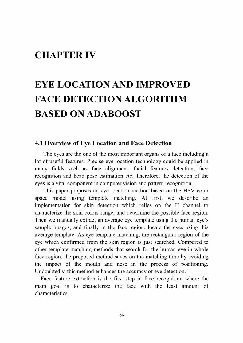
56
CHAPTER IV
EYE LOCATION AND IMPROVED
FACE DETECTION ALGORITHM
BASED ON ADABOOST
4.1 Overview of Eye Location and Face Detection
The eyes are the one of the most important organs of a face including a
lot of useful features. Precise eye location technology could be applied in
many fields such as face alignment, facial features detection, face
recognition and head pose estimation etc. Therefore, the detection of the
eyes is a vital component in computer vision and pattern recognition.
This paper proposes an eye location method based on the HSV color
space model using template matching. At first, we describe an
implementation for skin detection which relies on the H channel to
characterize the skin colors range, and determine the possible face region.
Then we manually extract an average eye template using the human eye’s
sample images, and finally in the face region, locate the eyes using this
average template. As eye template matching, the rectangular region of the
eye which confirmed from the skin region is just searched. Compared to
other template matching methods that search for the human eye in whole
face region, the proposed method saves on the matching time by avoiding
the impact of the mouth and nose in the process of positioning.
Undoubtedly, this method enhances the accuracy of eye detection.
Face feature extraction is the first step in face recognition where the
main goal is to characterize the face with the least amount of
characteristics.

57
At the same time, the characteristics preserve the discriminative ability
among different faces. There are a lot of researches showing how
significant the influence is using different facial feature extraction method
for face recognition. The face region detection should be preceded before
extracting facial features.
4.2 Template Matching and Skin Detection Using HSV Space
First, the RGB image was converted to HSV color space. The skin in
channel H is characterized by values between 0 and 50. After some tests we
proposed to use the channel H with values ranging between 0 and 20
according to our database. Fig.15 shows the same image converted from
RGB to HSV color space. Fig.16 is an intermediary image, where all pixels
classified as skin were set to value 255, and non-skin pixels was fixed to 0.
In the Fig.16 there are many noises, in the classification of pixels like
skin and non-skin. Next step minimizes the effects of the noise pixels using
a 5x5 median filter. Finally, only skin regions are represented as white
pixels. The result is shown in Fig. 17. The binary image aims to retain the
most useful part of image. In many cases, this is a necessary preprocess
before image analysis, feature extraction and pattern recognition.
Fig. 15 Same Image in HSV. Fig. 16 An Intermediary. Fig. 17 The Result of Skin
Detection.
4.2.1 Eye Template Matching
In this paper, the eye template is constructed as follows:
First five images are selected from the face database. They have same
size; then median filter to eliminate the noise and hologram equalization to
reduce the side-effect of illumination are applied to the images. Finally the
same size left and right eyes are obtained manually from the processed
image, the synthetic eye template is determined by the average of left and

58
right eyes respectively. Then the synthetic eye template is created. The final
eye template is shown as Fig.18.
Fig. 18 Left and Right Synthetic Eye Templates.
OpenCV has functions to perform template matching with several
methods depends on the method parameter. It slides through original image,
compares the overlapped patches of size w×h against template using the
specified method and stores the comparison results. Here are the formulas
for the different comparison methods. I denotes image, T is template and R
is result. The summation is done over template and the image patch:
x’=0…w-1, y’ =0…h-1.
Method 1 = CV_TM_SQDIFF
yx
yyxxIyxTyxR,
2)],(),([),(
(4.1)
Method 2 =CV_TM_SQDIFF_NORMED
yx yx
yx
yyxxIyxT
yyxxIyxTyxR
, ,
22
,
2
),(),(
)),(),((),(
(4.2)
Method 3 = CV_TM_CCORR
yx
yyxxIyxTyxR,
)),(),((),(
(4.3)
Method 4 = CV_TM_CCORR_NORMED
yx yx
yx
yyxxIyxT
yyxxIyxTyxR
, ,
22
,
),(),(
)),(),((),(
(4.4)

59
Method 5 = CV_TM_CCOEFF
yx
yyxxIyxTyxR,
)],(),([),(
(4.5)
Where
yxyxThw
yxTyxT
,),()(
1),(),(
yxyxThw
yyxxIyyxxI
,),()(
1),(),(
Method 6 = CV_TM_CCOEFF_NORMED
yx yx
yx
yyxxIyxT
yyxxIyxTyxR
, ,
22
,
),(),(
)),(),((),(
(4.6)
After the function finishes the comparison, the best matches can be
found as global minimums (CV_TM_SQDIFF) or maximums (CV_TM_
CCORR and CV_TM_CCOEFF) using the MinMaxLoc function. In the
case of a color image, template summation in the numerator and each sum
in the denominator are done over all of the channels. In this paper,
experimental results are better when using the method 1.
4.2.2 Face Region Normalization
Fig.19 shows the result of the eye region recognition. Firstly, the range
of eye location can be reduced to the first part of the rectangular area in
according to the distributed character of face region, as eye template
matching, the rectangular face region is just searched; the premise is
accurate detection of the face region. The matching efficiency and error are
both improved.
Fig. 19 Rectangular of Eye Region.
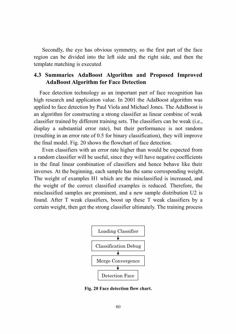
60
Secondly, the eye has obvious symmetry, so the first part of the face
region can be divided into the left side and the right side, and then the
template matching is executed
4.3 Summaries AdaBoost Algorithm and Proposed Improved
AdaBoost Algorithm for Face Detection
Face detection technology as an important part of face recognition has
high research and application value. In 2001 the AdaBoost algorithm was
applied to face detection by Paul Viola and Michael Jones. The AdaBoost is
an algorithm for constructing a strong classifier as linear combine of weak
classifier trained by different training sets. The classifiers can be weak (i.e.,
display a substantial error rate), but their performance is not random
(resulting in an error rate of 0.5 for binary classification), they will improve
the final model. Fig. 20 shows the flowchart of face detection.
Even classifiers with an error rate higher than would be expected from
a random classifier will be useful, since they will have negative coefficients
in the final linear combination of classifiers and hence behave like their
inverses. At the beginning, each sample has the same corresponding weight.
The weight of examples H1 which are the misclassified is increased, and
the weight of the correct classified examples is reduced. Therefore, the
misclassified samples are prominent, and a new sample distribution U2 is
found. After T weak classifiers, boost up these T weak classifiers by a
certain weight, then get the strong classifier ultimately. The training process
Fig. 20 Face detection flow chart.
Loading Classifier
Classification Debug
Merge Convergence
Detection Face
Region

61
is divided into three steps: first extract the Haar characteristics; then
convert the Haar characteristics into the corresponding weak classifiers;
Finally choose the optimal weak classifier from a large number of weak
classifiers. In this section, an improved training algorithm for AdaBoost is
proposed to bring down the complexity of human face detection. Two
methods are adopted to accelerate the training: (1) A method to solve the
parameters of a single weaker classifier is proposed, making the training
speed is higher than probability method; (2) a double threshold decision for
a single weaker classifier is introduced, and the number of weaker classifier
in the AdaBoost system is reduced. Based on the simplified detector, both
the training time and the detecting time could be reduced.
4.4 Experiments and Results
4.4.1 Eye Location Experimental Results
In this section, we will present the experimental results of our algorithm.
Binary images converted from original color images are shown in Fig. 21.
We conducted experiments using 50 images without spectacles for
testing. The success rate of proposed method is 96%. Fig. 22 shows
example of the image for which the proposed method could correctly detect
the both eyes. The eyes are mainly located in the half of upper face region.
Fig. 21 Some Examples for Binary Faces without Spectacles.

62
Fig. 22 Results of eye detection without Spectacles.
The searching process is applied in the upper half of the face region.
This could avoid the error matching among eyes, mouth and nose. The
following results show that the proposed method could correctly locate the
eye part, regardless of the facial expression.
There are some error recognitions, as Fig. 25. And it doesn’t have good
performance for the faces with spectacles.
Fig. 23 Some Results of Eye Location with Expressionless Images.
Fig. 24 Results of Expressive Images, the Original Images of These Examples
Expressing Various Expressions.

63
Fig. 25 Error Recognition Examples.
Fig. 26 Detection results using AdaBoost.
4.4.2 Face Detection Experimental Results
The experimental results show that the proposed algorithm obtained
more accurate testing results, and it can simplify the system structure which
reduced the training time, speed up about 1.5 times. Furthermore the
proposed algorithm has multi-resolution analysis ability. Fig. 26 shows
some face detection results.
One of the fundamental techniques that enable such natural human
computer interaction is face detection. Face detection is the step stone to all
facial analysis algorithms, including face alignment, face modeling, face
relighting, face recognition, head pose tracking, facial expression
tracking/recognition, gender/age recognition, and many more.
We use the Ren-FEdb video database [TK06] collected from 2005 to
2008 including 1,728 videos taken for 96 persons. One has 6 different kind
of expression and each expression is to test. The training set should be
chosen representatively and attempt to include different expression
variation.

64
CHAPTER V
PRIMARILY STUDIED WAVELET
BASED FEATURE EXTRACTION AND
SUPPORT VECTOR MACHINES
5.1 Wavelet Transform Analysis Method
Wavelet transform method is an increasingly popular tool in image
processing and computer vision. Wavelet transform has nice features of
space frequency localization and mustier solutions. The main reasons for
Wavelet transforms lie in its complete theoretical framework, the great
flexibility for choosing bases and the low computational complexity.
Wavelets decompose complex signals into sums of basic functions in this
respect they are similar to other discrete image transforms. Not only there
two big classes of wavelet transform continuous and discrete - but discrete
transform can be redundant, or orthogonal. Each category contains
innumerable possibilities, Daubechies wavelets alone constituting a very
big class.
5.1.1 Formal Definition of Wavelet Transform
The wavelet transform is similar to the Fourier transform (or much
more to the windowed Fourier transform) with a completely different merit
function. The main difference is this: Fourier transform decomposes the
signal into sins and cosines, i.e. the functions localized in Fourier space; in
contrary the wavelet transform uses functions that are localized in both the
real and Fourier space. Generally, the wavelet transform can be expressed
by the following equation:

65
(5.1)
where the * is the complex conjugate symbol and function ψ is some
function. This function can be chosen arbitrarily provided that obeys
certain rules.
As it is seen, the Wavelet transform is in fact an infinite set of various
transforms, depending on the merit function used for its computation. This
is the main reason, why we can hear the term “wavelet transforms” in very
different situations and applications. There are also many ways how to sort
the types of the wavelet transforms. Here we show only the division based
on the wavelet orthogonally. We can use orthogonal wavelets for discrete
wavelet transform development and non-orthogonal wavelets for
continuous wavelet transform development. These two transforms have the
following properties:
(1) The discrete wavelet transform returns a data vector of the same length
as the input is. Usually, even in this vector many data are almost zero. This
corresponds to the fact that it decomposes into a set of wavelets (functions)
that are orthogonal to its translations and scaling. Therefore we decompose
such a signal to a same or lower number of the wavelet coefficient
spectrum as is the number of signal data points. Such a wavelet spectrum is
very good for signal processing and compression, for example, as we get
no redundant information here.
(2) The continuous wavelet transform in contrary returns an array one
dimension larger than the input data. For a 1D data we obtain an image of
the time-frequency plane. We can easily see the signal frequencies
evolution during the duration of the signal and compare the spectrum with
other signals spectra. As here is used the non-orthogonal set of wavelets,
data are correlated highly, so big redundancy is seen here. This helps to see
the results in a more humane form.
5.1.2 Discrete Wavelet Transform
The discrete wavelet transform (DWT) is an implementation of the
wavelet transform using a discrete set of the wavelet scales and translations

66
obeying some defined rules. In other words, this transform decomposes the
signal into mutually orthogonal set of wavelets, which is the main
difference from the continuous wavelet transform (CWT), or its
implementation for the discrete time series sometimes called discrete-time
continuous wavelet transform (DT-CWT).
The wavelet can be constructed from a scaling function which describes
its scaling properties. The restriction that the scaling functions must be
orthogonal to its discrete translations implies some mathematical
conditions on them which are mentioned everywhere, e.g. the dilation
equation
(5.2)
where S is a scaling factor (usually chosen as 2). Moreover, the area
between the function must be normalized and scaling function must be
orthogonal to its integer translations, i.e.
(5.3)
After introducing some more conditions (as the restrictions above does
not produce unique solution) we can obtain results of all these equations,
i.e. the finite set of coefficients ak that define the scaling function and also
the wavelet. The wavelet is obtained from the scaling function as N where
N is an even integer. The set of wavelets then forms an orthonormal basis
which we use to decompose the signal. Note that usually only few of the
coefficients ak are nonzero, which simplifies the calculations.
In the following figure, some wavelet scaling functions and wavelets
are plotted. The most known family of orthonormal wavelets is the family
of Daubechies. Her wavelets are usually denominated by the number of
nonzero coefficients ak, so we usually talk about Daubechies 4, Daubechies
6, etc. wavelets. Roughly said, with the increasing number of wavelet
coefficients the functions become smoother. See the comparison of
wavelets Daubechies 4 and 20 below. Another mentioned wavelet is the
simplest one, the Haar wavelet, which uses a box function as the scaling
function.
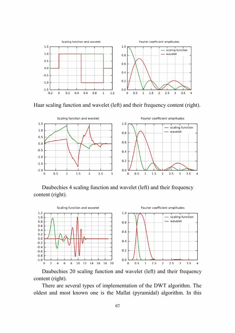
67
Haar scaling function and wavelet (left) and their frequency content (right).
Daubechies 4 scaling function and wavelet (left) and their frequency
content (right).
Daubechies 20 scaling function and wavelet (left) and their frequency
content (right).
There are several types of implementation of the DWT algorithm. The
oldest and most known one is the Mallat (pyramidal) algorithm. In this

68
algorithm two filters – smoothing and non-smoothing one – are constructed
from the wavelet coefficients and those filters are recurrently used to obtain
data for all the scales. If the total number of data D = 2N is used and the
signal length is L, first D/2 data at scale L/2N - 1 are computed, then
(D/2)/2 data at scale L/2N - 2, … up to finally obtaining 2 data at scale L/2.
The result of this algorithm is an array of the same length as the input one,
where the data are usually sorted from the largest scales to the smallest
ones.
Within Gwyddion the pyramidal algorithm is used for computing the
discrete wavelet transform. Discrete wavelet transform in 2D can be
accessed using DWT module.
Discrete wavelet transform can be used for easy and fast denoising of a
noisy signal. If we take only a limited number of highest coefficients of the
discrete wavelet transform spectrum, and we perform an inverse transform
(with the same wavelet basis) we can obtain more or less denoised signal.
There are several ways how to choose the coefficients that will be kept.
Within Gwyddion, the universal thresholding, scale adaptive thresholding
and scale and space adaptive thresholding is implemented. For threshold
determination within these methods we first determine the noise variance
guess given by
(5.4)
where Yij corresponds to all the coefficients of the highest scale subband of
the decomposition (where most of the noise is assumed to be present).
Alternatively, the noise variance can be obtained in an independent way,
for example from the AFM signal variance while not scanning. For the
highest frequency subband (universal thresholding) or for each subband
(for scale adaptive thresholding) or for each pixel neighbourhood within
subband (for scale and space adaptive thresholding) the variance is
computed as
(5.5)
Threshold value is finally computed as

69
(5.6)
where
(5.7)
When threshold for given scale is known, we can remove all the
coefficients smaller than threshold value (hard thresholding) or we can
lower the absolute value of these coefficients by threshold value.
5.1.3 Continuous Wavelet Transform
Continuous wavelet transform (CWT) is an implementation of the
wavelet transform using arbitrary scales and almost arbitrary wavelets. The
wavelets used are not orthogonal and the data obtained by this transform
are highly correlated. For the discrete time series we can use this transform
as well, with the limitation that the smallest wavelet translations must be
equal to the data sampling. This is sometimes called Discrete Time
Continuous Wavelet Transform (DT-CWT) and it is the most used way of
computing CWT in real applications.
In principle the continuous wavelet transform works by using directly
the definition of the wavelet transform, i.e. we are computing a convolution
of the signal with the scaled wavelet. For each scale we obtain by this way
an array of the same length N as the signal has. By using M arbitrarily
chosen scales we obtain a field N×M that represents the time-frequency
plane directly. The algorithm used for this computation can be based on a
direct convolution or on a convolution by means of multiplication in
Fourier space.
The choice of the wavelet that is used for time-frequency
decomposition is the most important thing. By this choice we can influence
the time and frequency resolution of the result. We cannot change the main
features of WT by this way (low frequencies have good frequency and bad
time resolution; high frequencies have good time and bad frequency
resolution), but we can somehow increase the total frequency of total time
resolution. This is directly proportional to the width of the used wavelet in
real and Fourier space. If we use the Morlet wavelet for example (real

70
part – damped cosine function) we can expect high frequency resolution as
such a wavelet is very well localized in frequencies. In contrary, using
Derivative of Gaussian (DOG) wavelet will result in good time localization,
but poor one in frequencies.
5.2 Support Vector Machines
SVM is a learning technique that is considered an effective method for
general purpose pattern recognition because of its high generalization
performance without the need to add other knowledge. Intuitively, given a
set of points belonging to two classes, a SVM finds the hyper plane that
separates the largest possible fraction of points of the same class on the
same side, while maximizing the distance from either class to the hyper-
plane. According to, this hyper plane is called Optimal Separating Hyper
plane (OSH) which minimizes the risk of misclassifying not only the
examples in the training set but also the unseen example of the test set.
SVM is suitable for average size face recognition systems because
normally those systems have only a small number of training samples.
The original SVM algorithm was invented by Vladimir N. Vapink and
the current standard incarnation was proposed by Vapnik and Cortes in
1995. The SVM can be used in the pattern recognition and regression
estimation. In recent years, the SVM has become a research focus of
artificial intelligence. It belongs to machine learning, pattern recognition
and artificial neural network, and other disciplines. It has obvious
advantages compared with existing theories and methods: (1) SVM is a
classification algorithm based on the structural risk minimization principle.
It has achieved higher generalization ability using the limited training
samples than other classification algorithms. SVM obtains the small error
on the limited training samples, which could be guaranteed on the
independent test samples; (2) SVM algorithm is a convex optimization
problem, the local optimal solution must be a global optimal solution. In
addition, the scale of the optimization problem is only related to the sample
number, and has nothing to do with the sample dimension. It is very
suitable for solving the problem which has the high dimension and fewer
samples, such as face recognition.
5.2.1 Linear SVM

71
Given some training data D, a set of n points of the form
(5.8)
where the yi is either 1 or −1, indicating the class to which the point xi
belongs. Each xi is a p-dimensional real vector. We want to find the
maximum-margin hyperplane that divides the points having yi =1from
those having yi = -1. Any hyperplane can be written as the set of points x
satisfying
w·x-b = 0 (5.9)
where · denotes the dot product and w the normal vector to the
hyperplane. The parameter determines the offset of the hyperplane
from the origin along the normal vector w.
If the training data are linearly separable, we can select two
hyperplanes in a way that they separate the data and there are no points
between them, and then try to maximize their distance. The region bounded
by them is called "the margin". These hyperplanes can be described by the
equations w·x-b = 1 and w·x-b = -1.
By using geometry, we find the distance between these two hyperplanes
is , so we want to minimize . As we also have to prevent data points
from falling into the margin, we add the following constraint: for each i
either w·xi –b 》1 for xi of the first class or w·xi –b 》1 for xi of the second.
This can be rewritten as:
(5.10)
We can put this together to get the optimization problem:
Minimize (in w,b)

72
Subject to (for any i=1,…,n) .
5.2.2 Nonlinear Classification
The original optimal hyperplane algorithm proposed by Vapnik in 1963
was a linear classifier. However, in 1992, Bernhard E. Boser, Isabelle M.
Guyon and Vladimir N. Vapnik suggested a way to create nonlinear
classifiers by applying the kernel trick (originally proposed by Aizerman et
al.[AM64]) to maximum-margin hyperplanes.[BB92] The resulting
algorithm is formally similar, except that every dot product is replaced by a
nonlinear kernel function. This allows the algorithm to fit the
maximum-margin hyperplane in a transformed feature space. The
transformation may be nonlinear and the transformed space high
dimensional; thus though the classifier is a hyperplane in the
high-dimensional feature space, it may be nonlinear in the original input
space.
If the kernel used is a Gaussian radial basis function, the corresponding
feature space is a Hilbert space of infinite dimensions. Maximum margin
classifiers are well regularized, so the infinite dimensions do not spoil the
results. Some common kernels include:
Polynomial (homogeneous): k(xi,xj) = (xi,xj)d
Polynomial (inhomogeneous): k(xi,xj) = (xi,xj+1)d
Gaussian radial basis function:
for ɤ>0 Sometimes parameterized using
Hyperbolic tangent: k(xi,xj) = tanh (kxi,xj+c), for some (not every)
k>0 and c<0
The kernel is related to the transform by the
equation . The value w is also in the transformed
space, with . Dot products with w for classification can
again be computed by the kernel trick, i.e. .

73
However, there does not in general exist a value w' such that
.
5.3 Proposed Method based on Wavelet Transform Method and
SVM
In this paper, we chose wavelet decomposition to extract facial features,
because wavelet decomposition decomposes the signal into two parts: low
and high frequency L1 and H1. In two level decomposition, the subimage of
low frequency is decomposed into low frequency L2 and high frequency
H2. For two dimensional signals like face images, wavelet decomposition
is not complete after the row transformation and rank transformation.
Wavelet decomposition is not only diminished but the expression variation
also reduced the image size in the low frequency subimage.
5.3.1 Facial Feature Extraction based on Wavelet Transformation
Method
Low frequency subimages of two faces of the same person after wavelet
decomposition. (a) Original images with different facial expression, image
size 64×64. (b) The results of two level wavelet decomposition. (c)
Reconstructed images, image size 16×16.
In summary, this paper proposes the facial feature extraction as follows:
Select the wavelet basis db4 in the Daubechies wavelet and apply
level two wavelet decomposition that is conducted to the standard
face region. Get low frequency subimage I1 and low frequency
subimage I2.
I1 image matrix is arranged into the vector V1 according to the row or
rank order.
Obtain the vector Vh through horizontal direction grayscale integral
projection applied to image H1; the image I1 is divided into two parts:
upper and lower, then seeking the vertical direction grayscale integral
projection of the previous two part images Vv1 and Vv2, and combine
Vh, Vv1 and Vv2 into another vector V2.

74
Fig. 27 Examples of facial images for two-dimensional wavelet de-
composition with depth 2.
Finally V1 and V2 will be combined into face feature vector, x.
The extracted features from human images by wavelet decomposition are
less sensitive to facial expression variations as shown in Fig.27.
Despite of the low frequency subimage after wavelet decomposition
losing the high frequency component, but it still has the ability of
distinguishing different human faces. The wavelet analysis has obtained
broad application and development in signal process for the
above-mentioned reason.
5.3.2 Classification based on SVM
In support vector machines for classification, the structure of the
complex depends on the number of support vectors, instead of the
characteristic dimension of the space, which is effective to solve the
nonlinear and curse dimensionality problem in machine learning. Fig.28
shows the classification schemes of SVM diagram.
SVM is developed from the theory of linearly separable optimal hyper
plane. The basic idea of the two classes SVM is that first transform the
input sample space into feature space by using non-linear transformation;
then searches the optimum classification hyper plane in this feature space.
This non-linear transformation is obtained by defining the appropriate
kernel function.
The two classes’ samples which are closest to the optimum linearity
classification hyper plane are called SVM. Considering two linearly
separable classes : assume the training data (xi, yi), i = 1, …, l,

75
y
a1y1 a2y2 …… asys
K(x1,x) K(x2,x) K(xs,x)
x1 x2 …… xs
Fig. 28 Classification schemes of SVM.
xi ∈ {+1, -1} can be separated by a hyper plane (w·x) + b = 0 with no
mistake. According to the intuitive speculation, the classification hyper
plane which has the largest distance with two type’s samples will get the
best generalization ability (generation).
Optimal hyper plane is determined by the nearest sample points, and no
relationship with the other samples. You can use the following form to
describe the hyper plane of sample interval: (w·x) + b = 0, ‖w‖= 1, so it is
y = 1, if (w·x) + b ≥ g(x); y = -1, (w·x) + b ≤ g(x).
Input vectors are x = (x1, x2, …, xs), output result is expressed as
y , the weight is wi = aiyi, nonlinear transformation
based on support vectors is x1, x2, …, xs. SVM mainly processes the two
class classify captions problem. Multi-class problem can be processed
through the combination of some two classes support vector machines. The
ordinary methods have one-against-rest, one-against-one and DAGSVM,
etc. In this paper, we use one-against-one algorithm for face recognition.
5.4 Experiments and Results
Table 10 shows the results of the 9/9 experiment. In 9/9 experiment, the
support vector machine misclassified 24 videos only, the recognition rate is
96.78 percent; in 7/11 experiment, the support vector machine misclassified
93 videos, the recognition rate is 94.6 percent.
+

76
Table 10 Comparison Recognition Rates.
Table 11 shows the recognition rate results of the proposed method for
RBF kernel function and other methods. The performance is better than the
references [36], [37] and [38]. The experimental results demonstrate the
effectiveness of the proposed algorithm in this paper. The above
experiments were performed using Emgu CV and C# running on Intel (R)
Core (TM) i7 CPU, 2.80 Ghz. Table I shows the classification experimental
results of two groups. The classification results obtained by three kernel
functions are almost same with better recognition rates as shown in Table
11.
In 9/9 experiment the average classification recognition rate of three
kernel functions is 96.57 percent; in 7/11 experiment the average
classification recognition rate of three kernel functions is 95.65 percent.
Reference [36] extracted the facial features using PCA and classified by
SVM, the recognition rate is 95.15 percent. And in reference[37] were used
Kernel
function RBF Polynomial Linear
Random
testing
number
9/9 7/11 9/9 7/11 9/9 7/11
1 92.8 95.4 95.3 95.7 96.8 96.3
2 97.3 93.9 96.4 97.9 97.0 94.6
3 95.6 93.1 95.8 95.6 96.5 95.0
4 97.6 98.6 96.3 94.8 98.7 94.3
5 96.5 93.6 95.8 96.6 97.0 94.5
6 97.8 96.7 96.2 94.4 98.5 97.8
7 98.5 95.7 94.4 95.6 96.5 96.3
8 96.8 92.8 95.2 96.4 97.0 96.9
9 95.4 92.8 94.3 95.5 95.4 93.7
10 96.8 94.7 94.8 96.8 97.0 94.9
11 97.3 96.7 96.3 96.3 98.0 95.6
12 95.9 93.2 95.4 97.6 97.4 94.5
13 97.3 94.0 97.4 96.5 98.0 96.9
14 96.9 96.3 94.3 95.0 96.0 98.4
15 97.2 93.4 96.8 97.0 94.0. 96.4
16 97.8 91.4 97.7 96.5 98.0 93.2
17 95.6 96.8 95.8 96.0 96.0 97.8
18 97.6 92.2 94.6 96.8 94.2 95.3
19 96.7 94.5 96.8 95.0 97.4 95.8
20 95.8 94.5 93.7 96.0 96.6 94.3
Average 96.78 95.61 94.8 95.13 95.57 94.93

77
for the Gabor + PCA + SVM and Gabor + KPCA + SVM methods
respectively, obtained 93.1 percent and 94.5 percent recognition rates. The
Table 11 Comparison Experimental Results.
proposed method based on RBF kernel function achieved a recognition rate
of 96.78 percent.
A highly accurate and superior face recognition system based on the
wavelet decomposition and SVM technique has been proposed. An
improved AdaBoost algorithm is adopted to detect the face region and
reduce the complexity of human face. The facial features are obtained by
wavelet decomposition, which are less sensitive to the facial expression
variations. SVM is used to classify the human faces.
Extensive experiment shows the validity of the present system in terms
of the parameter at the starting frame shown as Fig.29. SURF is based on
sums of 2D Haar wavelet responses and makes an efficient use of integral
images.
Frame = 5 Frame = 15 Frame = 25
Fig. 29 The Face Detecting and Tracking using SURF Method. (In this system,
capture the video from the second frame, nearer to the second frame, the more
feature points lines)
Methods Recognition Rate
Wavelet+SVM [proposed method] 96.78%
Gabor+SVM [36] 95.15%
Gabor+KPCA+SVM [37] 94.50%
Gabor+PCA+SVM [37] 93.10%
Gabor+rank correlation [38] 91.50%

78
Fig. 30 Automatic Frontal Face Recognition System interface.
Face detection result
Surf method tracking
Recognition results
Same person’s all videos

79
CHAPTER VI
CONCLUSIONS AND FUTURE WORK
6.1 Conclusions
In this paper we have presented an extensive survey of machine
recognition of human faces and a brief review of related studies. We have
considered two face recognition tasks: one is facial feature extraction and
the other is classification. In addition to a detailed review of representative
work, we have provided summaries of current developments and
challenging issues. We have categorized proposed methods of solving these
problems and discussed the pros and cons of these methods. Finally, the
main contribution of this thesis includes:
(1) A novel fast fractal image compression
A novel fast fractal image coding algorithm based on texture feature is
proposed. The most fractal image encoding time is spent on determining
the approximate D-block from a large D-blocks library by using the global
searching method. Clustering the D-blocks library is an effective method to
reduce the encoding time. First, all the D-blocks are clustered into several
parts based on the new texture feature alpha derived from variation
function; second, for each R-block, the approximate D-blocks are searched
for in the same part. In the search process, we import control parameter δ,
this step avoids losing the most approximate D-block for each R-block.
Finally, the R-blocks whose least errors are larger than the threshold given
in advance are coded by the quad tree method. The experimental results
show that the proposed algorithm can be over 6 times faster compared to
the moment-feature-based fractal image algorithm; in addition, proposed
algorithm also improves the quality of the decoded image as well increases
the PSNR’s average value by 2 dB.

80
(2) Provided a thorough survey of the AFR history
The latest AFR survey was published in the year 2000, which in fact
surveyed the AFR researches before 1999. This thesis has provided a more
recent overview of the AFR research and development. Then, AFR
methods are further categorized according to facial feature extraction, face
representation, and classification separately. We also survey the main
public face databases and performance evaluations protocols, based on
which the state-of-the-arts of AFR are summarized. Finally, the challenges
and technical trends in AFR fields are discussed.
(3) Proposed an eye location algorithm based on HSV color space and
template matching
The quality of feature extraction will directly affect recognition results.
Eyes are the one of the most important organs of a face including a lot of
useful features. Therefore, eye location has become one of the most
significant techniques in pattern recognition.
This thesis proposed an eye location method based on the HSV color
space model using template matching. At first, we describe an
implementation for skin detection which relies on the H channel to
characterize the skin colors range, and determine the possible face region.
Then we manually extract an average eye template using the human eye’s
sample images, and finally in the face region, locate the eyes using this
average template. As eye template matching, the rectangular region of the
eye which confirmed from the skin region is just searched. Compared to
other template matching methods that search for the human eye in whole
face region, the proposed method saves on the matching time by avoiding
the impact of the mouth and nose in the process of positioning.
Undoubtedly, this method enhances the accuracy of eye detection.
(4) Investigated the face detection methods, and proposed an improved
training AdaBoost algorithm for face detection
Face detection technology as an important part of face recognition has
high research and application value. In 2001 the AdaBoost algorithm was
applied to face detection by Paul Viola and Michael Jones.

81
In this section, an improved training algorithm for AdaBoost is proposed
to bring down the complexity of human face detection. Two methods are
adopted to accelerate the training: (1) A method to solve the parameters of
a single weaker classifier is proposed, making the training speed is higher
than probability method; (2) a double threshold decision for a single
weaker classifier is introduced, and the number of weaker classifiers in the
AdaBoost system is reduced. Based on the simplified detector, both the
training time and the detecting time could be reduced.
(5) Primarily studied wavelet transform based feature extraction and
Support vector machines to face recognition problem; recognition
rate is analyzed and evaluated experimentally
The extracted features from human images by wavelet decomposition are
less sensitive to facial expression variation. As a classifier, SVM provides
high generation performance without transcendental knowledge. First, we
detect the face region using an improved AdaBoost algorithm. Second, we
extract the appropriate features of the face by wavelet decomposition, and
compose the face feature vectors as input to SVM. Third, we train the SVM
model by the face feature vectors, and then use the trained SVM model to
classify the human face. In the training process, three different kernel
functions are adopted: Radial basis function, Polynomial and Linear kernel
function. Finally, we present a face recognition system that can achieve
high recognition precision and fast recognition speed in practice.
Experimental results indicate that the proposed method can achieve
recognition precision of 96.78 percent based on 96 persons in Ren-FEdb
database that is higher than other approaches.
6.2 Future Work
Face recognition is a challenging problem in the field of image analysis
and computer vision that has received a great deal of attention over the last
few years because of its many applications in various domains. Research
has been conducted vigorously in this area for the past four decades or so,
and though huge progress has been made, encouraging results have been
obtained and current face recognition systems have reached a certain
degree of maturity when operating under constrained conditions; however,

82
they are far from achieving the ideal of being able to perform adequately in
all the various situations that are commonly encountered by applications
utilizing these techniques in practical life. The ultimate goal of researchers
in this area is to enable computers to emulate the human vision system and,
as has been aptly pointed out by Torres [34], “Strong and coordinated effort
between the computer vision, signal processing, and psychophysics and
neurosciences communities is needed” to attain this objective.

83
REFERENCES
[MB04] Mandelbrot, Benoît B. (2004). Fractals and Chaos. Berlin: Springer. p. 38.
ISBN 978-0-387-20158-0. "A fractal set is one for which the fractal
(Hausdorff-Besicovitch) dimension strictly exceeds the topological dimension"
[MB83] Mandelbrot, Benoît B. (1983). The fractal geometry of nature. Macmillan.
ISBN 978-0-7167-1186-5. Retrieved 1 February 2012.
[GJ96] Gouyet, Jean-François (1996). Physics and fractal structures. Paris/New York:
Masson Springer. ISBN 978-0-387-94153-0.
[FK03] Falconer, Kenneth (2003). Fractal Geometry: Mathematical Foundations and
Applications. John Wiley & Sons, Ltd. xxv. ISBN 0-470-84862-6.
[BJ92] Briggs, John (1992). Fractals:The Patterns of Chaos. London, UK: Thames and
Hudson. p. 148. ISBN 0-500-27693-5, 0500276935.
[VT92] Vicsek, Tamás (1992). Fractal growth phenomena. Singapore/New Jersey:
World Scientific. pp. 31; 139–146. ISBN 978-981-02-0668-0.
[HS12] Hu, Shougeng; Cheng, Qiuming; Wang, Le; Xie, Shuyun (2012). "Multifractal
characterization of urban residential land price in space and time". Applied
Geography 34: 161
[FJ89] Feder J. (1989).Fractals.New York, London: Plenum Press.
[MB86] Mandelbrot B.B. (1986).Self-affine fractal sets.In Pietronero L., Tosatti E.
(eds.): Fractals in Physics. Amsterdam: North Holland.
[FY92] Fischer, Yuval (1992-08-12). Przemyslaw Prusinkiewicz, ed. "SIGGRAPH'92
course notes - Fractal Image Compression". [[SIGGRAPH]]. Fractals - From Folk
Art to Hyperreality. ACM SIGGRAPH.
[BW99] Brendt Wohlberg, Gerhard de Jager:"A Review of the Fractal Image Coding
Literature", IEEE Trans.on Image Processing, Vol. 8, No.12,
pp.1716-1729(1999).
[YF95] Y.Fisher: "Fractal image compression theory and application", Spring-Verlag,
New York, pp.1-77(1995).
[HB93] Hurtgen B, Stiller C: " Fast hierarchical codebook search for fractal coding of
still image", EOS/SPIE Visual Communication and PACS for Medical
Application'93, Berlin(1993).
[SY04]Sun Yunda, Zhao Yao, Yuan Baozong: "Region-Based Fractal Image Coding
with Freely-Shaped Partition, Chinese Journal of Electronics", Vol.13, No.3, pp.
506-511(2004).

84
[TY03] Tan Yusong, Zhou Xingming: "A Novel Improved Algorithm of Fractal Image
Compression", ACTA ELECTRONICA SINICA., Vol.31, No.11, pp.
1739-1742(2003).
[SD] Saupe D:"Fractal image compression by multi-dimensional nearest neighbour
search", In: Storer
[CY01] Chen Y, Zhang F:"Feature difference classification method in fractal image
coding", In: Proc IEEE DCC’2001 ,Snowbird ,UT,2001.490
[CZ04] Chen Zuoping, Ye Zhenglin, Gao Xuefeng:"A Fast Fractal Coding Method
Based on Moment Invariant", Computer Engineering and Applications., Vol40,
No.33, pp.62-66(2004).
[YC09] Y.Chakrapani, K.Soundera Rajan:"Implementation of Fractal Image
Compression Employ Hybrid Genetic-Neural Approach", INTERNATIONAL
JOURNAL OF COMPUTATIONAL COGNITION, Vol.7, No.3, pp.33-39,
US(2009-9).
[MF88] M.F.Barnsley:"Fractal modeling of real world images", In: The Science of
Fractal Images, H._O.Peitgen and D.Saupe(eds.), Springer-Verlag, New
York(1988).
[MF86] M.F.Barnsley, V.Ervin, D.Hardin, J.Lancaster: "Solution of an inverse problem
for fractal and other sets", Proceedings of the National Academy of
Science,83(1986).
[AE89] A.E.Jacquin: "A fractal theory of iterated Markov operators with applications to
digital image coding", PhD dissertation, Georgia Institute of Technology,
Intlanta(1989-8).
[AE93] A.E.Jacquin: "Fractal image coding: A review", Proceedings of the IEEE,
Vol.81(1993-10).
[BW99] B. Wohlberg, G. de Jager:" A Review of the Fractal Image Coding Literature",
IEEE Trans.on Image Processing,1999,8(12):1716-1729
[SKM] S.K.Mitra, C.A.Murthy, Malay K.Kundu: "Technique for Fracrtal Image
Compression Using Genetic Algotithm", IEEE Transactions on Image Processing,
Vol.7, No.4, pp.586-593.
[SK98] Suman K.Mitra, C.A.Murthy, Malay K.Kundu:"Technique for Fractal Image
Compression Using Genetic Algorithm", IEEE Transactions on Image
Processing, Vol.7, No.4, pp.586-593(1998).
[MF10] Makoto Fujimural, Hideo Kuroda:"Considerations of Image Compression
Scheme Hiding a Part of Coded Data into Own Image Coded Data", International
Joural of Signal Processing,Image Processing and Pattern Recognition, Vol.3,

85
No.3,pp. 41-48(2010-10).
[CQ10] Changqin Quan and Fuji Ren: A blog emotion corpus for emotional
expression analysis in Chinese, Computer Speech and Language,
Vol.24, No.1, pp.726-749,2010.
[FR09] Fuji Ren: Affective Information Processing and Recognizing Human Emotion,
Electronic Notes in Theoretical Computer Science, Vol.225,No.2009,pp.39-50
[CB65] H,Chan and W.W.Bledsoe, A man-machine facial recognition system: some
preliminary results, Technical report, Panoramic Research Inc., Cal, 1965.
[GH71] A.J.Goldstein, L.D.Harmon and A.B.Lesk. Identification of human faces.
Proceeding of the IEEE, 1971, 59(5):748-760.
[Ka73] T.Kanade. Picture processing system by computer and recognition of human
faces. Ph.D Dissertation. Kyoto University, 1973.
[KB76] Gerald J.Kaufman and Kenneth J.Breeding. The automatic recognition of
human faces from profiles silhouettes. IEEE Transaction on Systems, Man and
Cyhernetics, 6(2), pp113-121, 1976.2.
[HH77] L.Harmon and W.Hunt, Automatic recognition of human face profile,
Computer Graphic and Image Process, vol.6, pp.135-156,1977.
[HK81] L.Harmon, M.K.Khan et al.Machine identification of human faces. Pattern
Recognition, 13(2):97-110.1981.
[Ve98] Thomas Vetter, Synthesis of Novel Views from a Single Face Image, IJCV,
28(2), pp103-116, 1998.
[BR02] Volker Blanz, Sami Romdhani and Thomas Vetter, Face Identification across
different Poses and Illuminations with a 3D Morphale Model, Proceedings of the
IEEE International Conference on Automatic Face and Gesture Recognition,
2002, pp202-207.
[BT03] V.Blanz and T.Vetter Face Recognition Based on Fitting a 3D Morphable
Model, TPAMI, vol 25, no 9, pp 1063-1075, 2003.
[SH97] A.Shasua, On Photometric Issues in 3D visual recognition from a single 2D
Image, International Journal of Computer Vision, 21(1/2),99-122, 1997.
[GB00] A.S.Georghiades, P.N.Behumeur, D.JKriegman, From Few to Many:Generative
Models for Recognition Under Variable Pose and Illumination, Processing of the
4th
International Conference on Face and Gesture Recognition, pp277-284,
Grenoble, France, 2000.3.
[BJ01] R.Basri, D.Jacobs, Lambertian Reflectance and Linear Subspaces, ICCV 2001,
Beckman Institute, Vol.2, p383-390,2001.
[Ra02] R.Ramamoorthi, Analytic PCA construction for theoretical analysis of lighting

86
variability in images of a Lambertial object, IEEE PAMI, 24(10), pp:1322-1333,
Oct 2002.
[table 1] W.ZHAO, R.Chellappa, P.J.Phillips and A.Rosenfeld, Face Recogniton: A
Literature Survey, ACM Computing Surveys, Vol.35, No.4, pp:399-458,
December 2003.
[table 2.3] A.S.Tolba, A.H.El-Baz, and A.A.El-Haeby, Face Recognition: A Literature
Review, International Journal of Information and Communication Engneering,
2:2, pp:88-103, 2006,
[PM00] P.J.Phillips, H.Moon, etc. “The Feret Evaluation Methodology for
Face-Recognition Algorithms”, IEEE Transactions on PAMI, Vol.22, No.10,
pp1090-1104, 2000.
[PG03] P.J.Philips, P.J.Grother, R.J.Micheals,D.M.Blackburn, E.Tabassi and J.M.Bone,
Face Recognition Vendor Test 2002: Evaluation report, Technical Report,
NISTIR 6965, National Institute of Standards and Technology, 2003,
http://www.frvt.org.
[CW95] R.Chellappa, C.L.Wilson, Saad Sirohey, Human and Machine Recognition of
faces: A survey, Proceedings of the IEEE, vol.83, no.5, 1995,5.
[ZCR00] W.Zhao, R.Chellappa, A.Rosenfeld and P.J.Phillips. “ Face Recognition: A
Literature Survey”. CS-Tech Report-4167, University of Maryland, 2000.
[MA94] Y.Moses, Y.Adini and S.Ullman. Face recognition: The problem of
compensating for changes in illumination direction. IN Proc. The Third
European Conference on Computer Vision, 1994.
[AM97] Y.Adini, Y.Moses,S.Ullman, Face Recognition: The Problem of Compensating
for changes in illumination Direction,IEEE Trans,On PAMI,19(7),pp721-732,
1997.
[BV99] Volker Blanz, Thomas Vetter, A Morphable Model For the Synthesis of 3D
Faces, SIG’GRAPH’99, 1999.
[CB65] H.Chan and W.W.Bledsoe, A man-machine facial recognition system: some
preliminary results, Technical report, Panoramic Research Inc., Cal, 1965.
[CB65] H.Chan and W.W.Bledsoe, A man-machine facial recognition system: some
preliminary results, Technical report, Panoramic Research Inc., Cal, 1965.
[GH71] A.J.Goldstein,L.D.Harmon and A.B.Lesk. Identification of human faces,
Proceeding of the IEEE, 1971,59(5):748-760.
[HH77] L.Harmon and W.Hunt, Automatic recognition of human face profile,
Computer Graphic and Image Process, vol.6,pp.135-156, 1977.
[RB98] H.A.Rowley, S.Baluja, and T.Kanade, Neural network-based face detection,

87
IEEE-PAMI,20(1), 23-38,1998.
[GM02] R.Gross, I.Matthews, and S.Baker. Eigen light-fields and face recognition
across pose. Proceedings of the IEEE International Conference on Automatic
Face and Gesture Recognition, May 2002.
[PA96] P.Penev and J.Atick, “Local Feature Analysis: A General Statistical Theory for
Object Representation,” Network: Computation in Neural Systems, vol.7,
pp.477-500, 1996.
[BH96] P.Belhumeur, J.Hespanha and D.Kriegman, Eigenfaces vs. Fisherfaces:
Recognition using class specific linear projection. In Proceedings of Fourth
European Conference on Computer Vision, ECCV’96,pp45~56, 1996.
[BH97] P.N.Bellhumer, J.Hesoanha and D.Kriegman. Eigenfaces vs.fisherfaces:
Recognition using class specific linear projection. IEEE Transactions on Pattern
Analysis and Machine Intelligence, Special Issue on Face Recognition,
17(7):711-720,1997
[BL90] J.Buhmann, M.Lades, von der Malsberg. Size and distortion invariant object
recognition by hierarchical graph matching. In: Proceedings of IEEE Intl. Joint
Conference on Neural Networks, pp.411-416, SanDiego, 1990
[BP93] R.Brunelli, T.Ppggio, Face recognition: features vs. templates.IEEE Trans.on
PAMI,15(10):1042-1052,1993
[BH01] A.U.Batur, M.H.Hayes, Linear subspace for illumination robust face
recognition , Pro.of CVPR01, 2001
[CW1995] R.Chellappa, C.L.Wilson, Saad Siroher, Human and Machine Recognition of
faces:A survey, Proceedings of the IEEE, vol.83,no.5, 1995.5
[CE98] T.F.Cootes, G.J.Edwards, C.J.Taylor, Active Appearance Model,
Proc.European Conf. Computer Vision, vol.2, pp.484-498,1998
[DC01]O.Deniz, M.Castrillon, M.Hernanades, “Face Recognition Using Independernt
Component Analysis and Support Vector Machines”. Int. Conf. on Audio- and
Video-Based person Authentication, Lecture Notes, pp.59-64, 2001
[EC99] G.Edwards, T.Cootes, and C.Taylor, Advances in Active Appearance Models,
Proc. Int’l Conf. Computer Vision, pp.137-142,1999
[GB01] Athinodoros S.Georghiades, Peter N.Belhumeur, David J.Kriegman, From Few
to Many: Illumination Cone Models for Face Recognition Under Variable
Lighting and Pose,IEEE Trans.on PAMI,23(6)pp.125-139, 2001.6
[GK98] A.S.Georghiades, D.J.Kriegman and P.N.Belhumeur, “Illumination Cones For
Recognition Under Variable Lighting:Faces”. Proc.of IEEE CVPR, pp52-58,1998
[GL00] G.Guo,S.Z.Li and K.Chan, “Face Recognition by Support Vector Machines”,

88
Proc.of the 4th
Int.Conf. on Auto. Face and Gesture Recog, pp.196-201, Grenoble,
2000.3
[LV93] M.Lades, J.C.Vorbruggen, J.Buhman, J.Lange, C.V.D.Malshurg, R.P.Wurtz,
W.Konen, Distortion Invariant Object Recognition in the Dynamic Link
Architecture, IEEE Trans. On Computers, 42(3),pp 300-311,1993
[LT94] A.Lanitis, C.J.Taylor and T.F.Cootes. An automatic face identification system
using flexible appearance models, In British Machine Vision Conference, BMVA
Press, 1994,1:6-74
[LT95] A.Lanitis, C.Taylor and T.Cootes , A Unified Approach to Coding and
Interpreting Face Images, Proc.Int’l Conf. Computer Vision, pp.368-373, 1995
[LT97] A.Lanitis, C.Taylor and T.Cootes. Automatic interpretation and coding of face
images using flexible models. IEEE Transactions on Pattern Analysis & Machine
Intelligence , vol.19, no.7,pp.743-756, July,1997
[LH01] K.C.Lee, J.Ho, D.Kriegman, Nine points of Light:Acquiring Subspaces for Face
Recognition under variable lighting, CVPR01
[MP97] B.Moghaddam and A.Pentland, Probabilistic Visual Learning for Object
Representation IEEE trans. ON PAMI, vol.20, no.7,pp696-710,1997
[Ph98] P.J.Phillps, Support vector machines applied to face recognition. In Advances in
Neural Information Processing Systems, page 803. Editors:M.CMozer,M.I.Jordan,
and T. Petsche, MIT Press, 1998
[RB02] Sami Romdhani, Volker Blanz, Thomas Vetter, Face Identification by Fitting a
3D Morphable Model Using Linear Shape and Texture Error Functions,
Proceedings of the 7th
European Conference on Computer Vision, Vol.4, pp3-19,
May, 2002, Editor A.Heyden et al.
[RL00] Sam Roweis &Lawrence Saul.Nonlinear dimensionality reduction by locally
linear embedding. Science, V.290, no.5500,2000, pp. 2323-2326.
[SR01] A.Shashua and T.Riklin-Raviv, “The Quotient Image: Class-Based
Re-Rendering And Recognition With Varying Illumination”, IEEE Trans. On
PAMI, 23(2):pp129-139,2001.2
[SK87] L.Sirovich and M.Kirby, Low-dimensional Procedure for the characterization of
Human Faces.J.Opt.Soc.Am.A, vol4,NO3,519-524,1987
[VJ01] Paul Viola, M.Jones, Rapid Object Detection using a Boosted Cascade of
Simple, CVPR-2001
[VJo01]Paul Viola, M.Jones, Fast and Robust Classification using Asymmetric,
NIPS-2001
[TS00] J.B.Tenenbaum,V.de Silva and J.C.Langford, A Global Geometric Framework

89
for Nonlinear Dimensionality Reduction, Science 290(5500):2319-2323,22
December 2000
[WF97] L.Wiskott, J.M.Fellous, N.Kruger, C.v.d.Malsburg, Face Recognition by
Elastic Bunch Graph Matching, IEEE Trans. On PAMI, vol.19,no.7,pp775-779,
1997
[YK02] Ming-Hsuan Yang, David J.Kriegman, Narendra Ahuja, Detecting Faces in
Images: A Survey, IEEE PAMI,Vol.24, No.1, pp34-58, Jan.2002
[KS90] M.Kirby and L.Sirovich, Application of the Karhunen-Loeve procedure for the
characterization of human faces, IEEE Trans, PAMI, 12(1),103-108,1990
[TP91] M.Turk, A.Pentland. Eigen-faces for Recognition Jounal of cognitive
neuroscience, 3(1),pp71-86,1991
[JM00] K.Jonsson, J.Matas, J.Kittler, Y.P.Li, Learning Support Vectors for Face
Verification and Recognition, Proceeding of the 4th
International Conference on
Face and Gesture Recognition, pp 208-213, Grenoble, France, 200,3[SVM]
[JK02] K.Jonsson, Josef Kittler, YOngping Li, Jiri Matas: Support vector machines for
face authentication. Image and Vision Computing.20(5-6):369-375,(2002)
[PM94] Alex Pentland, Baback Moghaddam, Thad starner. View-Based and Modular
Eigen-space for Face Recognition MIT Media Lab perceptual Computing Section
Tech IEEE Conference on Computer Vision & Pattern Recognition 1994.
[YK02] Ming-Hsuan Yang, David J.Kriegman, Narendra Ahuja, Detecting Faces in
Images: A Survey, IEEE PAMI, vol.24, No.1, pp34-58, Jan.2002.
[ZZ02] Z.Q.Zhang, L.Zhu,S.Z.Li, H.J.Zhang, “Real-Time Multi-view Face Detection”.
In Proceeding of The 5th
International Conference on Automatic Face and Gesture
Recognition, Washington, DC,USA, 20-21, May, 2002
[ZC98] W.Zhao, R.Chellappa, and A.Krishnaswamy, “Discriminant Analysis of
Principal Component for Face Recognition”, Proc.of Inter.Conf.On Auto. Face
and Gesture Recognition, pp.336-341, 1998
[ZC00] W.Zhao, R.Chellappa, SFS Based View Synthesis for Robust Face Recognition,
Proceeding of the 4th
International Conference on Face and Gesture
Recognition,pp285-292, Grenoble, France, 2000.3
[ZG03] Yi Zhou, Lie Gu, HOngjiang Zhang, Bayesian Tangent Shape Model:
Estimating Shape and Pose Parameters via Bayesian Inference, Proceeding of the
IEEE Conference on Computer Vision and Pattern Recognition(CVPR 2003),
Wisconsin, USA, June, 16-22, 2003
[LZ04] Stan Z.Li,Zhen Qiu Zhang, “FloatBoost Learning and Statistical face
detection”,IEEE Transactions on pattern analysis and machine intelligence,
90
accepted , 2004
[Liu99] C.Liu, Statistical and evolutionary approaches for face recognition, George
mason University, Ph,D Dissertation, 1999
[LH02] Q.S.Liu, R.Huang, H.Q.Lu and S.D.Ma, Face recognition using Kernel based
Fisher Discriminant Analysis, Proc. Int’l Conf. Automatic face and gesture
Recognition, pp 197-201,2002
[LW01] C.Liu and H.Wechsler: A Shape and texture based Enhanced Fisher Classifier
for Face recognition, IEEE Trans.Image Processing , vol.10, no.4,
pp.598-608,2001
[LW02] C.Liu and H.Wechsler: Gabor Feature based Classification Using the Enhanced
Fisher Linear Discriminant Model for Face Recognition , IEEE Trans.Image
Processing, vol.11, no.4, pp.467-476,2002
[LW03] C.Liu and H.Wechsler: Independent Component Ananysis of Gabor Features
fro Face Recognition. IEEE Trans. Neural network, vol.14, no.4,pp.919-928,
2003
[LL99] S.Li and J.Lu. face recognition using nearest feature line , IEEE Trans.Neural
Network, vol.10, no.2, pp.439-443,1999
[LO95] J.Lampinen and E.Oja. Distortion tolerant pattern recognition based on
self-organizing feature extraction.IEEE Transactions on Neural networks,
6(3):539-547,1995
[LG97] Steve Lawrence . Lee Giles, Ah Chung Tsoi, Andrew D.Back, Face
Recognition: A Convolutional Neural-Networl Approach,IEEE Trans. On Neural
Network, vol.8, No.1, Jun. 1997
[LW99] C.J.Liu and H.Wechsler, “Comparative Assessment of Independent Component
Analysis(ICA) for face recognition”, Int. Conf.on Audio and Video Based
Biometri Person Authentication, 1999
[LY99] Janhuang Lai, P.C.Yuen, G.C.Feng, Spectroface: A Fourier-based Approaches
for Human Face Recognition,ICMI, Vol.2, 115-120,1999
[LC93] K.Liu, Y.Cheng, J.Yang. Algrbraic feature extraction for image recognition
based on an optimal discriminant criterion.Pattern Recognition,
26(6):903-911,1993
[LT94] A.Lanitis, C.J.Taylor and T.F.Cootes. An automatic face identification system
using flexible appearance models . In British Machine Vision Conference,
BMVA Press, 1994, 1:65-74
[Lee96] T.S.Lee, Image Representation Using 2d Gabor Wavelets.IEEE Trans.Pattern
Analysis and Machine Intelligence , 18(10):959-971, 1996

91
[LY01] JIan huang Lai, P.C.Yuen, G.C.Feng, face recognition using Holistic Fourier
Invariant features, Pattern Recognition , 34(1), 95-109,2001
[LY02] S.Z.Li,S.C.Yan,H.J.Zhang,Q.S.Cheng, Multi-view face alignment using direct
appearance models, Proceedings of the 5th
international conference on
Automatic face gesture recognition , pp324-329, Washington, DC,USA, 20-21,
May, 2002
[Ne99] A.Nefian, “A Hidden Markon Model-Based Approach for Face Detection and
Recognition”, Ph.D.Thesis, Georgia Institute of Technology, 1999
[MP95] B.Moghaddam and A.Pentland, Probalilistic Visual Learning for Object
Detection, Proc. Int’l Computer Vision , pp.786-793,1995
[MP00] Baback Moghaddam, Tony Jebara, Alex PEntland, Bayesian Face Recognition,
Pattern Recognition Vol.33(2000),pp1771-1782,2000
[Mo02] B.Moghaddam, Principal Manifolds and probalilistic subspace for visual
recognition,IEEE Trans. PAMI 24(6)780-788,2002
[MC92] B.S.Manjunath, R.Chellappa, C.V.Malsburg, A Feature based approach to face
recognition, in Pro.IEEE Computer Soc.Con.On Computer Vision and pattern
recognition, 1992, pp373-378
[PL92] S.J.Perantonis and P.J.G.Lisboa, “Translation, rotation, and scale invariant
pattern recognition by high-order neural networks and moment classifiers”, IEEE
Trans, Neural Networks, vol.3, pp.241-251,Mar1992
[Sa93] F.Samaria, face segmentation for identification using Hidden Markov Models,
Proceeding of the 4th
British Machine Vision Conference,Springer-Verlag. 1993
[Sa94] F.Samaria. Face Recognition Using Hidden Markov Models. PhD thesis, Trinity
College, University of Cambridge, Cambridge, 1994.
[SG03] S.Shan, W.Gao, D.Zhao, Face Identification Based On Face-Specific Subspace,
International Journal of Image and System Technology, 13(1), pp23-32, 2003
[SR01] A.Shashua and T.Riklin-Raviv, “The Quotient Image: Class-Based
Re-Rendering And Recognition With Varying Illuminations”, IEEE Trans. on
PAMI, 23(2): pp129-139, 2001.2
[SGW03] Shiguang Shan, We n Gao, Wei Wang, Debin Zhao, Baocai Yin. Enhanced
Active Shape Models with Global Texture Constraints for Face Image Analysis,
Fourteenth International Symposium On Methodologies For Intelligent Systems,
N.Zhong et al. (Eds.): ISMIS 2003, LNAI2871, pp593-597, Springer, Maebashi
City, Japan, Oct.2003
[ST00] M.B.Stegmann, Active Appearance Models, Theory, Extension and Cases,
Master thesis, Technical University of Denmark, 2000

92
[SY94] F.Samaria, & S.Young, HMM-based architecture for face identification
International Vision Conference, 12(8), 537-543. 1994
[Xs94] X.Xie, R.Sudhakar, H.Zhuang, Improving eye feature-extraction using
deformable templates. Pattern Recognition, 27(6), 791-799, 1994
[TK01] A.Tefas, C.Kotropoulos, and I.Pitas, Using Support Vector Machines to
Enhance the Performance of Elastic Graph Matching for Frontal Face
Authentication, IEEE Transactions On Pattern Analysis And Machine
Intelligence, VOL. 23, NO. 7, pp735-746, JULY 2001
[TT03] Y.Tian, T.Tan and Y.Wang, Do Singular Values Contains Adequate
Information for Face Recognition? Pattern Recognition, Vol. 36, No.3,
pp.649-655, 2003.
[KT00] C.L.Kotropoulos, A.Tefas, I.Pitas. Frontal Face Authentication Using
Discriminating Grids with Morphological Feature Vectors, IEEE trans. On
Multimedia, Vol.2, No.1, pp14-26 March, 2000
[Kr00] V. Krueger. Gabor wavelet networks for object representation. . DAGM
Symposium, Kiel, Germany, 9, 13-15, 2000.
[KW88] M.Kass, A.Witkin, and D.Terzopoulos. Snakes: Active contour models. Int.
Journal of Computer Vision, pp.321-331,1988
[WT04] X. Wang, and X. Tang, "A Unified Framework for Subspace Face
Recognition," To appear in IEEE Transactions on Pattern Analysis and Machine
Intelligence (PAMI), 2004.
[WL04] Haitao Wang, Stan Z. Li, and Yangsheng Wang. "Generalized Quotient Image".
In Proceedings of IEEE International Conference on Computer Vision and Pattern
Recognition. Washington, DC. 27th June - 2nd July, 2004.
[WA03] Tong Wang, Haizhou Ai, Gaofeng Huang, A Two-Stage Approach to
Automatic Face Alignment, Proceedings of SPIE - The International Society for
Optical Engineering, v5286, n2, 2003, p558-563
[YA00] M.H.Yang, N. Ahuja, D. Kriegman Face Recognition Using Kernel Eigenfaces,
Int. Conf. on Image Processing, 2000, vol. 1, pp. 37-40
[Ya02] M.H.Yang. “Kernel Eigenfaces vs Kernel Fisherfaces: Face Recognition Using
Kernel Methods”. Proc. Int’l. Conf. Automatic Face and Gesture Recognition,
pp.215-210, 2002.
[YY01] H. Yu aand J. Yang, “A Direct LDA Algorithm for High-dimensional Data –
with Application to Face Recognition”. Pattern Recognition , Vol. 34, pp
2067-2070, 2001.
[Yu91] A.L.Yuille, Deformable templates for face detection, J. Cogn. neurosci. 3, 59-70,

93
1991.
[YH92] A.L.Yuille, P.W.Hallinan, D.S.Cohen, Feature extraction from faces using
deformable templates. International Journal of Computer Vision, 8, 99-111. 1992
[YL03] S.C. Yan, C. Liu, S.Z. Li. H.J. Zhang, H. Shum, Q.S. Cheng. "Face Alignment
Using Texture-Constrained Active Shape Models". Image and Vision Computing.
Pages 69-75. Vol.21, Issue 1 , 10 January 2003.
[Ho91] Z.Hong. Algebraic feature extraction of image for recognition. Pattern
Recognition, 24(3),pp:211-
219, 1991
[HL01] X.W. Hou, S.Z. Li, H.J. Zhang, Q.S. Cheng. "Direct Appearance Models". In
Proceedings of IEEE International Conference on Computer Vision and Pattern
Recognition. Hawaii. December, 2001.
[CL00] L.F.Chen, H.M.Liao, J.C.Lin, M.T.Ko, and G.J.Yu. “A New LDA-based Face
Recognition System Which Can Solve the Small Sample Size Problem”. Pattern
Recognition, vol. 33, no.10, pp. 1713-1726, 2000.
[CW02] Jen-Tzung Chien, Chia-Chen Wu, Discriminant Waveletfaces and Nearest
Feature Classifiers for Face Recognition, IEEE Transactions On Pattern Analysis
And Machine Intelligence, VOL. 24, NO. 12, pp1644-1649, DECEMBER 2002
[CT95] T. F. Cootes, C. J. Taylor, D. H. Cooper and J. Graham, Active Shape Models –
Their Training and Application., Computer Vision and Image Understanding, Vol.
61, No. 1, January, pp. 38-59, 1995.
[CL93] G.Chow, X.B.Li Towards a system for automatic facial feature detection.
Pattern Recognition, 26(12), pp1739-1755. 1993
[CW00] T.F.Cootes, K.Walker, C.J.Taylor, View-based Active Appearance Models,
Proceeding of the 4th International Conference on Face and Gesture Recognition,
pp227-232, Grenoble, France, 2000.3
[BL98] M.S.Bartlett, H.M.Lades and T.J.Sejnowski. “Independent Component
Representations for Face Recognition”. Proc. of SPIE, 2399, pp.528-539, 1998.
[Be95] David Beymer, Vectorizing Face Images by Interleaving Shape and Texture
Computation, A.I.Memo No. 1537, 1995.9
[BH96] P.Belhumeur, J.Hespanha, and D.Kriegman, Eigenfaces vs. Fisherfaces:
Recognition using class specific linear projection. in Proceedings of Fourth
European Conference on Computer Vision, ECCV’96, pp45~56, 1996
[BP92] R. Brunelli and T. Poggio, Face Recognition through Geometrical Features,
Proceedings of ECCV '92, pp792-800
[SH94] F. S. Samaria, and A. C. Harter. Parameterisation of a Stochastic Model for

94
Human Face Identification. Proceedings of the 2nd IEEE Workshop on
Applications of Computer Vision, December 1994.
[SB03] Terence Sim, Simon Baker, and Maan Bsat. The CMU Pose, Illumination and
Expression Database. IEEE Transactions on Pattern Analysis and Machine
Intelligence, VOL. 25, No. 12, December 2003, pp. 1615 – 1618
[MM99] K.Messer, J.Matas, J.Kittler, J.Kittler, J.Luettin, and G.Maitre. XM2VTSDB:
The extended M2VTS database. In Second International Conference on Audio
and Video-based Biometric Person Authentication, March, 1999
[MB98] A.R.Martinez and R.Benavente. The AR face database: Technical Report 24,
Computer Vision Venter (CVC) Technical Report, Barcelona, Spain, June 1998.
[DG01] Hyoja-Dong, and Nam-Gu. Asian Face Image Database PF01. Pohang
University of Science and Technology.
[HB03] B.-W. Hwang, H. Byun, M.-C. Roh, and S.-W. Lee. Performance evaluation of
face recognition algorithms on the asian face database, KFDB. In Audio- and
Video-Based Biometric Person uthentication (AVBPA), pages 557–565, 2003.
[GC04] Wen Gao, Bo Cao, Shiguang Shan, Delong Zhou, Xiaohua Zhang, Debin Zhao.
The CAS-PEAL Large-Scale Chinese Face Database and Evaluation Protocols.
Technical Report No. L_TR_04_FR_001, Joint Research & Development
Laboratory, CAS, 2004. http://www.jdl.ac.cn
[AM64] Aizerman, Mark A.; Braverman, Emmanuel M.; and Rozonoer, Lev I. (1964).
"Theoretical foundations of the potential function method in pattern recognition
learning". Automation and Remote Control 25: 821–837.
[BB92] Boser, Bernhard E.; Guyon, Isabelle M.; and Vapnik, Vladimir N.; A training
algorithm for optimal margin classifiers. In Haussler, David (editor); 5th Annual
ACM Workshop on COLT, pages 144–152, Pittsburgh, PA, 1992. ACM Press.
[KT06] Kuroda, T., Ma J., Ren,F.: The Construction of The Facial Expression Video
Database. Communication Technology, ICCT’06, pp: 1265-1268. International
Conference on Guilin, China, 2006.