Embed Size (px)
Citation preview
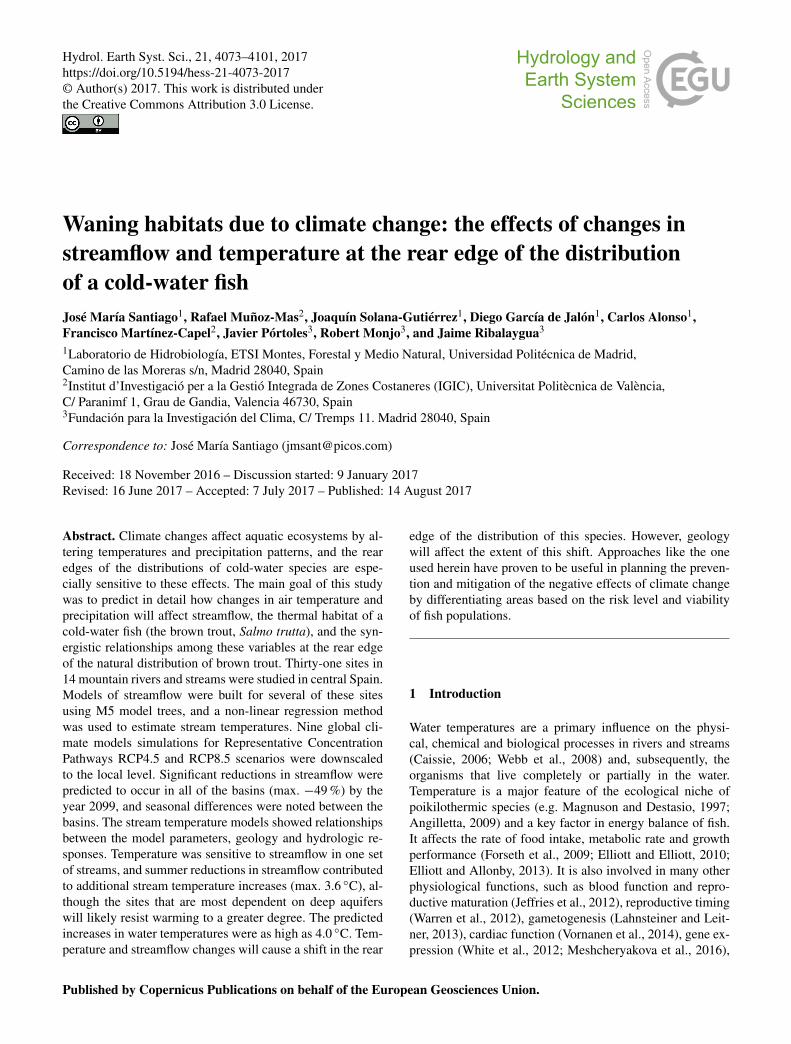
Hydrol. Earth Syst. Sci., 21, 4073–4101, 2017https://doi.org/10.5194/hess-21-4073-2017© Author(s) 2017. This work is distributed underthe Creative Commons Attribution 3.0 License.
Waning habitats due to climate change: the effects of changes instreamflow and temperature at the rear edge of the distributionof a cold-water fishJosé María Santiago1, Rafael Muñoz-Mas2, Joaquín Solana-Gutiérrez1, Diego García de Jalón1, Carlos Alonso1,Francisco Martínez-Capel2, Javier Pórtoles3, Robert Monjo3, and Jaime Ribalaygua3
1Laboratorio de Hidrobiología, ETSI Montes, Forestal y Medio Natural, Universidad Politécnica de Madrid,Camino de las Moreras s/n, Madrid 28040, Spain2Institut d’Investigació per a la Gestió Integrada de Zones Costaneres (IGIC), Universitat Politècnica de València,C/ Paranimf 1, Grau de Gandia, Valencia 46730, Spain3Fundación para la Investigación del Clima, C/ Tremps 11. Madrid 28040, Spain
Correspondence to: José María Santiago ([email protected])
Received: 18 November 2016 – Discussion started: 9 January 2017Revised: 16 June 2017 – Accepted: 7 July 2017 – Published: 14 August 2017
Abstract. Climate changes affect aquatic ecosystems by al-tering temperatures and precipitation patterns, and the rearedges of the distributions of cold-water species are espe-cially sensitive to these effects. The main goal of this studywas to predict in detail how changes in air temperature andprecipitation will affect streamflow, the thermal habitat of acold-water fish (the brown trout, Salmo trutta), and the syn-ergistic relationships among these variables at the rear edgeof the natural distribution of brown trout. Thirty-one sites in14 mountain rivers and streams were studied in central Spain.Models of streamflow were built for several of these sitesusing M5 model trees, and a non-linear regression methodwas used to estimate stream temperatures. Nine global cli-mate models simulations for Representative ConcentrationPathways RCP4.5 and RCP8.5 scenarios were downscaledto the local level. Significant reductions in streamflow werepredicted to occur in all of the basins (max. −49 %) by theyear 2099, and seasonal differences were noted between thebasins. The stream temperature models showed relationshipsbetween the model parameters, geology and hydrologic re-sponses. Temperature was sensitive to streamflow in one setof streams, and summer reductions in streamflow contributedto additional stream temperature increases (max. 3.6 ◦C), al-though the sites that are most dependent on deep aquiferswill likely resist warming to a greater degree. The predictedincreases in water temperatures were as high as 4.0 ◦C. Tem-perature and streamflow changes will cause a shift in the rear
edge of the distribution of this species. However, geologywill affect the extent of this shift. Approaches like the oneused herein have proven to be useful in planning the preven-tion and mitigation of the negative effects of climate changeby differentiating areas based on the risk level and viabilityof fish populations.
1 Introduction
Water temperatures are a primary influence on the physi-cal, chemical and biological processes in rivers and streams(Caissie, 2006; Webb et al., 2008) and, subsequently, theorganisms that live completely or partially in the water.Temperature is a major feature of the ecological niche ofpoikilothermic species (e.g. Magnuson and Destasio, 1997;Angilletta, 2009) and a key factor in energy balance of fish.It affects the rate of food intake, metabolic rate and growthperformance (Forseth et al., 2009; Elliott and Elliott, 2010;Elliott and Allonby, 2013). It is also involved in many otherphysiological functions, such as blood function and repro-ductive maturation (Jeffries et al., 2012), reproductive timing(Warren et al., 2012), gametogenesis (Lahnsteiner and Leit-ner, 2013), cardiac function (Vornanen et al., 2014), gene ex-pression (White et al., 2012; Meshcheryakova et al., 2016),
Published by Copernicus Publications on behalf of the European Geosciences Union.
4074 J. M. Santiago et al.: Waning habitats due to climate change
ecological relationships (Hein et al., 2013; Fey and Herren,2014), and fish behaviour (Colchen et al., 2017).
Natural patterns of water temperature and streamflow areprofoundly linked with climatic variables (Caissie, 2006;Webb et al., 2008). Therefore, stream temperature is stronglycorrelated with air temperature (Mohseni and Stefan, 1999),whereas streamflow has a complex relationship with precip-itation (McCuen, 1998; Gordon et al., 2004). In addition, at-mospheric temperature influences the type of precipitation(rain or snow) that occurs and the occurrence of snowmelt;conversely, river discharge is also a main explanatory factorof water temperature for some river systems (Neumann etal., 2003; van Vliet et al., 2011). Furthermore, geology af-fects surface water temperatures by means of groundwaterdischarge (Caissie, 2006; Loinaz et al., 2013), influenced bythe aquifer depth (shallow or deep) and the water’s residencetime (Kurylyk et al., 2013; Snyder et al., 2015).
Climate change is already affecting aquatic ecosystemsby altering water temperatures and precipitation patterns.Stream temperature increases have been documented overthe last several decades over the whole globe, such as inEurope (e.g. Orr et al., 2015, documented a mean increasein stream temperature of 0.03 ◦C per year in England andWales), Asia (e.g. Chen et al., 2016, documented a meanincrease in stream temperature of 0.029–0.046 ◦C per yearin the Yongan River, eastern China), America (e.g. Kaushalet al., 2010, documented mean increases in stream tempera-ture of 0.009–0.077 ◦C per year) and Australia (e.g. Chess-man, 2009, documented mean increases in stream temper-ature of 0.12 ◦C per year between macroinvertebrate sam-pling campaigns). Abundant information is also available re-garding the impact of recent climate changes on streamflowregimes worldwide (e.g. Luce and Holden, 2009; Leppi etal., 2012) and, more specifically, in the Iberian Peninsula(e.g. Ceballos-Barbancho et al., 2008; Lorenzo-Lacruz et al.,2012; Morán-Tejeda et al., 2014). However, detailed predic-tions are uncommon (e.g. Thodsen, 2007). The predictionsof the Intergovernmental Panel on Climate Change (IPCC,2013) suggest that these alterations will continue through-out the 21st century, and they will have consequences for thedistribution of freshwater fish (e.g. Comte et al., 2013; Ruiz-Navarro et al., 2016). These changes may have an especiallystrong effect on cold-water fish, which have been shownto be very sensitive to climate warming (Williams et al.,2015; Santiago et al., 2016). For example, among salmonids,DeWeber and Wagner (2015) found stream temperature to bethe most important determinant of the probability of occur-rence of brook trout, Salvelinus fontinalis (Mitchill, 1814).
The rear edge populations (sensu Hampe and Petit, 2005:“populations residing at the current low-latitude margins ofspecies’ distribution ranges”) of a cold-water species are es-pecially sensitive to changes in water temperature, in ad-dition to reductions in the available habitable volume (i.e.streamflow). The rear edge is the eroding margin of the rangewhere lineages mix, the genetic drift and local adaptations
increase, and droughts put populations under stress. The im-pact of water temperatures on the distribution of salmonidfish is well documented (e.g. Beer and Anderson, 2013; Ebyet al., 2014); however, the combined effects of rising streamtemperatures and reductions in streamflow remain relativelyunexamined, with some exceptions (e.g. Wenger et al., 2011;Muñoz-Mas et al., 2016). Jonsson and Jonsson (2009) pre-dicted that the expected effects of climate change on watertemperatures and streamflow will have implications for themigration, ontogeny, growth and life-history traits of Atlanticsalmon, Salmo salar Linnaeus, 1758, and brown trout, Salmotrutta Linnaeus, 1758. Thus, investigation of these habitatvariables in the context of several climate scenarios shouldhelp scientists to assess the magnitude of these changes onthe suitable range and life history of these species.
The objective of this study is to predict how and to whatextent the availability of suitable habitat for the brown trout,a sensitive cold-water species, will change within its currentnatural distribution under the new climate scenarios througha study of changes in streamflow and temperature and theirinteractions. Specifically, in this paper, we (i) assessed the ef-fects of both streamflow and geology on stream temperature;(ii) predicted the changes in streamflow and stream tempera-ture implied by the climate change scenarios used in the 5thAssessment Report (AR5) of the IPCC; and (iii) assessed theexpected effects of these changes on trout habitat aptitude. Tothis end, hydrologic simulations with M5 model trees cou-pled with non-linear water temperature models at the dailytime step were fed with high-resolution, downscaled versionsof the air temperature and precipitation fields predicted usingthe most recent climate change scenarios (IPCC, 2013). Theeffects of basin geology on the stream temperature modelsand on the estimated changes in thermal regimes were stud-ied. Finally, the changes in the thermal habitat of trout wereassessed by studying the violation of the tolerable tempera-ture thresholds of the brown trout.
2 Materials and methods
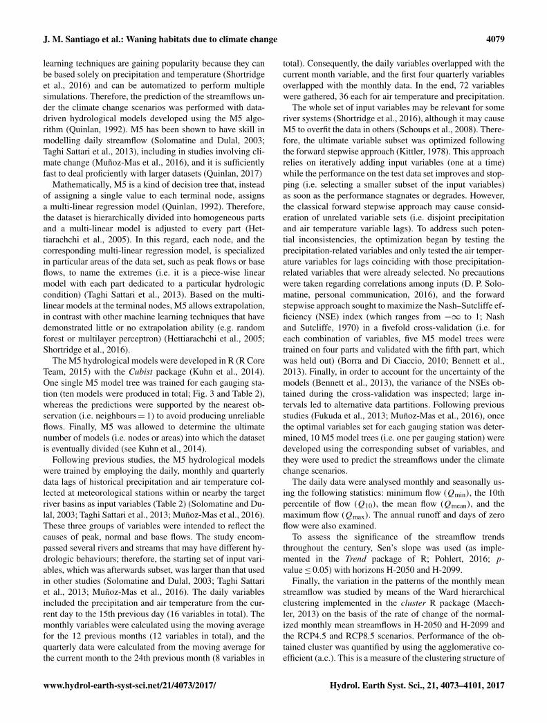
The logical framework followed is summarized in Fig. 1.First, the daily global climate models output presented by theIPCC were downscaled to the study area. Then, the obtainedlocal climate models output were applied to generate simu-lations of streamflow and water temperature. The results aredaily values that can be used for the assessment of fish habitatsuitability and availability.
The procedure yielded results in the form of continuoustime series, but they are presented for two time horizons: theyear 2050 (H-2050) and the year 2099 (H-2099). The valuesfor these horizons correspond to the average of the values ofthe different variables for the decades 2041–2050 and 2090–2099, respectively.
Hydrol. Earth Syst. Sci., 21, 4073–4101, 2017 www.hydrol-earth-syst-sci.net/21/4073/2017/

J. M. Santiago et al.: Waning habitats due to climate change 4075
CMIP5 models + downscaling(Local climate change models)
Air temperaturePrecipitation
Flow model
Stream temperature modelDaily flows
Daily water temperatures
• Hydrological resources• Water quality
• Aquatic communities• Fish habitat
Predicted data
Models
Results
Streamflow Precipitation Air temperature
Stream & air temperatures
O b ser v ed data
Ecologicalthresholds
Fish distrib ution
Figure 1. Logical framework of the study.
Figure 2. River network and location of the study sites (water temperature data loggers), with details regarding lithology. The grid depictsthe actual occurrence of brown trout in Spain.
2.1 Study sites
In total, 31 sites in 14 mountain rivers and streams inhab-ited by brown trout were chosen with the aim of encompass-ing a diverse array of geological and hydrological conditionsin the centre of Spain (between the latitudes of 39◦53′ and41◦21′ N). Specifically, the investigated sites are located inthe Tormes River and its tributaries, the Barbellido River, theGredos Gorge and the Aravalle River (in the Duero Basin);the Cega River and the Pirón River (the Pirón River is a trib-utary of the Cega River in the larger Duero Basin); the Lo-zoya River, the Tagus River, the Gallo River, and the Cabril-las River (all four of which are in the Tagus Basin); theEbrón River and the Vallanca River (the Vallanca River isa tributary of the Ebrón River in the Turia Basin); and thePalancia River and the Villahermosa River (Fig. 2). The ma-
jor geological components that lithologically characterize themountain sites in the Duero and Lozoya basins are igneousrocks; the altitudinally lower sites in the Duero Basin are un-derlain by Cenozoic detrital material, and the eastern basins(Tagus, Gallo, Cabrillas, Ebrón, Vallanca, Palancia and Vil-lahermosa) are underlain primarily by Mesozoic carbonates.The distribution of geological materials was retrieved fromthe Lithological Map of Spain (IGME, 2015) (Table 1).
The land cover type is mainly pine forest in all of thestudied basins (Pinus sylvestris, P. nigra, P. pinea and P.pinaster) (CORINE Land Cover 2006; European Environ-mental Agency, 2007). Only the lower basins of the down-stream sites on the Cega and Pirón rivers are mosaics offorest and croplands, whereas the uppermost sites withinthe Tormes River basin (Barbellido and Gredos Gorge) lieabove the current tree line. Territorial planning does not con-
www.hydrol-earth-syst-sci.net/21/4073/2017/ Hydrol. Earth Syst. Sci., 21, 4073–4101, 2017
4076 J. M. Santiago et al.: Waning habitats due to climate change
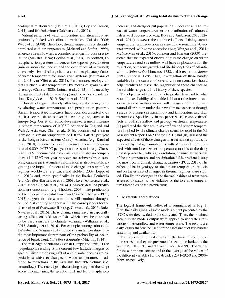
Table 1. Description of the data logger (thermograph) sites, specifying given name, UTM coordinates (Europe WGS89), altitude (metresabove sea level), code of the nearest temperature meteorological station with suitable time series for this study (AEMET: Spanish Meteoro-logical Agency), orthogonal distance between the data logger and the meteorological station, number of recorded days for stream temperatureand characteristic geological nature (lithology) of the data logger site (the last of which was obtained from IGME, 2015). Bold letters indicatesites associated with the gauging stations.
Sites UTM-X UTM-Y Altitude AEMET Distance to AEMET Recording Lithology(m a.s.l.) code station (km) days
Aravalle 283623 4468847 1010 2440 76.4 1257 IgneousBarbellido 311759 4465519 1440 2440 52.2 881 IgneousGredos Gorge 306363 4468087 1280 2440 55.7 644 IgneousTormes1 308751 4469371 1270 2440 53.0 421 IgneousTormes2 297543 4467191 1135 2440 64.0 537 IgneousTormes3 285481 4470750 995 2440 74.1 588 IgneousCega1 427627 4539806 1600 2516 84.5 544 IgneousCega2 429416 4541728 1384 2516 85.8 544 IgneousCega3 428892 4549370 1043 2516 83.9 544 IgneousCega4 426932 4559076 943 2516 81.2 407 Quaternary detritalCega5 408504 4569772 853 2516 63.4 544 Quaternary detritalCega6 389014 4581160 766 2516 47.9 501 Quaternary detritalPirón1 422082 4536456 1475 2516 80.1 544 IgneousPirón2 420660 4537094 1348 2516 78.6 483 IgneousPirón3 409935 4549473 908 2516 65.2 544 Quaternary detritalPirón4 394462 4556823 826 2516 48.9 544 Quaternary detritalPirón5 388615 4560166 815 2516 42.9 424 Quaternary detritalLozoya1 422060 4520319 1452 3104 7.3 2151 IgneousLozoya2 425445 4522314 1267 3104 4.6 1870 IgneousLozoya3 425657 4527327 1142 3104 0.7 1776 IgneousLozoya4 430740 4530050 1090 3104 6.4 2187 IgneousTagus-Peralejos 590887 4494165 1149 3013 27.9 964 CarbonateTagus-Poveda 582900 4502160 1028 3013 22.8 669 CarbonateGallo 583771 4519743 998 3013 10.9 1019 CarbonateCabrillas 585619 4502986 1075 3013 20.8 1070 CarbonateEbrón 643551 4445027 879 8381B 9.5 592 CarbonateVallanca1 644966 4435479 745 8381B 1.8 836 CarbonateVallanca2 645936 4435715 718 8381B 0.8 836 CarbonatePalancia1 694348 4421176 760 8434A 10.4 334 CarbonatePalancia2 697451 4419477 660 8434A 7.8 334 CarbonateVillahermosa 722594 4449436 592 8478 13.5 334 Carbonate
sider significant changes in land use at mid-century; objec-tively, changes are not expected after that time because ahigh percentage of the territory is protected. The studiedreaches are not effectively regulated (only small weirs or nat-ural obstacles exist). One large dam lies on the Pirón River(the Torrecaballeros Dam, which has a capacity of 0.32 hm3
and a maximum depth of 26 m and lies at an altitude of1390 m a.s.l.), but it does not significantly alter the temporalpattern of streamflow (Santiago et al., 2013). In the LozoyaRiver, a large dam (the Pinilla Dam, which has a capacity of38.1 hm3 and a maximum depth of 30 m and lies at an al-titude of 1060 m a.s.l.) exists that separates fish populationsabove and below the reservoir, although it lies downstreamof the studied reach.
Hydrological data characterize the streamflow regimesas extreme winter/early spring (groups 13 and 14 in the
classification of Haines et al., 1988). However, the hydro-graphs show a west-to-east smoothing gradient (Fig. 3). Thissmoothing is associated with the carbonate rocks, whereasgreater seasonality is associated with the igneous and detritalgeological materials.
2.2 Data collection
At each study site, water temperatures were recorded every2 h throughout the year using 31 Hobo® Water Tempera-ture Pro v2 (Onset®) and Vemco® Minilog data loggers lo-cated at several sites along the studied rivers and streams (Ta-ble 1). Loggers were tested for malfunctions before beingdeployed, and they were placed in areas not exposed to di-rect sunshine (Stamp et al., 2014). Meteorological data wereobtained from nine thermometric and 15 pluviometric sta-
Hydrol. Earth Syst. Sci., 21, 4073–4101, 2017 www.hydrol-earth-syst-sci.net/21/4073/2017/

J. M. Santiago et al.: Waning habitats due to climate change 4077
Figure 3. River regime patterns for the different gauging stations. The flows are expressed as percentages of the mean annual flow, and themonths (horizontal axis) are ordered from January to December.
tions of the Spanish Meteorological Agency (AEMET) net-work, and data from 10 gauging stations (from the officialnetwork of the Spanish Water Administration) were obtainedto model the streamflows. The AEMET thermometric sta-tions that lie closest to the stream temperature monitoringsites and have at least 30 years of data between 1955 andthe present were selected. The selected pluviometric stationswere those located within the upstream river basin or nearthe corresponding gauging station (Table 2). The air temper-ature and precipitation data from AEMET were tested to as-sess their reliability by applying a homogeneity test. This testis based on a two-sample Kolmogorov–Smirnov test, and itmarks years as possibly containing inhomogeneous data. Inthe second phase, the marked years are matched against thedistribution of the entire series to determine if they containtrue inhomogeneities, searching for possible dissimilaritiesbetween the empirical distribution functions. Only reliableseries were used. The locations of the stations did not changein the studied period.
2.3 Climate change modelling and downscaling
Data from nine global climate models associated with the 5thCoupled Model Intercomparison Project (CMIP5) were used,namely BCC-CSM1-1, CanESM2, CNRM-CM5, GFDL-ESM2 M, HADGEM2-CC, MIROC-ESM-CHEM, MPI-ESM-MR, MRI-CGCM3, and NorESM1-M (Santiago et al.,2016). These models provided daily data to simulate futureclimate changes corresponding to the Representative Con-centration Pathways RCP4.5 (a stable scenario) and RCP8.5(a scenario including a pronounced increase in CO2 concen-
trations) established in Taylor et al. (2009) and used in theAR5 of the IPCC (2013). An array of nine general climatemodels was used to avoid biases due to the particular as-sumptions and features of each particular model (Kurylyk etal., 2013). Historical simulations of the 20th century wereused to control the quality of the procedure and to comparethe magnitudes of the predicted changes.
Pourmokhtarian et al. (2016) note the importance of theuse of fine downscaling techniques. Thus, a two-step ana-logue statistical method (Ribalaygua et al., 2013) was used todownscale the daily climatic data, specifically the maximumand minimum air temperatures and the precipitation for eachstation and for each day. For both air temperature and precip-itation, the procedure begins with an analogue stratification(Zorita and von Storch, 1999) in which the n days most sim-ilar to each problem day to be downscaled are selected usingfour different meteorological large-scale fields as predictors,specifically (1) the speed and (2) direction of the geostrophicwind at 1000 hPa, as well as (3) the speed and (4) direc-tion of the geostrophic wind at 500 hPa. In a second step,the temperature determination was obtained through multi-ple linear regression analysis using the selected n of the mostanalogous days. This was performed for the maximum andminimum air temperatures at each station and for each prob-lem day. The linear regression uses forward and backwardstepwise selections of the predictors to select only the rel-evant predictive variables for that particular case. For pre-cipitation, a group of m problem days (the whole days of amonth were used) were downscaled together, and the “pre-liminary precipitation quantity”, or the average precipitationof the n most analogous days, was obtained for each prob-
www.hydrol-earth-syst-sci.net/21/4073/2017/ Hydrol. Earth Syst. Sci., 21, 4073–4101, 2017

4078 J. M. Santiago et al.: Waning habitats due to climate change
Table 2. Official stations used (meteorological and hydrological), variables, length of time series used and geographical position. AEMET:Spanish Meteorological Agency; CHD: Water Administration of Duero Basin; CHT: Water Administration of Tagus Basin; and CHJ: WaterAdministration of Júcar Basin.
Institution Code Name Variable Series length used UTM-X UTM-Y Altitude
AEMET 2180 Matabuena pluviometry 1955–2013 436266 4549752 1154AEMET 2186 Turégano pluviometry 1955–2013 415346 4556596 935AEMET 2196 Torreiglesias pluviometry 1970–2013 413294 4550606 1053AEMET 2199 Cantimpalos pluviometry 1955–2013 402524 4547811 906AEMET 2440 Aldea del Rey Niño temperature 1955–2012 356059 4493201 1160AEMET 2462 Puerto de Navacerrada temperature and 1967–2012 414745 4516276 1894
pluviometryAEMET 2516 Ataquines temperature 1970–2013 345716 4560666 802AEMET 2813 Navacepeda de Tormes pluviometry 1965–2012 308892 4470347 1340AEMET 2828 El Barco de Ávila temperature and 1955–1983 285643 4470512 1007
pluviometryAEMET 3009E Orihuela del Tremedal pluviometry 1986–2000 614383 4489759 1450AEMET 3010 Ródenas pluviometry 1968–2006 625505 4499963 1370AEMET 3013 Molina de Aragón temperature and 1951–2010 594513 4521786 1056
pluviometryAEMET 3015 Corduente pluviometry 1961–2000 584125 4523281 1120AEMET 3018E Aragoncillo pluviometry 1968–2010 580519 4531876 1263AEMET 3104 Rascafría-El Paular temperature and 1967–2012 425165 4526895 1159
pluviometryAEMET 8376B Jabaloyas pluviometry 1993–2006 635600 4456215 1430AEMET 8381B Ademuz-Agro temperature and 1989–2010 646722 4436034 740
pluviometryAEMET 8434A Viver temperature 1971–2006 704704 4422256 562AEMET 8478 Arañuel temperature 1971–2006 714943 4438277 406CHD 2006 Tormes-Hoyos del Espino flow 1955–2012 314676 4467908 1377CHD 2016 Cega-Pajares de Pedraza flow 1955–2013 428296 4557678 938CHD 2057 Pirón-Villovela de Pirón flow 1972–2013 405596 4551929 869CHD 2085 Tormes-El Barco de Ávila flow 1955–2012 285173 4470362 992CHD 2714 Cega-Lastras de Cuéllar flow 2004–2013 403509 4571682 838CHT 3001 Tagus-Peralejos de las Truchas flow 1946–2010 590474 4494474 1143CHT 3002 Lozoya-Rascafría (El Paular) flow 1967–2013 425321 4522069 1270CHT 3030 Gallo-Ventosa flow 1946–2010 587349 4520522 1016CHT 3268 Cabrillas-Taravilla flow 1982–2010 587480 4503395 1107CHJ 8104 Ebrón-Los Santos flow 1989–2010 645963 4441366 750
lem day. Thus, the m problem days from the highest to thelowest “preliminary precipitation amount” could be sorted.To assign the final amount of precipitation, each precipita-tion amount of the m× n analogous days was taken. Then,those m× n amounts of precipitation were sorted, and thenthose amounts were clustered into m groups. Every quantitywas then assigned in order to the m days previously sortedby the “preliminary precipitation amount”. Further details ofthe methodology are described in Ribalaygua et al. (2013).
A systematic error is obtained when comparing the simu-lated data from the climate models with the observed data.Such errors are inherently associated with all downscalingmethodologies and climate models, which usually introducebias into their outputs. To eliminate this systematic error,the future climate projections were corrected according toa parametric quantile–quantile method (Monjo et al., 2014),
which was performed by comparing the observed and sim-ulated empirical cumulative distribution functions (ECDFs)and linking them using ECDFs obtained from the down-scaled European Centre for Medium-Range Weather Fore-casts ERA-40 reanalysis daily data (Uppala et al., 2005).
As a result, for each climate change scenario, the dailymaximum and minimum air temperatures (which were usedto infer the mean air temperature) and precipitation were ob-tained for each climate model, and the whole dataset wereused as inputs to simulate the runoff and water temperaturesunder these climate change scenarios.
2.4 Hydrological modelling
Although process-based physical models are considered thestandard hydrological models, flexible data-driven machine
Hydrol. Earth Syst. Sci., 21, 4073–4101, 2017 www.hydrol-earth-syst-sci.net/21/4073/2017/
J. M. Santiago et al.: Waning habitats due to climate change 4079
learning techniques are gaining popularity because they canbe based solely on precipitation and temperature (Shortridgeet al., 2016) and can be automatized to perform multiplesimulations. Therefore, the prediction of the streamflows un-der the climate change scenarios was performed with data-driven hydrological models developed using the M5 algo-rithm (Quinlan, 1992). M5 has been shown to have skill inmodelling daily streamflow (Solomatine and Dulal, 2003;Taghi Sattari et al., 2013), including in studies involving cli-mate change (Muñoz-Mas et al., 2016), and it is sufficientlyfast to deal proficiently with larger datasets (Quinlan, 2017)
Mathematically, M5 is a kind of decision tree that, insteadof assigning a single value to each terminal node, assignsa multi-linear regression model (Quinlan, 1992). Therefore,the dataset is hierarchically divided into homogeneous partsand a multi-linear model is adjusted to every part (Het-tiarachchi et al., 2005). In this regard, each node, and thecorresponding multi-linear regression model, is specializedin particular areas of the data set, such as peak flows or baseflows, to name the extremes (i.e. it is a piece-wise linearmodel with each part dedicated to a particular hydrologiccondition) (Taghi Sattari et al., 2013). Based on the multi-linear models at the terminal nodes, M5 allows extrapolation,in contrast with other machine learning techniques that havedemonstrated little or no extrapolation ability (e.g. randomforest or multilayer perceptron) (Hettiarachchi et al., 2005;Shortridge et al., 2016).
The M5 hydrological models were developed in R (R CoreTeam, 2015) with the Cubist package (Kuhn et al., 2014).One single M5 model tree was trained for each gauging sta-tion (ten models were produced in total; Fig. 3 and Table 2),whereas the predictions were supported by the nearest ob-servation (i.e. neighbours= 1) to avoid producing unreliableflows. Finally, M5 was allowed to determine the ultimatenumber of models (i.e. nodes or areas) into which the datasetis eventually divided (see Kuhn et al., 2014).
Following previous studies, the M5 hydrological modelswere trained by employing the daily, monthly and quarterlydata lags of historical precipitation and air temperature col-lected at meteorological stations within or nearby the targetriver basins as input variables (Table 2) (Solomatine and Du-lal, 2003; Taghi Sattari et al., 2013; Muñoz-Mas et al., 2016).These three groups of variables were intended to reflect thecauses of peak, normal and base flows. The study encom-passed several rivers and streams that may have different hy-drologic behaviours; therefore, the starting set of input vari-ables, which was afterwards subset, was larger than that usedin other studies (Solomatine and Dulal, 2003; Taghi Sattariet al., 2013; Muñoz-Mas et al., 2016). The daily variablesincluded the precipitation and air temperature from the cur-rent day to the 15th previous day (16 variables in total). Themonthly variables were calculated using the moving averagefor the 12 previous months (12 variables in total), and thequarterly data were calculated from the moving average forthe current month to the 24th previous month (8 variables in
total). Consequently, the daily variables overlapped with thecurrent month variable, and the first four quarterly variablesoverlapped with the monthly data. In the end, 72 variableswere gathered, 36 each for air temperature and precipitation.
The whole set of input variables may be relevant for someriver systems (Shortridge et al., 2016), although it may causeM5 to overfit the data in others (Schoups et al., 2008). There-fore, the ultimate variable subset was optimized followingthe forward stepwise approach (Kittler, 1978). This approachrelies on iteratively adding input variables (one at a time)while the performance on the test data set improves and stop-ping (i.e. selecting a smaller subset of the input variables)as soon as the performance stagnates or degrades. However,the classical forward stepwise approach may cause consid-eration of unrelated variable sets (i.e. disjoint precipitationand air temperature variable lags). To address such poten-tial inconsistencies, the optimization began by testing theprecipitation-related variables and only tested the air temper-ature variables for lags coinciding with those precipitation-related variables that were already selected. No precautionswere taken regarding correlations among inputs (D. P. Solo-matine, personal communication, 2016), and the forwardstepwise approach sought to maximize the Nash–Sutcliffe ef-ficiency (NSE) index (which ranges from −∞ to 1; Nashand Sutcliffe, 1970) in a fivefold cross-validation (i.e. foreach combination of variables, five M5 model trees weretrained on four parts and validated with the fifth part, whichwas held out) (Borra and Di Ciaccio, 2010; Bennett et al.,2013). Finally, in order to account for the uncertainty of themodels (Bennett et al., 2013), the variance of the NSEs ob-tained during the cross-validation was inspected; large in-tervals led to alternative data partitions. Following previousstudies (Fukuda et al., 2013; Muñoz-Mas et al., 2016), oncethe optimal variables set for each gauging station was deter-mined, 10 M5 model trees (i.e. one per gauging station) weredeveloped using the corresponding subset of variables, andthey were used to predict the streamflows under the climatechange scenarios.
The daily data were analysed monthly and seasonally us-ing the following statistics: minimum flow (Qmin), the 10thpercentile of flow (Q10), the mean flow (Qmean), and themaximum flow (Qmax). The annual runoff and days of zeroflow were also examined.
To assess the significance of the streamflow trendsthroughout the century, Sen’s slope was used (as imple-mented in the Trend package of R; Pohlert, 2016; p-value≤ 0.05) with horizons H-2050 and H-2099.
Finally, the variation in the patterns of the monthly meanstreamflow was studied by means of the Ward hierarchicalclustering implemented in the cluster R package (Maech-ler, 2013) on the basis of the rate of change of the normal-ized monthly mean streamflows in H-2050 and H-2099 andthe RCP4.5 and RCP8.5 scenarios. Performance of the ob-tained cluster was quantified by using the agglomerative co-efficient (a.c.). This is a measure of the clustering structure of
www.hydrol-earth-syst-sci.net/21/4073/2017/ Hydrol. Earth Syst. Sci., 21, 4073–4101, 2017
4080 J. M. Santiago et al.: Waning habitats due to climate change
the dataset, as expressed by Kaufman and Rousseeuw (2005)and its value ranges between 0 (maximum dissimilarity) and1 (minimum dissimilarity).
2.5 Stream temperature modelling
Stream temperature (Ts) at each thermal sampling site wassimulated from air temperature (Ta) by means of a modi-fied version of the bounded non-linear regression model de-scribed by Mohseni et al. (1998). A previous modification(Term 1 in Eq. 1; Santiago et al., 2016) served to improvethe behaviour of the former model, permitting it to be usedfor daily inputs. In this study, the effect of the instream flow(Q) effect is incorporated. Thus, this model addresses dailymean stream temperature (DMST; Ts in Eq. 1) using the dailymean air temperature (DMAT, Ta in Eq. 1), the 1-day beforevariation in the daily mean air temperature (1Ta in Eq. 1),and the daily mean flow (Qmean, Q in Eq. 1) as predictors.DMST was used because it better reflects the average condi-tions that fish (particularly trout) will experience for an ex-tended period of time (Santiago et al., 2016), and it averagesover daily fluctuations in the radiation and heat fluxes. Themodel is formulated as follows:
Ts = µ+α−µ
1+ eγ (β−Ta)+ λ(1Ta)︸ ︷︷ ︸
Term 1
+ω
1+ eδ(τ−Q)︸ ︷︷ ︸Term 2
, (1)
where µ is the minimum stream temperature (◦C), α is themaximum stream temperature (◦C), β represents the air tem-perature at which the rate of change of the stream tempera-ture with respect to the air temperature is a maximum (◦C),γ (◦C−1) is the value of the rate of change at β, and λ isa coefficient (dimensionless) that represents the resistanceof DMST to change with respect to the 1-day variation inDMAT (1Ta). In the flow component (Term 2 in Eq. 1),ω is the maximum observable variation in stream tempera-ture due to the flow difference (given in ◦C), τ represents theflow value at which the rate of change of the stream temper-ature with respect to the flow is a maximum (m3 s−1), and δ(m−3 s) is this maximum rate at τ . Negative values of λ aredue to the resistance to stream temperature changes, and thusthey must be subtracted from the expected temperature: themore resistant the stream is to temperature change, the closerλ will be to zero. The less resistant the stream is to change,the more negative λ is. The parameter µ was allowed to beless than zero in the modelling process, even though this isthe freezing temperature. Thus, the function would truncateat the freezing point. The relationship between the thermalamplitude α−µ and the indicator of thermal stability λ wasstudied using the Pearson correlation.
A blockwise non-parametric bootstrap regression (Liu andSingh, 1992) was used to estimate the parameters of boththe modified Mohseni models (with and without streamflow),and residual normality and non-autocorrelation were checkedwith the Shapiro test and Durbin–Watson test. Moreover, the
7-day lag PACF (partial autocorrelation function) was ob-tained. These calculations were performed using R. A 95 %confidence interval was calculated for each parameter. Per-formance was quantified using two indicators: the residualstandard error (RSE) and the Nash–Sutcliffe efficiency in-dex (NSE). The Bayesian information criterion (BIC) andthe Akaike information criterion (AIC) were used to test theeight-parameter models (Terms 1 and 2 of Eq. 1) against thefive-parameter models (Term 1 of Eq. 1).
This model can be classified as semi-physically based. Ithas some advantages over machine learning methods, suchas classification and regression trees (De’ath and Fabricius,2000) or random forests (Breiman, 2001), because the modelparameters imply a mechanistic interpretation of how pro-cess drivers act, yielding a higher transferability (Wenger andOlden, 2012). These features make of this model an advanta-geous option for our goals.
2.6 Effects of geology on stream temperature
Geology determines the residence time of deep groundwaterin the aquifers underlying streams (Chilton, 1996), and resi-dence times influence discharge temperatures. To explore therelationships between thermal regimes and geology, a strati-fied study of both the geology classes of the parameter val-ues was completed by means of a t test with the Bonferronicorrection (p-value < 0.05). In the same sense, increments ofthe annual averages of the daily mean (1Tmean), minimum(1Tmin) and maximum (1Tmax) stream temperatures werecalculated and studied by lithological classes (Table 1).
The variation in the patterns of the monthly mean streamtemperature was studied by means of cluster analysis of thetemperature increases corresponding to H-2050 and H-2099for the RCP4.5 and RCP8.5 scenarios (using Ward’s hier-archical clustering as implemented in the cluster package ofR; Maechler, 2013). As said above, agglomerative coefficient(a.c.) was used as a performance indicator.
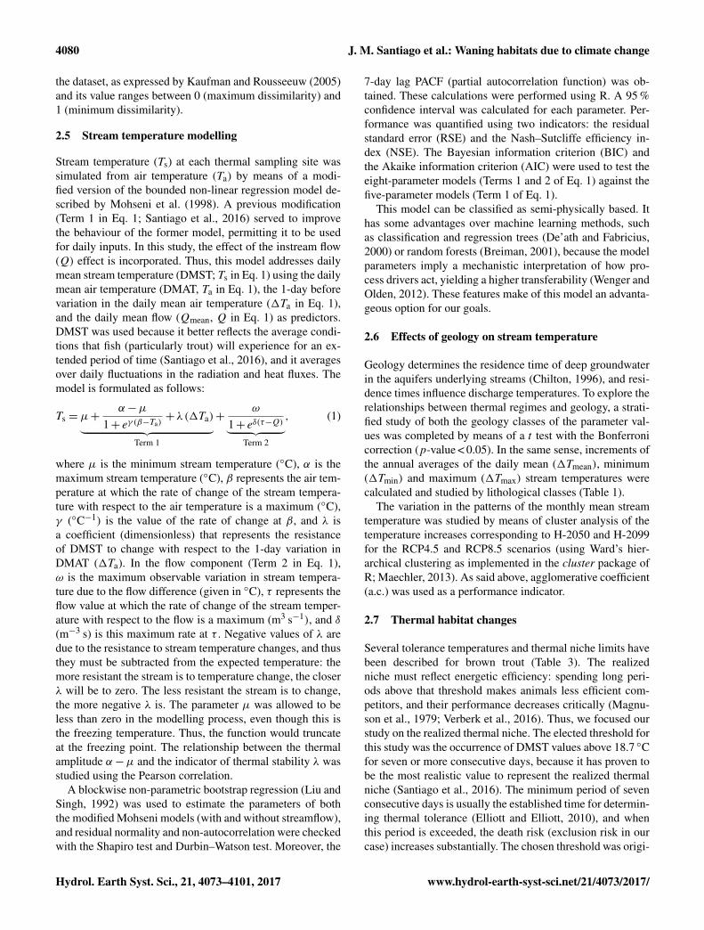
2.7 Thermal habitat changes
Several tolerance temperatures and thermal niche limits havebeen described for brown trout (Table 3). The realizedniche must reflect energetic efficiency: spending long peri-ods above that threshold makes animals less efficient com-petitors, and their performance decreases critically (Magnu-son et al., 1979; Verberk et al., 2016). Thus, we focused ourstudy on the realized thermal niche. The elected threshold forthis study was the occurrence of DMST values above 18.7 ◦Cfor seven or more consecutive days, because it has proven tobe the most realistic value to represent the realized thermalniche (Santiago et al., 2016). The minimum period of sevenconsecutive days is usually the established time for determin-ing thermal tolerance (Elliott and Elliott, 2010), and whenthis period is exceeded, the death risk (exclusion risk in ourcase) increases substantially. The chosen threshold was origi-
Hydrol. Earth Syst. Sci., 21, 4073–4101, 2017 www.hydrol-earth-syst-sci.net/21/4073/2017/
J. M. Santiago et al.: Waning habitats due to climate change 4081
Table 3. Different classes of thermal thresholds for emerged trout classes found in the literature. The type of experiment differentiates theexperiments with controlled (laboratory) and uncontrolled (wild) temperature. Latitude of the experiments’ location is shown.
Variable Temperature) Type of Latitude Reference(◦C experiment
maximum growth 13.1 laboratory 54◦ N Elliott et al. (1995)Maximum growth 16 laboratory 61◦ N Forseth and Jonsson (1994)Maximum growth 16.9 laboratory 43◦ N Ojanguren et al. (2001)Maximum growth 13.2 wild 43◦ N Lobón-Cerviá and Rincón (1998)Maximum growth 13 wild 41◦ S Allen (1985)Maximum growth 15.4–19.1 laboratory 59◦ N Forseth et al. (2009)Thermal optimum 14.2 wild 47◦ N Hari et al. (2006)Upper growth limit 19.5 wild 41◦ S Allen (1985)Upper thermal niche 20 wild 47◦ N Hari et al. (2006)Upper thermal niche∗ 18.1 wild 41◦ N Santiago et al. (2016)Upper thermal niche∗ 18.7 wild 41◦ N Santiago et al. (2016)Critical feeding temperature 19.4 laboratory 54◦ N Elliott et al. (1995)Critical feeding temperature ≥ 23 laboratory 59◦ N Forseth et al. (2009)Incipient lethal temperature∗ 24.7 laboratory 54◦ N Elliott (1981)Ultimate 27.8 laboratory 60◦ N Grande and Andersen (1991)Ultimate∗∗ 29.7 laboratory 54◦ N Elliott (2000)
∗ Seven days; ∗∗ 10 min.
nally determined in one of the streams in this study (the CegaRiver).
Once DMST was modelled, the frequency of events ofseven or more consecutive days above the threshold per year(times above the threshold, TAT≥ 7), the total days abovethe threshold per year (DAT), and the maximum consecutivedays above the threshold per year (MCDAT) were calculatedfor the whole period of 2015–2099.
To assess the general trend in thermal habitat alterations atthe middle (H-2050) and the end of the century (H-2099), theTAT≥ 7, DAT and MCDAT were calculated at each samplingsite for each climate change scenario and compared with cur-rent conditions
2.8 Longitudinal interpolation and extrapolation
The number of sampling sites and their distribution in theCega, Pirón and Lozoya rivers (Fig. 2, Table 1) permit thelongitudinal interpolation and extrapolation of the predictedwater temperatures to study the relationships between the an-nual average DMST and altitude (strong correlations weredetected between these quantities; R2
= 0.986, 0.985 and0.881, respectively). A digital elevation model (DEM) witha resolution of 5 m made using lidar and obtained from theNational Geographic Institute of the Spanish Government(IGN) was used to perform an altitudinal interpolation ofthe model parameters to determine the water temperaturealong the stream continuum to simulate the effects of the cli-mate change scenarios and then to obtain the percentage ofstream/river length that will be lost for trout. ArcGIS® 10.1software (made by ESRI®) was used to manage the DEM.
All variables and abbreviations are summarized in the Ap-pendix A. An overview of the uncertainty issue is given inAppendix B.
3 Results
3.1 Climate change
Under the climate change scenarios, all the meteorologicalstations will experience noticeable temperature (DMAT) in-creases through the century. As might be expected, this trendis steeper for the RCP8.5 scenario, especially in summer,though it is also noticeable in winter to a lesser extent (annualtrends are shown in Fig. 4; the seasonal results are shownby location in Figs. S1 to S24 in the Supplement). The airtemperature variations will run parallel to one another inthe two scenarios until mid-century, when the RCP8.5 sce-nario predicts a similar trend and the increases decrease un-der the RCP4.5 scenario; the annual change in temperaturesfor RCP4.5 fluctuates between 2 and 2.5 ◦C at mid-centuryand between 2.5 and 3.5 ◦C at the end of the century (3–4 ◦Cat mid-century and 3.5–4.5 ◦C at the end of the century insummer) The annual change for RCP8.5 is between 2 and3 ◦C at mid-century and between 5 and 7 ◦C at the end of thecentury (3.5–4.5 ◦C at mid-century and 7–8 ◦C at the end ofthe century in summer).
The change in the annual precipitation (mm day−1) willfluctuate around zero (Fig. 4), although seasonal values willvary (Fig. S1). RCP4.5 predicts a slight decrease (−7 %) bymid-century in total precipitation, which will return to cur-rent values by the end of the century. Conversely, RCP8.5
www.hydrol-earth-syst-sci.net/21/4073/2017/ Hydrol. Earth Syst. Sci., 21, 4073–4101, 2017

4082 J. M. Santiago et al.: Waning habitats due to climate change
Figure 4. Changes in mean air temperature and total annual precip-itation related to climate change for the nine general climate modelsand the two climate change scenarios for the all the studied meteo-rological stations.
predicts stable precipitation up to mid-century and a slightdecrease (−10 %) by the end of the century. The most im-portant changes appear to occur in autumn. Daily mean airtemperatures of the ensemble members for each meteorolog-ical station are shown in the Supplement (Dataset S1).
3.2 Hydrological regimes
In general, decreases in flow will occur throughout the cen-tury, but the degree of change will vary among the sites. Sta-tions located in the western (Tormes) and eastern (Ebrón) ex-tremes of the study area will experience an increase in flowby 2099 after decreasing in the mid-21st century. Lozoya willsuffer the most intense flow decreases, followed by Pirón andCega-Lastras, Tagus and Gallo, and Cabrillas. These patternsof change in flow regimes are predicted to be linked to a west-to-east longitudinal gradient; climate change is expected tohave less of an influence on discharge at the western stationsand Ebrón (in the far eastern portion of the study area).
The hydrological models performed well; all of themachieved NSE values ≥ 0.7 when a number of assorted com-binations of variables were selected (Table S1 in the Supple-ment). Figure 5 shows plots of the monthly Qmean results ofthe simulations for the RCP4.5 and RCP8.5 scenarios in H-2050 and H-2099. Daily mean streamflow estimated from theclimate change model ensemble is given in the Supplement(Dataset S2).
3.2.1 RCP4.5 scenario
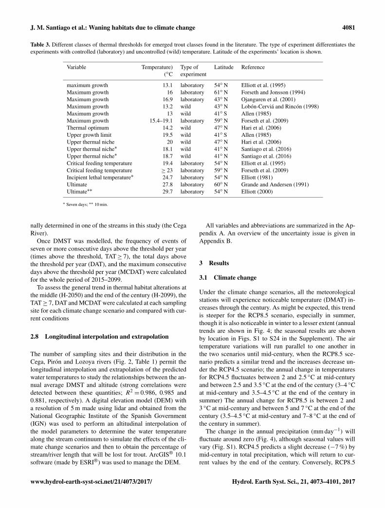
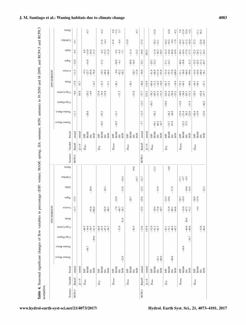
Statistically significant (p < 0.05) shifts in the flow regimewill be rare in H-2050 (Table 4, Fig. 5). In H-2099, thesechanges will be less pronounced, but significant changes be-
come more frequent (Table 4, Fig. 5). Only two gauging sta-tions (Lozoya and Tagus) exhibit significant reductions inannual discharge. By the end of the century (H-2099), an-nual discharge is expected to be significantly lower at sevengauging stations. The Tagus Basin will experience the great-est changes in annual discharge. Maximum, mean and mini-mum daily discharges (Qmean andQmin), as well as the Q10,will become much lower in Tagus River basin. Only Cega-Lastras and Pirón (Duero River basin) will suffer a significantincrease in the number of zero-flow days.
3.2.2 RCP8.5 scenario
According to the predictions, the most significant changesin flow regimes will occur at the gauging stations of Cega-Lastras and Lozoya in H-2050 (Table 4, Fig. 5). In H-2099, most sites will experience strong flow reductions, evenin seasons where seasonal increases in flow are predicted(e.g. Ebrón and both stations in the Tormes River) (Table 4,Fig. 5). Significant annual runoff reductions in H-2050 willoccur at five of the stations, increasing the occurrence of sig-nificant losses at 9 out of the 10 sites in H-2099 (i.e. all sta-tions except Ebrón). The most important decreases in everyvariable and throughout the century were predicted for thestations in the middle Cega Basin and the Tagus Basin. Asignificant increase in the number of days with no flow waspredicted for Cega-Lastras, Pirón and Gallo.
3.2.3 Geographical pattern
The cluster analysis of gauging stations based on seasonalvariations in the flow regime revealed the importance ofcareful examinations at the local level, since hydrologi-cal behaviour is a consequence of both macroclimatic andmesoclimatic conditions. A geographical pattern is recog-nizable when the actual flow regime (2006–2015) is season-ally clustered (Fig. 6). Analysing the deviations in this ge-ographical pattern by scenarios and horizons, the differentgauging stations can grouped according to the seasonal be-haviour of the flow changes (Fig. 7a). For the RCP4.5 sce-nario in H-2050 (agglomerative coefficients, a.c.= 0.73), thestations that differed most strongly from the remainder interms of their deviations in the flow regime are those locatedat Cega-Lastras (winter), Pirón (autumn) and Ebrón (sum-mer). For RCP4.5 in H-2099 (a.c.= 0.56), they are Cega-Pajares (spring), Tormes-Hoyos (summer) and Ebrón (au-tumn). For RCP8.5 in H-2050 (a.c.= 0.61), they are Pirón(spring, summer and autumn), Lozoya and Ebrón (both inwinter). For RCP8.5 in H-2099 (a.c.= 0.72), they are Cega-Pajares (spring) and Ebrón (summer, autumn and winter).
Hydrol. Earth Syst. Sci., 21, 4073–4101, 2017 www.hydrol-earth-syst-sci.net/21/4073/2017/
J. M. Santiago et al.: Waning habitats due to climate change 4083
Tabl
e4.
Seas
onal
sign
ifica
ntch
ange
sof
flow
vari
able
sin
perc
enta
ge(D
JF:
win
ter;
MA
M:
spri
ng;
JJA
:su
mm
er;
SON
:au
tum
n)in
H-2
050
and
H-2
099,
and
RC
P4.5
and
RC
P8.5
scen
ario
s.
2050
HO
RIZ
ON
2099
HO
RIZ
ON
Scen
ario
Var
iabl
ePe
riod
Tormes-Hoyos
Tormes-Barco
Cega-Pajares
Cega-Lastras
Pirón
Lozoya
Tagus
Gallo
Cabrillas
Ebrón
Scen
ario
Var
iabl
ePe
riod
Tormes-Hoyos
Tormes-Barco
Cega-Pajares
Cega-Lastras
Pirón
Lozoya
Tagus
Gallo
Cabrillas
Ebrón
RC
P4.5
Run
off
annu
al−
11.7−
13.5
RC
P4.5
Run
off
annu
al−
11.3
−8.
6−
17.0
−11
.5−
12.9
−6.
5−
9.1
Q=
0an
nual
Q=
0an
nual
85.8
42.7
Qm
inD
JF−
49.5
Qm
inD
JF−
9.3
8.9
MA
M−
56.7
−34
.6M
AM
−28
.8−
29.2
−22
.7−
14.8−
13.0
−8.
7JJ
A−
39.7
−93
.8−
28.0
JJA
−9.
9−
85.0
−18
.0SO
N−
50.6−
41.4
−10
6.0
SON
−14
.7−
76.8
−11
.5
Q10
DJF
−44
.8Q
10D
JF−
27.8
MA
M−
25.4
MA
M−
10.5−
25.2
−19
.4−
23.3
−19
.2−
17.2
−8.
2−
11.6
−6.
2JJ
A−
43.3
−92
.9−
18.3
JJA
−23
.8−
48.6
−15
.2−
6.3
SON
−36
.7−
98.1
SON
−17
.1−
86.9
−11
.0
Qm
ean
DJF
Qm
ean
DJF
−11
.66.
8M
AM
−7.
9−
22.0
MA
M−
10.5−
15.1
−28
.1−
9.0−
20.9
−9.
2−
5.3
JJA
−33
.9−
48.7
JJA
−37
.3−
42.2
−6.
1−
6.5
−8.
45.
7SO
N−
32.9
51.6
−26
.1−
13.0−
16.4
SON
−26
.2−
7.1
Qm
axD
JFQ
max
DJF
−15
.9M
AM
−28
.7M
AM
−30
.1−
20.9−
11.4
JJA
−30
.319
.6JJ
A−
27.8
−20
.7−
18.5
SON
−34
.7SO
N−
17.0
−13
.2−
8.7
RC
P8.5
Run
off
annu
al−
13.6
−15
.5−
25.8−
12.2−
12.7
RC
P8.5
Run
off
annu
al−
7.7−
12.5−
12.5−
37.7−
48.6
−39
.0−
32.1−
19.0−
17.5
Q=
0an
nual
147.
6Q=
0an
nual
332.
211
6.9
203.
5
Qm
inD
JF−
32.9
Qm
inD
JF−
30.7−
58.3−
69.4
−41
.8−
29.3
MA
M−
41.3
−39
.4−
12.1
MA
M−
38.1−
38.2
−69
.5−
31.2
−68
.9−
32.2−
11.6−
18.3−
12.0
JJA
−43
.1−
42.7
−73
.8−
33.9
JJA
66.2
−53
.3−
14.2−
111.
8−
36.2−
13.1
SON
−88
.0−
49.7
SON
24.7
−51
.4−
16.0
−93
.8−
30.5
Q10
DJF
−43
.1−
23.5
Q10
DJF
−24
.0−
62.9−
62.7
−37
.0−
37.1−
12.4−
16.2
MA
M−
33.1
−31
.9−
19.6
−8.
8M
AM
−33
.7−
36.2
−61
.4−
33.3
−55
.3−
34.7−
14.6−
19.2
14.8
JJA
−40
.6−
48.4
−89
.1−
17.9
JJA
67.9
46.8
−50
.4−
72.0
−28
.0−
9.4
SON
−45
.2−
94.6
SON
−53
.2−
18.9−
108.
0−
19.9
−7.
9−
6.2
Qm
ean
DJF
−30
.3−
17.1
Qm
ean
DJF
−23
.4−
12.9−
40.0−
55.3
−21
.1−
40.4−
20.3−
19.2
5.8
MA
M−
16.6
−15
.0−
35.4
−9.
7M
AM
−22
.5−
21.4
−28
.9−
49.3
−38
.0−
38.8−
19.4−
16.7−
12.9
JJA
−44
.028
.6−
47.2
−10
.0−
8.5
JJA
27.5
28.5
−65
.7−
80.2
−17
.0−
11.2
12.6
SON
−34
.7−
40.6
−31
.1−
14.5
SON
−22
.0−
37.4−
51.5−
50.6
−59
.6−
21.5−
17.5−
18.0
−4.
4
Qm
axD
JF−
30.9
Qm
axD
JF−
26.4
−20
.5−
44.3
−14
.4−
32.5−
32.5−
27.2
MA
M−
9.4−
33.9
MA
M−
12.9
−50
.1−
24.6−
24.5−
26.2
−11
.1JJ
A−
33.6
JJA
−62
.8−
66.9−
21.2−
11.7−
22.8
26.2
SON
−40
.4−
22.3
SON
−23
.0−
40.2−
47.7−
47.7
−38
.1−
45.7−
24.3−
24.6
www.hydrol-earth-syst-sci.net/21/4073/2017/ Hydrol. Earth Syst. Sci., 21, 4073–4101, 2017

4084 J. M. Santiago et al.: Waning habitats due to climate change
Figure 5. Predicted monthly mean specific flow in H-2050 and H-2099 for the RCP4.5 and RCP8.5 scenarios. Shaded areas indicate decadalfluctuations. Triangles show significant negative or positive trends (Sen’s slope p≤ 0.05); the sign of each trend is indicated by the directionsin which the triangles point.
3.3 Stream temperature
3.3.1 Model parameter behaviour and general trends
The inclusion of the streamflow component improves modelperformance at 12 out of the 28 study sites (Table 5). In theremaining 16 cases, either no convergence of values was ob-
served in the regression process or the obtained values did notimprove the results, as the streamflow component (Term 2of the equation) is virtually zero at the other sites. The five-parameter model was used in these remaining 16 cases. Thecalculated parameters and the performance indicators (RSEand NSE) of the models are shown in Table 6, and daily meanstream temperatures estimated by the climate change models
Hydrol. Earth Syst. Sci., 21, 4073–4101, 2017 www.hydrol-earth-syst-sci.net/21/4073/2017/
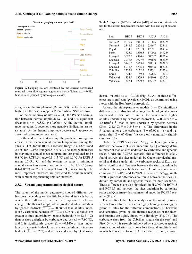
J. M. Santiago et al.: Waning habitats due to climate change 4085
0.8 0.6 0.4 0.2 0.0
Clustered gauging stations: year 2015
Tormes−Barco
Cabrillas
Gallo
Ebrón
Cega−Lastras
Pirón
Tagus
Lozoya
Tormes−Hoyos
Cega−PajaresStation
Station
Station
detrital
carbonate
igneousLithological classes
Figure 6. Gauging stations clustered by the current normalizedseasonal streamflow regime (agglomerative coefficient, a.c.= 0.81).Stations are grouped by lithological classes.
are given in the Supplement (Dataset S3). Performance washigh in all the cases except in Pirón 5 where NSE was low.
For the entire array of sites (n= 31), the Pearson correla-tion between thermal amplitude (α−µ) and λ is significant(Pearson’s r =−0.832; p < 0.0001). As the thermal ampli-tude increases, λ becomes more negative (indicating less re-sistance). As the thermal amplitude decreases, λ approacheszero (indicating more resistance).
By the end of the 21st century, the predicted average in-crease in the mean annual stream temperature among thesites is 1.1 ◦C for the RCP4.5 scenario (range 0.3–1.6 ◦C) and2.7 ◦C for RCP8.5 (range 0.8–4.0 ◦C). The average increasesin maximum annual mean temperature are predicted to be0.8 ◦C for RCP4.5 (range 0.1–1.5 ◦C) and 1.6 ◦C for RCP8.5(range 0.2–3.0 ◦C), and the average increases in minimumannual mean temperature are predicted to be 1.0 ◦C (range0.4–1.8 ◦C) and 2.7 ◦C (range 1.1–4.5 ◦C), respectively. Themost important increases are predicted to occur in winter,with summer experiencing smaller increases.
3.3.2 Stream temperature and geological nature
The values of the model parameters showed different be-haviours depending on the lithology found in each basin,which thus influences the thermal response to climatechange. The thermal amplitude is greater at sites underlainby igneous bedrock (α−µ= 20.38 ◦C) than at sites under-lain by carbonate bedrock (α−µ= 13.07 ◦C). β values aregreater at sites underlain by igneous bedrock (β = 12.71 ◦C)than at sites underlain by carbonate bedrock (β = 7.80 ◦C),and λ is significantly greater (λ=−0.140) at sites under-lain by carbonate bedrock than at sites underlain by igneousbedrock (λ=−0.292) and at sites underlain by Quaternary
Table 5. Bayesian (BIC) and Akaike (AIC) information criteria val-ues for the stream-temperature models with five and eight parame-ters.
Site BIC 5 BIC 8 AIC 5 AIC 8
Tormes2 2075.7 1911.8 2108.5 1837.9Tormes3 2346.7 2274.2 2346.7 2234.8Cega1 1814.8 1731.9 1789.1 1693.4Pirón1 1725.9 1530.5 1700.2 1492.0Lozoya1 5097.3 4924.6 5065.2 4876.4Lozoya2 3979.3 3927.9 3948.6 3881.9Lozoya3 3841.6 3673.6 3811.5 3628.5Lozoya4 5076.6 4735.3 5044.8 4687.5Cabrillas 2552.9 2172.2 2523.1 2127.4Ebrón 624.8 169.8 598.5 130.3Vallanca1 1438.9 1359.9 1410.6 1317.3Vallanca2 1322.1 1279.7 1293.7 1237.1
detrital material (λ=−0.305) (Fig. 8). All of these differ-ences are significant (p-values < 0.001, as determined usingt tests with the Bonferroni correction).
Among the eight-parameter models (n= 12), significantdifferences are also found among the lithological classesfor ω and τ . For both ω and τ , the values were higherat sites underlain by carbonate bedrock (ω = 0.96 ◦C; τ =3.640 m3 s−1) than at sites underlain by igneous bedrock(ω =−2.12 ◦C; τ = 0.345 m3 s−1). The differences in theδ values among the carbonate (δ = 67.06 m−3 s) and ig-neous sites (δ = 67.06 m−3 s) were only marginally signifi-cant (p < 0.1).
Under the RCP4.5 scenario, 1Tmin displays significantlydifferent behaviour at sites underlain by Quaternary detri-tal material than at sites underlain by carbonate and igneousrocks. Under the RCP8.5 scenario, this difference is solelyfound between the sites underlain by Quaternary detrital ma-terial and those underlain by carbonate rocks. 1Tmean ex-hibits significant differences between the sites underlain byall three lithologies in both scenarios. All of these results arecommon to H-2050 and H-2099. In terms of 1Tmax, in H-2050, significant differences are found between the sites un-derlain by carbonate and igneous rocks for both scenarios.These differences are also significant in H-2099 for RCP4.5and RCP8.5 and between the sites underlain by carbonaterocks and Quaternary detrital material under the RCP8.5 sce-nario (Fig. 9).
The results of the cluster analysis of the monthly meanstream temperatures revealed a highly homogeneous aggre-gation of sites for the different combinations of horizonsand scenarios, given that the thermal responses of the riversand streams are tightly linked with lithology (Fig. 7b). Thecarbonate sites from the Cabrillas stream (in the east) andPirón 3 (which is strongly influenced by a calcareous spring)form a group of sites that shows low thermal amplitude andin which λ is close to zero. At the other extreme, a group
www.hydrol-earth-syst-sci.net/21/4073/2017/ Hydrol. Earth Syst. Sci., 21, 4073–4101, 2017

4086 J. M. Santiago et al.: Waning habitats due to climate change
Figure 7. Study sites clustered by the predicted change ratios of the seasonal mean streamflow (gauging stations) and by the predictedincrease in the monthly mean stream temperature (◦C) at the water temperature recording sites in H-2050 and H-2099 for the RCP4.5 andRCP8.5 scenarios. Axes indicate geographic positions (UTM coordinates). The colours and numbers indicate the clusters.
that is made up mainly of sites underlain by igneous material(in the Lozoya and Tormes basins, in addition to several sitesfound in the detrital basin of Cega-Pirón) shows higher ther-mal amplitude and lower values of λ than the former group.
The remaining sites have intermediate values of thermal am-plitude and resistance.
Hydrol. Earth Syst. Sci., 21, 4073–4101, 2017 www.hydrol-earth-syst-sci.net/21/4073/2017/

J. M. Santiago et al.: Waning habitats due to climate change 4087
Table 6. Parameter values of the stream temperature models for every thermograph site (λ is a dimensionless parameter) and values of theperformance indicators residual standard error (RSE) and Nash–Sutcliffe efficiency index (NSE).
Site µ α α−µ γ β λ ω δ τ RSE NSE(◦C) (◦C) (◦C) (◦C−1) (◦C) (◦C) (m−3 s) (m3 s−1) (◦C)
Aravalle 0.1 23.3 23.2 0.14 10.79 −0.31 2.31 0.70Barbellido 1.1 19.2 18.1 0.23 12.19 −0.30 3.29 0.81Gredos Gorge 2.4 19.0 16.6 0.18 14.06 −0.29 3.68 0.71Tormes1 −1.1 20.8 21.9 0.16 11.00 −0.35 1.97 0.83Tormes2 3.4 24.6 21.3 0.14 11.82 −0.31 −3.98 61.43 0.37 1.56 0.78Tormes3 −0.1 30.5 30.6 0.12 12.61 −0.39 −2.85 223.69 0.22 1.62 0.79Pirón1 −1.4 19.1 20.5 0.09 14.33 −0.18 −2.08 72.82 0.15 0.97 0.91Pirón2 0.6 15.5 14.9 0.22 12.11 −0.23 3.69 0.82Pirón3 7.2 14.0 6.8 0.29 10.17 −0.10 1.16 0.77Pirón4 −0.6 18.3 18.9 0.15 8.20 −0.29 1.26 0.85Pirón5 −4.6 21.7 26.3 0.13 8.92 −0.40 1.57 0.39Cega1 1.4 15.6 14.2 0.19 15.92 −0.22 −1.53 112.98 0.27 1.17 0.88Cega2 −0.6 18.0 18.6 0.17 16.03 −0.31 1.81 0.85Cega3 −2.0 24.7 26.6 0.14 15.35 −0.41 2.83 0.85Cega4 −0.3 19.9 20.2 0.16 12.21 −0.35 1.65 0.87Cega5 −2.4 18.1 20.5 0.13 7.85 −0.31 0.87 0.84Cega6 0.7 22.4 21.7 0.13 13.84 −0.38 2.34 0.79Lozoya1 0.4 19.5 19.1 0.18 11.90 −0.24 −1.33 11.93 0.41 1.13 0.90Lozoya2 0.3 20.2 20.0 0.19 11.63 −0.28 −1.27 13.16 0.38 1.17 0.90Lozoya3 1.1 21.0 19.9 0.19 10.62 −0.29 −1.74 23.44 0.49 1.23 0.89Lozoya4 1.7 22.0 20.2 0.17 10.29 −0.27 −2.19 17.04 0.48 1.17 0.90Tagus-Peralejos 1.1 21.0 19.9 0.11 11.01 −0.17 1.00 0.89Tagus-Poveda 1.3 20.4 19.2 0.15 9.95 −0.38 1.26 0.83Gallo 0.4 20.2 19.8 0.13 7.76 −0.18 0.90 0.92Cabrillas 8.3 15.3 7.0 0.21 9.23 −0.04 −1.38 13.56 1.25 1.65 0.90Ebrón 5.5 17.0 11.4 0.07 6.58 −0.06 1.73 −1.78 3.16 0.27 0.86Vallanca1 −0.5 16.9 17.4 0.09 4.70 −0.12 1.95 −5.21 4.85 0.53 0.88Vallanca2 1.4 16.8 15.4 0.10 5.36 −0.11 1.54 −11.29 5.29 0.50 0.89Palancia1 11.7 15.3 3.6 0.19 13.92 −0.03 0.23 0.93Palancia2 9.3 16.1 6.8 0.27 12.73 −0.11 0.59 0.88Villahermosa 7.8 18.0 10.2 0.27 16.46 −0.20 1.02 0.85
3.3.3 Effect of streamflow reductions on streamtemperature
The predicted flow reductions lead to notable increasesin water temperature. The effect of streamflow variationon stream temperature is analysed at the following sites:Tormes 2, Tormes 3, Pirón 1, Cega 1, Lozoya 1 to 4, Cabril-las, Ebrón 1 and Vallanca 1 and 2. These are the sites at whichthe eight-parameter model improves upon the five-parametermodel. In all cases, differences in stream temperature be-tween the five- and eight-parameter models are found, andsummer flow reductions lead to increases in stream temper-ature, increasing DAT, TAT≥ 7 and MCDAT. Among thesesites, the threshold is only surpassed at Lozoya and Tormes,increasing the thermal habitat loss. At Cega 1, Cabrillas andEbrón, α is below the thermal threshold, and at Pirón 1, thestream temperature increase is not sufficient to exceed thethreshold.
For all of the sites at which the influence of streamflow onstream temperature was revealed, the eight-parameter modelestimates higher values of maximum annual DMST than thefive-parameter model. The maximum annual DMST calcu-lated by the eight-parameter model is 3.6 ◦C higher than thatcalculated by the five-parameter model at the Tormes 2 site.This difference is not so large at the other sites, and the mini-mum disagreement between the models (0.01 ◦C) is noted atthe Ebrón and Cabrillas sites. In general, the maximum dif-ferences between the two models are noted in igneous catch-ments, whereas carbonate sites yield the lowest differences.
3.3.4 Effect of climate change on the thermal habitat ofbrown trout
The length of the thermal habitat of trout will undergo impor-tant reductions due to the rises in water temperatures and theincrease in the extent of the warm period. In the predictionsfor H-2050, the 18.7 ◦C threshold (TAT≥ 7) will be violated
www.hydrol-earth-syst-sci.net/21/4073/2017/ Hydrol. Earth Syst. Sci., 21, 4073–4101, 2017
4088 J. M. Santiago et al.: Waning habitats due to climate change
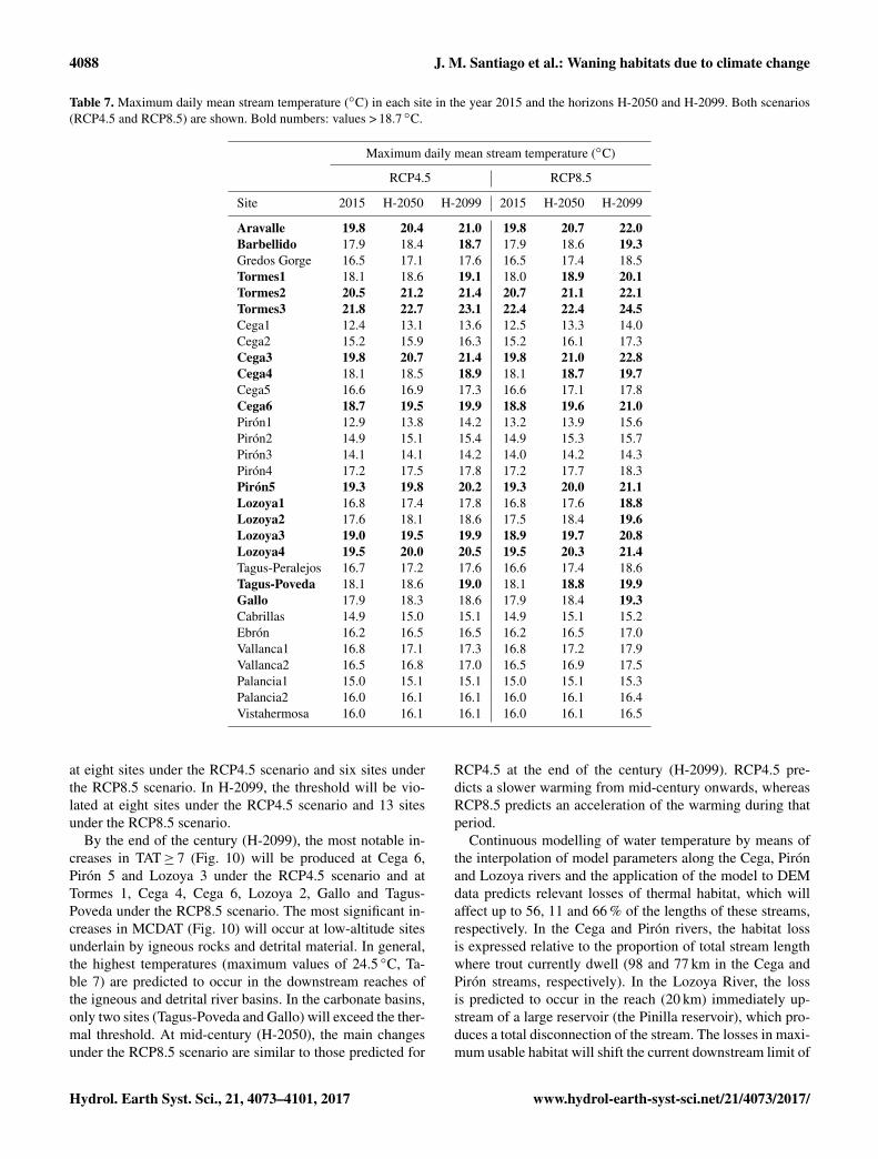
Table 7. Maximum daily mean stream temperature (◦C) in each site in the year 2015 and the horizons H-2050 and H-2099. Both scenarios(RCP4.5 and RCP8.5) are shown. Bold numbers: values > 18.7 ◦C.
Maximum daily mean stream temperature (◦C)
RCP4.5 RCP8.5
Site 2015 H-2050 H-2099 2015 H-2050 H-2099
Aravalle 19.8 20.4 21.0 19.8 20.7 22.0Barbellido 17.9 18.4 18.7 17.9 18.6 19.3Gredos Gorge 16.5 17.1 17.6 16.5 17.4 18.5Tormes1 18.1 18.6 19.1 18.0 18.9 20.1Tormes2 20.5 21.2 21.4 20.7 21.1 22.1Tormes3 21.8 22.7 23.1 22.4 22.4 24.5Cega1 12.4 13.1 13.6 12.5 13.3 14.0Cega2 15.2 15.9 16.3 15.2 16.1 17.3Cega3 19.8 20.7 21.4 19.8 21.0 22.8Cega4 18.1 18.5 18.9 18.1 18.7 19.7Cega5 16.6 16.9 17.3 16.6 17.1 17.8Cega6 18.7 19.5 19.9 18.8 19.6 21.0Pirón1 12.9 13.8 14.2 13.2 13.9 15.6Pirón2 14.9 15.1 15.4 14.9 15.3 15.7Pirón3 14.1 14.1 14.2 14.0 14.2 14.3Pirón4 17.2 17.5 17.8 17.2 17.7 18.3Pirón5 19.3 19.8 20.2 19.3 20.0 21.1Lozoya1 16.8 17.4 17.8 16.8 17.6 18.8Lozoya2 17.6 18.1 18.6 17.5 18.4 19.6Lozoya3 19.0 19.5 19.9 18.9 19.7 20.8Lozoya4 19.5 20.0 20.5 19.5 20.3 21.4Tagus-Peralejos 16.7 17.2 17.6 16.6 17.4 18.6Tagus-Poveda 18.1 18.6 19.0 18.1 18.8 19.9Gallo 17.9 18.3 18.6 17.9 18.4 19.3Cabrillas 14.9 15.0 15.1 14.9 15.1 15.2Ebrón 16.2 16.5 16.5 16.2 16.5 17.0Vallanca1 16.8 17.1 17.3 16.8 17.2 17.9Vallanca2 16.5 16.8 17.0 16.5 16.9 17.5Palancia1 15.0 15.1 15.1 15.0 15.1 15.3Palancia2 16.0 16.1 16.1 16.0 16.1 16.4Vistahermosa 16.0 16.1 16.1 16.0 16.1 16.5
at eight sites under the RCP4.5 scenario and six sites underthe RCP8.5 scenario. In H-2099, the threshold will be vio-lated at eight sites under the RCP4.5 scenario and 13 sitesunder the RCP8.5 scenario.
By the end of the century (H-2099), the most notable in-creases in TAT≥ 7 (Fig. 10) will be produced at Cega 6,Pirón 5 and Lozoya 3 under the RCP4.5 scenario and atTormes 1, Cega 4, Cega 6, Lozoya 2, Gallo and Tagus-Poveda under the RCP8.5 scenario. The most significant in-creases in MCDAT (Fig. 10) will occur at low-altitude sitesunderlain by igneous rocks and detrital material. In general,the highest temperatures (maximum values of 24.5 ◦C, Ta-ble 7) are predicted to occur in the downstream reaches ofthe igneous and detrital river basins. In the carbonate basins,only two sites (Tagus-Poveda and Gallo) will exceed the ther-mal threshold. At mid-century (H-2050), the main changesunder the RCP8.5 scenario are similar to those predicted for
RCP4.5 at the end of the century (H-2099). RCP4.5 pre-dicts a slower warming from mid-century onwards, whereasRCP8.5 predicts an acceleration of the warming during thatperiod.
Continuous modelling of water temperature by means ofthe interpolation of model parameters along the Cega, Pirónand Lozoya rivers and the application of the model to DEMdata predicts relevant losses of thermal habitat, which willaffect up to 56, 11 and 66 % of the lengths of these streams,respectively. In the Cega and Pirón rivers, the habitat lossis expressed relative to the proportion of total stream lengthwhere trout currently dwell (98 and 77 km in the Cega andPirón streams, respectively). In the Lozoya River, the lossis predicted to occur in the reach (20 km) immediately up-stream of a large reservoir (the Pinilla reservoir), which pro-duces a total disconnection of the stream. The losses in maxi-mum usable habitat will shift the current downstream limit of
Hydrol. Earth Syst. Sci., 21, 4073–4101, 2017 www.hydrol-earth-syst-sci.net/21/4073/2017/

J. M. Santiago et al.: Waning habitats due to climate change 4089
Figure 8. Distributions of the stream temperature model parame-ter values (α−µ, β, γ and λ) in relation to lithology. Differenceswere assessed using Student’s t test with the Bonferroni correction(p < 0.05).
the trout distribution from 820 up to 831 m a.s.l in the PirónRiver, from 730 up to 830 m a.s.l. in the Cega River, and from1090 up to 1276 m a.s.l. in the Lozoya River. In the particularcase of the Cega River, a window of usable thermal habitat isalso predicted to occur upstream from this altitudinal range(from 913 up to 1050 m a.s.l.).
4 Discussion
4.1 Climate change
Our downscaled results predict greater air temperature incre-ments than the original IPCC (2013) results. These highertemperatures may lead to increased ecological impacts (Mag-nuson and Destasio, 1997; Angilletta, 2009) caused by thecombination of rising water temperatures and decreasingstream flows. The results from the AR5 of the IPCC and itsannex, the Atlas of Global and Regional Climate Projections(IPCC, 2013), suggest that droughts are unlikely to increasein the near future for the Mediterranean area. However, airtemperatures are expected to rise, subsequently increasingevapotranspiration. As a consequence, the available water inrivers and streams will be reduced. Regional studies haveused coarser resolutions than ours, which may be appropriatefor their goals (e.g. Thuiller et al., 2006). However, they maybe insufficient when more local predictions are needed, asdoes our study, which treats geographically confined, stream-dwelling trout populations. Therefore, fine downscaling tech-niques like those applied in this study must be used whenhigh-resolution, detailed predictions are needed.
4.2 Streamflow
This study predicts significant but diverse streamflow reduc-tions during the present century. At the regional level, a re-duction in water resources is expected in the Mediterraneanarea (IPCC, 2013). Milly et al. (2005) predicted a 10–30 %decrease in runoff in southern Europe in 2050. In anotherglobal-scale study, van Vliet et al. (2013) predicted a de-crease in the mean flows of greater than 25 % in the IberianPeninsula area by the end of the century (2071–2100), us-ing averages for both the SRES A2 and B1 scenarios (Na-kicenovic et al., 2000). Our results predict mean flows thatare similar to that value (−23 %; range: 0–49 %), althoughthe emissions scenarios in this study are more severe (thatis, they involve greater increases in atmospheric CO2) thanthose used in the aforementioned studies.
More specifically, the predictions for the RCP4.5 scenarioshow flow reductions that range from negligibly small to sig-nificant (up to 17 %). Under the RCP8.5 scenario, significantreductions become more widespread, ranging up to 49 % ofthe annual streamflow losses. Our results also predict a rele-vant increase in the number of days with zero flow for somestations in the detrital area under this scenario (RCP8.5). Thepredicted streamflow changes are compatible with those ob-tained in previous studies, although these studies were per-formed at larger scales (Milly et al., 2005; van Vliet et al.,2013). The apparent differences between the streamflow re-ductions estimated in this study and those obtained by Millyet al. (2005) and van Vliet et al. (2013) (who report lowerflow reductions than those given in the present study) mightbe caused by the regional focus of their predictions (the en-tire Iberian Peninsula), whereas ours are focused on moun-tain reaches.
In terms of methods, process-based hydrological modelsare often preferred for climate change studies (Van Vliet etal., 2012). However, they can be overly complicated and re-quire excessive data inputs, which may also lead to over-fitting of the data (Zhuo et al., 2015). Constraining furtherpredictions to within the training domain is a rule of thumbfor machine learning studies (Fielding, 1999), although ex-trapolation is rather common (Elith and Leathwick, 2009).Therefore, taking into account the extrapolation that occurstowards lower flows, which are over-represented in the train-ing dataset, we consider the magnitude of the extrapolationacceptable, and we consider the values, although they are notexempt from uncertainty, to be reliable.
4.3 Stream temperature
The model we present in this study showed good perfor-mance. Bustillo et al. (2013) recommended the assessmentof the impacts of climate change on river temperatures us-ing regression-based methods like ours that rely on logisticapproximations of equilibrium temperatures (Edinger et al.,
www.hydrol-earth-syst-sci.net/21/4073/2017/ Hydrol. Earth Syst. Sci., 21, 4073–4101, 2017

4090 J. M. Santiago et al.: Waning habitats due to climate change
Figure 9. Distributions of 1Tmin, 1Tmean and 1Tmax in relation to lithology for the climate change scenarios RCP4.5 and RCP8.5 inH-2050 and H-2050. The reference period corresponds to the simulated period 2010–2019.
1968), which are at least as robust as the most refined classi-cal heat balance models.
However, we also sought to identify relationships betweenthermal regime and other environmental variables besidesair temperature and streamflow, such as geology. Bogan etal. (2003) showed that water temperatures were uniquelycontrolled by climate in only 26 % of 596 studied streamreaches. Groundwater, wastewater and reservoir releases in-fluenced water temperatures in the remaining 74 % of thecases. Loinaz et al. (2013) quantified the influence of ground-water discharge on temperature variations in the Silver CreekBasin (Idaho, USA), and they concluded that a 10 % reduc-tion in groundwater flow can cause increases of over 0.3and 1.5 ◦C in the average and maximum stream tempera-tures, respectively. Our studied reaches were not influencedby wastewater or reservoir releases (with the exception ofreleases from the Torrecaballeros Dam on the Pirón River).Kurylyk et al. (2015) showed that the temperature of shallowgroundwater influences the thermal regimes of groundwater-dominated streams and rivers. Since groundwater is stronglyinfluenced by geology, we can expect it to be a good indi-cator of the thermal response, as shown here. The modelsused accurately described the thermal performance of thestudy sites, and we found significant relationships among themodel parameters, the underlying lithologies and the hydro-logic responses. Thermal amplitude (α−µ) and temperatureat the maximum change rate (β) were lower, and the resis-tance parameter (λ) was closer to zero, in river basins thatwere highly influenced by aquifers (mainly carbonate) com-pared to the others, particularly compared with river basinsunderlain by carbonate rocks. Since DMST is a variable thatis relevant for detecting departures from thermal niche, wecan conclude that it is worthwhile to use the more complex
eight-parameter model to predict the effects of global warm-ing, especially in igneous catchments.
A wide range of models is described in the literature, andeach such model has its strengths and weaknesses. Arismendiet al. (2014) hold that regression models based on air temper-ature can be inadequate for projecting future stream temper-atures because they are only surrogates for air temperature,whereas Piccolroaz et al. (2016) argued that the adequacydepends on the hydrological regime, type of model and thetimescale analysis. Their main objections to regressive meth-ods arose when modelling reaches of regulated rivers, but thisis not our case. In addition, our model improves the mod-els that were tested in both studies (Arismendi et al., 2014;Piccolroaz et al., 2016). Performance indicators of our mod-els produce good results, showing that the models are suffi-ciently competent. We show that our model implicitly inte-grates the effect of other factors, such as geology and flowregime by means of its parameters. A fine mechanistic solu-tion to the modelling issue could need prohibitive methods(Kurylyk et al., 2015), losing the advantages that make at-tractive the model (input data easy to get). Therefore a com-promise between improved precision and increased cost mustbe met.
The behaviour and dynamics of the parameters offer apromising research field. Their analysis may help to intro-duce new parametrization criteria to avoid the risk of ignor-ing the effect of climate warming on groundwater (subsur-face water and deep water), for instance. The thermal sen-sitivity of shallow groundwater differs between short-term(e.g. seasonal) and long-term (e.g. multi-decadal) time hori-zons, and the relationship between air and water tempera-tures does not necessarily reflect this difference. This vari-ability should be taken into account in order to avoid un-
Hydrol. Earth Syst. Sci., 21, 4073–4101, 2017 www.hydrol-earth-syst-sci.net/21/4073/2017/
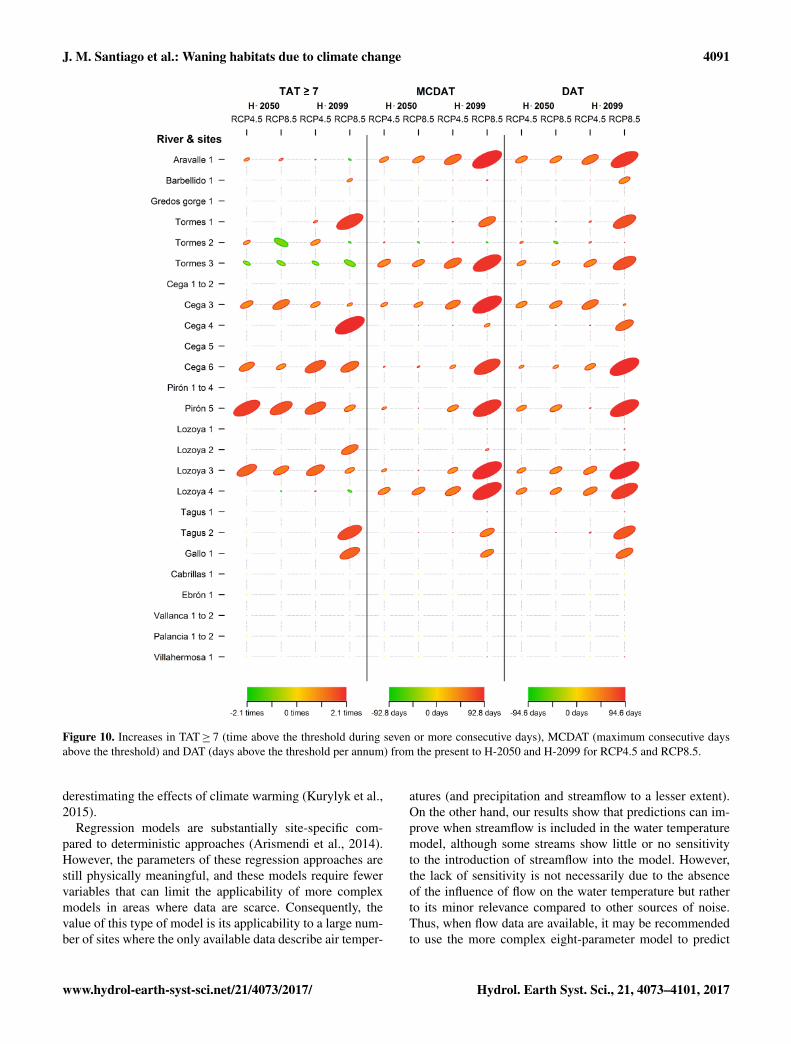
J. M. Santiago et al.: Waning habitats due to climate change 4091
Figure 10. Increases in TAT≥ 7 (time above the threshold during seven or more consecutive days), MCDAT (maximum consecutive daysabove the threshold) and DAT (days above the threshold per annum) from the present to H-2050 and H-2099 for RCP4.5 and RCP8.5.
derestimating the effects of climate warming (Kurylyk et al.,2015).
Regression models are substantially site-specific com-pared to deterministic approaches (Arismendi et al., 2014).However, the parameters of these regression approaches arestill physically meaningful, and these models require fewervariables that can limit the applicability of more complexmodels in areas where data are scarce. Consequently, thevalue of this type of model is its applicability to a large num-ber of sites where the only available data describe air temper-
atures (and precipitation and streamflow to a lesser extent).On the other hand, our results show that predictions can im-prove when streamflow is included in the water temperaturemodel, although some streams show little or no sensitivityto the introduction of streamflow into the model. However,the lack of sensitivity is not necessarily due to the absenceof the influence of flow on the water temperature but ratherto its minor relevance compared to other sources of noise.Thus, when flow data are available, it may be recommendedto use the more complex eight-parameter model to predict
www.hydrol-earth-syst-sci.net/21/4073/2017/ Hydrol. Earth Syst. Sci., 21, 4073–4101, 2017

4092 J. M. Santiago et al.: Waning habitats due to climate change
the effects of climate warming. This conclusion is especiallyapplicable to lithologically sensitive basins, such as those un-derlain by igneous rocks.
The predicted increase in water temperature will be sub-stantial at most of the study sites. The annual mean rates ofchange will increase with time. Stewart et al. (2015) predictan increase of 1–2 ◦C by mid-century in 80 % of the streamlengths in Wisconsin and by 1–3 ◦C by the latter part of thecentury in 99 % of the stream lengths, which corresponds toa significant loss in suitable areas for cold-water fish. The re-sults of Stewart et al. (2015) do not differ from ours, exceptthat we expect greater increases by the end of the studied pe-riod (up to 4 ◦C). Our results are also compatible with thoseof van Vliet et al. (2013), who predicted a water temperatureincrease > 2 ◦C in the Iberian Peninsula area by the end of thecentury; however, our results are more specific and precise.In this sense, Muñoz-Mas et al. (2016) also obtained similarresults for H-2050 in a river reach in central Spain by mid-century (i.e. daily mean flow reductions between 20 and 29 %and daily mean stream temperature increases up to 0.8 ◦C).However, we predict that the minima are more sensitive toclimate warming than the maxima.
4.4 Effects of climate change on brown troutpopulations
Brown trout are sensitive to changes in discharge patterns be-cause high-intensity floods during the incubation and emer-gence periods may limit recruitment (Lobón-Cerviá andRincón, 2004; Junker et al., 2015). In the Iberian Penin-sula, the trout distribution is mainly concentrated in moun-tain streams, where extreme discharges during winter are ex-pected to increase (Rojas et al., 2012). These extreme dis-charges will likely affect trout recruitment negatively. Thus,the predicted changes in the hydrological regime can subjectbrown trout populations to more variable conditions, whichmay occasionally present some populations with insupera-ble bottlenecks. Trout are polytypic and display an adapt-able phenology and rather high intra-population variabilityin their life history traits that might allow them to show re-silience to variations in habitat features (Gortázar et al., 2007;Larios-López et al., 2015), especially in the marginal ranges(Ayllón et al., 2016). However, despite these strong evolu-tionary responses, the current combination of warming andstreamflow reduction scenarios is likely to exceed the capac-ity of many populations to adapt to new conditions (Ayllón etal., 2016). Consistent with regional predictions (Rojas et al.,2012; Garner et al., 2015), significant flow reductions are ex-pected during summertime in most of the studied rivers andstreams at the end of the century, and this may mean, in turn,the reduction in the suitable habitat (i.e. the available watervolume) (Muñoz-Mas et al., 2016). Finally, the increase inextreme droughts, which involve absolute water depletion, incertain reaches of the streams may be critical for some troutpopulations.
The predicted increase in winter stream temperatures canaffect the sessile phases (i.e. eggs and larvae) of trout de-velopment. These phases are very sensitive to temperaturechanges because it affects their physiology, and because theirdevelopment is temperature dependent (e.g. Lobón-Cerviáand Mortensen, 2005; Lahnsteiner and Leitner, 2013). Thus,changes in the duration of incubation and yolk sac absorp-tion can affect emergence times and, in turn, the sensitivityof these phases to hydrological regime alterations (Sánchez-Hernández and Nunn, 2016). An increase in stream temper-ature can also reduce hatchling survival (Elliott and Elliott,2010). In accordance with the results presented herein, thepredicted synergy of streamflow reductions and water tem-perature increases will cause substantial losses of suitablefish habitat, especially for cold-water fish such as brown trout(Muñoz-Mas et al., 2016).
The increases in threshold violations were important in oursimulations. The duration of warm events (temperature abovethe threshold value) increased by up to 3 months at the endof the century in the most pessimistic scenario (RCP8.5). Acontinuous analysis of the whole-river response should beconducted to allow spatially explicit predictions and to iden-tify reaches where thermal refugia are likely to occur. How-ever, our results suggest that trout will not survive in thesereaches because the persistence of thermal refugia is improb-able or because their extents will be insufficient. In the Cega,Pirón and Lozoya rivers, important losses of thermal habitatwill occur that could jeopardize the viability of the trout pop-ulation. Behavioural thermoregulatory tactics are common infish (Reynolds and Casterlin, 1979; Goyer et al., 2014); forinstance, some species perform short excursions (< 60 min inexperiments with brook char, S. fontinalis) that could be acommon thermoregulatory behaviour adopted by cold fresh-water fish species to sustain their body temperature below acritical temperature threshold, enabling them to exploit re-sources in an unfavourable thermal environment (Pépino etal., 2015). Brown trout can use pool bottoms during day-light hours to avoid the warmer and less oxygenated sur-face waters in thermal refugia (Elliott, 2000). Nevertheless, ifthe warm events became too long, the thermal refugia couldbecome completely insufficient, thus compromising fish sur-vival (Brewitt and Danner, 2014; Daigle et al., 2014).
4.5 The brown trout distribution
According to our results, streamflow reductions are able tosynergistically contribute to the loss of thermal habitat byincreasing daily mean stream temperatures. This effect is es-pecially relevant in summer in the Mediterranean area, whenthe warmest temperatures and minimum flows usually occur.The existence of thermal refugia represents a possible meansof fish survival, and the probability for a water body to be-come a thermal refugium is highly geologically dependent.In our simulations, the sites that are most dependent on deepaquifers (i.e. basins underlain by Mesozoic carbonate rocks)
Hydrol. Earth Syst. Sci., 21, 4073–4101, 2017 www.hydrol-earth-syst-sci.net/21/4073/2017/
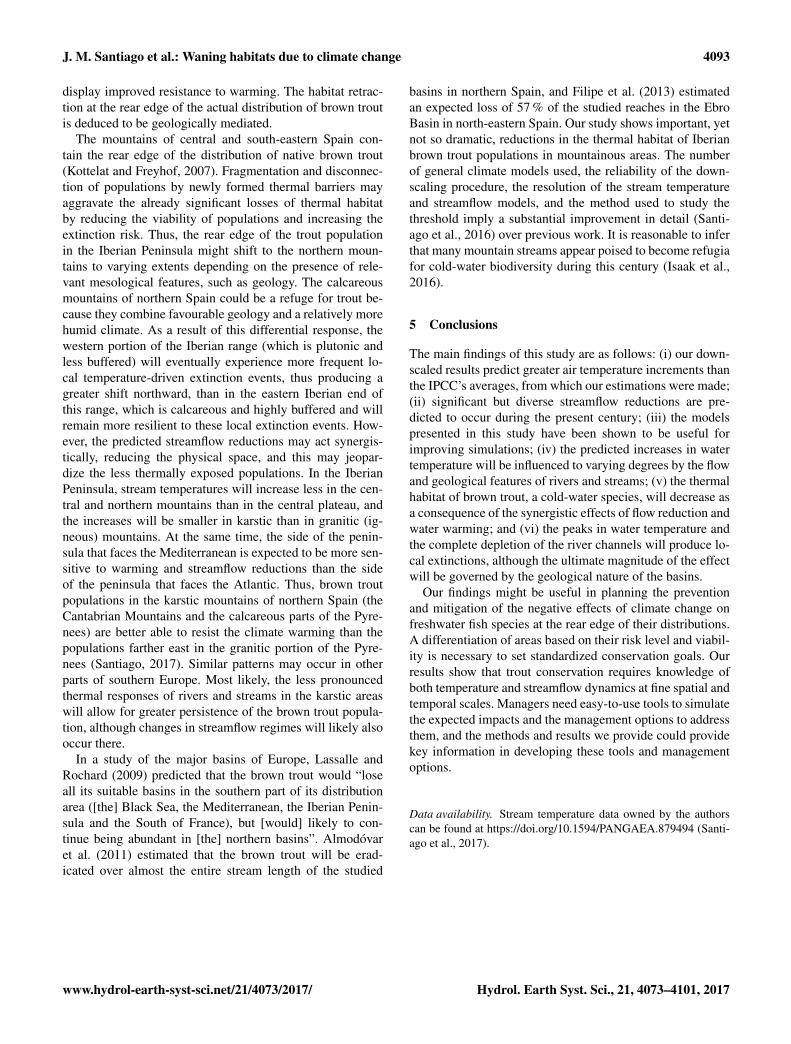
J. M. Santiago et al.: Waning habitats due to climate change 4093
display improved resistance to warming. The habitat retrac-tion at the rear edge of the actual distribution of brown troutis deduced to be geologically mediated.
The mountains of central and south-eastern Spain con-tain the rear edge of the distribution of native brown trout(Kottelat and Freyhof, 2007). Fragmentation and disconnec-tion of populations by newly formed thermal barriers mayaggravate the already significant losses of thermal habitatby reducing the viability of populations and increasing theextinction risk. Thus, the rear edge of the trout populationin the Iberian Peninsula might shift to the northern moun-tains to varying extents depending on the presence of rele-vant mesological features, such as geology. The calcareousmountains of northern Spain could be a refuge for trout be-cause they combine favourable geology and a relatively morehumid climate. As a result of this differential response, thewestern portion of the Iberian range (which is plutonic andless buffered) will eventually experience more frequent lo-cal temperature-driven extinction events, thus producing agreater shift northward, than in the eastern Iberian end ofthis range, which is calcareous and highly buffered and willremain more resilient to these local extinction events. How-ever, the predicted streamflow reductions may act synergis-tically, reducing the physical space, and this may jeopar-dize the less thermally exposed populations. In the IberianPeninsula, stream temperatures will increase less in the cen-tral and northern mountains than in the central plateau, andthe increases will be smaller in karstic than in granitic (ig-neous) mountains. At the same time, the side of the penin-sula that faces the Mediterranean is expected to be more sen-sitive to warming and streamflow reductions than the sideof the peninsula that faces the Atlantic. Thus, brown troutpopulations in the karstic mountains of northern Spain (theCantabrian Mountains and the calcareous parts of the Pyre-nees) are better able to resist the climate warming than thepopulations farther east in the granitic portion of the Pyre-nees (Santiago, 2017). Similar patterns may occur in otherparts of southern Europe. Most likely, the less pronouncedthermal responses of rivers and streams in the karstic areaswill allow for greater persistence of the brown trout popula-tion, although changes in streamflow regimes will likely alsooccur there.
In a study of the major basins of Europe, Lassalle andRochard (2009) predicted that the brown trout would “loseall its suitable basins in the southern part of its distributionarea ([the] Black Sea, the Mediterranean, the Iberian Penin-sula and the South of France), but [would] likely to con-tinue being abundant in [the] northern basins”. Almodóvaret al. (2011) estimated that the brown trout will be erad-icated over almost the entire stream length of the studied
basins in northern Spain, and Filipe et al. (2013) estimatedan expected loss of 57 % of the studied reaches in the EbroBasin in north-eastern Spain. Our study shows important, yetnot so dramatic, reductions in the thermal habitat of Iberianbrown trout populations in mountainous areas. The numberof general climate models used, the reliability of the down-scaling procedure, the resolution of the stream temperatureand streamflow models, and the method used to study thethreshold imply a substantial improvement in detail (Santi-ago et al., 2016) over previous work. It is reasonable to inferthat many mountain streams appear poised to become refugiafor cold-water biodiversity during this century (Isaak et al.,2016).
5 Conclusions
The main findings of this study are as follows: (i) our down-scaled results predict greater air temperature increments thanthe IPCC’s averages, from which our estimations were made;(ii) significant but diverse streamflow reductions are pre-dicted to occur during the present century; (iii) the modelspresented in this study have been shown to be useful forimproving simulations; (iv) the predicted increases in watertemperature will be influenced to varying degrees by the flowand geological features of rivers and streams; (v) the thermalhabitat of brown trout, a cold-water species, will decrease asa consequence of the synergistic effects of flow reduction andwater warming; and (vi) the peaks in water temperature andthe complete depletion of the river channels will produce lo-cal extinctions, although the ultimate magnitude of the effectwill be governed by the geological nature of the basins.
Our findings might be useful in planning the preventionand mitigation of the negative effects of climate change onfreshwater fish species at the rear edge of their distributions.A differentiation of areas based on their risk level and viabil-ity is necessary to set standardized conservation goals. Ourresults show that trout conservation requires knowledge ofboth temperature and streamflow dynamics at fine spatial andtemporal scales. Managers need easy-to-use tools to simulatethe expected impacts and the management options to addressthem, and the methods and results we provide could providekey information in developing these tools and managementoptions.
Data availability. Stream temperature data owned by the authorscan be found at https://doi.org/10.1594/PANGAEA.879494 (Santi-ago et al., 2017).
www.hydrol-earth-syst-sci.net/21/4073/2017/ Hydrol. Earth Syst. Sci., 21, 4073–4101, 2017

4094 J. M. Santiago et al.: Waning habitats due to climate change
Appendix A: Table of symbols and abbreviations(alphabetically ordered)
Symbol/abbreviation Meaning
a.c. agglomerative coefficientAEMET Spanish Meteorological AgencyAIC Akaike information criterionα maximum stream temperatureAR5 Fifth Assessment Report of the IPCCβ air temperature at which the rate of change of the stream temperature with respect to the air
temperature is a maximumBIC Bayesian information criterionCMIP5 Fifth Coupled Model Intercomparison ProjectDAT total days above the threshold per yearδ maximum rate at τ .1Ta 1-day variation in the daily mean air temperature1Tmax increments of the annual averages of the daily maximum stream temperature1Tmean increments of the annual averages of the daily mean stream temperature1Tmin increments of the annual averages of the daily minimum stream temperatureDEM digital elevation modelDMAT daily mean air temperatureDMST daily mean steam temperatureECDF empirical cumulative distribution functionsγ rate of change at βH-2050 year horizon 2050H-2099 year horizon 2099IGN National Geographic Institute of the Spanish GovernmentIPCC Intergovernmental Panel on Climate Changeλ represents the resistance of DMST to change with respect to the 1-day variation in DMAT (1Ta)M5 machine learning techniqueMCDAT maximum consecutive days above the threshold per yearµ minimum stream temperatureNSE Nash–Sutcliffe efficiencyω maximum observable variation in stream temperature due to the flow differencePACF partial autocorrelation functionQ10 10th percentile of flowQmax maximum flowQmean mean flowQmin minimum flowRCP4.5 Representative Concentration Pathway 4.5RCP8.5 Representative Concentration Pathway 8.5RSE residual standard errorTa air temperatureTAT≥ 7 frequency of events of seven or more consecutive days above the threshold per yearτ low value at which the rate of change of the stream temperature with respect to the flow
is a maximumTs stream temperature
Hydrol. Earth Syst. Sci., 21, 4073–4101, 2017 www.hydrol-earth-syst-sci.net/21/4073/2017/

J. M. Santiago et al.: Waning habitats due to climate change 4095
Appendix B: Uncertainty
In science, and particularly in hydrological studies, the un-certainty is a matter which requires special attention, and ithas led us to include a synthesis of our approach to this prob-lem in this appendix. The uncertainty analysis is a necessarystep in assessing the risk level in the applicability of a model(Pappenberger and Beven, 2006). Our aim was to study theviability of the brown trout populations, and we modelledthe flow and the stream temperature for this purpose. Froma conceptual point of view our approaches were consistentwith it.
On data inputs to build the models, uncertainties and in-consistencies are a habitual issue (Juston et al., 2013). Themeteorological and hydrological services subject data to theirown quality controls but systematic error cannot always becompletely controlled (Beven and Westerberg, 2011; McMil-lan et al., 2012). For this reason, in addition, we tested theinput data seeking inconsistencies.
The modelling of the river reaches as one-dimensional el-ements implies a simplification of the fluvial ecosystem thatis generally accepted at this scale (e.g. Viganò et al., 2015;Ahmed and Tsanis, 2016), especially for ecological purposes(e.g. Caiola et al., 2014). Nevertheless, the size of the riversunder study made little or nothing relevant the variations inwidth and depth (it was verified in the field).
Regarding the parameterization of the models, cross-validation was used to evaluate the uncertainty in these pro-cess, and indicators such as the NSE (for hydrological andthermal models), the deviance and the RSE (for thermal mod-els) were calculated. In the case of the thermal model, thefunctions of distribution of the parameters of the model werebuilt by non-parametric bootstrap, and the mean values werechosen as the most proficient estimators. As results show, pa-
rameters tell us about the functional behaviour of catchments(particularly on the effects of the catchments geology on thestreams temperature) and this might improve predictions inungauged basins by better controlling uncertainty (Juston etal., 2013).
Once the models were constructed, It was verified thatthe overlaps of the ranges of the model input variables andthe ranges of the outputs were significant (p < 0.05). Thenon-overlapping zones affected, on the one hand, infrequentevents (great floods) and the extreme temperature zone (zoneof extrapolation), being the last one the scope in which weexpected to work. However, the weakness of the hydrologi-cal model in the flood zone should be considered for otherapplications and developments of the model. The hydrologi-cal model given us sufficient and relevant information sinceits possible weak points (extrapolation in the floods assess-ment) did not affect our goal: we focused on central trendsand minimum values, and they were solidly represented inthe samples and in the simulations.
As said, the inherent uncertainty of the climate predictionsaccording to the scenarios RCP4.5 and RCP8.5 was attenu-ated by means of the ensemble technique, showing the dis-persion of the results by mean of the percentiles in Figs. S1to S24 (in the Supplement). Beven (2011) exposed his legit-imate concerns on the credibility of climate models whichfail when are compared with the control period and, conse-quently, we used ERA-40 reanalysis to control this source ofbias with excellent results.
There was a time dependence between the errors of themodel and the scope of the prediction, but these errors wereonly important in the zone of high temperature and low flow,as expected by the physical nature of the climatic variables.Moreover, this is the behaviour of the variables that was ourintention to evaluate.
www.hydrol-earth-syst-sci.net/21/4073/2017/ Hydrol. Earth Syst. Sci., 21, 4073–4101, 2017
4096 J. M. Santiago et al.: Waning habitats due to climate change
The Supplement related to this article is availableonline at https://doi.org/10.5194/hess-21-4073-2017-supplement.
Competing interests. The authors declare that they have no conflictof interest.
Acknowledgements. We are grateful to the Consejería de MedioAmbiente y O.T. of the Government of Castilla y León, especiallyto Mariano Anchuelo, Fabián Mateo and the forest ranger team ofNavafría. Also, we are indebted to the Sierra of Guadarrama Na-tional Park staff, and especially with Juan Bielva and Ángel Rubiofor the temperature data of Lozoya stream. Juan Diego Alcaraz isthe author of the temperature data of the Ebrón Basin. Valérie Ouel-let and two anonymous referees provided valuable comments thatsubstantially improved the original manuscript. The World ClimateResearch Programme’s Working Group on Coupled Modelling isresponsible for the 5th Coupled Model Intercomparison Project,and we thank the climate modelling groups for producing and mak-ing available their model output. Climate change study was partiallyfunded by the Ministerio de Agricultura, Alimentación y MedioAmbiente of Spain through the Fundación para la Investigación delClima (http://www.ficlima.org/); by the European Union, DG forEnvironment (DURERO project. C1.3913442); by the Ministeriode Economía y Competitividad of Spain (IMPADAPT projectCGL2013-48424-C2-1-R); and by FEDER funds of the EuropeanCommission.
Edited by: Jan SeibertReviewed by: Valerie Ouellet and two anonymous referees
References
Ahmed, S. and Tsanis, I.: Hydrologic and Hydraulic Impact of Cli-mate Change on Lake Ontario Tributary, Am. J. Water Resour.,4, 1–15, https://doi.org/10.12691/ajwr-4-1-1, 2016.
Allen, K. R.: Comparison of the Growth Rate of BrownTrout (Salmo trutta) in a New Zealand Stream with Ex-perimental Fish in Britain, J. Anim. Ecol., 54, 487–495,https://doi.org/10.2307/4493, 1985.
Almodóvar, A., Nicola, G. G., Ayllón, D., and Elvira, B.:Global warming threatens the persistence of Mediter-ranean brown trout, Glob. Change Biol., 18, 1549–1560,https://doi.org/10.1111/j.1365-2486.2011.02608.x, 2011.
Angilletta Jr., M. J.: Thermal Adaptation: A Theoretical and Empir-ical Synthesis, Oxford University Press, New York, USA, 2009.
Arismendi, I., Safeeq, M., Dunham, J. B., and Johnson, S. L.:Can air temperature be used to project influences of climatechange on stream temperature?, Environ. Res. Lett., 9, 084015,https://doi.org/10.1088/1748-9326/9/8/084015, 2014.
Ayllón, D., Railsback, S. F., Vincenzi, S., Groeneveld, J., Almod-óvar, A., and Grimm, V.: InSTREAM-Gen: Modelling eco-evolutionary dynamics of trout populations under anthro-pogenic environmental change, Ecol. Model., 326, 36–53,https://doi.org/10.1016/j.ecolmodel.2015.07.026, 2016.
Beer, W. N. and Anderson, J. J.: Sensitivity of salmonidfreshwater life history in western US streams to futureclimate conditions, Glob. Change Biol., 19, 2547–2556,https://doi.org/10.1111/gcb.12242, 2013.
Bennett, N. D., Croke, B. F. W., Guariso, G., Guillaume, J. H. A.,Hamilton, S. H., Jakeman, A. J., Marsili-Libelli, S., Newham, L.T. H., Norton, J. P., Perrin, C., Pierce, S. A., Robson, B., Sep-pelt, R., Voinov, A. A., Fath, B. D., and Andreassian, V.: Charac-terising performance of environmental models, Environ. Modell.Softw., 40, 1–20, https://doi.org/10.1016/j.envsoft.2012.09.011,2013.
Beven, K.: I believe in climate change but how precautionary dowe need to be in planning for the future?, Hydrol. Process., 25,1517–1520, https://doi.org/10.1002/hyp.7939, 2011.
Beven, K. and Westerberg, I.: On red herrings and real herrings:disinformation and information in hydrological inference, Hy-drol. Process., 25, 1676–1680, https://doi.org/10.1002/hyp.7963,2011.
Bogan, T., Mohseni, O., and Stefan, H. G.: Stream temperature-equilibrium temperature relationship, Water Resour. Res., 39,1245, https://doi.org/10.1029/2003WR002034, 2003.
Borra, S. and Di Ciaccio, A.: Measuring the prediction error.A comparison of cross-validation, bootstrap and covariancepenalty methods, Comput. Stat. Data An., 54, 2976–2989,https://doi.org/10.1016/j.csda.2010.03.004, 2010.
Breiman, L.: Random forests, Mach. Learn., 45, 5–32,https://doi.org/10.1023/A:1010933404324, 2001.
Brewitt, K. S. and Danner, E. M.: Spatio-temporal temperature vari-ation influences juvenile steelhead (Oncorhynchus mykiss) use ofthermal refuges, Ecosphere, 5, 92, https://doi.org/10.1890/ES14-00036.1, 2014.
Bustillo, V., Moatar, F., Ducharne, A., Thiéry, D., and Poirel, A.:A multimodel comparison for assessing water temperatures un-der changing climate conditions via the equilibrium tempera-ture concept: case study of the Middle Loire River, France, Hy-drol. Process., 28, 1507–1524, https://doi.org/10.1002/hyp.9683,2013.
Caiola, N., Ibáñez, C., Verdú, J., and Munné, A.: Effectsof flow regulation on the establishment of alien fishspecies: A community structure approach to biological val-idation of environmental flows, Ecol. Indic., 45, 598–604,https://doi.org/10.1016/j.ecolind.2014.05.012, 2014.
Caissie, D.: The thermal regime of rivers: a review, Fresh-water Biol., 51, 1389–1406, https://doi.org/10.1111/j.1365-2427.2006.01597.x, 2006.
Ceballos-Barbancho, A., Morán-Tejeda, E., Luego-Ugidos, M. A.,and Llorente-Pinto, J. M.: Water resources and environmentalchange in a Mediterranean environment: The south-west sec-tor of the Duero river basin (Spain), J. Hydrol., 351, 126–138,https://doi.org/10.1016/j.jhydrol.2007.12.004, 2008.
Chen, D., Hu, M., Guo, Y., and Dahlgren, R.A.: Changes in riverwater temperature between 1980–2012 in Yongan watershed,eastern China: magnitude, drivers and models, J. Hydrol., 533,191–199, https://doi.org/10.1016/j.jhydrol.2015.12.005, 2016.
Chessman, B. C.: Climatic changes and 13-year trends instream macroinvertebrate assemblages in New SouthWales, Australia, Glob. Change Biol., 15, 2791–2802,https://doi.org/10.1111/j.1365-2486.2008.01840.x, 2009.
Hydrol. Earth Syst. Sci., 21, 4073–4101, 2017 www.hydrol-earth-syst-sci.net/21/4073/2017/
J. M. Santiago et al.: Waning habitats due to climate change 4097
Chilton, J.: Groundwater, in: Water quality assessments: A guide tothe use of biota, sediments and water in environmental monitor-ing, 2nd ed., edited by: Chapman, D. E. and Spon, F. N., London,UK, 413–510, 1996.
Colchen, T., Teletchea, F., Fontaine, P., and Pasquet, A.:Temperature modifies activity, inter-individual relationshipsand group structure in fish, Curr. Zool., 63, 175–183,https://doi.org/10.1093/cz/zow048, 2017.
Comte, L., Buisson, L., Daufresne, M., and Grenouillet, G.:Climate-induced changes in the distribution of freshwater fish:observed and predicted trends, Freshwater Biol., 58, 625–639,https://doi.org/10.1111/fwb.12081, 2013.
Daigle, A., Jeong, D. I., and Lapointe, M. F.: Climate changeand resilience of tributary thermal refugia for salmonids ineastern Canadian rivers, Hydrolog. Sci. J., 60, 1044–1063,https://doi.org/10.1080/02626667.2014.898121, 2014.
De’ath, G. and Fabricius, K. E.: Classification and regression trees:a powerful yet simple technique for ecological data analysis,Ecology, 81, 3178–3192, https://doi.org/10.2307/177409, 2000.
DeWeber, J. T. and Wagner, T.: Predicting Brook trout oc-currence in stream reaches throughout their native range inthe Eastern United States, T. Am. Fish. Soc., 144, 11–24,https://doi.org/10.1080/00028487.2014.963256, 2015.
Eby, L. A., Helmy, O., Holsinger, L. M., and Young, M. K.: Evi-dence of climate-induced range contractions in bull trout Salveli-nus confluentus in a Rocky Mountain watershed, U.S.A., PLoSONE, 9, e98812, https://doi.org/10.1371/journal.pone.0098812,2014.
Edinger, J. E., Duttweiler, D. W., and Geyer, J. C.: The response ofwater temperatures to meteorological conditions, Water Resour.Res., 4, 1137–1143, https://doi.org/10.1029/WR004i005p01137,1968.
Elith, J. and Leathwick, J. R.: Species distribution mod-els: Ecological explanation and prediction across spaceand time, Annu. Rev. Ecol. Evol. S., 40, 677–697,https://doi.org/10.1146/annurev.ecolsys.110308.120159, 2009.
Elliott, J. M.: Some aspects of thermal stress on freshwater teleosts,in: Stress and Fish, edited by: Pickering, A. D., Academic Press,London, UK, 209–245, 1981.
Elliott, J. M.: Pools as refugia for brown trout during twosummer droughts: trout responses to thermal and oxygenstress, J. Fish Biol., 56, 938–948, https://doi.org/10.1111/j.1095-8649.2000.tb00883.x, 2000.
Elliott, J. M. and Allonby, J. D.: An experimental study of onto-genetic and seasonal changes in the temperature preferences ofunfed and fed brown trout, Salmo trutta, Freshwater Biol., 58,1840–1848, https://doi.org/10.1111/fwb.12173, 2013.
Elliott, J. M. and Elliott, J. A.: Temperature requirements of At-lantic salmon Salmo salar, Brown trout Salmo trutta and Arcticcharr Salvelinus alpinus: predicting the effects of climate change,J. Fish Biol., 77, 1793–1817, https://doi.org/10.1111/j.1095-8649.2010.02762.x, 2010.
Elliott, J. M., Hurley, M. A., and Fryer, J.: A new, improved growthmodel for brown trout, Salmo trutta, Funct. Ecol., 9, 290–298,https://doi.org/10.2307/2390576, 1995.
European Environment Agency: CLC2006 technical guidelines.Technical report No. 17/2007, Publications Office, Luxembourg,https://doi.org/10.2800/12134, 2007.
Fey, S. B. and Herren, C. M.: Temperature-mediated bi-otic interactions influence enemy release of non-nativespecies in warming environments, Ecology, 95, 2246–2256,https://doi.org/10.1890/13-1799.1, 2014.
Fielding, A. H.: An introduction to machine learning methods. In:Machine Learning Methods for Ecological Applications, editedby: Fielding, A. H., Kluwer, Boston, USA, 1–35, 1999.
Filipe, A. F., Markovic, D., Pletterbauer, F., Tisseuil, C., DeWever, A., Schmutz, S., Bonada, N., and Freyhof, J: Fore-casting fish distribution along stream networks: brown trout(Salmo trutta) in Europe, Divers. Distrib., 19, 1059–1071,https://doi.org/10.1111/ddi.12086, 2013.
Forseth, T. and Jonsson, B.: The growth and food ration of pis-civorous brown trout (Salmo trutta), Funct. Ecol., 8, 171–177,https://doi.org/10.2307/2389900, 1994.
Forseth, T., Larsson, S., Jensen, A. J., Jonsson, B., Näslund, I.,and Berglund, I.: Thermal growth performance of juvenile browntrout Salmo trutta?: no support for thermal adaptation hypothe-ses, J. Fish Biol., 74, 133–149, https://doi.org/10.1111/j.1095-8649.2008.02119.x, 2009.
Fukuda, S., De Baets, B., Waegeman, W., Verwaeren, J., and Mou-ton, A. M.: Habitat prediction and knowledge extraction forspawning European grayling (Thymallus thymallus L.) using abroad range of species distribution models, Environ. Modell.Softw., 47, 1–6, https://doi.org/10.1016/j.envsoft.2013.04.005,2013.
Garner, G., Van Loon, A. F., Prudhomme, C., and Hannah, D. M.:Hydroclimatology of extreme river flows, Freshwater Biol., 60,2461–2476, https://doi.org/10.1111/fwb.12667, 2015.
Gordon, N. D., McMahon, T. A., Finlayson, B. L., Gippel, C. J., andNathan, R. J.: Stream hydrology. An introduction for ecologists,2nd ed., John Wiley and Sons, Chichester, UK, 2004.
Gortázar, J., García de Jalón, D., Alonso-González, C., Vizcaíno,P., Baeza, D., and Marchamalo, M.: Spawning period of a south-ern brown trout population in a highly unpredictable stream,Ecol. Freshw. Fish, 16, 515–527, https://doi.org/10.1111/j.1600-0633.2007.00246.x, 2007.
Goyer, K., Bertolo, A., Pépino, M., and Magnan, P.: Ef-fects of lake warming on behavioural thermoregulatory tac-tics in a cold-water stenothermic fish, PLoS ONE, 9, e92514,https://doi.org/10.1371/journal.pone.0092514, 2014.
Grande, M. and Andersen, S.: Critical Thermal Maximafor Young Salmonids, J. Freshwater Ecol., 6, 275–279,https://doi.org/10.1080/02705060.1991.9665304, 1991.
Haines, A. T., Finlayson, B. L., and McMahon, T. A.: A globalclassification of river regimes, Appl. Geogr., 8, 255–272,https://doi.org/10.1016/0143-6228(88)90035-5, 1988.
Hampe, A. and Petit, R. J.: Conserving biodiversity under cli-mate change: the rear edge mattersm Ecol. Lett., 8, 461–467,https://doi.org/10.1111/j.1461-0248.2005.00739.x, 2005.
Hari, R. E., Livingstone, D. M., Siber, R., Burkhardt-Holm,P., and Guettinger, H.: Consequences of climatic changefor water temperature and brown trout populations inAlpine rivers and streams, Glob. Change Biol., 12, 10–26,https://doi.org/10.1111/j.1365-2486.2005.001051.x, 2006.
Hein, C. L., Ohlund, G., and Englund, G.: Fish introduc-tions reveal the temperature dependence of species in-teractions, P. Roy. Soc. B-Biol. Sci., 281, 20132641,https://doi.org/10.1098/rspb.2013.2641, 2013.
www.hydrol-earth-syst-sci.net/21/4073/2017/ Hydrol. Earth Syst. Sci., 21, 4073–4101, 2017

4098 J. M. Santiago et al.: Waning habitats due to climate change
Hettiarachchi, P., Hall, M. J., and Minns, A. W.: The extrapolationof artificial neural networks for the modelling of rainfall–runoffrelationships, J. Hydroinform., 7, 291–296, 2005.
IGME: Mapa de Litologías de España 1 : 1 000 000, Madrid, Spain,available at: http://mapas.igme.es/gis/rest/services/Cartografia_Geologica/IGME_Litologias_1M/MapServer (last access:15 February 2016), 2015.
IPCC: Climate Change 2013. The Physical Science Basis. Work-ing Group I Contribution to the Fifth Assessment Report of theIntergovernmental Panel on Climate Change, edited by: Stocker,T. F., Qin, D., Plattner, G.-K., Tignor, M. M. B., Allen, S. K.,Boschung, J., Nauels, A., Xia, Y., Bex, V., and Midgley, P. M.,Cambridge University Press, Cambridge, UK, 2013.
Isaak, D. J., Young, M. K., Luce, C. H., Hostetler S. W.,Wenger, S. J., Peterson, E. E., Ver Hoef, J. M., Groce, M.C., Horan, D. L., and Nagel, D. E.: Slow climate velocitiesof mountain streams portend their role as refugia for cold-water biodiversity, P. Natl. Acad. Sci. USA, 113, 4374–4379,https://doi.org/10.1073/pnas.1522429113, 2016.
Jeffries, K. M., Hinch, S. G., Martins, E. G., Clark, T. D.,Lotto, A. G., Patterson, D. A., Cooke, S. J., Farrell, A. P.,and Miller, K. M.: Sex and proximity to reproductive matu-rity influence the survival, final maturation, and blood physiol-ogy of Pacific salmon when exposed to high temperature dur-ing a simulated migration, Physiol. Biochem. Zool., 85, 62–73,https://doi.org/10.1086/663770, 2012.
Jonsson, B. and Jonsson, N.: A review of the likely effects ofclimate change on anadromous Atlantic salmon Salmo salarand brown trout Salmo trutta, with particular reference towater temperature and flow, J. Fish Biol., 75, 2381–2447,https://doi.org/10.1111/j.1095-8649.2009.02380.x, 2009.
Junker, J., Heimann, F. U. M., Hauer, C., Turowski, J. M., Rick-enmann, D., Zappa, M., and Peter, A.: Assessing the impact ofclimate change on brown trout (Salmo trutta fario) recruitment,Hydrobiologia, 751, 1–21, https://doi.org/10.1007/s10750-014-2073-4, 2015.
Juston, J. M., Kauffeldt, A., Montano, B. Q., Seibert, J., Beven,K. J., and Westerberg, I. K.: Smiling in the rain: Seven reasonsto be positive about uncertainty in hydrological modelling, Hy-drol. Process., 27, 1117–1122, https://doi.org/10.1002/hyp.9625,2013.
Kaufman, L. and Rousseeuw, P. J.: Finding Groups in Data: AnIntroduction to Cluster Analysis. John Wiley & Sons, Hobo-ken, New Jersey, USA, https://doi.org/10.1002/9780470316801,2005.
Kaushal, S. S., Likens, G. E., Jaworski, N. A., Pace, M. L., Sides, A.M., Seekell, D., Belt, K. T., Secor, D. H., and Wingate, R.: Risingstream and river temperatures in the United States, Front. Ecol.Environ., 8, 461–466, https://doi.org/10.1890/090037, 2010.
Kittler, J.: Feature set search algorithms, in: Pattern Recognitionand Signal Processing, edited by: Chen, C. H., Sijthoff and No-ordhoff, Alphen aan den Rijn, the Netherlands, 41–60, 1978.
Kottelat, M. and Freyhof, J.: Handbook of European freshwaterfishes, Kottelat, Cornol, Switzerland and Freyhof, Berlin, Ger-many, 2007.
Kuhn, M., Weston, S., Keefer, C., and Coulter, N.: Cubist: Rule-and Instance-Based Regression Modeling – C code for Cubistby Ross Quinlan, R package, version 0.0.18, CRAN R-Projectpackage, version 0.0.18, CRAN R-Project, available at: https://
cran.r-project.org/package=Cubist (last access: 15 August 2015),2014.
Kurylyk, B. L., Bourque, C. P.-A., and MacQuarrie, K. T. B.: Po-tential surface temperature and shallow groundwater temperatureresponse to climate change: an example from a small forestedcatchment in east-central New Brunswick (Canada), Hydrol.Earth Syst. Sci., 17, 2701–2716, https://doi.org/10.5194/hess-17-2701-2013, 2013.
Kurylyk, B. L., MacQuarrie, K. T. B., Caissie, D., and McKenzie,J. M.: Shallow groundwater thermal sensitivity to climate changeand land cover disturbances: derivation of analytical expressionsand implications for stream temperature modeling, Hydrol. EarthSyst. Sci., 19, 2469–2489, https://doi.org/10.5194/hess-19-2469-2015, 2015.
Lahnsteiner, F. and Leitner, S.: Effect of temperature on gametoge-nesis and gamete quality in Brown trout, Salmo trutta, J. Exp.Zool. Part A, 319, 138–148, https://doi.org/10.1002/jez.1779,2013.
Larios-López, J. E., Tierno de Figueroa, J. M., Galiana-García,M., Gortázar, J., and Alonso, C.: Extended spawning in browntrout (Salmo trutta) populations from the Southern Iberian Penin-sula: the role of climate variability, J. Limnol., 74, 394–402,https://doi.org/10.4081/jlimnol.2015.1089, 2015.
Lassalle, G. and Rochard, E.: Impact of twenty-first century cli-mate change on diadromous fish spread over Europe, NorthAfrica and the Middle East, Glob. Change Biol., 15, 1072–1089,https://doi.org/10.1111/j.1365-2486.2008.01794.x, 2009.
Leppi, J. C., DeLuca, T. H., Harrar, S. W.. and Running, S. W.:Impacts of climate change on August stream discharge in theCentral-Rocky Mountains, Climatic Change, 112, 997–1014,https://doi.org/10.1007/s10584-011-0235-1, 2012.
Liu, R. and Singh, K.: Moving blocks jackknife and bootstrap cap-ture weak dependence, in: Exploring the Limits of Bootstrap,edited by: LePage, R. and Billard, L., John Wiley and Sons, NewYork, USA, 225–248, 1992.
Lobón-Cerviá, J. and Rincón, P. A.: Field assessment of the influ-ence of temperature on growth rate in a brown trout population,T. Am. Fish. Soc., 127, 718–728, https://doi.org/10.1577/1548-8659(1998)127<0718:FAOTIO>2.0.CO;2, 1998.
Lobón-Cerviá, J. and Mortensen, E.: Population size in stream-living juveniles of lake-migratory brown trout Salmo truttaL.: the importance of stream discharge and temperature,Ecol. Freshw. Fish, 14, 394–401, https://doi.org/10.1111/j.1600-0633.2005.00111.x, 2005.
Lobón-Cerviá, J. and Rincón, P. A.: Environmental determinantsof recruitment and their influence on the population dynamicsof stream-living brown trout Salmo trutta, Oikos, 105, 641–646,https://doi.org/10.1111/j.0030-1299.2004.12989.x, 2004.
Loinaz, M. C., Davidsen, H. K., Butts, M., and Bauer-Gottwein, P.: Integrated flow and temperature model-ing at the catchment scale, J. Hydrol., 495, 238–251,https://doi.org/10.1016/j.jhydrol.2013.04.039, 2013.
Lorenzo-Lacruz, J., Vicente-Serrano, S. M., López-Moreno, J.I., Morán-Tejeda, E., and Zabalza, J.: Recent trends inIberian streamflows (1945–2005), J. Hydrol., 414–415, 463–475,https://doi.org/10.1016/j.jhydrol.2011.11.023, 2012.
Luce, C. H. and Holden, Z. A.: Declining annual stream-flow distributions in the Pacific Northwest United
Hydrol. Earth Syst. Sci., 21, 4073–4101, 2017 www.hydrol-earth-syst-sci.net/21/4073/2017/
J. M. Santiago et al.: Waning habitats due to climate change 4099
States, 1948–2006, Geophys. Res. Lett., 36, L16401,https://doi.org/10.1029/2009GL039407, 2009.
Maechler, M.: Cluster analysis extended, Rousseeuw et al., R pack-age, version 1.14.4, CRAN R-Project, available at: https://cran.r-project.org/package=cluster (last access: 15 August 2015),2013.
Magnuson, J. J. and Destasio, B. T.: Thermal niche of fishes andglobal warming, in: Global Warming: Implications for Freshwa-ter and Marine Fish, edited by: Wood, C. M. and McDonald,D. G., Cambridge University Press, Cambridge, UK, 377–407,1997.
Magnuson, J. J., Crowder, L. B., and Medvick, P. A.: Temper-ature as an Ecological Resource, Am. Zool., 19, 331–343,https://doi.org/10.1093/icb/19.1.331, 1979.
McCuen, R. H.: Hydrologic analysis and design, 2nd ed., PrenticeHall, New Jersey, USA, 1998.
McMillan, H., Krueger, K., and Freer, J.: Benchmarking ob-servational uncertainties for hydrology: Rainfall, river dis-charge and water quality, Hydrol. Process., 26, 4078–4111,https://doi.org/10.1002/hyp.9384, 2012.
Meshcheryakova, O. V., Churova, M. V., Veselov, A. E., andNemova, N. N.: Activities of cytochrome c oxidase and mi-tochondrial lactate dehydrogenase isozymes and Cox1, Cox2,Cox4, and Cox6 gene subunit expression in cold adaptationof Salmo trutta L., Russ. J. Bioorganic Chem., 42, 162–169,https://doi.org/10.1134/S1068162016010106, 2016.
Milly, P. C. D., Dunne, K. A., and Vecchia, A. V.: Global pattern oftrends in streamflow and water availability in a changing climate,Nature, 438, 347–350, https://doi.org/10.1038/nature04312,2005.
Mohseni, O. and Stefan, H.: Stream temperature/air temperature re-lationship: a physical interpretation, J. Hydrol., 218, 128–141,https://doi.org/10.1016/S0022-1694(99)00034-7, 1999.
Mohseni, O., Stefan, H. G., and Eriksson, T. R.: A nonlinear regres-sion model for weekly stream temperatures, Water Resour. Res.,34, 2685–2692, https://doi.org/10.1029/98WR01877, 1998.
Monjo, R., Caselles, V., and Chust, G.: Probabilistic cor-rection of RCM precipitation in the Basque Country(Northern Spain), Theor. Appl. Climatol., 117, 317–329,https://doi.org/10.1007/s00704-013-1008-8, 2014.
Morán-Tejeda, E., Lorenzo-Lacruz, J., López-Moreno, J. I., Rah-man, K., and Beniston, M.: Streamflow timing of mountain riversin Spain: Recent changes and future projections, J. Hydrol., 517,1114–1127, https://doi.org/10.1016/j.jhydrol.2014.06.053, 2014.
Muñoz-Mas, R., López-Nicolás, A., Martínez-Capel, F., andPulido-Velázquez, M.: Shifts in the suitable habitat avail-able for brown trout (Salmo trutta L.) under short-term cli-mate change scenarios, Sci. Total Environ., 544, 686–700,https://doi.org/10.1016/j.scitotenv.2015.11.147, 2016.
Nakicenovic, N., Alcamo, J., Davis, G., de Vries, H. J. M., Fen-hann, J., Gaffin, S., Gregory, K., Grubler, A., Jung, T. Y., Kram,T., La Rovere, E. L., Michaelis, L., Mori, S., Morita, T., Papper,W., Pitcher, H., Price, L., Riahi, K., Roehrl, A., Rogner, H.-H.,Sankovski, A., Schlesinger, M., Shukla, P., Smith, S., Swart, R.,van Rooijen, S., Victor, N., and Dadi, Z.: Emissions Scenarios:A Special Report of Working Group III of the Intergovernmen-tal Panel on Climate Change, Cambridge University Press, Cam-bridge, UK, 2000.
Nash, J. E. and Sutcliffe, J. V.: River flow forecasting through con-ceptual models part I – A discussion of principles, J. Hydrol., 10,282–290, https://doi.org/10.1016/0022-1694(70)90255-6, 1970.
Neumann, D. W., Rajagopalan, B., and Zagona, E. A.: Regres-sion model for daily maximum stream temperature, J. Envi-ron. Eng., 129, 667–674, https://doi.org/10.1061/(ASCE)0733-9372(2003)129:7(667), 2003.
Ojanguren, A. F., Reyes-Gavilán, F. G. and Braña, F.: Ther-mal sensitivity of growth, food intake and activity ofjuvenile brown trout, J. Therm. Biol., 26, 165–170,https://doi.org/10.1016/S0306-4565(00)00038-3, 2001.
Orr, H. G., Simpson, G. L., des Clers, S., Watts, G., Hughes, M.,Hannaford, J., Dunbar, M. J., Laizé, C. L. R., Wilby, R. L., Bat-tarbee, R. W., and Evans, R.: Detecting changing river temper-atures in England and Wales, Hydrol. Process., 29, 752–766,https://doi.org/10.1002/hyp.10181, 2015.
Pappenberger, F. and Beven, K. J.: Ignorance is bliss: 7 reasonsnot to use uncertainty analysis, Water Resour. Res., 42, W05302,https://doi.org/10.1029/2005WR004820, 2006.
Pépino, M., Goyer, K., and Magnan, P.: Heat transfer in fish: areshort excursions between habitats a thermoregulatory behaviourto exploit resources in an unfavourable thermal environment?, J.Exp. Biol., 218, 3461–3467, https://doi.org/10.1242/jeb.126466,2015.
Piccolroaz, S., Calamita, E., Majone, B., Gallice, A., Siviglia, A.,and Toffolon, M.: Prediction of river water temperature: a com-parison between a new family of hybrid models and statisticalapproaches: Prediction of River Water Temperature, Hydrol. Pro-cess., 30, 3901–3917, https://doi.org/10.1002/hyp.10913, 2016
Pohlert, T.: Non-parametric trend tests and change-point detection,R package, version 0.1.0, CRAN R-Project, available at: https://cran.r-project.org/package=trend, last access: 10 June 2016.
Pourmokhtarian, A., Driscoll, C. T., Campbell, J. L., Hayhoe, K.,and Stoner, A. M.: The effects of climate downscaling techniqueand observational dataset on modeled ecological responses, Ecol.Appl., 26, 1321–1337, https://doi.org/10.1890/15-0745, 2016.
Quinlan, J. R.: Learning with continuous classes, in: The 5thAustralian Joint Conference on Artificial Intelligence, 16–18 November 1992, Hobart, Australia, 343–348, 1992.
Quinlan, J. R.: An overview of Cubist, available at: https://www.rulequest.com/cubist-win.html, last access: 8 June 2017.
R Core Team: R: A language and environment for statistical com-puting, R Foundation for Statistical Computing, Vienna, Aus-tria, available at: http://www.R-project.org (last access: 20 May2016), 2015.
Reynolds, W. W. and Casterlin, M. E.: Thermoregulatory behav-ior of brown trout, Salmo trutta, Hydrobiologia, 62, 79–80,https://doi.org/10.1007/BF00012567, 1979.
Ribalaygua, J., Torres, L., Pórtoles, J., Monjo, R., Gaitán, E.,and Pino, M. R.: Description and validation of a two-stepanalogue/regression downscaling method, Theor. Appl. Clima-tol., 114, 253–269, https://doi.org/10.1007/s00704-013-0836-x,2013.
Rojas, R., Feyen, L., Bianchi, A., and Dosio, A.: Assessment offuture flood hazard in Europe using a large ensemble of bias-corrected regional climate simulations, J. Geophys. Res.-Atmos.,117, D17109, https://doi.org/10.1029/2012JD017461, 2012.
Ruiz-Navarro, A., Gillingham, P. K., and Britton, J. R.: Predict-ing shifts in the climate space of freshwater fishes in Great
www.hydrol-earth-syst-sci.net/21/4073/2017/ Hydrol. Earth Syst. Sci., 21, 4073–4101, 2017

4100 J. M. Santiago et al.: Waning habitats due to climate change
Britain due to climate change, Biol. Conserv., 203, 33–42,https://doi.org/10.1016/j.biocon.2016.08.021, 2016.
Sánchez-Hernández, J. and Nunn, A.D.: Environmental changesin a Mediterranean river: implications for the fish assemblage,Ecohydrology, 9, 1439–1451, https://doi.org/10.1002/eco.1737,2016.
Santiago, J. M.: Thermal ecology of Brown trout and the climatechange challenge, in: Tilapia and Trout: Harvesting, Prevalenceand Benefits, edited by: Richardson, B., Nova Science Publish-ers, New York, USA, 79–119, 2017.
Santiago, J. M., García de Jalón, D., Alonso, C., and Solana, J.:Comportamiento térmico de dos tramos fluviales de cabeceradel sistema central: impacto del embalse de Torrecaballeros(Segovia), in: III Jornadas del Ingeniería del Agua, Valencia,Vol. 1, Marcombo, Barcelona, Spain, 153–160, 2013.
Santiago, J. M., García de Jalón, D., Alonso, C., Solana, J., Rib-alaygua, J., Pórtoles, J., and Monjo, R.: Brown trout thermalniche and climate change: expected changes in the distributionof cold-water fish in central Spain, Ecohydrology, 9, 514–528,https://doi.org/10.1002/eco.1653, 2016.
Santiago, J. M., Alonso, C., and García de Jalón, D.: Dailymean stream temperatures in Central Spain, PANGAEA,https://doi.org/10.1594/PANGAEA.879494, 2017.
Schoups, G., van de Giesen, N. C., and Savenije, H. H. G.: Modelcomplexity control for hydrologic prediction, Water Resour.Res., 44, W00B03, https://doi.org/10.1029/2008WR006836,2008.
Shortridge, J. E., Guikema, S. D., and Zaitchik, B. F.: Machinelearning methods for empirical streamflow simulation: a com-parison of model accuracy, interpretability, and uncertainty inseasonal watersheds, Hydrol. Earth Syst. Sci., 20, 2611–2628,https://doi.org/10.5194/hess-20-2611-2016, 2016.
Snyder, C. D., Hitt, N. P., and Young, J. A.: Accounting for ground-water in stream fish thermal habitat responses to climate change,Ecol. Appl., 25, 1397–1419, https://doi.org/10.1890/14-1354.1,2015.
Solomatine, D. P. and Dulal, K. N.: Model trees as an alternative toneural networks in rainfall – runoff modelling, Hydrolog. Sci. J.,48, 399–411, https://doi.org/10.1623/hysj.48.3.399.45291, 2003.
Stamp, J., Hamilton, A., Craddock, M., Parker, L., Roy, A. H., Isaak,D. J., Holden, Z., Passmore, M., and Bierwagen, B. G.: Best prac-tices for continuous monitoring of temperature and flow in wade-able streams. EPA/600/R-13/170F, U.S. Environmental Protec-tion Agency, Washington, DC, USA, 2014.
Stewart, J. S., Westenbroek, S. M., Mitro, M. G., Lyons, J. D., Kam-mel, L. E., and Buchwald, C. A.: A model for evaluating streamtemperature response to climate change in Wisconsin, Reston,Virginia, USA, U.S. Geological Survey Scientific InvestigationsReport 2014–5186, https://doi.org/10.3133/sir20145186, 2015.
Taghi Sattari, M., Pal, M., Apaydin, H., and Ozturk, F.:M5 model tree application in daily river flow forecast-ing in Sohu Stream, Turkey, Water Resour., 40, 233–242,https://doi.org/10.1134/S0097807813030123, 2013.
Taylor, K. E., Stouffer, R. J., and Meehl, G. A.: A sum-mary of the CMIP5 experiment design, available at: http://cmip-pcmdi.llnl.gov/cmip5/docs/Taylor_CMIP5_design.pdf(last access: 1 February 2016), 2009.
Thodsen, H.: The influence of climate change on streamflow in Danish rivers, J. Hydrol., 333, 226–238,https://doi.org/10.1016/j.jhydrol.2006.08.012, 2007.
Thuiller, W., Lavorel, S., Sykes, M. T., and Araujo, M. B.: Usingniche-based modelling to assess the impact of climate change ontree functional diversity in Europe, Divers. Distrib., 12, 49–60,https://doi.org/10.1111/j.1366-9516.2006.00216.x, 2006.
Uppala, S. M., KÅllberg, P. W., Simmons, A. J., Andrae, U., Bech-told, V. D. C., Fiorino, M., Gibson, J. K., Haseler, J., Hernandez,A., Kelly, G. A., Li, X., Onogi, K., Saarinen, S., Sokka, N., Al-lan, R. P., Andersson, E., Arpe, K., Balmaseda, M. A., Beljaars,A. C. M., Berg, L. V. D., Bidlot, J., Bormann, N., Caires, S.,Chevallier, F., Dethof, A., Dragosavac, M., Fisher, M., Fuentes,M., Hagemann, S., Hólm, E., Hoskins, B. J., Isaksen, L., Janssen,P. A. E. M., Jenne, R., Mcnally, A. P., Mahfouf, J.-F., Morcrette,J.-J., Rayner, N. A., Saunders, R. W., Simon, P., Sterl, A., Tren-berth, K. E., Untch, A., Vasiljevic, D., Viterbo, P., and Woollen,J.: The ERA-40 re-analysis, Q. J. Roy. Meteor. Soc., 131, 2961–3012, https://doi.org/10.1256/qj.04.176, 2005.
van Vliet, M. T. H., Ludwig, F., Zwolsman, J. J. G., Weedon, G. P.,and Kabat, P.: Global river temperatures and sensitivity to atmo-spheric warming and changes in river flow, Water Resour. Res.,47, W02544, https://doi.org/10.1029/2010WR009198, 2011.
van Vliet, M. T. H., Yearsley, J. R., Franssen, W. H. P., Lud-wig, F., Haddeland, I., Lettenmaier, D. P., and Kabat, P.: Cou-pled daily streamflow and water temperature modelling inlarge river basins, Hydrol. Earth Syst. Sci., 16, 4303–4321,https://doi.org/10.5194/hess-16-4303-2012, 2012.
van Vliet, M. T. H., Franssen, W. H. P., Yearsley, J. R.,Ludwig, F., Haddeland, I., Lettenmaier, D. P., and Ka-bat, P.: Global river discharge and water temperature un-der climate change, Glob. Environ. Change, 23, 450–464,https://doi.org/10.1016/j.gloenvcha.2012.11.002, 2013.
Verberk, W. C. E. P., Durance, I., Vaughan, I. P., and Ormerod, S. J.:Field and laboratory studies reveal interacting effects of streamoxygenation and warming on aquatic ectotherms, Glob. ChangeBiol., 22, 1769–1778, https://doi.org/10.1111/gcb.13240, 2016.
Viganò, G., Confortola, G., Fornaroli, R., Cabrini, R., Canobbio,S., Mezzanotte, V., and Bocchiola, D.: Effects of future climatechange on a river habitat in an Italian alpine catchment, J. Hydrol.Eng., 21, 04015063, https://doi.org/10.1061/(ASCE)HE.1943-5584.0001293, 2015.
Vornanen, M., Haverinen, J., and Egginton, S.: Acute heat toler-ance of cardiac excitation in the brown trout (Salmo trutta fario),J. Exp. Biol., 217, 299–309, https://doi.org/10.1242/jeb.091272,2014.
Warren, D. R., Robinson, J. M., Josephson, D. C., Sheldon,D. R., and Kraft, C. E.: Elevated summer temperatures de-lay spawning and reduce redd construction for resident brooktrout (Salvelinus fontinalis), Glob. Change Biol., 18, 1804–1811,https://doi.org/10.1111/j.1365-2486.2012.02670.x, 2012.
Webb, B. W., Hannah, D. M., Moore, R. D., Brown, L. E.,and Nobilis, F.: Recent advances in stream and rivertemperature research, Hydrol. Process., 22, 902–918,https://doi.org/10.1002/hyp.6994, 2008.
Wenger, S. J. and Olden, J. D.: Assessing transferability of ecolog-ical models: an underappreciated aspect of statistical validation,Methods Ecol. Evol., 3, 260–267, https://doi.org/10.1111/j.2041-210X.2011.00170.x, 2012.
Hydrol. Earth Syst. Sci., 21, 4073–4101, 2017 www.hydrol-earth-syst-sci.net/21/4073/2017/
J. M. Santiago et al.: Waning habitats due to climate change 4101
Wenger, S. J., Isaak, D. J., Luce, C. H., Neville, H. M.,Fausch, K. D., Dunham, J. B., Dauwalter, D. C., Young,M. K., Elsner, M. M., Rieman, B. E., Hamlet, A. F., andWilliams, J. E.: Flow regime, temperature, and biotic inter-actions drive differential declines of trout species under cli-mate change, P. Natl. Acad. Sci. USA, 108, 14175–14180,https://doi.org/10.1073/pnas.1103097108, 2011.
White, C. R., Alton, L. A., and Frappell, P. B.: Metabolic coldadaptation in fishes occurs at the level of whole animal, mito-chondria and enzyme, P. Roy. Soc. B-Biol. Sci., 279, 1740–1747,https://doi.org/10.1098/rspb.2011.2060, 2012.
Williams, J. E., Isaak, D. J., Imhof, J., Hendrickson, D. A., andMcMillan, J. R.: Cold-water fishes and climate change in NorthAmerica, in: Reference Module in Earth Systems and En-vironmental Sciences 2015, https://doi.org/10.1016/B978-0-12-409548-9.09505-1, 2015.
Zhuo, L., Dai, Q., and Han, D.: Meta-analysis of flow modelingperformances – to build a matching system between catchmentcomplexity and model types, Hydrol. Process., 29, 2463–2477,https://doi.org/10.1002/hyp.10371, 2015.
Zorita, E. and Von Storch, H.: The analog methodas a simple statistical downscaling technique: com-parison with more complicated methods, J. Cli-mate, 12, 2474–2489, https://doi.org/10.1175/1520-0442(1999)012<2474:TAMAAS>2.0.CO;2, 1999.
www.hydrol-earth-syst-sci.net/21/4073/2017/ Hydrol. Earth Syst. Sci., 21, 4073–4101, 2017