Warm Season Rainfall Variability over the U.S. Great

Warm Season Rainfall Variability over the U.S. Great Plains in Observations,NCEP and ERA-40 Reanalyses, and NCAR and NASA Atmospheric Model Simulations

ALFREDO RUIZ-BARRADAS

Department of Atmospheric and Oceanic Science, University of Maryland, College Park, College Park, Maryland

SUMANT NIGAM

Department of Atmospheric and Oceanic Science, and Earth System Science Interdisciplinary Center, University of Maryland,College Park, College Park, Maryland

(Manuscript received 11 March 2004, in final form 20 September 2004)

ABSTRACT

Interannual variability of Great Plains precipitation in the warm season months is analyzed using griddedobservations, satellite-based precipitation estimates, NCEP reanalysis data and the 40-yr European Centrefor Medium-Range Weather Forecasts (ECMWF) Re-Analysis (ERA-40) data, and the half-century-longNCAR Community Atmosphere Model (CAM3.0, version 3.0) and the National Aeronautics and SpaceAdministration (NASA) Seasonal-to-Intraseasonal Prediction Project (NSIPP) atmospheric model simu-lations. Regional hydroclimate is the focus because of its immense societal impact and because the involvedvariability mechanisms are not well understood.

The Great Plains precipitation variability is represented rather differently, and only quasi realistically, inthe reanalyses. NCEP has larger amplitude but less traction with observations in comparison with ERA-40.Model simulations exhibit more realistic amplitudes, which are between those of NCEP and ERA-40. Thesimulated variability is however uncorrelated with observations in both models, with monthly correlationssmaller than 0.10 in all cases. An assessment of the regional atmosphere water balance is revealing:Stationary moisture flux convergence accounts for most of the Great Plains variability in ERA-40, but notin the NCEP reanalysis and model simulations; convergent fluxes generate less than half of the precipitationin the latter, while local evaporation does the rest in models.

Phenomenal evaporation in the models—up to 4 times larger than the highest observationally constrainedestimate (NCEP’s)—provides the bulk of the moisture for Great Plains precipitation variability; thus,precipitation recycling is very efficient in both models, perhaps too efficient.

Remote water sources contribute substantially to Great Plains hydroclimate variability in nature viafluxes. Getting the interaction pathways right is presently challenging for the models.

1. Introduction

Agriculture and water resources in the central andeastern United States are profoundly influenced by at-mospheric circulation, precipitation, and streamflow insummer—the growing season. Circulation is an influ-ential element of regional hydroclimate since moisturetransports contribute substantially to local precipitationand also because circulation can influence the precipi-tation distribution by modulating the strength and/orposition of storm tracks. Interest in the warm season’scirculation and precipitation variability has greatly in-creased following the 1988 drought over much of the

continental United States and the Midwest floods dur-ing 1993. An improved understanding of the origin anddevelopment mechanisms of the regional- to continen-tal-scale variability patterns will advance the accuracyof hydroclimate forecasts—an important objective ofthe U.S. global water cycle initiative (Hornberger et al.2001).

Significant strides were recently made by showing theNorth American hydroclimate to be linked to El Niño–Southern Oscillation (ENSO) and Pacific decadal vari-ability. Regional hydroclimate anomalies have alsobeen attributed to the interaction of upstream flowanomalies and the Rockies, changes in summertimestorm tracks, and anomalous antecedent soil moisture.An awareness of the potential mechanisms does notnecessarily lead to improved simulations and predic-tions of variability, though. The relative importance of

Corresponding author address: Sumant Nigam, 3419 Computerand Space Sciences Bldg., University of Maryland, College Park,College Park, MD 20742-2425.E-mail: [email protected]

1808 J O U R N A L O F C L I M A T E VOLUME 18

© 2005 American Meteorological Society

JCLI3343

these mechanisms in nature and the extent to which thekey ones are represented in general circulation models(GCMs) will determine the simulation and predictionquality. Assessment efforts invariably begin with an ex-amination of the structure of dynamical and thermody-namical interactions operative in nature and models(i.e., with the “how” rather than “why” questions). Thekey how questions—a subset of which is examinedhere—are as follows:

• How important are the relative contributions of localand remote water sources (e.g., evaporation andmoisture fluxes, respectively) in North American pre-cipitation variability? What is the extent of precipi-tation recycling?

• How large is the relative contribution of convectiveand stratiform (large-scale condensation) processesin warm season precipitation. Precipitation in mid-latitudes (e.g., the Great Plains region) is producedmostly in deep stratiform clouds (nimbostratus) thatform in the mature phase of the mesoscale convectivecomplexes, but the convective contribution can besignificant in summer. Knowing the precipitation mixis important for regional circulation and radiationfeedbacks since these processes are associated withsubstantially different heating profiles and cloudbases.

• How strong is the linkage between North Americanprecipitation variability and the adjoining ocean ba-sins, in particular, the moisture pathways for the Pa-cific connection. What is the nature of this linkage?

• How critical is the role of soil moisture in generationof hydroclimate variability? Is the feedback impor-tant only for the local amplitude or also for the large-scale pattern structure?

The regional expression of seasonal to interannualclimate variability and global change has attracted a lotof attention recently, for both societal and scientificreasons: The economic value of regional hydroclimatepredictions can, of course, be considerable. But the sci-entific value of regional simulations and predictions isno less important if the region is densely observed;model exercises in such regions facilitate model valida-tion and development.

One such region is the U.S. Great Plains. As sug-gested by its name, the Great Plains region is devoid ofthe complex terrain found farther to the west andsouthwest. Simulation of Great Plains hydroclimatevariability cannot thus be regarded as an onerous bur-den on numerical climate models having horizontalresolution of a few degrees of latitude and longitude.On the other hand, the Great Plains are located in themidlatitudes, where internally generated atmospheric

variability cannot be ignored, even during summer.Generating the right mix of internally generated andlower-boundary-forced variability can be challengingfor models. Atmospheric general circulation modelsproduce large-scale hydroclimate variability whenforced by anomalous conditions in the adjoining oceanbasins, but the resulting patterns are often unrealistic.

Stationary (monthly averaged) and transient (sub-monthly) moisture fluxes provide a key link betweenprecipitation and the larger-scale circulation. Thefluxes highlight subtle features of the flow that are cru-cial for moisture transports, as in the Great Plains low-level jet region. Investigation of the Pacific and Atlanticbasin links with moisture fluxes can provide insight intothe mechanisms generating low-frequency hydrocli-mate variability, especially if moisture flux convergencedominates evaporation in the regional atmospheric wa-ter balance. The insights may also help understand whystate-of-the-art models are currently unable to simulatewarm season hydroclimate variability.

The present study can be viewed as somewhatcomplementary to the earlier investigations of Nigam etal. (1999) and Barlow et al. (2001). Instead of analyzingthe warm season hydroclimate linkages of recurrent Pa-cific SST variability, the present study examines, moredirectly, the linkages of Great Plains precipitation vari-ability; the continental precipitation–centric analysisstrategy is thus one distinction. A strong emphasis onthe assessment of GCM simulations of North Americanhydroclimate variability is another, as is the analysis oflinkage to the Atlantic basin. Extensive intercompari-son of the National Centers for Environmental Predic-tion (NCEP) reanalysis and the 40-yr European Centrefor Medium-Range Weather Forecasts (ECMWF) Re-Analysis (ERA-40), and an evaluation of their ownquality in context of Great Plains precipitation, evapo-ration, and moisture flux variability is another distinc-tive aspect.1 The present study makes a contribution tothe North American Monsoon Experiment (NAME)subprogram on model intercomparison and develop-ment, the North American Monsoon IntercomparisonProject (http://www.joss.ucar.edu/cgi-bin/name/namip/namip_quest).

Interannual variability of the Great Plains hydrocli-mate has been extensively studied from both observa-tional and modeling analyses: Warm season anomalieshave been linked with tropical Pacific SSTs (Trenberth

1 The ERA-40 dataset was produced from a high-resolutionglobal modeling system that was operational until 2002, whereasNCEP reanalysis was generated using a 1995 period system.ERA-40, thus, implicitly benefits from the improvements in mod-els and data assimilation techniques realized in the intervening years.

1 JUNE 2005 R U I Z - B A R R A D A S A N D N I G A M 1809

et al. 1988; Trenberth and Guillemot 1996; Schubert etal. 2004), with North Pacific SST and diabatic heatinganomalies (Ting and Wang 1997; Liu et al. 1998; Hig-gins et al. 1999; Nigam et al. 1999; Barlow et al. 2001),with anomalous upstream flow over the Rockies (Mo etal. 1995), with southerly anomalies from the Gulf ofMexico (Hu and Feng 2001), with midlatitude stormtrack variations (Trenberth and Guillemot 1996), andwith anomalous antecedent soil moisture (Namias 1991;Bell and Janowiak 1995; Koster et al. 2003). The link-age of Pacific SST variability with U.S. hydroclimate isnot very strong: The largest station regressions forENSO or the decadal modes typically explain onlyabout one-quarter of the local monthly variance duringJune–August (Barlow et al. 2001). Although significant,this alone cannot be the basis for potential predictabil-ity of the warm season hydroclimate. Clearly, otherlinkages must be investigated—among them, the con-nection to Atlantic SSTs, which Namias (1966) consid-ered important, especially for the eastern part of thecontinent. The influence of the North Atlantic Oscilla-tion on U.S. warm season precipitation and circulationis examined in this study.

The nearly 50-yr-long atmospheric model simulationsanalyzed in this study were generated at the climatemodeling centers from integrations with specified (ob-served) lower boundary conditions (SST, sea ice), muchas those routinely produced for the Atmospheric ModelIntercomparison Project (AMIP) (Gates 1999).2 Simu-lated and observed circulation and hydroclimateanomalies can be expected to be in some agreement ineach summer if the SST-forced variability componentwas dominant (and the model simulation realistic); oth-erwise, the two anomalies can be compared only insome aggregate sense: For example, precipitation re-gressions on a SST variability index (or SST regressionson a precipitation index) can be compared; the regres-sions filter out the internally generated (and uncorre-lated) fluctuations.3

The datasets used in hydroclimate validation arebriefly described in section 2. The Great Plains precipi-tation variability in the gridded station datasets, NCEP

and ERA-40 reanalyses, and two AMIP model simula-tions are discussed in section 3, while the accompanyingspatial patterns of rainfall, stationary and transientmoisture fluxes, and evaporation variability are tar-geted in section 4. The SST linkages of Great Plainsprecipitation in observations and model simulations arealso shown in this section. The recurrent patterns ofwarm season SST and lower-tropospheric circulation(700-hPa geopotential) variability having bearing onthe Great Plains hydroclimate are objectively identifiedin section 5. Discussions and concluding remarks followin section 6.

2. Datasets

Several observational datasets are used in model as-sessments. These include the two atmospheric reanaly-sis products: from NCEP–National Center for Atmo-spheric Research (NCAR) (Kalnay et al. 1996) andfrom ERA-40 (details online at http://www.ecmwf.int/products/data/archive/descriptions/e4/). Precipitation isof key interest in this study and, fortunately, it has beendirectly and independently measured at ground stationsfor some time, albeit with modest spatial and temporalresolution. The gridded precipitation observations usedin this analysis come from NCEP’s Climate PredictionCenter (CPC) and the University of East Anglia(UEA) (Hulme 1999). Two CPC products are used: thefirst is a retrospective analysis of daily station precipi-tation over the United States and Mexico (more infor-mation available online at http://www.cpc.ncep.noaa.gov/products/precip/realtime/retro.html; hereafter, re-ferred as the U.S.–Mexico station dataset) while thesecond is a satellite and rain gauge–based MergedAnalysis of Precipitation (CMAP-2; Xie and Arkin1997). The Xie–Arkin dataset is short, beginning inJanuary 1979, but valuable for ascertaining the impactof spotty spatial coverage of the station-based datasets.The SST links are obtained using the Hadley Centre’sSea Ice and SST analysis (the HadISST data: Rayner etal. 2003). Spatial resolution of the datasets differ, and isgenerally noted in the title line of the display panels.

The nearly 50-yr-long (1950–98) AMIP integrationsof the National Center for Atmospheric ResearchCommunity Atmospheric Model (CAM3.0, version 3.0)were produced using Hurrell’s SST analysis (J. Hurrell2003, personal communication); the SSTs were ob-tained by merging HadISSTs with version 2 of the Na-tional Oceanic and Atmospheric Administration(NOAA) optimum interpolation (OI.v2) SSTs (Reyn-olds et al. 2002). The AMIP simulations with NationalAeronautics and Space Administration (NASA) Sea-sonal-to-Interannual Prediction Project (NSIPP) atmo-spheric model were produced using the Hadley Cen-

2 Specifying SST in the middle and high latitudes is, perhaps,unnecessary since SST variability is strongly influenced by the overlyingatmosphere here. It is presently unclear if allowing SST evolution inthe extratropics through mixed-layer thermodynamics, for ex-ample, leads to improved simulation in local and remote regions.

3 Very often, an ensemble of AMIP simulations is generated withthe hope that the ensemble mean will directly reveal the SST-forcedsignal, and it does, without additional compositing or regressionanalysis. An ensemble mean allows for apportioning of each sum-mer’s anomaly into SST-forced and internally generated compo-nents, but it does not contribute to additional model validation.


tre’s Global Sea Ice and SST dataset (GISST: Rayner etal. 1996; the predecessor of HadISST) for the 1949–81period and Reynolds OI SSTs thereafter. The SSTdataset differences (and their impact) are however an-ticipated to be insignificant in comparison with themodel structure and parameterization differences. Aneight-member ensemble of AMIP simulations was gen-erated with the NSIPP model using slightly differentinitial conditions; the fifth ensemble member and theensemble mean are analyzed here; the first ensemblemember and the five-member ensemble mean are ana-lyzed in the case of CAM3.0. Note, the analyzed modelsare components of the current NCAR and NSIPP cli-mate system models, respectively.

The contribution of local and remote water sourcesin Great Plains precipitation variability is examined inobservations and model simulations using observation-ally constrained evaporation estimates. In addition tothose provided by the two reanalyses, evaporation es-timates generated at NOAA’s CPC (Huang et al. 1996)and the Center for Ocean–Land–Atmosphere Studies(COLA) (Dirmeyer and Tan 2001) are also used inmodel assessments; the monthly, gridded estimates areavailable for several recent decades at near-degree-scale resolution.

Interannual variability is analyzed using monthlyanomalies, calculated with respect to the 1950–98 monthlyclimatology whenever possible; the attention is on thenorthern warm season months of June–August (JJA).

3. Great Plains precipitation index

a. Precipitation variability

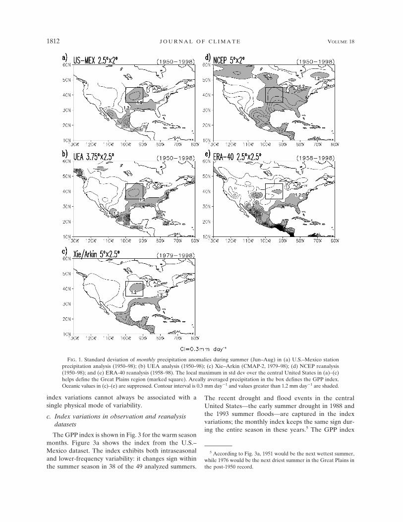
The extent of interannual variability in warm seasonprecipitation is examined in Fig. 1 by displaying thestandard deviation (SD) of monthly precipitationanomalies in observations (Figs. 1a–c) and reanalysisdatasets (Figs. 1d,e) over North America. The two sta-tion datasets are similar over the United States, with alocal maximum in interannual precipitation variabilityover the Great Plains region. The UEA data exhibitmarginally greater variability in the coastal regions, de-spite its coarseness; grid-averaged precipitation can,however, be influenced by orographic resolution in anunpredictable manner in coastal zones. The satellite-based Xie–Arkin precipitation has an interannual vari-ability range that is similar to the surface-based records;the amplitude is a bit weaker, though, especially overthe Great Plains where the maximum is now less than1.5 mm day�1. Comparison of the three standard de-viations in the same 20-yr subperiod (1979–98) showsthat weaker variability in Fig. 1c is not an artifact of theperiod differences; the discrepancy over Great Plains is,

if anything, greater now, with the U.S.–Mexico data ex-hibiting an amplitude in excess of 1.8 mm day�1 in places.

The depiction of warm season precipitation variabil-ity in the reanalysis datasets (Figs. 1d,e) is quasi real-istic. Although the southeastern focus is captured inboth, ERA-40 underestimates while NCEP overesti-mates the magnitude of interannual variability in theOhio Valley and Great Plains regions; NCEP’s ten-dency to overestimate precipitation variability has beennoted before (e.g., Janowiak et al. 1998). The higherresolution of ERA-40 is evident from the presence ofsmall-scale features in Fig. 1e and from the very largeamplitudes over portions of Mexico and CentralAmerica; also evident is a spurious feature over Colo-rado and New Mexico.

Warm season precipitation variability in the AMIPsimulations is shown in Fig. 2. The simulations are inreasonable agreement among themselves and with ob-servations over the western United States, but somedifferences are evident in the eastern half. The localmaximum over the Great Plains is somewhat diffusebut otherwise well positioned in the CAM simulation.The same feature in the NSIPP simulation is too strong(�2.1 mm day�1) and westward shifted in comparisonwith observations. The Gulf Coast focus is also missingin the CAM simulation. It is noteworthy that the inter-annual variability of Great Plains precipitation is large,being 30%–50% of the climatology in most places.

b. Index definition

An index is often used to describe the temporal vari-ability of a spatially coherent region. One such region ismarked in the Fig. 1 panels. The square box (35°–45°N,100°–90°W) evidently encompasses the region exhibit-ing a local maximum in observed precipitation variabil-ity (Figs. 1a–c). The boxed region includes the states ofSouth Dakota, Minnesota, Wisconsin, Nebraska, Iowa,Illinois, Kansas, Missouri, Oklahoma, and Arkansas,and extends from the northeast corner of the Tier-2sector into the Tier-3 sector of the NAME domain(Amador et al. 2004).

The areal average of precipitation in the box definesthe Great Plains Precipitation (GPP) index. A similarindex was used by Ting and Wang (1997) and Mo et al.(1997) to track precipitation variability in the centralUnited States; Schubert et al. (2004) have, however,used a more meridionally extended box for index defi-nition.4 Although indices remain attractive in charac-terizing variability because of their intrinsic simplicity,

4 Other index definitions: Ting and Wang’s: 32.5°–45°N, 105°–85°W; Mo et al.’s: 34°–46°N, 105°–85°W; and Schubert et al.’s:30°–50°N, 105°–95°W.


index variations cannot always be associated with asingle physical mode of variability.

c. Index variations in observation and reanalysisdatasets

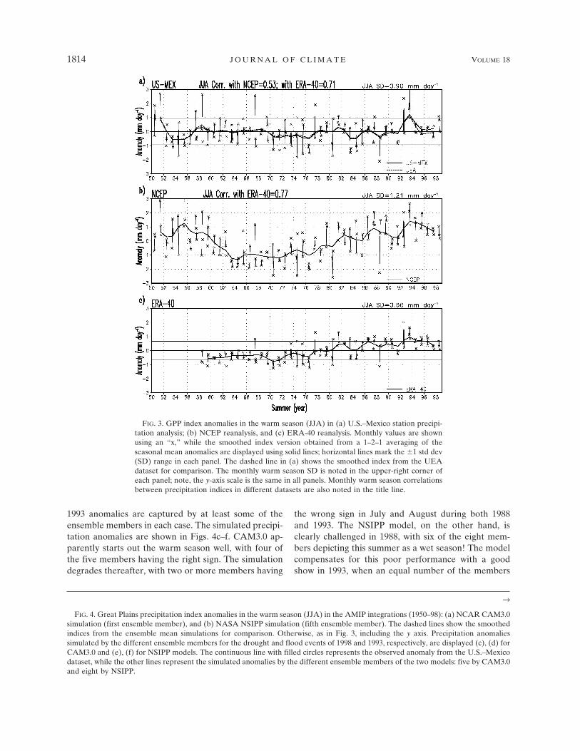
The GPP index is shown in Fig. 3 for the warm seasonmonths. Figure 3a shows the index from the U.S.–Mexico dataset. The index exhibits both intraseasonaland lower-frequency variability: it changes sign withinthe summer season in 38 of the 49 analyzed summers.

The recent drought and flood events in the centralUnited States—the early summer drought in 1988 andthe 1993 summer floods—are captured in the indexvariations; the monthly index keeps the same sign dur-ing the entire season in these years.5 The GPP index

5 According to Fig. 3a, 1951 would be the next wettest summer,while 1976 would be the next driest summer in the Great Plains inthe post-1950 record.

FIG. 1. Standard deviation of monthly precipitation anomalies during summer (Jun–Aug) in (a) U.S.–Mexico stationprecipitation analysis (1950–98); (b) UEA analysis (1950–98); (c) Xie–Arkin (CMAP-2, 1979–98); (d) NCEP reanalysis(1950–98); and (e) ERA-40 reanalysis (1958–98). The local maximum in std dev over the central United States in (a)–(c)helps define the Great Plains region (marked square). Areally averaged precipitation in the box defines the GPP index.Oceanic values in (c)–(e) are suppressed. Contour interval is 0.3 mm day�1 and values greater than 1.2 mm day�1 are shaded.


calculated using NCEP and ERA-40 reanalysis isshown in Figs. 3b,c using the same scale. Index varia-tions are robust in the NCEP reanalysis; the JJAmonthly SD being 1.21 mm day�1, in comparison with0.90 mm day�1 in the U.S.–Mexico dataset (Fig. 3a).The ERA-40 index, on the other hand, exhibits weakervariations, with a SD of only 0.66 mm day�1. The tworeanalysis indices are however closer together in track-ing the anomalies (correlated at 0.77); NCEP is corre-lated with observations at 0.53, while ERA-40 is morestrongly correlated at 0.71, all at monthly resolution.

Interannual variability is highlighted in Fig. 3 bysolid, continuous lines, produced from the 1–2–1smoothing of the summer-mean index anomalies.6 Fig-ure 3a shows the smoothed indices from U.S.–Mexico(solid) and UEA (dashed) datasets, and their substan-

tial overlap attests to their closeness in the Great Plainsregion; the monthly summer correlation is 0.98. In con-trast with observations, the smoothed reanalysis indicesshow an upward trend in Great Plains precipitationsince the mid-1960s. Discrepancy with observations isespecially pronounced in the earlier part of the record(1950–70) and leads to reduced correlations: 0.33 forNCEP and 0.55 for ERA-40, as opposed to the in-creased NCEP-ERA-40 correlation of 0.88. An inter-esting discrepancy in the latter part is the marginal rep-resentation of the 1988 early summer drought in thereanalysis datasets, particularly, NCEP.

d. Index variations in AMIP simulations

The GPP index from the AMIP simulations is shownin Fig. 4. The CAM simulation (Fig. 4a) exhibits a re-alistic range of variability; the JJA monthly standarddeviation is 0.96 mm day�1, that is, very close to theobserved value. The NSIPP simulation is equally goodin this respect with a 0.99 mm day�1 amplitude. Thetemporal structure of variability however leaves muchto be desired in both simulations. CAM is correlatedwith the observed index at 0.11, while NSIPP is corre-lated at �0.09, all at monthly resolution; the eight-member7 unsmoothed NSIPP ensemble mean (notshown) is also poorly correlated (0.04), as is the corre-sponding five-member CAM3.0 ensemble mean (0.15).That the 1988 and 1993 summers are not notablyanomalous over the Great Plains in the model simula-tions is testimony to the poor temporal correlations.Precipitation is, in fact, excessive in the NSIPP simula-tion in the 1988 summer! The CAM and NSIPP simu-lations are thus unable to produce realistic monthly pre-cipitation variability over the Great Plains, and the cor-responding ensemble means fare no better.

But could seasonal (and lower frequency) variabilitybe somewhat more realistically represented in thesesimulations? The question is pertinent since the modelsare, presently, unable to generate realistic intraseasonalvariability. Smoothed versions of the indices are dis-played in Figs. 4a,b to highlight the longer time scales;smoothed versions of the ensemble mean indices arealso shown using a dashed line. A visual comparison ofthe smoothed indices with their observational counter-part (Fig. 3a) shows little traction, and this is reflectedin the limited correlations: 0.25 for CAM and 0.06 forNSIPP. The ensemble means do somewhat better with0.59 for CAM and 0.30 for NSIPP.

That still leaves open the possibility that the 1988 and

6 The smoothed index is thus based on the preceding, current,and subsequent summer means.

7 Data archiving problems during model integration precludedthe use of one ensemble member.

FIG. 2. Standard deviation of monthly precipitation anomaliesduring summer (Jun–Aug) in the AMIP integrations (1950–98):(a) NCAR CAM3.0 simulation (first ensemble member), and (b)the NSIPP simulation (fifth ensemble member). The marked boxoutlines the Great Plains region defined earlier using observedprecipitation variability. Oceanic values are suppressed; contour-ing as in Fig. 1.


1993 anomalies are captured by at least some of theensemble members in each case. The simulated precipi-tation anomalies are shown in Figs. 4c–f. CAM3.0 ap-parently starts out the warm season well, with four ofthe five members having the right sign. The simulationdegrades thereafter, with two or more members having

the wrong sign in July and August during both 1988and 1993. The NSIPP model, on the other hand, isclearly challenged in 1988, with six of the eight mem-bers depicting this summer as a wet season! The modelcompensates for this poor performance with a goodshow in 1993, when an equal number of the members

→

FIG. 4. Great Plains precipitation index anomalies in the warm season (JJA) in the AMIP integrations (1950–98): (a) NCAR CAM3.0simulation (first ensemble member), and (b) NASA NSIPP simulation (fifth ensemble member). The dashed lines show the smoothedindices from the ensemble mean simulations for comparison. Otherwise, as in Fig. 3, including the y axis. Precipitation anomaliessimulated by the different ensemble members for the drought and flood events of 1998 and 1993, respectively, are displayed (c), (d) forCAM3.0 and (e), (f) for NSIPP models. The continuous line with filled circles represents the observed anomaly from the U.S.–Mexicodataset, while the other lines represent the simulated anomalies by the different ensemble members of the two models: five by CAM3.0and eight by NSIPP.

FIG. 3. GPP index anomalies in the warm season (JJA) in (a) U.S.–Mexico station precipi-tation analysis; (b) NCEP reanalysis, and (c) ERA-40 reanalysis. Monthly values are shownusing an “x,” while the smoothed index version obtained from a 1–2–1 averaging of theseasonal mean anomalies are displayed using solid lines; horizontal lines mark the �1 std dev(SD) range in each panel. The dashed line in (a) shows the smoothed index from the UEAdataset for comparison. The monthly warm season SD is noted in the upper-right corner ofeach panel; note, the y-axis scale is the same in all panels. Monthly warm season correlationsbetween precipitation indices in different datasets are also noted in the title line.



get the sign (if not the amplitude) of the precipitationanomaly right. Overall, CAM3.0 appears to be morediscriminating, though.

Modest values of the ensemble mean correlationsshould not however be taken to be reflective of theextent of SST influence on Great Plains precipitation innature since model deficiencies could easily interferewith the realization of the potential influence. Obser-vational analyses indicate the SST linkage to be some-what (but not considerably) stronger. Schubert et al.(2004) report stronger links between Great Plains pre-cipitation and Pacific SSTs in more extended NSIPPsimulations, albeit at lower frequencies (time scalesgreater than 6 yr). Models are clearly in need of furtherrefinements, especially in the representation of interac-tions between dynamical and thermodynamical pro-cesses.

e. Index variations from convective and stratiformrainfall

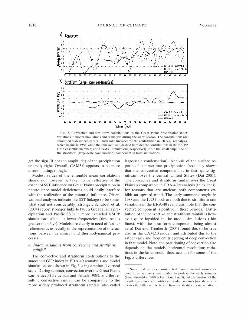
The convective and stratiform contributions to thesmoothed GPP index in ERA-40 reanalysis and modelsimulations are shown in Fig. 5 using a reduced verticalscale. During summer, convection over the Great Plainscan be deep (Heideman and Fritsch 1988), and the re-sulting convective rainfall can be comparable to themore widely produced stratiform rainfall (also called

large-scale condensation). Analysis of the surface re-ports of summertime precipitation frequency showsthat the convective component is, in fact, quite sig-nificant over the central United States (Dai 2001).The convective and stratiform rainfall over the GreatPlains is comparable in ERA-40 reanalysis (thick lines);for reasons that are unclear, both components ex-hibit an upward trend. The early summer drought in1988 and the 1993 floods are both due to stratiform rainvariations in the ERA-40 reanalysis: note that the con-vective component is positive in these periods.8 Distri-bution of the convective and stratiform rainfall is how-ever quite lopsided in the model simulations (thinlines), with the stratiform component being almostzero! Dai and Trenberth (2004) found this to be truealso in the CAM2.0 model, and attributed this to therather early and frequent triggering of deep convectionin that model. Note, the partitioning of convection alsodepends on the models’ horizontal resolution; varia-tions in the latter could, thus, account for some of theFig. 5 differences.

8 Smoothed indices, constructed from seasonal anomaliesover three summers, are unable to portray the early summer(June) drought in 1988 in Fig. 5 (and Fig. 3), but examination of themonthly, unsmoothed partitioned rainfall amounts (not shown) in-dicates the 1988 event to be also linked to stratiform rain variations.

FIG. 5. Convective and stratiform contributions to the Great Plains precipitation indexvariations in model simulations and reanalysis during the warm season. The contributions aresmoothed as described earlier. Thick solid lines denote the contribution in ERA-40 reanalysis,which begins in 1958, while the thin solid and dashed lines denote contributions in the NSIPP(fifth ensemble member) and CAM3.0 simulations, respectively. Note the small amplitude ofthe stratiform (large-scale condensation) component in both simulations.


4. Great Plains precipitation linkages

a. Precipitation structure

The GPP index is regressed on the U.S.–Mexico datain Fig. 6a; the index is derived from the same data, aswell. Regressions are strongest over the Great Plains, asexpected, but Great Plains precipitation is apparentlynot linked with significant precipitation anomalies else-where on the continent—quite unlike the case duringseasonal onset of the North American monsoon, whena compensatory structure is present across the southerntier states in July (e.g., Barlow et al. 1998). The GPPindex regressions on NCEP and ERA-40 reanalysisprecipitation are shown in Figs. 6b,c, respectively; theindices are derived from the respective precipitationdatasets. The reanalysis distributions are not as region-ally confined as in Fig. 6a, but exhibit subcontinentalscales, particularly NCEP’s, which shows the GreatPlains precipitation anomaly to be part of a much largerwet pattern covering the central and eastern UnitedStates. The ERA-40 regressions are somewhat weakerover the Great Plains (�1.2 mm day�1), in line withexpectations (cf. Figs. 1 and 3).

b. Reanalysis moisture fluxes

Moisture fluxes associated with the Great Plains pre-cipitation anomalies are shown in Figs. 6d–g. The fluxesare obtained from 6-hourly reanalysis data, and the sta-tionary and transient components are shown separatelyafter vertical integration over the surface to 300-hPalayer, that is,

�300hPa

Psur

qV dp�g; �300hPa

Psur

q�V� dp�g,

respectively. Here q is the specific humidity, V the hori-zontal wind vector; the overbar denotes the monthlymean, and the prime the deviation from it. More pre-cisely, stationary and transient fluxes were calculated at00000, 0600, 1200, and 1800 UTC of each month andthen averaged in order to preclude aliasing of the diur-nal cycle. The NCEP surface pressure field was used inboth diagnoses since this field was not readily (orfreely) available in ERA-40 reanalysis; in retrospect,this choice was good for comparisons. Data from theadditional lower-tropospheric level in ERA-40 reanaly-sis (775 hPa) was not used in computation of the ver-tical integral so that the two moisture fluxes can beclosely compared.9

The stationary moisture fluxes linked with GreatPlains precipitation variability in NCEP and ERA-40

reanalysis are broadly similar over North America (cf.Figs. 6d,e). In both cases, fluxes are onshore over theGulf coast and then northeastward oriented; however,fluxes and flux convergences are stronger in ERA-40 bya factor of up to 2. Interesting differences are also evi-dent over the American Tropics, especially, the Carri-bean Sea, where ERA-40 has robust westward fluxes.The fluxes are part of a coherent, large-scale, low-level10

anticyclonic circulation that connects with the southerlyfluxes over the U.S. Gulf Coast, much as in the westernflank of the Bermuda high (a prominent feature of thesummertime sea level pressure field over the Atlantic).It is noteworthy that flux convergence accounts formuch of the Great Plains precipitation in ERA-40.

The transient moisture fluxes linked with GreatPlains precipitation variability (Figs. 6f,g) are substan-tially smaller than the stationary ones. The vector scalein these panels is smaller by a factor of 5; the fluxconvergence is, however, smaller by only a factor of2–3. The transient fluxes are westward over the easternUnited States in both reanalyses, but the ERA-40 onesare stronger and more convergent, particularly, over

9 Separate analysis of the influence of 775-hPa data on verticallyintegrated moisture fluxes shows the impact to be modest.

10 Moisture weighting in the vertical integral highlights thelower-tropospheric circulation features.

FIG. 6. Warm season regressions of the Great Plains precipita-tion index on (a) U.S.–Mexico station precipitation, (b) NCEPprecipitation, (c) ERA-40 precipitation, (d) NCEP stationarymoisture fluxes, (e) ERA-40 stationary moisture fluxes, (f) NCEPtransient moisture fluxes, and (g) ERA-40 transient moisturefluxes. Note that the index and regressions are from the samemonthly dataset in each case. Moisture fluxes in (d)–(g) are ver-tically integrated (300 hPa to the surface), and the flux conver-gence is also shown. Both precipitation and moisture flux conver-gence are contoured with the same interval (0.3 mm day�1); dark(light) shading denotes areas of positive (negative) rainfall andmoisture flux convergence (divergence) in excess of 0.3 mm day�1

magnitude; the zero contour is omitted. The vector scale for fluxesis shown at the bottom of each panel; note the 5-times larger scalein the display of the stationary component.


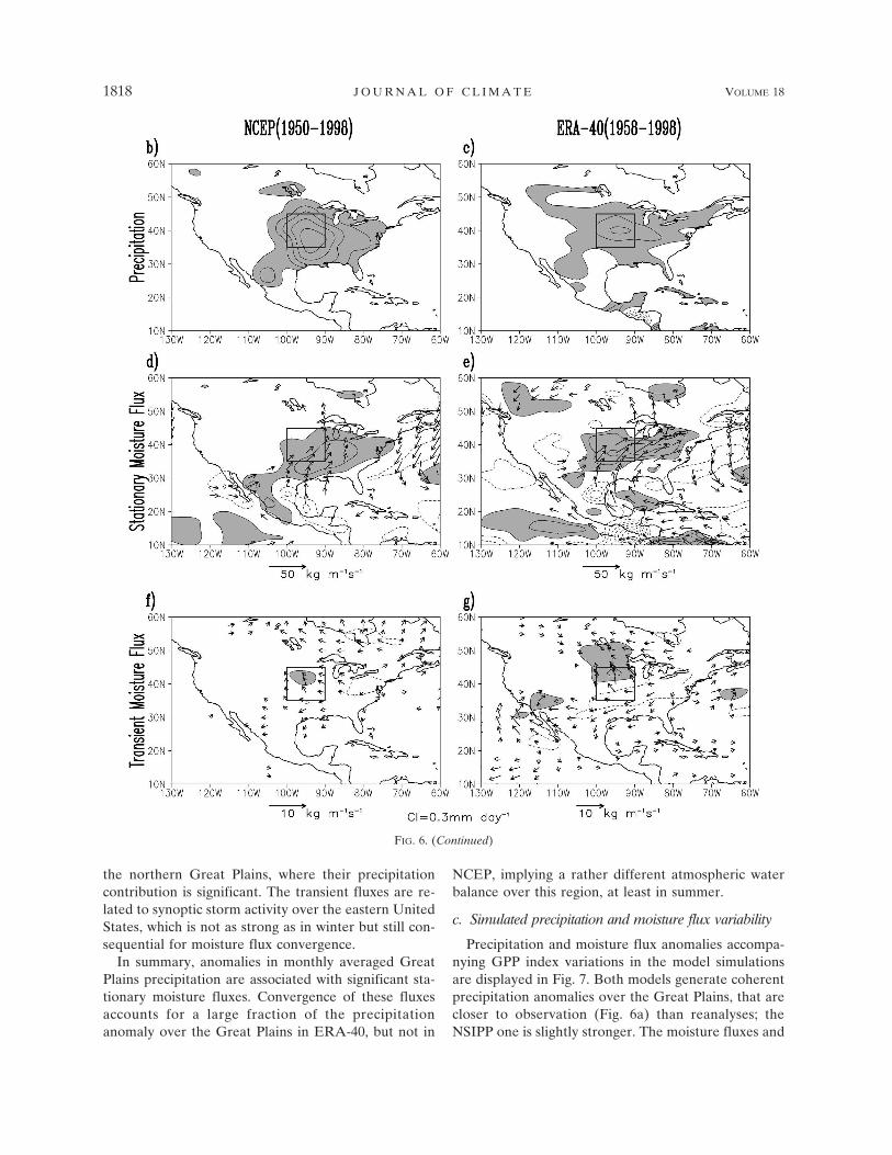
the northern Great Plains, where their precipitationcontribution is significant. The transient fluxes are re-lated to synoptic storm activity over the eastern UnitedStates, which is not as strong as in winter but still con-sequential for moisture flux convergence.

In summary, anomalies in monthly averaged GreatPlains precipitation are associated with significant sta-tionary moisture fluxes. Convergence of these fluxesaccounts for a large fraction of the precipitationanomaly over the Great Plains in ERA-40, but not in

NCEP, implying a rather different atmospheric waterbalance over this region, at least in summer.

c. Simulated precipitation and moisture flux variability

Precipitation and moisture flux anomalies accompa-nying GPP index variations in the model simulationsare displayed in Fig. 7. Both models generate coherentprecipitation anomalies over the Great Plains, that arecloser to observation (Fig. 6a) than reanalyses; theNSIPP one is slightly stronger. The moisture fluxes and

FIG. 6. (Continued)


their convergence are shown in Figs. 7c–e. The focus ison the stationary component since it is dominant andalso because the transient component could not be cal-culated for the CAM simulation as this field was un-available in the online data archives at NCAR. Themoisture fluxes are quite different in the two simula-tions. The CAM fluxes suggest that GPP variations are

accompanied by a low-level circulation over the south-eastern United States, with a limited transport over theGulf of Mexico in contrast with the coherent anticy-clonic structure with an extended fetch that is present inthe NSIPP simulation (and ERA-40 reanalysis). Notsurprisingly, CAM is unable to generate sufficientmoisture flux convergence over the Great Plains. The

FIG. 7. Warm season regressions of the Great Plains precipitation index in AMIP simulations (1950–98): (a) CAM3.0precipitation, (b) NSIPP precipitation, (c) CAM3.0 stationary moisture fluxes, (d) NSIPP stationary moisture fluxes, and(e) NSIPP transient moisture fluxes. Note that the index and regressions come from the same monthly dataset in eachcase. All NSIPP regressions are from the fifth ensemble member while the CAM ones are from the first ensemblemember. Transient fluxes are not shown for CAM3.0 since the zonal component was not archived; otherwise, as in Fig. 6.


NSIPP simulation, on the other hand, has quasi-realisticmoisture fluxes, especially, in comparison with theERA-40 fluxes.

d. Diagnosed and simulated evaporation

The relative contribution of local and remote watersources in generation of Great Plains precipitation vari-ability motivates the examination of the evaporationfield. Evaporation observations are, unfortunately,rather limited and seldom representative of the larger-scale hydroclimate conditions. Good long-term mea-surements are generally available only in sublatitude–longitude degree basins [e.g., the United States Depart-ment of Agriculture (USDA) monitored watersheds,Oklahoma Mesonet] and, as such, the large-scaleevaporation field must often be diagnosed from reason-ably validated land surface models driven by circula-tion, temperature, and precipitation observations. Note,the reanalysis evaporation is constrained only by circula-tion and temperature observations, that is, less directly.

Two evaporation diagnoses are analyzed here: Thefirst is produced at NOAA CPC from a one-layer hy-drological model (Huang et al. 1996; more informationavailable online at http://www.cpc.ncep.noaa.gov/soilmst/index.htm). The model is driven by observedsurface air temperature and precipitation and yieldsevaporation and runoff estimates for the 344 climatedivisions: the model is tuned with observed runoff datain Oklahoma and estimates are available for the 1931–present period. The second diagnosis was conducted atCOLA using their Simplified Simple Biosphere model(SSiB) (Xue et al. 1991). The diagnosis was undertakenfor the 1979–99 period and is referred as the GlobalOffline Land surface Data-set (GOLD, more informa-tion available online at http://www.iges.org/gold; Dirm-eyer and Tan 2001).11

The GPP index regressions on diagnosed evapora-tion are shown in Figs. 8a,b. The GOLD estimates arealmost a factor of 3 larger than the CPC ones, and thisdiscrepancy cannot be attributed to the record-lengthdifferences. Interestingly, both estimates depict a maxi-mum in the southwest corner of the boxed region (i.e.,Oklahoma), which supplies the runoff observations formodel tuning, at least in CPC’s diagnosis. The corre-sponding regressions on the NCEP and ERA-40 re-analysis evaporation fields are shown in Figs. 8c,d, re-spectively: note that reanalysis evaporation is not con-

strained by precipitation and runoff observations. Thereanalysis evaporation anomalies over the Great Plainsare, apparently, as far apart as the two diagnosedanomalies; the NCEP anomaly ranges from 0.1 to 0.3mm day�1—not unlike the GOLD estimates—whilethe ERA-40 anomaly is not even up to the contouringthreshold (0.1 mm day�1), much like the CPC-basedestimate.

The evaporation anomalies accompanying GreatPlains precipitation variations in the model simulationsare shown in Figs. 8e,f. They are phenomenally strong,reaching 1.0–1.2 mm day�1; in both cases, the anoma-lies are focused over the Great Plains. The very largevalues of local evaporation in the models—up to 4times larger than the highest observationally con-strained estimate (i.e., NCEP’s)—suggest a significantlydifferent view of the anomalous atmospheric water bal-ance, one in which local water sources (precipitationrecycling) contribute overwhelmingly to Great Plainsprecipitation variability. For example, evaporation con-tributes nearly twice as much as the stationary moisturefluxes to Great Plains precipitation variability in bothCAM and NSIPP simulations. The case is quite theopposite in the reanalyses, with the stationary moistureflux contributions being dominant; the flux conver-gence is about 1.5 times larger than evaporation inNCEP and even larger in ERA-40 data. [The finding ofthe dominance of evaporation over moisture flux con-vergence in the NSIPP model explains why Koster et al.(2003) find land—atmosphere feedback to be so impor-tant in accounting for the July precipitation variance inNSIPP simulations of Great Plains hydroclimate vari-ability.]

Intercomparison of both evaporation anomaliesand their relative contribution in generating GreatPlains precipitation variability suggests that theseanomalies are, perhaps, too strong in the modelsimulations—possibly outliers in comparison with thereanalysis and diagnosed evaporation estimates. Al-though this assessment will need to be corrobo-rated from multimodel estimates of evaporation thatwill be produced by the Global Soil Wetness Proj-ect (GSWP-2, version 2; Dirmeyer et al. 2002; moreinformation available online at http://grads.iges.org/gswp2/), it appears that land surface–atmosphere in-teractions are overemphasized in the models, at leastin context of the warm season hydroclimate variabilityover North America—a distinct possibility if the modelland surface schemes were tuned using climatologicalreanalyses data alone. The model evaporation clima-tologies over the United States (especially NSIPP’s) arecomparable to the reanalysis counterparts, but are

11 The precipitation used in generating the GOLD dataset ishighly correlated with the U.S.–Mexico precipitation data; theGPP indices are correlated at 0.96.


much too strong vis-a-vis the diagnosed GOLD andCPC evaporation climatologies—by up to a factor of 2.

e. Observed and simulated SST links

The SST links to Great Plains precipitation variabil-ity are identified from correlations of the smoothed

GPP indices (shown in Figs. 3–4) and displayed in Fig.9. The smoothed index versions are used in order tohighlight linkages on the seasonal to interannual timescales, while correlations are computed instead of re-gressions in order to assess the significance of SST link-ages in the context of interannual variability. Correla-

FIG. 8. Warm season regressions of the Great Plains precipitation index on evaporation (surface latent heat flux): (a)evaporation diagnosed from NOAA/CPC one-layer hydrologic model (see text for details), (b) another diagnosis ofevaporation (GOLD dataset; see text for details), (c) NCEP evaporation, (d) ERA-40 evaporation, (e) CAM3.0 evapo-ration (first ensemble member), and (f) NSIPP evaporation (fifth ensemble member). Note that the regression periodstated in the title line varies somewhat. Regressions in (a) are against the GPP index constructed from the U.S.–Mexicodataset; in the remaining panels, the index and regressions are from the same dataset. The contour interval and shadingthreshold is 0.1 mm day�1, with positive values shaded dark; the zero contour is omitted in all panels.


tions of the precipitation index derived from the U.S.–Mexico station data are shown first in Fig. 9a, as theyare the simulation target. SST correlations exhibit acoherent, basin-scale structure that resembles the Pa-cific decadal variability pattern in many respects. Thelargest correlations (�0.5) are in the Gulf of Alaska,

the midlatitude Pacific (date line sector),12 and in anortheastward-oriented band emanating from the

12 This region exhibits the strongest correlation (�0.5) with theunsmoothed version of the seasonal GPP index.

FIG. 9. Warm season SST correlations of the smoothed Great Plains precipitation index(1950–98). The smoothed index is from (a) the U.S.–Mexico station precipitation analysis, (b)CAM3.0 simulation (first ensemble member), (c) CAM3.0’s five-member ensemble meansimulation, and from (d) NSIPP’s eight-member ensemble mean simulation. Correlations havebeen smoothed using adjacent grid points (smth9 in GrADS). Contour interval is 0.1 and dark(light) shading denotes positive (negative) correlations in excess of 0.4 magnitude. The zerocontour is omitted in all panels.


equatorial central Pacific. The correlation structurerules out contemporaneous linkage between ENSO andthe smoothed, seasonally averaged Great Plains pre-cipitation.13 The finding on connections with the extra-tropical Pacific SSTs is not a new one; Ting and Wang(1997), Higgins et al. (1999), Nigam et al. (1999), Lauand Weng (2000), and Barlow et al. (2001) have allinvestigated aspects of this linkage.

SST correlations of CAM’s smoothed GPP indicesare shown in Figs. 9b,c. Correlations of the first en-semble member’s index exhibit coherent structure inthe tropical Pacific, similar to the target structure (Fig.9a). Correlations of the ensemble mean index are evencloser to Fig. 9a; note the striking similarity in the mid-latitude basins. The correlations are however somewhatstronger in the central equatorial Pacific (�0.6), point-ing to this region’s greater connectivity with the GreatPlains in CAM3.0. The corresponding correlations ofNSIPP’s ensemble mean index (Fig. 9d) are qualita-tively similar, but are not as close to the target structureas CAM’s; especially in the western midlatitude basins.Longer AMIP simulations with the NSIPP model(Schubert et al. 2004) indicate stronger links with Pa-cific SSTs in the entire tropical basin (correlations�0.6–0.7 using an all-year index); reasons for the dis-crepancy are unclear, but the use of highly smoothedSSTs and GPP index (retaining 6-yr or longer timescales) likely contributes to the higher correlation.

The extent to which Figs. 9b,c differ is surprising be-cause the internally generated (random) variabilityshould have been filtered out during computation ofthe correlation. As discussed earlier (cf. footnote 3), anensemble of AMIP-type climate simulations can help inapportioning a particular summer’s anomaly into its in-ternal and SST-forced variability components. But asimulation ensemble would be deemed to have consid-erable redundancy in the context of extraction of thecharacteristic (dominant) patterns of interannual vari-ability, especially, if each simulation was of sufficientduration [e.g., the case here (�50 yr)]. Correlationanalysis on a single ensemble member of such lengthshould have sufficed in filtering the internally gener-ated (random) component of variability.

f. Antecedent SST links in observations

The SST links shown above are all contemporaneousand, hence, not revealing of the direction of influence.Causality is investigated by computing correlations ofthe July GPP index (derived from the U.S.–Mexico sta-tion data) with antecedent SSTs. July’s index is chosenas a reference since the standard deviation of monthlyprecipitation is strongest in this month and, also, be-cause July is in the middle of the warm season. TheSST-leading correlations are shown in Fig. 10 atmonthly resolution starting in April; the correlationsare computed with the unsmoothed version of the in-dex. The antecedent correlations are seldom largerthan 0.4 but exhibit a coherent structure similar to thatseen earlier (Fig. 9a).

The antecedent SST structure over the Pacific (Figs.10a–c) is broadly similar to the contemporaneous SSTlinks (Fig. 10d), especially at basin scales except forregional developments in the extratropical basin (atmo-sphere forced?). A meridional expansion of the equa-torial Pacific feature with time is also evident. Theshape evolution is intriguing, with the focal point mov-ing to the northern off-equatorial latitudes in summer.But, are the 0.3–0.4 correlations significant, especiallyagainst the backdrop of decadal variability in the Pa-cific and Atlantic basins? A careful examination of thisissue is beyond the scope of this paper, but a rudimen-tary analysis involving SST correlations with a random-ized version of the GPP index yields contemporaneouscorrelations in the �0.2 range in July, that is, marginallyweaker than those in Fig. 10d. The obtained correlationstructure (not shown) is however quite different (inco-herent) from that in Fig. 10d, particularly in the easternPacific.

Correlations with the randomized index are howevernot devoid of coherency in the Atlantic basin. For thisreason, the interesting evolution of Atlantic SSTs inFig. 10 is noted, but not further discussed. Three zon-ally oriented bands characterize the precursor-periodstructure, especially, in May–June. The banded SSTsare, in fact, reminiscent of the interhemispheric vari-ability mode (cf. Fig. 10 in Ruiz-Barradas et al. 2000),which is also energetic in spring.14 Interestingly, thebands in the extratropical Atlantic flip sign in July butthe significance of this, if any, is unclear. Additionallag–lead analysis and modeling experiments are clearlyneeded to understand the SST linkages and their sig-nificance for U.S. hydroclimate variability.

13 This is consistent with Barlow et al.’s (2001) analysis, whichshows a monthly evolution in ENSO’s impact on U.S. precipita-tion (cf. Fig. 5); the impact is, in fact, opposite at the beginning(June) and end (August) of the warm season, particularly alongthe East Coast and in the Great Plains. Absence of the ENSOsignature in SST links of the seasonally averaged GPP index isthus not surprising; the 1–2–1 smoothing of the GPP index acrossthree summer seasons must further diminish the linkage.

14 The mode has also been referred to as the Pan–Atlantic dec-adal oscillation pattern (Xie and Tanimoto 1998).


5. Recurrent patterns of warm season SST andgeopotential (�700) variability

The analysis moves away from its continental-centricprecipitation focus in this section. The Great Plains pre-cipitation index is no longer the fulcrum, but the target

here. The motivation stems from generic concerns as-sociated with physical indices, namely, that index varia-tions can reflect the superposed effects of two or moreindependent modes of variability, thereby confoundingunderstanding of the variability mechanisms. There isalready some indication of the GPP index’s linkage

FIG. 10. SST-leading correlations with the Jul Great Plains precipitation index (1950–98).The index is derived from the U.S.–Mexico station precipitation dataset, and correlations arecomputed with the unsmoothed version of the index: (a) Apr SST correlations, (b) May SSTcorrelations, (c) Jun SST correlations, and (d) Jul SST correlations (contemporaneous). Cor-relations have been smoothed using adjacent grid points (smth9 in GrADS). Contour intervalis 0.1 and dark (light) shading denotes positive (negative) correlations in excess of 0.4 mag-nitude. The zero contour is omitted in all panels.


with the Pacific and Atlantic basins that display ratherdifferent spatiotemporal variability. Unraveling the con-tribution of the different variability modes in GPP indexvariations should advance the understanding, modeling,and prediction of Great Plains hydroclimate variability.

The SST and lower-tropospheric geopotential (�700)variability during boreal summer months (JJA) is ob-jectively analyzed here. Geopotential height compactlyrepresents the winds in the extratropical domain (theregion of interest), and its variability at the 700-hPalevel is analyzed in order to focus on the circulationcomponent that is important for moisture transports.15

Having a variable each from the ocean and atmosphereprecludes the analysis from being SST centric (as inBarlow et al. 2001) or Great Plains centric (as in thepreceding sections).

The analysis strategy is influenced by Lanzante’s(1984) study, published two decades ago. The study isnotable for several reasons: it provided the first objec-tive analysis of interannual circulation variability in thewarm season months; it assessed the circulation’s link-age with Pacific and Atlantic SSTs within the frame-work of a single analysis; it corroborated important as-pects of Namias’s (1983; and earlier papers) analysis ofantecedent/coincident drought circulations and SSTs, inparticular, by showing the presence of a Pacific–NorthAmerican (PNA)-like circulation pattern in the springand summer months (i.e., well outside of the winter sea-son); and it extended the correlation analysis technique(Prohaska 1976) through the use of varimax rotation.

The present analysis is motivated by the need to cor-roborate Lanzante’s (1984) findings using a longer ob-servational record—one that includes data from bothbefore and after the 1976–77 climate transition (e.g.,Trenberth 1990). Lanzante analyzed the 1949–78 pe-riod (i.e., essentially, the pretransition period). Rotatedprincipal component analysis (RPCA) is used to iden-tify the recurrent patterns here, as opposed to rotatedcanonical correlation analysis in Lanzante. The RPCAmethod analyzes the structure of cross-correlation andautocorrelation matrices whereas the canonical corre-lation technique focuses only on the former. Despitethis difference, the two methods yield similar results, asascertained from the RPCA of the 1949–78 record. Theleading structures are similar to those shown in Lan-zante; minor pattern differences can be as easily attrib-uted to SST and geopotential data differences as to theanalysis method differences.

The combined variability of SST (Hadley) and 700-hPa geopotential (NCEP reanalysis) in the extratropi-cal Pacific and Atlantic sectors (25°–75°N, 155°E–15°W) during the 1950–98 warm season months ofJune–August is analyzed. The variables are scaled by(cos �)1/2 to achieve grid-area parity on a regular lati-tude–longitude grid, and put on par with each other bynormalizing their anomalies by the square root of theirspatially integrated temporal variance; the advantagesof such a normalization are discussed in Nigam andShen (1993). Nine loading vectors are rotated and theresulting two that are related to Great Plains hydrocli-mate variability are discussed in this section. Thesemodes are robust in that they are also obtained fromrotation of the six leading loading vectors.16

a. The Pacific connection

The rotated principal component (PC) most stronglycorrelated with the GPP index in the warm seasonmonths is shown in Fig. 11d. The correlation is �0.43; itis the seventh leading mode in a ranking based on ac-counting of the SST and �700 variance in the analysisdomain. The SST anomalies are prominent in the Gulfof Alaska and in the central and eastern equatorial Pa-cific; the causative influence of the latter is being inves-tigated. The covariant �700 anomalies are confined tothe PNA sector with a structure that is somewhat remi-niscent of the wintertime PNA pattern (e.g., Wallaceand Gutzler 1981; Nigam 2003). The negative SSTanomalies in the Gulf of Alaska likely arise from en-hanced westerlies and, consequently, enhanced surfacefluxes and Ekman pumping in that sector, assumingthat 700-hPa anomalies are representative of the near-surface circulation as well, a likely scenario. The SSTand geopotential anomalies resemble a leading summerpattern in Lanzante’s analysis (1984; Fig. 2c) except forthe missing trough over the southern states in Fig. 11a.The PNA-like, warm season height anomalies are re-ferred to as the “Great Plains” pattern in Lanzantesince they are structurally similar (but oppositelysigned) to the composited anomalies for the 1952–54drought summers (Fig. 4 of Namias 1983).

The PC exhibits both intraseasonal (defined by a signchange within a season) and lower-frequency variabil-ity; the sign changes in 27 of the 49 summer seasons.The PC is positive during the 1988 summer (a recentshort drought) and in other summers as well (e.g., 1970,1973, 1984), some of which were drier than normal (cf.

15 The 850-hPa level was not chosen because of its being belowthe surface over large areas of North America, and because it wasdeemed to be somewhat disconnected from the upper-level flow(i.e., the medium connecting remote regions).

16 Analysis of an extended warm season, with an additionalmonth at the beginning (May) or the end (September), yields thesame modes, as does the analysis in a larger domain (20°S–75°N,0°–360°).


Fig. 3a). Given the role of the 1952–54 drought in thenaming of this anomaly pattern, it would be of someinterest to examine the drought’s representation in Fig.11d; unfortunately, the drought is not captured sincenegative PC values indicate wetness (Fig. 11b). Accord-ing to the PC, the 1950–53 summers is a wet period,whereas in nature (Fig. 3a) the drought onset occurredin 1952. The reasons for this discrepancy are not clear

but, then, not all dry periods are represented by thismode of variability, especially since it explains only amodest fraction (�18%) of the precipitation varianceover the Great Plains. On the other hand, can the un-dertaken RPCA be tainted by the considerable depar-ture of NCEP reanalysis from observed hydroclimatevariations (cf. Figs. 3a,b; NCEP produces a wet periodin the 1950s!)? Perhaps not since the reanalysis proce-

FIG. 11. The Pacific connection (PNA variability in summer). (d) The rotated PC that correlates most strongly with theGreat Plains precipitation index (U.S.–Mexico station database); the correlation is �0.43. An RPCA of combined SST and�700 variability during the 1950–98 summers is conducted; this is the seventh PC in a ranking based on explained variance(5.1%). (a) The geopotential loadings and (c) the SST loadings. (b) PC regressions on the total (stationary � transient)NCEP moisture flux and its convergence. Contour interval and shading threshold is 4 m for the geopotential, 0.3 mmday�1 for moisture flux convergence, and 0.1 K for SST.


dure generally results in rather limited modification ofthe rotational circulation (�700). Unfortunately, theERA-40 reanalysis begins in 1958, precluding a com-parative analysis of the 1950s drought circulation.

The vertically integrated moisture fluxes (stationary� transient) associated with this mode of variability areshown over North America in the Fig. 11a. Both theflux and its convergence (shaded) are dominated by thestationary component. The fluxes are southwestwardoriented and divergent over the central United States,including the Great Plains, leading to this PC’s negativecorrelation with the GPP index. The southwestwardorientation is, of course, a result of the anomalous cir-culation structure, in particular, the southwest-to-north-east tilt of the ridge over the northern-tier states. The fluxvectors diverge as they encounter the Rocky orography,with the southward branch opposing the climatologicallow-level jet, which transports phenomenal amounts ofmoisture northward. Not surprisingly, fluxes are diver-gent to the north and convergent to the south.

b. The Atlantic connection

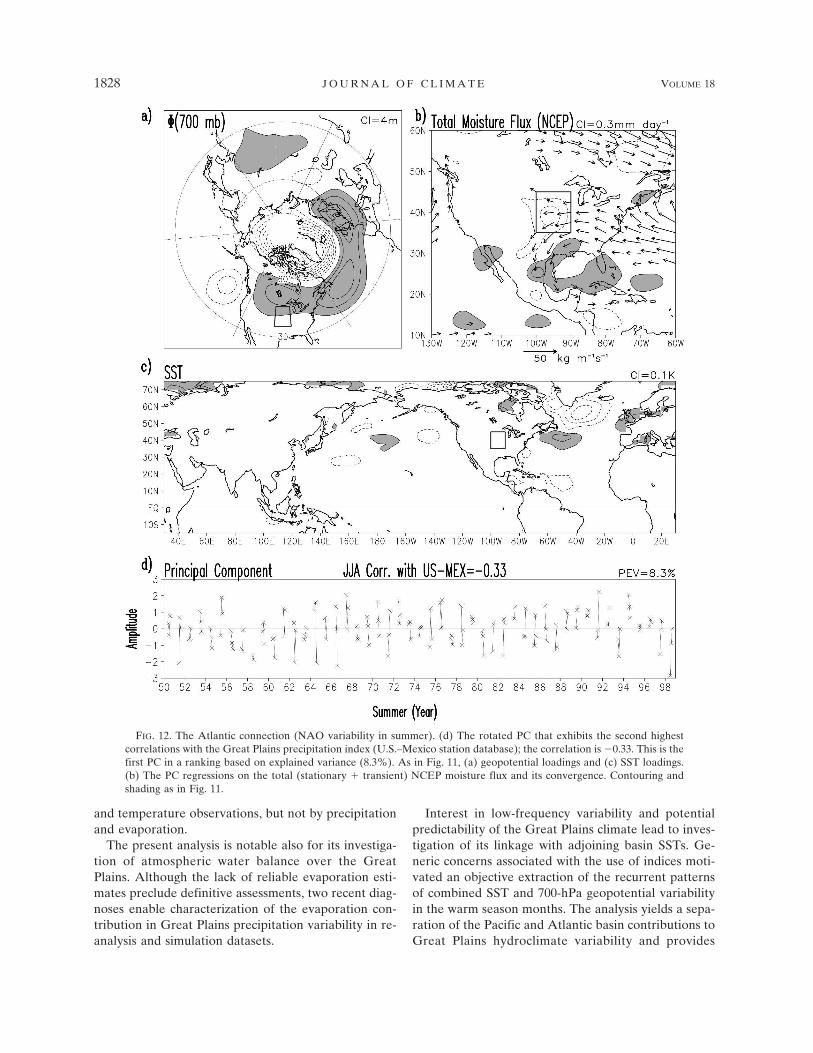
The rotated principal component that exhibits thesecond highest correlation (�0.33) with the GPP indexis shown in Fig. 12. This is the leading mode of com-bined variability and represents the North Atlantic Os-cillation (NAO) variability in summer. The SST load-ings are confined to the northern basin but the circula-tion anomalies are well extended both westward (up toand beyond the Great Plains) and eastward. The com-bined pattern compares favorably with the second-leading pattern in Lanzante’s warm season analysis(1984; Fig. 4b). There is little evidence, however, of anytrends in the PC distribution, quite unlike the case inwinter when the NAO PC exhibits an upward trendsince, at least, the early 1970s (Hurrell 1995; Figs. 9aand 12 of Nigam 2003). The warm season PC is, in fact,dominated by intraseasonal variability as its signchanges in 30 of the 49 summers. The contemporaneouscorrelation with NOAA/CPC’s NAO index (see onlineat http://www.cpc.ncep.noaa.gov/data/teledoc/nao.html) in June and July is �0.85.

The moisture fluxes associated with this mode areshown in the Fig. 12a; the vertically integrated fluxesover the United States are dominated by the stationarycomponent in the lower troposphere. The westwardfluxes across the eastern United States track the south-ern flank of the zonally extended ridge in Fig. 12a. Thisentire feature, including its North American center, ex-hibits vertical coherence and thus represents a north-ward shift of the Bermuda high. Examination of thelevel-by-level fluxes (not shown) indicates significantinteraction with North American orography, which

splits the westward fluxes in the lower troposphere intonorthwestward and southwestward streams; the latterbeing stronger. Interestingly, there is little hint of atrough over the Gulf of Mexico in Fig. 12a. The south-ward fluxes over the southern-tier states, of course, op-pose the climatological low-level jet that transportsphenomenal amounts of moisture northward from theGulf of Mexico. The limited impact of this mode onGreat Plains precipitation (�11% of the monthly sum-mer variance) is somewhat surprising in view of itslarge-scale, coherent structure.

The PC is strongly positive in at least two of the threemonths during the 1955, 1964, 1967, 1972, 1976, 1983,1990, and 1994 summers. Comparisons with Fig. 3a in-dicates that three of these eight summers (1955, 1976,and 1983) were, in fact, dry over the Great Plains. Theagreement with observations is even better when thePC is strongly negative (1958, 1993, and 1998)—allthree being wet summers.

6. Concluding remarks

The study has sought to ascertain the structure ofwarm season hydroclimate variability over the U.S.Great Plains—a region of profound importance forU.S. agriculture—and the extent to which the observedvariability features are represented in the state-of-the-art climate simulations. Interannual variability is thefocus here because its spatiotemporal structure isknown with less certainty than the seasonal cycle’s inboth climate observations and simulations. Analysis ofinterannual variability is thus more exciting and, per-haps, also more important in context of model assess-ments since model simulations are less scripted in theinterannual range; models are typically tuned using ob-served seasonal variability. The analysis is confined tothe latter half of the twentieth century (1950–98) forreasons of circulation data availability, and as such ex-cludes the devastating dust bowl years (1930s). Theanalyzed period however does include other notable,but shorter duration, dry (1952–55, 1976, 1983–84, 1988,1992) and wet (1951, 1981, 1993, 1998) summer spells.

The analysis strategy is precipitation centric, and re-volves around the Great Plains precipitation index. Un-like previous studies, the GPP index is objectively con-structed on the basis of the standard deviation distri-bution of monthly precipitation in the warm seasonmonths (section 3). The index derived from the U.S.–Mexico station precipitation dataset is taken to be the“gold standard,” and its structure and regressions arethe target for NCAR and NASA AMIP simulations,and also NCEP and ERA-40 reanalyses. Hydroclimatevariability in the reanalyses is not assured to be realisticas the reanalysis procedure is constrained by circulation


and temperature observations, but not by precipitationand evaporation.

The present analysis is notable also for its investiga-tion of atmospheric water balance over the GreatPlains. Although the lack of reliable evaporation esti-mates preclude definitive assessments, two recent diag-noses enable characterization of the evaporation con-tribution in Great Plains precipitation variability in re-analysis and simulation datasets.

Interest in low-frequency variability and potentialpredictability of the Great Plains climate lead to inves-tigation of its linkage with adjoining basin SSTs. Ge-neric concerns associated with the use of indices moti-vated an objective extraction of the recurrent patternsof combined SST and 700-hPa geopotential variabilityin the warm season months. The analysis yields a sepa-ration of the Pacific and Atlantic basin contributions toGreat Plains hydroclimate variability and provides

FIG. 12. The Atlantic connection (NAO variability in summer). (d) The rotated PC that exhibits the second highestcorrelations with the Great Plains precipitation index (U.S.–Mexico station database); the correlation is �0.33. This is thefirst PC in a ranking based on explained variance (8.3%). As in Fig. 11, (a) geopotential loadings and (c) SST loadings.(b) The PC regressions on the total (stationary � transient) NCEP moisture flux and its convergence. Contouring andshading as in Fig. 11.


leads for future investigation of the interaction path-ways and mechanisms.

The main findings on the structure and nature ofwarm season interannual variability of Great Plains hy-droclimate are as follows:

• Precipitation variability in the reanalysis data is quasirealistic: ERA-40 underestimates the variability am-plitude while NCEP overestimates it, both by �25%.ERA-40 variations are temporally better correlatedwith observations (0.71) than NCEP’s (0.53); NCEPand ERA-40 indices are correlated at 0.77.

• Models produce a realistic amplitude of precipitationvariability. The evolution is problematic, though,with simulated indices being temporally uncorrelatedwith the observed monthly GPP index: CAM’s cor-relation is 0.11, while NSIPP’s is �0.09.

• Convective and stratiform components of GreatPlains precipitation are very unequal in model simu-lations: The stratiform component is nearly zero inboth NSIPP and CAM models, whereas the two com-ponents are comparable in the ERA-40 dataset.

• Vertically integrated moisture fluxes linked withGreat Plains precipitation variability are broadlysimilar in the two reanalysis: Stationary fluxes are atleast 5 times larger than the transient ones over theGreat Plains, but flux convergences differ by only afactor of 2. ERA-40 fluxes (and convergence) are,however, stronger than NCEP’s by as much as 50%.The reanalysis differences are even bigger over theGulf of Mexico and Caribbean Sea where ERA-40has robust westward fluxes, which track the southernflank of a coherent anticyclonic circulation that pumpsmoisture northward from the Gulf. Aspects of thisflow feature are absent in the NCEP moisture fluxes.

• Moisture fluxes linked with Great Plains precipita-tion variability are quite realistic in the NSIPP simu-lation, being closer to ERA-40 than NCEP. CAMfluxes are however more like NCEP’s than ERA-40’s.

• Moisture flux convergence accounts for nearly all ofthe Great Plains precipitation anomaly in ERA-40,but not in NCEP reanalysis and model simulations.Convergent fluxes explain less than half of the pre-cipitation signal in the latter.

• Reanalysis evaporation anomalies over the GreatPlains are, apparently, as far apart as the two diag-nosed estimates. The NCEP anomaly ranges from 0.1to 0.3 mm day�1—not unlike the GOLD estimates—while the ERA-40 anomaly is not even up to thecontouring threshold (0.1 mm day�1), much like theCPC-based estimate.

• Evaporation anomalies linked with Great Plains pre-cipitation variations are phenomenally strong in

model simulations, reaching 1.2 mm day�1. Verylarge local evaporation in the models—up to 4 timeslarger than the highest observationally constrainedestimate (NCEP’s)—suggests a very different view ofthe anomalous atmospheric water budget; one inwhich local water sources (precipitation recycling)contribute overwhelmingly to precipitation variabil-ity. Model evaporation anomalies are clearly outliers.

• Rotated principal component analysis suggests a Pa-cific link with Great Plains hydroclimate variability,but the linkage mechanism remains to be elucidated;especially, the potential of concurrent/precursor SSTanomalies in the central/eastern tropical Pacific. TheAtlantic connection, on the other hand, is evidentlythrough NAO’s influence on the Bermuda high, andthe resulting interaction of circulation with North Am-erican orography; all of which serve to modulate thelow-level moisture transports from the Gulf of Mexico.

The study suggests the considerable importance of re-mote water sources (moisture fluxes) in generation ofGreat Plains hydroclimate variability. Getting the in-teraction pathways right is presently challenging formodels. Regional hydroclimate simulations and predic-tions will remain unattainable until models realisticallyrepresent the connectivity with remote regions, (i.e.,teleconnections). Models currently place a premium onlocal water sources (precipitation recycling) duringwarm season variability. Rapid recycling of precipita-tion must, however, require substantial input of energyinto the regional land surface. Investigation of this is-sue, especially, the role of cloudiness, has been initiatedin order to improve understanding of the water andenergy cycles over the U.S. Great Plains.

Acknowledgments. The authors would like to ac-knowledge support of NOAA/PACS GrantN A 0 6 G P 0 3 6 2 , D O E – C C P P G r a n t D E F G0201ER63258, and NSIPP Grant NAG512417. We ac-knowledge helpful discussions with Mathew Barlow,Ernesto Berbery, Paul Dirmeyer, Hugh van den Dool,Renu Joseph, Adam Schlosser, and Siegfried Schubert.Bob Dickinson and Aiguo Dai offered comments andsuggestions on improving the manuscript. We thankMarty Hoerling, Glenn White, and an ananymous re-viewer for their constructive input. Phil Pegion andMichael Kistler assisted with the NSIPP data extraction.

REFERENCES

Amador, J., and Coauthors, cited 2004: North American MonsoonExperiment (NAME): Science and implementation plan.NAME Project Science Team. [Available online at http://www.cpc.ncep.noaa.gov/products/precip/monsoon/.]

Barlow, M., S. Nigam, and E. H. Berbery, 1998: Evolution of theNorth American monsoon system. J. Climate, 11, 2238–2257.

——, ——, and ——, 2001: ENSO, Pacific decadal variability, and


U.S. summertime precipitation, drought, and streamflow. J.Climate, 14, 2105–2128.

Bell, G. D., and J. E. Janowiak, 1995: Atmospheric circulationassociated with the Midwest floods of 1993. Bull. Amer. Me-teor. Soc., 76, 681–695.

Dai, A., 2001: Global precipitation and thunderstorm frequencies. PartI: Seasonal and interannual variations. J. Climate, 14, 1092–1111.

——, and K. E. Trenberth, 2004: The diurnal cycle and its depiction inthe Community Climate System Model. J. Climate, 17, 930–951.

Dirmeyer, P. A., and L. Tan, 2001: A multi-decadal global land-surfacedataset of state variables and fluxes. COLA Tech. Rep. 102, 43 pp.[Available from the Center for Ocean–Land–Atmosphere Stud-ies, 4041 Powder Mill Road, MB 302, Calverton, MD 20705.]

——, X. Gao, and T. Oki, 2002: GSWP-2: The Second Global SoilWetness Project Science and Implementation Plan. IGPO Publica-tion Series, Vol. 37, International GEWEX Project Office, 65 pp.

Gates, W. L., and Coauthors, 1999: An overview of the results ofthe Atmospheric Model Intercomparison Project (AMIP I).Bull. Amer. Meteor. Soc., 80, 29–56.

Heideman, K. F., and J. M. Fritsch, 1988: Forcing mechanisms andother characteristics of significant summertime precipitation.Wea. Forecasting, 3, 115–130.

Higgins, R., Y. Chen, and A. Douglas, 1999: Interannual variabil-ity of the North American warm season precipitation regime.J. Climate, 12, 653–680.

Hornberger, G. M., and Coauthors, 2001: A plan for a new scienceinitiative on the global water cycle. U.S. Global Change Re-search Program Report, Washington, DC, 118 pp. [Availableonline at http://www.usgcrp.gov/usgcrp/Library/watercycle/wcsgreport2001/default.htm.]

Hu, Q., and S. Feng, 2001: Climatic role of the southerly flow fromthe Gulf of Mexico in interannual variations in summer rain-fall in the central United States. J. Climate, 14, 3156–3170.

Huang, J., H. M. Van den Dool, and K. P. Georgarakos, 1996:Analysis of model-calculated soil moisture over the UnitedStates (1931–1993) and applications to long-range tempera-ture forecasts. J. Climate, 9, 1350–1362.

Hulme, M., cited 1999: Global Monthly Precipitation, 1900–1999(Hulme). ORNL DAAC dataset. [Available online at http://www.daac.ornl.gov.]

Hurrell, J., 1995: Decadal trends in the North Atlantic Oscillation:Regional temperatures and precipitation. Science, 269, 676–679.

Janowiak, J. E., A. Gruber, C. R. Kondragunta, R. E. Livezey, and G.J. Huffman, 1998: A comparison of the NCEP–NCAR reanalysisprecipitation and the GPCP rain gauge–satellite combined datasetwith observational error considerations. J. Climate, 11, 2960–2979.

Kalnay, E., and Coauthors, 1996: The NCEP/NCAR 40-Year Re-analysis Project. Bull. Amer. Meteor. Soc., 77, 437–471.

Koster, R. D., M. J. Suarez, R. W. Higgins, and H. M. Van denDool, 2003: Observational evidence that soil moisture varia-tions affect precipitation. Geophys. Res. Lett., 30, 1241,doi:10.1029/2002GL016571.

Lanzante, J. R., 1984: A rotated eigenanalysis of the correlationbetween 700 mb heights and sea surface temperatures in thePacific and Atlantic. Mon. Wea. Rev., 112, 2270–2280.

Lau, K.-M., and H. Weng, 2000: Remote forcing of U.S. summer-time droughts and floods by the Asian monsoon? GEWEXNews, 10, 5–6.

Liu, A. Z., M. Ting, and H. Wang, 1998: Maintenance of circula-tion anomalies during the 1988 drought and 1993 floods overthe United States. J. Atmos. Sci., 55, 2810–2832.

Mo, K. C., J. Nogues-Paegle, and J. Paegle, 1995: Physical mecha-nisms of the 1993 summer floods. J. Atmos. Sci., 52, 879–895.

——, ——, and W. R. Higgins, 1997: Atmospheric processes as-sociated with summer floods and droughts in the centralUnited States. J. Climate, 10, 3028–3046.

Namias, J., 1966: Nature and possible causes of the northeasternUnited States drought during 1962–65. Mon. Wea. Rev., 94,543–554.

——, 1983: Some causes of United States drought. J. Appl. Me-teor., 22, 30–39.

——, 1991: Spring and summer 1988 drought over the contiguousUnited States—Causes and prediction. J. Climate, 4, 54–65.

Nigam, S., 2003: Teleconnections. Encyclopedia of AtmosphericSciences, J. R. Holton, J. A. Pyle, and J. A. Curry, Eds.,Academic Press, 2243–2269.

——, and H.-S. Shen, 1993: Structure of oceanic and atmosphericlow-frequency variability over the tropical Pacific and IndianOceans. Part I: COADS observations. J. Climate, 6, 657–676.

——, M. Barlow, and E. H. Berbery, 1999: Pacific decadal SSTvariability: Impact on U.S. drought and streamflow. Eos,Trans. Amer. Geophys. Union, 80, 621–625.

Prohaska, J. T., 1976: A technique for analyzing the linear rela-tionships between two meteorological fields. Mon. Wea. Rev.,104, 1345–1353.

Rayner, N. A., E. B. Horton, D. E. Parker, C. K. Folland, andR. B. Hackett, 1996: Version 2.2 of the global sea-ice and seasurface temperature dataset, 1903–1994. Hadley Centre Tech.Note CRTN 74, 21 pp. [Available from Hadley Centre, MetOffice, London Road, Bracknell RS12 2SY, United Kingdom.]

——, D. E. Parker, E. B. Horton, C. K. Folland, L. V. Alexander,D. P. Rowell, E. C. Kent, and A. Kaplan, 2003: Global analy-ses of sea surface temperature, sea ice, and night marine airtemperature since the late nineteenth century. J. Geophys.Res., 108, 4407, doi:10.1029/2002JD002670.

Reynolds, R. W., N. A. Rayner, T. M. Smith, D. C. Stokes, and W.Wang, 2002: An improved in situ and satellite SST analysisfor climate. J. Climate, 15, 1609–1625.

Ruiz-Barradas, A., J. A. Carton, and S. Nigam, 2000: Structure ofinterannual-to-decadal climate variability in the tropical At-lantic sector. J. Climate, 13, 3285–3297.

Schubert, S. D., M. J. Suarez, P. Pegion, R. J. Koster, and J. T.Bacmeister, 2004: Causes of long-term drought in the U.S.Great Plains. J. Climate, 17, 485–503.

Ting, M., and H. Wang, 1997: Summertime U.S. precipitation vari-ability and its relation to Pacific sea surface temperature. J.Climate, 10, 1853–1873.

Trenberth, K. E., 1990: Recent observed interdecadal climatechanges in the Northern Hemisphere. Bull. Amer. Meteor.Soc., 71, 988–993.

——, and C. J. Guillemot, 1996: Physical processes involved in the1988 drought and 1993 floods in North America. J. Climate, 9,1288–1298.

——, G. W. Branstator, and P. A. Arkin, 1988: Origins of the 1988North American drought. Science, 242, 1640–1645.

Wallace, J. M., and D. S. Gutzler, 1981: Teleconnections in thegeopotential height field during the Northern Hemispherewinter. Mon. Wea. Rev., 109, 784–812.

Xie, P., and P. A. Arkin, 1997: Global precipitation: A 17-yearmonthly analysis based on gauge observations, satellite esti-mates, and numerical model outputs. Bull. Amer. Meteor.Soc., 78, 2539–2558.

Xie, S.-P., and Y. Tanimoto, 1998: A pan-Atlantic decadal climateoscillation. Geophys. Res. Lett., 25, 2185–2188.

Xue, Y., P. J. Sellers, J. L. Kinter, and J. Shukla, 1991: A simplifiedbiosphere model for global climate studies. J. Climate, 4, 345–364.


Documents

Warm Season Rainfall Variability over the U.S. Great