Embed Size (px)
Citation preview

Master Thesis in Statistics and Data Mining
Warranty claims analysis for household appliances produced by ASKO
Appliances AB
Ana Turk
Copyright
The publishers will keep this document online on the Internet - or its possible replacement -
for a considerable time from the date of publication barring exceptional circumstances.
The online availability of the document implies a permanent permission for anyone to read,
to download, to print out single copies for your own use and to use it unchanged for any
non-commercial research and educational purpose. Subsequent transfers of copyright cannot
revoke this permission. All other uses of the document are conditional on the consent of the
copyright owner. The publisher has taken technical and administrative measures to assure
authenticity, security and accessibility.
According to intellectual property law the author has the right to be mentioned when his/her
work is accessed as described above and to be protected against infringement.
For additional information about the Linköping University Electronic Press and its
procedures for publication and for assurance of document integrity, please refer to its WWW
home page: http://www.ep.liu.se/
© Ana Turk
Abstract
The input collected from warranty claims data links customer feedback with product quality.
Results from warranty claim analysis can potentially improve product quality, customer
relationships and positively affect business. However working on warranty claims data
holds many challenges that requires a significant share of time devoted to data cleaning and
data processing.
The purpose of warranty claims analysis is to get the comprehensive overview of the
reliability, costs and quality of household appliances produced by ASKO. While there are
different ways to approach this problem, we will focus on non-parametric and semi-
parametric methods, by using Kaplan-Meier estimators and Cox proportional hazard model
respectively. These kinds of models are time dependent and therefore used for prediction of
household appliance reliability. Even though non-parametric models are quite informative
they cannot handle additional characteristics about observable product hence the semi-
parametric Cox proportional hazard model was proposed. Apart from the reliability analysis,
we will also predict warranty costs with probit model and observe inequality in household
appliances part failures as a part of quality control analysis. Described methods were
selected due to the fact that the warranty claims analysis will be practiced in future by
ASKO’s quality department and therefore straight forward methods with very informative
results are needed.

Acknowledgements
I would like to thank ASKO for providing data and Magnus Älmegran, Antonio Scarlini,
Simon Kumer and Marko Šefer for making this cooperation possible.
I would also like to thank my supervisor Bertil Wegmann for guiding and supporting me
throughout this research. However I would not be able to come so far without a guidance of
all professors in the Statistics and Data Mining department at Linköping University.
Last but not least I would like to thank my family and friends for being there for me and
supporting me on this path. My mom Suzana Turk and dad Karol Turk made this study
possible and I will be always grateful to them for supporting me in all my life decisions. The
one person that always listens and cares about me unconditionally is my sister Ines Turk and
even though I do not say it enough I am really thankful to have you in my life.
LIU-IDA/STAT-A--13/005--SE
Ana Turk
Linköping University
2013-06-17
Table of Contents
Abstract .................................................................................................................................... 3
Acknowledgements .................................................................................................................. 4
Table of Contents ...................................................................................................................... 5
1 Introduction ....................................................................................................................... 1
1.1 Background ................................................................................................................. 2
1.2 Objectives ................................................................................................................... 4
2 Data ................................................................................................................................... 4
2.1 Variables...................................................................................................................... 5
2.2 Raw data ..................................................................................................................... 7
2.3 Secondary data ............................................................................................................ 8
2.4 Univariate analysis ...................................................................................................... 9
3 Methods ........................................................................................................................... 15
3.1 Reliability analysis for a singular failure .................................................................. 16
3.1.1 Reliability function ............................................................................................ 16
3.1.2 Hazard function .................................................................................................. 17
3.1.3 Kaplan-Meier estimator ..................................................................................... 17
3.1.4 Cox proportional hazard model ......................................................................... 18
3.2 Reliability analysis for multiple failures .................................................................. 20
3.2.1 Marginal Cox model for multiple failures ......................................................... 20
3.3 Part failure analysis ................................................................................................... 21
3.3.1 Pareto principle .................................................................................................. 21
3.3.2 Gini coefficient .................................................................................................. 22
3.4 Warranty cost analysis .............................................................................................. 24
3.4.1 Probit model ....................................................................................................... 24
4 Results ............................................................................................................................. 25
4.1 Reliability analysis for a single failure ..................................................................... 25
4.1.1 Testing proportional hazard assumptions ........................................................... 25
4.1.2 Kaplan-Meier estimator ..................................................................................... 27
4.1.3 Cox proportional hazard model ......................................................................... 28
4.2 Reliability analysis for multiple failures .................................................................. 30
4.2.1 Marginal Cox model for multiple failures ......................................................... 30
4.3 Part failure................................................................................................................. 33
4.4 Warranty cost analysis .............................................................................................. 34
4.4.1 Probit model ....................................................................................................... 34
5 Conclusion and discussion .............................................................................................. 35
6 Future work ..................................................................................................................... 39
7 Literature ......................................................................................................................... 41
Appendix A............................................................................................................................. 45
Appendix B............................................................................................................................. 47
Index of Tables
Table 1: Summary of Warranty claims data ................................................................................................................ 7 Table 2: Proportional hazard assumption testing for part failure ...............................................................................26 Table 3: Cox proportional hazard output ....................................................................................................................28 Table 4: Multiple failure marginal Cox model results .................................................................................................30 Table 5: Summary of Backward elimination ...............................................................................................................31 Table 6: Multiple failure marginal Cox model results after the backward elimination ................................................32 Table 7: Model Fit Statistics .......................................................................................................................................32 Table 8: Gini coefficient output ..................................................................................................................................33 Table 9:Probit regression model output .....................................................................................................................34 Table 10: Marginal effect for probit regression model ...............................................................................................35
Index of Figures
Figure 1: Data for one-dimensional non-renewing warranty (Blischke et.al., 2011) .................................................... 5 Figure 2: Data for analysis .......................................................................................................................................... 6 Figure 3: The distribution of a life time for Dishwashers ............................................................................................. 9 Figure 4: The distribution of a life time for washing machines ...................................................................................10 Figure 5: The distribution of a life time for tumble dryers ..........................................................................................11 Figure 6: Bar chart presenting the percentage of failures for dishwashers, washing machines and tumble dryers. ....12 Figure 7: Bar chart presenting extreme number of failures for dishwashers, washing machines and tumble dryers. .12 Figure 8: Line plot of cumulative average costs regarding the number of failures for Dishwashers, Washing machines
and Tumble dryers ............................................................................................................................................13 Figure 9: Bar chart of 10 most frequent part failures .................................................................................................14 Figure 10: Pareto rule applied to part failures within warranty period .......................................................................22 Figure 11: A modified Lorenz curve for part failure analysis .......................................................................................23 Figure 12: Kaplan-Meier curves for testing the proportionality of explanatory variables ...........................................26 Figure 13: Kaplan-Meier survival curves estimates for Washing machines, Tumble dryers and Dishwashers .............27 Figure 14: Predicted survival curve based on Cox PH model for dishwashers .............................................................29 Figure 18: Lorenz curve presenting the inequality of the part failure distribution ......................................................33
1
1 Introduction
Survival analysis plays an important role in medicine data and biostatistics but its
characteristics can be applied to the field of warranty analysis as well, where it is mostly
known as reliability analysis. Both fields focus on the lifetime of observable units but
instead of for example survival of bacteria we observe the reliability of household
appliances.
Reliability of a product is related to the dependability, successful operation or performance
and the absence of a failure (Blischke et.al, 2011). Considering the life cycle of the product
we can observe different stages of its reliability. It starts with design reliability, inherent
reliability, reliability at sale and once the product is sold we can observe field reliability
(Blischke et.al, 2011). We will focus on field reliability where performance of a product will
be evaluated regarding different factors (model type, severity of failures and working
power).
What makes reliability analysis special is data censoring since additional information about
the item future can be incorporated in different models. Lifetime of each item is observed
for a certain period of time and after that if no failures are reported it becomes censored.
The observable lifetime period can either be censored after the last noted failure of specific
household appliance or after the warranty time expires in case when no failures are
presented.
There are many reasons that impel us to explore the field of warranty analysis. This problem
concerns the marketing (sales), economic (cost), engineering (design) and operational
(servicing) aspects of a company (Murthy and Djamaludin, 2002). An important segment of
warranty claims analysis is repair costs hence, cost analysis will be presented hereafter.
Pareto analysis will be applied as a part of statistical quality control. With the aim of
identifying a few of the most important quality problems we can use different methods that
focus on part failure inequality. These quality issues correspond to the parts of household
appliances that cause the most failures and are therefore most frequently presented in
2
warranty claims data.
The purpose of this thesis is to find appropriate models for warranty claims data where the
reliability of household appliances, quality control and the costs of warranty claims are
evaluated.
This thesis is divided in six parts. In the first part we describe the background of warranty
analysis and shortly present the ASKO company. The thesis objectives will be specified in
the first part as well. In the second part we present the characteristics and issues of warranty
data and present the data used for the further analysis. In the third part we present the
methods that will be used for analysis. Results are presented in the fourth part. After that,
the conclusion including evaluation of the methods used will be presented in the fifth part.
Future work will be presented in the final sixth part of this thesis.
1.1 Background
Warranty is defined as a contractual obligation of a manufacturer in selling a product to
ensure the product functions properly during the warranty period (Blischke et al., 2011).
Customers need assurance that a product will perform satisfactory over its designed useful
life (Blischke et al., 2011).
Processing and analysing warranty claims data will be in special benefit for ASKO since
they are dealing with the warranty claims on a daily basis. ASKO is an internationally
oriented Swedish company with long tradition in production of household appliances.
General warranty policy in ASKO is two year non-renewing warranty. For this time period
ASKO replaces or repairs the defected parts and finances the labour needed. Two years
warranty policy considered in this thesis is only eligible for ASKO’s distributors. Even
though the warranty period for customers can be longer and it is usually up to 5 years long,
all the additional warranty expenses after two years become a distributor’s responsibility.
ASKO’s warranty policy only depends on the time, not for instance mileage or usage as it is
common for automotive industry. Therefore we can refer to our data as one dimensional
3
data. Another characteristic of our warranty policy is that it is non-renewing which means
that the warranty term does not begin anew on replacement or repair of a failed item
(Blischke et al., 2011).
Warranty analysis is beneficial for a company because it can give a better overview of the
product quality. Through the reengineering of management processes and the application of
a suitable warranty model, it is possible to (Diaz et al., 2010):
• Improve sales of extended warranties and additional related products.
• Improve quality by improving the information flow about product defects and their
sources.
• Improve customer relationships.
• Reduce expenses related to warranty claims and data processing.
• Better management and control over the warranty costs.
• Reduce invalid expenses and other warranty costs.
Moreover the ability to predict and estimate failures for warranty period makes it possible to
appropriately size the necessary resources and consequently optimize the costs (Patankar et
al., 1995). The optimal warranty time should be considered in terms of the relationship
between the price and the warranty policy (Kotler, 1976; Peterson, 1970).
Product performance depends on the reliability of the product, which in turn, depends on
decisions made during its design, development and production (Blischke et al., 2011).
Therefore we will focus on the problem of product reliability that conveys the concept of
dependability, successful operation or performance and the absence of failures. It is an
external property of great interest to both manufacturer and consumer (Blischke et al.,
2011). The main purpose of warranty analysis is therefore customer satisfaction and product
reliability.
4
1.2 Objectives
Firstly we want to estimate the probability of product failure within the two year warranty
period for each household appliance to get a better overview of the warranty period. By that
we would like to reconsider the length of the warranty period for ASKO’s household
appliances.
Secondly we would like to identify the most frequent warranty events (failures) to discover
the most unreliable parts that influence the proper functioning of the household appliances.
This will present a first step in a household appliance quality control check for ASKO.
Lastly we would like to estimate warranty expenses for different products regarding the
repair and labour costs. This part is associated with warranty cost analysis and will give us a
deeper understanding of the projected warranty expenses.
2 Data
We will use warranty claims data that are collected daily by ASKO’s quality department.
Apart from the warranty claims data, total production of household appliances data will be
used as a supplementary data. The main reason for using supplementary data is to get
additional information about total number of household appliances that did not failed in the
two year warranty period. These data are incomplete in the sense that the period of
observation is terminated prior to the failure of all items under observation (Blischke et al.,
2011). Such characteristics are typical for censored data. Censoring is also present in
warranty claims data but it only applies to further failures after the last failure of the
household appliance.
Warranty data is known to be pretty messy and it is quite common to take into consideration
missing values, incomplete information, and unclear nature of data (Hagen et al., 2013).
These issues were presented in our database as well. For that reason a significant share of
time was devoted to data processing. To avoid these problems in the future a more organised
database would be advisable. This only applies for the variables that are crucial for
5
reliability analysis and unnecessary errors that appear when claims are added in the
database.
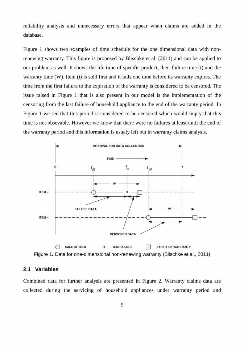
Figure 1 shows two examples of time schedule for the one dimensional data with non-
renewing warranty. This figure is proposed by Blischke et al. (2011) and can be applied to
our problem as well. It shows the life time of specific product, their failure time (t) and the
warranty time (W). Item (i) is sold first and it fails one time before its warranty expires. The
time from the first failure to the expiration of the warranty is considered to be censored. The
issue raised in Figure 1 that is also present in our model is the implementation of the
censoring from the last failure of household appliance to the end of the warranty period. In
Figure 1 we see that this period is considered to be censored which would imply that this
time is not obsevable. However we know that there were no failures at least until the end of
the warranty period and this information is usualy left out in warranty claims analysis.
Figure 1: Data for one-dimensional non-renewing warranty (Blischke et al., 2011)
2.1 Variables
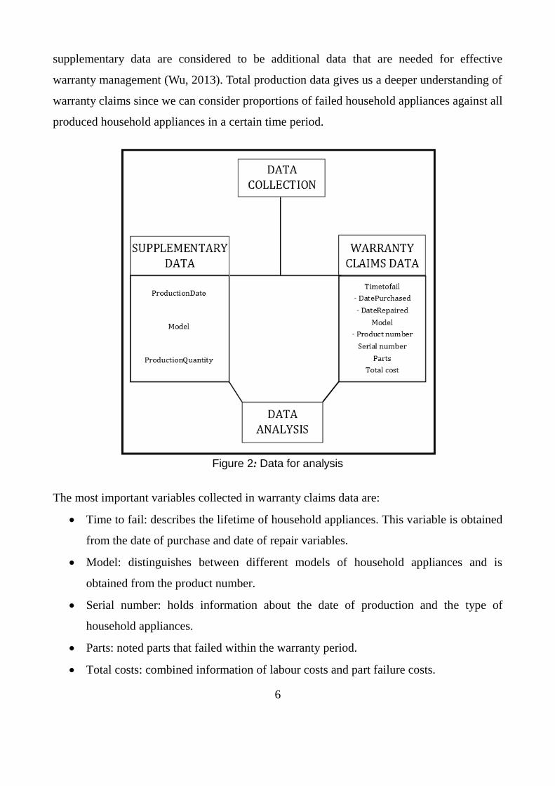
Combined data for further analysis are presented in Figure 2. Warranty claims data are
collected during the servicing of household appliances under warranty period and
6
supplementary data are considered to be additional data that are needed for effective
warranty management (Wu, 2013). Total production data gives us a deeper understanding of
warranty claims since we can consider proportions of failed household appliances against all
produced household appliances in a certain time period.
Figure 2: Data for analysis
The most important variables collected in warranty claims data are:
Time to fail: describes the lifetime of household appliances. This variable is obtained
from the date of purchase and date of repair variables.
Model: distinguishes between different models of household appliances and is
obtained from the product number.
Serial number: holds information about the date of production and the type of
household appliances.
Parts: noted parts that failed within the warranty period.
Total costs: combined information of labour costs and part failure costs.
7
Supplementary total production data include the following information:
Production date: time when household appliances was produced.
Model: distinguishes between different model types.
Production quantity: gives information about the quantity of household appliances
produced in certain time period.
2.2 Raw data
We will observe a two year time period of warranty claims for ASKO’s household
appliances. All household appliances included in the final database are purchased between
January 2009 and December 2010. The last noted repair for observed household appliances
is in December 2012, when the warranty expires for all of the observed household
appliances. Our observation ends with a day 730, which is the last day allowing no expenses
warranty policy for ASKO’s distributors.
Even though ASKO produces many different household appliances our analysis includes
only dishwashers, washing machines and tumble dryers. Considering different types of
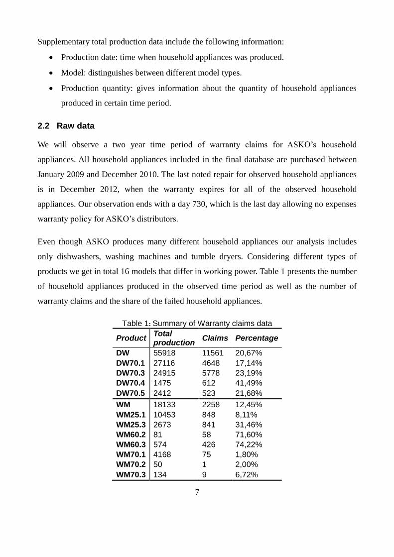
products we get in total 16 models that differ in working power. Table 1 presents the number
of household appliances produced in the observed time period as well as the number of
warranty claims and the share of the failed household appliances.
Table 1: Summary of Warranty claims data
Product Total production
Claims Percentage
DW 55918 11561 20,67%
DW70.1 27116 4648 17,14%
DW70.3 24915 5778 23,19%
DW70.4 1475 612 41,49%
DW70.5 2412 523 21,68%
WM 18133 2258 12,45%
WM25.1 10453 848 8,11%
WM25.3 2673 841 31,46%
WM60.2 81 58 71,60%
WM60.3 574 426 74,22%
WM70.1 4168 75 1,80%
WM70.2 50 1 2,00%
WM70.3 134 9 6,72%
8
TD 18124 1997 11,02%
TD25.1 10764 904 8,40%
TD25.3 2433 668 27,46%
TD60.1 4286 56 1,31%
TD60.2 67 48 71,64%
TD60.3 574 321 55,92%
Sum 92175 15816 17,16%
In total there were 92175 household appliances produced for the United States (US) market
from the beginning of January 2009 to the end of December 2010. In this time period 15816
warranty claims were recorded which gives us app. 17% overall failure of household
appliances.
2.3 Secondary data
Some additional variables needed to be produced for the purpose of reliability and cost
analysis. The first variable added was time to failure (Timetofail in the Figure 2) which
describes the life time of specific product. Moreover translation from product number in
warranty claims data to the fitting household appliance type through “translation between
code systems” database was needed to get all possible household appliances model types.
Dummy variables were formed from the model variable to distinguish between household
appliances (dish washers, tumble dryers and washing machines) working power.
Categorising the levels of working power, we have a high level and low level household
appliances. The low level household appliances are sold the most (DW70.1, WM70.1,
TD60.1 etc.) and usually less costly. The main difference between low level household
appliances and high level household appliances is control unit and its functionality. Low
level household appliances have in general fewer features than the high level household
appliances.
A severity of the failure (mild or no failure, severe failure) dummy variable was obtained
from parts variable. When considering the seriousness of the failure we distinguish between
no failure (for total production data without a failure) or mild failure where only labour
costs are considered and there is no need for part replacement and severe failure where parts

9
need to be replaced due to their inability to function properly.
2.4 Univariate analysis
To illustrate our data in detail we will present a description of each single variable and
perform a univariate analysis for the warranty claims data.
Time of failure
Time of failure is an important variable for the reliability analysis because it displays the life
time characteristics of the product. Distributions of this variable for each individual
household appliance are presented here.
Dishwashers
Figure 3: The distribution of a life time for Dishwashers
The distribution in Figure 3 appears to be skewed to the right. Hence the mean time
presented with a dashed line appears before the end of the first year which is the middle
10
value of the observable warranty time. This kind of distribution is frequently presented in
such cases and therefore expected. It results from small numbers of exceptionally long-lived
items (Blischke et al., 2011). We can see a peak in the first days of dishwashers’ usage in the
Figure 3. Moreover the first 300 days together present more than 50% (Appendix B) of
reported failures.
Washing machines
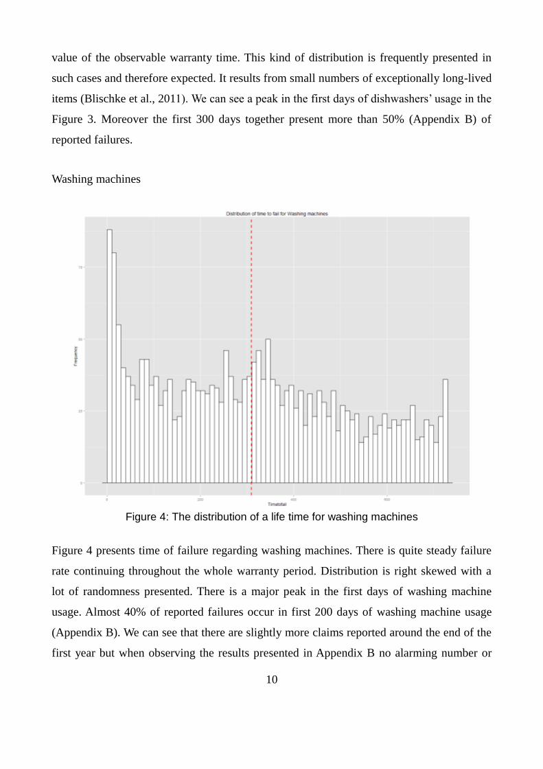
Figure 4: The distribution of a life time for washing machines
Figure 4 presents time of failure regarding washing machines. There is quite steady failure
rate continuing throughout the whole warranty period. Distribution is right skewed with a
lot of randomness presented. There is a major peak in the first days of washing machine
usage. Almost 40% of reported failures occur in first 200 days of washing machine usage
(Appendix B). We can see that there are slightly more claims reported around the end of the
first year but when observing the results presented in Appendix B no alarming number or
11
pattern for failed washing machines was found.
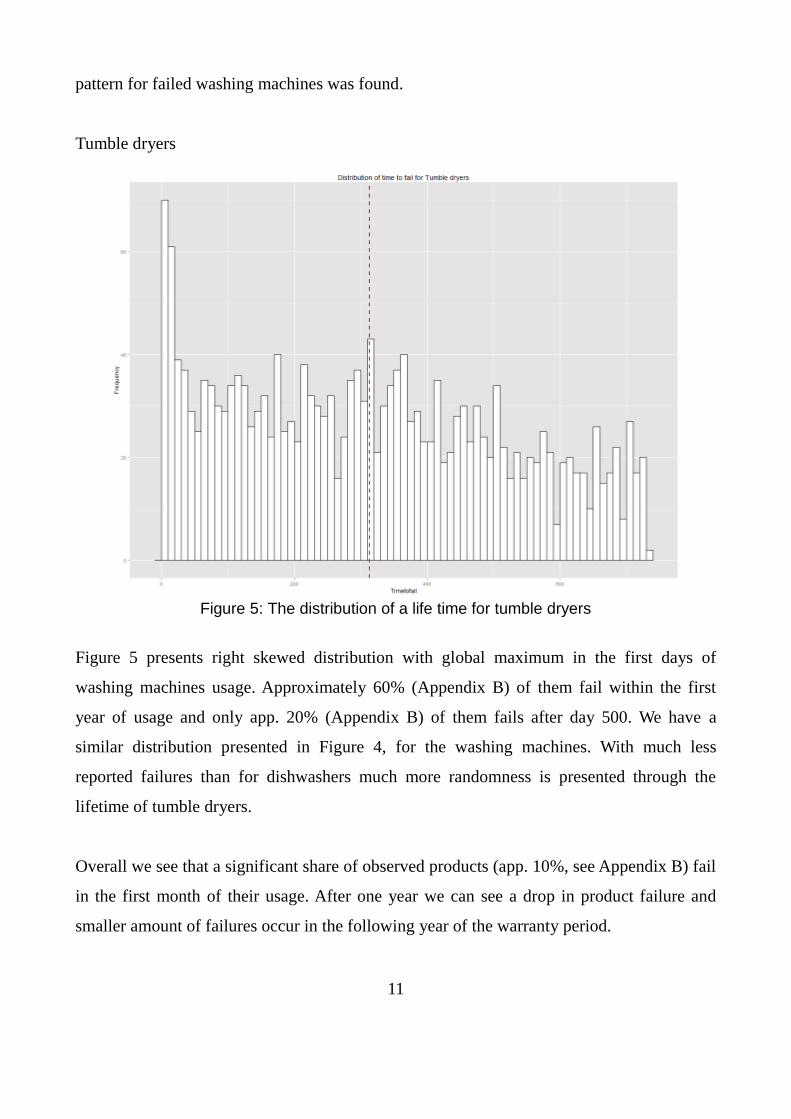
Tumble dryers
Figure 5: The distribution of a life time for tumble dryers
Figure 5 presents right skewed distribution with global maximum in the first days of
washing machines usage. Approximately 60% (Appendix B) of them fail within the first
year of usage and only app. 20% (Appendix B) of them fails after day 500. We have a
similar distribution presented in Figure 4, for the washing machines. With much less
reported failures than for dishwashers much more randomness is presented through the
lifetime of tumble dryers.
Overall we see that a significant share of observed products (app. 10%, see Appendix B) fail
in the first month of their usage. After one year we can see a drop in product failure and
smaller amount of failures occur in the following year of the warranty period.
12
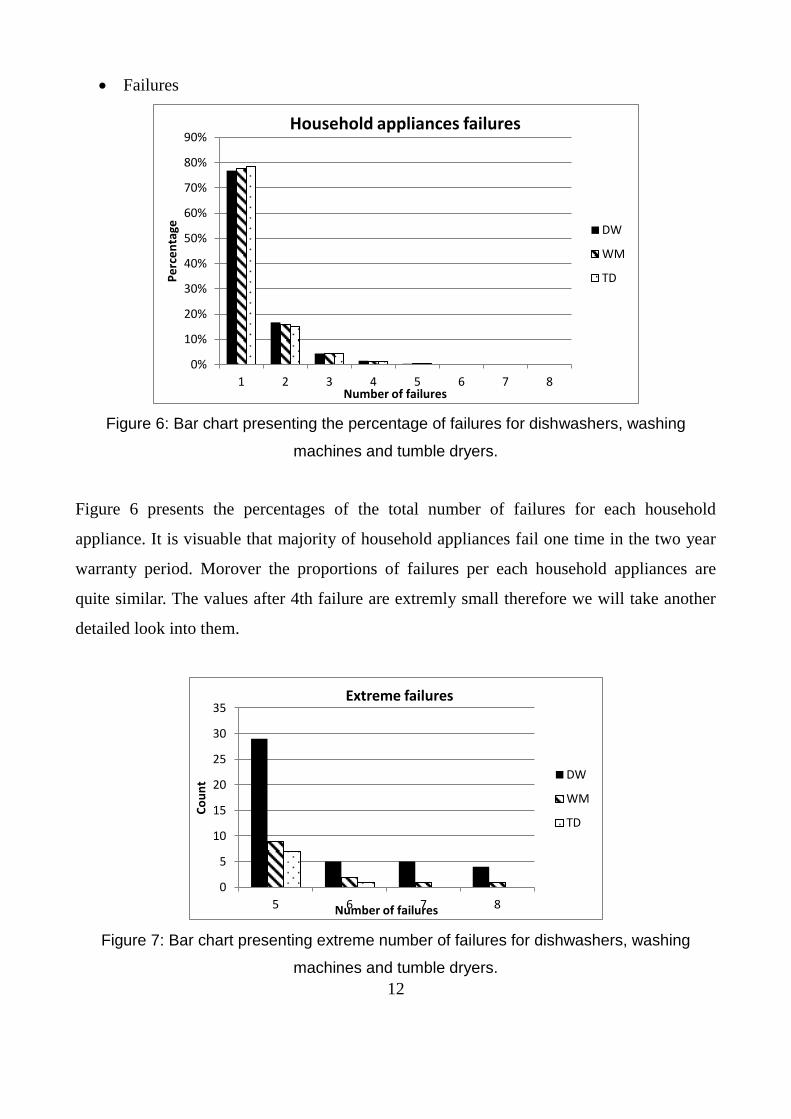
Failures
Figure 6: Bar chart presenting the percentage of failures for dishwashers, washing
machines and tumble dryers.
Figure 6 presents the percentages of the total number of failures for each household
appliance. It is visuable that majority of household appliances fail one time in the two year
warranty period. Morover the proportions of failures per each household appliances are
quite similar. The values after 4th failure are extremly small therefore we will take another
detailed look into them.
Figure 7: Bar chart presenting extreme number of failures for dishwashers, washing
machines and tumble dryers.
0%
10%
20%
30%
40%
50%
60%
70%
80%
90%
1 2 3 4 5 6 7 8
Pe
rce
nta
ge
Number of failures
Household appliances failures
DW
WM
TD
0
5
10
15
20
25
30
35
5 6 7 8
Co
un
t
Number of failures
Extreme failures
DW
WM
TD
13
In general dishwashers are best selling product in the US market and therefore some extrem
number of failures could be expected. However 42 of the observed dishwashers have
extreme value of failures which are first of all quite costly for ASKO and secondly
inconvenient for customers. Among the other observed household appliances we note that
only dishwashers and washing have 7 and 8 failures.
Observing the serial number for all of the failed product we notice that they have one
common feature. Most of them are produced before (2007, 2008) the year 2009. This gives
us a reason to believe that the time from household appliances production to purchase
(leverage time) is important when it comes to multiple product failures.
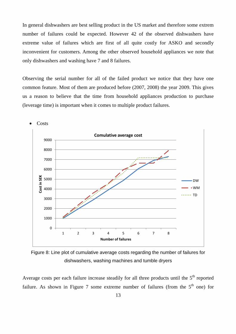
Costs
Figure 8: Line plot of cumulative average costs regarding the number of failures for
dishwashers, washing machines and tumble dryers
Average costs per each failure increase steadily for all three products until the 5th
reported
failure. As shown in Figure 7 some extreme number of failures (from the 5th
one) for
0
1000
2000
3000
4000
5000
6000
7000
8000
9000
1 2 3 4 5 6 7 8
Co
st in
SEK
Number of failures
Comulative average cost
DW
WM
TD
14
dishwashers and washing machines are present in the data and as we see in Figure 8 their
cumulative average failure costs exceeds the 7000 SEK. It is important to note that the
number of failures after the 5th
failure decreases considerably therefore the average costs are
just an approximations.
Part failure
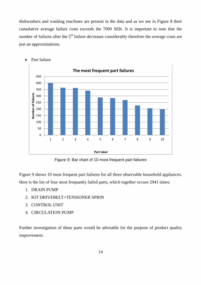
Figure 9: Bar chart of 10 most frequent part failures
Figure 9 shows 10 most frequent part failures for all three observable household appliances.
Here is the list of four most frequantly failed parts, which together occure 2941 times:
1. DRAIN PUMP
2. KIT DRIVEBELT+TENSIONER SPRIN
3. CONTROL UNIT
4. CIRCULATION PUMP
Further investigation of these parts would be advisable for the purpose of product quality
improvement.
0
50
100
150
200
250
300
350
400
450
1 2 3 4 5 6 7 8 9 10
Nu
mb
er
of
failu
res
Part label
The most frequent part failures
15
3 Methods
Much has been written about warranty analysis and warranty cost analysis (Blischke et al.,
2011). Apart from the usual parametric, non-parametric and semi-parametric methods used
for analysing the reliability of the product, Bayesian methodology was proposed by Percy
(2002). Estimation of model parameters by applying Poisson process was proposed by
Kulkarni and Resnick (2008) for investigation of risk management policy. Wu (2010)
presented a paper that considers human factor in warranty claims analysis which is not so
commonly presented in this field. Twisk et al. (2005) presents and compares naive and
longitudinal techniques for recurrent event data analysis. As a part of warranty analysis
there are a lot of different approaches for analysing warranty costs. Model for future costs
was proposed by Amato et al. (1976). Moreover time dependent costs were proposed by Ja
et al. (2001) and model for non-zero repair time was proposed by Chuckova and Hayakawa
(2004). These different approaches give us the feeling of variety of analysis proposed for
warranty claims data however the differences in data implementation and objectives need to
be considered in the model selection.
Since we are observing the life time of different household appliances reliability analysis is
one way to approach this problem. Reliability can be estimated parametrically, semi-
parametrically or non-parametrically. Semi-parametrical Cox proportional hazard model
will help us estimate the reliability of different household appliances regarding their
qualities and therefore estimate the probability of product failure within the two years
warranty period.
We will use different models for the purpose of meeting the objectives. These models are:
Non-parametric Kaplan-Meier model will help us estimate the probability of the
single failure of household appliances and therefore evaluate the reliability thereof.
Semi-parametrical model such as Cox proportional hazard model will be used for
deeper understanding of relations between the product failure and household
appliances characteristics. Furthermore marginal Cox model will be used for multiple
failures prediction model.
16
Pareto principle will be tested on part failures to get the overall view of the true part
failures that mostly corrupt the products quality.
Probit model will be used for warranty cost analysis to estimate the relationship
between the warranty costs and the products characteristic.
The reliability analysis, quality control analysis and cost analysis were done in SAS and
partly in R programme. For reliability analysis proc lifetest in SAS or survival library in R
can be used. Moreover ineq library in R can be used for inequality measurement of part
failures since it allows us to calculate Gini coefficient and get the visualization of Lorenz
curve. Probit analysis can be done with proc logistic in SAS or rms library in R.
3.1 Reliability analysis for a singular failure
As mentioned before reliability analysis uses parametric, non-parametric and semi-
parametric models for analysis. Even though parametric models were presented first in the
history of survival analysis, semi-parametric and non-parametric approaches turned out to
be more robust and due to the ability to overlook the exact underlying distribution of
survival times they became more popular (Smith et.al, 2011). The reason for that is that
parametric models such as Weibull, Exponential and Log-logistic need both the hazard
function and the effect of any covariates specification. As a result estimated survival curves
are smoother as they draw information from the whole data but the main drawback by
applying parametric methods is that they require extra assumption about distribution that
may not be appropriate (Kleinbaum and Klein, 2005). For this reason non-parametric and
semi-parametric models will be used here.
3.1.1 Reliability function
The reliability function R(t), also known as the survival function S(t) is defined as:
)(1)Pr()( tFtTtR
Where t is a specific point in time, T is the survival time and F(t) is failure probability.
17
Hence, the reliability function is the probability that the time of failure is later than some
specified time point t. The reliability function of the product R(t) is specified as (Blischke et
al., 2011):
non-increasing function of t, t0
1)0( R and 0)( R
3.1.2 Hazard function
Hazard function or the failure rate function gives us information about the risk of object
failing at time [t, t + ), given that it has not failed before the observable time t. The hazard
rate h(t) is defined as:
)(
)()|(lim)(
0 tR
tf
t
tTtFth
t
The hazard function assesses the instantaneous risk of demise at time t (Fox, 2002). With
the hazard function we obtain the probability that observable object will experience an event
at time t while it is at risk for having an event (ucla.edu, 2013). It is important to note that
the hazard rate is an un-observed variable and yet it controls both the occurrence and the
timing of the events (ucla.edu, 2013).
3.1.3 Kaplan-Meier estimator
We use the Kaplan-Meier estimator (“product-limit estimator”) for maximum likelihood
estimation of the survival time until the first failure. Kaplan-Meier estimation for the
survival function can be noted as (Kaplan and Meier, 1958):
1)(ˆ
ii
iii
Nn
NntR
Where ti is duration of study at point i, Ni is number of deaths up to the point i and ni is the
number of objects at risk just prior to ti. Even though this non-parametric method can only
estimate the survival curve for different groups of household appliances it allows to include
18
censored data and is therefore quite informative regardless its simplicity.
3.1.4 Cox proportional hazard model
Reliability modelling can be used to examine how the reliability function depends on one or
more predictors, usually termed as covariates (Fox, 2002). We use Cox Proportional Hazard
model (Cox PH model) for estimation of the hazard function which allows including
household appliances characteristics. The Cox PH model is widely used in survival and
reliability analysis due to its flexibility. Unlike parametric models in reliability analysis the
Cox PH model allows for modelling without any assumptions about the parametric
distribution of survival times (Smith et. al, 2011).
Proportional hazard assumption needs to be tested before applying the Cox PH model to the
data. Cox PH model assumes that hazards are proportional over time (Meadows et al.,
2006). When validating hazards, the hazard ratio is supposed to be constant over survival
time and no temporary bias is allowed to influence the endpoint (Smith et. al, 2011).
Therefore the changes in the hazard function of any subject over time will always be
proportional to changes in the hazard function of any other subject and to changes in the
underlying hazard function over time (Smith and Smith, 2004).
To test the proportional hazard assumptions we will use two frequently used tests; Log-rank
test and Wilcoxon test. The difference between those two tests is that Wilcoxon test puts
more weight on the early failures than the later one, whereas Log-rank test does not include
weighting of the failure time.
We are testing the following hypothesis:
H0: There is no difference among the survival curves
H1: There is a difference among the survival curves
The Cox proportional hazard regression model is defined by:
19
),...,exp()()|( 110 pp XXthXth
Where )|( Xth is the conditional hazard function at time t and )(0 th is the baseline hazard
function for the probability of failing when all of the explanatory variables are equal to zero.
Cox proportional hazard regression model is divided into two parts (Gun Lee et al., 2011):
Parametric part: is describing the risk factors ),...,,( 21 pXXX which influence the
survival duration. With exponential function the effect of risk factors becomes
proportional. Therefore the regression coefficients ),...,,( 21 p represent the
relative importance of the risk factors.
Non-parametric part: also known as the baseline )(0 th , gives the natural risk. It gives
the hazard when a risk factor is not presented. However when describing the model
Cox (1975) did not make any assumption about the non-parametric part of the model
)(0 th and its relation to time.
Together prognostic values ),...,( 11 pp XX are used to evaluate the changes (increase,
decrease) in risk with respect to the baseline hazard that the observed object fails (Gun Lee
et al., 2011). The Cox model explains the risk for certain category of covariates and is
independent of time and presents the likelihood of the event occurrence (Smith et. al, 2011).
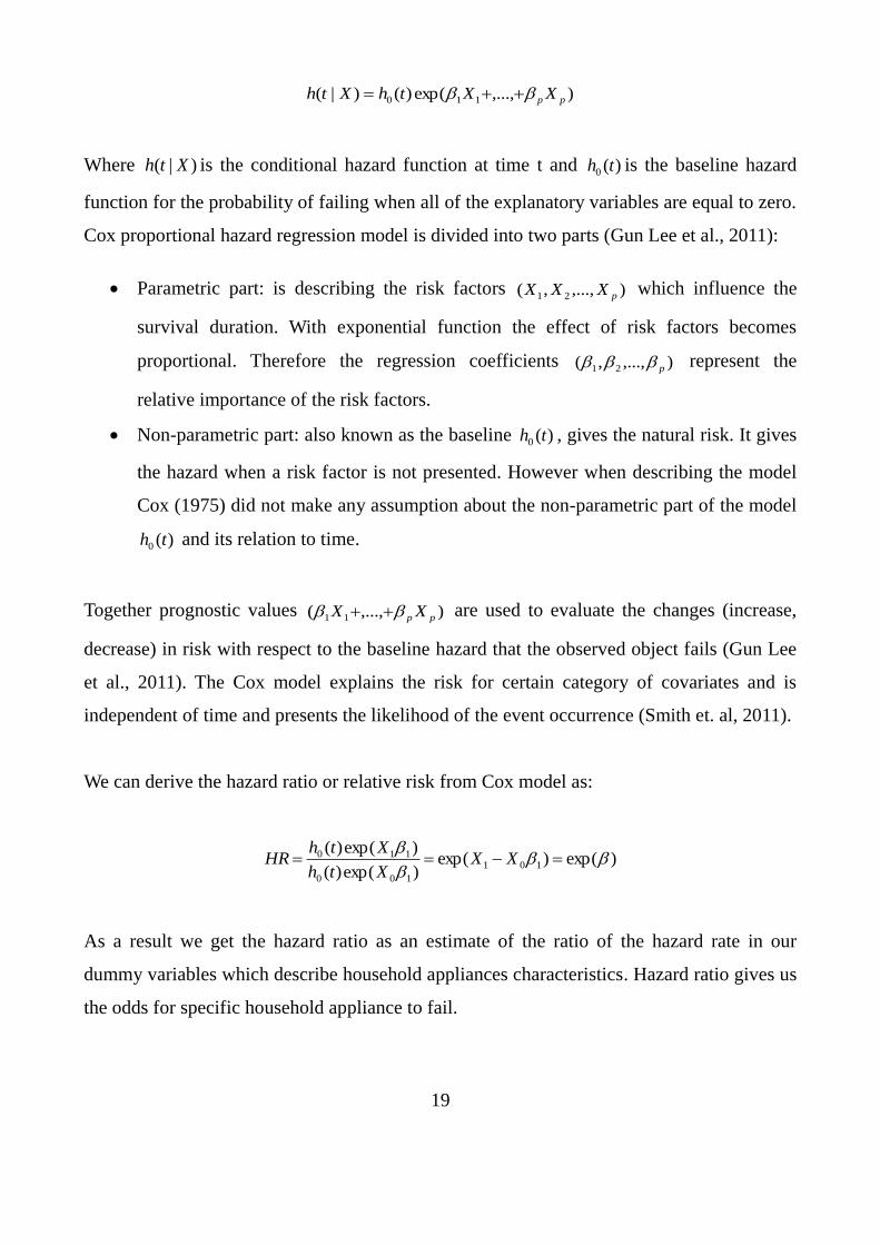
We can derive the hazard ratio or relative risk from Cox model as:
)exp()exp()exp()(
)exp()(101
100
110
XX
Xth
XthHR
As a result we get the hazard ratio as an estimate of the ratio of the hazard rate in our
dummy variables which describe household appliances characteristics. Hazard ratio gives us
the odds for specific household appliance to fail.
20
3.2 Reliability analysis for multiple failures
Our data consists of a significant amount of recurrent events which means that many
failures of household appliances appear more than once. Therefore we find it useful to
model multiple failures since it contributes to the field of product reliability. By that we also
consider the additional information of multiple failures that the single failure model does
not take into account.
There are a couple of possible models that can handle multiple failures data:
Marginal Cox model also known as WLW model (Wei et al., 1989).
Intensity model which returns the probabilities for a failure at time t, given previous
failures and covariates (Andersen and Gill, 1982).
Stratified model for “gap” times between successive failures also known as PWP
model (Prentice et al., 1981).
Even though all of above specified models have their own benefits and drawbacks we will
focus on the WLW model since it is based on previously specified Cox model and therefore
consistent with our semi-parametric reliability analysis.
3.2.1 Marginal Cox model for multiple failures
This model can be used for measuring effect of covariates on the risk of multiple failures.
We have n units and each unit can potentially experience K events (Lin, 1994). This means
that each household appliance n has a potential to fail K times. It follows each interval-
specific survival process regardless the previous observable failures and it assigns K strata
to each unit n (Liu, 2011). The marginal Cox model is specified as follows:
Where ko is baseline hazard function for the kth
event, kiZ are the covariates and k is the
column vector of regression coefficients. WLW model estimates regression coefficients
21
k ,...,1 by maximizing the partial likelihoods estimates k ˆ,...,ˆ1 separately which can be
combined to derive “average effect” estimator with the smallest asymptotic variance among
all linear estimators (Liu, 2011). By that the end estimates k'
1' ˆ,...,ˆ are considered
asymptotically jointly normal with a covariance matrix that can always be estimated without
assuming a specific correlation structure (Liu, 2011). These dependencies of multiple failure
times are adjusted by the use of a robust sandwich estimate of the variance (Parpia et al.,
2013).
By applying marginal Cox model to the multiple variables a backward elimination
procedure is proposed to get the final model with only the most important variables
included. The backward elimination begins with the model containing all potential variables
X and identifies the one with the largest p-value. If the maximum p-value is greater than the
predetermined limit than the variable is dropped. The model with remaining variables X is
fitted afterwards and the process continues until no further variables X can be dropped
(Kutner et al., 2004).
3.3 Part failure analysis
3.3.1 Pareto principle
Pareto principle, also known as 20/80 rule states that for many events, roughly 80 percent of
the effects comes from 20 percent of the causes (Chen et al., 1994). The original Pareto
principle was related to the economy and its assumption that 80 percent of a country’s
wealth is owned by 20 percent of the population (Mizuno et al., 2008).
In the reliability context, the importance of a Pareto chart is that it provides a means of
easily identifying the most frequently occurring classes, which are usually the most
important and may require urgent attention (Blischke et al., 2011).
22
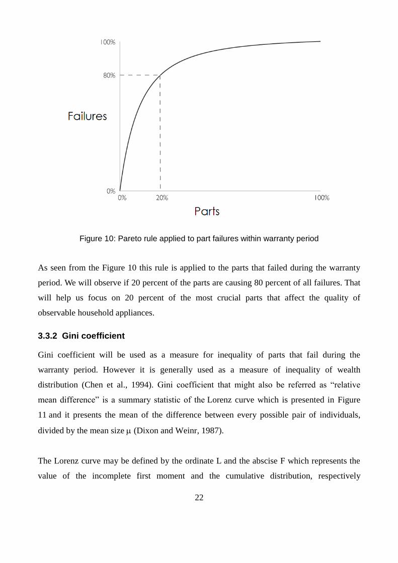
Figure 10: Pareto rule applied to part failures within warranty period
As seen from the Figure 10 this rule is applied to the parts that failed during the warranty
period. We will observe if 20 percent of the parts are causing 80 percent of all failures. That
will help us focus on 20 percent of the most crucial parts that affect the quality of
observable household appliances.
3.3.2 Gini coefficient
Gini coefficient will be used as a measure for inequality of parts that fail during the
warranty period. However it is generally used as a measure of inequality of wealth
distribution (Chen et al., 1994). Gini coefficient that might also be referred as “relative
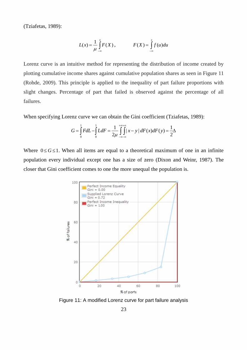
mean difference” is a summary statistic of the Lorenz curve which is presented in Figure
11 and it presents the mean of the difference between every possible pair of individuals,
divided by the mean size (Dixon and Weinr, 1987).
The Lorenz curve may be defined by the ordinate L and the abscise F which represents the
value of the incomplete first moment and the cumulative distribution, respectively
23
(Tziafetas, 1989):
x
XFxL )(1
)(
,
x
duufXF )()(
Lorenz curve is an intuitive method for representing the distribution of income created by
plotting cumulative income shares against cumulative population shares as seen in Figure 11
(Rohde, 2009). This principle is applied to the inequality of part failure proportions with
slight changes. Percentage of part that failed is observed against the percentage of all
failures.
When specifying Lorenz curve we can obtain the Gini coefficient (Tziafetas, 1989):
2
1)()(||
2
11
0
1
0
ydFxdFyxLdFFdLG
Where 10 G . When all items are equal to a theoretical maximum of one in an infinite
population every individual except one has a size of zero (Dixon and Weinr, 1987). The
closer that Gini coefficient comes to one the more unequal the population is.
Figure 11: A modified Lorenz curve for part failure analysis
24
In Figure 11 we can see visualisation of previously specified inequality measurements.
Where the 45º line presents perfect equality with a Gini coefficient equal to 0 and on the
opposite site we have 90º perfect inequality line with Gini coefficient equal to 1. In between
these two extremes we see an example of Lorenz Curve and its Gini coefficient. However
the shape of Lorenz curve might differ, depending on the data.
3.4 Warranty cost analysis
Warranty costs are inversely related to product reliability. It follows that one way of
reducing warranty costs is to improve reliability (Blischke et al., 2011). Failures and their
costs deteriorate reliability of household appliances. By definition warranty cost is the total
cost of servicing claims, considered only for the warranty period (Blischke et al., 2011).
After warranty period expires costs are not considered to be a financial burden of a company
but customer expense or distributor’s responsibility in our case.
3.4.1 Probit model
Probit regression model is used in modelling the dichotomous or binary outcome variables
(Golam Kibria and Saleh, 2012). Therefore predicting costs for different products is possible
for a probit model where we categorize our costs by:
0: not so costly failures, which are below the average costs
1: very costly failures, which are above the average costs
Probit model can be defined with latent variable y* as:
'* Xyi
We can define these binary variables as:
We can identify the relationship between binary dependent variable and other independent
25
variables as:
'
)()'(]|1Pr[
x
dttXXy , N(0,1) ~t
Where Φ is the cumulative distribution function of the standard normal distribution. By that
we are observing the probability of the outcome y=1 as a linear combination of dependent
variables. The advantage of the probit model compared to an ordinary regression model is
that predicted probabilities are limited between 0 and 1.
Marginal effects give us the difference in magnitude for the probit model coefficients and
are therefore an extension of that model. By applying marginal effects to probit model we
get the reflection of changes in probability when y=1.
jj XxP )'(
Where marginal effect includes X’s and the signs are obtained from the coefficientsj . We
can estimate marginal effects at the average of the individual marginal effects:
jjn
XxP
)'(/
Since our independent variables are all dummy variables we will use this marginal effects
and compare it to the dummy variables base line (x=0).
4 Results
4.1 Reliability analysis for a single failure
Single failure analysis was done on warranty claims data and supplementary total
production data combined. Only first failures of household appliances are considered in this
part. We include all household appliances that failed at least once within the warranty period
and compare it to the total production of household appliances that did not fail.
4.1.1 Testing proportional hazard assumptions
Before proceeding with Cox PH model we need to test proportional hazard assumption for
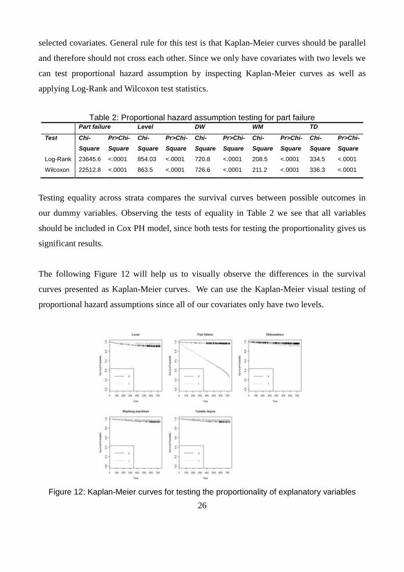
26
selected covariates. General rule for this test is that Kaplan-Meier curves should be parallel
and therefore should not cross each other. Since we only have covariates with two levels we
can test proportional hazard assumption by inspecting Kaplan-Meier curves as well as
applying Log-Rank and Wilcoxon test statistics.
Table 2: Proportional hazard assumption testing for part failure
Part failure Level DW WM TD
Test Chi-
Square
Pr>Chi-
Square
Chi-
Square
Pr>Chi-
Square
Chi-
Square
Pr>Chi-
Square
Chi-
Square
Pr>Chi-
Square
Chi-
Square
Pr>Chi-
Square
Log-Rank 23645.6 <.0001 854.03 <.0001 720.8 <.0001 208.5 <.0001 334.5 <.0001
Wilcoxon 22512.8 <.0001 863.5 <.0001 726.6 <.0001 211.2 <.0001 336.3 <.0001
Testing equality across strata compares the survival curves between possible outcomes in
our dummy variables. Observing the tests of equality in Table 2 we see that all variables
should be included in Cox PH model, since both tests for testing the proportionality gives us
significant results.
The following Figure 12 will help us to visually observe the differences in the survival
curves presented as Kaplan-Meier curves. We can use the Kaplan-Meier visual testing of
proportional hazard assumptions since all of our covariates only have two levels.
Figure 12: Kaplan-Meier curves for testing the proportionality of explanatory variables
27
Figure 12 shows parallel curves for each of the covariates. They do not cross each other
which is an indication that the survival curves do not violate proportional hazard
assumption. From Figure 12 it is obvious that there are big differences between household
appliances with no or minor failure and part failures that need replacement.
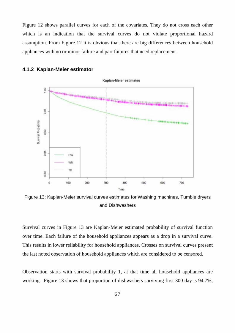
4.1.2 Kaplan-Meier estimator
Figure 13: Kaplan-Meier survival curves estimates for Washing machines, Tumble dryers
and Dishwashers
Survival curves in Figure 13 are Kaplan-Meier estimated probability of survival function
over time. Each failure of the household appliances appears as a drop in a survival curve.
This results in lower reliability for household appliances. Crosses on survival curves present
the last noted observation of household appliances which are considered to be censored.
Observation starts with survival probability 1, at that time all household appliances are
working. Figure 13 shows that proportion of dishwashers surviving first 300 day is 94.7%,
28
representing the lowest reliability among all household appliances. On the other hand
proportion of tumble dryers surviving first 300 days is the highest and is 97.8%. Proportion
of washing machines that surviving first 300 days is 98.2%. We see that after 300 day of
household appliances usage the survival curve becomes almost horizontal because the
number of failures drops significantly. Our last observable time that is not censored is day
730 which is the last day before warranty expires. The final survival probability reaches
90.9% for dishwashers, 95.4% for washing machines and 96.2% for tumble dryers.
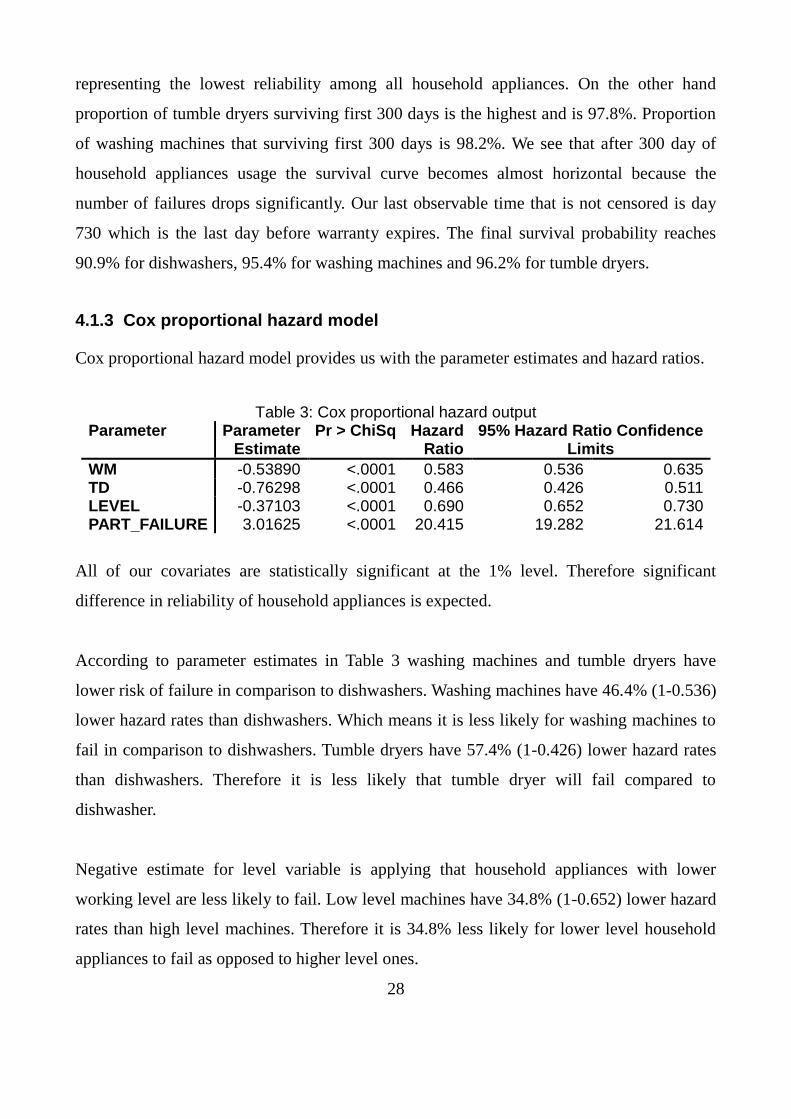
4.1.3 Cox proportional hazard model
Cox proportional hazard model provides us with the parameter estimates and hazard ratios.
Table 3: Cox proportional hazard output Parameter Parameter
Estimate Pr > ChiSq Hazard
Ratio 95% Hazard Ratio Confidence
Limits
WM -0.53890 <.0001 0.583 0.536 0.635 TD -0.76298 <.0001 0.466 0.426 0.511 LEVEL -0.37103 <.0001 0.690 0.652 0.730 PART_FAILURE 3.01625 <.0001 20.415 19.282 21.614
All of our covariates are statistically significant at the 1% level. Therefore significant
difference in reliability of household appliances is expected.
According to parameter estimates in Table 3 washing machines and tumble dryers have
lower risk of failure in comparison to dishwashers. Washing machines have 46.4% (1-0.536)
lower hazard rates than dishwashers. Which means it is less likely for washing machines to
fail in comparison to dishwashers. Tumble dryers have 57.4% (1-0.426) lower hazard rates
than dishwashers. Therefore it is less likely that tumble dryer will fail compared to
dishwasher.
Negative estimate for level variable is applying that household appliances with lower
working level are less likely to fail. Low level machines have 34.8% (1-0.652) lower hazard
rates than high level machines. Therefore it is 34.8% less likely for lower level household
appliances to fail as opposed to higher level ones.
29
Household appliances with a noted part failure that needed replacement are more likely to
fail. The hazard ratio for this variable is really large (19.282). Hence the household
appliances with part failure that needed replacement are 19 times more likely to fail than
those without the failure or a minor failure.
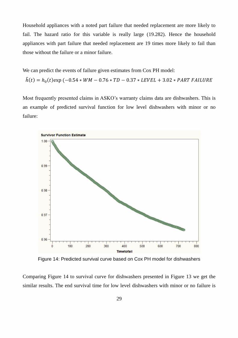
We can predict the events of failure given estimates from Cox PH model:
Most frequently presented claims in ASKO’s warranty claims data are dishwashers. This is
an example of predicted survival function for low level dishwashers with minor or no
failure:
Figure 14: Predicted survival curve based on Cox PH model for dishwashers
Comparing Figure 14 to survival curve for dishwashers presented in Figure 13 we get the
similar results. The end survival time for low level dishwashers with minor or no failure is
30
around 96%. This ending survival probability is a little higher comparing to the Kaplan-
Meier survival curve in Figure 13 due to the fact that dishwashers with part failure are not
considered in this prediction.
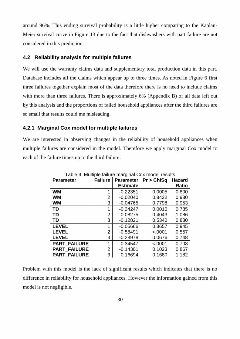
4.2 Reliability analysis for multiple failures
We will use the warranty claims data and supplementary total production data in this part.
Database includes all the claims which appear up to three times. As noted in Figure 6 first
three failures together explain most of the data therefore there is no need to include claims
with more than three failures. There is approximately 6% (Appendix B) of all data left out
by this analysis and the proportions of failed household appliances after the third failures are
so small that results could me misleading.
4.2.1 Marginal Cox model for multiple failures
We are interested in observing changes in the reliability of household appliances when
multiple failures are considered in the model. Therefore we apply marginal Cox model to
each of the failure times up to the third failure.
Table 4: Multiple failure marginal Cox model results Parameter Failure Parameter
Estimate Pr > ChiSq Hazard
Ratio
WM 1 -0.22351 0.0005 0.800 WM 2 -0.02040 0.8422 0.980 WM 3 -0.04765 0.7798 0.953
TD 1 -0.24247 0.0010 0.785 TD 2 0.08275 0.4043 1.086 TD 3 -0.12821 0.5340 0.880
LEVEL 1 -0.05666 0.3657 0.945 LEVEL 2 -0.58491 <.0001 0.557 LEVEL 3 -0.28978 0.0676 0.748
PART_FAILURE 1 -0.34547 <.0001 0.708 PART_FAILURE 2 -0.14301 0.1023 0.867 PART_FAILURE 3 0.16694 0.1680 1.182
Problem with this model is the lack of significant results which indicates that there is no
difference in reliability for household appliances. However the information gained from this
model is not negligible.
31
Similar as in Table 3, Table 4 shows that washing machines have lower risk of failure than
dishwashers regardless the number of failures. We can also see from the Table 4 that hazard
rates decreases with each additional failure. Washing machines with three failures have 5%
(1-0.953) lower hazard rates than dishwashers while washing machines with one failure
have 20% (1-0.8) lower hazard rates in comparison to dishwashers. Second and third
failures are highly insignificant and these results are therefore not so accurate.
We get similar results for tumble dryers but with one change for the second failure. Table 4
shows there is higher likelihood of failure for tumble dryers as oppose to dishwashers.
Hence tumble dryers with two failures are 1.086 times more likely to fail than dishwashers
with the same amount of failures. As before changes in reliability are not significant.
Lower level household appliances are less likely to fail than high level ones regardless the
number of failures. At the 10% significant level we can conclude that low household
appliances with two failures are 45% (1-0,557) less likely to fail than high level household
appliances. This risk decreases for 18% with an additional third failure.
Household appliances with part failure that needed replacement are less likely to fail one or
two times. These results are slightly different than for singular failure Cox PH model in
Table 3, where part failure is associated with much higher likelihood of household
appliances failure.
Even though marginal Cox model is in some way informative there is a big chance of
randomness presented in the results. For the further investigation of given results we run a
backward elimination to select the most important variables for this model.
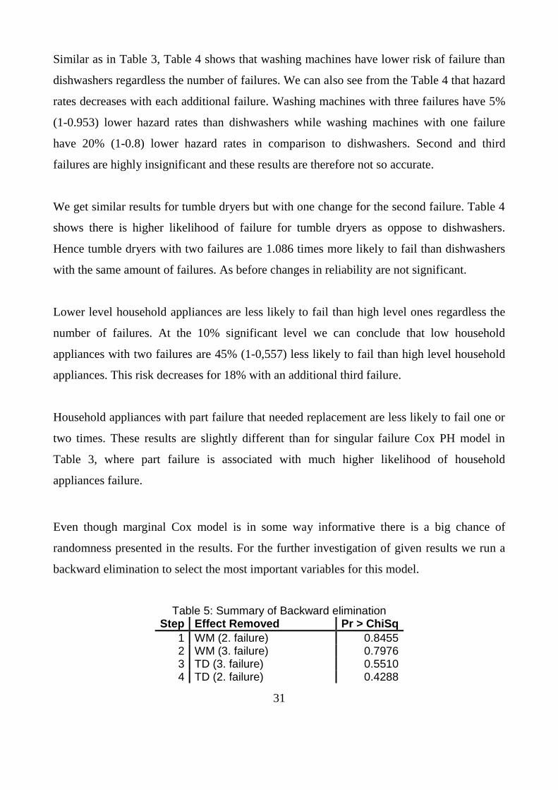
Table 5: Summary of Backward elimination Step Effect Removed Pr > ChiSq
1 WM (2. failure) 0.8455 2 WM (3. failure) 0.7976 3 TD (3. failure) 0.5510 4 TD (2. failure) 0.4288
32
5 PART FAILURE (3. failure) 0.2653
We can see from the Table 5 that only second and third failure variables are eliminated from
the model. Observing all of the covariates we can exclude information about the third
failure for all of them except the level. These results are obtained when the level of
significance is specified at 7%.
Table 6: Multiple failure marginal Cox model results after the backward elimination Parameter Failure Parameter
Estimate Pr > ChiSq Hazard
Ratio
WM 1 -0.22351 <.0001 0.800
TD 1 -0.24247 <.0001 0.785
LEVEL 1 -0.05666 0.0423 0.945 LEVEL 2 -0.58060 <.0001 0.560 LEVEL 3 -0.28568 0.0645 0.752
PART FAILURE 1 -0.34547 <.0001 0.708 PART FAILURE 2 -0.13580 0.0667 0.873
With backward elimination we get all the significant (7% significance level) variables
included in the model. As seen in Table 6 all of the first failure covariates are still included
in the model. With marginal Cox model we can still observe the changes in hazard ratio for
level variable for all three failures. The hazard ratio changes slightly for variables with
multiple failures that are still presented in the final model. The risk of failure increases for
38% from the first to second failure (44%-6%) when comparing the low level and the high
level household appliances. There is also higher risk for the third failure comparing to the
first failure for low level household appliances than the high level household appliances.
The risk of failure decreases for household appliances with part failure after the first failure.
Table 7: Model Fit Statistics First failure Multiple failure
Criterion Without Covariates
With Covariates
Without Covariates
With Covariates
-2 LOG L 118041.41 108580.24 104325.01 104024.92 AIC 118041.41 108588.24 104325.01 104048.92
33
Evaluating the fit for first failure model and the final multiple failures modal after backward
elimination, model fit statistics indicates that multiple failure model is better but only
slightly.
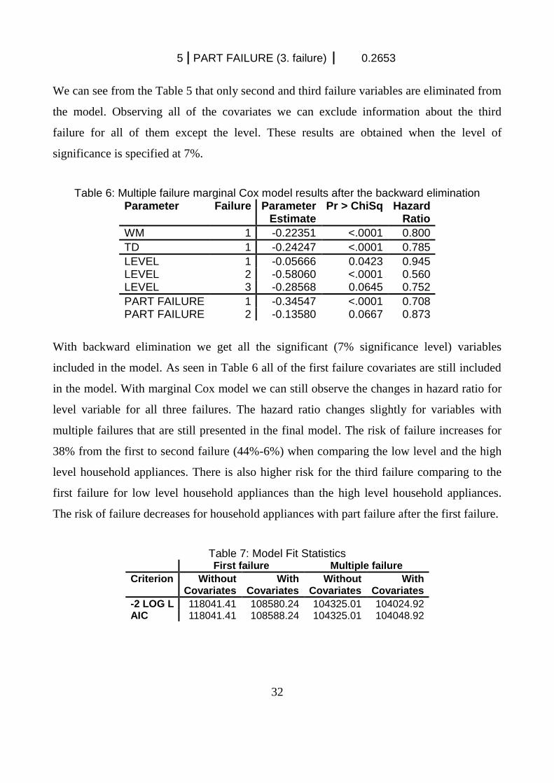
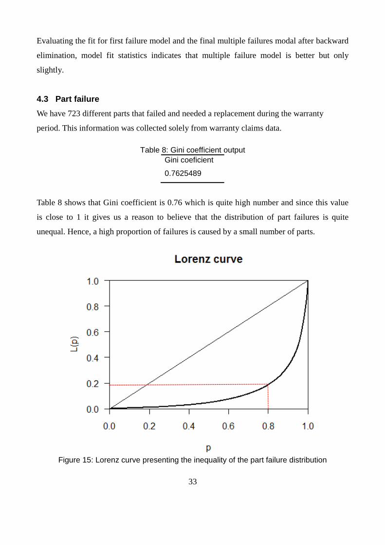
4.3 Part failure
We have 723 different parts that failed and needed a replacement during the warranty
period. This information was collected solely from warranty claims data.
Table 8: Gini coefficient output
Gini coeficient
0.7625489
Table 8 shows that Gini coefficient is 0.76 which is quite high number and since this value
is close to 1 it gives us a reason to believe that the distribution of part failures is quite
unequal. Hence, a high proportion of failures is caused by a small number of parts.
Figure 15: Lorenz curve presenting the inequality of the part failure distribution
34
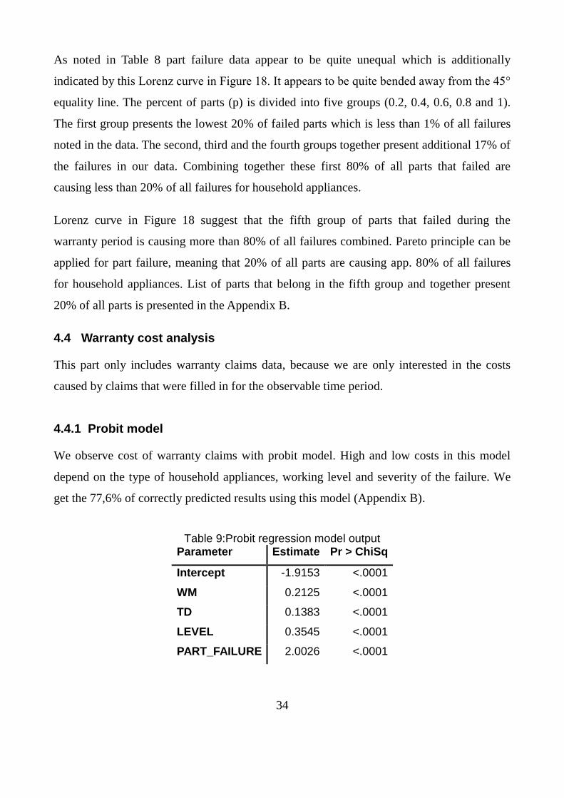
As noted in Table 8 part failure data appear to be quite unequal which is additionally
indicated by this Lorenz curve in Figure 18. It appears to be quite bended away from the 45°
equality line. The percent of parts (p) is divided into five groups (0.2, 0.4, 0.6, 0.8 and 1).
The first group presents the lowest 20% of failed parts which is less than 1% of all failures
noted in the data. The second, third and the fourth groups together present additional 17% of
the failures in our data. Combining together these first 80% of all parts that failed are
causing less than 20% of all failures for household appliances.
Lorenz curve in Figure 18 suggest that the fifth group of parts that failed during the
warranty period is causing more than 80% of all failures combined. Pareto principle can be
applied for part failure, meaning that 20% of all parts are causing app. 80% of all failures
for household appliances. List of parts that belong in the fifth group and together present
20% of all parts is presented in the Appendix B.
4.4 Warranty cost analysis
This part only includes warranty claims data, because we are only interested in the costs
caused by claims that were filled in for the observable time period.
4.4.1 Probit model
We observe cost of warranty claims with probit model. High and low costs in this model
depend on the type of household appliances, working level and severity of the failure. We
get the 77,6% of correctly predicted results using this model (Appendix B).
Table 9:Probit regression model output Parameter Estimate Pr > ChiSq
Intercept -1.9153 <.0001
WM 0.2125 <.0001
TD 0.1383 <.0001
LEVEL 0.3545 <.0001
PART_FAILURE 2.0026 <.0001
35
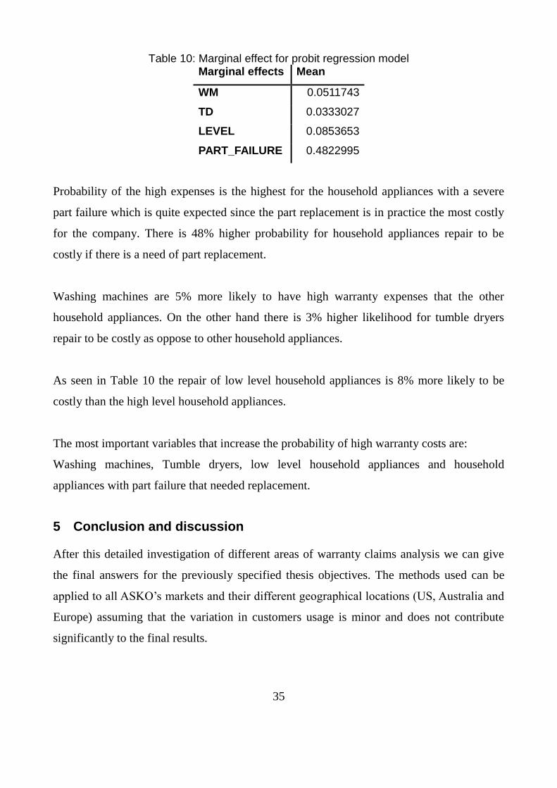
Table 10: Marginal effect for probit regression model Marginal effects Mean
WM 0.0511743
TD 0.0333027
LEVEL 0.0853653
PART_FAILURE 0.4822995
Probability of the high expenses is the highest for the household appliances with a severe
part failure which is quite expected since the part replacement is in practice the most costly
for the company. There is 48% higher probability for household appliances repair to be
costly if there is a need of part replacement.
Washing machines are 5% more likely to have high warranty expenses that the other
household appliances. On the other hand there is 3% higher likelihood for tumble dryers
repair to be costly as oppose to other household appliances.
As seen in Table 10 the repair of low level household appliances is 8% more likely to be
costly than the high level household appliances.
The most important variables that increase the probability of high warranty costs are:
Washing machines, Tumble dryers, low level household appliances and household
appliances with part failure that needed replacement.
5 Conclusion and discussion
After this detailed investigation of different areas of warranty claims analysis we can give
the final answers for the previously specified thesis objectives. The methods used can be
applied to all ASKO’s markets and their different geographical locations (US, Australia and
Europe) assuming that the variation in customers usage is minor and does not contribute
significantly to the final results.
36
Estimate the probability of product failure within 2 years warranty period for each
household appliance to get a better overview of the warranty period.
Both non-parametric and semi-parametric methods for reliability analysis gave us similar
results when it comes to predicting the household appliances reliability. As noted, the
probability of product failure decreases steadily throughout household appliances lifetime in
the warranty period. Moreover the life time of observable household appliances follows the
right skewed distribution (Figure 3, Figure 4 and Figure 5) and therefore it seems that the
first months are the most critical for reliability of household appliances. Mass of failures is
concentrated in the beginning of household appliances life circle hence the probability for
the failure to occur is decreasing with time. Kaplan-Meier estimates in Figure 13 shows that
more than 90% of all household appliances survive the first two years. Moreover there are
not many failures noted after the first year of usage. Therefore the survival curve becomes
almost horizontal. This gives us a reason to believe that a longer warranty period is
reasonable for ASKO but since we did not focus on the whole life cycle of household
appliances some caution is advisable. The problem arises with a certain point in the lifetime
of household appliances when mass failure is expected and because we did not reach that
point with our analysis it is hard to predict it. The bathtub curve can describe such
behaviour. The last so called wear out part in the bathtub curve was not taken into
consideration in this thesis. To get the full overview of household appliances reliability we
would need to observe their whole lifetime, not only the warranty period.
According to different methods (Kapla-Meier estimates, Cox proportional hazard analysis)
that were used in this thesis, the highest risk for failure among household appliances was
observed for dishwashers. Overall there is a high risk of failure for household appliances
that experienced part failure and are known to be high level products. These factors mostly
influence reliability of the observed household appliances.
Identify the most frequent warranty events (failures) to discover the most unreliable
parts that influence the proper functioning of the household appliances.
37
Our second objective focuses on parts that failed within warranty period and needed
replacement. We discovered that this problem follows Pareto rule, meaning that 20%
(presented in Appendix B) of parts that fail cause 80% of all failures. Such an inequality in
data is in some sense quite useful because it is easier to identify the main cause of the
failures since the probability that one of the 20% most frequently noted failed parts will
appear is quite high. However this information also gives us a reason to assume some
serious quality problems with most frequently failed parts. Especially the first 10 most
frequently presented part failures that are presented in Figure 9 would need additional
quality control analysis to indentify the core cause of these frequent failures.
Estimate warranty expenses for different products regarding the repair and labour
costs.
By applying the probit model to warranty costs data we get the valuable information about
the influence of specific characteristics of household appliances for the high costs. We see
that there is a high probability of high costs for household appliances with part failure.
Linking that result with the information from Cox PH model in Table 3, it can be shown that
part failure is not only more likely to be financial burden for ASKO but is also highly likely
to occur in the warranty period. Moreover the quality control analysis that was investigated
as a second objective might be helpful in dealing with this problem since it narrows the
causes (possible part failures) for high costs.
Other three covariates imply higher costs for washing machines, tumble dryers and low
level household appliances. Knowing that these household appliances are less likely to fail
from the Cox PH model in Table 3 is quite beneficial for ASKO since household appliances
that tend to have lower risk of failure are more likely to be less costly.
Methods
Both semi-parametric and non-parametric approaches were used for reliability analyses.
There is not a big difference in results when applying these two methods. On one hand, non-
38
parametric Kaplan-Meier estimator is a simple way to predict survival curve for household
appliances but the simplicity is also its downside because it lacks in flexibility. Moreover it
can include the censoring information which is very important for the reliability analysis
and its visualisation of survival courses stratified by groups of household appliances is quite
informative. On the other hand, all of the deficits from Kaplan-Meier estimator can be
repaired by applying Cox PH model. Its flexibility gives it the ability to implement
characteristics of household appliances in the results. Moreover given estimates can be
further used for the prediction of survival curve where specific characteristic can be plugged
in the model. Additionally hazard ratio is a useful way to predict the risk of failure and set a
value which might sometimes be more informative than the visualisation.
There was an attempt for prediction of future failures from household appliances with Box-
Jenkins ARIMA model (Appendix B) that were just informational and are therefore not
included in this result part of the thesis. In the research work of Ho and Xie (1998) we see
that ARIMA models are very flexible and have quite satisfactory predictive performance for
analyzing the failure data. However the results presented in Appendix B show really wide
confidence intervals for the future events therefore the information gained from the ARIMA
model is not so valuable.
When comparing result between single failure Cox PH model and multiple failures marginal
Cox model we see that instead of including most of the data or information in the model, we
should rather focus on the quality of the results. More reliable results are presented in the
single failure model. Even though this means that some information is omitted, all
household appliances are included in the model but without the additional failures. However
after proceeding with backward elimination only the most important variables are included
in the marginal Cox model and this is the way to improve the initial results.
Since this thesis focuses mostly on likelihood of event to happen (both non-parametric and
parametric models) the reasonable way to model warranty costs was with a usage of probit
39
model. It is beneficial to be able to compare results from reliability analysis with cost
analysis and therefore the 0 to 1 range when predicting the costs is a big advantage.
Relationship between dependent variable which is then total number of costs and several
independent variables that are describing characteristics of household appliances is possible
to analyse with simple multiple linear regression model. The results are presented in
Appendix B. However interpretation of the result for multiple linear regressions is not as
informative as when using probit model since it is not reasonable to get the exact value of
costs per household appliances.
6 Future work
The important issue emerged from a specification of censored data. Additional information
and with that improvement of the model could be gained from specification of the period
from the last failure of the household appliances to the end of warranty period. To date no
known research work has reported how to handle this issue. A proposal to approach this
issue is to include the time period from the last failure to the end of the warranty period as a
new reported claim in the warranty claims database. This additional information should be
censored after the last day of warranty period.
Even though we got some basic information about the most frequent part failures additional
quality analysis is recommended to get a deeper understanding to the problem. This
concerns especially those 20% failures that appear most frequently. Further analysis of most
frequent part failures would be recommended for the purpose of part quality assessment.
One way to approach this problem is with a Ishikawa diagrams (also known as fishbone
diagrams) where the factors causing the frequent failures can be identified.
Only one market (US) was observed in this thesis therefore a future comparison between
different markets would be advisable. Significant changes in results for different markets
may draw the attention on potential problems.
40
When observing Figure 7 which presents the number of extreme failures per household
appliances, we discovered that most of the failures are caused by household appliances
produced a year or two before the actual purchase. Therefore considering the time from
production to the purchase in future studies would be advisable. This is so called leverage
time and is a part of earlier mentioned reliability at sale analysis.
41
7 Literature
Amato H. N., E. L. Anderson and D. W. Harvey. (1976). A General Model of Future
PeriodWarranty Costs. The Accounting Review, 1(4).
Andersen P. K. and R. D. Gill. (1982). Cox’s Regression Model Counting Process: A Large
Sample Study. Annals of Statistics, 10: 1100–20.
Blischke, W. R., and D. N. P. Murthy. (1994). Warranty Cost Analysis. New York: M.
Dekker.
Chukova, S., and Yu Hayakawa. (2004). Warranty Cost Analysis: Non-zero Repair Time.
Applied Stochastic Models in Business and Industry, 20(1): 59-71.
Cox D. R. (1972). Regression Models and Life-Tables. Journal of the Royal Statistical
Society, 34(2): 187-220. Accessed April, 2013 on website: http://links.jstor.org/
Dixon P. M., J. Weiner, T. Mitchell-Olds and R. Woodley. (1987). Bootstrapping the Gini
Coefficient of Inequality. Ecology, 68: 1548-51.
E. L. Kaplan and P. Meier Source. (1958). Nonparametric Estimation from Incomplete
Observations. Journal of the American Statistical Association, 282(53): 457- 81. Accessed
March, 2013 on website: http://www.jstor.org/stable/2281868 Accessed: 16/01/2009 11:28
Golam Kibria B.M. and A.K.Md.E. Saleh (2012). Improving the estimators of the
parameters of a probit regression model: A ridge regression approach. Journal of Statistical
Planning and Inference, 142(6): 1421-35.
Gun Lee J., S. Moon and K. Salamatian (2012) Modeling and predicting the popularity of
online contents with Cox proportional hazard regression model. Neurocomputing, 76(1):
134-45. Accessed April, 2013 on website:http://ac.els-cdn.com/S0925231211004218/1-s2.0-
S0925231211004218-main.pdf?_tid=dacd56e6-b639-11e2-a321-
00000aab0f02&acdnat=1367837217_24abc3b3a83aefa8f7d985919b671774
Hagen J., Adams T., Potts R., Hammarstrom K., Dietzman R., BeckerJ., Froning D. and
Johnson J. (2013). Warranty best practices and process improvements. Accessed February,
42
2013 on webpage: https://www.warrantyvideo.com/index.php?option=com_content&view=
article&id=202:warranty-best-practices-a-process-improvements-
video&catid=903&Itemid=7
Heitjan D.F. and Rubin D.B. (1991). Ignorability and coarse data. Annals of Statistics,
19(4): 2244–53. Accessed March, 2013 on website: http://projecteuclid.org/DPubS?service=
Ho S.L., and M. Xie. (1998). The Use of ARIMA Models for Reliability Forecasting and
Analysis. Computers & Industrial Engineering, 35(1-2): 213-16.
Kleinbaum D.G, and M. Klein. (2012). Survival Analysis- A Self-Learning Text, Second
Edition. Springer: New York.
Kotler, P. (1976). Marketing Management-Analysis, Prentice-Hall, Englewood Cliffs, NJ.
Kulkarni V., and S. I. Resnick. (2008). Warranty Claims Modeling. Naval Research
Logistics 55(4): 339-49.
Kutner, Michael H., Christopher J. Nachtsheim, John Neter, and William Li. Applied Linear
Statistical Models. 5th ed. Boston: McGraw-Hill Irwin, 2004.
Lin D. Y. (1994) Cox Regression Analysis of Multivariate Failure Time Data: The Marginal
Approach. Statistics in Medicine, 13: 2233–47.
Liu, X. (2012). Survival Analysis: Models and Applications. Chichester, West Sussex:
Wiley/Higher Education.
Murthy, D.N.P., and I. Djamaludin. (2002). New Product Warranty: A Literature Review.
International journal of production economics, 79(3): 231-60. Accessed February, 2013 on
webpage: http://www.alvarestech.com/temp/PDP2011/emc6605.ogliari.prof.ufsc.br/
Patankar, J.G. and Mitra, A. (1995). Effect of warranty execution on warranty reserve costs.
Management Science, 41(3): 395–400.
Percy D. (2002). Bayesian Enhanced Strategic Decision Making for Reliability. European
Journal of Operational Research, 139:133-45.
43
Prentice R. L., B. J. Williams and A. V. Peterson. (1981). On the Regression Analysis of
Multivariate Failure Time Data. Biometrika, 68: 373–9.
Restrito/New%20product%20warranty_%20a%20literature%20review.pdf
Rohde N. (2009). An alternative functional form for estimating the Lorenz curve.
Economics Letters, 105(1): 61-3.
Sameer P., L. Thabane, J. A Julian, T. J Whelan and M. N Levine (2013). Empirical
comparison of methods for analyzing multiple time-to-event outcomes in anon-inferiority
trial: a breast cancer study. BMC Medical Research Methodology, 13: 44. Accessed May,
2013 on website: http://www.biomedcentral.com/1471-2288/13/44#B19sici?sici=0035-
9246%281972%2934%3A2%3C187%3ARMAL%3E2.0.CO%3B2-6
Smith T. and B. Smith. (2004). Kaplan Meier and Cox Proportional Hazard Modelling:
Hands on Survival Analysis. WUSS. Accessed April, 2013 on website:
http://www.lexjansen.com/wuss/2004/hands_on_workshops/i_how_kaplan_meier_and_cox
_p.pdf
Smith T., Smith B and M. AK Ryan. (2011). Survival Analysis Using Cox Proportional
Hazards Modeling For Single And Multiple Event Time Data. Accessed April, 2013 on
website: http://medicine.yale.edu/labs/ma/www/BIS643/254-28.pdf
Spruance S. L., J. E. Reid, M. Grace and M. Samore. (2004). Hazard Ratio in Clinical
Trials. Antimicrob Agents Chemother, 48(8): 2787–92. Accessed April, 2013 on website:
Steinberg, W. J. (2011). Statistics alive! Thousand Oaks, CA: Sage Publications.
Takayuki M., M. Toriyama, T. Terano, M. Takayasu. (2008). Pareto law of the expenditure
of a person in convenience store. Statistical Mechanic and its Applications, 387(15): 3931-
35.
Twisk, J., N. Smidt, and W. De Vente. (2005). Applied Analysis of Recurrent Events: A
Practical Overview. Journal of Epidemiology Community Health, 59(9): 706-10. Accessed
44
May, 2013 on website: <http://www.ncbi.nlm.nih.gov/pmc/articles/PMC1733116/>.
Tziafetas B. J. (1989). A Formula for the Gini Coefficient and its Decomposition.
Biometrical Journal, 31(8):961-7. Accessed May, 2013 on website: http://onlinelibrary.
wiley.com.lt.ltag.bibl.liu.se/doi/10.1002/bimj.4710310811/pdf =
ucla.edu. (2013). Survival Analysis with SAS. UCLA: Statistical Consulting Group.
Accessed March, 2013 on website: http://www.ats.ucla.edu/stat/sas/seminars/sas_survival/
UI&version=1.0&verb=Display&handle=euclid.aos/1176348396
V. González Díaz, J.F. Gómez, M. López, A. Crespo and P. Moreu de León. (2009).
Warranty cost models State-of-Art: A practical review to the framework of warranty cost
management. ESREL 2009, Prague. Accessed February, 2013 on webpage:
http://taylor.us.es/sim/documentos/resultados/ESREL_09_warranty_VGD.pdf
Wei L. J., D. Y. Lin and L. Weissfeld . (1989). Regression Analysis of Multivariate
Incomplete Failure Time Data by Modeling Marginal Distribution. Journal of the American
Statistical Association, 84: 1065–73.
Wu S. (2013). A review on coarse warranty data and analysis. Reliability Engineering &
System Safety. 114: 1–11.
Wu, S. (2010). Warranty claim analysis considering human factors. Reliability Engineering
and System Safety 96(1): 131-38. Accessed May, 2013 on website:
https://dspace.lib.cranfield.ac.uk/bitstream/1826/4729/4/Warranty_claim_analysis-2011.pdf
Y.-S. Chen, P.P. Chong and M.Y. Tong. (1994). Mathematical and computer modelling of
the Pareto principle. Mathematical and Computer Modelling, 19(9): 61-80.
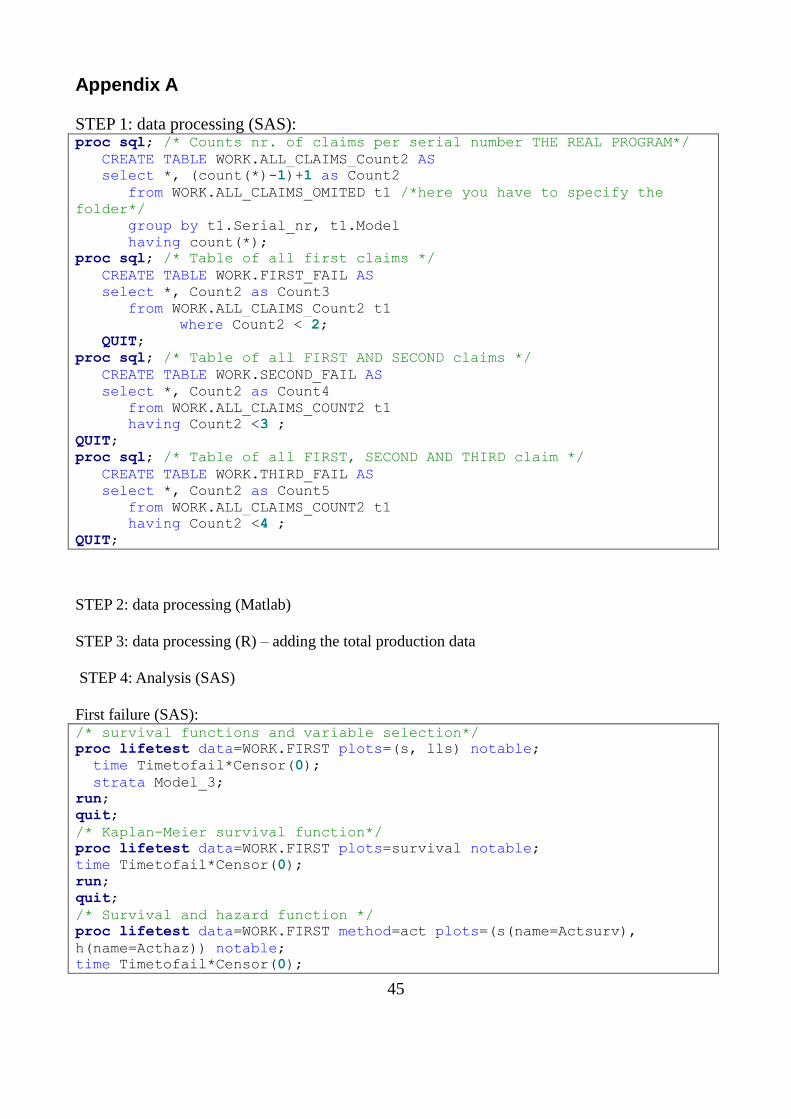
45
Appendix A
STEP 1: data processing (SAS): proc sql; /* Counts nr. of claims per serial number THE REAL PROGRAM*/
CREATE TABLE WORK.ALL_CLAIMS_Count2 AS
select *, (count(*)-1)+1 as Count2
from WORK.ALL_CLAIMS_OMITED t1 /*here you have to specify the
folder*/
group by t1.Serial_nr, t1.Model
having count(*);
proc sql; /* Table of all first claims */
CREATE TABLE WORK.FIRST_FAIL AS
select *, Count2 as Count3
from WORK.ALL_CLAIMS_Count2 t1
where Count2 < 2;
QUIT;
proc sql; /* Table of all FIRST AND SECOND claims */
CREATE TABLE WORK.SECOND_FAIL AS
select *, Count2 as Count4
from WORK.ALL_CLAIMS_COUNT2 t1
having Count2 <3 ;
QUIT;
proc sql; /* Table of all FIRST, SECOND AND THIRD claim */
CREATE TABLE WORK.THIRD_FAIL AS
select *, Count2 as Count5
from WORK.ALL_CLAIMS_COUNT2 t1
having Count2 <4 ;
QUIT;
STEP 2: data processing (Matlab)
STEP 3: data processing (R) – adding the total production data
STEP 4: Analysis (SAS)
First failure (SAS): /* survival functions and variable selection*/
proc lifetest data=WORK.FIRST plots=(s, lls) notable;
time Timetofail*Censor(0);
strata Model_3;
run;
quit;
/* Kaplan-Meier survival function*/
proc lifetest data=WORK.FIRST plots=survival notable;
time Timetofail*Censor(0);
run;
quit;
/* Survival and hazard function */
proc lifetest data=WORK.FIRST method=act plots=(s(name=Actsurv),
h(name=Acthaz)) notable;
time Timetofail*Censor(0);
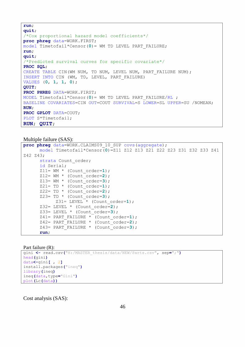
46
run;
quit;
/*Cox proportional hazard model coefficients*/
proc phreg data=WORK.FIRST;
model Timetofail*Censor(0)= WM TD LEVEL PART_FAILURE;
run;
quit;
/*Predicted survival curves for specific covariate*/
PROC SQL;
CREATE TABLE CIN(WM NUM, TD NUM, LEVEL NUM, PART_FAILURE NUM);
INSERT INTO CIN (WM, TD, LEVEL, PART_FAILURE)
VALUES (0, 1, 1, 0);
QUIT;
PROC PHREG DATA=WORK.FIRST;
MODEL Timetofail*Censor(0)= WM TD LEVEL PART_FAILURE/RL ;
BASELINE COVARIATES=CIN OUT=COUT SURVIVAL=S LOWER=SL UPPER=SU /NOMEAN;
RUN;
PROC GPLOT DATA=COUT;
PLOT S*Timetofail;
RUN; QUIT;
Multiple failure (SAS): proc phreg data=WORK.CLAIMS09_10_SUP covs(aggregate);
model Timetofail*Censor(0)=Z11 Z12 Z13 Z21 Z22 Z23 Z31 Z32 Z33 Z41
Z42 Z43;
strata Count_order;
id Serial;
Z11= WM * (Count_order=1);
Z12= WM * (Count_order=2);
Z13= WM * (Count_order=3);
Z21= TD * (Count_order=1);
Z22= TD * (Count_order=2);
Z23= TD * (Count_order=3);
Z31= LEVEL * (Count_order=1);
Z32= LEVEL * (Count_order=2);
Z33= LEVEL * (Count_order=3);
Z41= PART_FAILURE * (Count_order=1);
Z42= PART_FAILURE * (Count_order=2);
Z43= PART_FAILURE * (Count_order=3);
run;
Part failure (R): gini <- read.csv("H:/MASTER_thesis/data/NEW/Parts.csv", sep=";")
head(gini)
data<-gini[ , 2]
install.packages("ineq")
library(ineq)
ineq(data,type="Gini")
plot(Lc(data))
Cost analysis (SAS):
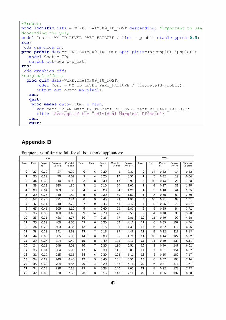
47
*Probit;
proc logistic data = WORK.CLAIMS09_10_COST descending; *important to use
descending for y=1;
model Cost = WM TD LEVEL PART_FAILURE / link = probit ctable pprob=0.5;
run;
ods graphics on;
proc probit data=WORK.CLAIMS09_10_COST optc plots=(predpplot ippplot);
model Cost = TD;
output out=new p=p_hat;
run;
ods graphics off;
*marginal effect;
proc qlim data=WORK.CLAIMS09_10_COST;
model Cost = WM TD LEVEL PART_FAILURE / discrete(d=probit);
output out=outme marginal;
run;
quit;
proc means data=outme n mean;
var Meff_P2_WM Meff_P2_TD Meff_P2_LEVEL Meff_P2_PART_FAILURE;
title 'Average of the Individual Marginal Effects';
run;
quit;
Appendix B
Frequencies of time to fail for all household appliances: DW TD WM
Time Freq Percent
Cumulative freq
Cumulative perc
Time Freq Percent
Cumulative freq
Cumulative_perc
Time Freq Percent
Cumulative_fre
q
Cumulative_perc
0 37 0.32 37 0.32 0 6 0.30 6 0.30 0 14 0.62 14 0.62
1 33 0.29 70 0.61 1 4 0.20 10 0.50 1 5 0.22 19 0.84
2 44 0.38 114 0.99 2 8 0.40 18 0.90 2 10 0.44 29 1.28
3 36 0.31 150 1.30 3 2 0.10 20 1.00 3 6 0.27 35 1.55
4 39 0.34 189 1.63 4 4 0.20 24 1.20 4 9 0.40 44 1.95
5 30 0.26 219 1.89 5 6 0.30 30 1.50 5 8 0.35 52 2.30
6 52 0.45 271 2.34 6 9 0.45 39 1.95 6 16 0.71 68 3.01
7 47 0.41 318 2.75 7 9 0.45 48 2.40 7 8 0.35 76 3.37
8 47 0.41 365 3.16 8 8 0.40 56 2.80 8 8 0.35 84 3.72
9 35 0.30 400 3.46 9 14 0.70 70 3.51 9 4 0.18 88 3.90
10 36 0.31 436 3.77 10 7 0.35 77 3.86 10 11 0.49 99 4.38
11 33 0.29 469 4.06 11 6 0.30 83 4.16 11 8 0.35 107 4.74
12 34 0.29 503 4.35 12 3 0.15 86 4.31 12 5 0.22 112 4.96
13 38 0.33 541 4.68 13 3 0.15 89 4.46 13 5 0.22 117 5.18
14 44 0.38 585 5.06 14 6 0.30 95 4.76 14 10 0.44 127 5.62
15 39 0.34 624 5.40 15 8 0.40 103 5.16 15 11 0.49 138 6.11
16 24 0.21 648 5.61 16 7 0.35 110 5.51 16 9 0.40 147 6.51
17 36 0.31 684 5.92 17 6 0.30 116 5.81 17 7 0.31 154 6.82
18 31 0.27 715 6.18 18 6 0.30 122 6.11 18 8 0.35 162 7.17
19 34 0.29 749 6.48 19 9 0.45 131 6.56 19 6 0.27 168 7.44
20 45 0.39 794 6.87 20 4 0.20 135 6.76 20 6 0.27 174 7.71
21 34 0.29 828 7.16 21 5 0.25 140 7.01 21 5 0.22 179 7.93
22 42 0.36 870 7.53 22 3 0.15 143 7.16 22 8 0.35 187 8.28
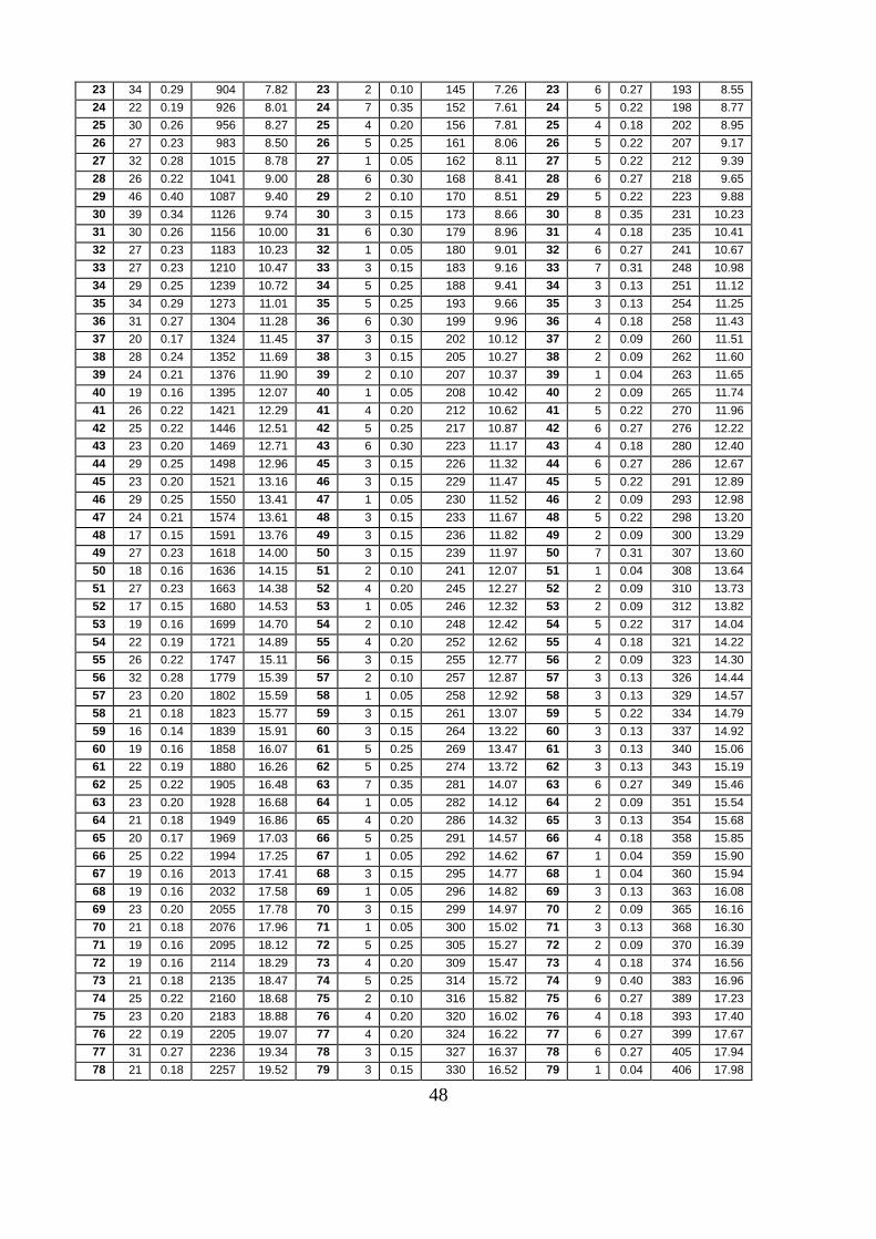
48
23 34 0.29 904 7.82 23 2 0.10 145 7.26 23 6 0.27 193 8.55
24 22 0.19 926 8.01 24 7 0.35 152 7.61 24 5 0.22 198 8.77
25 30 0.26 956 8.27 25 4 0.20 156 7.81 25 4 0.18 202 8.95
26 27 0.23 983 8.50 26 5 0.25 161 8.06 26 5 0.22 207 9.17
27 32 0.28 1015 8.78 27 1 0.05 162 8.11 27 5 0.22 212 9.39
28 26 0.22 1041 9.00 28 6 0.30 168 8.41 28 6 0.27 218 9.65
29 46 0.40 1087 9.40 29 2 0.10 170 8.51 29 5 0.22 223 9.88
30 39 0.34 1126 9.74 30 3 0.15 173 8.66 30 8 0.35 231 10.23
31 30 0.26 1156 10.00 31 6 0.30 179 8.96 31 4 0.18 235 10.41
32 27 0.23 1183 10.23 32 1 0.05 180 9.01 32 6 0.27 241 10.67
33 27 0.23 1210 10.47 33 3 0.15 183 9.16 33 7 0.31 248 10.98
34 29 0.25 1239 10.72 34 5 0.25 188 9.41 34 3 0.13 251 11.12
35 34 0.29 1273 11.01 35 5 0.25 193 9.66 35 3 0.13 254 11.25
36 31 0.27 1304 11.28 36 6 0.30 199 9.96 36 4 0.18 258 11.43
37 20 0.17 1324 11.45 37 3 0.15 202 10.12 37 2 0.09 260 11.51
38 28 0.24 1352 11.69 38 3 0.15 205 10.27 38 2 0.09 262 11.60
39 24 0.21 1376 11.90 39 2 0.10 207 10.37 39 1 0.04 263 11.65
40 19 0.16 1395 12.07 40 1 0.05 208 10.42 40 2 0.09 265 11.74
41 26 0.22 1421 12.29 41 4 0.20 212 10.62 41 5 0.22 270 11.96
42 25 0.22 1446 12.51 42 5 0.25 217 10.87 42 6 0.27 276 12.22
43 23 0.20 1469 12.71 43 6 0.30 223 11.17 43 4 0.18 280 12.40
44 29 0.25 1498 12.96 45 3 0.15 226 11.32 44 6 0.27 286 12.67
45 23 0.20 1521 13.16 46 3 0.15 229 11.47 45 5 0.22 291 12.89
46 29 0.25 1550 13.41 47 1 0.05 230 11.52 46 2 0.09 293 12.98
47 24 0.21 1574 13.61 48 3 0.15 233 11.67 48 5 0.22 298 13.20
48 17 0.15 1591 13.76 49 3 0.15 236 11.82 49 2 0.09 300 13.29
49 27 0.23 1618 14.00 50 3 0.15 239 11.97 50 7 0.31 307 13.60
50 18 0.16 1636 14.15 51 2 0.10 241 12.07 51 1 0.04 308 13.64
51 27 0.23 1663 14.38 52 4 0.20 245 12.27 52 2 0.09 310 13.73
52 17 0.15 1680 14.53 53 1 0.05 246 12.32 53 2 0.09 312 13.82
53 19 0.16 1699 14.70 54 2 0.10 248 12.42 54 5 0.22 317 14.04
54 22 0.19 1721 14.89 55 4 0.20 252 12.62 55 4 0.18 321 14.22
55 26 0.22 1747 15.11 56 3 0.15 255 12.77 56 2 0.09 323 14.30
56 32 0.28 1779 15.39 57 2 0.10 257 12.87 57 3 0.13 326 14.44
57 23 0.20 1802 15.59 58 1 0.05 258 12.92 58 3 0.13 329 14.57
58 21 0.18 1823 15.77 59 3 0.15 261 13.07 59 5 0.22 334 14.79
59 16 0.14 1839 15.91 60 3 0.15 264 13.22 60 3 0.13 337 14.92
60 19 0.16 1858 16.07 61 5 0.25 269 13.47 61 3 0.13 340 15.06
61 22 0.19 1880 16.26 62 5 0.25 274 13.72 62 3 0.13 343 15.19
62 25 0.22 1905 16.48 63 7 0.35 281 14.07 63 6 0.27 349 15.46
63 23 0.20 1928 16.68 64 1 0.05 282 14.12 64 2 0.09 351 15.54
64 21 0.18 1949 16.86 65 4 0.20 286 14.32 65 3 0.13 354 15.68
65 20 0.17 1969 17.03 66 5 0.25 291 14.57 66 4 0.18 358 15.85
66 25 0.22 1994 17.25 67 1 0.05 292 14.62 67 1 0.04 359 15.90
67 19 0.16 2013 17.41 68 3 0.15 295 14.77 68 1 0.04 360 15.94
68 19 0.16 2032 17.58 69 1 0.05 296 14.82 69 3 0.13 363 16.08
69 23 0.20 2055 17.78 70 3 0.15 299 14.97 70 2 0.09 365 16.16
70 21 0.18 2076 17.96 71 1 0.05 300 15.02 71 3 0.13 368 16.30
71 19 0.16 2095 18.12 72 5 0.25 305 15.27 72 2 0.09 370 16.39
72 19 0.16 2114 18.29 73 4 0.20 309 15.47 73 4 0.18 374 16.56
73 21 0.18 2135 18.47 74 5 0.25 314 15.72 74 9 0.40 383 16.96
74 25 0.22 2160 18.68 75 2 0.10 316 15.82 75 6 0.27 389 17.23
75 23 0.20 2183 18.88 76 4 0.20 320 16.02 76 4 0.18 393 17.40
76 22 0.19 2205 19.07 77 4 0.20 324 16.22 77 6 0.27 399 17.67
77 31 0.27 2236 19.34 78 3 0.15 327 16.37 78 6 0.27 405 17.94
78 21 0.18 2257 19.52 79 3 0.15 330 16.52 79 1 0.04 406 17.98
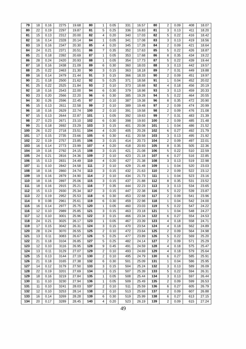
49
79 18 0.16 2275 19.68 80 1 0.05 331 16.57 80 2 0.09 408 18.07
80 22 0.19 2297 19.87 81 5 0.25 336 16.83 81 3 0.13 411 18.20
81 15 0.13 2312 20.00 82 4 0.20 340 17.03 82 5 0.22 416 18.42
82 16 0.14 2328 20.14 84 1 0.05 341 17.08 83 3 0.13 419 18.56
83 19 0.16 2347 20.30 85 4 0.20 345 17.28 84 2 0.09 421 18.64
84 24 0.21 2371 20.51 86 7 0.35 352 17.63 85 5 0.22 426 18.87
85 21 0.18 2392 20.69 87 1 0.05 353 17.68 86 8 0.35 434 19.22
86 28 0.24 2420 20.93 88 1 0.05 354 17.73 87 5 0.22 439 19.44
87 18 0.16 2438 21.09 89 6 0.30 360 18.03 88 3 0.13 442 19.57
88 25 0.22 2463 21.30 90 3 0.15 363 18.18 89 7 0.31 449 19.88
89 16 0.14 2479 21.44 91 3 0.15 366 18.33 90 2 0.09 451 19.97
90 21 0.18 2500 21.62 92 5 0.25 371 18.58 91 1 0.04 452 20.02
91 25 0.22 2525 21.84 93 2 0.10 373 18.68 92 4 0.18 456 20.19
92 18 0.16 2543 22.00 94 6 0.30 379 18.98 93 3 0.13 459 20.33
93 23 0.20 2566 22.20 96 6 0.30 385 19.28 94 5 0.22 464 20.55
94 30 0.26 2596 22.45 97 2 0.10 387 19.38 96 8 0.35 472 20.90
95 15 0.13 2611 22.58 99 2 0.10 389 19.48 97 2 0.09 474 20.99
96 18 0.16 2629 22.74 100 2 0.10 391 19.58 98 2 0.09 476 21.08
97 15 0.13 2644 22.87 101 1 0.05 392 19.63 99 7 0.31 483 21.39
98 27 0.23 2671 23.10 102 6 0.30 398 19.93 100 2 0.09 485 21.48
99 21 0.18 2692 23.29 103 3 0.15 401 20.08 101 1 0.04 486 21.52
100 26 0.22 2718 23.51 104 4 0.20 405 20.28 102 6 0.27 492 21.79
101 17 0.15 2735 23.66 105 6 0.30 411 20.58 103 3 0.13 495 21.92
102 22 0.19 2757 23.85 106 3 0.15 414 20.73 104 2 0.09 497 22.01
103 16 0.14 2773 23.99 107 4 0.20 418 20.93 105 8 0.35 505 22.36
104 19 0.16 2792 24.15 108 3 0.15 421 21.08 106 5 0.22 510 22.59
105 24 0.21 2816 24.36 109 2 0.10 423 21.18 107 6 0.27 516 22.85
106 15 0.13 2831 24.49 110 4 0.20 427 21.38 108 3 0.13 519 22.98
107 11 0.10 2842 24.58 111 2 0.10 429 21.48 109 1 0.04 520 23.03
108 18 0.16 2860 24.74 113 3 0.15 432 21.63 110 2 0.09 522 23.12
109 19 0.16 2879 24.90 114 2 0.10 434 21.73 111 1 0.04 523 23.16
110 18 0.16 2897 25.06 115 3 0.15 437 21.88 112 8 0.35 531 23.52
111 18 0.16 2915 25.21 116 7 0.35 444 22.23 113 3 0.13 534 23.65
112 15 0.13 2930 25.34 117 3 0.15 447 22.38 116 5 0.22 539 23.87
113 22 0.19 2952 25.53 118 6 0.30 453 22.68 117 2 0.09 541 23.96
114 9 0.08 2961 25.61 119 6 0.30 459 22.98 118 1 0.04 542 24.00
115 16 0.14 2977 25.75 120 1 0.05 460 23.03 119 5 0.22 547 24.22
116 12 0.10 2989 25.85 121 3 0.15 463 23.18 121 1 0.04 548 24.27
117 12 0.10 3001 25.96 122 3 0.15 466 23.34 122 6 0.27 554 24.53
118 24 0.21 3025 26.17 123 1 0.05 467 23.39 123 4 0.18 558 24.71
119 17 0.15 3042 26.31 124 3 0.15 470 23.54 124 4 0.18 562 24.89
120 28 0.24 3070 26.55 125 2 0.10 472 23.64 125 2 0.09 564 24.98
121 13 0.11 3083 26.67 126 5 0.25 477 23.89 126 5 0.22 569 25.20
122 21 0.18 3104 26.85 127 5 0.25 482 24.14 127 2 0.09 571 25.29
123 12 0.10 3116 26.95 128 9 0.45 491 24.59 128 4 0.18 575 25.47
124 13 0.11 3129 27.07 129 2 0.10 493 24.69 129 4 0.18 579 25.64
125 15 0.13 3144 27.19 130 2 0.10 495 24.79 130 6 0.27 585 25.91
126 21 0.18 3165 27.38 132 6 0.30 501 25.09 131 1 0.04 586 25.95
127 14 0.12 3179 27.50 133 3 0.15 504 25.24 132 3 0.13 589 26.09
128 22 0.19 3201 27.69 134 3 0.15 507 25.39 133 5 0.22 594 26.31
129 18 0.16 3219 27.84 135 1 0.05 508 25.44 134 3 0.13 597 26.44
130 11 0.10 3230 27.94 136 1 0.05 509 25.49 135 2 0.09 599 26.53
131 11 0.10 3241 28.03 137 2 0.10 511 25.59 136 6 0.27 605 26.79
132 12 0.10 3253 28.14 138 2 0.10 513 25.69 137 2 0.09 607 26.88
133 16 0.14 3269 28.28 139 6 0.30 519 25.99 138 6 0.27 613 27.15
134 20 0.17 3289 28.45 140 4 0.20 523 26.19 139 2 0.09 615 27.24
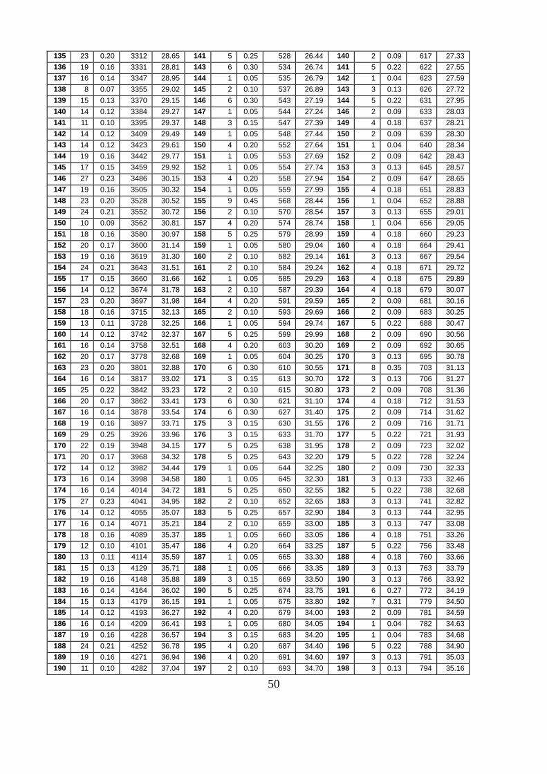
50
135 23 0.20 3312 28.65 141 5 0.25 528 26.44 140 2 0.09 617 27.33
136 19 0.16 3331 28.81 143 6 0.30 534 26.74 141 5 0.22 622 27.55
137 16 0.14 3347 28.95 144 1 0.05 535 26.79 142 1 0.04 623 27.59
138 8 0.07 3355 29.02 145 2 0.10 537 26.89 143 3 0.13 626 27.72
139 15 0.13 3370 29.15 146 6 0.30 543 27.19 144 5 0.22 631 27.95
140 14 0.12 3384 29.27 147 1 0.05 544 27.24 146 2 0.09 633 28.03
141 11 0.10 3395 29.37 148 3 0.15 547 27.39 149 4 0.18 637 28.21
142 14 0.12 3409 29.49 149 1 0.05 548 27.44 150 2 0.09 639 28.30
143 14 0.12 3423 29.61 150 4 0.20 552 27.64 151 1 0.04 640 28.34
144 19 0.16 3442 29.77 151 1 0.05 553 27.69 152 2 0.09 642 28.43
145 17 0.15 3459 29.92 152 1 0.05 554 27.74 153 3 0.13 645 28.57
146 27 0.23 3486 30.15 153 4 0.20 558 27.94 154 2 0.09 647 28.65
147 19 0.16 3505 30.32 154 1 0.05 559 27.99 155 4 0.18 651 28.83
148 23 0.20 3528 30.52 155 9 0.45 568 28.44 156 1 0.04 652 28.88
149 24 0.21 3552 30.72 156 2 0.10 570 28.54 157 3 0.13 655 29.01
150 10 0.09 3562 30.81 157 4 0.20 574 28.74 158 1 0.04 656 29.05
151 18 0.16 3580 30.97 158 5 0.25 579 28.99 159 4 0.18 660 29.23
152 20 0.17 3600 31.14 159 1 0.05 580 29.04 160 4 0.18 664 29.41
153 19 0.16 3619 31.30 160 2 0.10 582 29.14 161 3 0.13 667 29.54
154 24 0.21 3643 31.51 161 2 0.10 584 29.24 162 4 0.18 671 29.72
155 17 0.15 3660 31.66 162 1 0.05 585 29.29 163 4 0.18 675 29.89
156 14 0.12 3674 31.78 163 2 0.10 587 29.39 164 4 0.18 679 30.07
157 23 0.20 3697 31.98 164 4 0.20 591 29.59 165 2 0.09 681 30.16
158 18 0.16 3715 32.13 165 2 0.10 593 29.69 166 2 0.09 683 30.25
159 13 0.11 3728 32.25 166 1 0.05 594 29.74 167 5 0.22 688 30.47
160 14 0.12 3742 32.37 167 5 0.25 599 29.99 168 2 0.09 690 30.56
161 16 0.14 3758 32.51 168 4 0.20 603 30.20 169 2 0.09 692 30.65
162 20 0.17 3778 32.68 169 1 0.05 604 30.25 170 3 0.13 695 30.78
163 23 0.20 3801 32.88 170 6 0.30 610 30.55 171 8 0.35 703 31.13
164 16 0.14 3817 33.02 171 3 0.15 613 30.70 172 3 0.13 706 31.27
165 25 0.22 3842 33.23 172 2 0.10 615 30.80 173 2 0.09 708 31.36
166 20 0.17 3862 33.41 173 6 0.30 621 31.10 174 4 0.18 712 31.53
167 16 0.14 3878 33.54 174 6 0.30 627 31.40 175 2 0.09 714 31.62
168 19 0.16 3897 33.71 175 3 0.15 630 31.55 176 2 0.09 716 31.71
169 29 0.25 3926 33.96 176 3 0.15 633 31.70 177 5 0.22 721 31.93
170 22 0.19 3948 34.15 177 5 0.25 638 31.95 178 2 0.09 723 32.02
171 20 0.17 3968 34.32 178 5 0.25 643 32.20 179 5 0.22 728 32.24
172 14 0.12 3982 34.44 179 1 0.05 644 32.25 180 2 0.09 730 32.33
173 16 0.14 3998 34.58 180 1 0.05 645 32.30 181 3 0.13 733 32.46
174 16 0.14 4014 34.72 181 5 0.25 650 32.55 182 5 0.22 738 32.68
175 27 0.23 4041 34.95 182 2 0.10 652 32.65 183 3 0.13 741 32.82
176 14 0.12 4055 35.07 183 5 0.25 657 32.90 184 3 0.13 744 32.95
177 16 0.14 4071 35.21 184 2 0.10 659 33.00 185 3 0.13 747 33.08
178 18 0.16 4089 35.37 185 1 0.05 660 33.05 186 4 0.18 751 33.26
179 12 0.10 4101 35.47 186 4 0.20 664 33.25 187 5 0.22 756 33.48
180 13 0.11 4114 35.59 187 1 0.05 665 33.30 188 4 0.18 760 33.66
181 15 0.13 4129 35.71 188 1 0.05 666 33.35 189 3 0.13 763 33.79
182 19 0.16 4148 35.88 189 3 0.15 669 33.50 190 3 0.13 766 33.92
183 16 0.14 4164 36.02 190 5 0.25 674 33.75 191 6 0.27 772 34.19
184 15 0.13 4179 36.15 191 1 0.05 675 33.80 192 7 0.31 779 34.50
185 14 0.12 4193 36.27 192 4 0.20 679 34.00 193 2 0.09 781 34.59
186 16 0.14 4209 36.41 193 1 0.05 680 34.05 194 1 0.04 782 34.63
187 19 0.16 4228 36.57 194 3 0.15 683 34.20 195 1 0.04 783 34.68
188 24 0.21 4252 36.78 195 4 0.20 687 34.40 196 5 0.22 788 34.90
189 19 0.16 4271 36.94 196 4 0.20 691 34.60 197 3 0.13 791 35.03
190 11 0.10 4282 37.04 197 2 0.10 693 34.70 198 3 0.13 794 35.16
51
191 19 0.16 4301 37.20 198 1 0.05 694 34.75 199 1 0.04 795 35.21
192 11 0.10 4312 37.30 199 2 0.10 696 34.85 200 6 0.27 801 35.47
193 19 0.16 4331 37.46 200 1 0.05 697 34.90 201 5 0.22 806 35.70
194 25 0.22 4356 37.68 201 1 0.05 698 34.95 202 3 0.13 809 35.83
195 14 0.12 4370 37.80 202 1 0.05 699 35.00 203 3 0.13 812 35.96
196 22 0.19 4392 37.99 203 2 0.10 701 35.10 204 4 0.18 816 36.14
197 17 0.15 4409 38.14 204 5 0.25 706 35.35 205 2 0.09 818 36.23
198 16 0.14 4425 38.28 206 1 0.05 707 35.40 206 2 0.09 820 36.32
199 17 0.15 4442 38.42 207 4 0.20 711 35.60 207 3 0.13 823 36.45
200 18 0.16 4460 38.58 208 3 0.15 714 35.75 208 1 0.04 824 36.49
201 23 0.20 4483 38.78 209 5 0.25 719 36.00 209 3 0.13 827 36.63
202 18 0.16 4501 38.93 210 3 0.15 722 36.15 210 1 0.04 828 36.67
203 15 0.13 4516 39.06 211 2 0.10 724 36.25 211 2 0.09 830 36.76
204 17 0.15 4533 39.21 212 1 0.05 725 36.30 212 3 0.13 833 36.89
205 31 0.27 4564 39.48 213 2 0.10 727 36.40 213 4 0.18 837 37.07
206 17 0.15 4581 39.62 214 6 0.30 733 36.71 214 3 0.13 840 37.20
207 15 0.13 4596 39.75 215 6 0.30 739 37.01 215 2 0.09 842 37.29
208 17 0.15 4613 39.90 216 7 0.35 746 37.36 216 4 0.18 846 37.47
209 16 0.14 4629 40.04 217 6 0.30 752 37.66 217 4 0.18 850 37.64
210 22 0.19 4651 40.23 218 3 0.15 755 37.81 218 5 0.22 855 37.87
211 18 0.16 4669 40.39 219 2 0.10 757 37.91 219 3 0.13 858 38.00
212 16 0.14 4685 40.52 220 5 0.25 762 38.16 220 6 0.27 864 38.26
213 16 0.14 4701 40.66 221 4 0.20 766 38.36 221 5 0.22 869 38.49
214 18 0.16 4719 40.82 222 1 0.05 767 38.41 222 2 0.09 871 38.57
215 20 0.17 4739 40.99 223 3 0.15 770 38.56 223 2 0.09 873 38.66
216 18 0.16 4757 41.15 224 4 0.20 774 38.76 224 4 0.18 877 38.84
217 20 0.17 4777 41.32 225 3 0.15 777 38.91 225 3 0.13 880 38.97
218 16 0.14 4793 41.46 226 4 0.20 781 39.11 226 5 0.22 885 39.19
219 17 0.15 4810 41.61 227 2 0.10 783 39.21 227 3 0.13 888 39.33
220 20 0.17 4830 41.78 228 2 0.10 785 39.31 228 1 0.04 889 39.37
221 21 0.18 4851 41.96 229 4 0.20 789 39.51 229 3 0.13 892 39.50
222 19 0.16 4870 42.12 230 3 0.15 792 39.66 230 2 0.09 894 39.59
223 17 0.15 4887 42.27 231 5 0.25 797 39.91 231 4 0.18 898 39.77
224 20 0.17 4907 42.44 233 4 0.20 801 40.11 232 4 0.18 902 39.95
225 18 0.16 4925 42.60 234 4 0.20 805 40.31 234 6 0.27 908 40.21
226 12 0.10 4937 42.70 235 5 0.25 810 40.56 235 2 0.09 910 40.30
227 15 0.13 4952 42.83 236 2 0.10 812 40.66 236 3 0.13 913 40.43
228 16 0.14 4968 42.97 237 4 0.20 816 40.86 237 5 0.22 918 40.66
229 17 0.15 4985 43.12 238 1 0.05 817 40.91 238 3 0.13 921 40.79
230 13 0.11 4998 43.23 239 2 0.10 819 41.01 239 4 0.18 925 40.97
231 25 0.22 5023 43.45 240 4 0.20 823 41.21 240 4 0.18 929 41.14
232 24 0.21 5047 43.66 241 3 0.15 826 41.36 241 3 0.13 932 41.28
233 22 0.19 5069 43.85 242 4 0.20 830 41.56 242 1 0.04 933 41.32
234 12 0.10 5081 43.95 243 4 0.20 834 41.76 243 1 0.04 934 41.36
235 14 0.12 5095 44.07 245 2 0.10 836 41.86 244 3 0.13 937 41.50
236 24 0.21 5119 44.28 246 2 0.10 838 41.96 245 3 0.13 940 41.63
237 15 0.13 5134 44.41 247 2 0.10 840 42.06 246 2 0.09 942 41.72
238 19 0.16 5153 44.57 248 3 0.15 843 42.21 247 3 0.13 945 41.85
239 31 0.27 5184 44.84 249 4 0.20 847 42.41 248 5 0.22 950 42.07
240 13 0.11 5197 44.95 250 2 0.10 849 42.51 249 3 0.13 953 42.21
241 12 0.10 5209 45.06 251 2 0.10 851 42.61 250 5 0.22 958 42.43
242 28 0.24 5237 45.30 252 3 0.15 854 42.76 251 3 0.13 961 42.56
243 20 0.17 5257 45.47 253 5 0.25 859 43.01 252 5 0.22 966 42.78
244 17 0.15 5274 45.62 254 7 0.35 866 43.37 253 10 0.44 976 43.22
245 20 0.17 5294 45.79 256 5 0.25 871 43.62 254 2 0.09 978 43.31
246 16 0.14 5310 45.93 257 2 0.10 873 43.72 255 6 0.27 984 43.58
52
247 23 0.20 5333 46.13 258 2 0.10 875 43.82 256 2 0.09 986 43.67
248 11 0.10 5344 46.22 259 4 0.20 879 44.02 257 3 0.13 989 43.80
249 12 0.10 5356 46.33 260 2 0.10 881 44.12 258 3 0.13 992 43.93
250 16 0.14 5372 46.47 261 1 0.05 882 44.17 259 7 0.31 999 44.24
251 22 0.19 5394 46.66 262 1 0.05 883 44.22 260 5 0.22 1004 44.46
252 14 0.12 5408 46.78 263 3 0.15 886 44.37 261 1 0.04 1005 44.51
253 21 0.18 5429 46.96 264 1 0.05 887 44.42 262 6 0.27 1011 44.77
254 18 0.16 5447 47.12 265 4 0.20 891 44.62 263 4 0.18 1015 44.95
255 15 0.13 5462 47.25 266 1 0.05 892 44.67 264 4 0.18 1019 45.13
256 13 0.11 5475 47.36 267 2 0.10 894 44.77 265 5 0.22 1024 45.35
257 20 0.17 5495 47.53 268 1 0.05 895 44.82 266 1 0.04 1025 45.39
258 17 0.15 5512 47.68 270 3 0.15 898 44.97 268 3 0.13 1028 45.53
259 15 0.13 5527 47.81 272 1 0.05 899 45.02 269 8 0.35 1036 45.88
260 21 0.18 5548 47.99 273 5 0.25 904 45.27 270 1 0.04 1037 45.93
261 12 0.10 5560 48.09 274 3 0.15 907 45.42 272 5 0.22 1042 46.15
262 23 0.20 5583 48.29 275 3 0.15 910 45.57 273 6 0.27 1048 46.41
263 10 0.09 5593 48.38 276 2 0.10 912 45.67 274 4 0.18 1052 46.59
264 14 0.12 5607 48.50 277 3 0.15 915 45.82 275 3 0.13 1055 46.72
265 14 0.12 5621 48.62 278 1 0.05 916 45.87 276 4 0.18 1059 46.90
266 16 0.14 5637 48.76 279 3 0.15 919 46.02 277 2 0.09 1061 46.99
267 15 0.13 5652 48.89 280 4 0.20 923 46.22 278 3 0.13 1064 47.12
268 20 0.17 5672 49.06 281 2 0.10 925 46.32 279 1 0.04 1065 47.17
269 12 0.10 5684 49.17 282 3 0.15 928 46.47 280 4 0.18 1069 47.34
270 14 0.12 5698 49.29 283 4 0.20 932 46.67 281 4 0.18 1073 47.52
271 20 0.17 5718 49.46 284 3 0.15 935 46.82 282 2 0.09 1075 47.61
272 11 0.10 5729 49.55 285 1 0.05 936 46.87 284 3 0.13 1078 47.74
273 15 0.13 5744 49.68 286 4 0.20 940 47.07 285 5 0.22 1083 47.96
274 14 0.12 5758 49.81 287 3 0.15 943 47.22 286 3 0.13 1086 48.10
275 12 0.10 5770 49.91 288 4 0.20 947 47.42 287 4 0.18 1090 48.27
276 10 0.09 5780 50.00 289 7 0.35 954 47.77 288 1 0.04 1091 48.32
277 10 0.09 5790 50.08 290 5 0.25 959 48.02 289 2 0.09 1093 48.41
278 24 0.21 5814 50.29 291 6 0.30 965 48.32 290 5 0.22 1098 48.63
279 18 0.16 5832 50.45 292 3 0.15 968 48.47 291 2 0.09 1100 48.72
280 19 0.16 5851 50.61 293 1 0.05 969 48.52 292 6 0.27 1106 48.98
281 23 0.20 5874 50.81 294 4 0.20 973 48.72 293 5 0.22 1111 49.20
282 20 0.17 5894 50.98 295 5 0.25 978 48.97 294 4 0.18 1115 49.38
283 15 0.13 5909 51.11 296 5 0.25 983 49.22 295 4 0.18 1119 49.56
284 15 0.13 5924 51.24 297 1 0.05 984 49.27 296 3 0.13 1122 49.69
285 16 0.14 5940 51.38 298 5 0.25 989 49.52 297 4 0.18 1126 49.87
286 15 0.13 5955 51.51 299 2 0.10 991 49.62 298 2 0.09 1128 49.96
287 19 0.16 5974 51.67 301 4 0.20 995 49.82 299 1 0.04 1129 50.00
288 16 0.14 5990 51.81 302 3 0.15 998 49.97 300 2 0.09 1131 50.09
289 19 0.16 6009 51.98 303 2 0.10 1000 50.08 301 6 0.27 1137 50.35
290 20 0.17 6029 52.15 305 3 0.15 1003 50.23 302 2 0.09 1139 50.44
291 25 0.22 6054 52.37 306 3 0.15 1006 50.38 303 2 0.09 1141 50.53
292 24 0.21 6078 52.57 307 5 0.25 1011 50.63 304 3 0.13 1144 50.66
293 16 0.14 6094 52.71 308 5 0.25 1016 50.88 305 6 0.27 1150 50.93
294 22 0.19 6116 52.90 309 6 0.30 1022 51.18 306 3 0.13 1153 51.06
295 13 0.11 6129 53.01 310 4 0.20 1026 51.38 307 2 0.09 1155 51.15
296 17 0.15 6146 53.16 311 3 0.15 1029 51.53 308 6 0.27 1161 51.42
297 18 0.16 6164 53.32 312 5 0.25 1034 51.78 309 5 0.22 1166 51.64
298 19 0.16 6183 53.48 313 6 0.30 1040 52.08 310 4 0.18 1170 51.82
299 14 0.12 6197 53.60 314 3 0.15 1043 52.23 311 4 0.18 1174 51.99
300 16 0.14 6213 53.74 315 3 0.15 1046 52.38 312 4 0.18 1178 52.17
301 17 0.15 6230 53.89 316 4 0.20 1050 52.58 313 4 0.18 1182 52.35
302 17 0.15 6247 54.04 317 4 0.20 1054 52.78 314 5 0.22 1187 52.57
53
303 16 0.14 6263 54.17 318 3 0.15 1057 52.93 315 2 0.09 1189 52.66
304 21 0.18 6284 54.36 319 8 0.40 1065 53.33 316 5 0.22 1194 52.88
305 18 0.16 6302 54.51 320 3 0.15 1068 53.48 317 3 0.13 1197 53.01
306 12 0.10 6314 54.61 321 4 0.20 1072 53.68 318 5 0.22 1202 53.23
307 17 0.15 6331 54.76 322 4 0.20 1076 53.88 319 6 0.27 1208 53.50
308 17 0.15 6348 54.91 323 3 0.15 1079 54.03 320 2 0.09 1210 53.59
309 18 0.16 6366 55.06 324 1 0.05 1080 54.08 321 1 0.04 1211 53.63
310 20 0.17 6386 55.24 325 1 0.05 1081 54.13 322 6 0.27 1217 53.90
311 16 0.14 6402 55.38 326 4 0.20 1085 54.33 323 5 0.22 1222 54.12
312 19 0.16 6421 55.54 328 1 0.05 1086 54.38 324 5 0.22 1227 54.34
313 19 0.16 6440 55.70 330 3 0.15 1089 54.53 325 3 0.13 1230 54.47
314 22 0.19 6462 55.89 331 3 0.15 1092 54.68 326 10 0.44 1240 54.92
315 25 0.22 6487 56.11 333 3 0.15 1095 54.83 327 6 0.27 1246 55.18
316 17 0.15 6504 56.26 334 2 0.10 1097 54.93 328 5 0.22 1251 55.40
317 16 0.14 6520 56.40 335 5 0.25 1102 55.18 329 3 0.13 1254 55.54
318 24 0.21 6544 56.60 336 4 0.20 1106 55.38 330 6 0.27 1260 55.80
319 14 0.12 6558 56.73 337 2 0.10 1108 55.48 331 2 0.09 1262 55.89
320 20 0.17 6578 56.90 338 2 0.10 1110 55.58 333 7 0.31 1269 56.20
321 15 0.13 6593 57.03 339 6 0.30 1116 55.88 334 1 0.04 1270 56.24
322 21 0.18 6614 57.21 340 3 0.15 1119 56.03 335 8 0.35 1278 56.60
323 22 0.19 6636 57.40 341 5 0.25 1124 56.28 336 2 0.09 1280 56.69
324 20 0.17 6656 57.57 342 4 0.20 1128 56.48 337 4 0.18 1284 56.86
325 17 0.15 6673 57.72 343 5 0.25 1133 56.74 338 1 0.04 1285 56.91
326 18 0.16 6691 57.88 344 6 0.30 1139 57.04 339 5 0.22 1290 57.13
327 19 0.16 6710 58.04 345 3 0.15 1142 57.19 340 2 0.09 1292 57.22
328 18 0.16 6728 58.20 346 3 0.15 1145 57.34 341 4 0.18 1296 57.40
329 28 0.24 6756 58.44 347 2 0.10 1147 57.44 342 3 0.13 1299 57.53
330 14 0.12 6770 58.56 348 2 0.10 1149 57.54 343 5 0.22 1304 57.75
331 27 0.23 6797 58.79 349 1 0.05 1150 57.59 344 12 0.53 1316 58.28
332 21 0.18 6818 58.97 350 5 0.25 1155 57.84 345 2 0.09 1318 58.37
333 19 0.16 6837 59.14 351 1 0.05 1156 57.89 346 5 0.22 1323 58.59
334 15 0.13 6852 59.27 352 4 0.20 1160 58.09 347 6 0.27 1329 58.86
335 20 0.17 6872 59.44 353 3 0.15 1163 58.24 348 5 0.22 1334 59.08
336 18 0.16 6890 59.60 354 3 0.15 1166 58.39 349 6 0.27 1340 59.34
337 9 0.08 6899 59.67 355 5 0.25 1171 58.64 350 3 0.13 1343 59.48
338 22 0.19 6921 59.87 356 7 0.35 1178 58.99 351 3 0.13 1346 59.61
339 20 0.17 6941 60.04 357 5 0.25 1183 59.24 352 5 0.22 1351 59.83
340 23 0.20 6964 60.24 358 2 0.10 1185 59.34 353 1 0.04 1352 59.88
341 17 0.15 6981 60.38 359 2 0.10 1187 59.44 354 6 0.27 1358 60.14
342 22 0.19 7003 60.57 360 3 0.15 1190 59.59 355 6 0.27 1364 60.41
343 25 0.22 7028 60.79 361 5 0.25 1195 59.84 356 1 0.04 1365 60.45
344 23 0.20 7051 60.99 362 3 0.15 1198 59.99 357 7 0.31 1372 60.76
345 20 0.17 7071 61.16 363 4 0.20 1202 60.19 358 3 0.13 1375 60.89
346 16 0.14 7087 61.30 364 4 0.20 1206 60.39 359 1 0.04 1376 60.94
347 16 0.14 7103 61.44 365 1 0.05 1207 60.44 360 5 0.22 1381 61.16
348 14 0.12 7117 61.56 366 8 0.40 1215 60.84 361 1 0.04 1382 61.20
349 24 0.21 7141 61.77 367 5 0.25 1220 61.09 362 4 0.18 1386 61.38
350 19 0.16 7160 61.93 368 6 0.30 1226 61.39 363 2 0.09 1388 61.47
351 25 0.22 7185 62.15 369 1 0.05 1227 61.44 364 5 0.22 1393 61.69
352 23 0.20 7208 62.35 370 5 0.25 1232 61.69 365 6 0.27 1399 61.96
353 17 0.15 7225 62.49 371 3 0.15 1235 61.84 366 1 0.04 1400 62.00
354 19 0.16 7244 62.66 372 4 0.20 1239 62.04 367 5 0.22 1405 62.22
355 14 0.12 7258 62.78 373 3 0.15 1242 62.19 368 4 0.18 1409 62.40
356 10 0.09 7268 62.87 374 5 0.25 1247 62.44 369 1 0.04 1410 62.44
357 15 0.13 7283 63.00 375 1 0.05 1248 62.49 370 3 0.13 1413 62.58
358 13 0.11 7296 63.11 376 2 0.10 1250 62.59 371 2 0.09 1415 62.67
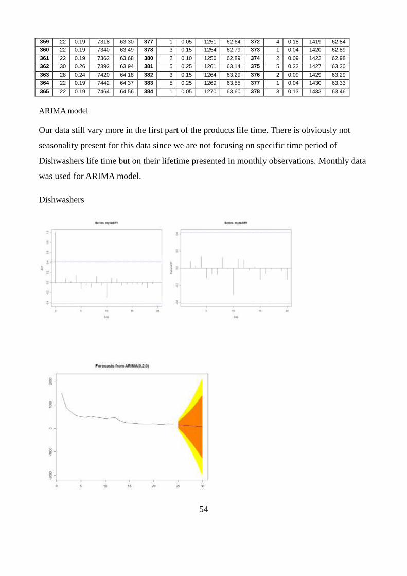
54
359 22 0.19 7318 63.30 377 1 0.05 1251 62.64 372 4 0.18 1419 62.84
360 22 0.19 7340 63.49 378 3 0.15 1254 62.79 373 1 0.04 1420 62.89
361 22 0.19 7362 63.68 380 2 0.10 1256 62.89 374 2 0.09 1422 62.98
362 30 0.26 7392 63.94 381 5 0.25 1261 63.14 375 5 0.22 1427 63.20
363 28 0.24 7420 64.18 382 3 0.15 1264 63.29 376 2 0.09 1429 63.29
364 22 0.19 7442 64.37 383 5 0.25 1269 63.55 377 1 0.04 1430 63.33
365 22 0.19 7464 64.56 384 1 0.05 1270 63.60 378 3 0.13 1433 63.46
ARIMA model
Our data still vary more in the first part of the products life time. There is obviously not
seasonality present for this data since we are not focusing on specific time period of
Dishwashers life time but on their lifetime presented in monthly observations. Monthly data
was used for ARIMA model.
Dishwashers
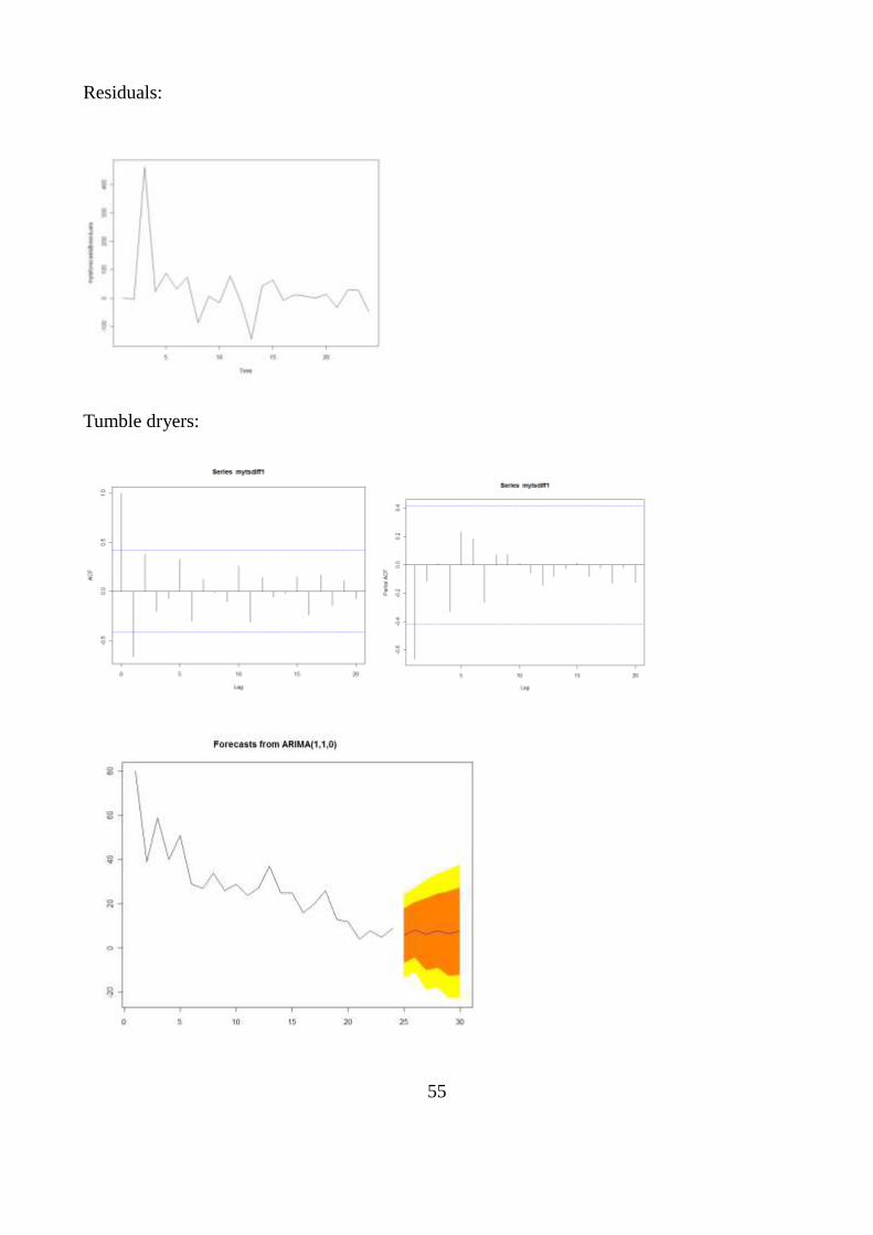
55
Residuals:
Tumble dryers:
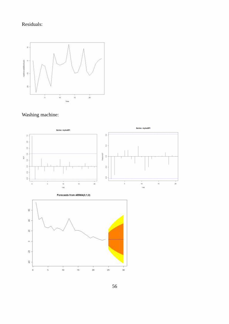
56
Residuals:
Washing machine:
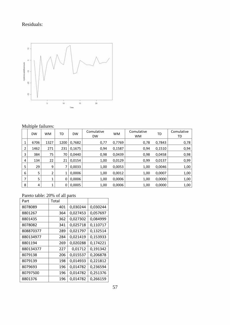
57
Residuals:
Multiple failures:
DW WM TD DW
Comulative DW
WM Comulative
WM TD
Comulative TD
1 6706 1327 1200 0,7682 0,77 0,7769 0,78 0,7843 0,78
2 1462 271 231 0,1675 0,94 0,1587 0,94 0,1510 0,94
3 384 75 70 0,0440 0,98 0,0439 0,98 0,0458 0,98
4 134 22 21 0,0154 1,00 0,0129 0,99 0,0137 0,99
5 29 9 7 0,0033 1,00 0,0053 1,00 0,0046 1,00
6 5 2 1 0,0006 1,00 0,0012 1,00 0,0007 1,00
7 5 1 0 0,0006 1,00 0,0006 1,00 0,0000 1,00
8 4 1 0 0,0005 1,00 0,0006 1,00 0,0000 1,00
Pareto table: 20% of all parts
Part Total
8078089 401 0,030244 0,030244
8801267 364 0,027453 0,057697
8801435 362 0,027302 0,084999
8078082 341 0,025718 0,110717
808870377 289 0,021797 0,132514
880134977 284 0,021419 0,153933
8801194 269 0,020288 0,174221
880134377 227 0,01712 0,191342
8079138 206 0,015537 0,206878
8079139 198 0,014933 0,221812
8079693 196 0,014782 0,236594
80797500 196 0,014782 0,251376
8801376 196 0,014782 0,266159
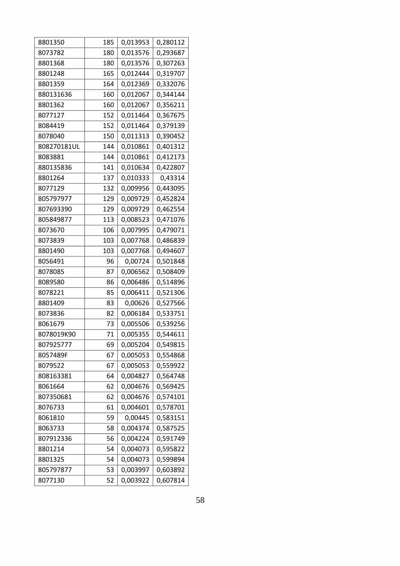
58
8801350 185 0,013953 0,280112
8073782 180 0,013576 0,293687
8801368 180 0,013576 0,307263
8801248 165 0,012444 0,319707
8801359 164 0,012369 0,332076
880131636 160 0,012067 0,344144
8801362 160 0,012067 0,356211
8077127 152 0,011464 0,367675
8084419 152 0,011464 0,379139
8078040 150 0,011313 0,390452
808270181UL 144 0,010861 0,401312
8083881 144 0,010861 0,412173
880135836 141 0,010634 0,422807
8801264 137 0,010333 0,43314
8077129 132 0,009956 0,443095
805797977 129 0,009729 0,452824
807693390 129 0,009729 0,462554
805849877 113 0,008523 0,471076
8073670 106 0,007995 0,479071
8073839 103 0,007768 0,486839
8801490 103 0,007768 0,494607
8056491 96 0,00724 0,501848
8078085 87 0,006562 0,508409
8089580 86 0,006486 0,514896
8078221 85 0,006411 0,521306
8801409 83 0,00626 0,527566
8073836 82 0,006184 0,533751
8061679 73 0,005506 0,539256
8078019K90 71 0,005355 0,544611
807925777 69 0,005204 0,549815
8057489F 67 0,005053 0,554868
8079522 67 0,005053 0,559922
808163381 64 0,004827 0,564748
8061664 62 0,004676 0,569425
807350681 62 0,004676 0,574101
8076733 61 0,004601 0,578701
8061810 59 0,00445 0,583151
8063733 58 0,004374 0,587525
807912336 56 0,004224 0,591749
8801214 54 0,004073 0,595822
8801325 54 0,004073 0,599894
805797877 53 0,003997 0,603892
8077130 52 0,003922 0,607814
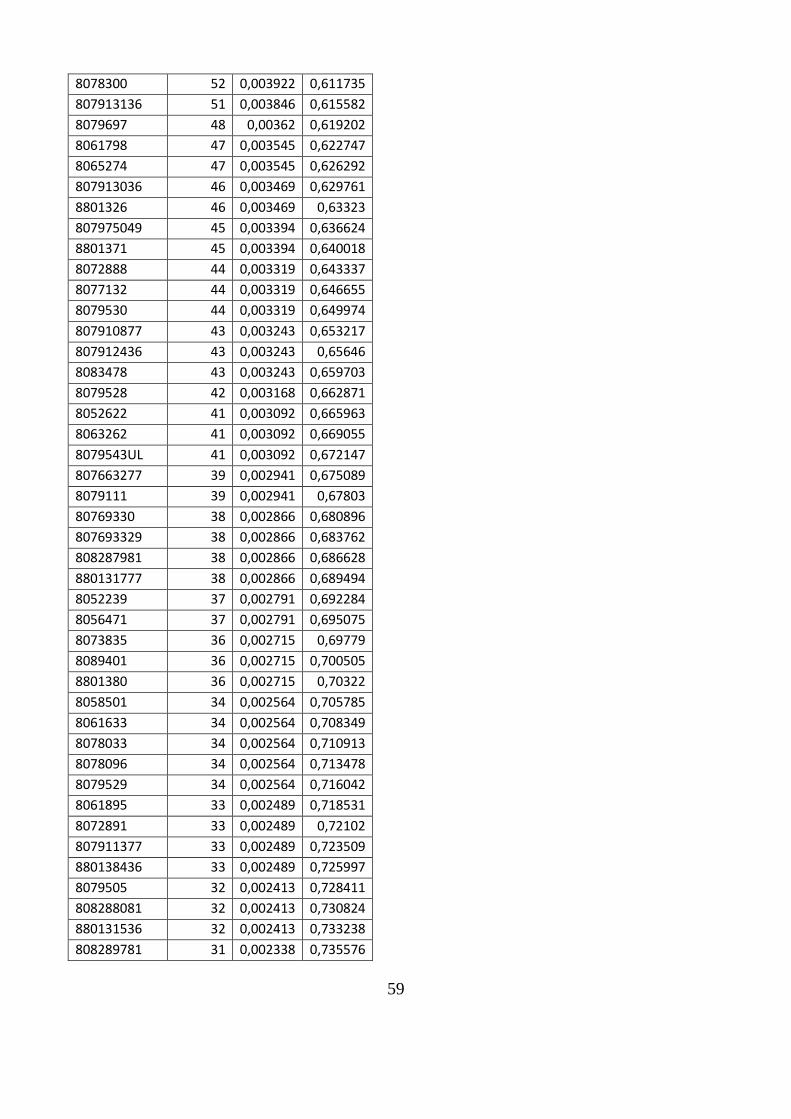
59
8078300 52 0,003922 0,611735
807913136 51 0,003846 0,615582
8079697 48 0,00362 0,619202
8061798 47 0,003545 0,622747
8065274 47 0,003545 0,626292
807913036 46 0,003469 0,629761
8801326 46 0,003469 0,63323
807975049 45 0,003394 0,636624
8801371 45 0,003394 0,640018
8072888 44 0,003319 0,643337
8077132 44 0,003319 0,646655
8079530 44 0,003319 0,649974
807910877 43 0,003243 0,653217
807912436 43 0,003243 0,65646
8083478 43 0,003243 0,659703
8079528 42 0,003168 0,662871
8052622 41 0,003092 0,665963
8063262 41 0,003092 0,669055
8079543UL 41 0,003092 0,672147
807663277 39 0,002941 0,675089
8079111 39 0,002941 0,67803
80769330 38 0,002866 0,680896
807693329 38 0,002866 0,683762
808287981 38 0,002866 0,686628
880131777 38 0,002866 0,689494
8052239 37 0,002791 0,692284
8056471 37 0,002791 0,695075
8073835 36 0,002715 0,69779
8089401 36 0,002715 0,700505
8801380 36 0,002715 0,70322
8058501 34 0,002564 0,705785
8061633 34 0,002564 0,708349
8078033 34 0,002564 0,710913
8078096 34 0,002564 0,713478
8079529 34 0,002564 0,716042
8061895 33 0,002489 0,718531
8072891 33 0,002489 0,72102
807911377 33 0,002489 0,723509
880138436 33 0,002489 0,725997
8079505 32 0,002413 0,728411
808288081 32 0,002413 0,730824
880131536 32 0,002413 0,733238
808289781 31 0,002338 0,735576
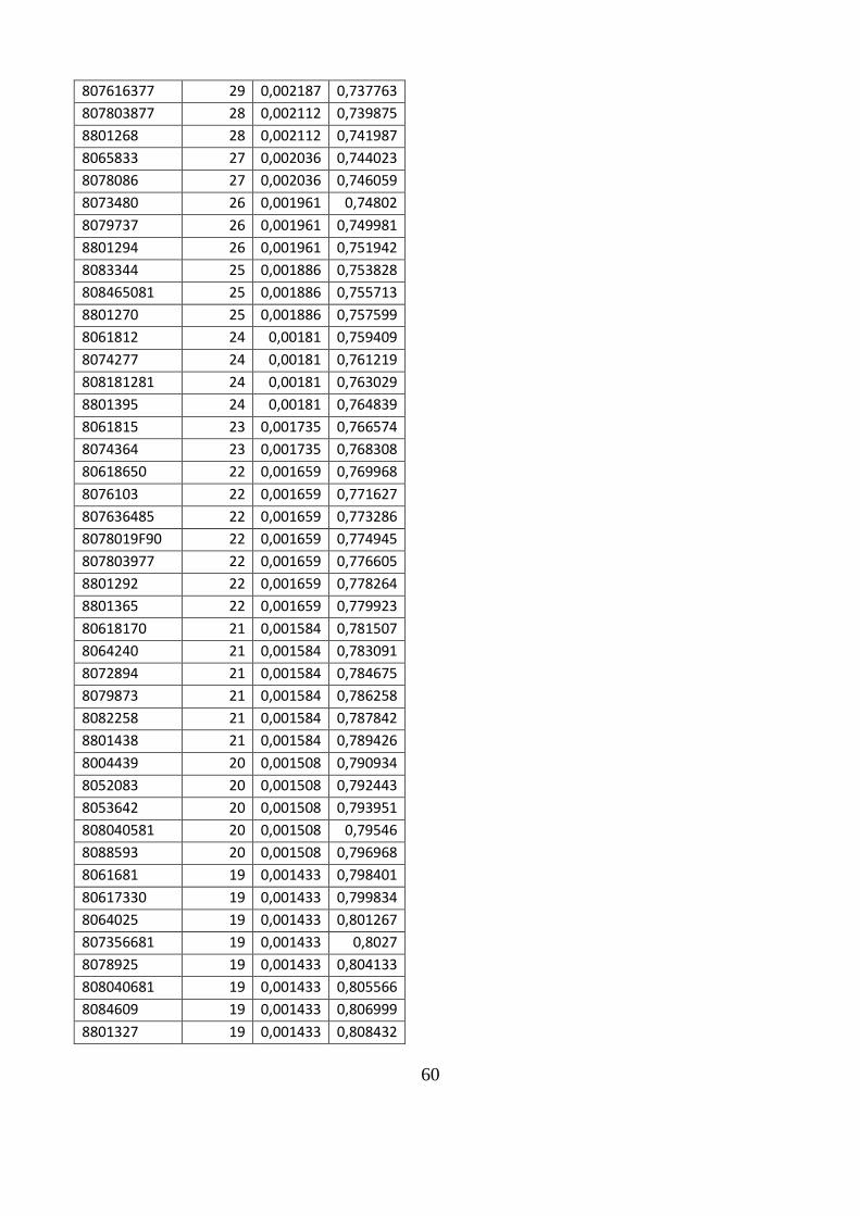
60
807616377 29 0,002187 0,737763
807803877 28 0,002112 0,739875
8801268 28 0,002112 0,741987
8065833 27 0,002036 0,744023
8078086 27 0,002036 0,746059
8073480 26 0,001961 0,74802
8079737 26 0,001961 0,749981
8801294 26 0,001961 0,751942
8083344 25 0,001886 0,753828
808465081 25 0,001886 0,755713
8801270 25 0,001886 0,757599
8061812 24 0,00181 0,759409
8074277 24 0,00181 0,761219
808181281 24 0,00181 0,763029
8801395 24 0,00181 0,764839
8061815 23 0,001735 0,766574
8074364 23 0,001735 0,768308
80618650 22 0,001659 0,769968
8076103 22 0,001659 0,771627
807636485 22 0,001659 0,773286
8078019F90 22 0,001659 0,774945
807803977 22 0,001659 0,776605
8801292 22 0,001659 0,778264
8801365 22 0,001659 0,779923
80618170 21 0,001584 0,781507
8064240 21 0,001584 0,783091
8072894 21 0,001584 0,784675
8079873 21 0,001584 0,786258
8082258 21 0,001584 0,787842
8801438 21 0,001584 0,789426
8004439 20 0,001508 0,790934
8052083 20 0,001508 0,792443
8053642 20 0,001508 0,793951
808040581 20 0,001508 0,79546
8088593 20 0,001508 0,796968
8061681 19 0,001433 0,798401
80617330 19 0,001433 0,799834
8064025 19 0,001433 0,801267
807356681 19 0,001433 0,8027
8078925 19 0,001433 0,804133
808040681 19 0,001433 0,805566
8084609 19 0,001433 0,806999
8801327 19 0,001433 0,808432
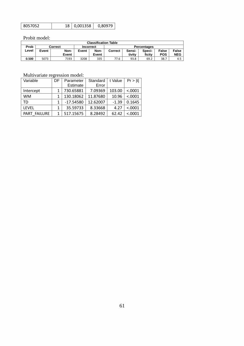
61
8057052 18 0,001358 0,80979
Probit model: Classification Table
Prob Level
Correct Incorrect Percentages
Event Non- Event
Event Non- Event
Correct Sensi- tivity
Speci- ficity
False POS
False NEG
0.500 5073 7193 3208 335 77.6 93.8 69.2 38.7 4.5
Multivariate regression model: Variable DF Parameter
Estimate Standard
Error t Value Pr > |t|
Intercept 1 730.65881 7.09369 103.00 <.0001
WM 1 130.18062 11.87680 10.96 <.0001
TD 1 -17.54580 12.62007 -1.39 0.1645
LEVEL 1 35.59733 8.33668 4.27 <.0001
PART_FAILURE 1 517.15675 8.28492 62.42 <.0001
Datum
Date
2013-06-17
Språk
Language
Svenska/Swedish
Engelska/English
Rapporttyp
Report category
Licentiatavhandling
Examensarbete
C-uppsats
D-uppsats
Övrig rapport
ISBN
ISRN
LIU-IDA/STAT-A--13/005--SE
Serietitel och serienummer ISSN
Title of series, numbering
URL för elektronisk version
Titel
Title
Warranty claims analysis for household appliances produced by ASKO Appliances AB
Författare
Author
Ana Turk
Sammanfattning
Abstract
The input collected from warranty claims data links customer feedback with product quality. Results from warranty
claim analysis can potentially improve product quality, customer relationships and positively affect business.
However working on warranty claims data holds many challenges that requires a significant share of time devoted
to data cleaning and data processing.
The purpose of warranty claims analysis is to get the comprehensive overview of the reliability, costs and quality of
household appliances produced by ASKO. While there are different ways to approach this problem, we will focus
on non-parametric and semi-parametric methods, by using Kaplan-Meier estimators and Cox proportional hazard
model respectively. These kinds of models are time dependent and therefore used for prediction of household
appliance reliability. Even though non-parametric models are quite informative they cannot handle additional
characteristics about observable product hence the semi-parametric Cox proportional hazard model was proposed.
Apart from the reliability analysis, we will also predict warranty costs with probit model and observe inequality in
household appliances part failures as a part of quality control analysis. Described methods were selected due to the
fact that the warranty claims analysis will be practiced in future by ASKO’s quality department and therefore
straight forward methods with very informative results are needed.
Nyckelord Keyword
Household appliances, warranty claims, reliability analysis, Cox proportional hazard model, marginal Cox model,
probit model, Pareto rule
Avdelning, Institution
Division, Department
Department of Computer and Information Science

LIU-IDA/STAT-A--13/005--SE