Was von Thünen right?

Cattle intensification and

deforestation in Brazil

Francisco Fontes and Charles Palmer

January 2017

Centre for Climate Change Economics and Policy Working Paper No. 294

Grantham Research Institute on Climate Change and the Environment Working Paper No. 261

This working paper is intended to stimulate discussion within the research community and among users of research, and its content may have

been submitted for publication in academic journals. It has been reviewed by at least one internal referee before publication. The views

expressed in this paper represent those of the author(s) and do not necessarily represent those of the host institutions or funders.

The Centre for Climate Change Economics and Policy (CCCEP) was established by the University of Leeds and the London

School of Economics and Political Science in 2008 to advance public and private action on climate change through innovative,

rigorous research. The Centre is funded by the UK Economic and Social Research Council. Its second phase started in 2013 and

there are five integrated research themes:

1. Understanding green growth and climate-compatible development

2. Advancing climate finance and investment

3. Evaluating the performance of climate policies

4. Managing climate risks and uncertainties and strengthening climate services

5. Enabling rapid transitions in mitigation and adaptation

More information about the Centre for Climate Change Economics and Policy can be found at: http://www.cccep.ac.uk.

The Grantham Research Institute on Climate Change and the Environment was established by the London School of

Economics and Political Science in 2008 to bring together international expertise on economics, finance, geography, the

environment, international development and political economy to create a world-leading centre for policy-relevant research and

training. The Institute is funded by the Grantham Foundation for the Protection of the Environment and the Global Green Growth

Institute. It has nine research programmes:

1. Adaptation and development

2. Carbon trading and finance

3. Ecosystems, resources and the natural environment

4. Energy, technology and trade

5. Future generations and social justice

6. Growth and the economy

7. International environmental negotiations

8. Modelling and decision making

9. Private sector adaptation, risk and insurance

More information about the Grantham Research Institute on Climate Change and the Environment can be found at:

http://www.lse.ac.uk/grantham.

1

WAS VON THÜNEN RIGHT?

CATTLE INTENSIFICATION AND DEFORESTATION IN BRAZIL1

Francisco Fontes2 and Charles Palmer3

Department of Geography and Environment & Grantham Research Institute on Climate Change and

the Environment

London School of Economics (LSE)

DRAFT – January 2017

ABSTRACT

This paper examines whether patterns of cattle intensification,

deforestation, and pasture expansion in the Brazilian state of Rondônia are

consistent with the land rent framework, in which location and distance to

markets is a key determinant of rents. A panel dataset of household lots,

collected between 1996 and 2009, is used to test the hypothesis that the

further a household is from market the more likely it will extensify cattle

production, deforest, and expand pasture in response to rising demand for

beef and milk. Results from a fixed effects model suggest empirical support

for the theory. Pasture area is significantly increasing while forest is

significantly decreasing in lots located further away from the market

relative to those closer to the market. Patterns of land use differ, however,

depending upon the forest type and commodity considered. Primary forest

may be ‘spared’ closer to market though perhaps at the cost of greater

conversion of secondary forest. Households with greater endowments of

forest tend to deforest more than those with smaller ones.

Keywords: Agriculture, Cattle, Deforestation, Households, Intensification, Land Rents, Sparing

JEL classification: Q12, Q15, Q23, Q24

_______________________________

1 Acknowledgements: We wish to thank the authors of the dataset (Caviglia-Harris, J. L., Roberts, D. and Sills, E.

O.), in particular, Jill Caviglia-Harris for sharing additional data, as well as the ICPSR (the distributor) for making

this dataset publicly available. We also thank David Simpson for useful comments on an early draft, and

comments from Mikolaj Czajkowski, Philippe Delacote, Silke Heuser, Katrina Mullan, Ingmar Schumacher, Daan

van Soest, and Eduardo Souza-Rodrigues, along with other participants at workshops organised by the

Laboratory of Forest Economics (Nice) and the French National Institute for Agricultural Research, INRA

(Montpellier), as well as those at the 18th Annual BIOECON Conference (Cambridge) and the Environmental

Economics seminar series hosted by AREC (Maryland). Francisco Fontes acknowledges support from the Centre for Climate Change Economics and Policy, which is funded by the UK Economic and Social Research Council.2 F.Pereira-Fontes@lse.ac.uk

3 C.palmer1@lse.ac.uk

2

1. INTRODUCTION

Growth in demand for meat and dairy products, particularly in emerging market economies such as

Brazil and China, has driven a huge rise in global livestock numbers. This, in turn, has had critical

implications for land use change. In the Brazilian Amazon, expanding cattle populations and pasture

areas as well as crop expansion are largely responsible for decades of deforestation (FAO, 2010;

Nepstad et al., 2009). To counter this expansion while continuing to meet the demand for food,

agricultural intensification is often promoted as a means of reducing cultivated areas, concentrating

production and allowing some lands to be ‘spared’ (e.g. Cohn et al., 2014; Nepstad et al., 2009;

Rudel et al., 2009). Between 1975 and 2006, this pattern is observed at the municipality scale in

‘agriculturally consolidated’ areas in the south of Brazil but not in Amazon forest frontier areas,

where intensification occurred alongside agricultural expansion (Barretto et al., 2013).

In this paper, we evaluate the extent to which patterns of intensification and land use among rural

households in the Amazon state of Rondônia are consistent with the land rent framework. Given

rapid ‘frontier urbanization’ and the establishment of close to 1,000 urban centres in the Brazilian

Amazon over the past 50 years (Browder and Godfrey, 1997; Brondizio, 2016),1 this framework

provides a useful basis for understanding land-use patterns at the micro-scale. Originated by von

Thünen in 1826, it posits that location and distance to markets is a key determinant of rents (von

Thünen, 1966). Closer to market, farmers bear lower costs in getting their products to market and

since they make higher profits, rent is higher (Angelsen, 2007; Chomitz et al., 2007). Rent curves for

different land uses can be mapped out as concentric circles or zones centred on a market. The

frontier of each zone is located where production is no longer profitable. In a simple model with two

land uses, forest and agriculture, any factor that raises agricultural rents, e.g. higher output prices,

induces agricultural expansion all else equal. This pushes out the agricultural zone into the forest

zone, and moves the agricultural-forest frontier, or extensive margin, further away from the market.

Rondônia experienced the most rapid land transformation of all Brazilian states between the 1980s

and early 2000s (Alves, 2002). In Figure 1, patterns of forest cover (shaded dark) and agriculture in

the region of Ouro Preto do Oeste appear to support the existence of an agricultural-forest frontier,

one that, certainly between 1984 and 1996, has moved away from the town of Ouro Preto do Oeste.

Between the town and frontier, land-use patterns follow roads and are akin to so-called ‘fishbone’

patterns. These are characteristic of the orthogonal settlement design, the commonest one

employed by Brazil’s National Institute of Colonization and Land Reform (INCRA) to resettle landless

migrants in the Amazon since the 1970s.2 Evidence for von Thünen’s concentric rings appears to be

weaker. Indeed, detailed satellite and survey data collected in the region suggest that many

households employed multiple land uses, both intensive and extensive, regardless of location.

FIGURE 1

With a focus on cattle production, we go beyond the forest-agriculture dichotomy shown in Figure 1

to theoretically and empirically examine the extent to which patterns of land use at the household

scale support a key insight of the land rent framework: factors which increase rent, e.g. price rises

reflecting growing demand for agricultural commodities, will also tend to increase agricultural

intensity with more intensive uses found closer to the central market (Angelsen, 2007). To better

1 According to Brondizio (2016), the population of the Legal Amazon in Brazil rose from 10 to 30 million

between 1980 and 2010, of whom around 75% live in urban centres. 2 Less common than the orthogonal design but also implemented by INCRA are the watershed and radial

designs (Caviglia-Harris and Harris, 2011).

3

understand the conditions under which intensification and extensification might be adopted, we first

formalise this insight in a model of an agricultural household facing the decision of whether to adopt

an intensive or extensive system of cattle production. Both systems require land, labour and capital

but with the latter assumed to require relatively more land and labour and fewer capital inputs than

the former for a given quantity of output. In the spirit of Chomitz and Gray (1996), distance to

market is included as an additional cost, which is factored directly into input and output prices.

Specifically, distance to market is associated with lower net output prices, higher costs of capital

inputs, and lower costs of household labour. We thus assume that the market is not only where the

household’s output is sold but also where capital inputs are purchased and off-farm labour

opportunities are found; the further a household lives from the market, the further its members

have to travel in order to work off-farm and the lower the wage received net of transport costs.

From the model, we derive the hypothesis that the further away a rural household is from the

market, the more likely it will expand pasture and hence, deforest rather than intensify cattle

production in response to rising demand for beef and milk. A corollary is that the closer a household

is to market the more likely it will intensify production rather than expand pasture in response to

rising demand. Our hypothesis is put to the test using data collected from households with privately-

held lots, sampled over four waves in the Ouro Preto do Oeste region between 1996 and 2009. All of

these households were resettled in the region by INCRA, mostly in the 1970s (Caviglia-Harris, 2004;

Caviglia-Harris et al. 2009). Panels (b) and (c) in Figure 1 were recorded during the first and final

survey waves, in 1996 and 2009, respectively. Located within the ring, drawn on Figure 1 at a radius

of about 80 km from the centre of Ouro Preto do Oeste town, is our sample of household lots.

We use a fixed-effects estimator to empirically test the hypothesis. Household location, measured by

distance to market, is time invariant. In a model without household fixed effects, location is likely to

capture time-invariant household heterogeneity, e.g. slope and soil quality, which is not observed by

the researcher but may influence the household’s production decision. Thus, the effect of location

could be biased. Applying fixed effects helps condition out this heterogeneity but then distance to

market drops out of the model. The effect of location in a panel data framework is tested indirectly

by interacting distance to market with municipality-level prices for beef and milk. Price serves as a

time-varying proxy of demand for beef and milk, which is expected to influence the household's

cattle production decision. This interaction allows us to examine the extent to which the household’s

supply response to rising demand for beef and milk is conditional on its location.

The household’s response is estimated in terms of changes in self-reported cattle stocking densities,

and the proportion of the lot under pasture and forest (total, primary, secondary), derived from

satellite data. In addition to factors correlated with its location, the household’s production decision

is likely to be correlated with a number of confounding factors. To condition out these and thus

focus our analysis on identifying the causal impact of distance to market and price shocks on the

household’s production decision, we control for: year fixed effects; municipality-specific linear time-

trends; a number of time-varying household characteristics; and finally, household fixed effects.

With increasing distance to market, our results first show that lots contain higher proportions of

primary but lower proportions of secondary forest. Consistent with theory, we find evidence of

significant increases in pasture area in lots located further away from market relative to those closer

to market, driven by rising beef prices. The reverse pattern is evidenced for milk prices. Rising milk

prices are also associated with more total forest while beef prices have the opposite effect, with a

significantly larger loss of total forest found in lots located further away from market. Our results for

the impacts of beef and milk prices on primary forest suggest limited support for 'land sparing' in

4

lots closer to market. There is also limited evidence for the intensification of cattle production yet

this has to be set against stronger evidence for the loss of secondary forest due to rising beef prices.

Milk prices, by contrast, have a positive effect on secondary forest, significantly so in lots further

away from market. Further analysis first shows how the marginal rates of deforestation change

depending on location and commodity and second, suggests evidence for an ‘endowment effect’ in

which households with larger initial forest endowments deforest more than those with smaller ones.

Our paper makes a number of contributions to the literature. First, we formally integrate the

household decision of whether to intensify or extensify cattle production in a von Thünen

framework. Following Fernandez-Cornejo et al. (2005), who examined the adoption of herbicide-

tolerant soybeans by farmers, we allow for an explicit technology decision in our static household

model. Consistent with other, similar models of deforestation in the literature, e.g. van Soest et al.

(2002), we treat cleared land as a variable input produced by labour, although our model, by

contrast, also considers household location, different forest types and capital as a separate input.

Static models are relevant if households replace infertile plots with newly-cleared forest land each

agricultural season or do not consider future production on their cleared land due to insecure tenure

(Takasaki, 2007). Shifting cultivators, however, tend to farm cleared land continuously and hence,

can be modelled using a dynamic optimisation approach, in which forest clearing is treated as an

investment. For example, Tachibana et al. (2001) incorporate an interaction between extensive and

intensive cultivation in the household’s production decision. Although distance to market is not

relevant in their setting, they allow for the possibility that both extensification and intensification

causes deforestation, the former in primary forest, the latter in secondary growth. Interestingly, an

improvement in productivity on existing agricultural land leads to a smaller shifting-cultivation area,

and a lower rate of (secondary forest) deforestation at the steady state, which is suggestive of ‘land

sparing’. In our model, we similarly allow for the possibility of land sparing and that both

extensification and intensification can cause deforestation, although this is not conditional on forest

type. Instead, we differentiate between forest types according to the amount of household labour

time required to clear forest, with secondary forest being less costly to clear than primary forest.

When considered as both an input and an investment, forest clearing can be modelled over two

periods, e.g. Takasaki (2007), Zwane (2007). In their two-period model, Pendleton and Howe (2002)

factor in the effect of transaction costs on wages, agricultural prices, and the prices of consumption

goods into the household’s time allocation decision. Also relevant is an explicit treatment of the

trade-offs between forest clearance labour and off-farm wage, and a consideration of how

differences in the productivity (and clearance costs) of primary and secondary forest influence their

rates of clearance for agriculture. Higher agricultural productivity is found to increase forest

clearance.3 Since we focus on small-scale, commercial cattle production rather than shifting

cultivation, we treat forest clearing as an input. This allows us to retain a static model framework.

Departing from Pendleton and Howe (2002), we also incorporate a positive incentive to keep forest

standing, e.g. a payment for environmental services (PES), in an extension of our model.

Empirical research on deforestation often uses distance to market as a measure of location, e.g.

Pfaff (1999), Tachibana et al. (2001). Whether and how von Thünen’s concentric circles get shifted

over time has received less attention. Ahrends et al. (2010) map out at least three theoretically

3 This might occur, for instance, if intensive agriculture expands due to labour-saving technological change, e.g.

mechanisation, which then leads to a reduced demand for labour, thus lowering the wage rate and providing

incentives for the expansion of extensive agriculture (Ruf, 2001).

5

consistent circles of land use over time and space, in the surrounds of Dar es Salaam, Tanzania.

Although these should not be interpreted as perfect geometric patterns, they do accord with the

basic predictions of the land rent framework. That said, their analysis is based largely on land use

and biophysical data and the crude identification of local land uses. As such, what drove these

observed land-use patterns, e.g. changes in input and output prices, cannot be empirically tested.

Using the first two waves of our dataset, Caviglia-Harris (2005) finds significantly less deforestation

and smaller cattle herds with increasing distance to market but no effect on cattle stocking density.

We not only extend the panel but, more crucially, account for household heterogeneity and

municipality trends in our estimation framework. Caviglia-Harris and Harris (2011) investigate how

settlement design affects land use and deforestation using all four waves of our dataset in a fixed-

effects framework. They find that the price of milk decreases the rate of deforestation but increases

the proportion of the plot deforested. Yet, they do not examine whether the effect of milk prices is

conditional on location, and neglect beef prices as well as the possibility of an endowment effect.

Finally, no distinction is made between primary and secondary forest. In general, empirical analyses

of tropical deforestation that differentiate between primary and secondary forest are rare.

Combining these, as is typical in the literature, overlooks important differences with respect to the

dynamics of deforestation and the relative ecological values of different forest types (Vincent, 2016).

Our empirical analysis is the first, to our knowledge, to test whether household location and by

extension von Thünen's framework, has any conditional, causal impacts on household cattle

production decisions. This, in turn, enables us to examine the data for any evidence of land sparing

consistent with the patterns of land uses observed by Barretto et al. (2013), albeit at the micro scale.

Research on tropical deforestation using longitudinal data at the household scale remains relatively

rare but is critical for improving the design of policies to capture forest externalities, such as climate

and hydrological services, and biodiversity. Smallholders are only responsible for around 12% of all

deforestation in the Brazilian Amazon yet against a backdrop of falling deforestation rates and

expanding cattle herds, smallholder deforestation rates rose by 68% between 2005 and 2011 (Godar

et al., 2014). From our results, we derive a number of implications for public policy at the household

scale, with respect to resettlement, agricultural development and forest conservation.

In the remainder of the paper, we first describe the setting in Section 2, before presenting our

household model in Section 3, and the dataset along with some summary statistics, in Section 4.

Section 5 then outlines our empirical approach while Section 6 presents our results. We discuss

these and examine their implications for public policy, in Section 7.

2. BACKGROUND

Large-scale colonization of the Amazon began in the 1960s (Bowman et al., 2012; Rudel, 2005).

During this period, government policy, which partly consisted of large infrastructure investments

and subsidized credit to rural households, enabled the emergence of extensive cattle ranching

further fuelled by rapid increases in domestic and international demand for milk and beef. Domestic

consumption of cattle products per capita increased by 13%, between 1994 and 2006 (Steiger,

2006). This trend was further reinforced by a large increase in external demand (Delgado, 2003),

which contributed to an expansion of beef exports of over 400% in volume over the same period

(Steiger, 2006), to the extent that Brazil became the world's largest beef exporter.

These conditions have contributed to prolonged growth in size of cattle herd, from 147 million heads

of cattle in 1980 to around 200 million in 2008, with over 80% of this increase occurring in the

Brazilian Amazon (McAlpine et al., 2009). In the state of Rondônia, this trend was particularly strong.

6

Faminow and Vosti (1997) report that Rondônia had a beef self-reliance rate (beef production

relative to beef consumption) of only 6% in the 1960s. By 1991, it had the second biggest cattle herd

in the region, with a self-reliance rate of 190%. Since, this trend has continued. Herd size increased

from 1.7 million to 5.6 million heads of cattle, between 1990 and 2000 (Barros et al., 2002). The

expansion of the cattle herd, however, came at the cost of large scale deforestation, with deforested

area increasing from just 2% in 1977 to over 60% in 2005 (Caviglia-Harris et al., 2009).

Perhaps as much as 90% of the cattle herd in the Brazilian Amazon is reared for beef (McManus et

al., 2016), although milk production has recently grown in importance (Dantas et al., 2016).

Smallholders either specialise in beef or dairy cattle production, or instead engage in dual-purpose

cattle production. The latter has become increasingly prevalent among farms smaller than 100 ha in

Rondônia, and both small- and medium-sized farms have contributed to the development of beef

and milk market chains (Soler et al., 2014).4 From the farm, beef cattle are taken to slaughterhouses

while milk is transported to dairy plants for storage and processing. Beef cattle, although capable of

self-transport are also moved by truck, which considerably reduces smallholders' time and labour

costs (Walker et al., 2002).

In estimating beef cattle-related revenues, Pacheco (2009) assumes an annual off-take of 20% of the

herd, including calves, adult cows and bulls. For smallholders with few or no sales, off-take may

reflect herd growth, or capital accumulation, in which the estimation of off-take represents a form of

saving (Walker et al., 2002). Beef cattle production is found all over the Amazon, including frontier

areas, and is perceived as being simpler, less risky, and easier to market than milk production (de

Veiga et al., 2001). By contrast, Faminow (1998) finds that smallholders located near urban centres

tend to specialise in dairy production. Proximity to milk markets, implying less reliance on roads for

transportation in the wet season, potentially provides regular and steady income streams.

Milk production systems adopted in the Brazilian Amazon are heterogeneous, exhibiting variation in

the technologies adopted by farmers and associated levels of productivity (Leite and Gomes, 2001).

Yet, they tend to be small in scale and seasonal. The abundance of pasture during the rainy season

provides sufficient animal feed. Conversely, milk production decreases drastically during the dry

season due to the shortage of pasture (Martins et al., 2008; Santana, 2002). Milk production in

Rondônia increased by around 50% between 1996 and 2006, with most production concentrated in

farms ranging from 100 to 500 ha. Farms smaller than 100 ha experienced substantial intensification

of land use, and the highest levels of milk production per hectare (Soler et al., 2014).

Intensive pasture-based cattle production systems in Brazil are characterized by the utilization of

improved high-yielding and high-quality grass and legume cultivars, fertilization of rotationally-

grazed pastures to increase forage harvest efficiency, and improved animal breeding and nutrition

techniques (Latawiec et al., 2014). McManus et al. (2016) show that there has been a substantial

increase in productivity in Brazilian cattle production since the 1990s, although stocking densities

vary across states. In 2006, the average pasture stocking rate in Rondônia was 1.76 animal units (1

AU equivalent to 450 kg of animal live weight) per hectare, among the highest rates in the Legal

Amazon and well above the average for Brazil as a whole, 0.91 AU/ha (Valentim and Andrade, 2009).

4 In the 2006 Census, about 40% of ‘utilised land’ in Rondônia is used for ‘family agriculture’, defined as land

managed by households who primarily use household labour (IBGE, 2006). Though data are patchy at

municipality scale, the populations of three of our six sampled municipalities in 2006, namely Vale do Paraiso,

Ouro Preto do Oeste, and Ji Paraná, were around 10,000, 40,000 and 100,000, respectively.

7

The potential of cattle intensification to help reduce deforestation has long received attention from

researchers and policymakers alike (see, e.g. Angelsen and Kaimowitz, 2001). More recently, the

capacity of intensification to raise beef and milk productivity suggests that it could potentially

reduce agricultural expansion into forest, the so-called ‘land sparing’ effect (Phalan et al., 2011).5

Barretto et al. (2013) demonstrate that pasture intensification at the municipality scale historically

correlates with a reduction in pasture area, particularly in agriculturally consolidated areas of

southern and south-eastern Brazil. While this pattern is not observed in the Amazon, Martha et al.

(2012) suggest that productivity gains, made between 1996 and 2006, may have 'spared' millions of

hectares of Amazon forest. However, this still leaves open the possibility that intensification in forest

frontier regions may itself induce agricultural expansion, via a rebound effect (Angelsen, 1999;

Lambin and Meyfroidt, 2011). Recent evidence from Vale (2015) suggests that cattle intensification

need not be synonymous with more deforestation, although whether this will be sufficient to

significantly slow deforestation in the Amazon remains unknown.

3. LAND RENT FRAMEWORK AND HYPOTHESES

We present a simple model of a rural household engaged in cattle production. When resettled in the

1970s onwards, such households in our setting initially converted forest to crops before purchasing

cattle and converting cropland to pasture. Increasingly, households moved towards the direct

conversion of forest to pasture (Caviglia-Harris et al. et al., 2014). Thus, for simplicity, we focus on

using our model to better understand how, conditional on distance to market, rising beef and milk

prices affect the household’s allocation of labour, land and capital inputs to cattle production. A

critical distinction is made between the technology adopted by the household, intensive or

extensive. Formally, we develop a Chayanovian model of the agricultural household with an explicit

technology decision. Here, we present only a summarized version of the model while the full details

can be found in the Technical Appendix (1). We begin by assuming households have a fixed

endowment of land and that markets exist for capital inputs and labour, although labour market

participation is constrained by households’ time endowment.6 Our utility function is continuously

differentiable, concave, additively separable, and depends on the level of consumption (Y) of the

household, the amount of labour (off-farm (M) and on-farm (��, ���, ���) as well as the consumption

of leisure (l):7

�(, ��, ���, ���, , �) (1)

5 Patterns of land sparing can be consistent with the Borlaug hypothesis, with agricultural productivity

increasing forest cover. 6 Amazon smallholders typically face a number of barriers to the intensification of their cattle production

systems, including a lack of access to capital and credit as well as competition for skilled workers and technical

assistance (Latawiec et al., 2014). From this, we assume that capital inputs can be purchased from the market,

with their cost rising with distance to market. We also assume that labour cannot be hired in by the

household. If the agricultural wage is equivalent to the off-farm wage, this will not change model outcomes,

especially if there are transaction (transport) costs. Regarding participation in the labour market, decisions are

made separable when households decide to have a non-zero amount of off-farm labour. Households produce

up to the point where the marginal product of labour equals the wage rate. When the wage rate is too low, the

household’s labour decision is fully endogenous. 7 Concavity precludes increasing marginal returns to consumption and leisure. Additively separable implies a

Cobb-Douglas functional form, so that the marginal utility of leisure does not depend on the amount of

consumables. Assuming some kind of interaction would mean the utility function entering every first order

condition, both directly and indirectly, which unnecessarily complicates the model.

8

Our household’s objective is to maximize its utility subject to four constraints. The first is an income

constraint, in which the expenditure on consumables ( �) is equal to total revenues.8 Total

revenues consist of (i) farm profits, which are derived from selling � units of the output of interest

(e.g. beef or milk) at a market price net of transport costs � � − ���, net of the costs of purchasing �

units of capital inputs, each purchased at a unit price of (�� + ��), and (ii) off-farm earnings, where

the household receives a net off-farm wage of (�� − ��) for each unit of time spent in off-farm

labour, M. We assume that transport costs, �, vary linearly with distance, �.

Following Fernandez-Cornejo et al. (2005), the second constraint is a technology constraint. Each

possible technology is defined by the use of three inputs, namely variable capital inputs (e.g. high-

yield grass seeds, cattle of a new breed) denoted X, purchased at a unit price of (�� + ��), general

on-farm labour, ��, and pasture land, P. There are two possible technological choices, either

enabling an extensive, ��, or intensive cattle production system, ��. As noted in Section 2, the

intensive technology can take a number of forms and unfortunately, we do not have data for the

technologies adopted in our setting. We assume that the intensive technology uses more of the

capital input and uses less pasture land than the extensive technology. Thus, the levels of all of the

inputs utilised depend on the technology chosen. In terms of the labour intensity of general labour

(the labour intensity of the technology, net of labour required for clearing forest), the effects are

ambiguous and depend on the technology adopted (Latawiec et al., 2014). As such, we assume that

the increases in general labour are equivalent across the two technologies.9

The third constraint relates to the conversion of forest into new pasture land. Since we assume

missing markets for land, the expansion of pasture is limited by the extent of a household’s lot as

well as the initial endowment of forest in the lot. When the entire lot area has been converted to

pasture, the household can only adopt a technology if it requires no additional pasture land.10

If

forest remains in the lot, an expansion of pasture land is possible through the use of labour to clear

primary (���), secondary (���), or both types of forest. We assume that clearing primary forest is

more costly than clearing secondary forest, which is captured by the greater amount of time needed

to clear a given area of primary forest.11

Note that we also assume the household obtains no rent

from keeping its forest standing, regardless of whether it is secondary or primary. Thus, the

household neither harvests timber and non-timber products, nor obtains any benefits from other

ecosystem services associated with forest, e.g. climate.12

Reforestation is not possible in our model.

8 If the household buys consumables in the same place as they sell their output then expenditure on

consumables will also be net of transport costs. We abstract from this since it does not affect the production

decision (in the separable case). 9 For understanding outward shifts of the extensive margin, Angelsen (2007) suggests that the sector, e.g.

cattle production, exposed to technological progress may be more important than the nature (e.g. factor

intensity) of the technology. 10

If ∂P/∂Q=0, then the intensive technology will be adopted but if ∂P/∂Q>0, then the household cannot adopt

either technology. The only option in the latter case is the status quo. 11

This is supported, for example, by Fujisaka et al. (1996), who document that farmers in the states of Acre

and Rondônia needed about 23 days/ha to clear primary forest, a number that falls to 16 days/ha to clear

fallowed land. They also note that the technology required often differed, with chainsaws (which often

required hiring labour) being used to clear primary forest while axes and machetes were sufficient to clear

secondary forest. Pendleton and Howe (2002) also assume that secondary forest takes less time to clear than

primary forest, in addition to assuming that plots derived from secondary forest are relatively less productive

than those derived from primary forest. 12

Positive externalities associated with forest can be potentially captured via a PES scheme, which we

incorporate into the model in the Technical Appendix (2) and discuss further in Section 7.

9

We can summarize the first three constraints using the full income constraint, given by the following

expression:

� = � � − ������(��), ��(��), ���(��), ���(��), �� , � − (�� + ��)� + (�� − ��) (2)

Finally, we impose that the total time endowment of the household be allocated between general

on-farm labour, land-clearing labour, off-farm labour and leisure:

! = �� + ��� + ��� + + �; ≥ 0; ��� ≥ 0; ��� ≥ 0; �� > 0; � ≥ 0 (3)

The Lagrangian:

� = ��, ��, ���, ���, , �� + &�� � − ������(��), ��(��), ���(��), ���(��), �� , � − (�� + ��)� +(�� − ��) − �� − '�! − �� − ��� − ��� − − �� (4)

After deriving the first-order conditions (see Technical Appendix (1)), it is profitable for a household

to engage in extensive cattle production, ��, when:

� � − ��� ()(*+ ≥ (�� + ��) (,

(*+ + -. /(01+(*+ + (012(*+ + (03(*+4 (5)

Thus, it is profitable to engage in extensive agriculture (��>0) if the increase in revenues net of

transport costs (� � − ��� ()(*+) exceed the costs of doing so. These costs include: (i) additional

capital inputs, which comprise unit input costs net of transport costs (�� + ��) multiplied by the

increase in capital inputs required by the technology ((,(*+); and, (ii) the costs associated with the

additional labour required by the technology. If the household works off-farm, each unit of

additional labour is compared to the market wage net of transport costs. Similarly, for the adoption

of an intensive system, ��:

� � − ��� ()(*2 ≥ (�� + ��) (,

(*2 + -. /(01+(*2 + (012(*2 + (03(*24 (6)

Under the assumption that a unit of intensification leads to the same increase in output as a unit of

extensification / 5657+ = 56

5724,13

the technology adopted will depend on relative costs. If participating in

a labour market, the household’s value of its labour is driven by the off-farm wage, which is

decreasing with distance. With increasing distance from market, off-farm wages are lower while

capital inputs are more expensive. Thus, households located further away from the market are more

likely to adopt the extensive rather than intensive technology, utilising a greater quantity of the

cheaper input (labour) and a smaller quantity of the more expensive input (capital). Formally, the

condition for the adoption of the extensive technology (assuming that the gains exceed zero for at

least one of the two systems) is given by:

-. /(01+(*+ + (012(*+ − (01+(*2 − (012(*2 4 ≤ (�� + ��) / (,

(*2 − (,(*+4 (7)

Since the marginal rate of substitution between leisure and consumption, -., is decreasing in distance

to market and (�� + ��) is increasing in distance, the greater the distance to market, d, the more

likely this condition will be satisfied, all else equal.

13

If τ1 and τ2 represent indices of ‘extensiveness’ and ‘intensiveness’ (e.g. from 1 to 100), respectively, then a

marginal increase in τ2 has the same effect on output as marginal increase in τ1. The conditions derived are

those for a strictly positive level of adoption.

10

From the model, we hypothesise that the further away a lot is from the market a rise in beef or milk

prices is, ceteris paribus, more likely to lead to lower rates of intensification and higher rates of

pasture expansion and deforestation. A corollary is that the closer a lot is to market, an increase in

prices of beef or milk is expected to lead to higher rates of intensification, lower rates of pasture

expansion, and lower rates of deforestation. Regardless of location, primary forest is expected to be

deforested at lower rates than secondary forest.

Finally, one scenario under which land sparing occurs is if the household opts for intensification over

extensification. In this case, since we assume / (9(*+ > (9

(*24 , the household will spare / (9(*+ − (9

(*24

units of forest for each extra unit of intensive technology adopted instead of extensive technology.14

Note that adoption of a more intensive system does not necessarily imply zero deforestation but

instead, that an additional unit of intensification requires less pasture than an additional unit of

extensification. Less pasture in turn implies that more forest will be left standing in the lot.

4. DATASET AND SUMMARY STATISTICS

Described in detail by Caviglia-Harris et al. (2009), our dataset draws upon a sample of rural

households from six municipalities in the Ouro Preto do Oeste region, in the state of Rondônia,

Southwest Brazil. Rondônia has experienced large in-migration since the 1960s, with different

municipalities settled at different times. All households privately own plots of land, and their land

uses are tracked using both self-reported land-use data and GIS estimates of land uses, which are

cross-checked for accuracy. Data also include sources of income, assets, and prices.

A key concern about the dataset is that it is highly unbalanced. The survey was conducted over four

waves (1996, 2000, 2005 and 2009) and sample sizes differ substantially. Since data for beef prices

were not collected in 1996, we focus our analysis on the data gathered in 2000, 2005 and 2009. In

2005, the target sample size was increased with an additional 117 lots from: (1) new settlements

established since 1996; (2) a number of lots corresponding to individuals in the original sample who

had moved; and (3), a small number of plots belonging to households associated with local NGOs

working on sustainable agricultural practices. In Section 5, we show that our results are robust to

excluding lots added to the sample in 2005. In 2009, the sample was expanded again to include over

200 additional lots. Our use of fixed effects, however, implies dropping these lots anyhow. Details of

how the panel dataset is created are contained in Technical Appendix (3).

Home to about 25-30,000 people, Ouro Preto do Oeste is selected as the market from which

distance to each household lot is estimated. Although we do not know the exact locations of beef

and dairy processing facilities, it is the main town in the region, the second largest in Rondônia after

the state capital of Ji Paraná, and a likely source of local demand. The town is also used to estimate

distance to market in all previous studies that use our dataset (e.g. Sills and Caviglia-Harris, 2008). In

selecting Ouro Preto do Oeste, we also checked two alternative measures of distance to market.

First, the distance to Ji Paraná, which is highly correlated with distance to Ouro Preto do Oeste and

thus has almost identical empirical results. Second, we checked the distance to the closest urban

centre. Each municipality has at least one urban centre but since we do not have any information on

the precise location of households we neither know the identity of these centres nor do we have

information on the likelihood of these being a destination for agricultural output. Although most of

our results hold with ‘distance to nearest urban centre’, the fit of the regressions is generally poorer,

14

Thus, for τ1 = τ2 the household spares ((∂P/∂τ1)-(∂P/(∂τ2))*τ2 units of forest. The effect is less clear when τ1 <

τ2.

11

which is perhaps unsurprising given that this distance varies between 0 and 40 km. In addition to

these alternative measures of distance, we considered using data for travel time to the closest urban

centre in the regressions. However, over the sample period, this variable is invariant for 85% of our

households. For the remaining households time differs, although the source of variation is unknown

and distance by road remains constant in most cases.

From Table 1, we make a number of observations. First, average family size in our dataset is about

six members per household, mostly adults. The average number of years of education of household

heads is 3.24 years. Second, the average household in the sample is approximately 40 km away from

Ouro Preto do Oeste, a distance that ranges from five to 82 km. Third, the three largest sources of

income, in descending order, are milk, beef and perennial crops. As such, prices of milk and beef are

likely to have important consequences for households' agricultural decisions. Fourth, households

own relatively small lots (on average, 68 ha). In most cases, the majority of the land has already

been converted into pasture. A non-negligible proportion, about 23%, remains under forest cover.

TABLE 1

The left-hand panel of Figure 2 depicts the price trends of beef and milk (the latter recorded in the

wet season) over the sample period. Both show a very pronounced increase in prices. The local

polynomial of real wet season milk prices (on the left y-axis), shows a consistent increase in the

average price of milk over our sample period. Between 2000 to 2009, the average price of milk

increased from approximately 0.22 reais (22 cents) per litre to about 0.24 reais (24 cents) per litre,

which implies an increase of about 9%. The biggest increase in real milk prices in any municipality

observed in our sample between 2000 and 2009 was just over five cents per litre.15

In other

municipalities, price increases during this period ranged from two to four cents per litre. Beef prices

followed a similar trend, with an increase of just over 20% between 2000 and 2009. The biggest

increase in beef prices in any municipality was 122 reais per steer. Increases ranged from 42 to 111

reais, with an unweighted16

average increase of 80 reais per steer. The right-hand panel of Figure 2

shows how beef and milk prices appear to vary widely over space, with few discernible patterns.

FIGURE 2 HERE

Figures 3, 4 and 5 depict some general time trends in cattle stocking density and land-use change as

well showing how these variables change with distance to market. Figure 3 shows the cattle stocking

density, defined as the total number of each type of cattle (dairy, non-dairy) per ha of total lot area

net of primary forest. The pattern in the left-hand panel suggests an increase in cattle stocking

density over time, more so for non-dairy cattle. Non-dairy cattle have a more than three-fold higher

stocking density than dairy cattle. The right-hand panel suggests that, on average, cattle stocking

density declines as we move further away from the market.

FIGURE 3 HERE

Figure 4 highlights changes in the proportion of land under pasture and the number of cattle

(disaggregated by type) on the lot over the sample period. The panel on the left-hand side suggests a

very sharp increase in the land area under pasture and an associated increase in the number of

cattle in the lot. This increase is mostly driven by expansion of the non-dairy cattle herd. Indeed, on

15

We note, however, that real milk prices in our sample peaked in 2005 and, for the 2000-2005 period,

increases in average municipality milk prices ranged from 5.8-9.2 cents per litre. 16

Unweighted at the municipality level (i.e. we summed the increase in beef prices in the six municipalities and

divided this number by six).

12

average, non-dairy herds are larger than dairy herds by a factor of four, although the majority of

sampled households engage in dual-purpose cattle production, owning both non-dairy and dairy

cattle.17

The right-hand-side panel of Figure 4 is suggestive of a fair amount of variation in the

amount of cattle and the proportion of land devoted to pasture, depending on the distance to

market. Overall, the trend would seem to suggest that households living further away from market

tend to allocate a smaller proportion of land to pasture and own a smaller number of cattle.

FIGURE 4

Figure 5 illustrates patterns of forest cover over time and space. First, the left-hand panel of Figure 5

is suggestive of a consistent trend of deforestation throughout our sample period, which led to the

average proportion of land under total forest cover decreasing among our households. That said, the

average proportion of land under secondary forest appears to be relatively stable over time, perhaps

even slightly increasing. This is consistent with patterns of secondary forest succession in the

Brazilian Amazon, when land used in the past for cultivating annual and perennial crops is fallowed

(Caviglia-Harris et al., 2014). A second aspect, highlighted in the right-hand panel of Figure 5 is that,

while the trend is non-linear, there seems to be quite a clear pattern of greater forest cover in lots

located further away from the centre of Ouro Preto do Oeste.

FIGURE 5

5. METHODOLOGY AND ESTIMATION

To test the hypothesis derived in Section 3, we estimate the following fixed effects model, which

corresponds to our most rigorous specification:

:� = ;<=> + ?�� + @ A�� + B A�� ∗ �DE�: + F: + μ� + H:� (8)

Equation (8) models the dependent variable Y for household i at time t, first as a function of our

variables of interest. Thus, we estimate the coefficients on the price of commodity c (milk and/or

beef)18

in municipality m at time t (@ A��) and its interaction with distance to market (B A�� ∗�DE�:). Next, we include year fixed effects μt, which control for common shocks affecting all

households in a given year, such as weather or policy shocks, followed by a municipality-specific

linear time trend (?��), which accounts for common trends across households in a municipality.

These help capture trends in the variables of interest that are common to the households in a

particular municipality, e.g. settlement dates, 19

development of local infrastructure, local economic

growth, market integration, and the development of agricultural institutions. We then add a set of

time-varying household-specific controls <:�, including household size and years of education

(household heads). Finally, household fixed effects (F:) are included in order to deal with time-

invariant household-level heterogeneity, like slope and soil quality.20

17

In 2000, 81% of sampled households owned both non-dairy and dairy cattle, which rose to 84% in 2005,

before dropping slightly to 82% in 2009. 18

In our main equations, milk price is reported in reais per litre, ranging from 0.19 to 0.30 reais per litre. Beef

prices range from 250 to 810 reais per steer. To make the coefficients comparable, we divide beef prices by

1,000. Thus, a 0.01 increase in the coefficient for beef is equivalent to a 10 reais increase in beef price. 19

Different municipalities have been settled at different points in time and, as shown by Caviglia-Harris et al.

(2009), municipalities tend to experience a faster rate of deforestation in the initial years of settlement. 20

Household fixed effects should capture an unobserved effect of greater soil fertility on land more recently

converted from primary forest than land converted from secondary forest.

13

We estimate equation (8) for cattle stocking density (dairy, non-dairy), proportion of land under

pasture and proportion of land under forest cover (primary, secondary, total). Proportions are

chosen over levels mainly due to the former being less sensitive to outliers than the latter.

Regression results using levels remain very similar, however (see Robustness Checks in Section 6).

According to the theory, we expect to observe cattle intensification in household lots closer to the

market and for this effect to be less pronounced, or even reversed, in lots further away from the

market, i.e. a positive sign on the coefficient @ and a potentially negative sign on the coefficient B.

We expect the proportion of land under pasture to expand in response to rising demand, an effect

that is predicted to be more pronounced in lots further away from the market, i.e. a positive sign on

the coefficient @ and a positive sign on the coefficient B. That said, in the context of land sparing a

negative sign on the coefficient @ is also possible. For forest cover, we expect to observe a decline in

the proportion of land under forest, an effect to be more pronounced in lots further away from the

market, i.e. a negative sign on the coefficient @ and a negative sign on the coefficient B. A steeper

decline in secondary forest is expected in contrast to primary forest. In the context of land sparing, a

positive sign on the coefficient @ is also possible. There are, however, a number of remaining

methodological issues regarding the estimation of equation (8).

First, we adopt a fixed effects framework because it allows us to control for household fixed effects,

which are likely to be important in our setting to capture, for instance, (unobserved) preferences for

deforestation as well as conversion costs. However, it is arguably not the best way to model

proportions of land cover since it has the potential to predict values outside the possible bounds of

the variable (i.e. values below 0 or above 1). To ensure that our main results are not a by-product of

our methodological choice, we also present the results for a generalized linear model (GLM) model

with a logistic link, as suggested by Papke and Wooldridge (1996). This estimator is able to handle

proportional data which includes zeros, ones as well as intermediate values (Baum, 2008). However,

the GLM estimator has the drawback of not allowing for the inclusion of fixed effects.

Second, it is highly unlikely that the error terms of different land uses are uncorrelated since

conversion to one land use generally comes at the expense of another land use. Therefore,

modelling the proportions separately may not be ideal. A seemingly unrelated regressions (SUR)

framework could be utilized to model such land-use changes. Baum (2006) suggests that the

asymptotic properties of SUR rely on having the number of time periods larger than the number of

households. In our case, the number of households is much larger than the number of observations

per household and hence, a SUR framework is inappropriate.

Third, household-level price data for beef and milk are arguably unlikely to be exogenous since some

farmers may be, for example, better at negotiating the selling price, or simply have better

connections, which allow for more favourable selling conditions. To circumvent this issue, we use

the average price received by households in a certain municipality in a given year. In each year for

each municipality, a relatively large number of households report the prices of beef and milk

received. These are unlikely to affect the average prices received in a given municipality.21

Reported

prices within municipalities tend to be very consistent with those self-reported by our households.

This also allows us to have a measure of prices for households who did not report the prices they

21

Caviglia-Harris (2005) states that households are price takers, resulting in a small amount of price variation.

However, the fact that households cannot affect prices does not mean they cannot be affected by exogenous

prices which remain out of their control. It is highly likely that a number of the observed patterns in the data

may be partly driven by these large and sudden increases in prices and by the sensitivity of the household

response to such price changes.

14

received, i.e. our mean estimated prices are a good proxy of the prices faced by such households. A

disadvantage of using the average of commodity prices reported at the municipality level is that it

precludes the use of municipality-year fixed effects. We argue that our municipality-specific linear

time trends attenuate such concerns by capturing common trends at the local scale.

All of the households in our sample resided in the same lot during the whole sample period, the size

of which neither contracted nor expanded. Thus, a fourth issue is that with the inclusion of

household fixed effects in our empirical specification we are unable to include the distance to the

centre of Ouro Preto do Oeste, due to the fact that it is time invariant. While household fixed effects

are necessary in order to capture other time-invariant factors that may drive outcomes, we opted to

apply these only in our final two specifications, i.e. after the inclusion of other controls. This allows

us to retain distance to market in five out of seven specifications (see Section 6). Our alternative

specification (GLM with logistic link) includes distance to market in every specification.

A fifth potential issue relates to the potential endogeneity of distance to market, which implies that

households may not be randomly allocated across space. Such sorting might occur, for example,

when better-capitalised households choose to locate close to market. Thus, they may differ

substantially from one another in a number of ways, for example, in terms of forest cover. This has

been widely discussed in the literature, for example, in evaluating the impact of distance to school

(Carneiro et al., 2016). However, as argued by Caviglia-Harris (2005) distance to market can be

treated as exogenous in our setting since lot location and distance to market was determined by

settlement plans established by INCRA.

Finally, as noted in Section 4 we have an unbalanced panel and hence, our results may be partly

driven by the fact that households added in to the sample at different points in time may differ from

one another. To provide assurance that our results are not driven by the inclusion or omission of the

households added in 2005, we re-run the regressions using our most stringent specification as a

robustness check in the following section for a sub-sample that excludes these households.

6. RESULTS

Main results

Tables 2 through to 7 summarize our main results. Since cattle stocking densities are not in

proportions we only show results in Tables 2 and 3 using OLS and fixed effects estimators. The

remaining tables (Tables 4-7) show the estimation results using both OLS/fixed effects and a GLM

estimator with a log link. For all tables, there are seven columns which summarize our results using

OLS/fixed effects: column 1 presents our OLS estimates and includes distance to market as well as

beef and milk prices; column 2 incorporates an interaction term between prices and distance to

market; column 3 adds year fixed effects to column 2; column 4 adds municipal time trends to

column 3; column 5 adds a set of time-varying household controls to column 4; column 6 adds

household fixed effects to column 5, but removes municipal trends; and, column 7 re-instates

municipal trends to column 6. We remove municipal trends in column 6 in order to have more

confidence in any effects picked up by our price coefficients after the inclusion of household fixed

effects. In Tables 4-7, there are five additional columns containing results using the GLM estimator

with a log link, which include the same variables and controls as used in OLS columns 1 to 5. We

mainly focus on the OLS/fixed effects results for our most rigorous specifications, presented in OLS

columns 5 to 7.

15

Starting with the results on cattle stocking densities (Tables 2 and 3), the coefficient of distance to

market is always negative, i.e. with increasing distance and controlling for other factors cattle

stocking density is lower, yet is not always statistically significant. In columns 5, 6 and 7 of both

Tables 2 and 3, milk prices are associated with an increase in cattle stocking density, although this

coefficient is mostly insignificant. Households that own dairy cattle also tend to own non-dairy cattle

and it is possible that investments in one cattle type are influenced by price changes that affect the

other type. Beef prices have an inconsistent and generally insignificant effect on stocking density.

TABLE 2

TABLE 3

We note that the significant coefficient on milk price in OLS column 7 Table 2 is quite large (23.317).

It is mainly driven by the inclusion of municipal trends, which requires further explanation. First, as

highlighted in Figure 3, there has been a slight increase in cattle stocking density in the sample area

during the sample period. Second, changes in real milk prices tend to be relatively small (generally in

the order of one to six cents per litre over the sample period). As such, the effects suggested by the

coefficient are large but plausible especially given that the (omitted) municipal trends are negative

yet statistically insignificant in the case of non-dairy cattle.22

The coefficients imply that a very large

change in milk prices, say five cents, increases non-dairy cattle stocking density by a range of 1.14 to

1.16 per ha, depending on the distance to market.

Regarding the proportion of land under pasture, the OLS estimates in Table 4 (column 1) suggest

that pasture significantly decreases with distance to market and that it is significantly increasing with

milk and beef prices. But moving from OLS column 2 to our most rigorous fixed effects specifications,

in OLS columns 6 and 7, we observe a (generally) inconsistent and statistically insignificant direct

effect of beef and milk prices on the proportion of land under pasture. The coefficient for distance to

market remains negative but is insignificant in OLS column 5 while the coefficient of the interaction

between beef prices and distance to market is always positive, which suggests an increase in the

proportion of land under pasture in lots further away from the market. Indeed, the coefficient on

this interaction term in OLS columns 6 and 7 implies a significant (at the 10% level) increase in the

area under pasture in lots further away to the market relative to lots closer to the market. This

interaction term is also consistently positive in the GLM specifications and the magnitude of the

coefficient is almost identical in GLM columns 4 and 5, although it is statistically insignificant.

TABLE 4

The coefficient of the interaction between milk prices and distance to market is negative in OLS

columns 6 and 7 of Table 4 though is insignificant. GLM columns 4 and 5 indicate similar results for

this interaction term; indeed, they suggest a statistically significant (at the 5% level) decrease in the

proportion of land under pasture in lots further away from the market. In sum, the results in Table 4

highlight differences in patterns of pasture expansion depending on the commodity.

As expected, the proportion of land under total forest cover (Table 5), which aggregates primary and

secondary forest, is generally increasing with distance to market yet becomes statistically

22

As shown in Table 2 column 6, when municipal trends are excluded the coefficient of milk prices become

two to three times smaller. This is likely to be driven by two municipalities, with large, negative and significant

trends. In most other cases, the inclusion of trends does not lead to large changes in the magnitude and

significance of the estimated coefficients. As such, these will not be detailed for the remaining tables but are

available from the authors on request.

16

insignificant once municipal trends are included (column 4, both GLM and OLS). Both the OLS and

GLM estimates in column 1 suggest that prices are associated with significantly less total forest. In

OLS columns 5, 6 and 7, total forest seems to be negatively affected by beef prices but positively

affected by milk prices. In OLS column 7 this relationship is positive and significant in the case of

milk. Conditional on distance to market, our results in OLS columns 6 and 7 suggest that higher

prices of beef lead to a significantly larger loss in the proportion of land under total forest in lots

located further away from the market in contrast to those closer to market. Similar to the OLS

results, the GLM estimates also predict a negative effect of beef prices on forest cover, which

becomes more pronounced in lots further away from the market. The main difference between the

two sets of results is that the coefficient of the direct effect of beef price is a lot more pronounced in

the GLM results, while the interaction term becomes insignificant. Both the OLS and GLM results

show that higher milk prices are associated with increases in total forest cover, which could be

suggestive of differences in the production of milk and beef.

TABLE 5

With respect to primary forest (Table 6), both the OLS and GLM estimates across all columns suggest

that greater distance to market is significantly associated with greater proportions of land under

primary forest. According to the OLS and GLM estimates in column 1, higher milk and beef prices are

significantly associated with declining proportions of land in primary forest. These results are

consistent with our expectations. In OLS columns 6 to 7, we observe that, conditional on the controls

added, the prices of milk and beef both exhibit positive coefficients that become insignificant by

column 7. Their respective interactions with distance to market are negative and significant. This

implies that increases in the prices of milk and beef lead to a significant decline in land under

primary forest cover in lots further away from market in contrast to those closer to market. The GLM

results are consistent with the OLS results with respect to the direct effect of milk prices but not

beef prices on the proportion of land under primary forest. The interaction terms tend to have a

similar sign (negative), although they are insignificant in GLM columns 4 and 5.

TABLE 6

Results for secondary forest in Table 7 highlight some land-use patterns that appear to differ from

those reported for primary forest in Table 6. First, the OLS estimates in column 1 suggest that

greater distance to market is significantly associated with a greater proportion of secondary forest,

which is consistent with our results for primary forest, as is the coefficient of milk prices (negative)

but not beef prices (positive). However, moving from OLS column 2 to 7, the sign on the coefficient

for distance to market switches and retains significance in most specifications. Thus, in contrast to

primary forest greater distance to market is significantly associated with less secondary forest. From

OLS column 2 onwards, rising prices of beef and milk both have a consistent and, where significant,

negative impact on the proportion of land under secondary forest. In OLS columns 6 and 7, our

results suggest beef prices significantly and negatively affect the proportion of land under secondary

forest cover regardless of where the household’s lot is located.

TABLE 7

From OLS column 6 in Table 7, increases in the price of milk are associated with a reduction of

secondary forest, a result which while insignificant is consistent with GLM columns 4 and 5. By

contrast, the results in OLS column 7 suggest that higher milk prices lead to more secondary forest.

Note, however, that the result in OLS column 6 is likely to be driven by the omission of the

municipality trends. The coefficient of the interaction between milk prices and distance to market in

17

OLS columns 6 and 7 is consistently positive, which suggests that increasing milk prices lead to a

significantly higher proportion of secondary forest in lots further away from the market than those

closer to the market. In general, the GLM results show patterns consistent with our OLS estimates,

both in terms of sign and significance. Similar to the results for pasture, we find a different pattern

depending on the commodity, with beef prices leading to larger losses in secondary forest cover and

the opposite pattern holding for milk prices.

To obtain the marginal effects, specifically, the predicted mean effect of beef or milk price at varying

distances to market, we insert pre-specified distances into our regressions while holding all other

variables at their mean values. The full results, using the specifications in OLS column 7 for cattle

stocking density (Tables 2 and 3), and OLS column 7 and GLM column 5 for our land uses (Tables 4-

7), can be seen in Appendix Tables A1 and A2. From Table A1, a one cent increase in milk prices is

associated with a significant increase in stocking density of non-dairy cattle, although this varies little

depending on distance to market, at around 0.23 heads of cattle per hectare. The same increase in

milk prices has a much smaller and statistically insignificant effect on dairy cattle. The marginal

effects of beef prices on stocking density are generally insignificant.

The OLS results for pasture area in Table A1 and those for forest cover in Table A2 are transposed to

Figures 6 and 7. Figure 6 shows the estimated marginal impacts of milk prices and their respective

95% confidence intervals on land use using the OLS specification in column 7 from Tables 4-7. For

primary forest (panel a), a positive but insignificant marginal effect becomes negative though

remains insignificant with increasing distance from the market. Consistent with our main results, the

marginal effect of milk prices on secondary forest (b) becomes more positive in lots further away

from market, an effect which becomes significant (at the 10% level) at distances greater than 40 km

from the market. Significant positive marginal effects of milk prices on total forest (c) are found

closer to market. Thus, six km away from market, a one cent increase in milk prices is associated

with a 1.49 percentage point increase in total forest, which gradually declines with increasing

distance from market (see Table A2). Although insignificant, the marginal effects of milk price on

pasture are positive and declining with greater distance to market.

FIGURE 6

FIGURE 7

From Table 5, increases in the price of beef lead to a significantly greater decline in the proportion of

total forest in lots located further away from the market. The estimated marginal effects can be seen

in Figure 7 (c), which combines the marginal effects of beef prices on primary (a) and secondary (b)

forest. Much of the forest loss is secondary forest, with the marginal effect on total forest becoming

more negative in lots located further from market: a 10 reais increase in the price of beef leads to an

estimated reduction of 0.71 percentage points in total forest cover in lots located six km from the

market, and a reduction of 2.17 percentage points in lots located 80 km from the market. Consistent

with our main results, Figure 7 (d) shows a negative though insignificant effect of beef prices on

pasture and a less pronounced effect the further away the lot is from market. After a certain

distance, about 40 km from market, the predicted effect is positive, although it remains insignificant.

The marginal effects of beef and milk prices on primary forest are insignificant throughout. Yet, both

have a positive effect in lots located closer to market, at least until about 55 km distant (see Figures

6(a) and 7(a); Tables A1 and A2). One explanation for the possible ‘sparing’ of primary forest closer

to market is the Forest Code’s emphasis on the ‘maintenance’ of forest under Legal Reserve

requirements. Land left to regenerate into secondary forest may not have the same protective

18

status as primary forest. Smallholders in the Legal Amazon are required to maintain 80% of their

land under forest under the Code.23

While we might expect this requirement to be more binding

closer to market due to the potential for better monitoring and hence, greater compliance, fewer

than 1% of households appeared to comply with the Code over the sample period.

The effects of beef and milk prices on secondary forest clearly differ. Extensification and cattle

reared for beef mostly explains the expansion of pasture area and decline of secondary forest, which

becomes more pronounced with increasing distance from market (Figure 7(b) and (d)). The more

pronounced loss of secondary vis-à-vis primary forest may in part be due to the former’s lower

conversion costs, in terms of household labour time (see Fujisaka et al., 1996). By contrast, milk

prices have a positive marginal effect on secondary forest at each and every distance (Figure 6(b)).

Combined, the marginal effects of milk prices on primary and secondary forest underlie positive and

mostly significant marginal effects on total forest. This provides stronger evidence of a `sparing’

effect, the size of which is contingent on household location. But since the majority of our

households are dual-purpose cattle producers, this effect would need to be evaluated in light of the

strong negative impact of beef prices on secondary forest cover. Note also, that these positive

marginal effects should be considered in the general context of background deforestation trends.

Different production systems for beef and milk may help explain our results. Dairy systems are likely

to be smaller in scale and more intensive than those systems that mainly or only focus on beef

production (see Cohn et al., 2011). Although this does not seem to be reflected in our cattle stocking

density data shown in Figure 3, we note from Figure 4 that dairy herds tend to be substantially

smaller than non-dairy herds yet milk sales, on average, generate more household income than beef

sales (see Table 1). Finally, since more secondary and less primary forest is found closer to market an

‘endowment effect’ might help explain the role of location in observed patterns of forest change,

and how these differ depending on commodity. We examine households’ initial endowment of

forest after testing for the robustness of our main results in the following sub-section.

Robustness checks

We undertake a number of checks, which are shown in Tables A3 (cattle stocking density and

pasture) and A4 (forest) in the Appendix. For each dependent variable we perform four robustness

checks using our most stringent specification (OLS column 7 in Tables 2-7): the `No 2005’ column

excludes households added in 2005; the `levels’ and `logs’ columns use the levels and the natural

logarithm of the levels as the dependent variable, respectively; and, the `l.prices’ column uses lagged

values of prices rather than the contemporaneous values as households may need time to react to

changes in prices. With regards to cattle stocking density (Table A3), our main result of note, the

direct effect of milk price on non-dairy stocking density in Table 2, is always positive and is significant

in one robustness check (‘No 2005’). For pasture, the coefficient of the interaction between beef

price and distance to market is positive and significant in all four checks, and the interaction

between milk prices and distance is significant in none. The direct effects of milk and beef prices are,

respectively, always positive and negative, and both are significant in three out of four checks (‘No

2005’, ‘Levels’, ‘Logs’). These results for the proportion of lot under pasture are all consistent with

our main results (see Table 4); indeed they display higher levels of significance.

23

The original Forest Code of 1965 required that smallholders in the Legal Amazon maintain forest on 50% of

their land (‘Legal Reserve’). This was raised to 80% by presidential decree in 1996 and implemented in 2001

(Soares-Filho et al., 2014).

19

For total forest, the coefficient on milk price is positive for three out of four checks but is not

significant (Table A4). The coefficient on beef prices is even more inconsistent while the interaction

term between distance to market and beef price is negative in all four checks and significant in two

(‘No 2005’ and ‘Levels’), which is consistent with our main results (see Table 5). For primary forest,

the sign of the coefficient of milk price is consistent with our main results (Table 6) in all four checks,

and significant in one (‘Logs’). Regarding beef prices, the signs remain the same in three checks and

significant in two (‘No 2005’ and ‘Logs’). The interaction terms have similar, negative signs as in our

main results and are significant for the milk price-distance term in three out of four checks (‘No

2005’, ‘Logs’ and ‘l. prices’), and significant in one check (‘Logs’) for the beef price-distance term. Our

secondary forest checks are also consistent with our main results in Table 7. First, the price of beef

has a direct effect with a similar sign and significance in two checks (‘No 2005’ and ‘Levels’).

Interestingly, the direct effect of milk price is negative and signficant in two checks (‘Logs’ and

‘Lagged Prices’). The coefficient of the milk price-distance interaction term is consistent with our

main results: positive in all checks and significant in two (‘No 2005’ and ‘Logs’). Also noteworthy and

consistent with our main results is the coefficient of the beef price-distance interaction term, which

is negative in all four checks, and significant in three (‘No 2005’, ‘Levels’, ‘Logs’).

Further results: endowment effects

We investigate the extent to which the initial proportion of forest, i.e. in the first period of data

collection, plays a role in understanding our main results. High initial forest cover is expected to

affect the household production decision: with abundant forest remaining, households may be more

likely to extensify rather than intensify, regardless of location. We therefore split the sample into

above- (`high’) and below-median (`low’) initial total forest, with the median estimated as 21.6%.24

Based on this sample split, we test for differences in outcomes. Tables 8 and 9 show the results. For

each dependent variable we use the most rigorous specification from Tables 2-7, in OLS column 7.

TABLE 8

TABLE 9

In Table 8, the significant effect of milk price on non-dairy cattle stocking density is concentrated in

lots with a high endowment of total forest, which is somewhat counter-intuitive. More intuitive is

the significant and positive effect of beef prices on pasture in lots further away from market, which

is also largely confined to lots with a high endowment of total forest. In Table 9, a significant and

positive effect of milk prices on total forest is found among households with a low forest

endowment, and a significant and negative effect of beef prices among those with a high

endowment. The latter effect is particularly pronounced in high-endowment households located

further away from market. A positive and significant effect of beef prices on primary forest is found

among households with a low forest endowment, although this effect is significantly less

pronounced in lots located further away from market. The significant, negative impact of beef prices

on secondary forest occurs not only irrespective of location but also regardless of forest

24

Initial total forest cover is total forest cover in 2000 or in the first year for which we have data on the

household. Initially, we investigated the possibility of splitting the sample according to the threshold of 80% of

land under forest as required under the Forest Code. Given that so few households in our sample maintained

this level of forest cover, we then looked to the requirements applied to other Brazilian smallholders as a

rationale for dividing up our sample. Those living in grasslands within the Legal Amazon and elsewhere (i.e.

outside the Legal Amazon) are required to maintain 20% of their land under forest. Our chosen threshold of

21.6% does not differ much from the 20% threshold.

20

endowment. Similarly regardless of forest endowment, households located further away from

market spare more secondary forest in response to increases in milk prices than those close to

market.

Finally, we estimate the marginal effects in our sub-samples of households split according to total

forest endowment. These results are shown in Tables A5 (cattle stocking density and pasture) and

A6 (forest) in the Appendix. The positive, marginal effect of milk prices on non-dairy stocking density

is only significant (at the 10% level) for households with a high forest endowment close to the

market. We also find a negative but insignificant effect of milk prices on the proportion of land under

pasture among low-endowment households at all distances to market. Among high-endowment

households, an insignificant positive marginal effect of milk and beef prices on pasture is found for

households at almost all distances (Table A5).

Milk prices have positive estimated marginal effects on total forest among all households (Table A6).

For households with high endowments, there seems to be lower marginal increases in total forest

cover when located closer to, rather than further away from, market. Specifically, a one-cent

increase in milk prices is associated with a 1.8 percentage point albeit insignificant increase in total

forest eight km from the market, which rises to a significant 3.2 percentage point increase 82 km

from the market. This pattern is mainly driven by secondary forest. The reverse pattern holds for

low-endowment households: a one-cent increase in milk prices is associated with a significant 1.2

percentage point increase in total forest six km from the market, which falls to a 0.7 percentage

point increase 77 km from the market. This pattern combines positive marginal effects on secondary

forest, which rise with distance to market, with positive marginal effects on primary forest that

decline, indeed becoming negative, with distance to market.

Beef prices have negative and significant marginal effects on the forest cover of both low- and high-

endowment households. A 10 reais increase in beef prices is associated with a statistically significant

decline of 1.4 percentage points in the proportion of land under secondary forest among high-

endowment households seven km away from the market (Table A6). By contrast, the marginal

decline among low-endowment households is 0.5 percentage points at around the same distance to

market, a third of the size of the marginal effect estimated for high-endowment households. At 80

km distant from the market, the marginal effect on secondary forest becomes more negative with a

10 reais increase in beef prices associated with a 2.8 and 0.8 percentage point decrease in secondary

forest among high- and low-endowment households, respectively. For primary forest, the marginal

effects are generally positive but are only significant for low-endowment households located closer

to market. Interestingly, the point estimates of this effect are substantially larger for low-

endowment households than for high-endowment households. Negative marginal effects dominate

total forest, although at all distances to market they are substantially larger among high-endowment

households than among low-endowment ones, which is intuitive.

7. DISCUSSION AND POLICY IMPLICATIONS

Brazil has a long history of tropical deforestation, although recent trends suggest that the rate of

deforestation has slowed down. Nepstad et al. (2014) argue that for Brazil to maintain progress in

reducing deforestation in the Amazon, one of the steps it must take is the stabilization and

intensification of cattle ranching. Against expectations, Vale (2015) argues that this trend has already

started in the Amazon and, at the municipality scale he finds that the increase in productivity of

cattle is associated with less deforestation. However, there is a dearth of research exploring the

intensification-deforestation nexus at the household level, which is at least partly due to the paucity

21

of available data at this level of aggregation. As such, our paper contributes to improving our

understanding of how different economic, lot and household characteristics drive changes in land

use. Our results suggest that market prices of beef and milk have relatively more consistent and

significant effects in terms of driving land-use change in Rondônia than on cattle stocking densities.

Consistent with the land rent framework, we find evidence that rising prices were responsible for

significant increases in pasture area and significantly more deforestation in lots located further away

from market relative to those closer to market. Land-use patterns differ markedly depending on

whether we consider primary or secondary forest, milk or beef prices, and initial household forest

endowments. In lots further from market, primary forest is more abundant than secondary forest.

Given the relative abundance of the latter in lots located closer to market, it is perhaps unsurprising

that in these lots we observe weaker impacts on primary forest while finding stronger impacts on

secondary forest. This could help explain why the coefficients of both beef and milk prices are

positive in lots closer to market with respect to their effects on primary forest, which is suggestive of

land sparing. Any possible ‘sparing’ of remaining forest should, however, be viewed in light of

secondary forest loss driven by rising beef prices. These results, to some extent, may also capture

endowment effects. Although milk production requires less land than beef production, our cattle

stocking density results suggest that household location does not play a strong role in patterns of

intensification. That said, the estimated coefficients of cattle stocking density are noisy and, for the

most part, insignificant. Also, the fit of our regressions is better when analysing land-use changes in

contrast to cattle stocking densities.

Our results offer a number of implications for public policy, specifically policy related to

resettlement, agricultural development, and forest protection in smallholder lots. Given the

importance of the Brazilian Amazon for biodiversity conservation and efforts to reduce carbon

dioxide emissions from deforestation and degradation (REDD+), we examine the policy implications

of our results in all three policy areas in terms of land-use change.

Further away from market we find land uses dominated by deforestation and extensification,

particularly with respect to beef prices. Resettlement policies could be designed to mitigate against

these land-use trends. Although land closer to urban agglomerations tends to be more expensive

than land further away (Sills and Caviglia-Harris, 2008), a first policy implication is simply to allocate

land to households closer to market rather than at the forest-agricultural frontier, as has been the

policy in the past. Given the rise of hundreds of new small towns in parts of the Brazilian Amazon

that once formed part of the forest-agricultural frontier, there is a surfeit of agricultural-forest

mosaiclands. While such lands would command a higher price in contrast to frontier areas, assigning

households to these rather than to lots at the frontier might help prevent the ‘legal deforestation’

that is likely to occur in the latter, more forest-rich lots. Our estimated marginal effects could enable

the identification of possible zones in which deforestation and extensification are least likely to

occur and hence, where new settlements could potentially be located.

Second, our results suggest an endowment effect whereby households in lots with relatively large

remaining areas of forest tend to be far more responsive to price changes than households with less

forest. Conceptually, this is perhaps an obvious point but it does imply that policy-makers aiming to

intensify cattle production should focus on households still owning proportionally larger areas of

forest rather than those with relatively little forest remaining on their lots. Relatedly, policy-makers

keen to incentivise and nudge households into more sustainable patterns of cattle ranching in the

Amazon could also focus on cattle reared for milk production, which appear to have greater

potential for land sparing effects than cattle reared for beef. Thus, agricultural policies could channel

22

extension activities, credit, and technical support towards the development of dairy herds and

associated infrastructure and institutions, rather than towards non-dairy herds.

Third, the endowment effect suggests that policy-makers should move away from forest

conservation policies that focus on reducing deforestation in areas with relatively little total forest.

That said, our results suggest that policies geared towards protecting primary forest should target

households with smaller total forest endowments located further away from market. This is perhaps

pertinent given that that lots located close to market may even be sparing forest, with or without

the intensification of cattle production. Thus, deforestation baselines established at a more

aggregate scale, e.g. for REDD+ initiatives at the state level, are likely to be overestimating rates of

deforestation in areas close to urban centres. Our results, particularly the estimated marginal

effects, could be used to design more precise deforestation baselines, i.e. not only according to

distance to market but also according to forest type, in order to help evaluate the impact of such

initiatives as they are rolled out.

Preventing legal deforestation on smallholder lots could be achieved by positive incentives created

through a market for Environmental Reserve Quotas (cotas de reserve ambiental; CRA), which is

presently being considered by federal and state governments (Soares-Filho et al., 2014). Thus, in the

revised Forest Code, approved in 2012, lots that had reduced their legal reserve below the stipulated

levels before 2008 are allowed to come into compliance either by restoring their forests to cover

their legal reserve deficit or by compensating for their deficit by purchasing CRA from lots with a

legal reserve surplus (Cai et al., 2016). Since none of our sampled households have a legal reserve

surplus, they might potentially have to purchase CRA from those that do have a surplus. Such

purchases could be made via a PES scheme. Also, PES could be a means by which social values of

forests, like those related to biodiversity and carbon sequestration, could be internalised. We extend

our model to incorporate a PES, which can be seen in the Technical Appendix (2). The result is

intuitive in that it leads to fewer incentives to adopt an intensive or extensive technology if either

involves the conversion of forest into pasture. That said, a PES is theoretically more likely to

incentivise the adoption of an intensive technology vis-à-vis an extensive technology, and the higher

the level of the payment the more effective this incentive is likely to be. Further development of the

theory, e.g. targeting primary rather than secondary forest, is left for future work.

Finally, our empirical results could be used not only to establish baselines for forest trends and as a

means of monitoring compliance with the revised Forest Code over time and space, but also as a

way of identifying households that pose the greatest (legal) deforestation risk, e.g. those living

further away from market with predominantly non-dairy cattle herds. Such households could be

targeted for PES and/or intensification strategies. One issue that would need to be examined more

closely is the need to differentiate between primary and secondary forest, in terms of their relative

ecological values and associated externalities, which could help with the setting of the level of the

positive incentive. Further theoretical and empirical work could closely examine the relationship

between incentives for forest conservation and intensification, for example, through a randomised

controlled trial.

8. REFERENCES

Alves, D. S. (2002) ‘An analysis of the geographical patterns of deforestation in the Brazilian Amazon

in the period 1991–1996’, In C. H. Wood and R. Porro (Eds.) Deforestation and Land Use in the

Amazon, University of Florida Press, pp. 95-106.

23

Ahrends, A., Burgess, N., Milledge, S. A., Bulling, M. T., B. Fisher, et al. (2010) ‘Predictable waves of

sequential forest degradation and biodiversity loss spreading from an African city’, Proceedings of

the National Academy of Sciences 107: 14556-14561.

Angelsen, A. (2007) Forest Cover Change in Space and Time: Combining the von Thünen and Forest

Transition Theories, World Bank Policy Research Paper 4117, World Bank, Washington DC.

Angelsen, A. (1999) 'Agricultural expansion and deforestation: modelling the impact of population,

market forces and property rights', Journal of Development Economics 58: 185-218.

Angelsen, A., and D. Kaimowitz (2001) Agricultural Technologies and Tropical Deforestation, Center

for International Forestry Research (CIFOR), Bogor.

Barretto, A. G. O., P. Berndes, G., Sparovek, G., and S. Wirsenius (2013) ‘Agricultural intensification in

Brazil and its effects on land-use patterns: an analysis of the 1975–2006 period’, Global Change

Biology 19(6): 1804–1815.

Barros, G.S.C., S. Zen, M. R. P. Bacchi, S. M. Ichibara, M. Osaki, and L. A. Ponchio (2002) Economia da

Pecuária de Corte na Região Norte do Brasil. Centro de Estudos Avanc¸ ados em Economica Aplicada

(CEPEA)-ESALQ/USP, Piracicaba, 76 pp.

Baum, C. F. (2008) 'Stata tip 63: Modeling proportions’, Stata Journal 8(2): 299.

Baum, C. F. (2006) An Introduction to Modern Econometrics Using Stata. Stata Press.

Bowman, M. S., B. S. Soares-Filho, F. D. Merry, D. C. Nepstad, H. Rodrigues, and O. T. Almeida (2012)

‘Persistence of cattle ranching in the Brazilian Amazon: A spatial analysis of the rationale for beef

production’ Land Use Policy 29(3): 558-568.

Brondizio, E. (2016) The Elephant in the Room: Amazonian Cities Deserve More Attention in Climate

Change and Sustainability Discussions, online: http://www.thenatureofcities.com/2016/02/02/the-

elephant-in-the-room-amazonian-cities-deserve-more-attention-in-climate-change-and-

sustainability-discussions/ (retrieved July 2016).

Browder, J. O., and B.J. Godfrey (1997) Rainforest cities: Urbanization, development, and

globalization of the Brazilian Amazon, Columbia University Press.

Cai, R., R. Lubowski, T. Reis, M. C. C. Stabile, and A. Azevedo (2016) Modeling the Opportunity Costs

of Reducing Legal Deforestation and the Implications for Forest Policy in Mato Grosso, Brazil, mimeo.

Carneiro, P. M., M. Lokshin, and N. Umapathi (2016) ‘Average and marginal returns to upper

secondary schooling in Indonesia’, Journal of Applied Econometrics DOI: 10.1002/jae.2523View

Caviglia-Harris, J. L. (2005) ‘Cattle accumulation and land use intensification by households in the

Brazilian Amazon’, Agricultural and Resource Economics Review 34(2): 145.

Caviglia-Harris, J. L. (2004) ‘Household production and forest clearing: the role of farming in the

development of the Amazon’, Environment and Development Economics 9: 181-202.

Caviglia-Harris, J. L., M. Toomey, D. W. Harris, K. Mullan, A. Reid Bell, E. O. Sills, and D. A. Roberts

(2015) ‘Detecting and interpreting secondary forest on an old Amazonian frontier’, Journal of Land

Use Science 10(4): 442-465.

24

Caviglia-Harris, J. L., and D. W. Harris (2011) ‘The impact of settlement design on tropical

deforestation rates and resulting land cover patterns’, Agricultural and Resource Economics Review

40(3): 451-470.

Caviglia-Harris, J. L., D. W. Roberts, and E. O. Sills (2014) Longitudinal Survey Data of Households in

Ouro Preto do Oeste, Rondonia, Brazil,1996-2009. ICPSR34905-v1. Ann Arbor, MI: Inter-University

Consortium for Political and Social Research [distributor], 2014-07-15.

Caviglia-Harris, J. L., E. O. Sills, L. Jones, S. Saha, D. W. Harris, S. McArdle, and R. Powell (2009)

‘Modeling land use and land cover change in an Amazonian frontier settlement: Strategies for

addressing population change and panel attrition’, Journal of Land Use Science 4(4): 275-307.

Chomitz, K. M., P. Buys, G. De Luca, T. S. Thomas, and S. Wertz-Kanounnikoff (2007) At Loggerheads?

Agricultural Expansion, Poverty Reduction, and Environment in the Tropical Forests, World Bank,

Washington D.C.

Chomitz, K. M., and D. A. Gray (1996) ‘Roads, land use, and deforestation: a spatial model applied to

Belize’, The World Bank Economic Review 10(3): 487–512.

Cohn, A., M. Bowman, D. Zilberman, and K. O'Neill (2011) The Viability of Cattle Ranching

Intensification in Brazil as a Strategy to Spare Land and Mitigate Greenhouse Gas Emissions, CCAFS

Working Paper No. 11.

Cohn, A. S., A. Mosnier, P. Havlík, H. Valin, M. Herrero, E. Schmid, M. O’Hare, and M. Obersteiner

(2014) ‘Cattle ranching intensification in Brazil can reduce global greenhouse gas emissions by

sparing land from deforestation’, Proceedings of the National Academy of Sciences 111(20): 7236–

7241.

Dantas, V. V., R. P. Oaigen, M. A. S. Santos, C. S. S. Marques, and F. Silva (2016) 'Typology of dairy

production systems in the Eastern Amazon, Pará, Brazil', Livestock Research for Rural Development

28 (6).

Delgado, C. L. (2003). `Rising consumption of meat and milk in developing countries has created a

new food revolution’, The Journal of Nutrition 133(11): 3907S-3910S.

FAO (2010) Global Forest Resource Assessment 2010, Food and Agriculture Organisation of the

United Nations (FAO), Rome.

Faminow, M. D. (1998) Cattle, Deforestation, and Development in the Amazon: AN Economic,

Agronomic, and Environmental Perspective. CAB International, Wallingford, Oxon, UK; New York, NY.

Faminow, M. D., and S. A. Vosti (1998) `Livestock-deforestation links: Policy issues in the western

Brazilian Amazon’, In International Conference on Livestock and the Environment, Wageningen

(Netherlands), 16-20 Jun 1997. IAC.

Fernandez-Cornejo, J., C. Hendricks, and A. Mishra (2005) ‘Technology adoption and off-farm

household income: The case of herbicide-tolerant soybeans’, Journal of Agricultural and Applied

Economics, 37(3): 549-563.

Fujisaka, S., W. Bell, N. Thomas, L. Hurtado, and E. Crawford (1996). `Slash-and-burn agriculture,

conversion to pasture, and deforestation in two Brazilian Amazon colonies’, Agriculture, Ecosystems

& Environment 59(1): 115-130.

25

Godar, J., T. Gardner, E. Tizado, and P. Pacheco (2014) ‘Actor-specific contributions to the

deforestation slowdown in the Brazilian Amazon’, Proceedings of the National Academy of Sciences

111(43): 15591-15596.

Google Earth Engine Team (2015) Google Earth Engine: A planetary-scale geospatial analysis

platform. https://earthengine.google.com

IBGE (Instituto Brasileiro de Geografi a e Estatística) (2006) Censo Agropecuário 2006. Accessed:

http://biblioteca.ibge.gov.br/visualizacao/periodicos/50/agro_2006_agricultura_familiar.pdf

Lambin, E. F., and P. Meyfroidt (2011) ‘Global land use change, economic globalization, and the

looming land scarcity’, Proceedings of the National Academy of Sciences 108: 3465–3472.

Latawiec, A. E., B. B. N. Strassburg, J. F. Valentim, F. Ramos, and H. N. Alves-Pinto (2014)

'Intensification of cattle ranching production systems: socioeconomic and environmental synergies

and risks in Brazil ,' Animal 8 (8).

Leite, J.L.B, and A. T. Gomes (2001) ‘Perspectivas futuras dos sistemas de produção de leite no

Brasil’, In: A. T. Gomes, J. L. B. Leite , and A. V. Carneiro (Eds.) O Agronegócio do Leite no Brasil. Juiz

de fora: Embrapa/CNPGL, pp. 207-240.

McAlpine, C.A., A. Etter, P.M. Fearnside, L. Seabrook, and W.F. Laurance (2009) ‘Increasing world

consumption of beef as a driver of regional and global change: A call for policy action based on

evidence from Queensland (Australia), Colombia and Brazil’, Global Environmental Change 19(1):

21–33.

McManus, C., J. O. J., Barcellos, B. K., Formenton, P. M. Hermuche, O. A. Carvalho, R. Guimarães, et

al. (2016) ‘Dynamics of cattle production in Brazil’, PLoS ONE 11(1): e0147138.

doi:10.1371/journal.pone.0147138.

Martha, G. B., E. Alves, and E. Contini (2012) ‘Land-saving approaches and beef production growth in

Brazil’, Agricultural Systems 110: 173–177.

Martins, G. C. C., F. K. Rebello, and A. C. Santana (2008) ‘Mercado e dinâmica espacial da cadeia

produtiva do leite na região Norte’, Belém, Banco da Amazônia. (Estudos Setoriais, 6), 50 pp.

Nepstad, D., B. S. Soares-Filho, F. Merry, A. Lima, P. Moutinho, J. Carter, M. Bowman, A. Cattaneo, H.

Rodrigues, S. Schwartzman, D. G. McGrath, C. M. Stickler, R. Lubowski, P. Piris-Cabezas, S. Rivero, A.

Alencar, O. Almeida, and O. Stella (2009) ‘The End of Deforestation in the Brazilian Amazon’, Science

326: 1350-51.

Pacheco, P. (2009) 'Smallholder Livelihoods, Wealth and Deforestation in the Eastern Amazon',

Human Ecology 37(1): 27-41.

Papke, L. E., and J. M. Wooldridge (1996) ‘Econometric methods for fractional response variables

with an application to 401(K) plan participation rates’, Journal of Applied Econometrics 11: 619–632.

Pendleton, L. H., and E. L. Howe (2002) ‘Market Integration, Development, and Smallholder Forest

Clearance’, Land Economics 78(1): 1–19.

Pfaff, A. S. P. (1999) ‘What drives deforestation in the Brazilian Amazon? evidence from satellite and

socioeconomic data’, Journal of Environmental Economics and Management 37(1): 26-43.

26

Phalan, B., M. Onial, A. Balmford, and R. E. Green (2011) ‘Reconciling food production and

biodiversity conservation: land sharing and land sparing compared’, Science 333: 1289–1291.

Rudel, T. K. (2005) Tropical Forests: Regional Paths of Destruction and Regeneration in the Late

Twentieth Century, Columbia University Press, New York.

Rudel, T. K., L. Schneider, M. Uriarte, B. L. Turner, R. DeFries, D. Lawrence, J. Geoghegan, S. Hecht, A.

Ickowitz, E. F. Lambin, T. Birkenholtz, S. Baptista, and R. Grau (2009) ‘Agricultural intensification and

changes in cultivated areas, 1970–2005’, Proceedings of the National Academy of Sciences 106(49):

20675–20680.

Ruf, F. (2001) ‘Tree crops as deforestation and reforestation agents: the case of cocoa in Cote

d’Ivoire and Sulawesi’, In A. Angelsen and D. Kaimowitz (Eds.) Agricultural Technologies and Tropical

Deforestation, Center for International Forestry Research (CIFOR), Bogor, pp. 291-316.

Santana, A. C. (2002) ‘Análise da comercialização e dos custos na cadeia produtiva de leite na

Amazônia’, In: Santana, A. C., Amin, M. M. Cadeias Produtivas e Oportunidades de Negócios na

Amazônia. Belém: UNAMA, 454 pp.

Sills, E. O., and J. L. Caviglia-Harris (2008) 'Evolution of the Amazonian frontier: Land values in

Rondônia, Brazil', Land Use Policy 26: 55-67.

Soares-Filho, B., R. Rajão, M. Macedo, A. Carneiro, W. Costa, M. Coe, H. Rodrigues, and A. Alencar

(2014) ‘Cracking Brazil’s Forest Code’, Science 344: 363-364.

Soler, L. S., P. H. Verburg, and D. S. Alves (2014) 'Evolution of Land Use in the Brazilian Amazon: From

Frontier Expansion to Market Chain Dynamics', Land 3: 981-1014.

Steiger, C. (2006). ‘Modern beef production in Brazil and Argentina’, Choices 21(2): 105-110.

Tachibana, T., T.M. Nguyen, K. Otsuka (2001) ‘Agricultural intensification versus extensification: a

case study of deforestation in the northern-hill region of Vietnam’, Journal of Environmental

Economics and Management 41:44-69.

Takasaki, Y. (2007) ‘Dynamic household models of forest clearing under distinct land and labor

market institutions: can agricultural policies reduce tropical deforestation?’, Environment and

Development Economics 12: 423–443.

van Soest, D. P., E. H. Bulte, A. Angelsen, and G.C. van Kooten (2002), ‘Technological change and

tropical deforestation: a perspective at the household level’, Environment and Development

Economics 7: 269–280.

von Thünen, J. H. (1966) The Isolated State, Pergamon, New York.

da Veiga, J. B., A. M. Negreiros, R. Poccard-Chapuis, P. A. D. Cordeiro Costa, J. Grijalva, T. Valencia, R.

Machado, M. G. Piketty, and J. F. Tourrand (2001) Cattle Ranching, Land Use and Deforestation in

Brazil, Peru and Ecuador. Relatório de Pesquisa - Equipe Amazonia Oriental. AI-NSF, Belem, Brasil.

Vale, P. M. (2015) The Conservation versus Production Trade-off: Does Livestock Intensification

Increase Deforestation? The Case of the Brazilian Amazon, Nota do Lavoro 20.2015, Fondazione Eni

Enrico Mattei, Milan.

Valentim, J. F., and C. M. S. Andrade (2009) ‘Tendências e perspectivas da pecuária bovina na

amazônia brasileira’, Amazônia: Ciência & Desenvolvimento 4: 7–30.

27

Vincent, J. (2016) ‘Impact evaluation of forest conservation programs: benefit-cost analysis, without

the economics’, Environmental and Resource Economics 63(2): 395–408.

Walker, R., R. Perz, M. Caldas, and L. T. Silva (2002) ‘Land-use and land-cover change in forest

frontiers: The role of household life cycles’, International Regional Science Review 25(2): 169.

Zwane, A. P. (2007) ‘Does poverty constrain deforestation? Econometric evidence from Peru’,

Journal of Development Economics 84(1): 330–349.

28

9. FIGURES AND TABLES

Source: Google Earth Engine Team (2015)

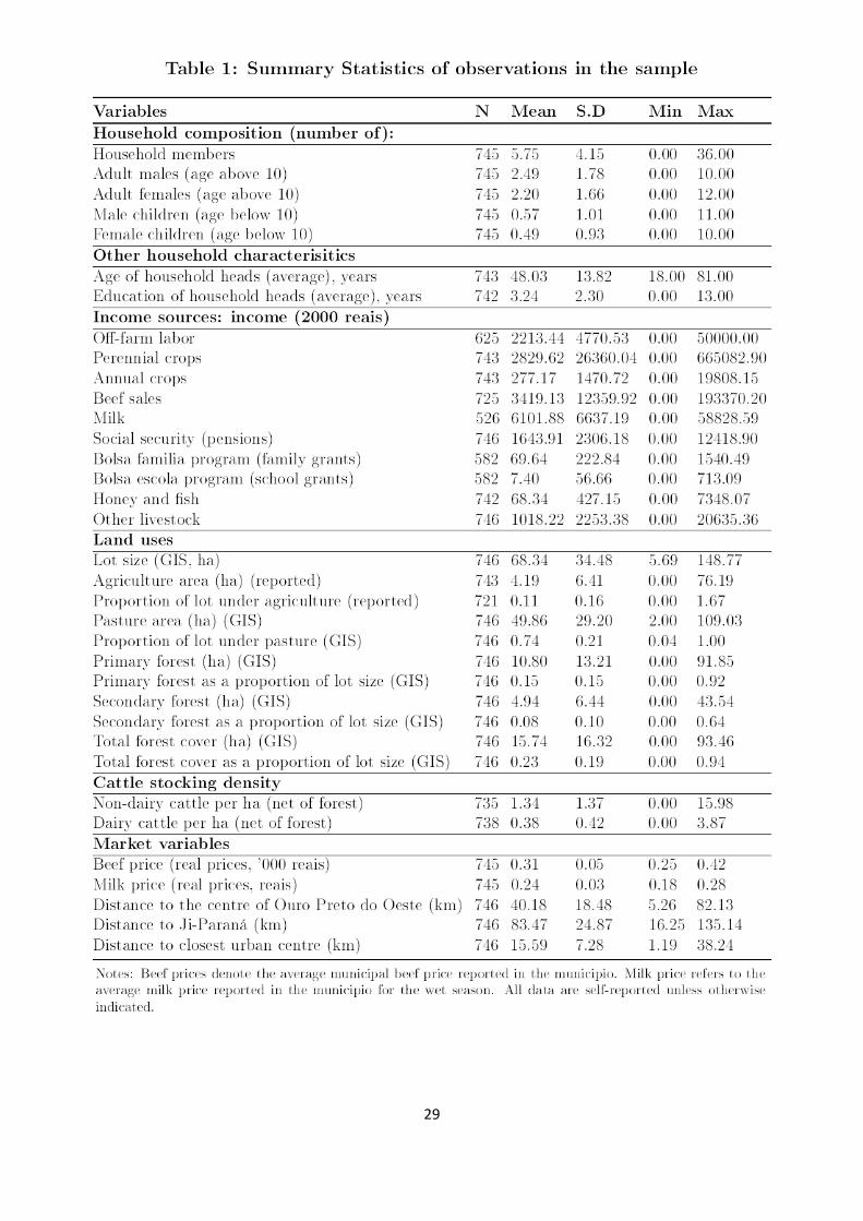
29

30

31

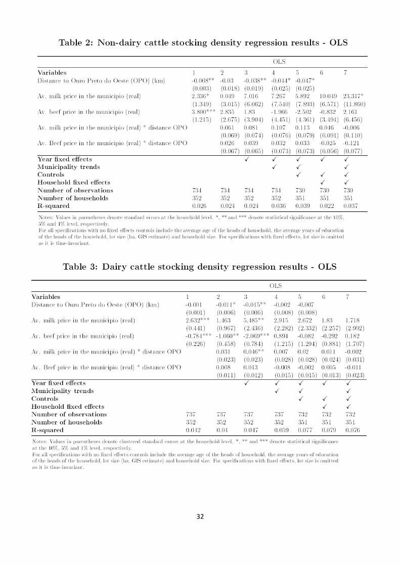
32

33

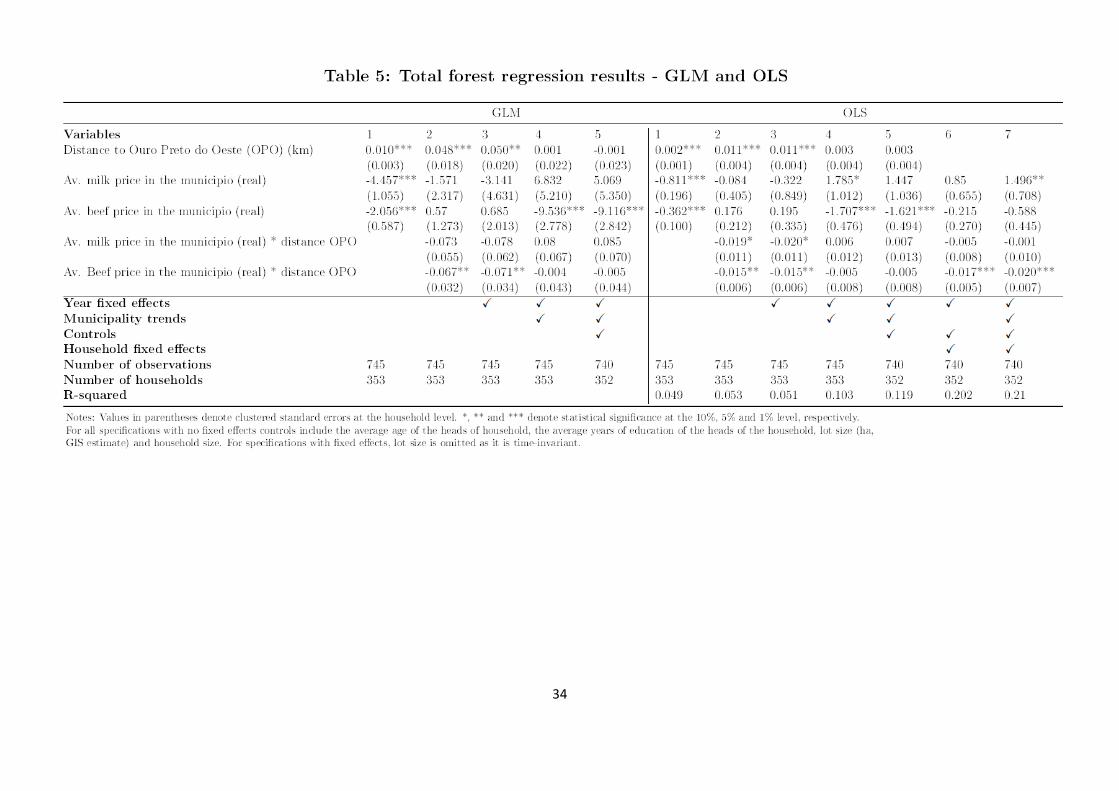
34

35

36

37

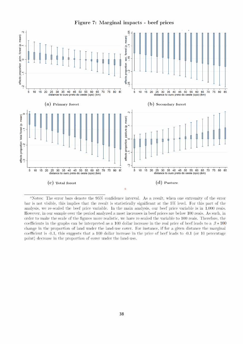
38

39

40

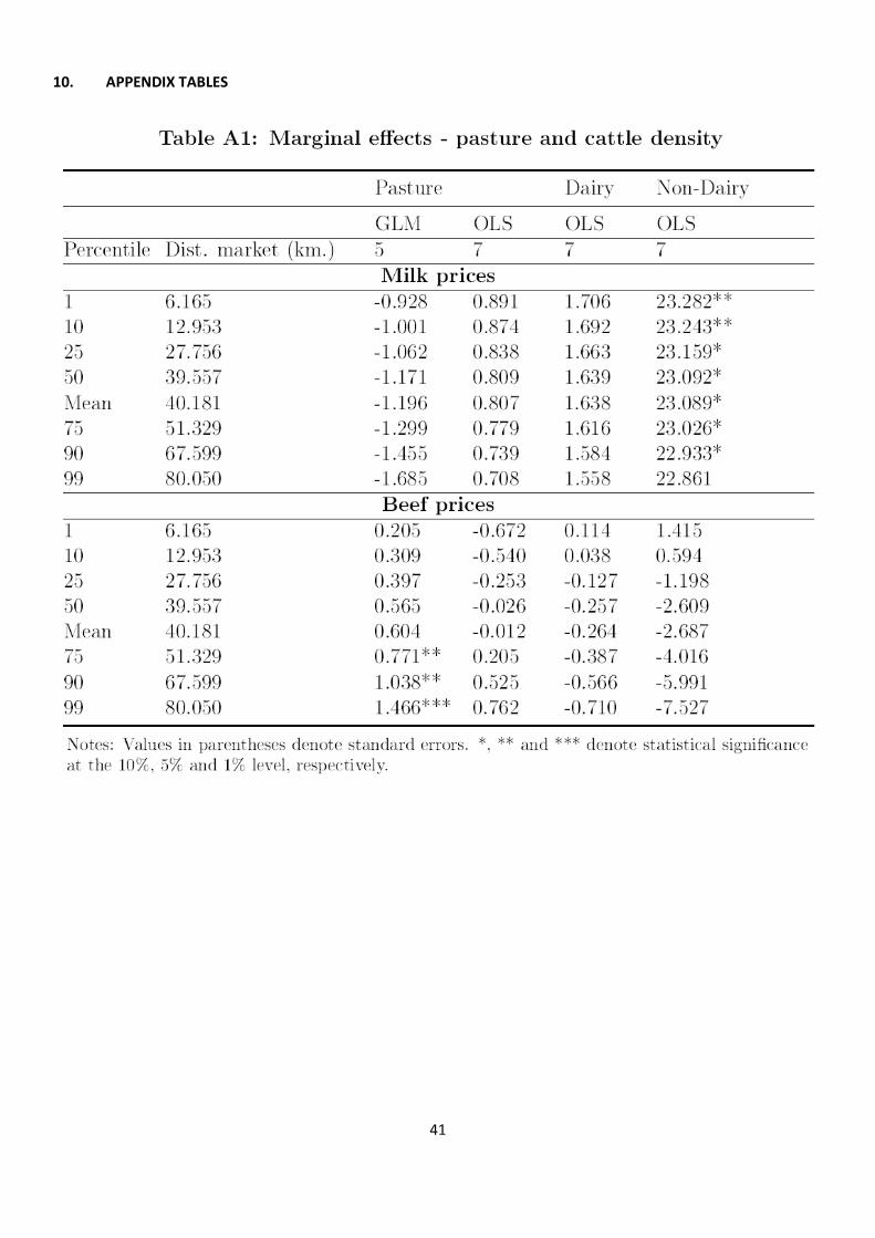
41

10. APPENDIX TABLES

42

43

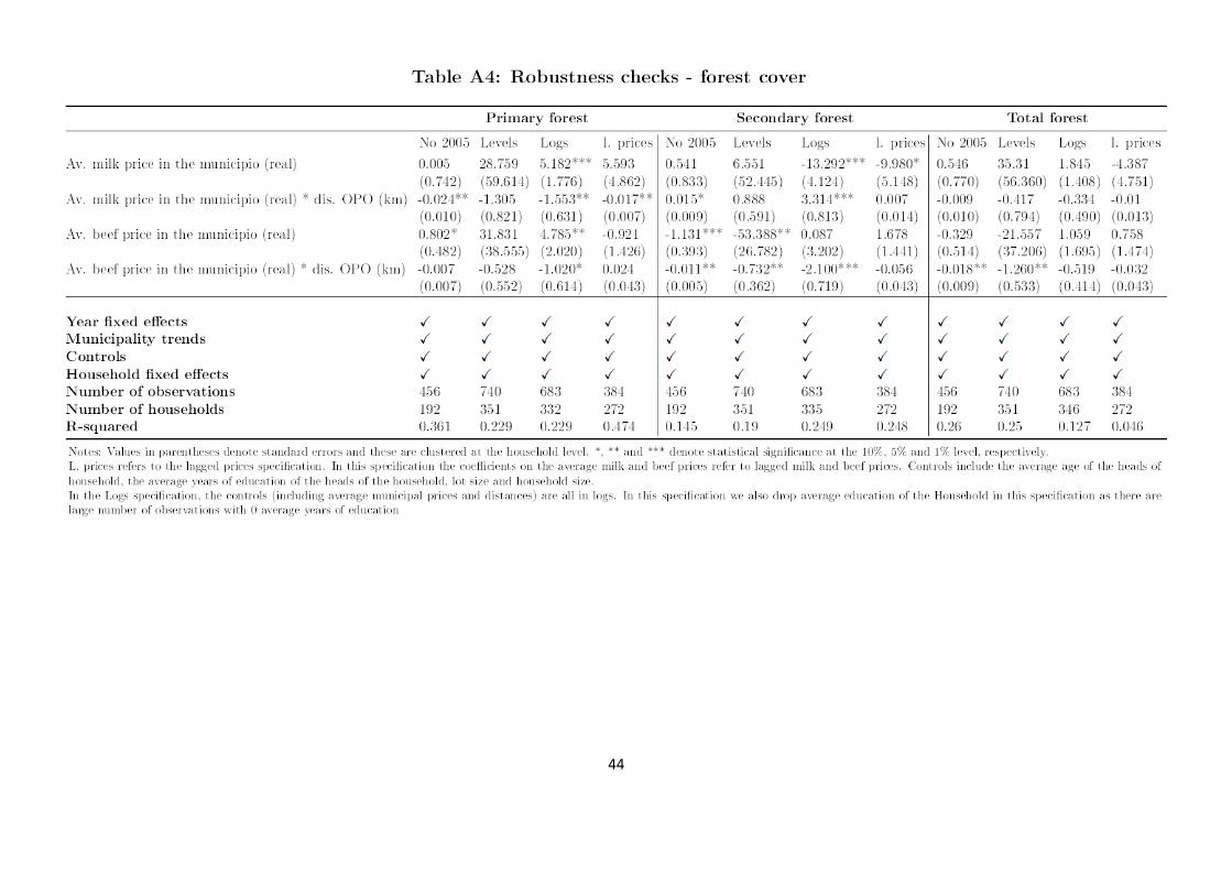
44

45

46

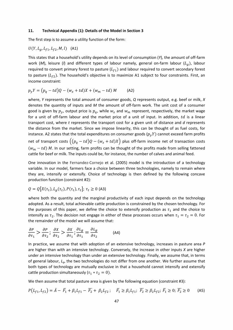
47

11. Technical Appendix (1): Details of the Model in Section 3

The first step is to assume a utility function of the form:

�(, ��, ���, ���, , �) (A1)

This states that a household’s utility depends on its level of consumption (Y), the amount of off-farm

work (M), leisure (l) and different types of labour namely, general on-farm labour (��), labour

required to convert primary forest to pasture (���) and labour required to convert secondary forest

to pasture (���). The household’s objective is to maximize A1 subject to four constraints. First, an

income constraint:

� = � � − ���� − (�� + ��)� + (�� − ��) (A2)

where, Y represents the total amount of consumer goods, Q represents output, e.g. beef or milk, X

denotes the quantity of inputs and M the amount of off-farm work. The unit cost of a consumer

good is given by �, output price is �, while �� and �� represent, respectively, the market wage

for a unit of off-farm labour and the market price of a unit of input. In addition, �� is a linear

transport cost, where t represents the transport cost for a given unit of distance and d represents

the distance from the market. Since we impose linearity, this can be thought of as fuel costs, for

instance. A2 states that the total expenditures on consumer goods ( �) cannot exceed farm profits

net of transport costs /� � − ���� − (�� + ��)�4 plus off-farm income net of transaction costs

(�� − ��). In our setting, farm profits can be thought of the profits made from selling fattened

cattle for beef or milk. The inputs could be, for instance, the number of calves and animal feed.

One innovation in the Fernandez-Cornejo et al. (2005) model is the introduction of a technology

variable. In our model, farmers face a choice between three technologies, namely to remain where

they are, intensify or extensify. Choice of technology is then defined by the following concave

production function (constraint #2):

� = ���(��), ��(��), J(��), ���;�� ≥ 0 (A3)

where both the quantity and the marginal productivity of each input depends on the technology

adopted. As a result, total achievable cattle production is constrained by the chosen technology. For

the purposes of this paper, we define the choice to extensify production as �� and the choice to

intensify as ��. The decision not engage in either of these processes occurs when �� = �� = 0. For

the remainder of the model we will assume that:

(9(*+ > (9

(*2 ; (,(*2 > (,

(*+ ; (03(*+ = (03(*2 (A4)

In practice, we assume that with adoption of an extensive technology, increases in pasture area P

are higher than with an intensive technology. Conversely, the increase in other inputs X are higher

under an intensive technology than under an extensive technology. Finally, we assume that, in terms

of general labour, Lg, the two technologies do not differ from one another. We further assume that

both types of technology are mutually exclusive in that a household cannot intensify and extensify

cattle production simultaneously (�� ∗ �� = 0).

We then assume that total pasture area is given by the following equation (constraint #3):

J����, ���� = K̅ − M�N + ;���� − M�OOO + ;����; M�N ≥ ;����; M�OOO ≥ ;����; M�N ≥ 0;M�OOO ≥ 0 (A5)

48

where K̅ represents the total (exogenous) lot area, and M�N and M�OOO denote the total exogenous initial

amount of primary and secondary forest on the lot, respectively. Forest can be converted into new

pasture land. Primary forest can be cleared with labour ��� and each unit of this type of labour leads

to a ;� increase in pasture area. Similarly, for secondary forest, an additional unit of ��� leads to a ;�

increase in the pasture area. We further assume that ;� > ;�. In other words, we assume that it is

cheaper to clear secondary forest than primary forest in that for a given input of labour a larger

amount of land can be converted into pasture from secondary than primary forest.

The final constraint is a time constraint where it is assumed that:

! = �� + ��� + ��� + + �; ≥ 0; ��� ≥ 0; ��� ≥ 0; �� > 0; � ≥ 0 (A6)

Thus, the total time of the household is allocated between a strictly positive amount of general

labour (��), a non-negative amount of land clearing labour (���, ���), a non-negative amount of off-

farm labour () and a non-negative amount of leisure (l).

Plugging in the technology constraint and using the fact that pasture can be expressed as a function

of labour, we can rewrite the first constraint (A3):

� = � � − ������(��), ��(��), ���(��), ���(��), �� , � − (�� + ��)� + (�� − ��)(A7) We now write the Lagrangian as follows:

� = ��, ��, ���, ���, , �� + &�� � − ������(��), ��(��), ���(��), ���(��), �� , � − (�� + ��)� +(�� − ��) − R� − '�! − �� − ��� − ��� − − �� (A8)

Take the first order derivatives:25

S�S = S�S − & R = 0(K9)

S�S� = S�S� − ' = 0(K10)

S�S� = & V� � − ��� S�S� − ��W = 0(K11)

S�S��� = & V� � − ��� S�SJ ;�W − ' ≤ 0;M�Nβ� ≥ ��� ≥ 0, ��� Y& V� � − ��� S�SJ ;�W − 'Z = 0;(K12)

S�S��� = & V� � − ��� S�SJ ;�W − ' ≤ 0;M�OOOβ� ≥ ��� ≥ 0, ��� Y& V� � − ��� S�SJ ;�W − 'Z = 0;(K13)

Note: ()(01+ = ()

(9(9

(01+ ; takethederivativeof (9(01+ and we have ;�. Also:

()(012 = ()

(9(9

(012 ; takethederivativeof (9(012 and we have ;�.

49

Note that, since ;� < ;�, we have that if & i� � − ��� ()(9 ;�j − ' < 0, then by definition,

& i� � − ��� ()(9 ;�j − ' < 0 will also hold. This implies two things. If the marginal productive effects

of converting secondary forest into pasture do not compensate the hours worked by the household,

then the household will not convert primary forest. In other words, if the optimal level of labour for

conversion from secondary forest to pasture is 0 (i.e. ��� = 0), then the same will hold for ���. The

intuition behind this is simple. Since it is cheaper to convert secondary than primary forest, the

household will only convert primary forest if there is no secondary forest remaining or if there is

insufficient secondary to allow for the total desired pasture area. This suggests that we are likely to

see more pronounced effects on reduction of secondary forest in contrast to primary forest.

S�S�� = & k� � − ��� S�S��l − ' = 0; �� > 0(K14)

S�S = &n�� − ��o − ' = 0; ≥ 0, (&�� − ') = 0(K15)

Finally:

S�S�� = & k� � − ��� kS�S� S�S�� + S�S��S��S�� + S�SJ SJS���

S���S�� + S�SJ SJS���S���S�� + S�S��l − (�� + ��) S�S�� l

− ' S���S�� − ' S���S�� − ' S��S�� ≤ 0; �� ≥ 0, �� S�S�� = 0(A16)

Equation (A16) states that a household will adopt technology t if the benefits of adopting this

technology exceed the costs of adoption. As such, if this equation is a strict inequality for t=1,2 , no

technology will be adopted. Looking at the technology adoption decision separately, technologies 1

and 2 are adopted if:

� � − ��� S�S�� ≥ (�� + ��) S�S�� + '& rS���S�� + S���S�� + S��S�� s(K17)

� � − ��� S�S�� ≥ (�� + ��) S�S�� + '& rS���S�� + S���S�� + S��S�� s(K18) Note from the first-order conditions (A9, A10 and A15) that, for non-zero quantities of off-farm

labour we have:

'& = �� − �� = k� � − ��� S�S��l(K17)

As a result, if we assume that ()

(03 is the same under �� and ��, we have that, the furthest away the

households are from the market, the lowest -. but the highest input costs (�� + ��). This result

implies that, if extensification and intensification affect revenues in the same way, the further a

household is from the market the more likely it is to extensify. Suppose for simplicity that

i ()(*+j = i ()

(*2j, i.e. a one-unit increase in adoption of a more intensive technology leads to the same

output increase as a one-unit output increase from adopting an extensive technology. The

household will adopt a more extensive production system if:

50

(�� + ��) S�S�� + '& S���S�� + '& S���S�� + '& S��S�� ≤ (�� + ��) S�S�� + '& S���S�� + '& S���S�� + '& S��S�� (K18)

We can rearrange this such that:

'& rS���S�� + S���S�� + S��S�� − S���S�� − S���S�� − S��S��s ≤ (�� + ��) Y S�S�� − S�S��Z(K19)

Since we assumed at the beginning that (03(*+ = (03(*2 these terms disappear. And, since

-. is decreasing

in distance to market and (�� + ��) is increasing in distance to market, then the further away the

household is from the market, the more likely it is to adopt an extensive technology, given that the

opportunity costs of working off-farm are lower (due to higher transportation costs), the costs of

purchasing inputs are higher (again due to higher transportation costs), and extensive production

systems are assumed to be more labour-intensive as opposed to more intensive in other inputs.

12. Technical Appendix (2): Adding a PES to the Model in Section 3

First, we assume that for each additional unit of forest, primary or secondary, in the lot, the

household is offered a subsidy or PES of s to keep the forest standing rather than convert it to

pasture. Our set of constraints is then augmented with a fifth constraint in the form of a

deforestation function:

M� = M�N − ;����; M� = M�OOO − ;���� (A20 )

The full income constraint can be rewritten as:

� = � � − ������(��), ��(��), ���(��), ���(��), �� , � − (�� + ��)� + (�� − ��) + E(M�N −;���� + M�OOO − ;����) (A21)

The resulting Lagrangian is:

� = ��, ��, ���, ���, , ��+ &�� � − ������(��), ��(��), ���(��), ���(��), �� , � − (�� + ��)� + (�� − ��)+ E(M�N − ;���� + M�OOO − ;����) − R� − '�! − �� − ��� − ��� − − ��(K22)

The first-order conditions are similar to those derived in Technical Appendix (2), with the exception

of:

S�S��� = & V� � − ��� S�SJ ;�W − E;� − ' ≤ 0;M�Nβ� ≥ ��� ≥ 0, ��� Y& V� � − ��� S�SJ ;�W − E;� − 'Z= 0;(K23)

S�S��� = & V� � − ��� S�SJ ;�W − E;� − ' ≤ 0;M�OOOβ� ≥ ��� ≥ 0, ��� Y& V� � − ��� S�SJ ;�W − E;� − 'Z

= 0;(K24)

As before, since ;� < ;�, we have that if & i� � − ��� ()(9 ;�j − E;� − ' < 0, then by definition,

& i� � − ��� ()(9 ;�j − E;� − ' < 0 will also hold. For a non-zero level of conversion of forest

(primary or secondary), a household with the option of participating in a PES scheme would compare

the marginal benefits of converting forest to pasture against the marginal cost of household time

required to clear forest plus income from the PES scheme.

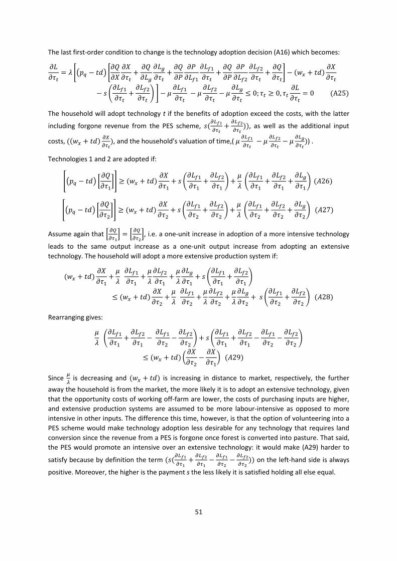
51

The last first-order condition to change is the technology adoption decision (A16) which becomes:

S�S�� = & k� � − ��� kS�S� S�S�� + S�S��S��S�� + S�SJ SJS���

S���S�� + S�SJ SJS���S���S�� + S�S��l − (�� + ��) S�S��

− E rS���S�� + S���S�� sl − ' S���S�� − ' S���S�� − ' S��S�� ≤ 0; �� ≥ 0, �� S�S�� = 0(A25)

The household will adopt technology t if the benefits of adoption exceed the costs, with the latter

including forgone revenue from the PES scheme, E((01+(*u + (012(*u )), as well as the additional input

costs, ((�� + ��) (,(*u), and the household’s valuation of time,( ' (01+(*u − ' (012(*u − ' (03(*u )) .

Technologies 1 and 2 are adopted if:

v� � − ��� V S�S��Ww ≥ (�� + ��) S�S�� + E rS���S�� + S���S�� s + '& rS���S�� + S���S�� + S��S�� s(K26)

v� � − ��� V S�S��Ww ≥ (�� + ��) S�S�� + E rS���S�� + S���S�� s + '& rS���S�� + S���S�� + S��S�� s(K27) Assume again that i ()

(*+j = i ()(*2j, i.e. a one-unit increase in adoption of a more intensive technology

leads to the same output increase as a one-unit output increase from adopting an extensive

technology. The household will adopt a more extensive production system if:

(�� + ��) S�S�� + '& S���S�� + '& S���S�� + '& S��S�� + E rS���S�� + S���S�� s≤ (�� + ��) S�S�� + '& S���S�� + '& S���S�� + '& S��S�� + E rS���S�� + S���S�� s(K28)

Rearranging gives:

'& rS���S�� + S���S�� − S���S�� − S���S�� s + E rS���S�� + S���S�� − S���S�� − S���S�� s≤ (�� + ��) Y S�S�� − S�S��Z(K29)

Since -. is decreasing and (�� + ��) is increasing in distance to market, respectively, the further

away the household is from the market, the more likely it is to adopt an extensive technology, given

that the opportunity costs of working off-farm are lower, the costs of purchasing inputs are higher,

and extensive production systems are assumed to be more labour-intensive as opposed to more

intensive in other inputs. The difference this time, however, is that the option of volunteering into a

PES scheme would make technology adoption less desirable for any technology that requires land

conversion since the revenue from a PES is forgone once forest is converted into pasture. That said,

the PES would promote an intensive over an extensive technology: it would make (A29) harder to

satisfy because by definition the term (E((01+(*+ + (012(*+ − (01+(*2 − (012(*2 )) on the left-hand side is always

positive. Moreover, the higher is the payment s the less likely it is satisfied holding all else equal.

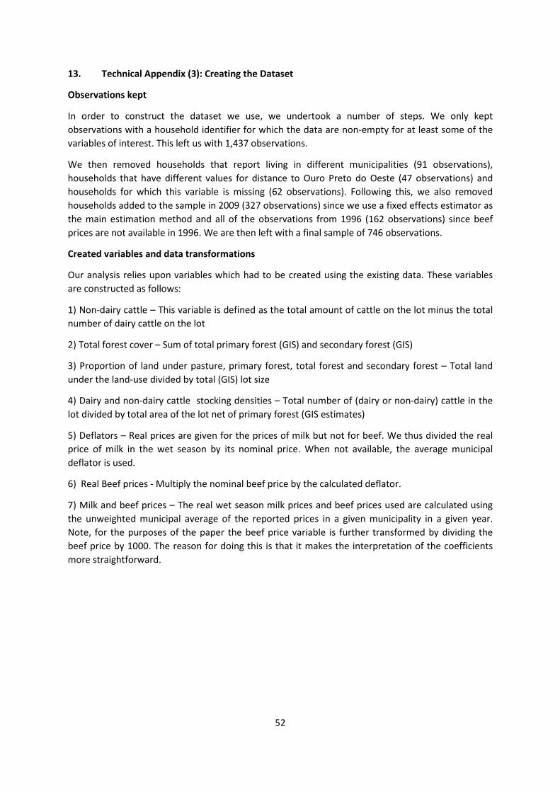
52

13. Technical Appendix (3): Creating the Dataset

Observations kept

In order to construct the dataset we use, we undertook a number of steps. We only kept

observations with a household identifier for which the data are non-empty for at least some of the

variables of interest. This left us with 1,437 observations.

We then removed households that report living in different municipalities (91 observations),

households that have different values for distance to Ouro Preto do Oeste (47 observations) and

households for which this variable is missing (62 observations). Following this, we also removed

households added to the sample in 2009 (327 observations) since we use a fixed effects estimator as

the main estimation method and all of the observations from 1996 (162 observations) since beef

prices are not available in 1996. We are then left with a final sample of 746 observations.

Created variables and data transformations

Our analysis relies upon variables which had to be created using the existing data. These variables

are constructed as follows:

1) Non-dairy cattle – This variable is defined as the total amount of cattle on the lot minus the total

number of dairy cattle on the lot

2) Total forest cover – Sum of total primary forest (GIS) and secondary forest (GIS)

3) Proportion of land under pasture, primary forest, total forest and secondary forest – Total land

under the land-use divided by total (GIS) lot size

4) Dairy and non-dairy cattle stocking densities – Total number of (dairy or non-dairy) cattle in the

lot divided by total area of the lot net of primary forest (GIS estimates)

5) Deflators – Real prices are given for the prices of milk but not for beef. We thus divided the real

price of milk in the wet season by its nominal price. When not available, the average municipal

deflator is used.

6) Real Beef prices - Multiply the nominal beef price by the calculated deflator.

7) Milk and beef prices – The real wet season milk prices and beef prices used are calculated using

the unweighted municipal average of the reported prices in a given municipality in a given year.

Note, for the purposes of the paper the beef price variable is further transformed by dividing the

beef price by 1000. The reason for doing this is that it makes the interpretation of the coefficients

more straightforward.