Embed Size (px)
Citation preview

Washington Road Surface
Erosion Model
Prepared for: State of Washington
Department of Natural Resources
By:
Kathy Dubé Walt Megahan
Marc McCalmon
February 20, 2004

Page i February 20, 2004
WASHINGTON ROAD SURFACE EROSION MODEL (WARSEM) MANUAL
Contents Overview......................................................................................................................................... 1 Chapter 1 Introduction ................................................................................................................... 3 Chapter 2 Use of Road Surface Erosion Model............................................................................. 6
2.1 Access Database Applications ............................................................................................. 8 2.2 SEDMODL2 Applications................................................................................................... 8
Chapter 3 Project Set Up.............................................................................................................. 10 3.1 Examples............................................................................................................................ 10
RMAPs – Tracking effects of BMPs on Small Parcels ........................................................ 10 Scenario Playing – Which BMPs Will Be Most Cost-Effective?......................................... 10 Watershed Analysis and Sediment Budgeting...................................................................... 11 FFR Performance Metrics (Monitoring)............................................................................... 11
Chapter 4 Input Data Requirements and Field Protocols............................................................. 12 4.1 Pre-field Data Collection and Preparation ......................................................................... 13 4.2 Field Work ......................................................................................................................... 14
Road Inventory Methods....................................................................................................... 15 Header Information............................................................................................................... 19 Road Segment Numbers, Groups, and Lengths .................................................................... 19 Year Road Built .................................................................................................................... 20 Erosion Rating ...................................................................................................................... 20 Road Slope Class .................................................................................................................. 21 Road Configuration............................................................................................................... 21 Surfacing ............................................................................................................................... 22 Average Tread Width............................................................................................................ 23 Traffic Use ............................................................................................................................ 23 Cutslope Cover Density ........................................................................................................ 24 Cutslope Average Height...................................................................................................... 24 Ditch Width........................................................................................................................... 25 Ditch Delivery....................................................................................................................... 25 Ditch Condition..................................................................................................................... 26 BMPs..................................................................................................................................... 26 Problem Area/Comments...................................................................................................... 26 Class...................................................................................................................................... 26 Position ................................................................................................................................. 26 Base Map .............................................................................................................................. 26
Chapter 5 Access Application...................................................................................................... 28 5.1 Loading the Application .................................................................................................... 28 5.2 Starting the Application ..................................................................................................... 29
Use a Wizard......................................................................................................................... 30 Start From Scratch ................................................................................................................ 32 Open an Existing Project ...................................................................................................... 33
5.3 Importing Data ................................................................................................................... 34 5.4 Inputting and Editing Road Data ....................................................................................... 36
Selecting Default Values....................................................................................................... 36

Washington Road Surface Erosion Model
Entering and Editing Data..................................................................................................... 38 Editing Existing Data............................................................................................................ 40
5.5 Applying BMPs and Creating Custom BMPs ................................................................... 40 Custom BMPs ....................................................................................................................... 41
5.6 Using Model Menus........................................................................................................... 43 File ........................................................................................................................................ 43 Selection................................................................................................................................ 43 Updates ................................................................................................................................. 47 Query..................................................................................................................................... 49 Reports .................................................................................................................................. 50 Options.................................................................................................................................. 50
5.7 Running the Model to Calculate Surface Erosion.............................................................. 50 5.8 Output Reports ................................................................................................................... 52 5.9 Exporting records............................................................................................................... 53 5.10 File management.............................................................................................................. 54
Chapter 6 Interpreting Model Results.......................................................................................... 55 List of Figures
Figure 1. Components of a Road Prism. ........................................................................................ 4 Figure 2. Components of a Road Prism and Field Measured Parameters ................................... 18 Figure 3. Generalized Runoff Flow Paths for Different Road Drainage Configurations. ........... 18 Figure 4. Example Road Segments.............................................................................................. 19 Figure 5. Example of a road segment draining to another segment............................................. 20 Figure 6. Outsloped road.............................................................................................................. 21 Figure 7. Road with two ditches and wheel tracks. ..................................................................... 22 Figure 8. Crowned road with 2 ditches........................................................................................ 25 Figure 9. Sample Field Map and Data Sheet ............................................................................... 27 List of Tables
Table 1. Application Matrix........................................................................................................... 7 Table 2. Data needed for each model level.................................................................................. 12 Table 3. Field and Data Entry Form ............................................................................................ 16 Table 4. Surface Erosion Road Survey Field/Data Entry Form Instructions............................... 17 Table 5. WARSEM Modeling of Different Road Configurations. .............................................. 21 Table 6. Traffic Use Categories. .................................................................................................. 24 Table 7. Use of Selection Menu Choices..................................................................................... 44 List of Appendices Appendix A. Technical Documentation Appendix B. Field Protocols/Data Sheets Appendix C. Best Management Practices (BMPs) Appendix D. Field Testing Results Appendix E. Data Import Format Requirements
Page ii February 20, 2004

Washington Road Surface Erosion Model
List of Preparers
Kathy Vanderwal Dubé, Watershed GeoDynamics Walter F. Megahan Marc McCalmon, Terra GIS Solutions This application and manual were funded by the Washington Department of Natural Resources as part of Contract No. PSC-02-257.
Acknowledgements The authors wish to gratefully acknowledge all the field testers who so generously gave their time to try out the field methods during those chilly February days and to provide feedback on improvements to the field protocols. Field testers included Brian Ballard, Dan Christensen, Jeffrey Clark, Jerry Clarke, Julie Dieu, Terry Domning, Harry Elliott, Abby H, Bob Layton, Dave Luzi, Donelle Mahan, Bob Marx, Matt McLaughlin, Danny O’Sullivan, Bob Palmquist, Luke Rogers, Kathy Smayda, Dan Thomas, and Todd Zackey. Thanks also to the landowners who provided and arranged for access to their road systems for the field testing, including Rayonier, Washington Department of Natural Resources, and Weyerhaeuser. In addition, many thanks to the members of the UPSAG committee and all others who reviewed various drafts of the manual and tested the beta version of the Access model. Your comments and thoughts are appreciated and helped to improve the manual and model. Reviewers included Robert Bass, Jeffrey Clark, Drew Coe, Julie Dieu, Milt Holter, Mark Hunter, George Ice, Leslie Lingley, Dave Luzi, Bob Palmquist, Dave Parks, Mary Raines, Luke Rogers, Nancy Sturhan, and Laura Vaugeois.
Page iii February 20, 2004

Washington Road Surface Erosion Model
Page iv February 20, 2004

Page 1 February 20, 2004
WASHINGTON ROAD SURFACE EROSION MODEL MANUAL
Overview
The Washington Road Surface Erosion Model is a tool that allows users to calculate average annual road surface erosion and sediment delivery to channels in a standardized manner. The model is intended for use on forest roads in Washington State, and can be applied on a variety of scales, ranging from a single road segment to all roads within a watershed or road planning unit. The model is designed to interface with a GIS system if such spatial data are available. The analysis can be carried out at 4 different levels, depending upon the purpose of the analysis and the level of detail of data available for the roads:
Level 1 – Screening. Assessment tool for determining relative sediment contributions from roads using little site-specific information for the roads. Useful for screening road system to prioritize field work.
Level 2 – Planning-level Assessment. Assessment of erosion and delivery appropriate for road maintenance planning or sediment budgeting using minimal site-specific information for the roads
Level 3 – Detailed Assessment and Scenario Playing. Detailed assessment of modeled erosion/delivery using field-verified data on each road segment. Ability to determine reduction in sediment delivery resulting from applying potential road maintenance practices or Best Management Practices (BMPs) to road segments (scenario playing).
Level 4 – Site/Segment Level Monitoring. Ability to track changes in road segment attributes and modeled erosion/delivery resulting from road maintenance or BMPs through time. Used to document and monitor reduction in road surface erosion resulting from Road Maintenance and Abandonment Plans (RMAPs) and to compute Forest and Fish Rules (FFR) performance metrics. Can be used for watershed-scale evaluations.
Data for the road system or segments is entered into a data management application (Access) for calculation of the modeled annual road surface erosion and sediment delivery to waterways. Data can be entered and edited within the Access application, or can be imported from another source, such as a GIS data file, Excel file, or SEDMODL2 run (SEDMODL2 is a GIS program that calculates road surface erosion). The application stores road information in a database and computes the amount of modeled road surface erosion delivered to streams. Road records can be updated as new information becomes available from field inventories or improvements to the roads. The model produces output reports detailing input parameters and the results of erosion and sediment delivery calculations. Model output can also be exported to GIS or a comma delimited file for further analysis by the user.
This Manual is organized into six chapters. Chapter 1 provides an overview of road surface erosion processes. Chapter 2 describes the four different model levels in greater detail and specifies the data required for each level. Chapter 3 provides recommendations for setting up a new project and organizing data efficiently. Chapter 4 lists the data required to run the model, describes field inventory protocols, and explains how to measure the characteristics of roads in

Washington Road Surface Erosion Model
the field. Chapter 5 includes instructions on how to use the Access Application, from setting up the program on your computer to the data entry screens and output reports. Chapter 6 describes how to interpret model results. The appendices provide technical information on how the road model works, how the equations and factors that are used to compute road erosion were derived, sample field forms that can be copied and used for field inventories of roads, more detailed information on the application of BMPs, and the results of the field testing and repeatability of field protocols.
Page 2 February 20, 2004

Washington Road Surface Erosion Model
Chapter 1 Introduction
Roads play an important role in our society, providing vital links for transportation of people and materials quickly and efficiently. There are hundreds of thousands of miles of roads in Washington State. Many of these roads are unpaved forest roads, used to access lands managed primarily for timber harvest. Forest roads provide many useful functions such as allowing timber products to be transported efficiently to mills, providing access for recreationalists, hunters, and fishermen, and even giving wildlife easy travel corridors. However, roads can also have deleterious effects. The construction and use of roads can be a major source of sediment in forested basins. Sediment that reaches streams, wetlands, or lakes can have an impact on water quality, fish, and other aquatic life.
Increased sediment from roads can result from three major erosion processes: surface erosion, gullying, or mass wasting (Landslides). Each of these processes can be important. However, surface erosion occurs on all roads whereas gullies and landslides are limited to specific locations on steep slopes and/or unique geologic and soil conditions. Surface erosion produces fine-grained sediment (sand, silt, clay) that can harm fish and other aquatic organisms if it enters streams. The methods described in this manual are designed to address the issue of surface erosion from roads.
Surface erosion is defined as the detachment of individual soil particles by a force such as raindrop impact, overland flow of water, wind, or gravity. Detachment of soil particles depends not only on the amount of external force applied but also on how well the soil particles tend to resist separation. This latter factor is an inherent soil property termed soil erodibility and is strongly influenced by the texture (grain size) of the exposed soil. Generally, gravelly or cohesive soils are not as easily eroded as sandy or silty soils. Erosion is usually not an issue under Washington Forest Practice regulations unless the sediment is transported to streams or waterbodies.
In the majority of forested basins, a thick layer of duff protects the soil from surface erosion, and most rainfall and snowmelt infiltrates into the soil. However, construction of a forest road in mountainous terrain can lead to high rates of surface erosion due to: 1) removal of all vegetative cover and surface protection; 2) the construction of cut and fill slopes that are steeper than the original hillslope in order to obtain a relatively level driving surface; 3) greatly increased potential for overland water flow due to soil compaction and concentration of runoff; and 4) interception of groundwater by the cut slope. The latter factor is the primary cause of sediment transport from the roadway. Compacted road surfaces, long lengths of roads without cross drains, areas with heavy rainfall, and soils prone to gully formation are more likely to result in transport of eroded sediment off the road prism. Transport of sediment to a stream is most likely to occur when the road is close to a stream, there is a steep slope between the road and the stream, and there are few obstructions to slow down or trap the sediment. Sediment is likely to be trapped (deposited) before it enters a stream if it is produced from roads far from a stream, or from roads with a vegetative buffer or topographic low between the road and the stream.
In Washington State, the Department of Natural Resources (WDNR) has implemented a Road Maintenance and Abandonment Plan (RMAP) program for forest roads under WDNR jurisdiction. One of the goals of the RMAP program is to ensure forest roads are maintained in a way that helps protect fish and aquatic organisms from the harmful effects of sediment produced
Page 3 February 20, 2004

Washington Road Surface Erosion Model
from the road system. RMAPs are designed to improve many aspects of the road network by reducing the likelihood of road landslides, culvert plugging, road surface erosion, and fish passage barriers. The Washington Road Surface Erosion Model has been designed based on the surface erosion assessment in the Watershed Analysis Procedure to support a number of assessment and monitoring needs related to roads. The primary motivation for the revision is for use as a monitoring tool, but the model can also help landowners estimate the amount of sediment supplied from the surface erosion component of their road system and the relative effectiveness of different measures to reduce road surface erosion in order to meet RMAP goals.
The Washington Road Surface Erosion Model produces estimates of the long-term average amount of sediment that could be expected from a road with similar characteristics. Why the long-term average? We know from measurements of road surface erosion that the amount of sediment delivered to streams from roads is influenced by a number of factors including the physical setting, the proximity of the road to a stream, the condition of the road, the amount and intensity of rainfall and the amount and type of traffic. The actual quantity of sediment eroded from a particular road segment varies greatly from year to year as a result of differences in precipitation, traffic, and maintenance activities. Our ability to measure or predict all of these factors precisely at each location we would like to model is limited. However, it is useful to predict where roads have the potential to produce relatively high amounts of sediment based on our current understanding of road erosion processes and typical conditions of each road segment. The model output, in average annual tons of sediment per year, allows road managers to identify road segments that are most likely to produce larger amounts of sediment, and to determine the relative sediment savings from a variety of management practices.
The Washington Road Surface Erosion Model is a database program that allows the user to enter information about a road system and to calculate the estimated average annual amount of sediment delivered to streams from the road(s). The user can enter information about a single road segment, several roads, or all the roads in an area or watershed. The program has the ability to keep track of improvements to the road system through time, and to calculate the resulting changes in surface erosion. A brief description of how the model calculates erosion and delivery follows; complete details of the equations and factors used are included in Appendix A (Technical Documentation).
Figure 1. Components of a Road Prism. There are four distinct parts of a normal road prism constructed on a hillslope: the cutslope, fillslope, ditch, and tread (Figure 1). Some roads may not have a ditch, cutslope or fillslope, or may have two cutslopes or ditches. Examples of roads without one or more of these components are roads on flat ground, full bench roads, outsloped roads, or through cut roads.
Fillslope
Cutslope
Tread
Ditch
Page 4 February 20, 2004

Washington Road Surface Erosion Model
On a newly constructed road, each of these parts of the road prism are typically exposed and subject to erosion. Over time, the cutslope and fillslope revegetate and erosion from these sources is reduced. In most established road networks, the fillslopes have nearly 100 percent vegetative cover, and do not deliver to streams. However, the road tread and ditch, and to a lesser extent the cutslope, continue to be sediment sources as long as the road is in use. Research has shown that the most important factors determining how much sediment is produced from the road tread are how much the road is used, and the amount and type of road surfacing. The amount of cover on the cutslope, armoring in the ditch, and whether or not these surfaces have been re-graded recently, affect erosion from these components. In addition to these factors, the configuration of the road drainage system, particularly whether or not road drainage reaches the stream network, determines if sediment produced from roads has the potential to affect aquatic resources.
The Washington Road Surface Erosion Model calculates the average annual amount of road surface erosion that is delivered to a stream from each road segment entered into the model. The erosion calculations are based on a set of empirical relationships that have been developed from research on road erosion. When evaluating model results, keep in mind that the output, reported in average tons per year, is an estimate, not a precise value. Comparison of the relative amount of sediment produced from different segments or comparison of results from a single segment with different BMPs applied is an appropriate use of the model output. It is not wise to expect that the absolute values predicted are necessarily accurate for any given road segment in a given year.
The model uses a base erosion rate that is dependent upon the type of soil (geology) the road is built on. The base erosion rate is multiplied by a series of factors that either increase or decrease the amount of erosion, depending upon the characteristics of the road tread, ditch, and cutslope, and how much of the eroded sediment is predicted to reach a stream.
The model uses the following formulas to calculate road surface erosion:
Total Sediment Delivered to a Stream from each Road Segment (in tons/year) = (Tread & Ditch Sediment + Cutslope Sediment) x Road Age Factor
Tread & Ditch = Geologic Erosion Factor x Tread Surfacing Factor x Traffic Factor x Segment Length x Road (Tread + Ditch) Width x Road Gradient Factor x Rainfall Factor x Delivery Factor
Cutslope = Geologic Erosion Factor x Cutslope Cover Factor x Segment Length x Cutslope Height x Rainfall Factor x Delivery Factor
The model determines the value for each factor in the equations based on information the user enters for individual road segments. Information on how to select the appropriate values for road characteristics is included in Chapter 4 (Field Protocols). Details of the numerical values for each factor and how they were derived are included in Appendix A (Technical Documentation).
Page 5 February 20, 2004

Washington Road Surface Erosion Model
Chapter 2 Use of Road Surface Erosion Model
The Washington Road Surface Erosion Model was designed to be flexible enough to be run for a wide variety of road situations and with different levels of detail on the road system. A user can enter only basic information about a road segment (length, location, and delivery type) and use default values for all other variables. The calculated amount of erosion using this limited data would be a very rough estimate, and useful only for screening or general comparison purposes. On the other hand, a user can enter site-specific information about every portion of the road prism based on a field visit to the road segment. The result of this calculation will be much more precise, and can be used to track changes to road erosion through time, to compare erosion from different road segments or groups of segments, or to compare the effects of various road management schemes on sediment production from surface erosion.
It is important to remember that the estimated erosion produced from model calculations are estimated long-term average amounts of sediment that could be expected from a road with similar conditions. The actual amounts of sediment produced from a specific road segment during a specific year will be different than the model predicts due to variations in weather, traffic, and maintenance during that year, as well as small scale differences in weather, topography and soil conditions that are not dealt with by the model.
The Washington Road Surface Erosion Model has been developed as an Access database application. A database format was chosen because it is most useful for storing and manipulating road data. Information on road segments can be entered, updated, and manipulated in a run-time version of Access. The run-time version does not require a user to have a licensed version of Microsoft Access on their computer. In addition to the Access application, users who have their road data stored in a Geographic Information System (GIS) on an ArcInfo platform can run the SEDMODL2 program and import road data directly into the Access application.
To help the user determine the best use of the model, and to help others understand the type of information used to calculate the road surface erosion estimates from a particular model run, four different analysis levels were developed. Each level has a standard set of data requirements and proper uses of model results. Data requirements and appropriate uses of model output for the different levels are shown in Table 1.
Data fields marked with an R in Table 1 indicate that the user is required to input information on those variables for a model run at that level (e.g., the user cannot use default values). Data fields marked with an RF indicate that field-verified data is required for that data field in each road segment. Data fields with an O indicate the data is optional – it can be entered by the user, or default values may be used.
It is important to determine your application needs and to select the level you will be using before you begin so that you can collect the appropriate data on the road system. Keep in mind that your application needs and amount of information available for your road system may evolve through time, or you may have more information about some portions of your road system than others. It is also important to understand that you should not use model results inappropriately. For example, using a Level 2 analysis with non field-verified input data to track changes to erosion from application of BMPs through time is not considered a valid use of the model.
Page 6 February 20, 2004

Was
hing
ton
Roa
d Su
rfac
e Er
osio
n M
odel
Tab
le 1
. A
pplic
atio
n M
atri
x
A
pplic
atio
n Ty
pe
Use
of M
odel
Res
ults
Road locations
Traffic Lvel e
Construction Year
Surfacing
Geology (GER)
Segment Length
Road Width
Road Gradient
Delivery
Prism Geometry
Cutslope Height
Cutslope Cover
Ditch Width
Ditch Condition
BMPs
Leve
l 1 –
Sc
reen
ing
Lo
w te
ch sc
reen
(m
ap &
pen
s)
Ass
essm
ent t
ool f
or lo
catio
n &
leng
th o
f ro
ads d
rain
ing
to st
ream
s (as
sum
es
geol
ogy
& ro
ad u
se a
re re
lativ
ely
unifo
rm a
cros
s are
a)
R
on
map
R
R
Leve
l 2:
Plan
ning
-leve
l A
sses
smen
t
Coa
rse
leve
l sed
imen
t & d
rain
age
asse
ssm
ent f
or ro
ad m
aint
enan
ce
plan
ning
at t
he ro
ad sy
stem
or b
asin
sc
ale
for l
ando
wne
rs w
ith n
o G
IS
capa
bilit
y
RF
RO
RO
RF
RO
RF
OO
OR
OO
Leve
l 3: D
etai
led
Ass
essm
ent a
nd
Scen
ario
Pla
ying
Sedi
men
t & d
rain
age
asse
ssm
ent f
or
road
mai
nten
ance
pla
nnin
g at
the
road
sy
stem
or b
asin
scal
e; sc
enar
ios f
or
mai
nten
ance
opt
ions
to re
duce
sedi
men
t es
timat
es a
t site
, seg
men
t, or
road
sy
stem
leve
ls; s
edim
ent b
udge
ting
RF
RR
RF
RF
RF
RF
RF
RF
RF
RF
RF
RF
OO
Access Application
Leve
l 4:
Site
/Seg
men
t Le
vel M
onito
ring
BM
P or
site
/seg
men
t/wat
ersh
ed sc
ale
mon
itorin
g; se
dim
ent b
udge
ting
RF
RR
RF
RF
RF
RF
RF
RF
RF
RF
RF
RF
RF
RF
Leve
l 1S:
Sc
reen
ing
Ass
essm
ent s
cree
n fo
r lar
ge a
reas
; bas
in
scal
e pr
e-m
onito
ring
tool
R
Leve
l 2S:
Pl
anni
ng-le
vel
Roa
d A
sses
smen
t
Sedi
men
t and
dra
inag
e as
sess
men
t for
ro
ad m
aint
enan
ce p
lann
ing;
sedi
men
t bu
dget
tool
R
R
RR
F R
F
SEDMODL Version 2
Leve
l 4S:
Bas
in
Scal
e M
onito
ring
Prov
ides
FFR
per
form
ance
mea
sure
s for
sa
mpl
e ar
eas.
Note:
the
SED
MO
DL2
ru
n w
ill b
e im
porte
d in
to th
e A
cces
s A
pplic
atio
n to
pro
vide
FFR
per
form
ance
m
etric
s (Le
vel 4
).
R
RR
RF
OR
FR
RR
FR
FR
RR
R
R =
requ
ired
mod
el in
put e
lem
ents
for s
peci
fic ro
ad se
gmen
ts; R
F =
requ
ired
field
ver
ified
info
rmat
ion
for r
oad
segm
ent;
O =
opt
iona
l inp
ut e
lem
ents
. A
ll bl
anks
as
sum
e us
er-s
peci
fied
defa
ult v
alue
s will
be
used
Page
7
Febr
uary
20,
200
4

Washington Road Surface Erosion Model
2.1 Access Database Applications
Four analysis levels are recognized using the Access application:
Level 1 – Screening. Assessment tool for relative contributions from roads using little site-specific information on the roads. Can be used to prioritize roads for more detailed field assessment. Requires the user to enter segment lengths and delivery type (can be determined based on an assessment of a topographic map); default values are used for other variables.
Level 2 – Planning-level Assessment. Assessment of erosion and delivery appropriate for use during road maintenance planning or rough sediment budgeting using minimal site-specific information on roads. Requires field verification of segment lengths and delivery type. User must also enter data on traffic, surfacing, and widths.
Level 3 – Detailed Assessment and Scenario Playing. Detailed assessment of erosion/delivery from roads using field-verified data on each road segment. Appropriate to use for detailed assessments at either the site or basin scale and for detailed sediment budgeting. Provides the ability to determine reduction in sediment delivery resulting from applying different potential road maintenance practices or BMPs to road segments (scenario playing).
Level 4 – Site/Segment Level Monitoring. Ability to track changes in road segment attributes and erosion/delivery resulting from road maintenance or BMPs through time. Used to document and monitor reduction in road surface erosion resulting from Road Maintenance and Abandonment Plans (RMAPs). Appropriate to use on watershed-scale evaluations as well as segment or road-level studies. Requires field-verified information on road conditions and BMPs.
2.2 SEDMODL2 Applications
SEDMODL is a GIS-based road surface erosion assessment tool developed from the original Washington Surface Erosion Module that performs similar calculations to the Washington Road Surface Erosion Model. It is useful for landowners who have many miles of roads and use ArcInfo to store road data. The most recent version of SEDMODL (SEDMODL2) allows users to enter much of the site-specific information that can be used in the Washington Road Surface Erosion Model. The SEDMODL run levels described in Table 1 reflect information from a Version 2 run; Version 1 does not use the same rainfall or geologic erosion rate factors as Version 2 and the Washington Road Surface Erosion Model. SEDMODL2 is available from the National Council for Air and Stream Improvements (NCASI) web site at the following address: www.ncasi.org/forestry/research/watershed.stm.
The Washington Road Surface Erosion Model has been designed to interface with SEDMODL2. Data from a SEDMODL2 run can be imported into the Access application using the import function (See Chapter 5) and used for a level 1S, 2S, or 4S analysis. Data can be manipulated in the Access application and exported back out to ArcInfo for additional analysis or mapping. The analysis levels and data requirements are listed in Table 1 and described below.
Page 8 February 20, 2004

Washington Road Surface Erosion Model
Level 1S – Screening. Assessment tool for relative contributions from roads using a road layer with little or no detailed information on road condition. Model uses default information for all road attributes. Can be used to prioritize roads for more detailed field assessment.
Level 2S – Planning-level Assessment. Assessment of erosion and delivery appropriate for use during road maintenance planning or sediment budgeting using minimal site-specific information on roads. Requires field verification of delivery (length and distance to stream); user specifies traffic level and surfacing for each road segment.
Level 4S – Basin Scale Monitoring. Used to compute Forest and Fish Rules (FFR) performance metrics on large sample areas. SEDMODL2 data is imported into the Access application to provide FFR metrics. Requires field-verified segment length and delivery, surfacing, and prism geometry. User must assign values for all other road attributes. User must also provide the total stream length in the analysis area to calculate FFR metrics.
Page 9 February 20, 2004

Washington Road Surface Erosion Model
Chapter 3 Project Set Up
Before you begin using the Washington Roads Surface Erosion Model Access application, it is helpful to give some thought to how you will organize your road data, particularly if you will be analyzing many roads across your ownership or a watershed. The Access application has several data fields that can be used to group the road data records:
• Watershed Analysis Unit (WAU)
• Group ID
• Road Name
• Project Area
The WAU and Group ID fields have established purposes within the model. The WAU name is selected from a drop-down menu and refers to the WDNR watershed administrative unit. Road segments within your analysis area may be in different WAUs. The Group ID field is used to group separate road segment records that all drain to a single point, i.e., a spur road that drains to another road segment, and drainage from both road segments is delivered to a single point.
The Road Name field is user-defined, and allows you to group all segments along a single road. The Project Area field is also user-defined, and is probably the most useful field to allow you to group records logically. It could be used to specify ownership, or sub-basins within a WAU, road maintenance levels, or any combination of these variables. It will be up to you to determine how you can best use this field for your specific project needs. The following examples illustrate how these fields can be used for different purposes.
3.1 Examples
RMAPs – Tracking effects of BMPs on Small Parcels Joe Landowner owns 40 acres of forest land. He has 3 miles of roads on his land with 6 stream crossings and no cross drains. Joe would like to run the Washington Road Surface Erosion Model to document road improvements through time as part of his RMAP program. He has 2 roads, Billy Creek Road and Crooked Tree Road. Joe inventories his roads, and enters them using WAU and Road Name fields. He runs a Level 4 analysis, tracking BMPs that were applied each year to show improvements for RMAP reporting.
Scenario Playing – Which BMPs Will Be Most Cost-Effective? Large Landowner Inc. (LLI) owns 100,000 acres in Washington State. They need to determine the most cost-effective method to decrease surface erosion on 20,000 miles of roads. LLI has been collecting field-verified information on their road system for the past 2 years, and have stored the information in GIS. They need to track results by road district within their ownership. LLI uses the GIS to add information on WAU and Road Name into their road database, and also adds road district to a new field named Project Area. LLI performs a SEDMODL2 run on their data, and then exports it to the WARSEM Access application. They use a Level 3 analysis, adding hypothetical BMPs to different road classes (e.g., adding gravel to native surfaced roads, installing cross drains) to determine the net effect on sediment supplied to streams. LLI prints GIS maps and the output report from each run, which they use to compare with costs for each BMP.
Page 10 February 20, 2004

Washington Road Surface Erosion Model
Watershed Analysis and Sediment Budgeting Jane Watershed Analyst is analyzing the roads in the Garlic Creek WAU. She needs to analyze roads by sub-basin for the analysis, but also wants to track the data by landowner so that each landowner can determine how to best fix their roads during the prescriptions process. Jane inventories the roads in the watershed, and uses the WAU, Road Name, and Project Area fields to group the data. She sets up 5 different Project Area designations since there are 3 sub-basins and 2 landowners in the watershed: Doe Creek/Landowner A, Doe Creek/Landowner B, Deer Creek/Landowner A, Deer Creek/Landowner B, Buck Creek/Landowner A (Landowner B does not own any roads in the Buck Creek sub-basin). Jane runs a Level 2 analysis. During prescriptions, landowners A and B collect additional field information on their roads and then apply different BMPs in a Level 3 analysis to determine how they can best reduce surface erosion.
FFR Performance Metrics (Monitoring) The WDNR has tasked Mary Monitor with tracking changes to Land Parcel A through time in accordance with the FFR performance metrics. Mary works in conjunction with a GIS analyst to set up the Land Parcel A project. Land Parcel A includes areas of three separate WAUs, so the GIS analyst codes all road segments with the appropriate WAU name and sets the Project Area field to “Land Parcel A” for all roads in the parcel. Mary and a group of field technicians collects surfacing, road prism geometry, and delivery length/type information on all roads in the parcel. These are added to the GIS road layer, along with the traffic level, construction year, road and ditch width, cutslope cover values, and BMPs applied each year obtained from the landowners. The GIS analyst runs SEDMODL2 and Mary imports the results into the WARSEM application for a Level 4S run. She runs FFR metrics for 1990, 1995, and 2000 to determine how sediment inputs changed through time.
Page 11 February 20, 2004

Washington Road Surface Erosion Model
Chapter 4 Input Data Requirements and Field Protocols
This chapter will help you to organize and collect the road data needed to run the road erosion model. Before you begin field work or enter data into the model, you will need to decide the purpose and application of model output so you can determine which model level you will use (Chapter 2).
Table 2 shows the fields you need to enter, and those that require field verification, for each level of the model. If you will be collecting field information on the road segments, you may also want to consider future needs for road information since some model levels do not require collection of all the road data. As long as you will be taking the time to field check the roads, it is often more efficient to collect information for all data fields instead of visiting the road segments again later to fill in missing data.
Table 2. Data needed for each model level.
Access Application SEDMODL2
Road Attribute Level 1 Level 2 Level 3 Level 4 Level 1S Level 2S Level 4S
Segment Number
Segment Length Year Road Built Geology Road Slope
Road Configuration
Surfacing Average Tread Width
Roa
d Tr
ead
Traffic Use Ground Cover Density
Cut
sl
ope
Average Height Width Delivery
Ditc
h
Condition BMPs/date Optional field Requires user input Requires field verification
Before you go out in the field, spend some time thinking about how you may want to later group or analyze different parts of your road network. The model has a user-specified Project Area field that allows you to group road segments; this could be used to designate sub-basins, road ownership, road maintenance levels, or any combination of these variables (see description in Chapter 3). You determine how you can best use this field for your specific project needs.
As part of the development of the WARSEM, a number of field tests were conducted to determine how well people could identify road segments and measure the characteristics of forest roads (Appendix D). These tests evaluated the variability between people who were looking at the same road – did everyone pick the same segments, surfacing, width, cutslope height, etc. for the road? Limited tests were also made to determine how sensitive the WARSEM calculations are to each of the different road attributes. Did changing the road
Page 12 February 20, 2004

Washington Road Surface Erosion Model
gradient or traffic or delivery attributes make a big or little difference in how much sediment was predicted to be delivered from the road? The results of these two tests are important to people collecting field data and using the model because they help users to pay particular attention to the road characteristics that make the most difference in model calculations.
The tests conducted on the model indicate that if the purpose of the model application is for sediment budgeting or monitoring (Level 3 or Level 4 application), it is important to use field crews who have been trained in the specific methods used in this manual to collect road characteristics. The use of untrained observers can result in very large variations in surfacing, delivery, segment length, tread width, ditch width, and road configuration. Based on how sensitive the model is to the different input variables, training and the most care in measurements should be concentrated on:
1. Identification of road segments and delivery;
2. Measurement of road and ditch dimensions; and
3. Proper determination of road age, traffic, surfacing, and configuration.
If the purpose of the model runs is monitoring changes to sediment inputs through time (Level 4 analysis), it is recommended that the initial assessment of the roads be as accurate as possible and attributes carefully described and located so future field crews can determine the location of specific road segments in the future. It is also recommended that subsequent assessments include only a re-assessment of the road variables that could have been changed as a result of maintenance and/or natural causes, and that the observers have a copy of the original field measurements available so that changes to road characteristics can be noted. For example, it is highly unlikely that underlying geology, road gradient, tread width, or ditch dimensions would be changed by most road maintenance/improvements. Therefore, there would be no reason to make changes to these values unless there were obvious differences or known changes based on unusual maintenance practices.
The following sections provide guidance on gathering the needed information, getting ready for field work, and inventorying the condition of roads in the field. An explanation of gathering data for all the model input fields is included; however, you may not need to perform a full inventory on your road system depending on the application level chosen.
The following explanation assumes you will be collecting information using a paper map and field form. If you will be collecting and entering data using a Global Positioning System (GPS) unit, much of the same explanation applies, however, data will be entered into the unit instead of on paper maps and field forms. It may be helpful to have a paper copy of a map or acetate overlays on aerial photographs to keep track of which roads you have inventoried, or in case the GPS unit cannot obtain a position due to overhanging vegetation or topography. A few paper field forms may also come in handy in case the GPS unit malfunctions.
4.1 Pre-field Data Collection and Preparation
1. Gather available information. At a minimum, a base map of the roads you will be inventorying is required. The map should include roads (coded with surfacing/use if available), streams, Township/Range/Section, and topography.
Page 13 February 20, 2004

Washington Road Surface Erosion Model
2. Other helpful information includes a set of recent aerial photographs or orthophotographs (often available from WDNR), a geology map, and any insights from the local landowners or road managers on road age, road condition, type and frequency of use, maintenance, and BMPs applied to roads in the area.
3. Prepare road base map. It is important that this map includes all roads that are actually on the ground. If a USGS 15 minute quadrangle or a road map produced from the WDNR road GIS layer is used as the base map, it is very likely that some forest roads will be missing. The best way to make sure that all roads are on the map is to compare recent aerial photograph or orthophotos with the road map. Transfer any additional roads from the photographs onto the base map.
4. Determine the WAU(s) you will be working in and mark these on the map. If you’re not sure, check with your local WDNR office.
5. Determine if you will be using the “Project Area” to separate different portions of the road network. The Project Area field is user-specified, and can be used as an identifier to group roads by ownership, sub-basin, or any other grouping the user desires. Mark Project Area designations on the maps.
6. If you will be collecting Erosion Rating information in the field, make sure you have a geologic map of the field area and are familiar with the geologic units you will be seeing in the field. If you will be collecting erosion rating characteristics in the field, you will need to obtain a more detailed geologic map of your assessment area. The WDNR has published geologic maps of many areas. See their web site at www.dnr.wa.gov/geology/ or contact the WDNR’s office in Olympia for assistance. Determine appropriate ratings for each geologic unit in your assessment area based on Table A-1 in Appendix A. You may want to discuss the ratings with a local geologist or soil scientist. If you choose not to collect geology information in the field, the program will assign a geologic unit based on a generalized geologic map of the state.
4.2 Field Work
The objective of the field inventory of roads is to determine which portions of the road network have the potential to deliver sediment to streams, and the condition of those road segments that makes them likely to produce a larger or smaller amount of sediment.
Items needed: • Road base map (prepared as described above) • Copies of field form in clipboard, pencils or pens (Appendix B) • Copy of field protocols for reference (Appendix B) • Method to measure road lengths and widths (e.g., 200 foot tape; known pace length;
measuring wheel; GPS unit; laser range-finder; high precision distance measuring device installed in vehicle)
Helpful items: • Aerial photographs or orthophoto sheets • Geologic map • Camera • Clinometer (to measure road gradient)
Page 14 February 20, 2004

Washington Road Surface Erosion Model
Copies of the standard road field/data entry form, a 1-page summary of data collection protocols, and handy reference diagrams are included in Tables 2 and 3 and in the “Field Forms” section in Appendix B. The pages in Appendix B are formatted to fit on a standard 8½ x 11 sheet of paper (you can print that page directly from the PDF file of the manual). You will probably need several copies of the field/data entry form; there is space for 10 road segments per form, and you will need at least one form for each different road and/or project area you plan to inventory or enter into the database. The data sheets can be copied onto waterproof paper (e.g., Rite-in-the-Rain paper) if you will be conducting field work in wet weather. The 1-page protocol summary can be taped to the back or inside cover of a clipboard for easy reference (you may want to laminate it or print it onto waterproof paper if you have lots of roads to inventory).
Road Inventory Methods After you have collected all the equipment and forms needed to inventory the road system, you’re ready to begin. A blank data form is shown in Table 3; Table 4 describes the instructions for filling out each field on the data form. Figures 2 and 3 display the parts of the road prism described on the instruction sheet, as well as typical types of drainage patterns on forest roads.
The most systematic method of collecting field information is to drive or walk along a road, paying attention to where each portion of the road drains. Many forest managers will want to survey the entire length of roads on their ownership for inventory and road management concerns. The model can be useful for this purpose. However, all that is needed to run the model to predict sediment production is an inventory of road segments that deliver to a stream, in which case you will only need to record information for portions of the road network that drain to a stream crossing, drain to a gully connected to a stream, or that drain to a point within 200 feet of a stream.
If the road is outsloped with no ditch and is not rutted, it is likely that most of the road length does not deliver to a stream, except portions very close to stream crossings. If a road is insloped or crowned and has a ditch, follow the ditch down to a drainage structure (culvert, driveable dip, etc.). Determine if the outflow from that drainage structure delivers to a stream, or if it is within 200 feet of a stream. If so, the length of road draining to that drainage structure is a segment. Record all pertinent information on the field form for that segment. The following sections describe how to determine the most appropriate entries to record on the road survey form.
If repeat surveys of the same road system will be made for monitoring purposes or to determine how maintenance or improvements change sediment delivery, road segments should be clearly defined on the field notes and marked in the field. This will help future field workers to record information about the same road segments and provide the most meaningful measure of road improvements. Road segments can be marked with flagging for temporary use, or more permanent markers for long-term use. Accurate distance measurements along the road or GPS locations could also be used, but on-the-ground markers provide the most reliable method of identifying segment locations.
Page 15 February 20, 2004

Was
hing
ton
Roa
d Su
rfac
e Er
osio
n M
odel
Tab
le 3
. Fi
eld
and
Dat
a E
ntry
For
m
(sha
ded
item
s can
be
fille
d ou
t in
offic
e w
ith in
put f
rom
land
/road
man
ager
)
Surf
ace
Eros
ion
Roa
d Su
rvey
Fie
ld/D
ata
Entr
y Fo
rmM
gmt.
Bloc
kSu
rvey
Dat
eSu
rvey
orR
oad
Nam
eW
AUP
roj.
Area
T/R
/Sec
T
R
SW
eath
erTr
ead
Info
rmat
ion
Segm
ent
Num
ber
(and
gr
oup
if us
ed)
Segm
ent
Leng
th (f
t)Ye
ar
Roa
d Bu
ilt
Ero
sion
R
atin
g (b
ase
on
geol
ogy)
L - l
owM
- m
od.
H -
high
Roa
d S
lope
C
lass
<5%
5-10
%>1
0%
Roa
d C
onfig
. I-i
nslo
ped
O-o
utsl
oped
C
-cro
wne
d
Surfa
cing
A-a
spha
ltG
-gra
vel
N-n
ativ
eP
-pitr
unr-w
/ruts
s-w
/gra
ss
Ave
rage
Tr
ead
Wid
th (f
t)
Traf
fic U
se
H-h
eavy
MH
-mod
he
avy
M-m
odL-
light
O-o
ccas
.N
-non
e
Cov
er
Den
sity
90
-100
%70
-90%
50-7
0%30
-50%
10-3
0%0-
10%
Aver
age
Hei
ght
(p
ick
clos
est)
25 ft
10 ft
5 ft
2.5
ftno
cut
slop
eW
idth
(ft)
Del
iver
y 0-
none
1-di
rect
to
stre
am2-
w/in
100
ft3-
w/in
200
ft
4-di
rect
via
gu
lly
Con
ditio
nR
-rock
/veg
S-s
tabl
eE
-ero
ding
1 2 3 4 5 6 7 8 9 10
Prob
lem
Are
as/C
omm
ents
Cla
ssM
-mai
nlin
eP
-prim
ary
S-s
econ
dary
Sp-
spur
Pos
ition
R-ri
dget
opM
-mid
slop
eS
-stre
am a
dj.
F-fla
t val
ley
botto
m
1 2 3 4 5 6 7 8 9 10
Cut
slop
e
BMP/
date
Ditc
h
BMP/
date
BMP/
date
BMP/
date
Pa
ge 1
6 Fe
brua
ry 2
0, 2
004

Washington Road Surface Erosion Model
Table 4. Surface Erosion Road Survey Field/Data Entry Form Instructions Attribute Possible
Values How to Measure or Determine
Segment Number and Group ID if used
Unique number; decimals OK
Segment number should be unique, at least within each Project Area. Group ID number can be used to group road segments that are connected but have different attributes (e.g., surfacing). Segment number should be noted on the field map for location reference.
Segment Length Length (feet) Measure length of segment using a tape or measuring wheel. Year Road Built Year Contact landowner. If unknown or old road, estimate to nearest decade. Erosion Rating H, M, L Look at geologic map and determine rating based on Appendix A Table A-1 (pre-field)
Road Slope
Road Slope Class <5% 5-10% >10%
Measure and record average gradient of tread with clinometer or estimate within slope class: <5% - flat or gently sloping road 5-10% - moderately sloped road segment >10% - steep road Average the gradient over entire segment. If the segment is a V-shaped stream crossing, estimate gradient on each side of crossing and average.
Road Configuration
I-insloped (or outsloped w/wheel tracks)
O-outsloped C-crowned
Look at configuration of road prism (see Figure 3 for examples). Evaluate the drainage path of water on the tread – does the entire tread drain to the ditch (insloped); or to the fillslope (outsloped); or is road crowned? In most cases, the road configuration will vary along the segment in subtle ways. Record average configuration. If the road is outsloped/crowned but has wheel tracks (less than 2 inches deep) or ruts (over 2 inches deep) that channel water along the tread and deliver it to the ditch or stream crossing, record it as Insloped. If the road has ditches on each side that deliver, record it as Insloped.
Surfacing
A-asphalt G-gravel N-native P-pitrun r-w/ruts s-w/grass
Determine surfacing on road tread. Use the following guidelines: Gravel - a good gravel surface; little dust or fines on surface Native – dirt surface Pitrun – poor quality gravel surface; lots of fines or dust r or s – used in conjunction with surfacing to indicate ruts (over 2 inches deep) or grassed surface. For example: Gr; Ns.
Average Tread Width Width in feet Measure the full width of tread surface that could be driven on (see Figure 2) at 3-4
locations to nearest foot. Record average value (nearest foot).
Roa
d Tr
ead
Traffic Use
H-heavy MH-mod heavy M-mod L-light O-occasional N-none
Contact landowner to determine long-term average use of roads (average number of trips by truck/car per day). Use the following guidelines: H: >5 log trucks/day, plus heavy pickups or car traffic MH: 4-5 log trucks/day, >5 pickups or car traffic M: 3-4 log trucks/day, 5-10 pickups or cars/day L: 1-2 log truck/day, 1-5 pickups or cars/day O: <1 log truck/day, <1 pickup or car/day N: no use (abandoned, inactive, or blocked to traffic)
Cover Density
90-100% 70-90% 50-70% 30-50% 10-30% 0-10%
Determine the average percent of the cutslope area that is covered with vegetation, rock, leaf litter, or other non-erodible material.
Cut
slop
e
Average Height
25 ft 10 ft 5 ft 2.5 ft no cutslope
Average height of cutslope (slope length). Cutslope height often varies considerably in field (especially at stream crossings where it may range from 0 at stream to 10’s of feet high). See Figure 2
Width Width in feet Measure width of ditch (see Figure 2) at 3-4 locations. Record average value (nearest foot)
Delivery
0-none 1-direct 2-w/in 100 ft 3-w/in 200 ft 4-direct via gully
Determine delivery of ditch, drainage outfall, or road segment if outsloped. 1 (direct delivery) – drains directly into stream channel 2 (w/in 100 ft) – drains to forest floor; stream is 1-100 feet away 3 (w/in 200 ft) – drains to forest floor; stream is 101-200 feet away 4 – is connected directly to stream via a gully D
itch
Condition R-rock/veg S-stable E-eroding
R – ditch has been rocked or is vegetated S – ditch appears stable (not eroding) E – ditch is eroding/incising.
Page 17 February 20, 2004
Washington Road Surface Erosion Model
Figure 2. Components of a Road Prism and Field Measured Parameters
Tread width Cutslope
Cutslope height d Fillslope
Figure 3. Generalized Ru
Insloped with ditch
Crowned
rom SEDMODL Version 2.0 Te(f
Trea
Ditch width
(slope distance)
noff Flow Paths for Different Road Drainage Configurations.
Outsloped
chnical Documentation, NCASI 2003)
Outsloped with wheel tracks (model as Insloped)
Page 18 February 20, 2004

Washington Road Surface Erosion Model
Header Information Several of the header fields on the field form should be determined in the office or from
nd manager. The management block, road name, WAU, and project area, SGS or
roups, and Lengths The road model calculates road surface erosion for each road segment that is entered. A road
uniform characteristics of delivery, traffic
discussions with the lacan all be determined during project setup. The T/R/Section can be established from a Usimilar map. The survey date, weather (sunny, raining, etc.), and surveyor’s name should also be recorded on the data sheet.
Road Segment Numbers, G
segment is defined as a length of road with relatively use, surfacing, configuration (insloped/outsloped/crowned) and width. It is important to note that road segments should have relatively uniform characteristics; there are many small-scale changes in topography, grading patterns, and width, and often fairly major variations in cutslopheight and cover within a short
e
ver
n into segments. On roads with defined drainage structures and/or stream crossings, it is often most convenient to break road segments into the
distance on most road systems. In the field, you will need to make a decision about how to best divide the road network you are surveying into relatively uniform segments for modeling. In general, try to divide the parts of the road system that delito streams into segments between 100-500 feet in length. Breaking the road network at each minor change in configuration or cutslope height would result in many short segments, probably 10 to 50 feet long. This would likely result in a huge number of road segments to model and track, and would be difficult to manage.
Figure 4 shows an example of a road broke
portion of the road system that drains to each particular drainage structure or point. Thus, at astream crossing, the length of road on both sides of the stream that drains down to the stream would be considered a single segment (e.g., Segment 5 on Figure 4). The segment would incluthe length of road up to the next drainage structure or drainage divide on each side of the streaFor a length of road without stream crossings, but with drainage structures like culverts or driveable dips that collect all ditch and tread drainage or those on a single, long grade, breaking the road at each drainage structure often makes sense (e.g., Segments 4 and 6 on Figure 4). road that parallels a stream could be a single segment if the traffic, surfacing, and delivery are relatively uniform (e.g., Segment 7 on Figure 4).
de m.
A
Figure 4. Example Road Segments
Map view (on left) and road profile (on right) show how to break road into delivering segments (numbered) and non-delivering segments (un-numbered).
Page 19 February 20, 2004
Washington Road Surface Erosion Model
Figure 5. Example of a road segment draining to anoth(These two segments would be joined by assigning the same Group ID
Year Road Built
A special case is the instance of a different road at a road ase, there ad segments
. n
e fi
road is considered tial. The construction year
nt if you are planning to run the model for different times in the past or future
er
il) where s are cut through the surface soil into the sub-soil, so the
the underlying rocks determine the erodibility of the road prism. The model
ection 2.1, above and Appendix A, Table A-1). In general,
s
where a spur road drains into the ditch intersection. In this cwould be 2 distinct rosince the traffic, and possibly the surfacing on each road are very different (e.g., Segments 1 and 1.1)Each road would be assigned its owunique segment number, and the “Group ID” field would be used to link the delivery from one segment to the other by assigning both segments the same Group ID number that is different from all other Group IDs (Figure 5).
r segment. eld.)
The year the road was constructed is used by the model to determinew (less than 2 years old) and therefore has a higher erosion poten
ne if the
can also be importasince the model will only calculate sediment on roads that were constructed prior to the user-specified run date. Often construction year information can best be determined by the landownbased on the history of road construction in the area. If the roads being surveyed are established older roads, recording the construction year to the nearest decade is acceptable if exact construction timing is unknown.
Erosion Rating The erosion rating refers to the erodibility of the parent material (underlying geology/sothe road is constructed. Most roadcharacteristics of will select the erosion rating based on the segment location (T/R/Sec) and a corresponding table of erosion ratings stored in the model. These default ratings were determined from a generalized geologic map of the entire state.
If you will be collecting erosion rating characteristics in the field, you will need to obtain a more detailed geologic map of your assessment area and determine the appropriate erosion ratings prior to going out in the field (see Smost areas underlain by competent rock have a low erosion rating. Weathered rocks, those that break down easily into smaller particles, have a moderate erosion rating. Geologic units that are not hardened into rock, like loose sand, silt, or clay, have a high erosion rating. If the cutslope inot vegetated, it can provide a good indication of the underlying geologic material.
Page 20 February 20, 2004

Washington Road Surface Erosion Model
Road Slope Class Steeper roads have the potential to erode more because runoff has more energy on steeper slopes (think of a ball rolling down a steeper hillside – it goes faster than on a gentle slope). The model rates road slope using three different classes:
• Less than 5% slope. These are flat or gently sloping roads.
• 5-10% slope. These roads are moderately sloped. A vehicle can easily drive up them, but may slow down on the incline.
• Over 10% slope. These roads are very steep. A vehicle may have difficulty ascending these roads. They often have gullies down the tread if they are not maintained.
Measure the average slope of the road tread over the length of the segment. If the segment is V-shaped, for example at a stream crossing, estimate the gradient on each side of the crossing and record the average slope class.
Road Configuration The road configuration refers to the shape of the road tread, and the flow path for runoff from the cutslope, tread, and fillslope. Figure 3 displays the different types of road drainage configurations the model recognizes. The graphics in Figure 3 show idealized road configurations. In reality, roads often differ from these idealized sketches, or the configuration varies over the road segment you are inventorying. In order to determine the appropriate configuration to enter into the model, you will need to think of the runoff path a raindrop will take if it lands on different parts of the road segment, and to understand how the road model calculates erosion for the potential Road Configuration choices. The Washington Road Surface Erosion Model allows you to enter one of three choices in the Road Configuration field: Insloped, Outsloped, or Crowned. Table 5 describes how the model handles roads coded with each of these configurations.
Table 5. WARSEM Modeling of Different Road Configurations.
Road Portion of road tread or cutslope assumed to deliver Configuration Tread Cutslope Insloped Total tread + ditch width Entire cutslope Outsloped Total tread + ditch width for 50 feet of road length 50 feet of cutslope lengthCrowned Half of tread width + total ditch width Entire cutslope
The model assumes all sediment eroded from the entire width and length of the tread, ditch, and cutslope are delivered on road segments coded as insloped. On outsloped roads with nditch (Figure 6), only sediment from 50 feet of the tread and 50 feet of the cutslope are assumed to deliver (25 feet on each side of a stream crossing) since runoff from the rest of the road segment flows over the fillslope and soaks into the forest floor.
o
Figure 6. Outsloped road
Page 21 February 20, 2004
Washington Road Surface Erosion Model
Roads coded as crowned are assumed to include half of the tread width and all of the cutslope sediment. When you are considering how to designate the road configuration for each segment in the field, try to visualize the path that the runoff from the tread and cutslope will take. Will rain from all of the road surface end up in the inside ditch or does some or all of it drain out across the road tread and over the fillslope?
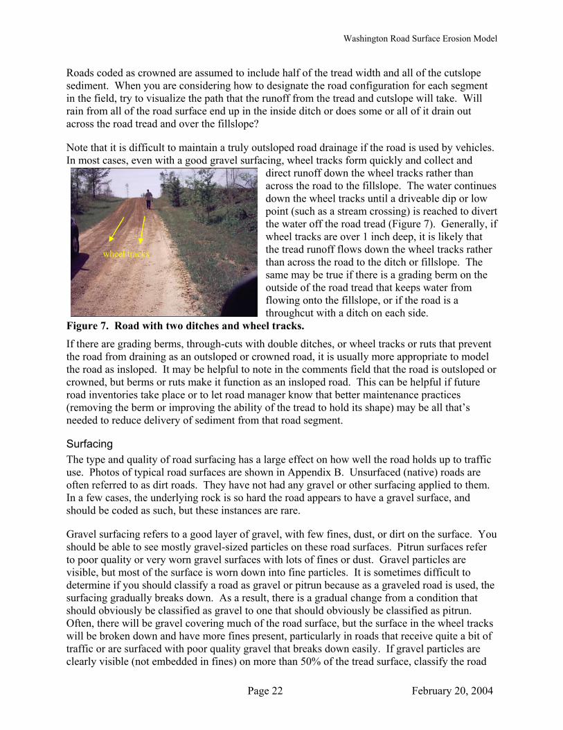
Note that it is difficult to maintain a truly outsloped road drainage if the road is used by vehicles. ing, wheel tracks form quickly and collect and direct runoff down the wheel tracks rather than across the road to the fillslope. The water continuesdown the wheel tracks until a driveable dip or low point (such as a stream crossing) is reached to divert the water off the road tread (Figure 7). Generally, ifwheel tracks are over 1 inch deep, it is likely that the tread runoff flows down the wheel tracks rather than across the road to the ditch or fillslope. Thsame may be true if there is a grading berm on the outside of the road tread that keeps water fromflowing onto the fillslope, or if the road is a throughcut with a ditch on each side.
Figure 7. Road with two ditches and
In most cases, even with a good gravel surfac
e
wheel tracks. ches, or wheel tracks or ruts that prevent
s
Surfacing d quality of road surfacing has a large effect on how well the road holds up to traffic
.
Gravel surfacing refers to a good layer of gravel, with few fines, dust, or dirt on the surface. You
, the
ks
wheel tracks
If there are grading berms, through-cuts with double ditthe road from draining as an outsloped or crowned road, it is usually more appropriate to model the road as insloped. It may be helpful to note in the comments field that the road is outsloped orcrowned, but berms or ruts make it function as an insloped road. This can be helpful if future road inventories take place or to let road manager know that better maintenance practices (removing the berm or improving the ability of the tread to hold its shape) may be all that’needed to reduce delivery of sediment from that road segment.
The type anuse. Photos of typical road surfaces are shown in Appendix B. Unsurfaced (native) roads are often referred to as dirt roads. They have not had any gravel or other surfacing applied to themIn a few cases, the underlying rock is so hard the road appears to have a gravel surface, and should be coded as such, but these instances are rare.
should be able to see mostly gravel-sized particles on these road surfaces. Pitrun surfaces refer to poor quality or very worn gravel surfaces with lots of fines or dust. Gravel particles are visible, but most of the surface is worn down into fine particles. It is sometimes difficult todetermine if you should classify a road as gravel or pitrun because as a graveled road is usedsurfacing gradually breaks down. As a result, there is a gradual change from a condition that should obviously be classified as gravel to one that should obviously be classified as pitrun. Often, there will be gravel covering much of the road surface, but the surface in the wheel tracwill be broken down and have more fines present, particularly in roads that receive quite a bit of traffic or are surfaced with poor quality gravel that breaks down easily. If gravel particles are clearly visible (not embedded in fines) on more than 50% of the tread surface, classify the road
Page 22 February 20, 2004
Washington Road Surface Erosion Model
as gravel. If the gravel particles are covered or embedded in fines on more than 50% of the roadsurface, classify the surfacing as pitrun.
If you are conducting road surveys during dry weather, the relative amount of dust kicked up by
hat
Ruts can greatly increase road surface erosion by collecting water and directing it down the ruts
Grass on a road surface can reduce erosion. Grass can either be planted or become established t
Average Tread Width road tread from the slope break at the fillslope side to the slope break at
passing vehicles can be a good indication of how worn the surface is. Large clouds of dust behind vehicles indicates that there are large quantities of fine particles on the road surface tcan be easily eroded. Little dust indicates that the road surface is in good condition, and there are not many fine particles available to erode. This method will only be helpful under dry conditions since recent rains or moist roads keep the dust down.
instead of off the road tread. Ruts are defined as wheel indentations over 2 inches deep. The model allows ruts to be applied to gravel- or native-surfaced roads.
naturally. Traffic or grading of the road surface will kill the grass and reduce its effectiveness areducing erosion. The model allows grass to be applied to native surfaced roads. If there is grass growing on other road surface types, these can be taken into account by the use of a Custom BMP (see Appendix C).
Measure the width of thethe ditch or cutslope side (see Figure 2). This width is generally the driveable width, and includes the full area of tread surfacing that could be driven on. It is wider than the width receives normal traffic. If there are wider areas in the road segment (pullouts or landings), thesareas should be taken into account when determining an average tread width.
that e
Traffic Use e may be best determined by talking with the land or road manager prior to or after
road
The traffic usgoing out in the field. It is difficult to determine accurately from field indications alone, although the general traffic patterns on the roads are usually evident based on wear on thetread. Traffic patterns also can vary considerably over time, so it is important to decide if you are attempting to model a long-term average traffic rate (over many years), or the effects of a single season’s use based on short-term timber harvesting and hauling activities. Table 6 describes typical traffic categories and the corresponding average number of passes per dalog trucks and pickups or cars.
y by
In order to determine which is the most appropriate traffic factor to assign to a segment, select
e.
by
ng-
the road use category that most closely fits the segment. Average traffic use for both log truck traffic and residential/recreational/administrative traffic (vehicles/day) is provided as a guidelinThe average vehicles/day values in Table 5 were based on traffic use averaged over all days in a year (including weekends and non-use periods). To determine the appropriate average use category, determine total trips/year on a road and divide by 365 days. Use of specific roadslog trucks changes over time as timber sales occur in different parts of a watershed. If the purpose of your modeling is to determine average road erosion in the watershed, pick the loterm average traffic rates on each road type. If the purpose of modeling is to determine sediment input from a specific timber sale, select use rates that best fit the traffic rates on that road during
Page 23 February 20, 2004

Washington Road Surface Erosion Model
the sale. If there are seasonal changes in traffic patterns that you would like to model (such as summer use only, or only winter haul on snow-covered roads) this can be accomplished by setting up a custom BMP. This procedure, described in Appendix C, allows the user to entespecific traffic level for each month of the year.
r a
Table 6. Traffic Use Categories.
Average p asses/dayog Pickup/
car
Heavy Highway Very heavy use by traffic throughout truck and carthe year. If surface is paved, see note below*. >5 >5
Heavily used by log truck traffic throughout the year; usually the main access road in a watershedthat is being actively logged.
Road Receives moderate use by logall or most of the year. Usually roads branching off main haul road that head up tributaries or thataccess large portions of the watershed.
Road Receives light log truck use during the yoccasionally be heavily used to access a timber sale. Receives car/pickup or recreational use. Short road used to access a single logging unit. Used to haul logs for a brief time while unit is logged. On the average receives little use.
(Inactive) blocked Road is blocked by a tank trap, boulders, etcno longer used by traffic.
Note: if road ffic levels a classified as “Heavy” and the su l
Traffic Category Road Class Description L
Truck
Mod. Heavy Main Haul
4-5 >10
Moderate
Primary trucks throughout
3-4 5-10
Mod. Light Secondary ear. May
1-2 1-5
Light Spur Road
<1 <1
Abandoned Abandoned/ . or is 0 0 * tra re rface is asphalt, check to make sure the mode
Cutslope Cover Density , slash, and other materials can protect bare soil on a cutslope from
s
e,
Cutslope Average Height slope is measured as the slope length from the top of the cut to the
results are reasonable. There will be little erosion from the paved surface, but the increased runoff could result inmore ditch erosion.
Vegetation, rocks, leaf littererosion. The percentage of soil that is protected, or covered by any of these items, is recorded athe cutslope cover density. Since it is difficult to estimate cover precisely, six different cover ranges are used. Another way to estimate this value is to determine how much bare soil you seand subtract that percentage from 100%. For example, if you see bare soil over 20% of the area, the cover value is 80% (100%-20%).
The average height of the cutbottom of the slope (the location where the cutslope intersects either the top of the ditch or the road tread; see Figure 2). This value is often quite variable along a road segment. At a stream crossing segment, cutslope height can vary from no cutslope at the crossing to over 25 feet highalong upslope portions of the road that are cut into the hillside. Take into consideration the amount of cutslope of different heights in your evaluation. Record an average height by
Page 24 February 20, 2004
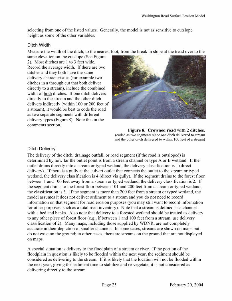
Washington Road Surface Erosion Model
selecting from one of the listed values. Generally, the model is not as sensitive to cutslope height as some of the other variables.
Ditch Width Measure the width of the ditch, to the nearest foot, from the break in slope at the tread over to the same elevation on the cutslope (See Figure 2). Most ditches are 1 to 3 feet wide. Record the average width. If there are two ditches and they both have the same delivery characteristics (for example two ditches in a through cut that both deliver directly to a stream), include the combined width of both ditches. If one ditch delivers directly to the stream and the other ditch delivers indirectly (within 100 or 200 feet oa stream), it would be best to code the roaas two separate segments with differdelivery types (Figure 8). Note this in thecomments section.
f d
ent
Figure 8. Crowned road with 2 ditches. (coded as two segments since one ditch delivered to stream and the other ditch delivered to within 100 feet of a stream)
Ditch Delivery The delivery of the ditch, drainage outfall, or road segment (if the road is outsloped) is determined by how far the outlet point is from a stream channel or type A or B wetland. If the outlet drains directly into a stream or typed wetland, the delivery classification is 1 (direct delivery). If there is a gully at the culvert outlet that connects the outlet to the stream or typed wetland, the delivery classification is 4 (direct via gully). If the segment drains to the forest floor between 1 and 100 feet away from a stream or typed wetland, the delivery classification is 2. If the segment drains to the forest floor between 101 and 200 feet from a stream or typed wetland, the classification is 3. If the segment is more than 200 feet from a stream or typed wetland, the model assumes it does not deliver sediment to a stream and you do not need to record information on that segment for road erosion purposes (you may still want to record information for other purposes, such as a total road inventory). Note that a stream is defined as a channel with a bed and banks. Also note that delivery to a forested wetland should be treated as delivery to any other piece of forest floor (e.g., if between 1 and 100 feet from a stream, use delivery classification of 2). Many maps, including those supplied by WDNR, are not completely accurate in their depiction of smaller channels. In some cases, streams are shown on maps but do not exist on the ground; in other cases, there are streams on the ground that are not displayed on maps.
A special situation is delivery to the floodplain of a stream or river. If the portion of the floodplain in question is likely to be flooded within the next year, the sediment should be considered as delivering to the stream. If it is likely that the location will not be flooded within the next year, giving the sediment time to stabilize and re-vegetate, it is not considered as delivering directly to the stream.
Page 25 February 20, 2004
Washington Road Surface Erosion Model
Ditch Condition The condition of the ditch can have an influence on whether the ditch traps sediment, erodes and produces additional sediment, or merely conveys sediment that flows into it from the cutslope and tread. The model does not use ditch condition in erosion calculations at this time, but future updates may include this capability. Record the conditions of the ditch: stable (no evidence of downcutting); rocked/vegetated; or eroding (evidence of downcutting or gullying in the ditch).
BMPs The application of some Best Management Practices (BMPs) can change the erosion or delivery potential of a road segment. The model allows the user to specify BMPs for each road segment, if desired. This option lets users track actual BMPs that have been applied to the road by choosing from either a “standard” list of BMPs or a custom BMP the user creates.
If BMPs have been applied to road segments, they should be noted by number and date applied (if known) during the field inventory. A list of standard BMPs is included on a 1-page sheet in Appendix B. A complete description of standard BMPs and how the model accounts for them is included in Appendix C. If you will be recording data on BMPs for your road inventory area, refer to Appendix C for more information.
Problem Area/Comments Road segments may have special situations or problems that are not included in the surface erosion model, but are of interest to the landowner. A list of common road problems is included in Appendix B. The comment field allows you to note these items, or to include other remarks.
Class The road class is an optional field. It is not used in model calculations, but may be useful to the landowner for later classifying or sorting the road database. Road classes can be chosen from those listed in Table 5.
Position Road position is an optional field. It is not used in model calculations, but may be useful to the landowner for later classifying or sorting the road database. This field refers to the position of the road segment in the landscape. Possible entries are ridgetop (on top of the hill – likely does not deliver to streams); midslope (on the side of a hill); stream adjacent (parallel and close to a stream or waterway); and flat valley bottom (within a broad, flat stream valley, but not adjacent to the stream or waterway).
Base Map Note that each segment should have a unique segment number. Record that segment number on your field map as well as the data form, so that you can find the segments in the future. It is often helpful to record the approximate start and end point of each segment on the map. Coloring or highlighting delivering segments may also be helpful for future reference. A sample field map and corresponding data sheet are shown in Figure 9.
Page 26 February 20, 2004
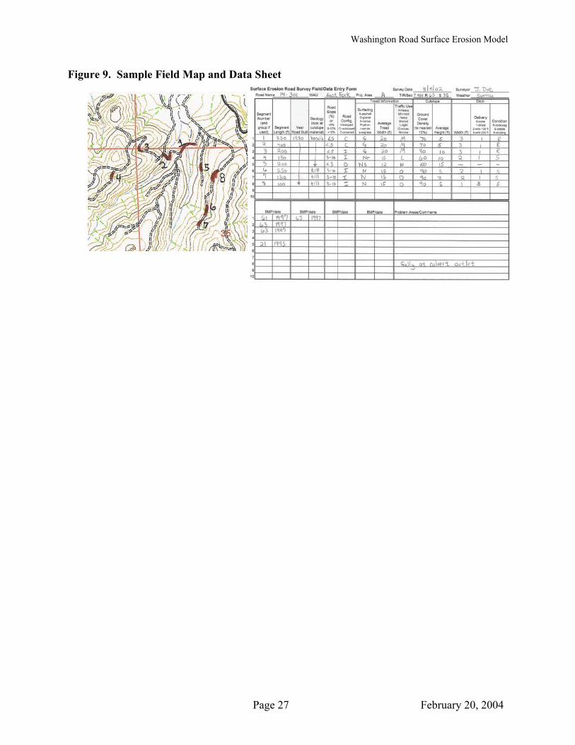
Washington Road Surface Erosion Model
Figure 9. Sample Field Map and Data Sheet
Page 27 February 20, 2004

Washington Road Surface Erosion Model
Chapter 5 Access Application
The Washington Road Surface Erosion Model (WARSEM) calculations are programmed into a database application. This application has been coded into an Access module that can be loaded and used on any PC with Windows 98 or higher. The application requires 140 MB of disk space. The user does not need to have a copy of the Microsoft Access program installed on their computer. The following sections provide instructions on how to load the application onto your computer, import or enter data, and perform model runs.
5.1 Loading the Application
WARSEM is distributed in three formats. Users with Access installed on a personal computer can install a version of the application that will allow the user to take advantage of all the functions of Access. Microsoft Access 97 and Microsoft Access 2000 use different internal file formats for the database file. For this reason there are two setup files available for users with Microsoft Access installed on their PCs:
• Setup97.exe will install the Access 97 database application.
• Setup2K.exe will install the Access 2000 database application (use for XP).
Users who do not have Access installed on their computer can install the runtime version of the application that will allow complete access to the model functions but without the benefit of additional utilities that only comes with a purchased copy of Access. Users without Microsoft Access installed on their computer will need to use the SetupRT.exe installation file.
Setup files can be obtained from the Washington Department of Natural Resources. The setup file will initiate an installation process that creates folders, copies files, and creates an application short cut on the user’s Start Programs menu.
To install the application, close all programs and run the appropriate setup file (Setup97.exe, Setup2K.exe, or SetupRT.exe) by double clicking on the file from Windows Explorer. The first screen will appear as:
Page 28 February 20, 2004

Washington Road Surface Erosion Model
Click on “Next” and follow the instructions on the following screens. The install program will copy all necessary program files to a new WARSEM subdirectory in the Program Files directory on your C drive. Sample data files will also be copied into a Projects subdirectory under the WARSEM directory. After you complete the installation, you should restart your computer. The final screen will appear, indicating you have successfully installed the program:
5.2 Starting the Application
Once installed, the Washington Road Surface Erosion Model can be launched from the list of programs in the Windows Start Programs WARSEM menu. Clicking on this shortcut will launch the startup window:
There are 3 different ways to start working on data in the WARSEM application:
• Use a Wizard – the program will guide you through entering all the required start-up data for a new project file.
Page 29 February 20, 2004

Washington Road Surface Erosion Model
• Start from Scratch – for experienced users who do not want to use the Wizard to enter start-up data.
• Open a Project – to open an existing project file.
Use a Wizard This button will launch a form that will provide the following input screen:
This first page of the wizard directs you to enter a file name for the Access database application. You are also required to select the primary WAU for the project area from a drop-down menu. If you are unsure of the correct WAU for your project area, contact your regional WDNR office for assistance. The menu includes WAU and WRIA name since there are duplicate WAU names in the state. If the project area spans more than one WAU, you will be able to set up another project area within the Access application once it starts and you have added data. You also input the number of miles of stream within the project area. This will allow you to compute FFR metrics (the number of stream miles can be obtained from WDNR – contact your regional office).
You must also select a choice from the Data Resolution buttons. WARSEM records data resolution in terms of the scale of maps used to collect data. The highest resolution would include direct measurements recorded in the field. Medium resolution would include measurements recorded from a source such as ortho rectified photography or GIS data captured at a scale near 1:12,000. Lower resolution would include the use of data at scale of 1:24,000 or smaller. Smaller scale indicates more land coverage is depicted for a given area on a map. The smaller the scale, the more difficult it is to discern and measure features accurately.
When you have filled in all required fields, click the “Next” button. You can click the “Back” button at any time if you need to correct data on a previous screen. Clicking the “Close” button will return you to the startup form.
Page 30 February 20, 2004

Washington Road Surface Erosion Model
The second page of the New Project Wizard asks you how you intend to use the data. This relates to the Applications Matrix (Table 1) and will be used in the Access application to determine required fields and for project summary reports. Click on the appropriate Level for your application, then click “Next.”
Page 3 of the New Project Wizard asks you to identify the source for the data you wish to use. If you will be importing data from a SEDMODL run or from an existing dBASE file or Excel spreadsheet, you will be prompted with a dialog box to indicate the location of the input file (see Section 5.3 for a description of importing data). If you want to enter road information within the application, click on the “Input road data using a form” button. Click on the “Finish” button when you are ready to proceed to data entry/editing and calculating delivered sediment (see Section 5.4).
Page 31 February 20, 2004

Washington Road Surface Erosion Model
Start From Scratch If a user wants to start a new project in Start From Scratch mode, a switchboard style menu is presented to the user after the new project file is opened to help guide them through the data required to build a project file.
The order of the menu choices represents the recommended order of activities when setting up a project from scratch. The first step is to develop one or more Project Area descriptions using the Project Area Builder
Six items define a project area, five of which are required to be provided.
1. Project area is a user-defined number that when grouped with a WAU name creates a unique combination. Project Areas must be contained within a single WAU.
2. Management Blocks are used when creating Road Management and Abandonment Plans (RMAP) and can be used to describe an area that may include roads within one or more WAUs. In WARSEM, Management Blocks provide one way to group roads for
Page 32 February 20, 2004

Washington Road Surface Erosion Model
modeling and reporting. Management Blocks can occur across multiple Project Areas and WAUs.
3. Each WAU has an associated number of miles of streams that have been determined by the WDNR and are used to calculate FFR monitoring metrics. You can contact a WDNR Regional Office if you don’t have this information.
4. An Application Level must be assigned to the data based on the quality of the road data. (See Table 1)
5. The quality of the map or GIS data must be assigned to the project using the description listed above in Data Quality.
Once the user clicks on the “Add” button, the data entry controls are enabled and the required fields highlighted in blue. Once the required data is entered the user can click on the save button to record the information about the new Project Area. After the data is saved it will become visible in the Existing Project Areas data frame portion of the form and available for editing. More than one Project area can be added.
The next steps in the Start From Scratch mode are to set the road data entry defaults and to enter or import road data. The “View Road Data Entry/Edit Defaults” screen is described in Section 5.4. The “Import Road Data into Project” screen is described in Section 5.3.
Open an Existing Project If you already have entered a data file and would like to continue to work on that file, choose the “Open a Project” button, and a list of recently used files will appear in the window:
Click on the “More files” and a screen will appear that allows you to chose from all files in the Projects subdirectory of the WARSEM directory, or to navigate to another file location on your computer. Select the appropriate file to open. The file will be loaded into the application, and the data entry/edit screen will appear. Go to Section 5.4 for information on how to proceed to edit or enter data.
Page 33 February 20, 2004

Washington Road Surface Erosion Model
5.3 Importing Data
WARSEM allows you to import existing road data from other applications if the data is saved in one of three formats, and is formatted correctly for importing. The three acceptable input methods are:
• Importing data from a SEDMODL2 model run • Import data from a dBase or Excel file • Import from a comma delimited text file.
VERY IMPORTANT: You must prepare the import file in advance so that the data are in the correct order and have the correct information in each field. Data imported from any dBase, Excel, text, or SEDMODL2 file must be prepared (see Appendix E for these requirements).
SEDMODL2 is a GIS application that computes road surface erosion. Even though SEDMODL2 is only supported for ArcInfo, other GIS applications can be used to identify and attribute road features with information that can be utilized by WARSEM, assuming the GIS application has the ability to export the data to a dBase format or comma delimited text file, or a format that can be imported into another application that can produce a dBase file or comma delimited text. Excel can import several different data formats and export a dBase or comma delimited file.
The data identified for import from a dBase or Excel file or from a comma delimited text file must be specifically formatted so that the WARSEM application can recognize and import the data into the appropriate fields. Please refer to Appendix E for information on data format requirements for import into WARSEM.
If you have selected to import data from another application, a Data Import Dialog Screen will appear:
Click on the “Next” button. The second page allows you to select the source of the data you wish to import, if the first row of your file has header information, and if you would like to replace or append (add to existing records) the imported data to any records if you already have a file opened.
Page 34 February 20, 2004
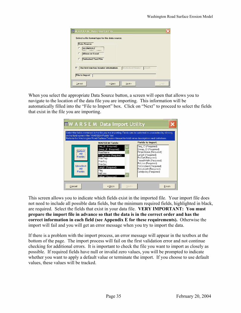
Washington Road Surface Erosion Model
When you select the appropriate Data Source button, a screen will open that allows you to navigate to the location of the data file you are importing. This information will be automatically filled into the “File to Import” box. Click on “Next” to proceed to select the fields that exist in the file you are importing.
This screen allows you to indicate which fields exist in the imported file. Your import file does not need to include all possible data fields, but the minimum required fields, highlighted in black, are required. Select the fields that exist in your data file. VERY IMPORTANT: You must prepare the import file in advance so that the data is in the correct order and has the correct information in each field (see Appendix E for these requirements). Otherwise the import will fail and you will get an error message when you try to import the data.
If there is a problem with the import process, an error message will appear in the textbox at the bottom of the page. The import process will fail on the first validation error and not continue checking for additional errors. It is important to check the file you want to import as closely as possible. If required fields have null or invalid zero values, you will be prompted to indicate whether you want to apply a default value or terminate the import. If you choose to use default values, these values will be tracked.
Page 35 February 20, 2004

Washington Road Surface Erosion Model
5.4 Inputting and Editing Road Data
When you begin a new project session and are ready to input or edit road data using a form, a log on screen will appear that allows you to enter your name if desired. Entering your name will allow the application to track who is editing data records.
If you do not want to enter your name, you can select “Cancel” and/or select “No thanks, don’t ask me again.”
Selecting Default Values The WARSEM application allows users to select default values to fill into new data records. This makes it easier if you have lots of data to enter that have similar values (for example, if most of your roads are native surfaced with light traffic factors, you can instruct the application to enter those values in all new records to save you the time of selecting those values in each record). You can select which attributes you want the application to remember as well as the default value for each of those attributes. When working on a specific data record, you can always override any of the default values. You can also change the default values at any time during the data entry/edit session. For example, if most of your roads are native surfaced, but you have 20 road segments that are gravel surfaced, you can go to the appropriate default values screen and change the default surfacing value to “Gravel”, enter the 20 road segments, and then change the default value back to “Native.”
Depending upon which start-up method you chose, you will either be taken to the Road Attribute default entry form, or you can navigate to it at any time using the menu bar by selecting Options
Menu/Forms Show Update Tracking Options. The first screen will appear, which allows you to select those attributes you’d like the application to remember and use to fill in new data records.
Page 36 February 20, 2004

Washington Road Surface Erosion Model
Select those fields that you would like the application to remember. Then select the “Road Condition Defaults” tab to display the next screen. Select the appropriate road condition default values.
Page 37 February 20, 2004

Washington Road Surface Erosion Model
If you wish to enter default Road Class values, select the “Road Class” tab and select the appropriate values. When you are finished, select the “OK” button.
Entering and Editing Data Depending on the startup method chosen, you will either be automatically taken to the data input form, or you will have an empty project screen. If you have an empty screen, select the data import form from the drop-down menu list at the top of the screen. Select Options Menu/Forms Browse – Edit Road Data.
Page 38 February 20, 2004

Washington Road Surface Erosion Model
If you would like to enter or edit road segments within the Access Application, the following data entry form will appear. This data entry form closely follows the road field form.
Verify and save new record
Add BMP
The form is divided into topic areas that relate to the field form. Required fields are highlighted (based on the model Level chosen initially) to remind you to provide this basic data. Some fields allow entry only from a dropdown list rather than direct entry. Selecting a Project Area automatically fills in the WAU name associated with that project. Entry of Township Range and Section numbers are used to assign Geologic Erosion Rate and Rainfall Factors.
To simplify data entry for large numbers of records, you can instruct the model to remember specific field values and apply these automatically to new records as described in the previous section.
After you have finished entering data for a record, click on the Validate and Save New Record button. You can also enter BMPs for the record using the Add BMP button. For instructions on entering Best Management Practices (BMPs), see Section 5.5.
After you have entered data records, additional buttons will appear on button line that allow you to navigate through the existing records in the database. If you pause your mouse arrow over each of the buttons, it will tell you the function of that button.
Page 39 February 20, 2004

Washington Road Surface Erosion Model
At the end of the data entry section, you can select “Exit” from the File menu to close the program or continue on to run the model calculations as described in Section 5.7.
Editing Existing Data The data entry form can be used to edit data imported from external sources or to edit data you have entered previously using the form. You can change road attributes or apply BMPs. Application of BMPs is described in Section 5.5.
When you edit data in a pre-existing data record, the application will ask you the purpose of the edit. This is done to enable tracking of changes to the road network through time. If you are planning to use the ability of the application to track changes, fill in the appropriate information in the window. You can select the purpose of the edit for each record you are editing, or you can tell the program that all edits will be for the same purpose. You can also select the option to not track changes to prevent the application from asking you about every change you make if you don’t want to track changes.
5.5 Applying BMPs and Creating Custom BMPs
You can use the WARSEM application to track BMPs that you apply to improve road conditions. A list of Standard BMPs is described in Appendix C. You can also create Custom BMPs if you use BMPs not included on the standard list as described in Appendix C, Section C.7.
There are two methods to add BMPs to road segments: (1) clicking on the “BMP” button on the Data Entry/Edit Screen (button is the last in the row of buttons at the top of the screen); or (2) using the BMP manager screen to apply one or more BMPs to a road segment.
Page 40 February 20, 2004
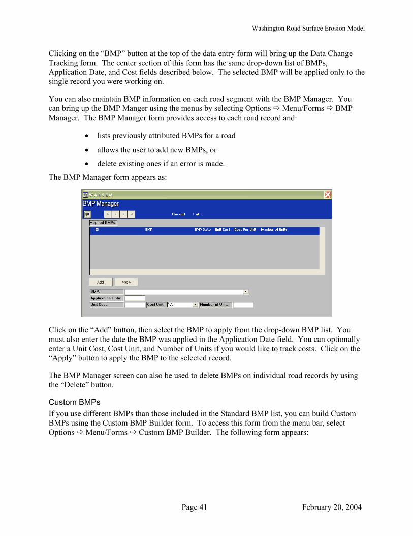
Washington Road Surface Erosion Model
Clicking on the “BMP” button at the top of the data entry form will bring up the Data Change Tracking form. The center section of this form has the same drop-down list of BMPs, Application Date, and Cost fields described below. The selected BMP will be applied only to the single record you were working on.
You can also maintain BMP information on each road segment with the BMP Manager. You can bring up the BMP Manger using the menus by selecting Options Menu/Forms BMP Manager. The BMP Manager form provides access to each road record and:
• lists previously attributed BMPs for a road
• allows the user to add new BMPs, or
• delete existing ones if an error is made.
The BMP Manager form appears as:
Click on the “Add” button, then select the BMP to apply from the drop-down BMP list. You must also enter the date the BMP was applied in the Application Date field. You can optionally enter a Unit Cost, Cost Unit, and Number of Units if you would like to track costs. Click on the “Apply” button to apply the BMP to the selected record.
The BMP Manager screen can also be used to delete BMPs on individual road records by using the “Delete” button.
Custom BMPs If you use different BMPs than those included in the Standard BMP list, you can build Custom BMPs using the Custom BMP Builder form. To access this form from the menu bar, select Options Menu/Forms Custom BMP Builder. The following form appears:
Page 41 February 20, 2004
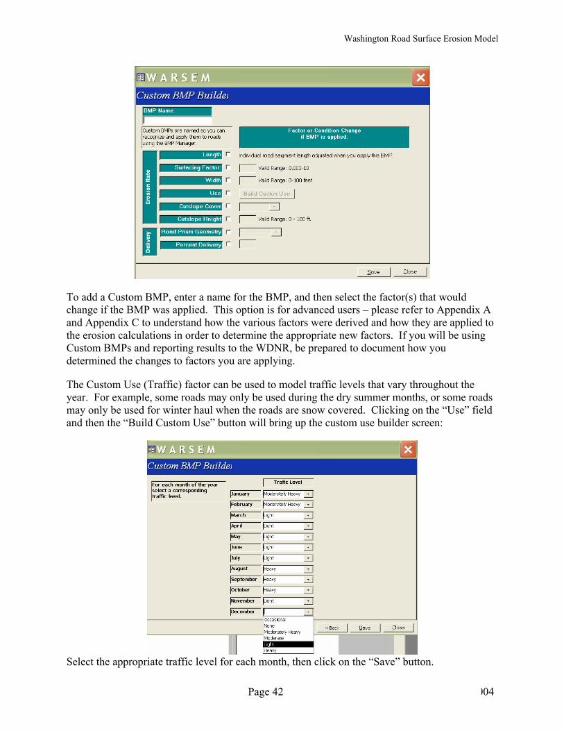
Washington Road Surface Erosion Model
To add a Custom BMP, enter a name for the BMP, and then select the factor(s) that would change if the BMP was applied. This option is for advanced users – please refer to Appendix A and Appendix C to understand how the various factors were derived and how they are applied to the erosion calculations in order to determine the appropriate new factors. If you will be using Custom BMPs and reporting results to the WDNR, be prepared to document how you determined the changes to factors you are applying.
The Custom Use (Traffic) factor can be used to model traffic levels that vary throughout the year. For example, some roads may only be used during the dry summer months, or some roads may only be used for winter haul when the roads are snow covered. Clicking on the “Use” field and then the “Build Custom Use” button will bring up the custom use builder screen:
Select the appropriate traffic level for each month, then click on the “Save” button.
February 20, 2004 Page 42

Washington Road Surface Erosion Model
5.6 Using Model Menus
There are six possible menu selections in the menu bar of the WARSEM application. These are displayed near the top of the application screen. For users running either the Access2K or Access97 versions of the application, the default Access menus are hidden to avoid confusion with application menus. If you would like to use the normal Access menus, press the F11 key to display default menus. All normal Access functions can be used to work with the WARSEM database.
File The File menu is similar to the file menus in most programs: the user can choose to Close the current file, Search for a new file, or Exit the program.
Selection The Selection menu item allows the user to select records from the database that match a specified set of criteria. This allows the user to select, for example, all gravel surfaced roads, or all insloped roads, or all roads with over 5 tons of sediment/year. A user can also select roads segments with a combination of criteria, such as all native surfaced roads over 10% gradient. The user selects records using menu choices that increment a special field in each record called “Flag.”
Each database record contains a field labeled “Flag.” The Flag field is incremented by 1 each time the record is selected using the selection process. The user can increase or decrease the Flag field in one or all records using the “Add by….” menu items or the flag menu items at the bottom of the menu.
The Selection menu appears as follows:
Page 43 February 20, 2004

Washington Road Surface Erosion Model
The effect of the menu choices on the Flag field is described in Table 7.
Table 7. Use of Selection Menu Choices.
Menu Choice Effect on “Flag” field View Selection Shows options for viewing flagged records (four different tables may be
viewed). Select No Records Changes the Flag value to 0 in all records. Select All Records Changes the Flag value to 1 in all records. Select Active Table Selects either the Master Road Table or a saved copy of the road table to
use to perform model functions. Show Active Table Displays a dialog box indicating the name of the current Active Table. Add by ……. Adds 1 to the Flag field in records that meet the specified criteria. Promote Selection Adds 1 to the Flag field in all records. Demote Selection Subtracts 1 from the Flag field in all records. Toggle Flag Switches the values of the Flag and Old Flag fields. Set Flag>0 to 1 Sets all records with a Flag value of greater than 1 to a Flag value of 1. Save Flag to Old Flag
Saves values in the “Flag” field to the “Old Flag” field to allow user to try a different set of selection procedures while saving the current Flag field
Restore Flag from Old Flag
Moves the value in the “Old Flag” field back into the current “Flag” field.
The first step in using the “Selection” menu items is to Select the Active Table (either the Master Road Record table or a named scenario the user has saved). If no table has been selected, an error message will appear.
The following example shows how to use this function to select specific records using the “Add to….” menu choices. Suppose you want to isolate records where:
• the surface type is Pit Run • the level of use is Moderate and, • total sediment production is greater than or equal to 10.
This can be done in three steps:
Step 1. 1. First select “Select No Records” to set Flag = 0, then select “Add by Surface Type” by selecting Selection Add by Surface Type from the menu.
Select “Add by Surface Type”
2. You will then be presented with the following dialog box.
Page 44 February 20, 2004

Washington Road Surface Erosion Model
Select “Pit Run” from the dropdown list.
3. The following message box is presented.
A message box indicates the success of the query and the number of the records added.
Step 2.
1. Select “Add by Use Type” from the “Selection” menu. You will be presented with the following dialog:
Select “Moderate” from the dropdown list.
2. The query yields the following result.
3. To select ONLY the road segments that meet both requirements (road surface = pitrun and use type = moderate), select “Demote Selection” from the menu. This subtracts 1 from all flag values, resulting in a flag value of 1 for records meeting both requirements, a value of 0 for records meeting only 1 requirement, and a value of -1 for records meeting neither requirement.
Page 45 February 20, 2004

Washington Road Surface Erosion Model
Step 3.
1. After selecting “Add By Total Sediment” from the menu you will be presented with the following dialog box:
Click on Ok to complete the query.
Type in the value you wish to use to select records.
Select the operand you want to compare the numeric values to.
2. A message box will confirm the results of the query.
3. To select ONLY the road segments that meet all requirements, select “Demote Selection” from the menu.
At this point records that have met all three requirements will have a flag value of 1. You can proceed to view these records using the “View Selection” menu choice, or you can update selected records as described in the next section.
The “View Selection” menu has several choices to allow the user to directly view the selected road segment records.
The “Master Roads Table Flag Tally” shows the total number of records and sediment production from flagged records:
The “View Active Flag Table” allows the user to view road sediment summary information based on the current value of Flag. Each “Add To Flag” action increments the value of Flag by
Page 46 February 20, 2004

Washington Road Surface Erosion Model
one. If the user keeps notes about how the queries are done, they will know what the Flag value means. For example, if you “Add to Flag” for surfacing where roads are pit run and then “Add to Flag” for road gradient where gradient is greater than 10%, the records that satisfy the first query will have a Flag value of 1 and the records that satisfy both queries will have a Flag value of 2.
The “View WARSEM Table” menu item shows the raw data file that contains road records. Use the slider button at the bottom of this screen to move back and forth through the data fields in a record.
VERY IMPORTANT: It is possible to change the values of road segment fields in the View WARSEM Table view. However, the model will not track the changes or reason for changes to the records if used in this manner. MAKE SURE YOU ONLY MAKE EDITS USING THE DATA ENTRY/EDIT SCREEN IF YOU WANT TO TRACK CHANGES.
Updates Flagged records can be edited to change values of different fields. This can be used, for example, to determine the effects of adding gravel to native surfaced roads, changing insloped roads to outsloped roads, changing traffic values, etc. The Update menu choice shows the following screen:
Page 47 February 20, 2004

Washington Road Surface Erosion Model
The user can select the desired field they would like to change. Selecting a field brings up the Scenario Preference screen, which asks the user if they would like to make a copy of the master road data before applying the selected updates.
VERY IMPORTANT: Make sure to make a copy of the master road data before you apply any updates if you are running scenarios and would like to return back to the original values when you are done. IF YOU DON’T MAKE A COPY OF THE MASTER ROAD DATA, YOU WILL LOOSE THE ORIGINAL DATA VALUES.
Make the appropriate selection from the Scenario Preference screen and hit “OK”. This will bring up an Update Screen that allows the user to change all records with Flag greater than 0 to a different value.
Page 48 February 20, 2004
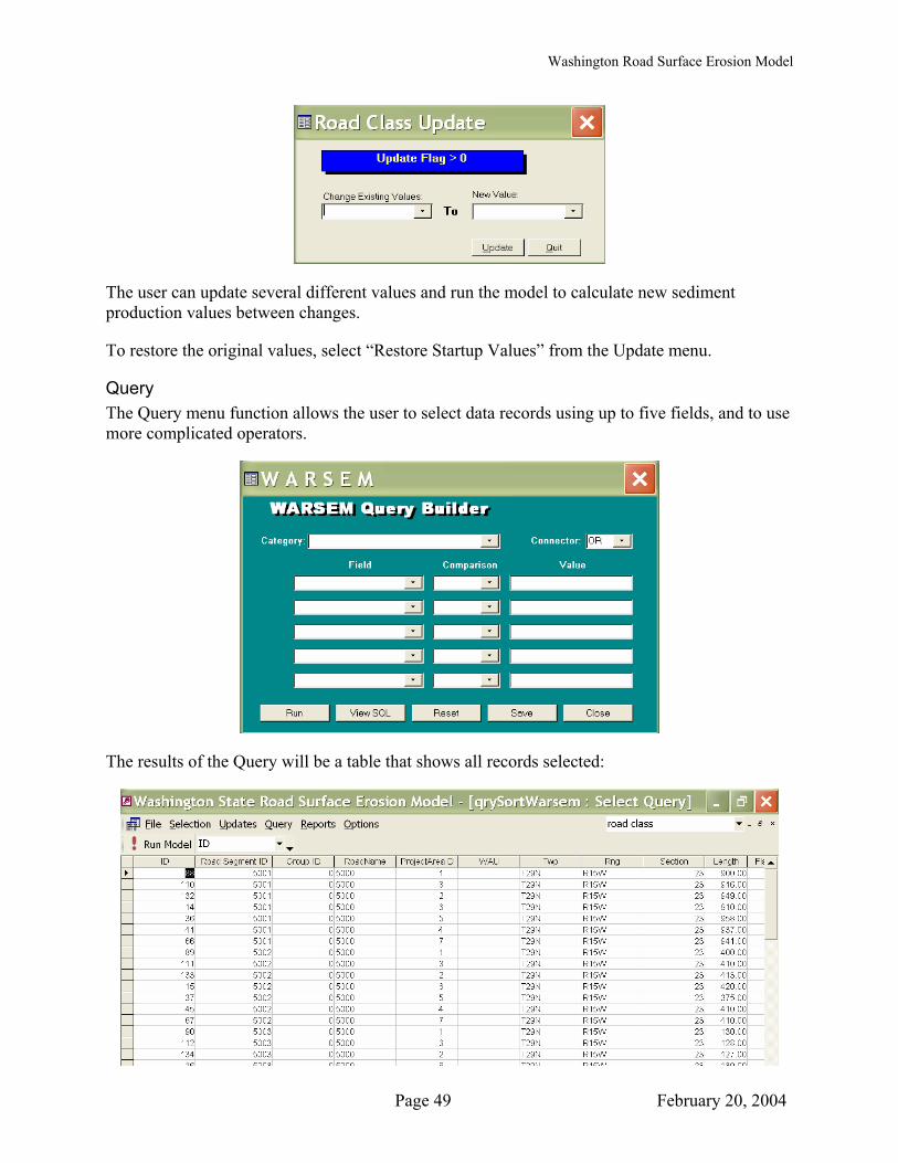
Washington Road Surface Erosion Model
The user can update several different values and run the model to calculate new sediment production values between changes.
To restore the original values, select “Restore Startup Values” from the Update menu.
Query The Query menu function allows the user to select data records using up to five fields, and to use more complicated operators.
The results of the Query will be a table that shows all records selected:
Page 49 February 20, 2004
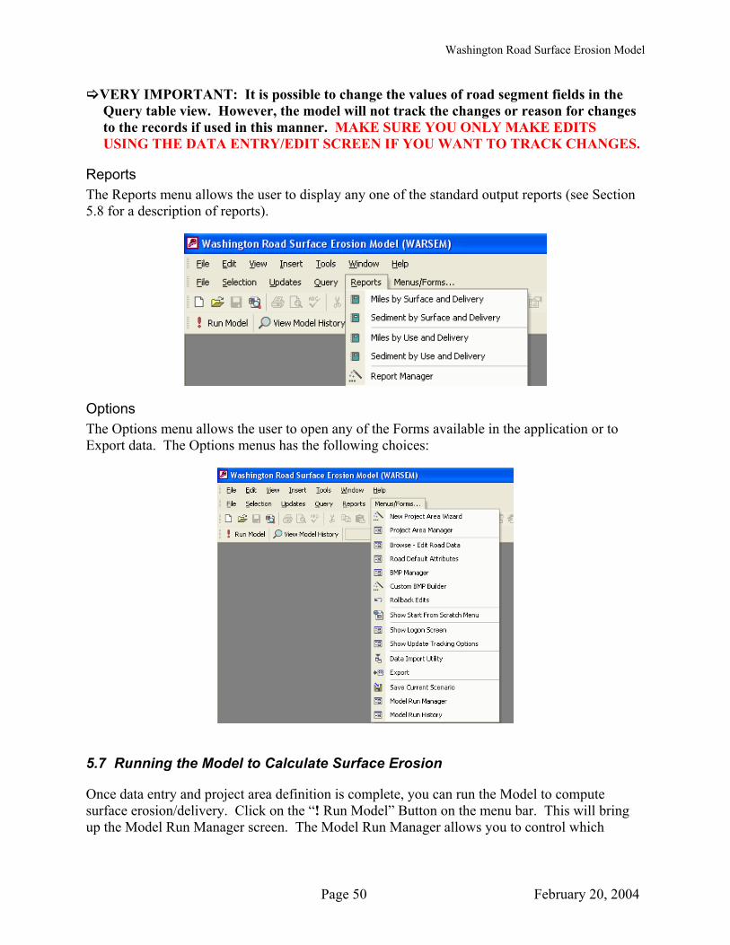
Washington Road Surface Erosion Model
VERY IMPORTANT: It is possible to change the values of road segment fields in the Query table view. However, the model will not track the changes or reason for changes to the records if used in this manner. MAKE SURE YOU ONLY MAKE EDITS USING THE DATA ENTRY/EDIT SCREEN IF YOU WANT TO TRACK CHANGES.
Reports The Reports menu allows the user to display any one of the standard output reports (see Section 5.8 for a description of reports).
Options The Options menu allows the user to open any of the Forms available in the application or to Export data. The Options menus has the following choices:
5.7 Running the Model to Calculate Surface Erosion
Once data entry and project area definition is complete, you can run the Model to compute surface erosion/delivery. Click on the “! Run Model” Button on the menu bar. This will bring up the Model Run Manager screen. The Model Run Manager allows you to control which
Page 50 February 20, 2004

Washington Road Surface Erosion Model
records are modeled, either by selecting records with a specific “flag” value, or by selecting a specific year to model. This dialog appears as:
The first item to fill out on the Model Run Manager screen is the Active Table. Click on the “Select Action Table” button and select the table you wish to use for the model run. The Master Roads Table is the original table of road values. If you are running different scenarios, several tables may be listed with the different scenarios you have made. You can run the model at various scales by using the Flag attribute to select a single road segment or a larger area such as a project area. Additionally, you can run the model using road conditions in place during a specific time period.
By indicating a specific Model Run Year, the model will ignore all roads with a construction date more recent than the specified model year. Roads that would have been new (<2 years) at that point in time will be modeled as new roads. BMPs applied prior to the Model Run Year will be used. This is useful to determine sediment production at one specific point in time. Note that you must have entered a construction year for the road data to run by model year.
You can also run the model in time steps for a specified range of dates. The Start Date and End Date values determine the range of time that the model will roll back to and the Step Value determines the yearly increment that the specified time period will be divided into. Prior to initiating a model run, the application will validate the range of dates that BMPs have been applied and notify you so that you can halt the process and specify a different time range. If a Start Date is older than the earliest BMP application date, the application will model roads for each step year by evaluating the age of the road and adjust sediment production based on road age; the same holds true for roads newer than the most recent BMP application date. Note that you must have entered a construction year for the road data to run by BMP application date.
Page 51 February 20, 2004

Washington Road Surface Erosion Model
5.8 Output Reports
The model will produce output reports that detail the information used to produce the results, aswell as numerical results indicating average annual sediment delivered to streams in the modarea. Reports can be accessed by selecting Reports from the menu and then selecting the appropriate report:
eled
The format and information included in the report will vary slightly based on the Model Level run. The first four reports listed provide basic summary data about all the records in the database. A sample Sediment by Use and Delivery output report is shown below.
The Report Manager selection allows you to select from a variety of report formats, and sinformation on all the records in the database or only flagged records. You will ne
elect ed to select
the type of report from the Report Type drop down menu as well as the road record table you want to use for the report (usually the Master Roads Table unless you have saved alternate scenarios).
Page 52 February 20, 2004

Washington Road Surface Erosion Model
The four types of reports in the Report Manager are:
WARSEM Summary Report – Summarizes sediment output for specified records.
WARSEM FFR Metrics – Provides information that enables user to calculate the Fish and Forest Rules monitoring metrics for the chosen roads (total miles of roads delivering, total sediment delivered, total miles of streams in the project area).
Best Management Practices – Provides information on BMPS that were applied to each record.
Model Detail Report – Lists input data and sediment production for each record.
ote that the Best Management Practices and Model Detail reports are formatted to be printed on
t. ager
port window showing model output will remain on the screen. You can maximize the window and/or zoom in by clicking within the report window to enlarge the results. You can also print out reports using the “File enu bar in Access.
5.9 Exporting records
WARSEM databases can be exported for use in ot the Options menu to bring up the Export Utility screen.
Nlegal size paper because of the amount of data for each record.
After selecting the report type and report table, click on the “Preview” button to view the reporIf you want to move into the report window, click on the “Cancel” button in the Report Manwindow. The re
Print” selection from the upper m
her programs. Select the “Export” option from
Page 53 February 20, 2004

Washington Road Surface Erosion Model
Data can be exported as a Dbase, Excel, or text file. All records in the database or only flagged records can be exported. Clicking on the “Export” button will prompt you to enter the file name for the export file.
er
talled. These files can be moved to another location and documented through the application control panel by selecting “More Files…” selection under Open an Existing
dates the location of the file. In a networked environment, a Project File could be kept on a server that is accessible to several people. Installing the application on
t designed for a multi-user environment and record locking may create accessibility problems.
5.10 File management
All projects created through the WARSEM control panel are kept in the Projects folder undWARSEM directory located in the Windows Program Files directory on the drive where the program was ins
Project. The application up
client machines and directing the application to the location of the shared file will allow multiple users to access the data. However, this application was no
Page 54 February 20, 2004

Washington Road Surface Erosion Model
Chapter 6 Interpreting Model Results
The Washington Road Surface Erosion Model estimates the average annual amount of road surface erosion delivered to streams from each road segment. The computed amount of sediment should be regarded as a long-term estimate of sediment that would be produced from a road with similar characteristics under climatic conditions similar to those at the road location. The actual amount of sediment from any given road segment may be different that the predicted amount due to inter-annual variations in weather and traffic patterns and local changes in topography and soil characteristics that cannot be accounted for in the model. It is important to keep these limitations of the model results in mind when attempting to interpret the numerical results. It is appropriate to look at the relative differences in erosion estimates when comparing watershed areas or road segments, but the sediment values in tons/year should always be regarded as estimates not absolute values.
Page 55 February 20, 2004

Washington Road Surface Erosion Model
Page 56 February 20, 2004
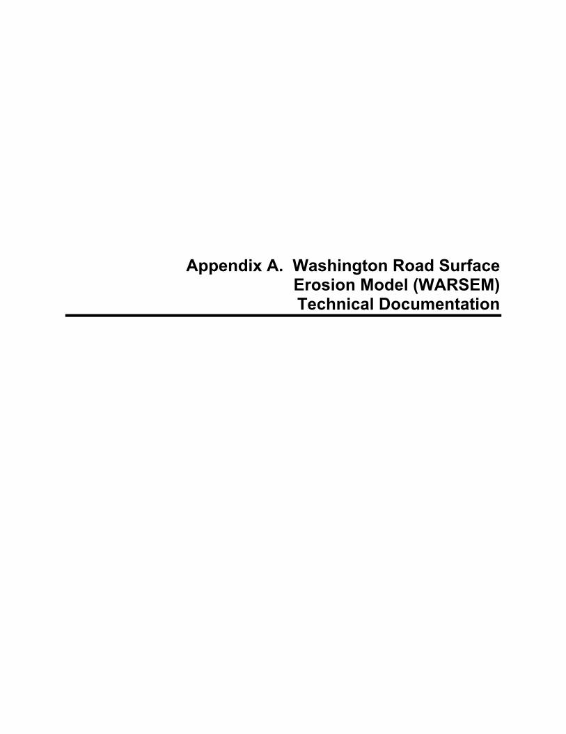
Appendix A. Washington Road Surface Erosion Model (WARSEM) Technical Documentation

Washington Road Surface Erosion Model Appendix A. Technical Documentation
Appendix A. Washington Road Surface Erosion Model Technical Documentation
Contents
A.1 Sediment Production from Road Surface Erosion .......................................................... A-3 A.2 Geologic Erosion Factor ................................................................................................. A-4 A.3 Tread Surfacing Factor ................................................................................................... A-6 A.4 Road Width and Traffic Factors ..................................................................................... A-8 A.5 Road Slope Factor......................................................................................................... A-12 A.6 Cutslope Height ............................................................................................................ A-12 A.7 Cutslope Cover Factor .................................................................................................. A-14 A.8 Rainfall Factor .............................................................................................................. A-16 A.9 Delivery Factor ............................................................................................................. A-18 A.10 Road Age Factor ........................................................................................................... A-21 A.11 Segment Length/Road Drainage Configuration............................................................ A-23 A.12 Special Considerations for Fillslopes............................................................................ A-24 A.13 Best Management Practices (BMPs) ............................................................................ A-24 A.14 References..................................................................................................................... A-25 List of Figures
Figure A-1. Geologic Erosion Rates Calculated from Road Erosion Measurements................ A-5 Figure A-2. Road Erosion Rates by Traffic Level................................................................... A-10 Figure A-3. Field-Averaged Cutslope Height versus Hillside Slope....................................... A-14 Figure A-4. Erosion Reduction on Cutslopes and Fillslopes with Varying Erosion Control
Treatments and Ground Cover.......................................................................................... A-15 Figure A-5. Predicted Erosion (WEPP) versus Average Annual Rainfall (PRISM)............... A-17 Figure A-6. Sediment Travel Distance Comparison................................................................ A-19 Figure A-7. Distribution of Total Eroded Sediment Volume Along Sediment Plume Downslope
of Cross Drains ................................................................................................................. A-20 Figure A-8. Time Trends in Erosion Following Road Construction. ...................................... A-22 Figure A-9. Generalized Runoff Flow Paths for Different Road Drainage Configurations. ... A-23 List of Tables
Table A-1. Geologic Erosion Factors. ....................................................................................... A-6 Table A-2. Road Surfacing Research......................................................................................... A-7 Table A-3. Road Tread Surfacing Factor................................................................................... A-8 Table A-4. Relative Sediment Production from Roads Normalized to Light Traffic Use ...... A-10 Table A-5. Road Width and Traffic Factors. ........................................................................... A-11 Table A-6. Road Slope Factor. ................................................................................................ A-12 Table A-7. Cutslope Height. .................................................................................................... A-13
Page A-1 February 20, 2004

Washington Road Surface Erosion Model Appendix A. Technical Documentation
Table A-8. Cutslope Cover Factor. .......................................................................................... A-16 Table A-9. Sediment Delivery/Distance Relationship (assuming total plume 350 feet long). A-21 Table A-10. Road Delivery Factors. ........................................................................................ A-21 Table A-11. Road Age Factor.................................................................................................. A-23 Table A-12. Segment Lengths/Widths Used for Different Road Drainage Configurations. ... A-24
List of Attachments
Attachment 1. Road Erosion Measurements used in Development of Geologic Erosion Factors
Page A-2 February 20, 2004

Washington Road Surface Erosion Model Appendix A. Technical Documentation
Appendix A. Washington Road Surface Erosion Model Technical Documentation
A.1 Sediment Production from Road Surface Erosion
Sediment is produced from four components of a standard forest road prism: the cutslope, ditch, tread, and fillslope. The amount of sediment produced from these components and delivered to streams is dependent upon the interaction of a multitude of variables, including rainfall intensity and timing; traffic and grading/maintenance activities; the type of surfacing on the road tread; cover (vegetation/rock) on the ditch, cutslope, and fillslope; the grain size, infiltration capacity, and cohesion of the underlying road material; interception of subsurface flow by the cutslope; gradient of the road and cut and fill slopes; snow accumulation and melt; the hydrologic function of slopes below the road; sediment transport on slopes below the road, length of roadway between drainage structures, shading on the roadway; and small-scale topographic features. While physical models such as WEPP for roads (http://forest.moscowfsl.wsu.edu/fswepp/) include some of these variables, it is presently not possible to model all of them, even on a small scale. It may be feasible to model all of these variables in the future, but it is unlikely that it will ever be practical to apply a detailed, physical model of road erosion over large areas using present technology. Given the limitations of the existing physical models and the fact that one of the goals of the Washington procedure is to be able to model large areas, Washington Road Surface Erosion Model utilizes empirical relationships linking road use, underlying geology, precipitation, road surfacing, road gradient, cutslope cover, road age, and distance from a stream approach to estimate average annual sediment supply to streams or other water bodies from surface erosion on forest roads, and uses several simplifying assumptions.
The model assumes that road segments that drain to the forest floor over 200 feet away from a stream or water body do not deliver sediment. This is based on studies of travel distances of sediment downslope of culvert outfalls by Trimble and Sartz (1957), Haupt (1959), Haupt and Kidd (1965), Swift (1985), Megahan and Ketcheson (1996), and Brake et al. (1997). These studies showed that the maximum distance sediment is carried downslope from culvert outlets or other types of cross drains is dependent upon the amount of water and sediment flowing through the cross drain, the gradient of the hillslope downhill from the outlet, and the number and type of obstructions (vegetation, downed logs) on the hillslope below the cross drain. However, the maximum travel distance in the studies was 30-550 feet, with sediment moving less than 150 feet in nearly all cases. It is also important to note that total sediment travel distance does not equate to total sediment delivery. Rather, the volume of sediment deposition decreases exponentially downslope in accordance with Stokes Law. This means that even if a water body is located closer than the total sediment travel distance for a site, only a fraction of the total sediment supplied from the road reaches the stream. For example, Megahan and Ketcheson (1996) show that only about 17% of the total volume of sediment travels beyond 50% of the total travel distance (see Figure A-7). This relationship was used to estimate the average volume of sediment delivery to streams for locations where cross drains are less than 200 feet from streams.
The model also assumes that sediment delivered to streams from fillslopes is negligible. This is based on measurements by Meghan and Ketcheson (1996) showing the mean travel distance of
Page A-3 February 20, 2004

Washington Road Surface Erosion Model Appendix A. Technical Documentation
fillslope sediments was 20 feet downslope of the fillslope, and field observations of nearly 100 percent cover on fillslopes on established roads (Dubé, unpublished data). These combined circumstances result in a negligible contribution of fillslope sediment to streams in most cases. There may be a few locations in a watershed, such as where a road closely parallels a stream for a long distance, or some unvegetated fillslopes at new road crossings where this assumption is not valid; these cases should be considered separately (see Section A.12).
The model also groups erosion from the tread and ditch together, so assigned road widths described below include both the running surface and ditch widths. The result of this assumption is to apply surfacing and traffic factors to the ditch as well as the tread. These two factors will tend to even each other out since most heavily used roads (high traffic factor) generally have gravel surfacing (lower surfacing factor). Very heavily used gravel roads (main haul roads) will have a very high traffic factor, but applying this to the ditch is probably appropriate since these roads and ditches are likely regraded frequently, disturbing the ditch’s armor layer and increasing sediment production.
The average annual volume of sediment delivered to a stream from each road segment is calculated based on the following formulas:
Total Sediment Delivered to a Stream from each Road Segment (in tons/year) = (Tread & Ditch + Cutslope) x Road Age Factor Eq. 1
Tread & Ditch = Geologic Erosion Factor x Tread Surfacing Factor x Traffic Factor x Segment Length x Road (Tread + Ditch) Width x Road Slope Factor x Rainfall Factor x Delivery Factor Eq. 2
Cutslope = Geologic Erosion Factor x Cutslope Cover Factor x Segment Length x Cutslope Height x Rainfall Factor x Delivery Factor Eq. 3
Values for each factor in the equations are assigned based on user input for each road segment as described below. Note that model results are very sensitive to some of the factors and less sensitive to others. An analysis of model sensitivity and recommendations for potential future study to improve our understanding of these variables is included in Appendix D.
A.2 Geologic Erosion Factor
The inherent erodibility of a particular road segment is determined by soil attributes where the road is constructed. Soil erodibility is affected by the soil particle size and cohesiveness, and the amount of runoff generated from a road that can erode and transport sediment depends upon the infiltration capacity of the soil (as well as rainfall patterns). Soils with a high silt content are most erodible; clay-dominated soils are less erodible, and soils with a high gravel component are least erodible (Goldman et al. 1986, Burroughs et al. 1992). Since most road prisms in mountainous areas are graded into the sub-soil, erodibility is a factor of parent material (geology) and degree of weathering rather than surface soil properties.
Page A-4 February 20, 2004

Washington Road Surface Erosion Model Appendix A. Technical Documentation
Road erosion measurements from a variety of locations, lithologies, and climatic zones were compiled to provide insight into the Geologic Erosion Factor (Bilby et al. 1989, Dryness 1975, Foltz 1996, Luce and Black 1999a, Ketcheson and Megahan 1996, Kochenderfer and Helvey 1984, Megahan and Kidd 1972a, Megahan et al. 1986, Paulson 1997, Reid 1981, Reid and Dunne 1984, Swift 1984, Toth 2000, Vincent 1985, Wald 1975; see Attachment 1). The annual sediment yield from each study (in tons/acre/yr) was normalized to a reference condition by dividing by the appropriate estimated Rainfall Factor, Traffic Factor, Surfacing Factor, and Road Slope Factor. The resulting value is the Geologic Erosion Factor that would be required in model calculations to obtain the measured erosion rate. An average Geologic Erosion Factor was calculated for each study, and then for each geology (Figure A-1).
Figure A-1. Geologic Erosion Rates Calculated from Road Erosion Measurements.
0
5
10
15
20
25
30
35
40
45
basal
t
granit
egra
vel
metamorp
hic
sandst
one
schist
OR sedim
entar
y
SE US se
dimen
tary
WA se
dimen
tary
tuff
Geo
logi
c Er
osio
n R
ate
(tons
/ac/
yr)
Dark circles are average value for each rock or sediment type; boxes show 25th and 75th percentile values, and bars show maximum and minimum values for geology. Based on values shown in Attachment 1.
The road erosion measurements from most lithologies result in a Geologic Erosion Factor of close to 1, suggesting that the erosion rates, combined with the traffic, surfacing, and road slope factors, adequately predict erosion for most competent rock types. However, road erosion from the granitic, schist, and deeply weathered sedimentary rocks is 4 to 15 times greater than predicted. The values for the roads on granitic soils were primarily measured from newly constructed roads. A road age factor of 4 was used for all these values since the specific road age was not always available. As a result, these values are likely 2 to 3 times higher than the
Page A-5 February 20, 2004

Washington Road Surface Erosion Model Appendix A. Technical Documentation
model would predict for a 1-year old road. Based on Figure A-1 and studies of relative erodibility between different rock types (André and Anderson 1961, Burroughs et al. 1992, Reinig et al. 1991, WDNR 1997), the Geologic Erosion Factors in Table A-1 were established for the model.
Table A-1. Geologic Erosion Factors. WARSEM uses Geologic Erosion Factors of Low (1), Moderate (2) or High (5)
Geologic Age of Formation1 Lithology Quaternary Tertiary Mesozoic Paleozoic Precambrianun-weathered metamorphic rocks - 1 1 1 1
weathered schist or gneiss - 2 2 2 2 basalt 1 1 1 1 1 andesite 1 1 1 1 1 ash 5 5 1 1 1 tuff 5 5 1 1 1 un-weathered intrusive rocks - 1 1 1 1 weathered granite/intrusive rocks - 5 5 5 5
un-weathered/ hard sedimentary rocks - 1 1 1 1
coarse-grained soft sediments (gravelly) 1 1 - - -
fine-grained or deeply weathered sediments (silt, sand)
5 5 - - -
1 Some lithology/ages categories do not have geologic erosion rates because these categories do not occur (e.g., there are no Quaternary metamorphic rocks present on the earth’s surface). The Geologic Erosion Factor is selected for each road segment from the geology field input into the model. Geologic Erosion Factors are entered as Low (1), Moderate (2) or High (5). The default geology coverage is based on the 1:500,000 scale geologic map of Washington (Huntting et al. 1961) and keyed to the Township/Range/Section entered for each road segment. Geologic erosion factors for each geologic unit on the map were assigned based on dominant lithology and age as shown in Table A-1. If the user identifies their own, site-specific Geologic Erosion Factor for rock types in their study area, the factors should be based on Table A-1 since these rates are scaled to the precipitation and traffic factors the model uses.
A.3 Tread Surfacing Factor
The type and quality of surfacing on a road has a large effect on how well the road holds up to traffic use. The surface of native (unsurfaced) roads, particularly those constructed on erodible soils, are easily broken into fine particles that are subsequently subject to surface erosion. Native roads also often form ruts, especially if used during wet conditions which further increase
Page A-6 February 20, 2004
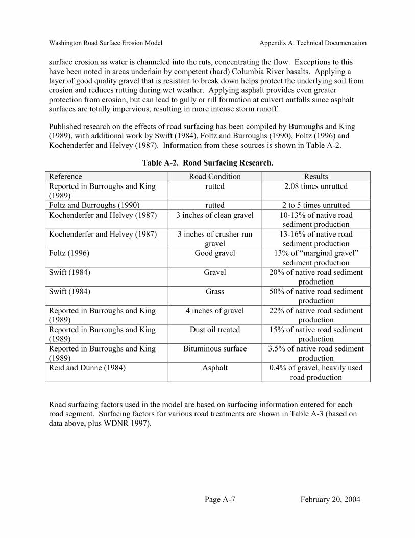
Washington Road Surface Erosion Model Appendix A. Technical Documentation
surface erosion as water is channeled into the ruts, concentrating the flow. Exceptions to this have been noted in areas underlain by competent (hard) Columbia River basalts. Applying a layer of good quality gravel that is resistant to break down helps protect the underlying soil from erosion and reduces rutting during wet weather. Applying asphalt provides even greater protection from erosion, but can lead to gully or rill formation at culvert outfalls since asphalt surfaces are totally impervious, resulting in more intense storm runoff.
Published research on the effects of road surfacing has been compiled by Burroughs and King (1989), with additional work by Swift (1984), Foltz and Burroughs (1990), Foltz (1996) and Kochenderfer and Helvey (1987). Information from these sources is shown in Table A-2.
Table A-2. Road Surfacing Research.
Reference Road Condition Results Reported in Burroughs and King (1989)
rutted 2.08 times unrutted
Foltz and Burroughs (1990) rutted 2 to 5 times unrutted Kochenderfer and Helvey (1987) 3 inches of clean gravel 10-13% of native road
sediment production Kochenderfer and Helvey (1987) 3 inches of crusher run
gravel 13-16% of native road sediment production
Foltz (1996) Good gravel 13% of “marginal gravel” sediment production
Swift (1984) Gravel 20% of native road sediment production
Swift (1984) Grass 50% of native road sediment production
Reported in Burroughs and King (1989)
4 inches of gravel 22% of native road sediment production
Reported in Burroughs and King (1989)
Dust oil treated 15% of native road sediment production
Reported in Burroughs and King (1989)
Bituminous surface 3.5% of native road sediment production
Reid and Dunne (1984) Asphalt 0.4% of gravel, heavily used road production
Road surfacing factors used in the model are based on surfacing information entered for each road segment. Surfacing factors for various road treatments are shown in Table A-3 (based on data above, plus WDNR 1997).
Page A-7 February 20, 2004
Washington Road Surface Erosion Model Appendix A. Technical Documentation
Table A-3. Road Tread Surfacing Factor.
Surface Type Surfacing Factor Asphalt 0.03 Gravel 0.2 Gravel with Ruts 0.4 Pitrun or Worn Gravel 0.5 Grassed Native 0.5 Native Surface 1 Native with Ruts 2
An asphalt surface refers to one that has a permanent bituminous surface. A gravel surface refers to a road with a layer of competent gravel; the gravel particles should cover the surface with few fine-grained particles visible on the road surface. Pitrun or worn gravel refers to a road tread that has been covered with pitrun gravel (unsorted product of the crushing process – has lots of fine particles as well as gravel) or gravel that has been broken down by traffic and is mixed with abundant fine-grained material.
There are a variety of other road surface treatments, such as chipseal, dust reduction products, or oil that may be applied to road surfaces in a particular area. These may be entered as a Best Management Practice (BMP - see Appendix C). Few studies were found to document sediment reduction resulting from these measures. Standard BMPs number 1 through 7 refer to some of these practices.
A.4 Road Width and Traffic Factors
The width of the road tread and the amount of traffic on a road both influence the amount of surface erosion produced from the road tread. Often the width and traffic levels are closely associated in a road network: mainline roads are usually wider to accommodate the heavy traffic levels and allow vehicles to pass without using pullouts; spur roads are much narrower since they receive minimal or sporadic traffic. The road surface erosion model allows the user to enter segment-specific traffic and width values, or to use defaults based on road class.
Over time, the surface of a roadway will develop an armor layer of larger particles that are resistant to erosion as runoff removes the smaller, easily erodible particles. This armor layer develops fairly quickly, and remains as long as the road surface is not disturbed. Vehicles driving over the road or grading of the roadway disrupt this armor layer, breaking down the larger surface particles by crushing and abrasion, and bringing small particles from below the surface layer to the surface of the road. The effects of traffic can be seen quite clearly by driving on an un-used forest road during a rainstorm. Road runoff is clear until just a single pass with a vehicle disrupts the surface and results in muddy runoff behind the vehicle. Traffic during precipitation or runoff events results in continuous disruption of the road surface with consequent high erosion rates. Traffic during dry weather breaks down the road surface into smaller particles that are carried away during the next runoff event, but if the traffic is discontinued during wet weather, the road surface quickly armors and limits further erosion.
Page A-8 February 20, 2004

Washington Road Surface Erosion Model Appendix A. Technical Documentation
There have been several studies of the effects of traffic levels on surface erosion in different parts of the country. Early studies noted large increases in suspended sediment loads leaving roadways that were actively used by truck traffic. Wald (1975) noted roads used by log trucks generated 13 times more sediment than a control (no traffic). He also noted runoff following grading of the road had 3.6 times as much sediment as prior to grading. Wooldridge (1979, Figure 7) found increased sediment levels in streams below forest roads during work days with precipitation, but no increased levels of suspended sediment in the creek on the following weekend day (no traffic) despite heavier rainfall.
Research by Reid (1981), Reid and Dunne (1984), Sullivan and Duncan (1981), and Foltz (1996) was specifically aimed at determining the effects of traffic on road erosion. The Reid and Sullivan and Duncan studies sampled suspended sediment concentrations in road runoff and extrapolated the results over storm hydrographs and then to an entire year. Reid’s work was done in the Clearwater River watershed on the Olympic peninsula (average 153 inches of rain/year during study), on worn gravel roads underlain by Tertiary sedimentary rocks. Sullivan and Duncan’s study area was the Deschutes and Chehalis River watersheds, gravel roads underlain by glacial outwash and basalt, respectively. Average annual precipitation is 51 inches in the Deschutes basin and 110 inches in the Chehalis basin. Traffic rates in the studies included heavy mainline roads (over 4 log trucks/day), moderate use (1-3 trucks/day), light administrative use (<1 log truck plus pickup traffic) to abandoned/inactive (blocked) roads with no use. In addition, Reid collected data from heavily used roads during temporary non-use periods when log trucks were not running.
Erosion rates reported in the 3 studies were normalized to tons/acre/inch of rainfall, and related to the average number of log trucks/day (Figure A-2). All studies showed increasing erosion rates with increased traffic use. Variations in the rates of erosion between studies are likely caused by other factors such as gravel quality, as seen by the difference in erosion rates between the 2 surfacing types in the Foltz study (good quality gravel and pitrun marginal quality gravel).
Page A-9 February 20, 2004

Washington Road Surface Erosion Model Appendix A. Technical Documentation
Figure A-2. Road Erosion Rates by Traffic Level
0
2
4
6
8
10
12
0 1 2 3 4 5
Average log truck loads/day
Eros
ion
Rat
e (to
ns/a
cre/
inch
pre
cipi
tatio
n)
Foltz pitrun Foltz gravel Reid and Dunne Sullivan & Duncan
temporary non-use
In order to factor out all other sources of variability, the erosion rates in tons/acre/inch of precipitation were normalized by dividing by the erosion rate for the “reference” light traffic road segment in each of the studies. The results of these calculations, shown in Table A-4, show somewhat similar values across use categories, but still have variability between study sites.
Table A-4. Relative Sediment Production from Roads Normalized to Light Traffic Use
Use Rate Foltz gravel
Foltz pitrun
Reid and Dunne worn gravel
Sullivan and
Duncan
Heavy (>4 loads/day) - - 125 46 Mod. Heavy (3-4 loads/day) 9 12 - - Moderate (2 loads/day) 2 8 10 - Light (<1 load/day) 1 1 1 1 Abandoned (Inactive) - - 0.13 - Temporary Non Use (weekend) - - 16 -
Page A-10 February 20, 2004

Washington Road Surface Erosion Model Appendix A. Technical Documentation
Road width and traffic factors used in the model are based on the road class or width and traffic level assigned to each road segment. The user can opt to assign road classes to road segments, in which case the default width and traffic factors shown in Table A-5 will be used, or the user can enter measured width and traffic levels separately. Traffic factors in Table A-5 are based on the information presented in Table A-4. Road widths include both the running surface (tread) and ditch widths. The default width values are based on average measurements taken by K. Dubé during road erosion inventories on road segments that drain to streams at over 800 road segments in watersheds in Washington, Oregon, and Idaho (Boise Cascade Corporation, unpublished data). These measurements were made on private, state, and federal lands as part of road erosion surveys during watershed analyses conducted by Boise Cascade Corporation.
Table A-5. Road Width and Traffic Factors.
Average passes/day
Road Width
Road Class Description Log Truck
Pickup/ car
Traffic Category
Traffic Factor
(tread & ditch
in ft) Highway Very heavy use by truck and car
traffic throughout the year. If surface is paved, see note below*.
>5 >5 Heavy 120 40
Main Haul Heavily used by log truck traffic throughout the year; usually the main access road in a watershed that is being actively logged.
4-5 >5 Mod. Heavy 50 30
County Road
Wide, county-maintained road that receives heavy residential and/or log truck use.
3-5 >10 Mod. Heavy 50 35
Primary Road
Receives moderate use by log trucks throughout all or most of the year. Usually roads branching off main haul road that head up tributaries or that access large portions of the watershed.
3-4 5-10 Moderate 10 25
Secondary Road
Receives light log truck use during the year. May occasionally be heavily used to access a timber sale. Receives car/pickup or recreational use.
1-2 1-5 Light 2 18
Spur Road Short road used to access a logging unit. Used to haul logs for a brief time while unit is logged. On the average receives little use.
<1 <1 Occ-asional 1 15
Abandoned inactive or
blocked
Road is blocked by a tank trap, boulders, etc. or is no longer used by traffic.
0 0 None 0.1 15
* Note: if road traffic levels are classified as “Heavy” and the surface is asphalt, check to make sure the results are reasonable. There will be little erosion from the paved surface, but the increased runoff could result in ditch erosion.
Page A-11 February 20, 2004
Washington Road Surface Erosion Model Appendix A. Technical Documentation
In order to determine which is the most appropriate traffic factor to assign to a segment, select the road use category that most closely fits each road type in your road file. Average traffic use for both log truck traffic and residential/recreational/administrative traffic (vehicles/day) is provided as a guideline. The average vehicles/day values in Table A-5 were based on traffic use averaged over all days in a year (including weekends and non-use periods). To determine the appropriate average use category, determine total trips/year on a road and divide by 365 days. Use of specific roads by log trucks changes over time as timber sales occur in different parts of a watershed. To determine average road erosion in the watershed, pick the long-term average traffic rates for each road type. To determine sediment input from a specific timber sale, select use rates that best fit the traffic rates on that road during the sale. To model seasonal changes in traffic patterns, (such as summer use only, or only winter haul on snow-covered roads) set up a custom BMP. This procedure, described in Appendix C (Section C.8), allows the user to enter a specific traffic level for each month of the year.
A.5 Road Slope Factor
The gradient, or slope, of a road segment influences the erosion rate. Water flows more quickly down steeper road segments, resulting in more erosive power (higher shear stress). Luce and Black (1999a) found that amount of erosion varied with the product of the segment length times road slope squared. A similar factor was used by Reinig et al (1991) in their formulation of road surface erosion calculations.
The model assigns a road slope factor to each road segment based on the road tread slope category entered by the user. The road slope factor is based on the formula:
2
%5.7Slope(%) Tread RoadFactor Slope Road
= Eq. 4
with a reference slope of 7.5 percent. The reference slope of 7.5 percent was selected as the average slope of the 5-10 percent slope category. Factors used are shown in Table A-6.
Table A-6. Road Slope Factor.
Road Tread Slope Slope Factor < 5 percent 0.2 5-10 percent 1.0 > 10 percent 2.5
A.6 Cutslope Height
Few studies have been performed evaluating the differences in sediment production based solely on the height of cutslopes. Luce and Black (1999b) reported only a slight correlation between sediment production from a road and cutslope height, and Megahan et al. (2001) found no correlation. Both of these studies included multiple variables in their analysis, and concluded that either the cutslope height variable was overshadowed by the changes in other variables studied, or was not dependent upon cutslope height because taller cutslopes are cut into the C
Page A-12 February 20, 2004

Washington Road Surface Erosion Model Appendix A. Technical Documentation
soil horizons, which are often less erodible than the overlying A and B horizons. The results of these 2 studies are somewhat at odds with conventional erosion calculations, and measurements on other plot studies that have resulted in equations relating soil erosion to a length-slope factor (e.g., the Universal Soil Loss Equation, and the Water Erosion Prediction Project (WEPP) model). However, conventional studies all dealt with surface soil materials whereas road cutslope erosion includes parent materials, especially on steeper slopes.
The Washington Road Surface Erosion Model uses the cutslope height factor (measured as slope length) to determine the area of the cutslope (when multiplied by segment length). If the user is measuring cutslope height in the field, the average cutslope height (averaged over entire segment length) is recorded to the nearest category: no cutslope; 2.5 feet; 5 feet; 10 feet; or 25 feet. A default cutslope height value of 5 feet is assigned by the model unless the user enters a specific cutslope height.
Road segments that are imported from the SEDMODL program have pre-assigned cutslope heights based on hillside gradient. The SEDMODL program calculates hillside gradient and groups it into one of 4 categories. Cutslope height for each gradient category (Table A-7) is based on the average of cutslope heights measured during road erosion inventories, displayed on Figure A-3. The field measurements were mean cutslope height over the length of road that drained to the stream. These averaged heights may be lower than expected because they take into account the low (or non-existent) cutslope height close to a stream crossing.
Table A-7. Cutslope Heights assigned by SEDMODL2.
Hillside Gradient Cutslope Height (ft) 0-15 percent 2.5 15-30 percent 5 30-60 percent 10 > 60 percent 25
Page A-13 February 20, 2004

Washington Road Surface Erosion Model Appendix A. Technical Documentation
Figure A-3. Field-Averaged Cutslope Height versus Hillside Slope
0
5
10
15
20
25
30
35
40
0 10 20 30 40 50 60 70 80 90Hillside Slope (%)
Hei
ght (
ft)average=2.5 ft 5 ft 25 ft10 ft
Based on unpublished field measurements taken during road Boise Cascade inventories in Washington, Idaho, and
Oregon
A.7 Cutslope Cover Factor
The amount of vegetation, rock cover, or armoring on a cutslope has a large effect on whether or not underlying soil particles are detached by rainfall or dry ravel. A large amount of research has been completed on the effects of cover on erosion rates, often in conjunction with erosion control measures that are applied to freshly constructed cut and fill slopes. An excellent compilation of past studies is included in Burroughs and King (1989). Recent research has also been reported by Megahan et al. (1992), Megahan et al. (2001) and Grace (2002). On-going research on the effectiveness of commercial erosion control products, including vegetative cover and erosion reduction following a growing season, is reported at the Texas Department of Transportation web site (2002 publication: ftp://ftp.dot.state.tx.us/pub/txdot-info/mnt/erosion/2001cycle.pdf).
The relative effectiveness of ground cover at reducing erosion on cutslopes is a function of not only the percent of ground that is protected, but if the cover is in contact with the ground surface and root strength (live grass in the Grace study was generally very effective at reducing erosion). The cover/erosion reduction relationship chosen for the current model closely mimics that used in the WDNR Watershed Analysis procedures (WDNR 1997). The curve used in the WARSEM calculations, shown as the bold black line on Figure A-4, is close to the “Wood chips/rock” relationship reported in Burroughs and King, and is appropriate for cutslope on most established roads that have been left to armor and revegetate naturally, resulting in a mix of rocks, debris, and vegetation. For cutslopes that have been recently treated with an erosion control product, it
Page A-14 February 20, 2004
Washington Road Surface Erosion Model Appendix A. Technical Documentation
may be more appropriate to use an alternative erosion reduction ratio, as described in Appendix C (BMPs).
Figure A-4. Erosion Reduction on Cutslopes and Fillslopes with Varying Erosion Control Treatments and Ground Cover.
0%
10%
20%
30%
40%
50%
60%
70%
80%
90%
100%
0 20 40 60 80 100
Ground Cover (%)
Perc
ent E
rosi
on R
educ
tion
Native GrassExotic GrassErosion MatStrawStraw with netStraw/Asphalt tackErosion MatWood chips/rockHydromulchWDNR (1997)Current Model
(data with thin solid lines from Burroughs and King (1989); data with solid points and no line from Grace (1999); bold solid line shows erosion reduction used in current model)
The model assigns a Cutslope Cover Factor based on the percent vegetation or rock cover the user enters. There are three methods to specify cutslope cover: (1) model default value; (2) user specifies a single cover value for the entire watershed; and (3) user enters cutslope cover attribute for each road segment.
The model uses a default value of 70 percent vegetative and/or rock cover on cutslopes. The 70 percent cover value was the average of cutslope cover during the road erosion inventories (Boise Cascade Corporation, unpublished data). Table A-8 lists cover factors the model uses if other percent cover values are specified by the user.
Page A-15 February 20, 2004

Washington Road Surface Erosion Model Appendix A. Technical Documentation
Table A-8. Cutslope Cover Factor.
Percent Vegetation or Rock Cover
Cover Factor
90-100 0.1023 70-90 0.2014 50-70 0.3133 30-50 0.4466 10-30 0.6359 0-10 0.8850
A.8 Rainfall Factor
Rainfall and snowmelt are the dominant erosion and transport mechanisms affecting road surface erosion in most areas of Washington. Falling raindrops can dislodge sediment particles, and runoff from rainstorms or snowmelt can entrain and transport particles. The true amount of erosion and transport resulting from rainfall and snowmelt depends upon a complex interaction of the factors causing increased energy available for erosion and transport (raindrop size and intensity, rate of snowmelt, infiltration capacity of roadway) in conjunction with the availability of loose or easily erodible particles on the road surface (grain size of sediment, traffic and grading during rainfall or snowmelt to keep a supply of loosened particles). Since many of these factors are highly variable through time, it is not possible to quantify them precisely in the current, time-averaged empirical model. Instead, a simplified rainfall factor is used to capture the essential elements of the precipitation-erosion relationship.
The Version 4.0 WDNR surface erosion module (WDNR 1997) used a precipitation factor that was based on average annual total precipitation (rain plus snow). However, studies of road erosion have shown that road erosion resulting from snowmelt runoff is an order of magnitude lower than from the equivalent amount of rain runoff (Vincent 1985). This likely resulted in an overestimate of erosion at higher elevations, where much of the total precipitation falls as snow. The rainfall factor in the present model is based on average annual rainfall amount, corrected for snowmelt, as described below.
A few road erosion studies have measured erosion from the same road segments over several years with a range of precipitation values (Luce and Black 1999a, Swift 1984). Best-fit power functions to data from these two studies yields equations of the form:
Erosion = a [Rainfall]2 Eq. 5
However, the range of precipitation values in the data sets was limited, with a range from 35-70 inches in the Swift study and 60-80 in the Luce and Black study.
In order to determine if the above relationship was valid over a wider climatic range, the Water Erosion Prediction Project (WEPP) model was used to estimate road surface erosion (Elliot et al. 1999). The WEPP:Road interface was used to calculate road erosion from a standard road
Page A-16 February 20, 2004

Washington Road Surface Erosion Model Appendix A. Technical Documentation
configuration over a wide variety of climatic stations (74 different locations) in Washington, Oregon, Idaho, California, and Montana. The standard road configuration used was an insloped, 4% gradient, native-surfaced, 200-foot long, 15-foot wide road. The four standard WEPP soil types (silt loam, sandy loam, clay loam, and loam) were run for each climate.
The average annual rainfall at each of the 74 test sites was calculated using average monthly total precipitation and average monthly snowfall amounts from the PRISM climatic model (http://www.ocs.orst.edu/prism/prism_new.html). The PRISM data sets are based on average 1961-1990 climatic data, and cover the entire United States at a 2 km resolution. Average annual rainfall was calculated by subtracting the average monthly snow water equivalent from the average monthly precipitation at each location using the formula:
Average annual rainfall = Σ [(January precipitation – 0.1 x January snowfall) + (February precipitation – 0.1 x February snowfall) + …………………+ (December precipitation – 0.1 x December snowfall)] Eq. 6
A 10% snow water equivalent (0.1 factor in Equation 6) was used to transform the monthly snowfall amounts to equivalent rainfall amounts. The actual snow water equivalent of freshly fallen snow ranges from 0.05 at air temperatures of 14°F to 0.20 at temperatures at 32°F (Natural Resource Conservation Service). Using a single value of 0.1 for all months and elevations is a simplification, and likely results in somewhat of an overestimate of the amount of rainfall each month, particularly in warmer and wetter areas of the west-side Cascades and Olympics. This would result in a higher rainfall factor, and predict a higher erosion rate at these locations. However, snow in these same areas is more likely to be transient, and subject to rain-on-snow events that result in more rapid melting of the accumulated snow pack, resulting in greater erosion than would occur from a more gradual seasonal melting of the snowpack, so the slight overestimate of predicted erosion is not unreasonable.
Figure A-5 shows the results of the WEPP run for each climate station, with predicted erosion plotted against the total rainfall from the PRISM data.
The WEPP results follow a similar power function form as the Swift and Luce and Black data sets, but over the much wider climatic range. The exponent based on the WEPP data for clay, silt, and loam soils is 1.3 to 1.4, with an exponent of 1.9 for sandy soils. The exponent for all soil types combined is 1.5. The relationship for all soil types combined was used to obtain the rainfall factor for the model.
A Rainfall Factor is assigned for each road segment based on the location (Township/Range Section) the user enters into the model. The factor was derived based on the average annual rainfall for that T/R Sec. (from the PRISM data) and the following formula:
Rain Factor = 0.016 [Average Annual Rainfall (inches)]1.5 Eq. 7
Page A-17 February 20, 2004
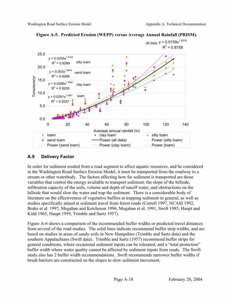
Washington Road Surface Erosion Model Appendix A. Technical Documentation
Figure A-5. Predicted Erosion (WEPP) versus Average Annual Rainfall (PRISM). y = 0.0159x1.5016
R2 = 0.8758
y = 0.0255x1.4164
R2 = 0.9289
y = 0.003x1.8916
R2 = 0.9289
y = 0.0289x1.3364
R2 = 0.9205
y = 0.0291x1.3581
R2 = 0.9257
0.0
5.0
10.0
15.0
20.0
25.0
0 20 40 60 80 100 120 1Average annual rainfall (in)
Tons
/acr
e/yr
40
loam clay loam silty loamsand loam Power (all data) Power (silty loam)Power (sand loam) Power (clay loam) Power (loam)
all data:
silty loam
sand loam
clay loam
loam
A.9 Delivery Factor
In order for sediment eroded from a road segment to affect aquatic resources, and be considered in the Washington Road Surface Erosion Model, it must be transported from the roadway to a stream or other waterbody. The factors affecting how far sediment is transported are those variables that control the energy available to transport sediment: the slope of the hillside, infiltration capacity of the soils, volume and depth of runoff water, and obstructions on the hillside that would slow the water and trap the sediment. There is a considerable body of literature on the effectiveness of vegetative buffers at trapping sediment in general, as well as studies specifically aimed at sediment travel from forest roads (Correll 1997, NCASI 1992, Brake et al. 1997, Megahan and Ketcheson 1996, Megahan et al. 1991, Swift 1985, Haupt and Kidd 1965, Haupt 1959, Trimble and Sartz 1957).
Figure A-6 shows a comparison of the recommended buffer widths or predicted travel distances from several of the road studies. The solid lines indicate recommend buffer strip widths, and are based on studies in areas of sandy soils in New Hampshire (Trimble and Sartz data) and the southern Appalachians (Swift data). Trimble and Sartz (1957) recommend buffer strips for general conditions, where occasional sediment inputs can be tolerated, and a “total protection” buffer width where water quality cannot be affected by sediment inputs from roads. The Swift study also has 2 buffer width recommendations. Swift recommends narrower buffer widths if brush barriers are constructed on the slopes to slow sediment movement.
Page A-18 February 20, 2004

Washington Road Surface Erosion Model Appendix A. Technical Documentation
Figure A-6. Sediment Travel Distance Comparison
0
50
100
150
200
250
300
350
0 10 20 30 40 50 60 70 8
Hillslope Gradient
Rec
omm
ende
d B
uffe
r or P
redi
cted
Tra
vel D
ista
nce
(ft)
0
Swift Swift w/brush barriers Trimble&SartzTrimble&Sartz total protection Megahan & Ketcheson Brake
The dashed lines in Figure A-6 indicate maximum transport distances (end of the sediment plume) predicted by regression equations developed by Megahan and Ketcheson (1996) and Brake et al. (1997) using mean values for all variables except slope. The Megahan and Ketcheson regression is based on a study of sediment travel distances below road culverts constructed in sandy soils in central Idaho. The Megahan and Ketcheson results are similar to previous studies in central Idaho by Haupt (1959) which showed most sediment travel distances to be less than 200 feet, but a few locations where sediment traveled over 300 feet. The Brake data comes from a study in the Oregon Coast range, and included coarse- and fine-grained soils (Brake et al. 1997). The travel distances in the study by Brake et al. seem anomalously short compared to other studies but very heavy brush cover in the area probably contributes to the reduced sediment travel distances.
The data in Figure A-6 indicate the maximum travel distance observed, that is the farthest distance that particles were found from the road culvert. Sediment downslope of a culvert is distributed in a depositional plume between the culvert and the end of the deposition area. Ketcheson and Megahan (1996) measured the distribution of sediment along sediment plumes, and found that most sediment was deposited close to the culvert, with an exponentially declining amount of sediment farther downslope (Figure A-7).
Page A-19 February 20, 2004

Washington Road Surface Erosion Model Appendix A. Technical Documentation
Figure A-7. Distribution of Total Eroded Sediment Volume Along Sediment Plume Downslope of Cross Drains
From Ketcheson and Megahan (1996)
The information in Figure A-6 on maximum travel distances, along with the distribution in Figure A-7 were combined to estimate the sediment delivery factors used in the road surface erosion model. A maximum plume length (sediment travel distance) of 350 feet was assumed, based on the data from Megahan and Ketcheson and Trimble and Sartz. This is a maximizing assumption; it is likely that nearly all sediment plumes will be less than 350 feet, but given the number of variables required to predict actual travel distance, plus the variability in the data, it was not considered feasible to make site-specific predictions of delivery. Given a plume length of 350 feet, Table A-9 shows the percent of the total sediment exiting the culvert that is transported past a given distance down the plume. This relationship can be used to estimate what percent of the total road sediment reaches a stream that is a given distance from the culvert. For example, if a stream is located 35 feet from the culvert, 70% of the total sediment leaving the culvert would be delivered to the stream (the remaining 30% of the sediment would be deposited between the culvert and the stream).
Page A-20 February 20, 2004
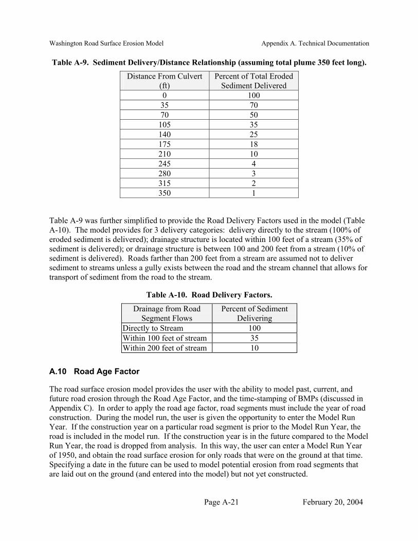
Washington Road Surface Erosion Model Appendix A. Technical Documentation
Table A-9. Sediment Delivery/Distance Relationship (assuming total plume 350 feet long).
Distance From Culvert (ft)
Percent of Total Eroded Sediment Delivered
0 100 35 70 70 50 105 35 140 25 175 18 210 10 245 4 280 3 315 2 350 1
Table A-9 was further simplified to provide the Road Delivery Factors used in the model (Table A-10). The model provides for 3 delivery categories: delivery directly to the stream (100% of eroded sediment is delivered); drainage structure is located within 100 feet of a stream (35% of sediment is delivered); or drainage structure is between 100 and 200 feet from a stream (10% of sediment is delivered). Roads farther than 200 feet from a stream are assumed not to deliver sediment to streams unless a gully exists between the road and the stream channel that allows for transport of sediment from the road to the stream.
Table A-10. Road Delivery Factors.
Drainage from Road Segment Flows
Percent of Sediment Delivering
Directly to Stream 100 Within 100 feet of stream 35 Within 200 feet of stream 10
A.10 Road Age Factor
The road surface erosion model provides the user with the ability to model past, current, and future road erosion through the Road Age Factor, and the time-stamping of BMPs (discussed in Appendix C). In order to apply the road age factor, road segments must include the year of road construction. During the model run, the user is given the opportunity to enter the Model Run Year. If the construction year on a particular road segment is prior to the Model Run Year, the road is included in the model run. If the construction year is in the future compared to the Model Run Year, the road is dropped from analysis. In this way, the user can enter a Model Run Year of 1950, and obtain the road surface erosion for only roads that were on the ground at that time. Specifying a date in the future can be used to model potential erosion from road segments that are laid out on the ground (and entered into the model) but not yet constructed.
Page A-21 February 20, 2004

Washington Road Surface Erosion Model Appendix A. Technical Documentation
The road construction year is also used to increase the sediment production from “new” road segments, those less than 2 years old. Research on road erosion has shown that new or rebuilt roads have a much higher erosion rate during the first 1-2 years following construction than in subsequent years (Ketcheson et. al 1999, Luce and Black 1999a, Grace 1999, Swift 1984, Dryness 1975, Megahan 1974, Megahan and Kidd 1972b). The majority of erosion from new roads comes from fillslopes, cutslopes, and ditches until these areas revegetate and/or armor. Monitoring of recovery following construction shows an exponential decline in erosion rates (Figure A-8). When compared to the long-term road erosion rate, the first year following construction yields approximately 10 times the long-term rate, the second year yields twice the long-term rate, and subsequent years are at the long-term rate. These factors, shown in Table A-11, are used in model run if road segments have been coded with construction year.
Figure A-8. Time Trends in Erosion Following Road Construction.
0
2
4
6
8
10
12
14
1 2 3 4 5 6
Time after Construction (Years)
Rel
ativ
e Se
dim
ent P
rodu
ctio
n
Ketcheson et al. (1999) Ketcheson et al. (1999) Luce and Black (1999)
Dryess (1975) Megahan and Kidd (1972)
Erosion from unprotected fillslopes on newly constructed roads can be a source of sediment to streams. The WARSEM calculations do not include sediment from fillslopes. If the area you are modeling has a large number of unvegetated fillslopes, you may want to consider adding sediment from these sources. Section A.12 describes one way to do this within the limitation of the model.
Erosion control measures on newly constructed roads and/or sediment retention measures have been shown to effectively reduce sediment loss from fresh road cutslopes and fillslopes
Page A-22 February 20, 2004

Washington Road Surface Erosion Model Appendix A. Technical Documentation
(Burroughs and King 1989, Megahan 1991, Megahan et al. 1992, 2001). If the new roads in your watershed have effective erosion control measures, it is important to include these as BMPs, as described in Appendix C. Otherwise, the modeled erosion rates may be too high for the initial 2 years.
Table A-11. Road Age Factor.
Road Age (Model Run Year minus
Construction Year) Road Age
Factor 0-1 10 2 2
>2 or no construction year specified 1
A.11 Segment Length/Road Drainage Configuration
The road drainage configuration (insloped/outsloped/crowned) determines the flow path of water and sediment from each portion of the road prism (Figure A-9).
F ths for Different Road Drainage Configurations. igure A-9. Generalized Runoff Flow Pa
Insloped with ditch Outsloped
Crowned
The user can ente rainage conf
r all roads in the model run. Segment lengths and widths used for calculations are shown in
Outsloped with wheel tracks (modeled as insloped)
r the road d iguration for each road segment, or use a single value foTable A-12. A 50 foot length of delivering tread/cutslope was chosen for outsloped roads. Thiswas the length of road prism generally found to be close enough to the stream (25 feet of road
Page A-23 February 20, 2004

Washington Road Surface Erosion Model Appendix A. Technical Documentation
length on each side of the crossing) to be likely to deliver sediment at inventoried stream crossings in the Boise Cascade road inventories (Boise Cascade Corporation, unpublished data)
Table A-12. Segment Lengths/Widths Used for Different Road Drainage Configurations.
.
Segment Length/Width Modeled Road Drainage Configuration Tread Cutslope Insloped
with wheel tracks)
Entire segment length, total width
En nt (use this configuration for Outsloped
tire segmelength
Outsloped 50 feet of road length, total width
50 feet of cutslope length
Crowned H alf of total roadwidth for entire segment length
Entire segment length
loped road draina oad is u Note that it is difficult to maintain a truly outs ge if the r sed by vehicles, specially during wet weather, unless the road receives frequent maintenance. In most cases,
el
WARSEM, the fillslope could be entered as a separate segment and linked to the actual segment using the “Group ID” field. The Fillslope
ream, the Road Configuration field should be coded as insloped, and the Ditch Delivery should be coded as 1 (direct). If the fillslope does
Landowners apply a number of different road maintenance practices or improvements to reduce either sediment production (erosion) or delivery to streams. Collectively, these are often referred to as Best Management Practices (BMPs). The Washington Road Surface Erosion Model allows
eeven with a good gravel surfacing, wheel tracks form quickly and collect and direct runoff down the wheel tracks rather than across the road to the fillslope. The water continues down the whetracks until a driveable dip or low point (such as a stream crossing) is reached to divert the water off the road tread. Consider carefully whether roads in your assessment area function as true outsloped roads before choosing this road configuration.
A.12 Special Considerations for Fillslopes
If the user wishes to track fillslope erosion using the
attributes could be entered using the cutslope fields. Cutslope Cover Density = fillslope cover density; Average Cutslope Height = average fillslope slope height; Segment Length = length offillslope being modeled; and the Road Configuration and Ditch Delivery fields should be codedto trick the model into making the fillslope deliver.
For example, if the fillslope delivers directly to the st
not deliver directly to the stream, the Ditch Delivery should be coded as 2 if the fillslope is within 25 feet of a stream and coded as 3 if the fillslope is between 25 and 50 feet of a stream (based on data in Megahan and Ketcheson 1996). The Ditch Width and Road Tread Width should both be set to 0 since this segment is just tracking fillslope erosion. The Comment section should include a notation explaining the coding.
A.13 Best Management Practices (BMPs)
Page A-24 February 20, 2004
Washington Road Surface Erosion Model Appendix A. Technical Documentation
users to enter BMPs. The effectiveness of BMPs and the manner in which the model treats them is discussed in Appendix C.
egetation Types in Northern California Wildlands. Journal of Geophysical Research. Vol. 66, pp. 3351-3358.
Bilby, R.E., K. Sullivan and S.H. Duncan, 1989. The Generation and Fate of Road-surface
Brake, D., M. Molnau, and J.G. King, 1997. Sediment Transport Distances and Culvert the
Burroughs, E.R. Jr, C.H. Luce, and F. Phillips, 1992. Estimating Interrill Erodibility of Forest o. 5,
Burroughs, E.R. Jr., and J.G. King, 1989. Reduction of Soil Erosion on Forest Roads. General
Correll, D., 1997. Vegetated Stream Riparian Zones: Their Effects on Stream Nutrients,
Dryness, C.T., 1975. Grass-legume Mixtures for Erosion Control along Forest Roads in Western
Elliot, terface for Predicting Forest Road Runoff, Erosion and Sediment Delivery, Technical Documentation. SUDA
http://forest.moscowfsl.wsu.edu/fswepp/docs/wepproaddoc.html
Foltz, R
Transport, Sinaia, Romania June 17-22,
9-11 1989, Durango CO. ASCE, pp. 266-275.
A.14 References
Andre, J.F. and H.W. Anderson, 1961. Variation of Soil Erodibility with Geology, Geographic Zone, Elevation, and V
Sediment in Forested Watersheds in Southwestern Washington. Forest Science Vol. 35, No. 2, pp. 453-468.
Spacings on Logging Roads within the Oregon Coast Mountain Range. Presented at1997 Annual International ASAE Meeting Minneapolis, MN. Paper No. IM-975018.
Soils. Transactions of the American Society of Agricultural Engineers, Vol. 35. Npp. 1489-1495
Technical Report INT-264. USDA Forest Service, Intermountain Research Station, Ogden, Utah.
Sediments, and Toxic Substances. An Annotated and Indexed Bibliography. Smithsonian Environmental Research Center, Edgewater, MD.
Oregon. Journal of Soil and Water Conservation, July-Aug. 1975, pp. 169-173.
W.J., D.E. Hall, and D.L. Scheele, 1999. WEPP:Road, WEPP In
Forest Service Rocky Mountain Research Station and San Dimas Technology and Development Center. Available on the web at
.B. 1996. Traffic and No-Traffic on an Aggregate Surfaced Road: Sediment Production Differences. Paper presented at Food and Agriculture Organization Seminar on Environmentally Sound Forest Road and Wood1996.
Foltz, R. B., and Burroughs, E.R. Jr., 1990. Sediment Production from Forest Roads with Wheel Ruts. In: Watershed Planning and Analysis; Proceedings of a Symposium, July
Page A-25 February 20, 2004
Washington Road Surface Erosion Model Appendix A. Technical Documentation
Goldmaw Hill: New York.
e p. 227-234.
ational Erosion Control Association Conference 33, Feb. 25-Mar 1, 2002, Orlando, FL, pp. 347-357.
Haupt,
Huntting, M.T., W.A. Bennett, V.E. Livingston Jr., and W.S. Moen, 1961. Geologic Map of
nt Forest Service,
Intermountain Research Station. Research Paper INT-RP-486.
Ketcheests using Forest Roads in Granitics. Journal of the American Water
Resources Association Vol. 35, No. 1, pp. 83-98.
Kochen ruck Road , eds. Mountain Logging
Symposium Proceedings, West Virginia University, June 5-7, 1984.
Kochenonservation, Vol. 42 pp. 46-50.
an, S.J., K. Jackson, T.A. Bursztynsky, 1986. Erosion and Sediment Control Handbook. Mc-Gr
Grace, J.M., III. 1999. Erosion Control Techniques on Forest Road Cutslopes and Fillslopes in North Alabama. In: Seventh International Conference on Low Volume Roads. Volum2; Transportation Research Record 1652; p
Grace, J.M., III. 2002. Sediment Transport Investigations on the National Forests of Alabama. In; Proceedings of the Intern
H.F., and W.J. Kidd, Jr., 1965. Good Logging Practices Reduce Sedimentation in CentralIdaho. Journal of Forestry, Vol. 63, pp. 664-670
Haupt, H.F., 1959. Road and Slope Characteristics Affecting Sediment Movement from Logging Roads. Journal of Forestry. Vol. 57, pp. 329-332.
Washington. Washington Department of Conservation, Division of Mines and Geology, 1:500,000 scale.
Ketcheson, G.L. and W.F. Megahan, 1996. Sediment Production and Downslope SedimeTransport from Forest Roads in Granitic Watersheds. USDA
son, G.L., W.F. Megahan, and J.G. King, 1999. “R1-R4” and “BOISED” Sediment Prediction Model T
derfer, J.N. and J.D. Helvey, 1984. Soil Losses from a "Minimum-standard" TConstructed in the Appalachians. In: P.A. Peters and J. Luchok
derfer, J.N. and J.D. Helvey, 1987. Using Gravel to Reduce Soil Losses from Minimum Standard Forest Roads. Journal of Soil and Water C
Luce, C.H. and T.A. Black, 1999a. Spatial and Temporal Patterns in Erosion from Forest Roads. In: M.S. Wigmosta and S.J. Burges, eds. The Influence of Land Use on the Hydrologic-Geomorphic Responses of Watersheds. AGU Monographs.
Luce, C.H. and T.A. Black, 1999b. Sediment Production from Forest Roads in Western Oregon. Water Resources Research, Vol. 36, No. 8, pp. 2561-2570.
Megahan, W.F., 1974, Erosion over time on severely disturbed granitic soils: a model: USDA Forest Service Intermountain Research Station General Technical Report INT-156, Boise, ID.
Page A-26 February 20, 2004
Washington Road Surface Erosion Model Appendix A. Technical Documentation
Megahan, W.F., and G.L. Ketcheson, 1996. Predicting Downslope Travel of Granitic Sediments from Forest Roads in Idaho. Water Resources Bulletin, Vol. 32, No. 2, pp. 371-382.
Megahan, W.F. and W.J. Kidd, 1972b Effect of Logging Roads on Sediment Production Rates
uality, 20 (1): 53-60.
ctiveness
No. 55-65.
Megah cuts in
NCAS
Park, N.C.: National Council for Air and Stream
Reid, L ads, Clearwater Basin,
Reid, L
ty of Washington, Seattle, WA.
Sulliva nse to
Megahan, W.F. and W.J. Kidd. 1972a. Effects of Logging and Logging Roads on Erosion andSediment Deposition for Steep Terrain. Journal of Forestry.
in the Idaho Batholith. USDA Forest Service, Research Paper INT-123, 14p. Intermountain Forest and Range Experiment Station, Ogden, Utah.
Megahan, W.F., S.B. Monsen, M.D. Wilson. 1991. Probability of sediment yields from surface erosion on granitic roadfills in Idaho. Jour. of Environmental Q
Megahan, W.F., S.B. Monsen, M.D. Wilson, N. Lozano, D.F. Haber, G.D. Booth. 1992. Erosioncontrol practices applied to granitic roadfills for forest roads in Idaho: cost effeevaluation. Journal of Land Degradation and Rehabilitation, Vol. 3,
Megahan, W.F., K.A. Seyedbagheri, T.L. Mosko, and G.L. Ketcheson, 1986. Construction Phase Sediment Budget for Forest Roads on Granitic Slopes in Idaho. In: Drainage Basin Sediment Delivery, R.F. Hadley, ed. International Institute of Hydrologic Science, Publication 159, pp. 31-39.
an, W.F., M. D. Wilson and S.B. Monsen. 2001. Erosion on steep, granitic roadIdaho. Earth Surface Processes and Landforms, 26(2):153-163.
I, 1992. The Effectiveness of Buffer Strips for Ameliorating Offsite Transport of Sediment, Nutrients, and Pesticides from Silvicultural Operations. Technical Bulletin No. 631. Research TriangleImprovement, Inc. 48 pp.
.M, 1981. Sediment Production from Gravel-surfaced Forest RoWashington. M.S. Thesis, University of Washington.
.M. and T. Dunne, 1984. Sediment Production from Forest Road Surfaces. Water Resources Research Vol. 20, No. 11, pp. 1753-1761.
Reinig, L., R.L. Beveridge, J.P. Potyondy, and F.M. Hernandez, 1991. BOISED User’s Guide and Program Documentation. USDA Forest Service, Boise National Forest.
Paulson, K.M., 1997. Estimating Changes in Sediment Supply due to Forest Practices: A Sediment Budget Approach Applied to the Skagit River Basin in Northwestern Washington. Unpublished Master’s Thesis. Universi156 p.
n, K.O. and S.H. Duncan, 1980. Sediment Yield from Road Surfaces in RespoTruck Traffic and Rainfall. Weyerhaeuser Technical Report 042-4402.80. Weyerhaeuser Company, Technical Center, Tacoma, WA 98477.
Page A-27 February 20, 2004

Washington Road Surface Erosion Model Appendix A. Technical Documentation
Swift, L Science, Vol. 30, pp.657-670.
, pp. 209-
. ompany. June, 2000.
ated?
Vincent, K.R., 1985. Runoff and Erosion from a Logging Road in Response to Snowmelt and
Wald, A.R., 1975. The Impact of Truck Traffic and Road Maintenance on Suspended-Sediment
f -5a-3.
.W. Jr., 1984. Gravel and Grass Surfacing Reduces Soil Loss from Mountain Roads. Forestry
Swift, L.W. Jr., 1985. Soil Losses from Roadbeds and Cut and Fill Slopes in the Southern Appalachian Mountains. Southern Journal of Applied Forestry, Vol. 8 No. 4213.
Toth, E.S., 2000. Sediment Production from Forest Roads in the East Cascades of WashingtonReport prepared for Plum Creek Timber C
Trimble, G.R. and R.S. Sartz, 1957. How far from a Stream Should a Logging Road be LocJournal of Forestry, Vol. 55, pp. 339-341.
Rainfall. Unpublished Master’s thesis, University of California Berkley.
Yield from a 14’ Standard Forest Road. Unpublished Master’s thesis, University of Washington, Seattle WA.
WDNR, 1997. Standard Methodology for Conducting Watershed Analysis, Version 4.0. Washington Forest Practices Board.
Wooldridge, D.D., 1979. Suspended Sediment from Truck Traffic on Forest Roads, Meadow and Coal Creeks. Water Quality Planning. Office of Water Programs, Department oEcology, Olympia, WA. 79
Page A-28 February 20, 2004

Was
hing
ton
Roa
d Su
rfac
e Er
osio
n A
sses
smen
t and
Mon
itorin
g M
odel
A
ppen
dix
A. T
echn
ical
Doc
umen
tatio
n A
ttac
hmen
t 1.
Roa
d E
rosi
on M
easu
rem
ents
use
d in
Dev
elop
men
t of G
eolo
gic
Ero
sion
Fac
tors
Sour
ce
Loc
atio
n G
eolo
gy
Prec
ipita
-tio
n (in
ches
)
Perc
ent o
f Pr
ecip
ita-
tion
as
Snow
R
ain
(in)
Tra
ffic
Use
Su
rfac
ing
Ann
ual
Sedi
men
t Y
ield
(t
/ac/
yr)
Roa
d G
radi
ent (
%)
Geo
logi
c E
rosi
on
Fact
or1
Ave
rage
G
eolo
gic
Ero
sion
Fa
ctor
for
Stud
y 11
0
110
Hea
vyPi
trun
1614
.40.
011
0
110
Hea
vyPi
trun
225.
40.
5B
ilby
et. a
l (1
989)
So
uthw
est
WA
an
desi
te/ b
asal
t 11
0
110
Hea
vyPi
trun
63.
10.
40.
3
37
50
%19
Ligh
tG
rave
l0
70.
037
50%
19Li
ght
Gra
vel
17
4.2
37
50
%19
Ligh
tN
ativ
e0
80.
237
50%
19Li
ght
Nat
ive
08
0.1
37
50
%19
Hea
vyN
ativ
e0
40.
037
50%
19H
eavy
Nat
ive
18
0.1
31
50
%16
Ligh
tG
rave
l0
70.
331
50%
16Li
ght
Gra
vel
07
0.7
31
50
%16
Ligh
tN
ativ
e0
80.
131
50%
16Li
ght
Nat
ive
08
0.3
31
50
%16
Hea
vyN
ativ
e0
40.
1
Toth
(200
0)
Cen
tral W
A
basa
lt
31
50
%16
Ligh
tN
ativ
e1
80.
7
0.6
1 S
edim
ent Y
ield
Nor
mal
ized
by
rain
, sur
faci
ng, t
raff
ic, a
nd sl
ope
fact
ors
Pa
ge A
-29
Febr
uary
20,
200
4
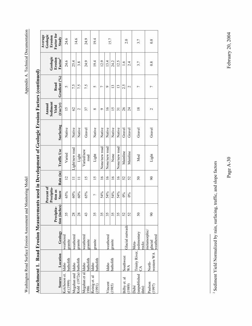
Was
hing
ton
Roa
d Su
rfac
e Er
osio
n A
sses
smen
t and
Mon
itorin
g M
odel
A
ppen
dix
A. T
echn
ical
Doc
umen
tatio
n
Att
achm
ent 1
. R
oad
Ero
sion
Mea
sure
men
ts u
sed
in D
evel
opm
ent o
f Geo
logi
c E
rosi
on F
acto
rs (c
ontin
ued)
Sour
ce
Loc
atio
n G
eolo
gy
Prec
ipita
-tio
n (in
ches
)
Perc
ent o
f Pr
ecip
ita-
tion
as
Snow
R
ain
(in)
Tra
ffic
Use
Su
rfac
ing
Ann
ual
Sedi
men
t Y
ield
(t
/ac/
yr)
Roa
d G
radi
ent (
%)
Geo
logi
c E
rosi
on
Fact
or2
Ave
rage
G
eolo
gic
Ero
sion
Fa
ctor
for
Stud
y K
etch
eson
et.
al (1
999)
Id
aho
bath
olith
w
eath
ered
gr
anite
35
65
%12
Var
ied
Nat
ive
155
24.6
24.6
28
60%
11
Ligh
t/new
road
Nat
ive
627.
525
.4M
egah
an a
nd
Kid
d (1
972a
) Id
aho
bath
olith
w
eath
ered
gr
anite
28
60%
11Li
ght
Nat
ive
27.
53.
814
.6
Meg
ahan
et a
l. 19
86
Idah
o ba
thol
ith
wea
ther
ed
gran
ite
43
65
%15
Var
ied/
new
ro
ad
Gra
vel
377.
524
.924
.9
Rei
nig
et. a
l (1
991)
Id
aho
bath
olith
gr
anite
35?
15Li
ght
Nat
ive
85
19.4
19.4
35
54
%16
N
one/
new
road
Nat
ive
97
12.9
35
54
%16
N
one/
new
road
Nat
ive
169
13.4
35
54
%16
Non
eN
ativ
e15
1324
.2V
ince
nt
(198
5)
Idah
o ba
thol
ith
wea
ther
ed
gran
ite
35
54
%16
N
one/
new
road
Nat
ive
3113
12.5
15.7
52
0%52
M
ainl
ine
Gra
vel
262.
51.
6B
ilby
et. a
l (1
989)
So
uthw
est
WA
G
laci
al o
utw
ash
52
0%
52M
ainl
ine
Gra
vel
242
2.4
2.0
Dub
é (u
npub
lishe
d da
ta)
Trin
ity R
iver
, C
A
Met
a-se
dim
enta
ry
rock
s 50
50
Mod
Gra
vel
187
3.7
3.7
Paul
son
(199
7)
Nor
th-
wes
tern
WA
met
amor
phic
/ gl
acia
l w
eath
ered
90
90
Ligh
tG
rave
l2
70.
80.
8
2 S
edim
ent Y
ield
Nor
mal
ized
by
rain
, sur
faci
ng, t
raff
ic, a
nd sl
ope
fact
ors
Pa
ge A
-30
Febr
uary
20,
200
4

Was
hing
ton
Roa
d Su
rfac
e Er
osio
n A
sses
smen
t and
Mon
itorin
g M
odel
A
ppen
dix
A. T
echn
ical
Doc
umen
tatio
n
Att
achm
ent 1
. R
oad
Ero
sion
Mea
sure
men
ts u
sed
in D
evel
opm
ent o
f Geo
logi
c E
rosi
on F
acto
rs
Sour
ce
Loc
atio
n G
eolo
gy
Prec
ipita
-tio
n (in
ches
)
Perc
ent o
f Pr
ecip
ita-
tion
as
Snow
R
ain
(in)
T
raff
ic U
se
Surf
acin
g
Ann
ual
Sedi
men
t Y
ield
(t
/ac/
yr)
Roa
d G
radi
ent (
%)
Geo
logi
c E
rosi
on
Fact
or 3
Ave
rage
G
eolo
gic
Ero
sion
Fa
ctor
for
Stud
y 37
50%
19
Hea
vyN
ativ
e1
50.
237
50%
19H
eavy
Gra
vel
07
0.2
37
50
%19
Hea
vyG
rave
l2
71.
037
50%
19H
eavy
Nat
ive
36
0.3
37
50
%19
Ligh
tN
ativ
e1
60.
837
50%
19Li
ght
Nat
ive
04
0.3
37
50
%19
Ligh
tN
ativ
e1
0.8
31
50
%16
Nat
ive
05
0.2
50%
16Li
ght
7Li
ght
31
N
ativ
e1
61.
031
50%
16H
eavy
Nat
ive
26
0.4
31
50
%16
Hea
vyN
ativ
e2
40.
631
50%
16H
eavy
Gra
vel
27
0.9
Toth
(200
0)
Cen
tral W
A
sand
ston
e
31
50
%16
Hea
vyN
ativ
e4
70.
5
0.6
3 S
edim
ent Y
ield
Nor
mal
ized
by
rain
, sur
faci
ng, t
raff
ic, a
nd sl
ope
fact
ors
Pa
ge A
-31
Febr
uary
20,
200
4

Was
hing
ton
Roa
d Su
rfac
e Er
osio
n A
sses
smen
t and
Mon
itorin
g M
odel
A
ppen
dix
A. T
echn
ical
Doc
umen
tatio
n
Att
achm
ent 1
. R
oad
Ero
sion
Mea
sure
men
ts u
sed
in D
evel
opm
ent o
f Geo
logi
c E
rosi
on F
acto
rs
Sour
ce
Loc
atio
n G
eolo
gy
Prec
ipita
-tio
n (in
ches
)
Perc
ent o
f Pr
ecip
ita-
tion
as
Snow
R
ain
(in)
Tra
ffic
Use
Su
rfac
ing
Ann
ual
Sedi
men
t Y
ield
(t
/ac/
yr)
Roa
d G
radi
ent (
%)
Geo
logi
c E
rosi
on
Fact
or4
Ave
rage
G
eolo
gic
Ero
sion
Fa
ctor
for
Stud
y 78
5%
74
Li
ght/n
ew ro
adN
ativ
e
52
5 2.
9
94
5%87
mod
erat
e/ne
w
road
N
ativ
e16
05
1.4
78
5%
74
Ligh
t/new
road
Nat
ive
555
3.0
80
5%
80
Li
ght
Nat
ive
185
3.5
78
5%
74
Ligh
t/new
road
Pitru
n50
101.
4
94
5%87
mod
erat
e/ne
w
road
Pi
trun
120
100.
5
78
5%
74
Ligh
t/new
road
Pitru
n11
510
3.2
80
5%
80
Li
ght
Pitru
n25
102.
578
5%74
Li
ght/n
ew ro
adG
rave
l4
51.
1
94
5%87
mod
erat
e/ne
w
road
G
rave
l14
50.
6
78
5%
74
Ligh
t/new
road
Gra
vel
85
2.2
80
5%
80Li
ght
Gra
vel
55
4.9
2.3
78
5%
74
Ligh
t/new
road
Gra
vel
126
2.3
94
5%87
mod
erat
e/ne
w
road
G
rave
l12
06
3.6
78
5%
74
Ligh
t/new
road
Gra
vel
756
14.4
80
5%
80Li
ght
Gra
vel
306
20.5
78
5%
74
Ligh
t/new
road
Pitru
n26
81.
1
94
5%87
mod
erat
e/ne
w
road
Pi
trun
170
81.
2
78
5%
74
Ligh
t/new
road
Pitru
n65
82.
880
5%80
Ligh
tPi
trun
408
6.1
Swift
(198
4)
App
alac
hian
M
ount
ains
w
eath
ered
gn
eiss
/sch
ist
6.5
4 S
edim
ent Y
ield
Nor
mal
ized
by
rain
, sur
faci
ng, t
raff
ic, a
nd sl
ope
fact
ors
Pa
ge A
-32
Febr
uary
20,
200
4

Was
hing
ton
Roa
d Su
rfac
e Er
osio
n A
sses
smen
t and
Mon
itorin
g M
odel
A
ppen
dix
A. T
echn
ical
Doc
umen
tatio
n
Att
achm
ent 1
. R
oad
Ero
sion
Mea
sure
men
ts u
sed
in D
evel
opm
ent o
f Geo
logi
c E
rosi
on F
acto
rs
Sour
ce
Loc
atio
n G
eolo
gy
Prec
ipita
-tio
n (in
ches
)
Perc
ent o
f Pr
ecip
ita-
tion
as
Snow
R
ain
(in)
Tra
ffic
Use
Su
rfac
ing
Ann
ual
Sedi
men
t Y
ield
(t
/ac/
yr)
Roa
d G
radi
ent (
%)
Geo
logi
c E
rosi
on
Fact
or5
Ave
rage
G
eolo
gic
Ero
sion
Fa
ctor
for
Stud
y 13
0%
13
Li
ght
Pitru
n12
12
11.6
47
48
%25
mod
Pitru
n34
312
27.6
29
0%
29H
eavy
Pitru
n30
212
9.5
71
0%
71N
one
Pitru
n37
1214
.913
0%13
Ligh
tG
rave
l3
127.
947
48%
25m
odG
rave
l20
124.
029
0%29
Hea
vyG
rave
l64
125.
1
Foltz
(199
6)
199
2-95
se
dim
enta
ry
rock
s
71
0%
71N
one
Gra
vel
812
8.1
11.1
79
0%
79Li
ght
Gra
vel
57.
52.
3Lu
ce a
nd
Bla
ck (1
999a
) Wes
tern
OR
se
dim
enta
ry
rock
s 79
0%79
Ligh
tG
rave
l2
7.5
1.1
1.7
52
0%
52
Non
e/ne
w ro
adG
rave
l4
74.
760
0%
60
Hea
vyG
rave
l7
70.
555
0%55
Hea
vyG
rave
l6
70.
555
0%55
Hea
vyG
rave
l6
70.
652
0%
52
Ligh
t/new
road
Nat
ive
389
1.1
60
0%60
H
eavy
Nat
ive
539
0.5
55
0%
55H
eavy
Nat
ive
519
0.5
55
0%
55H
eavy
Nat
ive
489
0.5
52
0%52
Li
ght/n
ew ro
adPi
trun
311
0.1
60
0%60
H
eavy
Pitru
n10
110.
155
0%55
Hea
vyPi
trun
711
0.1
55
0%
55H
eavy
Pitru
n7
110.
152
0%52
Hea
vyG
rave
l4
31.
960
0%60
Hea
vyG
rave
l8
33.
255
0%55
Hea
vyG
rave
l9
34.
1
Koc
hend
erfe
r an
d H
elve
y (1
984)
App
alac
hian
M
ount
ains
se
dim
enta
ry
rock
s
55
0%
55H
eavy
Gra
vel
43
1.8
1.3
5 S
edim
ent Y
ield
Nor
mal
ized
by
rain
, sur
faci
ng, t
raff
ic, a
nd sl
ope
fact
ors
Pa
ge A
-33
Febr
uary
20,
200
4

Was
hing
ton
Roa
d Su
rfac
e Er
osio
n A
sses
smen
t and
Mon
itorin
g M
odel
A
ppen
dix
A. T
echn
ical
Doc
umen
tatio
n
Att
achm
ent 1
. R
oad
Ero
sion
Mea
sure
men
ts u
sed
in D
evel
opm
ent o
f Geo
logi
c E
rosi
on F
acto
rs
Sour
ce
Loc
atio
n G
eolo
gy
Prec
ipita
-tio
n (in
ches
)
Perc
ent o
f Pr
ecip
ita-
tion
as
Snow
R
ain
(in)
Tra
ffic
Use
Su
rfac
ing
Ann
ual
Sedi
men
t Y
ield
(t
/ac/
yr)
Roa
d G
radi
ent (
%)
Geo
logi
c E
rosi
on
Fact
or6
Ave
rage
G
eolo
gic
Ero
sion
Fa
ctor
for
Stud
y 19
6
0%
196
Mod
Gra
vel
276.
4 0.
8W
ald
(197
5)
Oly
mpi
c Pe
nins
ula,
W
A
sedi
men
tary
ro
cks
196
0%
196
Ligh
tG
rave
l2
31.
21.
0
140
0%
140
Mai
nlin
eG
rave
l38
25.
51.
114
0
0%14
0 Te
mp
non-
use
Gra
vel
515.
50.
914
0
0%14
0
Mod
Gra
vel
325.
52.
214
0
0%14
0Li
ght
Nat
ive
35.
50.
215
3
0%15
3M
ainl
ine
Gra
vel
500
100.
415
3
0%15
3 Te
mp
non-
use
Gra
vel
6510
0.3
153
0%
153
M
odG
rave
l40
100.
715
3
0%15
3Li
ght
Nat
ive
410
0.1
Rei
d (1
981)
O
lym
pic
Peni
nsul
a,
WA
sedi
men
tary
ro
cks
153
0%
153
Non
eN
ativ
e1
100.
0
0.7
6 S
edim
ent Y
ield
Nor
mal
ized
by
rain
, sur
faci
ng, t
raff
ic, a
nd sl
ope
fact
ors
Pa
ge A
-34
Febr
uary
20,
200
4

Appendix B. Data Sheets and Field Forms


Su
rfac
e Er
osio
n R
oad
Surv
ey F
ield
/Dat
a En
try
Form
Mgm
t. Bl
ock
Surv
ey D
ate
Sur
veyo
rR
oad
Nam
eW
AUPr
oj. A
rea
T/R
/Sec
T
R
SW
eath
erTr
ead
Ifo
rmat
ion
Segm
ent
Num
ber
(and
gr
oup
if us
ed)
Seg
men
t Le
ngth
(ft)
Year
R
oad
Built
Eros
ion
Rat
ing
(bas
e on
ge
olog
y)L
- low
M -
mod
.H
- hi
gh
Roa
d S
lope
C
lass
<5%
5-10
%>1
0%
Roa
d C
onfig
. I-i
nslo
ped
O-o
utsl
oped
C
-cro
wne
d
Surfa
cing
A-a
spha
ltG
-gra
vel
N-n
ativ
eP
-pitr
unr-w
/ruts
s-w
/gra
ss
Aver
age
Trea
d W
idth
(ft)
Traf
fic U
se
H-h
eavy
MH
-mod
he
avy
M-m
odL-
light
O-o
ccas
.N
-non
e
Cov
er
Den
sity
90
-100
%70
-90%
50-7
0%30
-50%
10-3
0%0-
10%
Aver
age
Hei
ght
(p
ick
clos
est)
25 ft
10 ft
5 ft
2.5
ftno
cut
slop
eW
idth
(ft)
Del
iver
y 0-
none
1-di
rect
to
stre
am2-
w/in
100
ft3-
w/in
200
ft
4-di
rect
via
gu
lly
Con
ditio
nR
-rock
/veg
S-s
tabl
eE
-ero
ding
1 2 3 4 5 6 7 8 9 10
Pro
blem
Are
as/C
omm
ents
Cla
ssM
-mai
nlin
eP-
prim
ary
S-s
econ
dary
Sp-
spur
Pos
ition
R-ri
dget
opM
-mid
slop
eS
-stre
am a
dj.
F-fla
t val
ley
botto
m
1 2 3 4 5 6 7 8 9 10
Cut
slop
e
BMP/
date
Ditc
h
BM
P/d
ate
BMP/
date
BM
P/d
ate
n

Surface Erosion Road Survey Field/Data Entry Form Instructions Attribute Possible
Values How to Measure or Determine
Segment Number and Group ID if used
Unique number; decimals OK
Segment number should be unique, at least within each Project Area. Group ID number can be used to group road segments that are connected but have different attributes (e.g., surfacing). Segment number should be noted on the field map for location reference.
Segment Length Length (feet) Measure length of segment using a tape or measuring wheel. Year Road Built Year Contact landowner. If unknown or old road, estimate to nearest decade. Erosion Rating H, M, L Look at geologic map and determine rating based on Appendix A Table A-1 (pre-field)
Road Slope
Road Slope Class <5% 5-10% >10%
Measure and record average gradient of tread with clinometer or estimate within slope class: <5% - flat or gently sloping road 5-10% - moderately sloped road segment >10% - steep road Average the gradient over entire segment. If the segment is a V-shaped stream crossing, estimate gradient on each side of crossing and average.
Road Configuration
I-insloped (or outsloped w/wheel tracks)
O-outsloped C-crowned
Look at configuration of road prism (see Figure 3 for examples). Evaluate the drainage path of water on the tread – does the entire tread drain to the ditch (insloped); or to the fillslope (outsloped); or is road crowned? In most cases, the road configuration will vary along the segment in subtle ways. Record average configuration. If the road is outsloped/crowned but has wheel tracks (less than 2 inches deep) or ruts (over 2 inches deep) that channel water along the tread and deliver it to the ditch or stream crossing, record it as Insloped. If the road has ditches on each side that deliver, record it as Insloped.
Surfacing
A-asphalt G-gravel N-native P-pitrun r-w/ruts s-w/grass
Determine surfacing on road tread. Use the following guidelines: Gravel - a good gravel surface; little dust or fines on surface Native – dirt surface Pitrun – poor quality gravel surface; lots of fines or dust r or s – used in conjunction with surfacing to indicate ruts (over 2 inches deep) or grassed surface. For example: Gr; Ns.
Average Tread Width Width in feet Measure the full width of tread surface that could be driven on (see Figure B-1) at 3-4
locations to nearest foot. Record average value (nearest foot).
Roa
d Tr
ead
Traffic Use
H-heavy MH-mod heavy M-mod L-light O-occasional N-none
Contact landowner to determine long-term average use of roads (average number of trips by truck/car per day). Use the following guidelines: H: >5 log trucks/day, plus heavy pickups or car traffic MH: 4-5 log trucks/day, >5 pickups or car traffic M: 3-4 log trucks/day, 5-10 pickups or cars/day L: 1-2 log truck/day, 1-5 pickups or cars/day O: <1 log truck/day, <1 pickup or car/day N: no use (abandoned, inactive, or blocked to traffic)
Cover Density
90-100% 70-90% 50-70% 30-50% 10-30% 0-10%
Determine the average percent of the cutslope area that is covered with vegetation, rock, leaf litter, or other non-erodible material.
Cut
slop
e
Average Height
25 ft 10 ft 5 ft 2.5 ft no cutslope
Average height of cutslope (slope length). Cutslope height often varies considerably in field (especially at stream crossings where it may range from 0 at stream to 10’s of feet high). See Figure 2
Width Width in feet Measure width of ditch at 3-4 locations. Record average value (nearest foot)
Delivery
0-none 1-direct 2-w/in 100 ft 3-w/in 200 ft 4-direct via gully
Determine delivery of ditch, drainage outfall, or road segment if outsloped. 1 (direct delivery) – drains directly into stream channel 2 (w/in 100 ft) – drains to forest floor; stream is 1-100 feet away 3 (w/in 200 ft) – drains to forest floor; stream is 101-200 feet away 4 – is connected directly to stream via a gully D
itch
Condition R-rock/veg S-stable E-eroding
R – ditch has been rocked or is vegetated S – ditch appears stable (not eroding) E – ditch is eroding/incising.
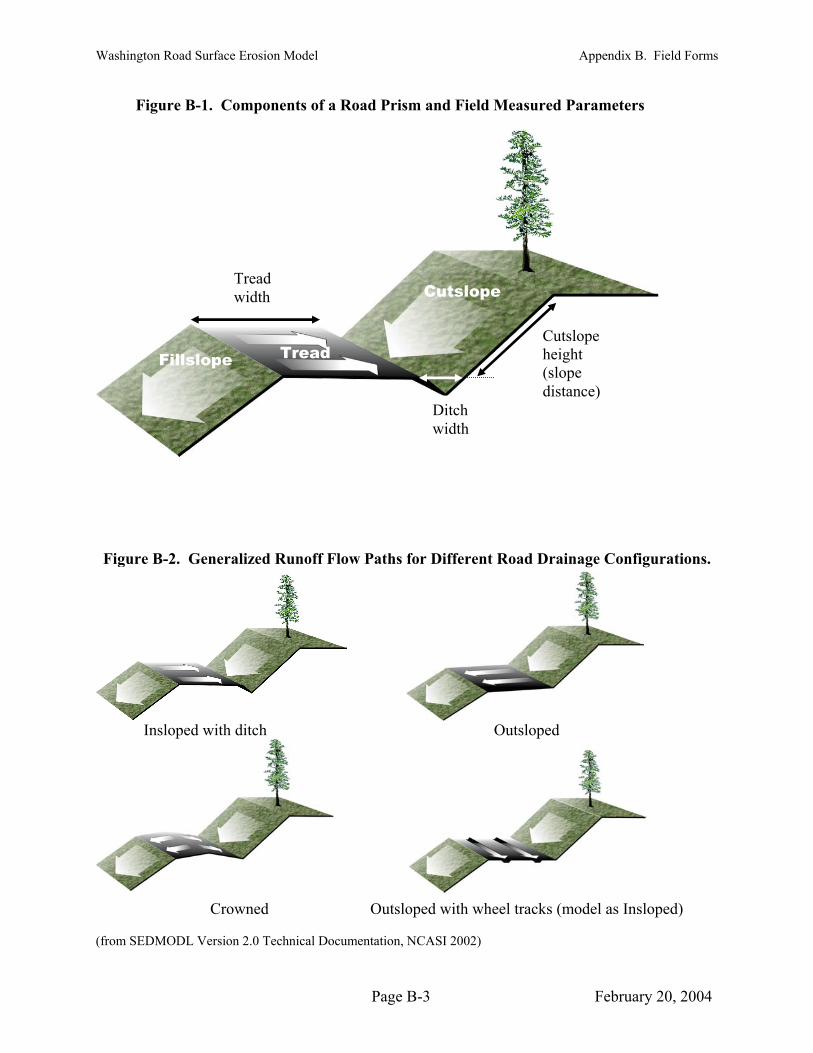
Washington Road Surface Erosion Model Appendix B. Field Forms
Figure B-1. Components of a Road Prism and Field Measured Parameters
Tread width Cutslope
Cutslope height d Fillslope
Figure B-2. Generalized
Insloped with ditch
Crowned (from SEDMODL V
ersion 2.0 Te
Trea
Ditch width
(slope distance)
ths for Different Road Drainage Configurations. Runoff Flow Pa
Outsloped
Outsloped with wheel tracks (model as Insloped)
chnical Documentation, NCASI 2002)
Page B-3 February 20, 2004
Washington Road Surface Erosion Model Appendix B. Field Forms
Typical Road Surfacing Types r staff) (Photos courtesy of Weyerhaeuse
Gravel Pitrun/worn gravel
Grass/Gravel with Wheel Tracks Grassed
Wheel Tracks Rutted
Page B-4 February 20, 2004

Washington Road Surface Erosion Model Appendix B. Field Forms
Cutslope Cover Percentage Examples
90% Cover Density (10% Bare Soil) 70% Cover Density 50% Cover Density 30% Cover Density 10% Cover Density
(white patches represent bare soil)
Page B-5 February 20, 2004

Washington Road Surface Erosion Model Appendix B. Field Forms
BMP Reference List
1. Gravel road 2. Asphalt road 3. Vegetate road 4. Dust/oil surface 5. Chipseal road 6. Apply dust abatement7. Geotextile use on wetland roads to reduce ruts 8. Sand/cinder application for snow/ice 9. Rock or armor fords 10. Low pressure truck tires on native road 11. Low pressure truck tires on pitrun roads 12. Low pressure truck tires on gravel roads 13. Seal bridge deck 14. Road grading 20. Daylight roads (rem21. Close road to traffic (gate o22. Restrict access (to light use) 23. Haul only during summer (June-October) 24. Haul only on frozen roads (m25. Cease hauling during spring breakup (m26. Cease hauling when30. Apply hydromulch to31. Apply straw to cutslope 32. Apply straw + net to cutslope 33. Apply erosion mat 34. Bench cutslopes 35. Stabilize (buttress)40. Outslope roads 41. Crown roads 50. Install driveable dip 51. Install cross drain cu52. Install waterbars (cons53. Belt diverters/surface water deflectors 54. Double ditch 55. Bypass ditch 56. Place berm57. Rem58. Rem60. Protect drainage stru61. Install settling basins62. Install silt fences/hay63. Vegetate/rock ditch 64. Filter windrow at cu
on road surface
ove shade trees – drier roads) r tank trap)
id-Novemb
road runoff reaches streams on mainline roads
cutslope
idered temporary feature)
on outside shoulder of road ove outside berm on outsloped road ove outside berm on crowned road
ales at outf
lvert outfall
70. Decommission road
er – mid-Feb) id-Feb – mid-April)
cutslope
lvert
cture outfall with rip rap
all or in ditchline b
65. Curbs/splash guards on bridges
Page B-6 February 20, 2004

Washington Road Surface Erosion Model Appendix B. Field Forms
Common Road Problems (can be included in notes field in Access Application)
blems: re – shallow re – deep-seated (slump or earthflow)
ravel rings in cutslope
ilure (fill cracking, sagging of road fill or tread)
ms
around culvert) past cross drain further down the road or ditch – usually causes
ead)
osed road (similar effects as c above) ow cross drain culvert or cross ditch
ulvert, or puncheon wn ditchline before entering culvert
routed down ditchline more than 50 feet before entering culvert
arriers (on fish-bearing stream crossings) drop at outlet (shotgun)
1 crossing
w/o stream substrate
rphan road
deck
1. Cutslope proa. Mass failub. Mass failuc. Chronic dry d. Seeps or sp
2. Fillslope problems
a. Mass failure b. Incipient mass fac. Steep fillslopes d. Perched landings e. Unvegetated fillslope
3. Drainage proble
a. Cross drain culvert washout b. Incipient cross drain washout (pipingc. Plugged cross drain (flow
excessive erosion of ditch or road trd. Excessive rutting (ruts > 3 inches deep) e. Fill washout at channel crossings f. Failure on hillslope below road caused by road runoff g. Failure of cross ditches on clh. Gully on hillslope beli. Old or rusted culvert, box cj. Stream routed dok. Spring or seepl. Ditchline eroded/gullied
4. Fish Passage B
a. Culverts have b. Multiple culverts atc. Small diameter culvert d. Steep gradient in culvert e. Culvert
5. Other
a. Stream crossing with deep fill on ob. Undersized culvert c. Ford d. Holes in bridgee. Eroding bridge abutments
Page B-7 February 20, 2004

Washington Road Surface Erosion Model Appendix B. Field Forms
Page B-8 February 20, 2004

Appendix C. Best Management Practices

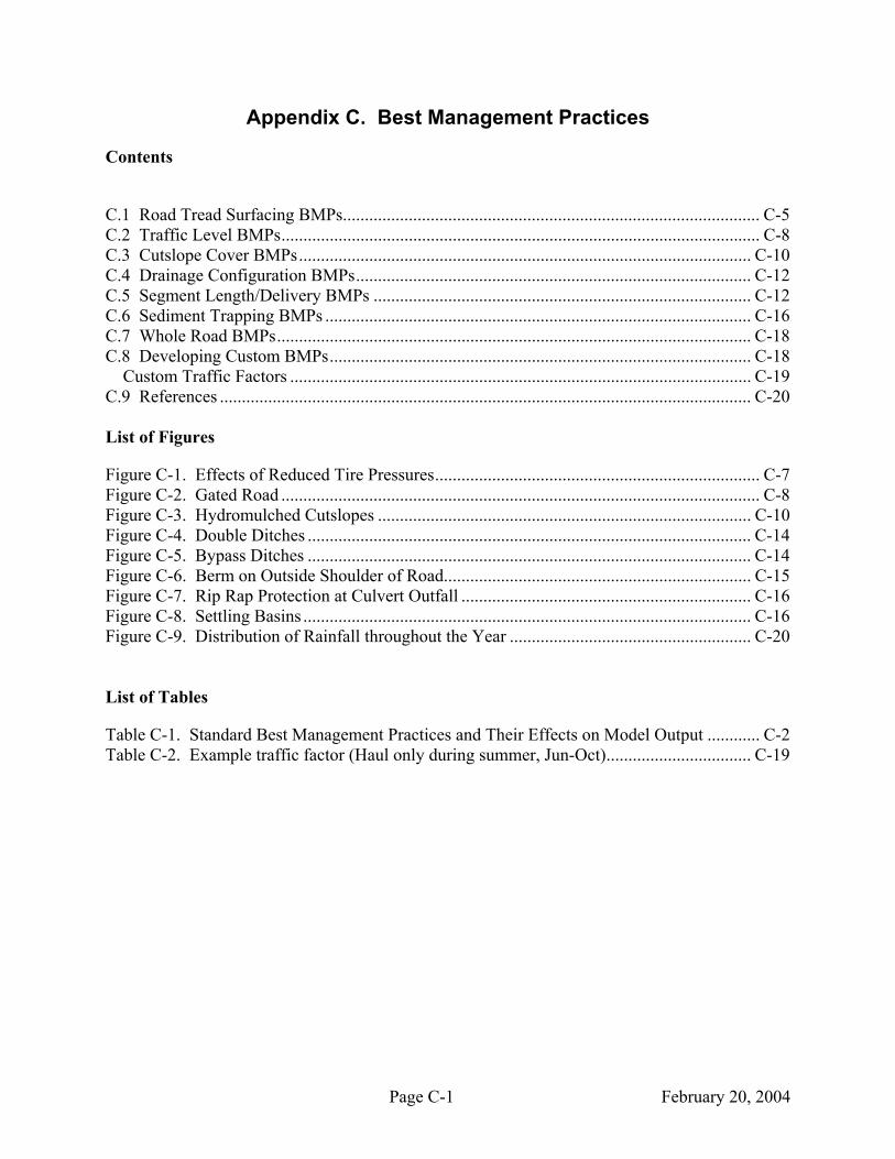
Appendix C. Best Management Practices
Contents
C.1 Road Tread Surfacing BMPs............................................................................................... C-5 C.2 Traffic Level BMPs............................................................................................................. C-8 C.3 Cutslope Cover BMPs....................................................................................................... C-10 C.4 Drainage Configuration BMPs.......................................................................................... C-12 C.5 Segment Length/Delivery BMPs ...................................................................................... C-12 C.6 Sediment Trapping BMPs ................................................................................................. C-16 C.7 Whole Road BMPs............................................................................................................ C-18 C.8 Developing Custom BMPs................................................................................................ C-18
Custom Traffic Factors ......................................................................................................... C-19 C.9 References ......................................................................................................................... C-20 List of Figures
Figure C-1. Effects of Reduced Tire Pressures.......................................................................... C-7 Figure C-2. Gated Road ............................................................................................................. C-8 Figure C-3. Hydromulched Cutslopes ..................................................................................... C-10 Figure C-4. Double Ditches ..................................................................................................... C-14 Figure C-5. Bypass Ditches ..................................................................................................... C-14 Figure C-6. Berm on Outside Shoulder of Road...................................................................... C-15 Figure C-7. Rip Rap Protection at Culvert Outfall .................................................................. C-16 Figure C-8. Settling Basins ...................................................................................................... C-16 Figure C-9. Distribution of Rainfall throughout the Year ....................................................... C-20 List of Tables
Table C-1. Standard Best Management Practices and Their Effects on Model Output ............ C-2 Table C-2. Example traffic factor (Haul only during summer, Jun-Oct)................................. C-19
Page C-1 February 20, 2004

Washington Road Surface Erosion Model Appendix C. Best Management Practices
Page C-2 February 20, 2004
application for snow/ice
Appendix C. Best Management Practices
Landowners apply a number of different road maintenance practices or improvements to reduce either sediment production (erosion) or delivery to streams. Collectively, these are often referred to as Best Management Practices (BMPs). BMPs may affect only one part of the road prism, for example surfacing of the road tread, or they may affect more than one factor. Installing a cross drain culvert in a road section that drains to a stream crossing reduces the length of road delivering sediment to the stream, and changes the delivery of sediment upslope of the cross drain to indirect delivery.
A list of the most commonly applied BMPs affecting road surface erosion/delivery is shown in Table C-1 and further described below. Research on road erosion has yielded information on the numerical effects of some BMPs on erosion/delivery. If the effects of BMPs have been reported, the change in model factor(s), or change in the way the model computes erosion or deliver are listed in Table C-1. For many BMPs, there is not currently sufficient supporting research to establish specific numerical effects. These BMPs are listed with an “X” in Table C-1. The user can specify that these BMPs have been applied to road segments, but there will be no change in computed erosion/delivery at this time. Future updates of model values may include values for these BMPs as road research becomes available.
In addition to the standard BMPs listed below, the user can also create Custom BMPs if they apply BMPs on their roads that are not listed in Table C-1. The model allows the user to enter numerical effects of these custom BMPs, and will apply the specified factors in erosion computations. Users doing this should be prepared to provide justification for the values selected based on research reports, data from local observations, etc. Procedures for entering custom BMPs are included following the description of standard BMPs.
Table C-1. Standard Best Management Practices and Their Effects on Model Output Erosion Rate Delivery
BMP
Seg-ment
Length
Surfac-ing Width Traffic
Use
Cut- slope Cover
Cut-slope
Height
Road Config-uration.
Delivery (type or %)
1. Gravel road Gravel (0.2)
2. Asphalt road Aspha
lt (0.03)
3. Vegetate road
Grassed
native (0.5)
4. Dust/oil surface 0.15 5. Chipseal road X 6. Apply dust abatement on road surface X
7. Geotextile use on wetland roads to reduce ruts
X
8. Sand/cinder X
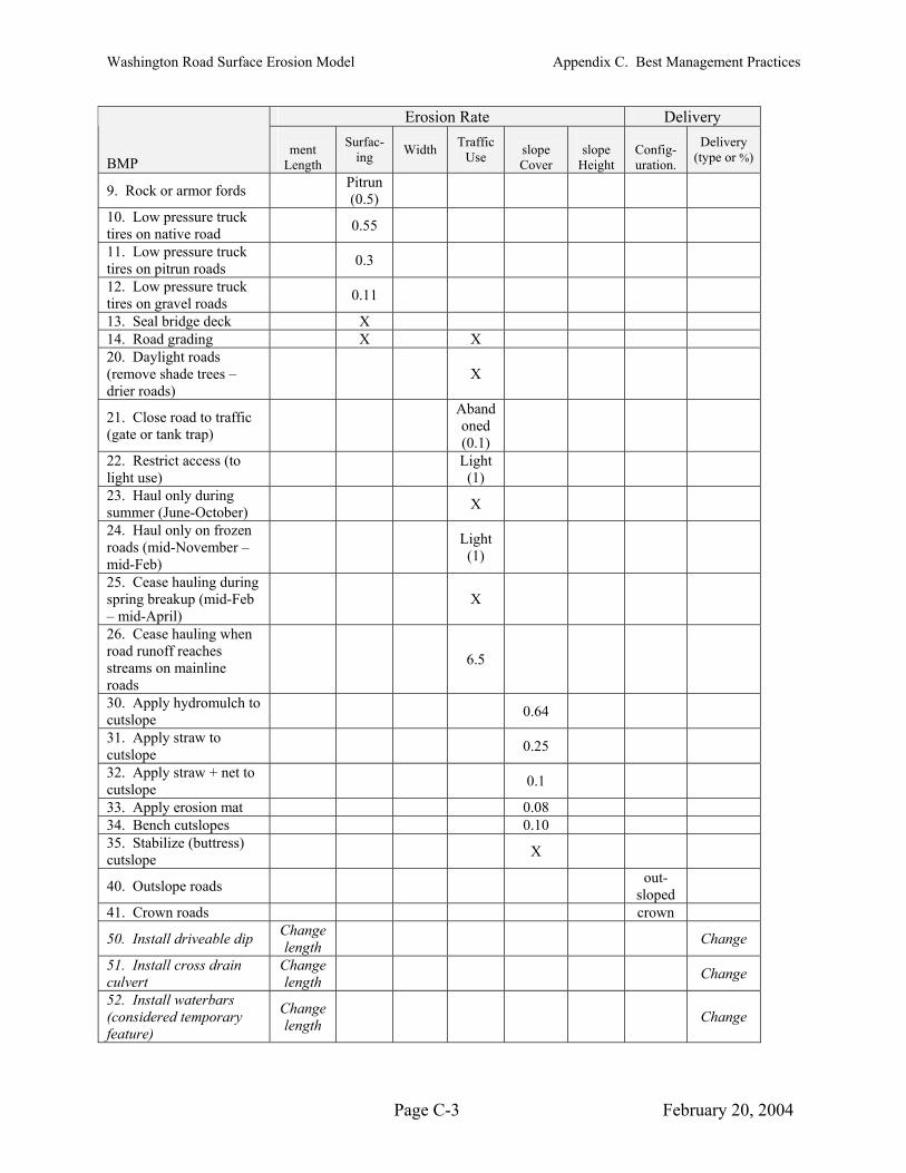
Washington Road Surface Erosion Model Appendix C. Best Management Practices
Erosion Rate DeliverySeg- Cut- Cut- Road
ment Length
Surfac-ing Width Traffic
Use slope Cover
slope Height BMP
Config-uration.
Delivery (type or %)
9. Rock or armor fords Pitrun (0.5)
10. Low pressure truck tires on native road 0.55
11. Low pressure truck 0.3 tires on pitrun roads 12. Low pressure truck tires on gravel roads 0.11
13. Seal bridge deck X 14. Road grading X X 20. Daylight roads
move shade trees – X (redrier roads)
Aband21. Close road to traffic oned (0.1)
(gate or tank trap)
22. Restrict access (to Light light use) (1)
23. Haul only during X summer (June-October) 24. Haul only on frozen roads (mid-November – Light mid-Feb) (1)
25. Cease hauling during spring breakup (mid-Feb X – mid-April) 26. Cease hauling when road runoff reaches streams on mainline
ads
6.5
ro30. Apply hydromulch to cutslope 0.64
31. Apply straw to 0.25 cutslope 2. Apply straw + net to 3
cutslope 0.1
33. Apply erosion mat 0.08 34. Bench cutslopes 0.10 35. Stabilize (buttress) cutslope X
40. Outslope roads out-sloped
41. Crown roads crown
50. Install driveable dip Change length Change
51. Install cross drain culvert
Change length Change
52. Install waterbars (considered temporary feature)
Change length Change
Page C-3 February 20, 2004

Washington Road Surface Erosion Model Appendix C. Best Management Practices
Erosion Rate DeliverySeg- Cut- Cut- Road
BMP ment
Length ing Width Use slope Cover
slope Height
Config-uration. (type or %)
53. Belt diverters/ surface water deflectors
Change length Change
54. Double ditch Change length X
55. Bypass ditch Change length X
56. Place berm on Cha
Surfac- Traffic Delivery
outside shoulder of road nge
length In-sloped
57. Remove outside berm on outsloped road
Change length out-
sloped
58. Remove outside berm on crowned road
Change length crown
60. Protect drainage structure outfall with rip rap
50%
61. Install settling basins 15% 62. Install silt fences/hay bales at outfall or in ditchline
75%
63. Vegetate/rock ditch X 64. Filter windrow at culvert outfall X
65. Curbs/splash guards on bridges X
70. Decommission road X Grass (0.5)
Abandoned (0.1)
n/a 0 Out-sloped
No(1) (2) Numerical/text effects indicate new factor tha in model. (3) Italicized BMPs (50-58) relate to installation of measu duc lengt oad n s.
BMPs require the user t the r d e ite-s da rai u n and e from stream for the n e
There are a number of excellent c tions of the effectiveness of forestry and road BMPs. (1996) comp ed all r arch lated t BMPs the st e of Id o, inclu ing
general erosion research and timber harvesting BMPs as well as road construction and maintenance BMPs. NCASI (2000) has a draft technical bulletin on the effectiveness of BMPs
ir web site esearch/watershed/control.pdf
tes: X indicates insufficient research to support numerical effect at present time.
t will be appliedres to re
nter se the pecific
h of rta on d
deliverinage str
g to streamcture locatioThese
distanco splitew segm
oad segment annts.
aompileseSeyedbagheri il re o in at ah d
available on the (http://www.ncasi.org/forestry/r
wetlands and fish w s othpublications on vetread, or sediment trap /r on
The following secsupporting the numer f ted e P tAppendix A (
) summarizing research on BMPs for roads, timber harvest/site preparation, riparian areas,
habitat as ell a er areas. In addition there are many individual the effectiveness of getation and erosion control on cut and fill slopes, road
ping unoff c trol.
tions describe each standard BMP listed in Table C-1 and the research ical ef ects lis . Sev ral BM s refer o sections, figures, and tables in
e.g., Section A.2 and Table A-3).
Page C-4 February 20, 2004

Washington Road Surface Erosion Model Appendix C. Best Management Practices
C.1 Road Tread Surfacing BMPs
1. Gravel road
Description: Applying goo qual vel a native surface road reduces surface ero ion by material from raindrop impact and overland flow by making the surface less
aking dow into ble p rticles, and by reducing rutting. Most studies found ver 4 ches) lean avel was most effective at reducing surface erosion.
han 4 inches) layers of gravel, or soft gravel was not as effective at reducing
d ity gra to sprotecting the native susceptible to bre n erodi athat a thicker layer (oPitrun, thin (less t
in of c gr
surface erosion.
Effectiveness: Gravel redu es surf erosi n of the tread by approximately 80 percent (see ferences in Section A.2 and Table A-2). No references were found numerically
s to gra el dura
c ace odiscussion and rerelating erosion rate v bility.
2. Asphalt road
Description: Applytread to m
ing an asphalt surface to a roa ctively reduces surface erosion from the inimal amounts. However, erosion in the ditchline and at culvert outfalls can still
ease due to increased runoff from the paved surface unless ditch protection is
d effe
occur and may incrprovided.
Effectiveness: Asphadiscussio
lt red es surf e eros n of tread appro imately 97-99 percent (see n and references in Section A.2 and Table A-2). Surface erosion still can occur in the
utfa unless they are also treated (se itch treatments in a sepa ate
d
iption:
uc ac io the by x
ditch or at the culvert osection).
ll e d r
3. Vegetate roa
Descrvegetate naturally; road s .
Effectiveness: Vegetated r d surfa es yield approximately half thatferences in Section A.2 and Table A-2).
oa c of native surfaced roads (see discussion and re
4. Dust/oil surface
Description: Applyiparticles tog
ng a du t oil tre tment temporarily seals the road surface and bind surface ether, making them resistant to erosion and reducing dust.
s a s
Effectiveness: percent (see dis
Dust oil trea ment re uces surface erosion of the tread by approximately 85 cussion renc s in Se ion A and Ta le A-2
t deand refe ct .2 b ).
5. Chipseal road
Description: Applyerosion and is very sunder h
ing al surface, essentially a thin layer of asphalt, seals the road from imilar to asphalt. However, the surface is subject to wear, and breaks down
eavy traffic more readily than a thicker asphalt surface, producing potholes and some resulting surface erosion.
a chip se
Grass or vegetation growing on the road tread reduces erosion. Unused roads often s can also be eeded
Page C-5 February 20, 2004
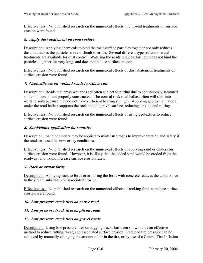
Washington Road Surface Erosion Model Appendix C. Best Management Practices
Effectiveness: No published research on the numerical effects of chipseal trea surface erosion were found.
batem oad surface
Description:
tments on
6. Apply dust a ent on r
chemicacles modust, but makes
treatments are a for dust tr a
Effectiveness: No pubsurface erosion w
li earch on the numerical effects of dust aba treatments on ere fou
use on w road to red ce ru
shed resnd.
te ntme
7. Geotextile etland s u ts
Description: Roads tsoil
hat cro s wetla ds are ften su ject to rutting due to continuously saturated conditions if not properly constructed. The normal rock road ballast often will sink into
they do not have sufficient bearing strength. Applying geotex aterial last supports the r gravel surface, reducing sinking and rutting.
s n o b
wetland soils because under the road bal
tile mock and the
Effectiveness: No publishe researc on the numerical effects of using geotextiles to reduce e found
licatio for sn w/ice
d hsurface erosion wer .
8. Sand/cinder app n o
Description: Sand or cind may be applied to winter use roads to improve traction and safety if the roads are used in snow or icy c ions.
ersondit
Applying ls to bind the road surface particles together not only reduces the parti re difficult to erode. Several different types of commercial vailable con ol. W tering the roads reduces dust, but does not bind the
particles together for very long, and does not reduce surface erosion.
Effectiveness: No published research on the numerical effects of appsurface erosion were found. However, it is likely that the added roadway, and would increase
lying sand or cinders on sand would be eroded from the
surface erosion rates.
9. Rock or armor fords
Description: Applying rock to fords or armoring the fords with concrete reduces the disturbancto the stream substrate and associated erosion.
Effectiveness:
e
No published research on the numerical effects of rocking fords to reduce surfaceerosion were found.
10. Low pressure truck tires on native road
11. Low pressure truck tires on pitrun ro
ads
12. Low pressure truck tires on gravel roads
Description: Using low pressure tires on logging trucks has been shown to be an effective method to reduce rutting, wear, and associated surface erosion. Reduced tire pressure can be achieved by manually changing the amount of air in the tire, or by use of a Central Tire Inflation
Page C-6 February 20, 2004
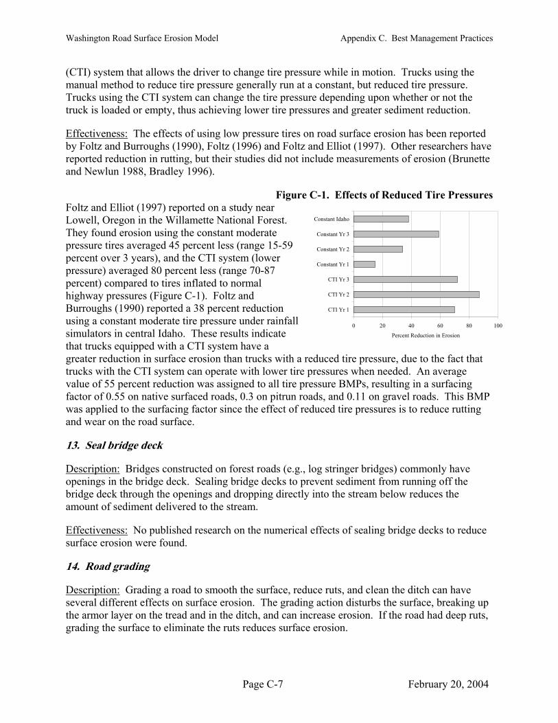
Washington Road Surface Erosion Model Appendix C. Best Management Practices
0 20 40 60 80 100
Constant Yr 1
Constant Yr 2
Constant Yr 3
ange tire pressure while in motion. Trucks using the manual method to reduce tire pressure generally run at a constant, but reduced tire pressure. T CTI system can change the tire pressure depending upon whether or not the truck is loaded or empty, thus achieving lower tire pressures and greater sediment reduction.
(CTI) system that allows the driver to ch
rucks using the
Effectiveness: The effects of using low pressure tires on road surface erosion has been reported by Foltz and Burroughs (1990), Foltz (1996) and Foltz and Elliot (1997). Other researchers have reported reduction in rutting, but their studies did not include measurements of erosion (Brunette and Newlun 1988, Bradley 1996).
Constant Idaho
Foltz and Elliot (1997) reported on a study near Lowell, Oregon in the Willamette National Forest. They found erosion using the constant mode
CTI Yr 1
CTI Yr 2
CTI Yr 3pressure) averaged 80 percent less (range 70-87 percent) compared to tires inflated to normal highway pressures (Figure C-1). Foltz and Burroughs (1990) reported a 38 percent reduction using a cons
Percent Reduction in Erosionsimulators in central Idaho. These results indicate that trucks equipped with a CTI system have a greater reduction in surface erosion than trucks with a reduced tire pressure, due to the fact that trucks with the CTI system can operate with lower tire pressures when needed. An averagevalue of 55
Figure C-1. Effects of Reduced Tire Pressures
rate pressure tires averaged 45 percent less (range 15-59 p rs), and the CTI system (lower
tant moderate tire pressure under rainfall
percent reduction was assigned to all tire pressure BMPs, resulting in a surfacing
factor of 0.55 on native surfaced roads, 0.3 on pitrun roads, and 0.11 on gravel roads. This BMP was applied to the surfacing factor since the effect of reduced tire pressures is to reduce rutting
13. Seal bridge deck
ercent over 3 yea
and wear on the road surface.
Description: Bridges constructed on forest roads (e.g., log stringer bridges) commonly have openings in the bridge deck. Sealing bridge decks to prevent sediment from running off the bridge deck through the openings and dropping directly into the stream below reduces the amount of sediment delivered to the stream.
Effectiveness: No published research on the numerical effects of sealing bridge decks to reduce surface erosion were found.
D
14. Road grading
escription: Grading a road to smooth the surface, reduce ruts, and clean the ditch can have several different effects on surface erosion. The grading action disturbs the surface, breaking up the armor layer on the tread and in the ditch, and can increase erosion. If the road had deep ruts, grading the surface to eliminate the ruts reduces surface erosion.
Page C-7 February 20, 2004
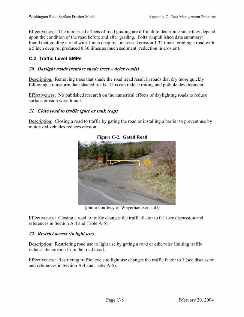
Washington Road Surface Erosion Model Appendix C. Best Management Practices
Effectiveness: The numerical effects of road grading are difficult to determine since they dependupon the condition of
the road before and after grading. Foltz (unpublished data summary)
found that grading a road with 1 inch deep ruts increased erosion 1.32 times; grading a road with a h sediment (reduction in erosion).
Description:
5 inch deep rut produced 0.36 times as muc
C.2 Traffic Level BMPs
20. Daylight roads (remove shade trees – drier roads)
Removing trees that shade the road tread result in roads that dry more quickly
Effectiveness:
following a rainstorm than shaded roads. This can reduce rutting and pothole development.
No published research on the numerical effects of daylighting roads to reduce s nurface erosion were fou d.
21. Close road to traffic (gate or tank trap)
Description: Closing a road to traffic by gating the road or installing a barrier to prevent use by motorized vehicles reduces erosion.
Figure C-2. Gated Road
(photo courtesy of Weyerhaeuser staff)
Effectiveness: Closing a road to traffic changes the traffic factor to 0.1 (see discussion and references in Section A.4 and Table A-5).
to light use)
D
22. Restrict access (
escription: Restricting road use to light use by gating a road or otherwise limiting traffic reduces the erosion from the road tread.
Effectiveness: Restricting traffic levels to light use changes the traffic factor to 1 (see discussion and references in Section A.4 and Table A-5).
Page C-8 February 20, 2004
Washington Road Surface Erosion Model Appendix C. Best Management Practices
23. Haul only during summer (June-October)
Description: In some areas of the state, the majority of the precipitation occurs during the months of November through May. Land managers may choose to limit hauling during the winter months in some parts of their road system to reduce erosion and road damage during the wet winter months.
Effectiveness: The effectiveness of this BMP varies depending upon the traffic levels during the remainder of the year. To apply numerical values for specific road sections, create a Custom BMP (described in following section) and select the appropriate traffic levels by month.
r – mi24. Haul only on frozen roads (mid-Novembe
Description: In some parts of the state, timber hasales are planned to allow exclusive hauling during thsystem, the winter haul BMP may be applied.
Effectiveness: Hauling on frozen, snow coverthe roadway is protected by snow, and thereis used to represent light use throughout the year evsnow conditions.
25. Cease hauling during spring breakup (mid-
Description: In areas of the state that receive a winter snowpack, spring break up generally occurs between mid-February and mid-April. During this time, thawing road surfaces and snowmelt result in saturated roadways that form ruts very easily. Many land managers choosestop or limit hauling during this time to prevent damage to the roads and aquatic resources.
Effectiveness:
to
The effectivenes
d-Feb)
ling on frozen roads is possible. If timber winter on some portions of the road
results in little surface erosion because f to erode sediment. A traffic factor of 1 f the road is used more heavily during
– mid-April)
ue
ed roads is no runof
en i
Feb
s of this BMP varies depending upon the traffic levels during the remainder of the year. To apply numerical values for specific road sections, create a Custom BMP (described in the section after the discussion of Standard BMPs) and select the appropriate traffic levels by month.
26. Cease hauling when road runoff reaches streams on mainline roads
Description: Many land managers choose to cease hauling when there is enough rainfall that road runoff reaches streams, thereby limiting the amount of sediment that enters waterways.
E
This BMP assumes the heavy use rate (traffic factor = 50) is reduced to 13% (new traffic factor = 6.5)
ffectiveness: The effectiveness of this BMP depends upon the traffic levels during the
tion to 13% of heavy use
remainder of the year. Research by Reid and Dunne (1984), Sullivan and Duncan (1981) andWooldridge (1979) all show the effects of road use during wet weather, and the marked decrease in road erosion during non-use periods on even heavily used roads. Reid and Dunne measured the effect of temporary non-use of roads and found heavily used roads (i.e., trucks every 20 minutes or so) that were not used for hauling for 2 days had a reduc
Page C-9 February 20, 2004

Washington Road Surface Erosion Model Appendix C. Best Management Practices
February 20, 2004
es 0.13) is applied to this BMP. To apply numerical values for different use rates, create a Custom BMP
r the discussion of Standard BMPs) and select the appropriate traffic levels. Note that the percent reduction in sediment for other, lower use rates, may be different t the road surface in general. There may be no difference in sediment production from lightly used roads.
Description:
erosion rate. Similar observations were made by Wooldridge and Sullivan and Duncan who found erosion rates dropped substantially without traffic even during heavy rainstorms.
Assuming the road is heavily used, a traffic factor of 16 (heavy use rate of 120 tim
(described in the section afte
hat that for heavily used roads since there is less disturbance of
C.3 Cutslope Cover BMPs
30. Apply hydromulch to cutslope
Hydromulch is a sprayed-on product that usually includes grass seed, fertilizer, and t on the surface and provide some erosion protection until the seeds sprout and become established. There are many variations of seed,
Figure C-3. Hydromulched Cutslopes
Effectiveness:
ackifier to hold the seeds and fertilizer in place
fertilizer, and tackifier mix that can be used. Use of native seed mixes can help to reduce the introduction of invasive plant species.
Hydro mulch 6 months ago
New road
(photo courtesy of Weyerhaeuser staff)
Burroughs and King (1989) report that hydromulch is moderately effective at c er lengths that are more easily detached than other mulches. Assuming a 90% ground cover, the cover factor for hydromulch is 0.64 (Section A.7 and Figure
31. Apply straw to cutslope
ontrolling erosion due to short fib
A-4).
Description: Straw is another common mulch that is applied to newly constructed cutslopes and fillslopes to control erosion. The effectiveness of straw at controlling erosion depends upon the thickness of the straw layer and the resulting ground coverage.
Page C-10

Washington Road Surface Erosion Model Appendix C. Best Management Practices
Effectiveness: Burroughs and King (1989) report that straw is an effective erosion control measure. Assuming a 90% ground cover, the cover factor for straw is 0.25 (Section A.7 and
Description:
Figure A-4).
32. Apply straw + net to cutslope
Straw with a net cover to hold the straw in place is another effective erosion control
Effectiveness:
measure for disturbed sites. The addition of the net increases the effectiveness over straw alone by holding the straw in place and in contact with the soil.
Burroughs and King (1989) report that straw covered by a mat to hold the straw i . Assuming a 90% ground cover, the cover factor for straw with a net is 0.1 (Section A.7 and Figure A-4).
Description:
n place is more effective than straw alone at controlling erosion
33. Apply erosion mat
A number of different commercial erosion control mats are available to control erosion on particularly erodible or sensitive sites. These products are more costly than application of simple mulches, but are also more effective.
Effectiveness: Burroughs and King (1989) and Grace (1999) report that erosion mats are an effective erosion control measure. Assuming a 90% ground cover, the cover factor for erosion mats is 0.08 (Section A.7 and Figure A-4).
34. Bench cutslopes
Description: Particularly erodible cutslopes, or those constructed in materials that do not revegetate well may be candidates for benching. A series of small benches are cut into the cutslope, resulting in a stair-step shape. Sediment eroded from the steeper, rise portion of the
es. benches is deposited on the flat step portion, reducing overall delivery of sediment off the face of the slope. Vegetation on the benches can also help to reduce erosion and to trap eroded particl
Effectiveness: A review of studies on benched cutslopes by Seyedbagheri (1996) indicates an 86 to 94 percent reduction in erosion rates. The model uses a cutslope cover factor of 0.1 (90 p nercent reduction from o cover).
35. Stabilize (buttress) cutslope
Description: Buttressing cutslopes by providing additional support at the base of a steep cusing rock bu
utslope ttresses, timber walls, crib walls, geogrids, or hay bales can help to reduce slumps
and slides on the cutslope as well as to catch ravel or surface erosion. The best type of itions
y buttressing and effectiveness at a particular site will depend upon many site specific cond(cutslope height, slope, intercepted groundwater, and geology). Buttresses are often designed ban engineer to ensure stability.
Effectiveness: No reports of the numerical effects of buttressing on reducing surface erosionwere found.
Page C-11 February 20, 2004
Washington Road Surface Erosion Model Appendix C. Best Management Practices
C.4 Drainage Configuration BMPs
40. Outslope roads
Description: Outsloping roads results in changes to the drainage pattern of road runoff. On outsloped roads with no inboard ditchline, water from the entire road prism (cutslope, tread and fillslope) flows over the fillslope. This results in a very short flow and dispersed path for road drainage, reducing erosion and delivery potential.
If the fillslopes are over-steepened, constructed in very erodible material, or unvegetated, or result in failure of fillslope material. In addition, outsloped
roads can pose a safety concern for traffic, particularly when used in slippery conditions. Care should be used when deciding to outslope roads.
d
f sloped configuration and drainage characteristics are not
maintained, the road should not be coded as outsloped.
Effectiveness:
outsloping may increase erosion
Note that the ousloped configuration must be maintained. Heavy traffic results in wheel tracks or ruts, which channels all tread runoff into concentrated flow paths, increasing erosion andirecting runoff to a low point in the road grade, often at a stream crossing. Maintenance grading on outsloped roads can result in an outboard berm that collects and concentrates runofinstead of allow it to disperse. If the out
The road configuration is changed to
Crowning roads changes the drainage pattern of road runoff. On a crowned road, ead is essentially outsloped (draining over the fillslope) and ha
draining into the ditch. This reduces the amount of sediment delivering toater flow in the ditch. Note that the crowned
intained; heavy traffic results in wheel tracks or ruts, which channels all tread runof flow paths, increasing erosion and directing runoff to
crossing. A crowned configuration can generally only be m
outsloped. Effects on delivery are shown in Table A-12.
41. Crown roads
Description:half of the tr lf is insloped,
the ditchline, reducing sediment delivery and w configuration must be ma f into concentrated a low point in the road grade, often at a stream aintained on a hard gravel surface.
Effectiveness: The road con s on delivery are shown in
owing nine BMPs change the segment length, and likely the delivery type of the road segment. The resulting changes in length and delivery type must be determined on a site-specific b to the corresponding road record. The Access application has a
figuration is changed to crowned. EffectTable A-12.
C.5 Segment Length/Delivery BMPs
The foll
asis in the field and entered in“split segment” button that allows the user to split a road record into multiple segments, allowing easy entry of BMPs such as installing drainage structures that break the road into smaller segments with different delivery types.
Page C-12 February 20, 2004
Washington Road Surface Erosion Model Appendix C. Best Management Practices
50. Install driveable dip
Description: Driveable dips drain water from the road tread and ditch by creating an outsloped dip across the road prism. Broad-based dips are constructed by scooping out a shallow dip on t verse grade (3%) on the downslope side of the dip. Broad-based dips allow higher traffic speeds than rolling dips or waterbars, and can be constructed on
ive over.
he upslope side and building up a re
road grades up to 12%. Rolling dips are often used on steeper road grades (up to 15%) by constructing a short, steeper dip (3-8% reverse grade). These are often constructed on roads that will not have truck traffic since they are more difficult to dr
Effectiveness: Driveable dips reduce the segment length and change the delivery type for the road segment. The user must enter the new segment length and delivery type on a case-by-cbasis.
ase
culvert 51. Install cross drain
Description: Installing cross drain culverts diverts all ditch water (and all or part of the tread runoff if the road is insloped or crowned) into the new cross drain structure. This shortesegment length, reducing the flow and erosion potential in the ditch
ns the line and changing the
delivery type of the segment based on how far the culvert outfall is from a stream or waterway.
Effectiveness: Cross drains reduce the segment length and change the delivery type for the roadsegment. The user must enter the new segment le
ngth and delivery type on a case-by-case basis.
s (considered temporary feature) 52. Install waterbar
Description: Waterbars are constructed by scooping a shallow (less than 1 foot deep) trencthe road bed and piling excavated material onto a berm on the downslope side of the trench.These are effective at reducing the segment length, erosion, and changing the delivery distanceHowever, waterbars are not permanent features on roads that receive traffic because they are flattened easily by truck tires, resulting in a return to the previous drainage pattern. They can be
h into
.
very effective on abandoned or gated roads that no longer receive traffic.
Effectiveness: Water bars reduce the segment length and change the delivery type for the rosegment. The user must enter the ne
ad w segment length and delivery type on a case-by-case basis.
deflectors 53. Belt diverters/surface water
Description: Belt diverters or other similar devices divert runoff from the road tread, shortening the segment length. Belt diverters are strips of rubber that are sunk vertically into the road tread with several inches protruding above the road surface. They are generally installed at anthe road surface to divert tread runoff to the fillslope or ditch. Trucks can drive over the rubber flaps without slowing down, and the flaps return to a vertical position after the traffic passes.
angle to
Effectiveness: Belt dividers reduce the segment length and change the delivery type for the road is. segment. The user must enter the new segment length and delivery type on a case-by-case bas
Page C-13 February 20, 2004
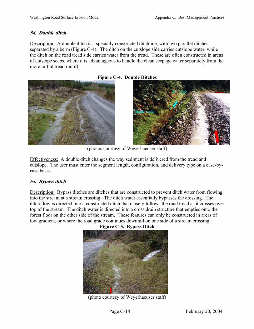
Washington Road Surface Erosion Model Appendix C. Best Management Practices
54. Double ditch
Description: A double ditch is a specially constructed ditchline, with two parallel ditches separated by a berm (Figure C-4). The ditch on the cutslope side carries cutslope water, while
reas
Figure C-4. Double Ditches
Effectiveness:
the ditch on the road tread side carries water from the tread. These are often constructed in aof cutslope seeps, where it is advantageous to handle the clean seepage water separately from themore turbid tread runoff.
(photos courtesy of Weyerhaeuser staff)
A double ditch changes the way sediment is delivered from the tread and c must enter the segment length, configuration, and delivery type on a case-by-case basis. utslope. The user
55. Bypass ditch
Description: Bypass ditches are ditches that are constructed to prevent ditch water from flowinto the stream at a stream crossing. The ditch water essentially bypasses the crossing. The ditch flow is directed into a constructed ditch that closely follows the road tread as it crosses over top of the stream. The ditch water is directed into a cross drain structure that empties onto the forest floor on the
ing
other side of the stream. These features can only be constructed in areas of low gradient, or where the road grade continues downhill on one side of a stream crossing.
(photo courtesy of Weyerhaeuser staff)
Figure C-5. Bypass Ditch
Bank water
Clean water
24” pipe
Page C-14 February 20, 2004
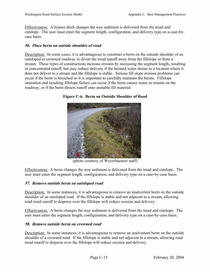
Washington Road Surface Erosion Model Appendix C. Best Management Practices
Effectiveness: A bypass ditch changes the way sediment is delivered from the tread and cutslope. The user must enter the segment length, configuration, and delivery type on a case-by-case basis.
56. Place berm on outside shoulder of road
Description: In some cases, it is advantageous to construct a berm on the outside shoulder ooutsloped or crowned roadway to divert the tread runoff away from the fillslope or from a stream. These types of constructions increase erosion by increasing the
f an
segment length, resulting in concentrated runoff, but may reduce delivery if the bermed water drains to a location where it
n and resulting fillslope failure can occur if the berm causes water to remain on the roadway, or if the berm directs runoff onto unstable fill material.
Figure C-6. Berm on Outside Shoulder of Road
does not deliver to a stream and the fillslope is stable. Serious fill slope erosion problems can occur if the berm is breached so it is important to carefully maintain the berms. Fillslope saturatio
(photo courtesy of Weyerhaeuser staff)
Effectiveness: A berm changes the way sediment is delivered from the tread and cutslope. The user must enter the segment length, configuration, and delivery type on a case-by-case basis.
D
57. Remove outside berm on outsloped road
escription: In some instances, it is advantageous to remove an inadvertent berm on the outside shoulder of an outsloped road. If the fillslope is stable and not adjacent to a stream, allowing road tread runoff to disperse over the fillslope will reduce erosion and delivery.
Effectiveness: A berm changes the way sediment is delivered from the tread and cutslope. The user must enter the segment length, configuration, and delivery type on a case-by-case basis.
58. Remove outside berm on crowned road
Description: In some instances, it is advantageous to remove an inadvertent berm on the outside shoulder of a crowned road. If the fillslope is stable and not adjacent to a stream, allowing road tread runoff to disperse over the fillslope will reduce erosion and delivery.
Page C-15 February 20, 2004

Washington Road Surface Erosion Model Appendix C. Best Management Practices
Effectiveness: A berm changes the way sediment is delivered from the tread and cutslope. The user must enter the segment length, configuration, and delivery type on a case-by-case basis.
Description:
C.6 Sediment Trapping BMPs
60. Protect drainage structure outfall with rip rap
Installing rip rap at a culvert outfall reduces erosion and gullying at the downhill side of the culvert outlet. Energy dissipaters such as rip rap or logs can also slow the velocity of water, resulting in deposition of sand and coarser-grained sedim
Figure C-7. Rip Rap Protection at Culvert Ou
ents.
tfall
(Photo courtesy of Weyerhaeuser staff)
Effectiveness: Few studies on the effectiveness of outfall protection on sediment delivery exist. One study by Grace (2002) found rip rap reduced sediment concentration in runoff to 50 percent of inflow concentration.
61. Install settling basins
Description: Settling basins within ditchlines or at culvert outfalls are often used to trap sediment and reduce delivery to waterways. The size and placement of the settling basin is ofteconstrained by available area and hillslope gradients. Settling basins are most effective in areasof sandy or coarse-silty soil since these particles settle out much more quickly than smaller si
n
lt or clay-sized particles. The settling b all particles increases rapidly with decreas es the settling basins are properly sized so they do , and they are maintained/cleaned often enough to retain theffectiveness of settling basins nuals (e.g., Goldman et al. 1986).
Effectiveness:
asin size necessary to trap sming grain size. The effectiveness listed in Table C-1 assum
not fill with sediment during large stormseir design capacity. Design specifications and
can be found in erosion control ma
on the effectiveness of settling basins is ofban areas where they are mo
a few studies, wh widely with inflowing
n configuration. NCASI (2002) summarized data from
Literature ten the result of testing at construction sites or in ur re frequently used. Settling basins have been tested along forest roads in ich found they were most effective in trapping particles over 0.02 mm. Trap efficiencies varied sediment load, grains size, and basi settling basin studies and
Page C-16 February 20, 2004

Washington Road Surface Erosion Model Appendix C. Best Management Practices
concluded trap efficiencies ra 2) found settling basins sulting
percent trap efficiency. Assuming settling basins are properly sized so they do not overtop during large storms, an 85 percent trap efficiency was assigned to this BMP, resulting in 1 ivering to streams.
62. Install silt fen
Description:
nged from 52 to 96 percent. Grace (200were effective during small storms, but not during large storms when they overflowed, rea net trapping efficiency of 10 percent, similar to the results of a study by Bilby et al. (1989) showing a 19
5 percent of the calculated erosion amount del
Figure C-8. Settling Basins
Fish stream
Fish
(photos courtesy of Weyerhaeuser staff)
ces/hay bales at outfall or in ditchline
ilt fences or hay bales in ditchlines or at culved to a stream. Installation
in contact with the ground surface or that hanufacturer instructions for silt fences, or con
oldman et al. 1986).
Installing s ert outfalls can trap sediment, reducing the amount deliver procedures are important. Hay bales or silt fences that are not ave gaps between bales are not effective. Follow m sult an erosion control manual for proper techniques (e.g., G
Effectiveness: There is limited data on the effectiveness of silt fences or hay bales in forest road
e and installation techniques. An average 25 percent reduction was used for this BMP (0.75 d
settings. Grace (2002) found sediment fences reduced sediment concentrations in runoff by 27 percent. It is likely that effectiveness of these measures varies greatly depending upon grain siz
elivery factor).
63. Vegetate/rock ditch
Description: Vegetation or rock in the ditchline reduces erosion of the ditch and also slows water, allowing sediment in the runoff to be deposited. If the ditch is regraded frequently, this
Effectiveness:
BMP may not be effective.
No specific papers showing the effectiveness of rocking or vegetating ditches on trapping sediment were found.
Page C-17 February 20, 2004
Washington Road Surface Erosion Model Appendix C. Best Management Practices
64. Filter windrow at culvert outfall
Description: Filter windrows are piles of slash, logs, and/or brush that are commonly placed ll side of fillslopes to trap eroded sediment. Filter
windrows or slash can also be left at culvert outfalls to dissipate energy and trap sediment.
Effectiveness:
parallel to the roadway at the downhi
The effectiveness of filter windrows at shortening delivery distances at the base
filter windrows at culvert outfalls were found.
65. Curbs/splash guards on bridges
Description:
of fillslopes has been documented by Swift (1985, see also Figure A-6), and number of obstructions has been positively correlated with travel distances at culvert outfalls (Megahan and Ketcheson 1996). However, no specific studies on the effectiveness of
Installing curbs and splash guards on bridges reduces the amount of sedim splashed off the bridge and into the stream as traffic crosses the bridge.
No published research on the numerical effects of installinuce surface erosion were found.
hat are location
ent-laden water that is
Effectiveness: g curbs or splash guards on bridges to red
C.7 Whole Road BMPs
70. Decommission road
Description: Roads t s (e.g., parallel to a stream) may be candidates fo used or maintained any
, to pulling back oversteepened fillslopes, to re-contouring of the e natural profile and revegetating the area.
no longer used or are constructed in poorr decommissioning. Often roads are not
more, resulting in revegetation, but the road prism and drainage structures are left in place which can result in culvert blowouts or fillslope failures. In some cases, more active road deconstruction measures are taken. These can range from pulling drainage structures and reshaping stream crossingsntire road prism to a more
Effectiveness: The effectiveness of decommissioning depends upon the hazards associatethe old road and the degree of treatment. The factors assigned to this BMP include changing the traffic factor to 0.1 (no traffic), changing the configuration to outsloped and the cutslope height to 0 (assuming road prism regraded) and changing the surfacing to grass (0.5). Different levels of decommissioning may require the use of a Custom BMP.
C.8 Developing Custom BMPs
The road surface erosion model application allows users to create Custom BMPs to model specific measures used on their roads. These BMPs can cover the full range of model factors shown in
d with
Table C-1. The user should be prepared to document any numerical values for the different factors based on road research or measurements for reviewers of model output.
Methods for entering Custom BMPs are described in Chapter 5 of the User’s Manual. Guidelines for developing BMPs are provided below.
Page C-18 February 20, 2004

Washington Road Surface Erosion Model Appendix C. Best Management Practices
Determine the portion(s) or road erosion factors the BMP changes. Most BMPs alter only onefactor, but some may alter more than one. You should have a clear understanding of how the factors you will be modifying were derived. Reference the appropriate section of this technicreport so that you can enter a reasonable value for the factor altered by your Custom BMP.
Custom Traffic Factors
al
Custom traffic factors are entered program. This screen allows
l
ge 1979). Rain w
on a separate screen within theyou to enter a separate traffic factor for each menter BMPs related to seasonal traffic restrictionchange in road use (e.g., traffic associated wi
The model determines a weighted average tramultiplying the traffic levels during each mrainfall occurring during that month, and summtraffic in each month by the percent of rainfall researchers that traffic during rainy weather greatly increaseSullivan and Duncan 1981, WooldridAn example of this process is shown in Table C-2.
Table C-2. Example traffic factor
onth of the year. This process can be used to s or to determine the effects of a short-term
th a single harvest unit or group of units).
ffic value for each custom traffic BMP by onth of the year by the associated percent of the tota
ing the result for 12 months. This weights the in that month, following the findings by several
s erosion (Reid and Dunne 1984, ithout traffic results in much less erosion.
(Haul only during summer, Jun-Oct) Month Jan Feb Mar Apr May Jun Jul Aug Sep Oct Nov Dec Percent of total 2% 3% 5% 20% 20% 10% 2% 2% rainfall
1% 10% 20% 5%
Traffic use
L (1)
L (1)
L (1)
L (1)
L (1)
M (10)
M (10)
M (10)
M (10)
M (10)
L (1)
L (1)
factor (sum of
row) Percent rainfall times 0.02 0.03 0.05 0.2 0.2 1 0.2 0.2
Weighted average traffic
use 0.1 1 0.2 0.05 3.25
factor
In this example, the road is used for haul during the months of June-October at a moderate tlevel (traffic factor
raffic 10). The rest of the year, the road is used only for light administrative use
(occasional pickups). The weighted average traffic factor (3.25) will be used in the model run.
The user need only to enter the traffic use for each month of the year. The model contains
t -9.
information on the monthly distribution of rainfall for each T/R Section in the state. The distribution of rainfall (snowfall water equivalent subtracted from total precipitation) throughouthe year is shown in Figure C
Page C-19 February 20, 2004
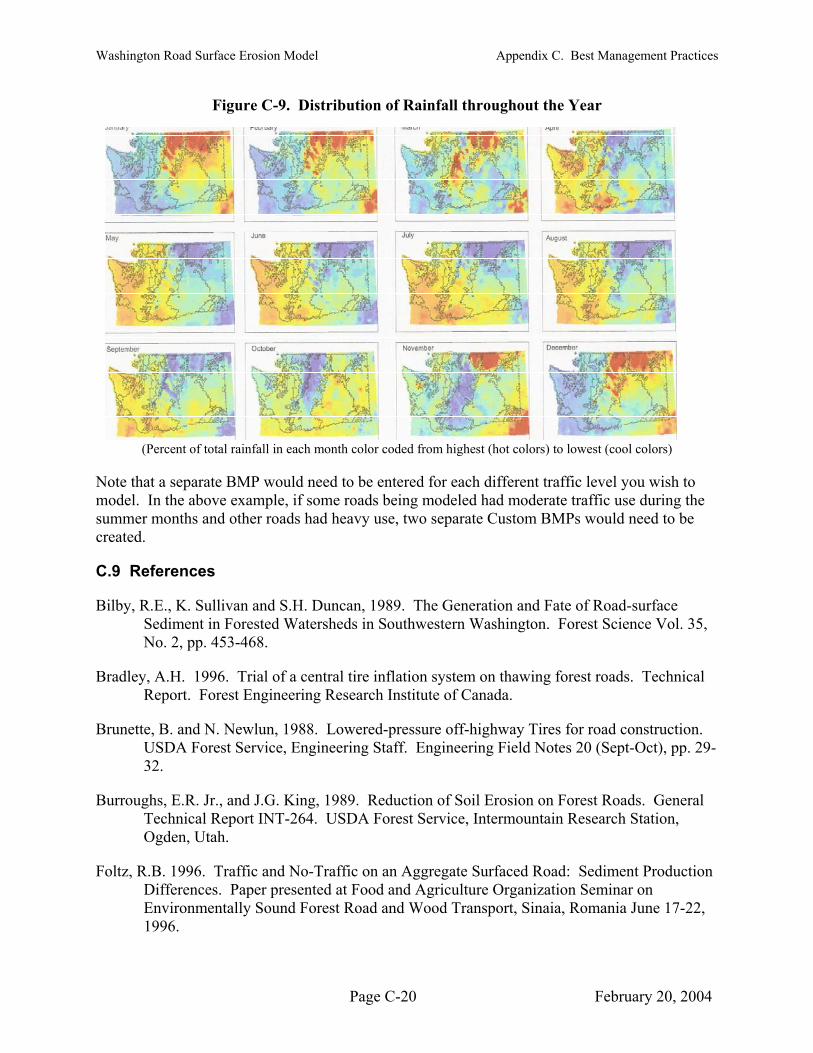
Washington Road Surface Erosion Model Appendix C. Best Management Practices
Fi ure C-9. Distribug tion of Rainfall throughout the Year
each month color coded from highest (hot colors) to lowest (cool colors)
N would need to be entered for each different traffic level you wish to model. In the above example, if some roads being modeled had moderate traffic use during the
5,
Field Notes 20 (Sept-Oct), pp. 29-32.
Burroughs, E.R. Jr., and J.G. King, 1989. Reduction of Soil Erosion on Forest Roads. General
ction Differences. Paper presented at Food and Agriculture Organization Seminar on
17-22,
(Percent of total rainfall in
ote that a separate BMP
summer months and other roads had heavy use, two separate Custom BMPs would need to be created.
C.9 References
Bilby, R.E., K. Sullivan and S.H. Duncan, 1989. The Generation and Fate of Road-surfaceSediment in Forested Watersheds in Southwestern Washington. Forest Science Vol. 3No. 2, pp. 453-468.
Bradley, A.H. 1996. Trial of a central tire inflation system on thawing forest roads. Technical Report. Forest Engineering Research Institute of Canada.
Brunette, B. and N. Newlun, 1988. Lowered-pressure off-highway Tires for road construction. USDA Forest Service, Engineering Staff. Engineering
Technical Report INT-264. USDA Forest Service, Intermountain Research Station,Ogden, Utah.
Foltz, R.B. 1996. Traffic and No-Traffic on an Aggregate Surfaced Road: Sediment Produ
Environmentally Sound Forest Road and Wood Transport, Sinaia, Romania June1996.
Page C-20 February 20, 2004
Washington Road Surface Erosion Model Appendix C. Best Management Practices
Foltz, R. B., and Burroughs, E.R. Jr., 1990. Sediment Production from Forest Roads with WheeRuts. In: Watershed Planning and Analysis; Proceedings of a Symposium, July 9-11 1989, Durango CO. ASCE, pp. 266-275.
l
Foltz, R.B. and W .J. Elliot, 1997. Effect of Lowered Tire Pressures on Road Erosion. rch Record No. 1589, pp. 19-25.
opes in North Alabama. In: Seventh International Conference on Low Volume Roads. Volume
. -
Measures for Silvicultural Operations. Unpublished draft Technical Bulletin. Research Triangle Park, N.C.: National Council for
R T n 8 t u F R S e ae es
Seyedbagheri, K. 1996. Idaho Forestry Best Manageme ra es: mp tion Ren r E tiv ss. D r I i ea St , Gec al or T- -3 8
S n a 8 ed nt d Road Surfaces in ResponseTruck Traffic and Rainfall. Weyerhaeuser Technical Report 042-4402.80.
pany, Technical Center, Tacoma, WA 98477.
Swift, L.W. Jr., 1985. Soil Losses from Roadbeds and Cut and Fill Slopes in the Southern
Wooldridge, D.D., 1979. Suspended Sediment from Truck Traffic on Forest Roads, Meadow f
Transportation Resea
Goldman, S.J., K. Jackson, T.A. Bursztynsky, 1986. Erosion and Sediment Control Handbook.Mc-Graw Hill: New York.
Grace, J.M., III. 1999. Erosion Control Techniques on Forest Road Cutslopes and Fillsl
2; Transportation Research Record 1652; pp. 227-234.
Grace, J.M., III. 2002. Sediment Transport Investigations on the National Forests of AlabamaIn; Proceedings of the International Erosion Control Association Conference 33, Feb. 25Mar 1, 2002, Orlando, FL, pp. 347-357.
NCASI, 2000. Handbook of Control and Mitigation
Air and Stream Improvement, Inc.
eid, L.M. and . Dun e, 19 4. Sedimen Prod ction from orest oad urfac s. W ter
search eneral
R sourc Research Vol. 20, No. 11, pp. 1753-1761.
nt Pnterm
cticounta
Con Res
ilarch
ofationo Thei
hnicffec
Repenet IN
USGTR
A Fo39.
est Se9 pp.
rviceT
ullivan,
Weyerhaeuser Com
K.O. a d S.H. Dunc n, 19 0. S ime Yiel from to
Appalachian Mountains. Southern Journal of Applied Forestry, Vol. 8 No. 4, pp. 209-213.
and Coal Creeks. Water Quality Planning. Office of Water Programs, Department oEcology, Olympia, WA. 79-5a-3.
Page C-21 February 20, 2004

Washington Road Surface Erosion Model Appendix C. Best Management Practices
Page C-22 February 20, 2004

Appendix D. Field Testing Results


Appendix D. Field Testing Results
Contents
D.1 Introduction..................................................................................................................... D-4 D.2 Methods........................................................................................................................... D-4
D.2.1 Field Methods ......................................................................................................... D-4 D.2.2 Statistical Analysis.................................................................................................. D-5
D.3 Study Areas and Field Testers ........................................................................................ D-7 D.3.1 Stossel Creek........................................................................................................... D-7 D.3.2 Forks ....................................................................................................................... D-9 D.3.3 Thrash Creek......................................................................................................... D-11
D.4 Results........................................................................................................................... D-12 D.4.1 Identification of segments and measurement precision for total length ............... D-13 D.4.2 Predicted sediment yields ..................................................................................... D-14 D.4.3 Precision of model inpD.4.4 Sensitivity Analysis of
D.5 Summary ....................................................................................................................... D-21 D.6 Recommendations......................................................................................................... D-22 D.7 References..................................................................................................................... D-22
List of Tables
Table D-1. Characteristics of Stossel Creek field testers........................................................... D-8 Table D-2. Characteristics of Forks field testers. .................................................................... D-10 Table D-3. Characteristics of Thrash Creek field testers. ........................................................ D-12
List of Figures
Figure D-1. Mean and range of segment counts by road sections........................................ D-26 Figure D-2. Length of road assigned to delivery classes by observers and road section
at the Thrash Creek site..................................................................................... D-26 Figure D-3. Length of road assigned to delivery classes by observers and road section
at the Stossel Creek site .................................................................................... D-27 Figure D-4. Length of road assigned to delivery classes by observers and road section
at the Forks site ................................................................................................. D-27 Figure D-5. Coefficient of variation for sediment delivery percent and total length for
Thrash Creek road sections............................................................................... D-28 Figure D-6. Coefficient of variation for sediment delivery percent and total length for
Stossel Creek road sections............................................................................... D-28 Figure D-7. Coefficient of variation for sediment delivery percent and total length for
Forks road sections ........................................................................................... D-29 Figure D-8. Predicted sediment yields by road and observer, Thrash Creek site................. D-29 Figure D-9. Predicted sediment yields by road and observer, Stossel Creek site ................ D-30 Figure D-10. Predicted sediment yields by road and observer, Forks site ............................. D-30
ut variables........................................................................ D-15 model inputs .................................................................... D-19
Page D-1 February 20, 2004

Washington Road Surface Erosion Model Appendix D. Field Testing Results
Figure D-11. Standard deviation vs. mean of predicted sediment yield for individual road segments at the Thrash Creek site............................................................. D-31
Figure D-12. Standard deviation vs. mean of predicted sediment yield for individual road segments at the Stossel Creek site ............................................................ D-31
Figure D-13. Standard deviation vs. mean of predicted sediment yield for individual road segments at the Forks site ......................................................................... D-32
Figure D-14. Standard deviation of predicted sediment yield by experience level for the Thrash Creek site .............................................................................................. D-32
Figure D-15. Variability in Length by segment and road, Thrash Creek site ........................ D-33 Figure D-16. Variability in Length by segment and road, Forks site..................................... D-33 Figure D-17. Variability in Tread Width by segment and road, Thrash Creek site ............... D-34 Figure D-18. Variability in Tread Width by segment and road, Stossel Creek site ............... D-34 Figure D-19. Variability in Tread Width by segment and road, Forks site............................ D-35 Figure D-20. Variability in Ditch Width by segment and road, Thrash Creek site................ D-35 Figure D-21. Variability in Ditch Width by segment and road, Stossel Creek site................ D-36 Figure D-22. Variability in Ditch Width by segment and road, Forks site ............................ D-36 Figure D-23. Variability in coefficient of variation for continuous variables by road
section and location........................................................................................... D-37 Figure D-24. Variability in Road Gradient by segment and road, Thrash Creek site ............ D-37 Figure D-25. Variability in Road Gradient by segment and road, Stossel Creek site ............ D-38 Figure D-26. Variability in Road Gradient by segment and road, Forks site......................... D-38 Figure D-27. Variability in Delivery by segment and road, Thrash Creek site...................... D-39 Figure D-28. Variability in Delivery by segment and road, Stossel Creek site ..................... D-39 Figure D-29. Variability in Delivery by segment and road, Forks site .................................. D-40 Figure D-30. Variability in Configuration by segment and road, Thrash Creek site ............. D-40 Figure D-31. Variability in Configuration by segment and road, Stossel Creek site ............. D-41 Figure D-32. Variability in Configuration by segment and road, Forks site.......................... D-41 Figure D-33. Variability in Surfacing by segment and road, Thrash Creek site .................... D-42 Figure D-34. Variability in Surfacing by segment and road, Stossel Creek site.................... D-42 Figure D-35. Variability in Surfacing by segment and road, Forks site................................. D-43 Figure D-36. Variability in Cut Cover by segment and road, Thrash Creek site ................... D-43 Figure D-37. Variability in Cut Cover by segment and road, Stossel Creek site................... D-44 Figure D-38. Variability in Cut Cover by segment and road, Forks site................................ D-44 Figure D-39. Variability in Cut Height by segment and road, Thrash Creek site .................. D-45 Figure D-40. Variability in Cut Height by segment and road, Stossel Creek site.................. D-45 Figure D-41. Variability in Cut Height by segment and road, Forks site............................... D-46 Figure D-42. Variability of road properties at Thrash Creek site (class variables)................ D-46 Figure D-43. Variability of road properties at Stossel Creek site (class variables)................ D-47 Figure D-44. Variability of road properties at Forks site (class variables) ............................ D-47 Figure D-45. Overall average values and statistical differences of VI for categorical
input variables................................................................................................... D-48 Figure D-46. Sensitivity Analysis of WARSEM variables, Thrash Creek site...................... D-48 Figure D-47. Sensitivity Analysis of WARSEM variables, Stossel Creek site...................... D-49 Figure D-48. Sensitivity Analysis of WARSEM variables, Forks site .................................. D-49 Figure D-49. Average sensitivity ranking of WARSEM variables for all sites ..................... D-50
Page D-2 February 20, 2004

Washington Road Surface Erosion Model Appendix D. Field Testing Results
List of Plates
Plate D-1. Stossel Creek mainline road. .................................................................................... D-7 D D
Plate D-4. FPlate D-5. F
DPl . T
Plate -2. Stossel Creek spur road. ........................................................................................... D-8 Plate -3. Forks 5000 mainline road. ........................................................................................ D-9
orks 5050 road. ..................................................................................................... D-10 orks 5060 unused road.......................................................................................... D-10
Plate -6. Thrash Creek 2000 road.......................................................................................... D-11 ate D-7 hrash Creek 2100 road.......................................................................................... D-12
Page D-3 February 20, 2004

Washington Road Surface Erosion Model Appendix D. Field Testing Results
Appendix D. Field Testing Results
D.1 Introduction
One of the objectives for preparing a standardized road surface erosion method was to result in repeatable calculations of road surface erosion. The WARSEM
develop a tool that would
ork for calculating
een observers cove
M
DNR staff to large landowners to small landowners.
database application is one step toward standardization, since it provides a standard framew erosion (removes the potential for errors that may occur if each modeler
developed their own spreadsheet for calculations).
A second part of the standardization process involves developing protocols for measuring road characteristics on the ground that can be duplicated by different observers. The field protocols discussed in Chapter 4 of the WARSEM manual attempt to describe how to measure and categorize each of the model input parameters.
Based on the assumption that most people using the model would be untrained, a series of three field tests using largely untrained observers was carried out to test the variability betw
ring the same road segments. The range of characteristics measured by the different observers at each site was also used to show how sensitive the WARSEM model is to the different input parameters. These data and analyses are valuable to help model users and those interpreting model results understand which road characteristics influence the results and the amount of variability expected in model predictions of road surface erosion.
D.2 Methods
Three test sites were chosen across western Washington to sample different physiographic regions as well as different road building styles. The timing of the testing (February) limited the test to lower-elevation sites in western Washington since other parts of the state were snow covered at that time. The sites included:
Stossel Creek (located just east of Duvall in the central Cascade foothills)
Forks (north of the town of Forks, just south of Lake Ozette on the Olympic Peninsula)
Thrash Creek (just south of Pe Ell in the Willapa Hills area)
D.2.1 Field ethods
At each study site, two to three road sections were chosen that included both delivery and non- delivery portions. The test sections were not chosen randomly, but were selected to include
nt, mid-different types of roads (mainline, secondary, spur) and slope positions (stream-adjaceslope) to test the field measurements in a variety of settings.
Field testers were chosen based on willingness and availability, to reflect a spectrum of people ranging from those who had extensive experience doing road surface erosion studies and inventories to individuals who had no previous experience. This was done to represent the variety of people who may be using the methods to perform inventories on road systems, from W
Page D-4 February 20, 2004

Washington Road Surface Erosion Model Appendix D. Field Testing Results
Prior to the field test, all of the field testers were given a copy of the February 3, 2000 version of rotocol section from the manual (Chapter 4) and a copy of Appendix C (Best
Management Practices) as well as blank field forms and reference sheets from Appendix B.
ppropriate geologic erosion category at each site and told to make their best guess at traffic rates, but these items were held constant during the analysis since the field protocol indicates that these variables will be determined based on discussions with a geologist and the local road or land manager. Testers were allowed to use whatever measuring technology they chose (pacing, tape, measuring wheel, clinometer, etc.).
The field test consisted of two parts. First, the testers were instructed to walk along the entire test section and break it into segments based on the instructions in the field protocols. They were told to write down the length of each segment and the delivery type for each segment (direct to stream, within 100 feet of a stream, within 200 feet of a stream, or no delivery). This was to determine the ability of testers to segment the road and determine delivery type.
Following the first walk down the road, all segment start and end points were selected by the person supervising the test and marked with flagging. The testers then made a second pass along the road and collected all information on the standard field form for each of these segments. Segment length on the pre-determined segments was collected at the Forks and Thrash Creek sites, but not at the Stossel Creek site. The pre-determined segments were used to determine the repeatability of measurements by different testers viewing the same road segment.
D.2.2 Statistical Analysis
All data on field forms collected at each of the three test sites were entered into Excel spreadsheets into two groups; one group consisted of the initial field test information designed to evaluate the variability of road segment length and delivery and the second group designed to evaluate the variability of model variables on pre-determined road segments. Sediment yield values were calculated using WARSEM for each road segment for each of the observers.
Statistical analysis of the segment length & delivery data consisted of contingency tables and/or charts showing the total length of road in each sediment delivery class for each observer along with the mean, standard deviation and coefficient of variation (CV = standard deviation/mean) value across observers for each sediment delivery class.
Statistical analysis of the data collected to evaluate the variability of model variables was different depending on whether the variable was continuous or categorical. Continuous variables are those whose value could be any number; segment length is an example of a continuous variable. Categorical variables are those that an observer must make a selection from a choice of values, such as surfacing or cutslope height.
the draft field p
Note that improvements to descriptions in Chapter 4 have been made subsequent to the field testing based on the results of the test.
At the field site, the testers were instructed that the purpose of the test was to examine the repeatability of the measurements and to determine if the field protocol adequately described how to measure the different parameters. The testers were not allowed to ask questions about the field protocols or to discuss their results among themselves. The testers were told the a
Page D-5 February 20, 2004

Washington Road Surface Erosion Model Appendix D. Field Testing Results
For continuous variables ndard deviation were calculated across observers for each road segment, sample road and sample site. In addition, a
ated for each road segment and test road to provide a method to compare variability between areas.
ncy of
pare are statistic but utilizes the total number of
classes as the denominator in order to avoid dividing by zero. The VI value is directly
a mean, maximum value, minimum value and sta
mean CV value was calcul
Contingency tables were used to evaluate categorical variables and consisted of the frequeoccurrence of each variable class for each road segment summarized by sample roads and test site. A variability index (VI) value was developed to provide a quantitative value to comlocations. The VI is somewhat similar to the chi squ
proportional to the amount of variance between observers. VI is calculated as follows:
[ ]frequency class expectedfrequency class actualni
1i
2i∑ − i
=VI N
Where: i = the individual class frequency values
n = the number of classes
N = the total number of observers.
=
=
ent all observers would select the same class and all other classes would . For example, in the case of the Forks site with seven observers, one class
ro.
f 4, sloped road configuration classes respectively. The
class w n is crowned and apply the expected value of seven to that class and expected values of zero to all other classes
VI = [(4-7) + (2-0) + (1-0) ] / 7 = [9 + 4 + 1] / 7 = 2
ompare variables. A one-way
analysis of variance was used to determine statistical differences between VI values for input
s. Rather, the maximum and minimum value for each input variable was used to calculate sediment yield holding all other values at their
With complete agreemshow no observationswould show an expected frequency of seven with the rest zero, resulting in a VI value of zeHowever, this does not occur in most instances. When variation occurs, the assumption is made that the classification that is most probably correct is the one reported most frequently. For example using the Forks data, assume the seven observers reported actual class frequencies o2 and 1 for the crowned, insloped and out
ith the highest frequency is crowned so we assume the correct classificatio
. Substituting in the VI equation above gives:
2 2 2
In the case of equal high actual frequency values, one of the high class values is arbitrarily selected for pairing with the expected class frequency of seven and all other expected class frequencies were assumed to be zero. Graphs were developed to show differences in VI valuesby road segments and roads for each of the study sites and to c
variables.
Finally, a sensitivity analysis was used to illustrate the relative influence of individual inputvariables on sediment yield predictions. Most of the input variables are categorical so it is not possible to illustrate sensitivity with continuous function
Page D-6 February 20, 2004

Washington Road Surface Erosion Model Appendix D. Field Testing Results
overall average value for the test site. The range in predicted sediment yield (maximum minus minimum) was then used to compare variable sensitivity. Graphs were developed to comparesensitivity ratings between sites.
D.3 Study Areas and Field Teste
rs
ation r
nketed by till (Qgt) with Eocene volcanic rocks (Ev)
ce p Tribe).
Weather on both days was sunny. There were no active timber sales in the area at the time of the
; n
he east side of the valley bottom (Plate D-1). Several small streams and seeps crossed the road. The road
of its length, making determination of drainage direction difficult.
The following sections describe the setting at each of the three test sites and general informabout the group of testers at each site. A few testers were present at more than one site, but fothe most part the group of testers was unique at each site.
D.3.1 Stossel Creek
The Stossel Creek site is located in the Marckworth State Forest, just east of the city of Duvallin the Cascade foothills (T26N R7E, Sections 12, 13, and 24). The Marckworth State Forest is managed by the Washington Department of Natural Resources. Elevations at the study site ranged from 500 to 800 feet. The site is blaforming higher hillsides (Dragovich et al. 2002). Vegetation is typical of lowland Douglas fir forests, with mixed conifer/deciduous stands in riparian and disturbed areas. The Stossel Creek stream valley is U-shaped in the study area, with steep sides and a broad, flat valley bottom dominated by low-gradient streams with numerous ponds and wetlands. Field testing took plaon February 7, 2003 (main group) and February 12, 2003 (3 testers from the Tulali
field test.
Two road segments were selected for testing: a 1.4-mile stretch of the mainline ST-5000 roadand a 0.8-mile long stretch of the gated spur road heading east from the ST-5000 road in Sectio24. The mainline road section chosen for the study paralleled Stossel Creek on the west valley wall for approximately one mile, then crossed the creek and paralleled the creek on t
surface was nearly flat for much
Plate D-1. Stossel Creek mainline road.
The spur road crossed Stossel Creek and a small tributary in the broad valley bottom, then steeply climbed the hillside on the east side of Stossel Creek and crossed the upper end of the
Page D-7 February 20, 2004

Washington Road Surface Erosion Model Appendix D. Field Testing Results
same tributary near the end of the test segment (Plate D-2). The road was gated to prevent casuause by cars and trucks. A settling basin and several hay bales had been installed near the lower tributary crossing to help trap sediment from the road prism.
l
Plate D-2. Stossel Creek spur road.
Two groups of testers col ation at the Stossel Creek site. The main group collected data on February 7, and included nine testers. The second group included staff members from the Tulalip nts on February 12. The testers included foresters, geologists, and hydrologists from private consulting firms, the WDNR,
lected road inventory inform
Tribe who measured the road segme
CMER, the Tulalip Tribe, and the Resource Technology Institute at the University of Washington (Table D-1). Eight of the testers had no experience doing road inventories; one tester had limited experience with road surveys, and two testers (the prime contractors for the current study) had extensive road inventory experience.
Table D-1. Characteristics of Stossel Creek field testers.
Affiliation Experience Measuring Equipment Used (ocular estimate unless noted)
Consultant Geologist – 13 years doing road erosion studies
Paced distance/ width; clinometer slope
Consultant Forest road researcher Paced distance/ width, clinometer slope
Consultant Forester – first road inventory survey
Paced distance/ width, clinometer slope
UW Resource
Technology Institute (small landowner advocate group at UW)
First road inventory survey Paced distance/width; clinometerslope
UW Resource Technology
Laser rangefinder for Institute Not noted distance/width
Consultant Forester – some experience with road surveys, but none segmenting roads for delivery
Paced distance; tape width
WDNR First road inventory survey String box for width/distance
Page D-8 February 20, 2004

Washington Road Surface Erosion Model Appendix D. Field Testing Results
Affiliation Experience Measuring Equipment Used (ocular estimate unless noted)
CMER (NWIFC) Geologist – no road experience Paced distance/ width Tulalip Tribe Not noted Paced distance/ tape width Tulalip Tribe Not noted Paced distance/ width
Tulalip Tribe Forest engineering/hydrology background.
Note: did not count wetlands as a stream when determining delivery
D.3.2 Forks
The Forks test site is located in the Dickey River and South Creek drainages, just south of OzetteLake on the Olympic Peninsula (T29N R15W, Sections 14 and 23). The area is managed by Rayonier. Elevations at the study site ranged from 200 to 400 feet. The site is blanketed by glacial drift(Qgd) and outwash (Qgo) with Oligocene-Eocene marine sedimentary rocks (ΦEm) forming higher hillsides (Dragovich et al. 2002). Vegetation is typical of lowland Douglas fir forests, with mixed conifer/deciduous stands in riparian and disturbed areas. The area has gentlehills and broad, low gradient stream valleys with numerous ponds and wetlands. Field testing took place on February 12, 2003. The weather was sunny. There were no active timber sales in the area at the time of the field test.
Three road segments were selected for testing: a 0.9-mile stretch of the mainline 5000 road; a 0.6–mile str
etch of the 5050 road and a 0.3-mile long stretch of the unused 5060 road. The mainline 5000 road section chosen for the study paralleled Coal Creek on the west side of the valley (Plate D-1). The 5000 road was a through cut for much of the inventoried length, with a ditch on each side of the road. During the survey, it was receiving use primarily by pickups and cars. The road surface was nearly flat for much of its length, making determination of drainage direction (and thus road segment length) difficult.
Plate D-3. Forks 5000 mainline road.
The 5050 road is a midslope road with numereceives some use, but is partially vegetated indicating it does not receive heavy use. The road is
rous small tributary crossings (Plate D-4). The road
generally well maintained with recently placed cross drain culverts.
Page D-9 February 20, 2004
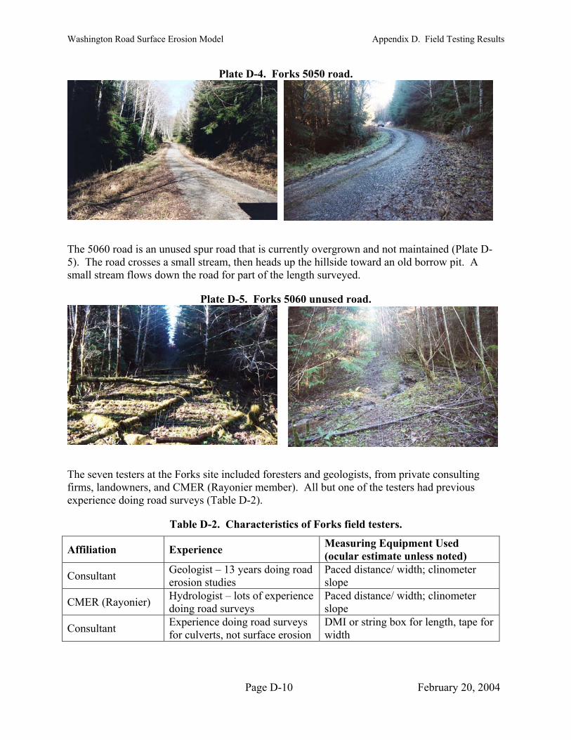
Washington Road Surface Erosion Model Appendix D. Field Testing Results
Plate D-4. Forks 5050 road.
The 5060 road is an unused spur road that is cu5). The road crosses a small stream, then head small stream flows down the road for part of the length surveyed.
rrently overgrown and not maintained (Plate D-up the hillside toward an old borrow pit. A s
Plate D-5. Forks 5060 unused road.
The seven testers at the F private consulting wners, and C r). All bu
experience doing road surveys (Table D-2).
Table D-2. Characteristics of For ters.
Experience Measuring Equipment Used (o
orks site included foresters and geologists, fromfirms, lando MER (Rayonier membe t one of the testers had previous
ks field tes
Affiliation cular estimate unless noted)
Consultant Geologist – 13 years doing road erosion studies
Paced distance/ width; clinometer slope
CMER (Rayonier) Hydrologist – lots of experience doing road surveys
P linometer s
aced distance/ width; clope
idth Consultant Experience doing road surveys for culverts, not surface erosion
DMI or string box for length, tape for w
Page D-10 February 20, 2004

Washington Road Surface Erosion Model Appendix D. Field Testing Results
Ex M(oAffiliation perience easuring Equipment Used
cular estimate unless noted)
Consultant Exfor culverts, not surface erosion
DMI or string box for length, cm pe height
perience doing road surveys linometer slope, calibrated easuring rod for cutslo
Consultant Fow Prester – some experience
ith road surveys aced distance
Consultant Experience doing road surveys for culverts, not surface erosion
DMI or string box for length, tape for width
Rayonier Forester – very little experience doing road surveys
Measuring wheel or pacing for distance/width
D.3.3 Thrash Creek
The Thrash Creek site is located in the Chehalis River watershed south of the city of Pe Ell in tWillapa Hills (T12N R5W, Sections 32 and 33). The site is managed by Weyerhaeuser. Elevations at the study site ranged from 800 to 1,600 feet. The site is underlain by Eocene volcanic rocks of the Crescent Formation (Evc) cut through with intrusive basalt sills and dikes (Eib; Walsh et al. 1987). Vegetation i
he
s typical of lowland Douglas fir forests, with mixed conifer/deciduous stands in riparian and disturbed areas. Stream valleys in the area are V-
, the
-6). Several small streams and seeps crossed the road, with well-defined culverts and cross drains. There was little activity on the road during the road invento ast to access upstream areas.
Plate D-6. Thrash Creek 2000 roa
shaped, with average hillslope gradients of 40 percent. Field testing took place on February 272003). The weather was sunny. There were no active timber sales in the area at the time of field test.
Two road segments were selected for testing: a 0.6-mile stretch of the 2000 road; and a 0.5-mile long stretch of the 2100 road. The 2000 road is a primary road, running parallel and adjacent to Thrash Creek on the north side of the stream (Plate D
ry, but the road had been well used in the p
d.
Page D-11 February 20, 2004
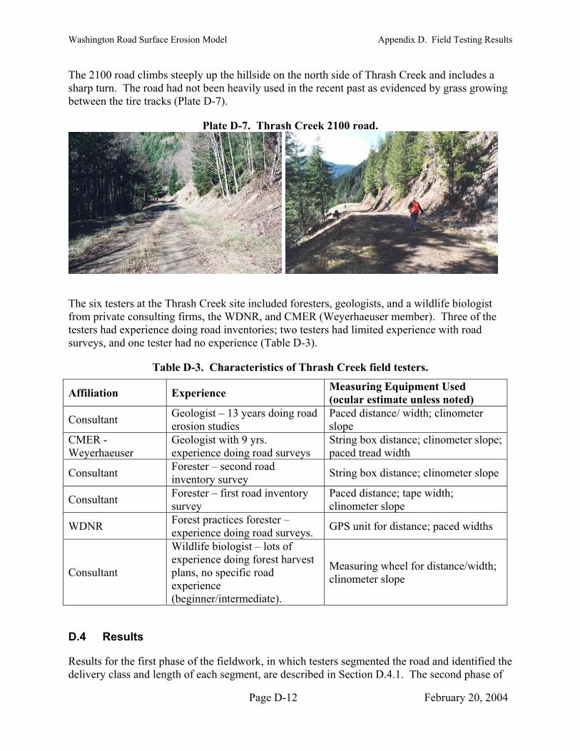
Washington Road Surface Erosion Model Appendix D. Field Testing Results
The 2100 road climbs steeply up hrash Creek and includes a sharp turn. The road had not been heavily used between the tire tracks (Plate D-7).
the hillside on the north side of Tin the recent past as evidenced by grass growing
Plate D-7. Thrash Creek 2100 road.
The six testers at the Thrash C nd a wildlife biologist from private consulting firms, the WDNR, and testers had experience doing road inventories; two testers hasurveys, and one tester had no experience (Tab
Table D-3. Characteristics o
Affiliation Experience
reek site included foresters, geologists, aCMER (Weyerhaeuser member). Three of the
d limited experience with road le D-3).
f Thrash Creek field testers.
Measuring Equipment Used (ocular estimate unless noted) Paced distance/ width; clinometer slope
rveys String box distance; clinometer slope; paced tread width
Consultant Geologist – 13 years doing road erosion studies
CMER - Weyerhaeuser
Geologist with 9 yrs. experience doing road su
Consultant Forester – second road String box distance; clinometer slope inventory survey
Consultant Forester – first road inventory survey
Paced distance; tape width; clinometer slope
WDNR Forest practices forester – e; paced widths experience doing road surveys. GPS unit for distanc
Consultant
Wildlife biologist – lots of ing forest harvest dth; experience do
plans, no specific road experience (beginner/intermediate).
Measuring wheel for distance/wiclinometer slope
D.4 Results
Results for the first phase of the fieldwork, in which testers segmented the road and identified the delivery class and length of each segment, are described in Section D.4.1. The second phase of
Page D-12 February 20, 2004

Washington Road Surface Erosion Model Appendix D. Field Testing Results
the fieldworfrom pre-ma
k required observers to collect all information needed to predict sediment yields rked road segments utilizing the standard field forms. The pre-determined segments
were used to determin nt resent e second m iment
yields between observ e ent precision of individua ) a sensitivity analysis of model input
tification cision for total length
art of the fie a reak it to segments based o he field protoc test sections were
learly marked so all observers were sampling the same length of road. They were told to write egment and the delivery type for each segment (direct to stream = 0 feet of a stream = 35% delivery, or within 200 feet of a stream = 10%
l al
em,
us it is not surprising that there was wide variation in the identification of road segments and the assessment of sediment delivery to streams. Figure D-1 shows the average and
s
e
mber of segments identified amounting to about 80 percent of the average segment count.
Variation in the number of segments identifiedobservers assign similar lengths to order to compare the precision of field obssummarized the length of road assigned to sedimsection for each of the study sites (Figures D-2, D-3 and D-4). direct delivery segments on all of the road sec e fact that all road sections were selected to includconsistent data set was found at the Thrash Crwhere all observers reported a large length of total delivery delivery in some cases. Total road length agre ean of 3,117 feet. All but one observer also recorded somThrash Creek and three of the six observers reported some partial delivery. At the Stossel Creek site, all observers identified some non-delivery road segments on both sample road sections (Figure D-3). In addition, 6 of the 10 observers reported some partial delivery on the 1000 road
e the repeatability of measuremeanalysis in three sections: 1) a coers by road section and sample sit
s over the same segment. We pparison of total predicted sed; 2) an assessment of the measurem
results for th
l model input variables; and 3variables.
D.4.1 Iden of segments and measurement pre
The first p ld test required observers to walkn the instructions in t
long the entire test section and bols. Ends of thein
cdown the length of each s100% delivery, within 10delivery). This was to determine the ability of testers to segment the road and determine delivery type.
For purposes of sediment yield prediction, road segments are defined on the basis of the potentiafor sediment delivery from individual sections of the road. In order to delineate an individuroad segment, field crews must be able to recognize where roads intersect the drainage systthe existence of cross drains and associated paths of direct delivery to channels and the proximityof roads to streams. It is difficult for totally untrained personnel to locate and assess these features. Th
range of segment counts identified by field personnel for the road sections established at the three sample sites. Three of the road sections, the two Thrash Creek sites and the Forks 5060 siteshowed close agreement in the number of road segments identified. The Stossel 2000 site iintermediate in terms of range relative to the mean number of sites. The Forks 5050 and 5000road sites and the Stossel 1000 site have the highest variation in segments identified with a rangin the nu
is not necessarily bad as long as the field the various delivery classes and to the total length of road. In
ervers’ delineations of delivery lengths, we ent delivery classes by observers and road
All observers identified some tions sampled at all sample sites. This reflects th
e at least one channel crossing. The most eek site (Figure D-2) on the 2000 road section
with lesser amounts of partial ed quite well, with little variation around the m
e non-delivery sections on the 2100 road at
Page D-13 February 20, 2004

Washington Road Surface Erosion Model Appendix D. Field Testing Results
and 8 of the 10 observers reported some partial delivery on the 2000 road. Similar levels of variation were found at the Forks site (Figure D-4).
One fact that is apparent in Figures D-2, D-3 and D-4 is that there is wide variation in total length between observers for On the Forks 5060 road, the spread exceeded 100 percent from the high to low valuesStossel Creek sites, the pattern of higher/lower ththe sample road sections were well marked, the dif st be due entirely to errors in measurement of measuring road or segment length; different obswheel, calibrated truck odometer or a laser rangethe precision and accuracy of different measurem the available data because of limited sample sizes error for distance measurement. For example atsecondary roads joined into the primary road with ary road. Some of the observers included these exbeyond the marked boundaries while others did not. This contributed to the higher level of
D-6 k and Stossel Creek
sites (Figures D-5 and D-6). Variability is lowest for the total road length, somewhat greater and about equal for th in 100 feet
s, and gre /in 200 feet delivery and ct that: 1 be minimal variation road direct deli channels f 100 feet delivery segments are easier to define
200 feet deli they are clohat fo fo 0 feet delivery and
non-delivery classes s r the other patterns are still apparent (Figure D-7).
Several field testers co e a ls (Chapter to wetlan considered delivery to a st ry to an obvious
floodplain was consid Discussions with the testers after the ents were co r e
direct delivery and som considered delivery to a floodplain as direct delivery and some did arly defined in the present version of the
ls.
D.4.2 Predicted se
ata from the second phase of the field study were used to calculate sediment yields using hase of the study, observers were asked to evaluate the characteristics of gments using the standard field forms including their own measurements of
the same road section at most locations. . Note that at the Thrash Creek and
an the average is consistent by observer. Since ferences in total length at these two sites mu
length. Observers selected their own method for ervers used pacing, tape, stringbox, measuring finder. The study was not designed to evaluate ent technologies nor is it possible to do so with. However, there is at least one other source of
the Forks site, there were locations where a part of their length draining into the prim
a portions of the road network that extended tr
variability in total road length at this site.
We calculated the coefficient of variation (CV = standard deviation/mean) in order to compare variability of road segment length measurements by delivery classes and sites (Figures D-5,and D-7). General patterns of the variability are clear for the Thrash Cree
e direct delivery and non-delivery classes, greater yet for the w/delivery clasreflect the fa
atest for the w) there should
class. These trends are logical in the total length of the marked
sections; 2) defined for c
very is readily apparent at stream ar from streams; and 4) w/in
rossings; 3) non-delivery is easily
than w/in weakens somew
very segments becauser the Forks data with CV values
ser to the stream. The general trend r both the within 10
omewhat higher howeve
mmented that they were not surds was
fter reading the field protocoream, and if delive4) if delivery
ered direct delivery or not. mpleted indicated that some testemeasurem s considered delivery to wetlands to be did not, and some testers
not. These two situations are cle
diment yields
field protoco
DWARSEM. In this ppre-identified road sesegment length. There were large differences in predicted sediment yields between the three sites, between roads at a given site and between observers (Figures D-8, D-9 and D-10). At an average of 108 t/ac/yr (mean for all observers), the 5000 road section at the Forks site is the Page D-14 February 20, 2004

Washington Road Surface Erosion Model Appendix D. Field Testing Results
largest sediment producer (Figure D-10). This is a mainline road paralleling the creek and is through cut for much of its length with a double ditch. Such roads are very difficult to drain and, coupled with the streamside location, wide tread, and high traffic, results in high sediment yieldThe second highest sediment producer is the 1000 road section at the Stossel site at 41 t/ac/yr(Figure D-9). Although better drained than the 5000 road at the Forks site, this is still a mainlineroad paralleling a creek. Average sediment yields on the remaining study road sections ranfrom a high
a
s.
ge
of 6 t/ac/yr on the 2000 road section at the Thrash Creek site to a low of 1.2 t/ac/yr at the 5060 road section at the Forks site in response to varying site conditions.
There is large variation in average predicted sediment yields between observers at each of the
ion
tely
erience level of observers is one factor that can contribute to large variability in predicted sediment yields. The field study was not designed to test for differences in experience
ch
ce.
ent
We can gain some understanding of how to reduce the variability in sediment yield predictions with
n actual
tor,
the uts
riation
test road sections with about an order of magnitude difference between the lowest and the highest values at most locations. In order to assess the nature of the variance, standard deviatand mean values were calculated comparing observers at each individual road segment for each of the road test sites. Plots of the data show that the standard deviation values are approximaequal to the mean values at all road sections and sample sites (Figures D-11, D-12 and D-13)
The exp
levels on the variability of sediment yield predictions. However, data from the Thrash Creek site do provide some indications of effects. There were six observers at Thrash Creek, three of whicould be nominally classified as having high experience in road erosion assessment and three with low experience. Standard deviation values for the two groups of three were calculated for all road segments on Thrash Creek (Figure D-14). At most road segments, variability for observers with low experience was equal to or greater than for observers with high experienA paired t-test of the values showed that variability was lower for people with high experience (P<0.1). Experience as rated for this test was based on observer’s descriptions of their past activities and does not reflect experience with sediment yield prediction using WARSEM. Thus it is likely that specific training in the use of WARSEM would reduce the variability of sedimpredictions even further for these people as well as others with lower experience levels.
D.4.3 Precision of model input variables
between observers by examining the precision of model input variables. As is necessary any road erosion model, the road in question must be sampled in segments that are assumed to be homogeneous with respect to input variables. Only one descriptor, segment length, is ameasured value subject to normal sampling error. All other road attributes are estimates of average values for the segment. Two of the input variables, precipitation and the geologic facare assigned by WARSEM and are not determined by field personnel7. Traffic levels are normally obtained from land managers, as it is usually impossible to evaluate traffic use in field. The other model inputs are one of two types, continuous or categorical. Only three inpare continuous: segment length; tread width; and ditch width. We use the coefficient of va(CV = standard deviation/mean) to describe variation in continuous variables. Categorical variables differ depending on whether or not the variable classes have a logical numerical
7 Although values for both precipitation and geologic factor can be modified if local conditions observed by qualified field personnel warrant.
Page D-15 February 20, 2004
Washington Road Surface Erosion Model Appendix D. Field Testing Results
ranking. The ranked categorical variables include road gradient, sediment delivery, road cut cover, road cut height and traffic. The unranked categorical variables are road tread configuration and surfacing. We use the variability index (VI) described in the section on statistical analysis above to evaluate variability of all categorical variables.
D.4.3.1 Continuous variables
Segment length CV values for measured segment length by road sections are plotted on Figures D-15 and D-16 for the Thrash Creek and Forks sites respectively8. CV values are relatively loin most cases but segments with wide variations in length (CV > approximately 0.2) are disturbingly common. In most cases this results from one or two widely errant length measurements. For example, the large variance shown for segment 5054 at the Forks site is the result of 6 measurements of length ranging from 120 to 141 feet and one measurement of 860 feet. Clearly the latter measurement is incorrect. Such large errors are difficult to understangiven the fact that the ends of each segment were located on the ground prior to measurement by each observer so that differences in recorded values are due solely to measurement or recordierrors. Unfortunately, sediment yield is a direct function of length so large errors cause largvariations in sediment yields.
w
d
ng e
Tread width CV values for tread width fall in the same general range as segment length and again there are common occurrences of wide variations in measurements. For example, the CV value of 0.27 recorded for the 2101 road segment on Thrash Creek (Figure D-17) results from recorded average widths that range from 10 to 26 feet. One would expect estimated average values to differ somewhat because of differences in individual observer’s perception of what constitutes an average. However, a maximum difference of 160 percent in average width between observers of the same, relatively short (500 feet), segment of road seems unreasonable.Such examples are common, but seemingly random, throughout the data set as indicated by higher CV values shown for other Thrash Creek locations (Figure D-17) and at the Stossel Creek site (Figure D-18). There is a clear example of observer bias for the entire 5050 road at the Forks site (Figure D-19). Note that CV values for all segments at this site are high as comparedto any of the other roads. This is the result of one observer who consistently recorded a tread
the
width of 10 feet for all segments as compared to all other observers whose values ranged from 15
the
to 25 feet. Observations of field testers actually measuring the tread width during the test suggested that different testers had different perceptions of the edge of the tread; some only measured the width that showed obvious traffic use, and others measured the width fromedge of vegetation or edge of grading. This is more clearly defined in the updated field methods (Chapter 4).
Ditch width Variability in ditch width is considerably higher than either segment length or tread width. Thrash Creek shows the lowest variability on average but even so there is considerable,
individual road segments (Figure D-20). Much greater variation is found at the Stossel Creek site with several CV values exceeding 1.0 (Figure D-21).
d for
apparently random, difference between
Even greater variability is found in the Forks data where a CV value of over 2.5 was recorde
8 Segment length data were not collected at the Stossel Creek site; measurement of length of the pre-determined segments was made at the other two sites.
Page D-16 February 20, 2004

Washington Road Surface Erosion Model Appendix D. Field Testing Results
one segment (Figure D-22). This extremely high value was the result of 6 observers recording avalue of 0 for ditch width and 1 observer recording a value of 8 feet.
Summary of continuous variables
Average values of CV are plotted on Figure D-23 for all road sections and sites for comparison purposes. One might expect the lowest values to be found for segment length because this is an actual measurement with end points defined on the grounas compared to the other two metrics that represent a measurement of the perceived average for the site. However, this is not the case; both length and tread width show simila
d
r variability. Variability in ditch width is consistently highest indicating wide variations in ditch width at
ld ility
road cut
nd
h it
ase with the Chi Square statistic, VI does not take into account the proximity of classes, which can
For example, three classes are defined for road gradient: < 5%, 5-10% and >10%. It is possible that the true average road gradient for a road
e n
almost every road segment. Given that the erosion source area and therefore total sediment yieis the product of: (segment length x (ditch + tread width)), it is easy to see how large variabdue to measurement errors of these dimensions can lead to large variability in estimated sediment yields as described above.
D.4.3.2 Categorical (Class) variables
The ranked categorical variables in WARSEM include road gradient, sediment delivery, cover, road cut height, traffic, precipitation and geology. Values for precipitation and geology are assigned by WARSEM, and the land manager usually provides the traffic factor, leaving road gradient, sediment delivery and roadcut cover and height for determination in the field. The unranked categorical variables determined in the field are road tread configuration (drainage) asurfacing.
We use the variability index (VI) described in the section on statistical analysis above to evaluatevariability of categorical variables. The variability index is designed to evaluate the degree of uniformity of classification at a site with a value of zero indicating total agreement. Althougis somewhat similar to the Chi Square statistic, it was invented for this assessment and does not have defined statistical properties. However, it is useful for comparing differences with increasing values of the index indicating wider discrepancies in classification. As is the c
be of importance in ranked categorical variables.
segment is 5%. In such a case, it is likely that observers would have even odds of classifying thsite as either <5% or 5-10% that could result in a relatively high, but reasonable, value of VI. Iorder to reduce the effects of such individual road segments, we use average VI values to compare variability of input variables by roads and sites.
Road Gradient Variability indices for road grade for individual road segments are shown by roads at each study site in Figures D-24, D-25 and D-26. VI values tend to be uniformly lothe three mainline roads located in valley bottoms including the 1000 road at the Stossel site, th2000 road at Thrash Creek and the 5000 road at Forks suggesting the consistent low grades on such roads makes classification easy. As might be expected, variability increases for the midslope locations with varying grades as represented by the other test roads.
w for e
Sediment delivery Sediment delivery classification was very uniform on the 5060 road at the Forks site (Figure D-29). The 5060 road is an unused spur road that is currently overgrown and
borrow pit. A small stream flows down the road for part of the length surveyed. Two of the road not maintained. The road crosses a small stream, then heads up the hillside toward an old
Page D-17 February 20, 2004

Washington Road Surface Erosion Model Appendix D. Field Testing Results
segments showed an almost unanimous classification of non-delivery for the portion of the ronot affected by the stream crossing and channel diversion. The three segments affectstreams were almost unanimously classified as direct delivery. The 2000 road at Thrash Crwas also quite uniform with almost all observers indicating direct delivery at
ad ed by the
eek all segments
(Figure D-27). This reflects the several small streams and seeps that crossed the road, with well-. The 2100 road at Thrash Creek (Figure D-27) shows a little
more variance than the 2000 road with relatively close agreement at road segments representing
-28) segments
defined culverts and cross drains
the extremes of delivery of either direct delivery or no delivery. Largest variation occurred when intermediate classes were represented as for example on segment 2102 where all four classes were recorded. Similar situations were more common at the Stossel Creek site (Figure Dand on the 5000 and 5050 roads at the Forks site (Figure D-29) where many of the roadhad the full range of sediment delivery values recorded leading to large VI values. As noted previously, several testers commented after the test that they were not sure if delivery to a wetland or floodplain constituted delivery to a stream. This could have resulted in more variability in delivery determination than if these situations were better defined.
Road drainage or configuration The mainline 2000 road at Thrash Creek was classified as insloped by most observers at most segments resulting in low VI values throughout (Figure D-30). Similarly the mainline 5000 road at the Forks site had relatively uniform classification
d
t all
except most observers classified the road as crowned (Figure D-32). More variability was apparent on the mainline 1000 road at Stossel Creek. Here most segments were classified as predominately crowned with complete agreement at only one segment. Insloped was the seconmost common classification reported at all road segments but one. In addition, outsloped wasreported by one or more observers at seven of the road segments resulting in large VI indices (Figure D-31). The spur roads, located in mid-slope positions, exhibited mixed variance asites, with close agreement at some sites and two or all three drainage classes at others. This suggests changing drainage design (and observers perception thereof) as site conditions vary.
Surfacing Plots of the VI index for surfacing show moderate to fairly large VI values for alroads but the values appear to be consistent throughout the road sites (Figures D-33, D-34 and D-35). This means that observers are not varying their classifications for different segments along a given road but that they consistently disagree on what the classification is. The lack of variation in classification along the road is to be expected since road design for surfacing normally does not vary along a given road. Inspection of the data showed that observers are clear about the differences between the gravel and pit run types of road surfaces and hence consistently disagree on the classification. This confusion is further illustrated by the fact that several observ
l
not
ers entered a class of P-G (Pit run – Gravel).
Cut cover Cut cover is uniformly high (mostly 90-100% with a few 70-90%) at the Forks site as indicated by zero VI values for all segments on the mainline 5000 road and relatively low VI values for the midslope roads (Figure D-38). Such high cutslope cover might be expected giventhe high annual precipitation in the area. VI values were somewhat higher at the Thrash Creek site where cut cover tended to be lower (Figure D-36). Although classes of 90 to 100% occurred
at all road segments but one, cover classes from 70 – 90% down to 30-50% were common. There was one instance of a 10-30% cover class. Observers tended to be fairly consistent in their
l ly variable (Figure D-37) except for the first five segments
classifications on the mainline road with little variation between road segments. At the StosseCreek site, VI values were moderate
Page D-18 February 20, 2004

Washington Road Surface Erosion Model Appendix D. Field Testing Results
of the 2000 road which were consistently low. Similar to what was reported for the Thrash Creek location, the 90 – 100% cover classes dominate at all road segments with some 70-90% classes as well. In spite of the predominance of high cover, a few observers indicated cut cover values of 10 – 30% resulting in high VI values.
Cut height The midslope road on Thrash Creek showed low variability in cut slope height observations (Figure D-39) reflecting the relatively high cut slopes with all values in either the 10 or 25 classes. The primary road on Thrash Creek also exhibited lower variability with cut slope heights ranging from 5 to 25 feet. Variability of cut heights was low to moderate at allthree of the sample roads at the Forks site with little apparent differences between the mainline and midslope roads (Figure D-41). At the Stossel Creek site (Figure D-40), variability ranges from low to high on the mainline 1000 road and from low to moderate on the 2000 road again with no apparent trend with s
lope position. One possible source of error was noted at several road segments where a single value was entered in the 2.5 feet class where the rest of the values
ears that the observer misplaced a decimal point when making the entry and suggests that it might be useful to change the break level for the lower were either 25 feet high or 10 feet. It app
height class.
Summary of Categorical Variables Figures D-42, D-43 and D-44 summarize VI values for categorical input variables averaged for each sample road and test site. Although there is variation between locations and roads, some trends are apparent from the plots with gradient and cut cover showing low variability and surfacing and drainage high variability. We used a one-way analysis of variance to evaluate the statistical significance of the differences between the VI
low to
g followed by cutslope height, delivery, and drainage configuration. Cutslope cover and gradient had the least variation.
n of input variables, provides a means to suggest measures to improve the precision of WARSEM sediment
each
values for each of the six input variables for the 61 road segments included in the field test. The Fisher’s Least Significant Differences test was used to compare differences between the individual means. The 0.10 probability level was used for both tests. The ANOVA had a P levelof 0.000 indicating highly significant differences overall and the power of the test was 1.0 for thealpha level of 0.1. The average VI values for the input variables are plotted by rank fromhigh on Figure D-45 along with the results of the multiple comparisons test. The two lowest variables, gradient and cut cover are statistically different from all of the other values but not different from each other. The next three higher ranked variables, drainage, delivery and cut height, are not different from one another but are all statistically different from the two lowest variables (gradient and cut cover) and from the highest variable, surfacing. Finally, the highest ranked variable, surfacing, is statistically different from all the others.
In summary, the greatest variation was observed in surfacin
D.4.4 Sensitivity Analysis of model inputs
Sensitivity analysis provides a means to reduce the variability in sediment yield predictions by assessing the influence of individual input variables on predicted sediment yields. This information, coupled with the results of the assessment of measurement precisio
yield predictions.
One measure of sensitivity is simply to compare the relative ranges in the factor values for of the variables. For example, one would expect the traffic factor, which ranges from 0.1 to 120, Page D-19 February 20, 2004

Washington Road Surface Erosion Model Appendix D. Field Testing Results
to be a more sensitive variable than the road slope factor that ranges from 0.2 to 2.5. Such a simplistic approach is generally the case however it is important to note that the relative importance of individual factors differs depending on the values of all the other factors. Also, some variables interact with others in determining the sediment yield prediction. In order tevaluate the effects of these influences on sensitivity, sensitivity analysis was done using the maximum and minimum value possible for each input variable to calculate sediment yield holding all other values at their overall average value for each test site
o
. This provides three different assessments of variable sensitivity that differ by site because the average values of individual variables differ by site. The range in predicted sediment yield (maximum minus minimum) was then used to rank variable sensitivity from high to low at the Forks, Thrash Creand Stossel Creek sample sites. Data from all sites were then combined to provide an assessment of the overall average sensitivity of model input variables. All input variables, including thosnot normally determined in the field (geologic factor, precipitation factor and traffic) are included in the sensitivity assessment.
ek
e
The sensitivity of model inputs varies by sample site, sometimes in surprising ways. For t a
ssel nd
e
ction
is easy to determine with essentially no observer error. Traffic is the second most sensitive variable. Traffic is usually not a field
a
example, road age ranks first at the Forks site (Figure 48) and at the Stossel site (Figure 47) bulow second at the Thrash Creek site (Figure 46). Even wider variation occurs with traffic ranking first at the Thrash Creek site, second at Forks and fifth at Stossel. Likewise, precipitation is quite variable ranking fifth at Forks, third at Thrash Creek and second at StoCreek. There appears to be more consistency at the lower end of the rankings with cut cover acut height mostly insensitive followed by total delivery and configuration at relatively low sensitivity. These results are somewhat counter intuitive in some cases given the potential rangin the values of the different input variables. However, it is important to reiterate that the sensitivity of individual model variables can vary because: 1) some variables include interactions; and 2) results are influenced by the magnitude of the values of the other input variables.
With only three test sites to deal with, a statistical analysis of model sensitivity is not possible.However, there are important general trends that are best illustrated by calculating an average ranking for all data and plotting the result (Figure D-49). Two of the first five factors, precipitation and geology, are provided by WARSEM and thus are not subject to field observer error. They are included in the analysis in order to consider all sources of variation. The position three ranking for precipitation is probably inflated for practical purposes because the entire range of the precipitation factor for the state was used. It is unlikely that road construwould ever sample these extreme values. For those variables provided by field observers, the road age factor ranks most sensitive. Fortunately, this value
assessment but rather is supplied by forest managers. The high sensitivity of the variable emphasizes the need for accurate determination of traffic levels, however.
Surfacing is the next most important field supplied parameter and is really the first one requiringdiligence on the part of field observers. Unfortunately, as shown in the variability analysis, surfacing experiences the highest observer variability rating (Figure D-45) making surfacingprimary source of error. However, the variability analysis did suggest that much of the field observer variability was the result of confusion about the differences between gravel vs. pit run surfacing. A re-write of the guidelines to include a clear description of the differences between
Page D-20 February 20, 2004

Washington Road Surface Erosion Model Appendix D. Field Testing Results
the two types of surfacing should help improve observer precision. The next most importantvariable with respect to sensitivity is road gradient. The variability analysis showed this parameter has the best observer precision (Figure D-45) so field procedures for gradient appear to be adequate. Both configuration and total deliv
ery are relatively low in sensitivity but are still of concern because both parameters exhibited relatively high variability (Figure D-45). The
r
e uch
D.5 Summary
lty
ntered
g
The large errors in measuring or recording road dimensions can account for much of the lack of th is tudy
was not designed to evaluate the accuracy and precision of measurement techniques so we e that one source of error was the inclusion of
portions of secondary roads that drained into test sections on primary roads by some observers
ons
variability analysis showed the precision for both parameters varied by site conditions and/oroad standards. Variability for configuration appeared to be lower on mainline roads possibly because of more frequent maintenance. Since such roads tend to have greater traffic and hencgreater sediment production, the drainage configuration variable may be less of a concern in ssituations. Similarly, the delivery variable tended to be least variable on roads with more frequent channel crossings and hence greater sediment yield so that the importance of delivery may be reduced in those situations. Aside from these special situations, the configuration and delivery variables can create precision problems that can only be addressed by training and experience. Cut cover and cut height are the second to lowest respectively in sensitivity rating. Cut cover is in the lowest variability rating class so is not a concern. Cut height is moderately high in variability rating but lowest in sensitivity so is also not a concern.
The first part of the field exercise showed that untrained field observers had a lot of difficuidentifying road segments for sediment yield prediction purposes and exhibited very large differences in their assessment of the total length of road within sediment delivery classes.
In order to eliminate the problems of identification of road segments, the second part of the field test required observers to describe road properties on pre-identified road segments. We ethe data collected into WARSEM to predict sediment yield and found approximately an order of magnitude range in total sediment yield predictions between observers for the same sample roads. We attribute such large differences to the fact that observers were untrained in the use of the field procedures and many observers were unfamiliar with evaluation of roads in general. However, observers did tend to correctly discriminate between high vs. low sediment producinroads at a given location. These results suggest that untrained observers can discriminate between high and low sediment producing roads,9 but that predictions for any given road will have wide error bands if untrained observers are used to measure road characteristics.
precision in sediment yield prediction. Large variation in the measurement of segment lengparticularly disturbing because the segments were clearly marked on the ground. The field s
cannot recommend one best procedure. We did not
and not others. Standardization of distance measurement techniques coupled with field trainingshould help to reduce measurement errors. Very large variation in the other road dimensi(road tread width and ditch width) also occurred. We expected large variability for these variables because they are estimated average values but not to the extent observed. Again,
9 Bearing in mind that there were large differences in the sediment yield potential for the roads used in this analysis and that the road segments were pre-defined.
Page D-21 February 20, 2004
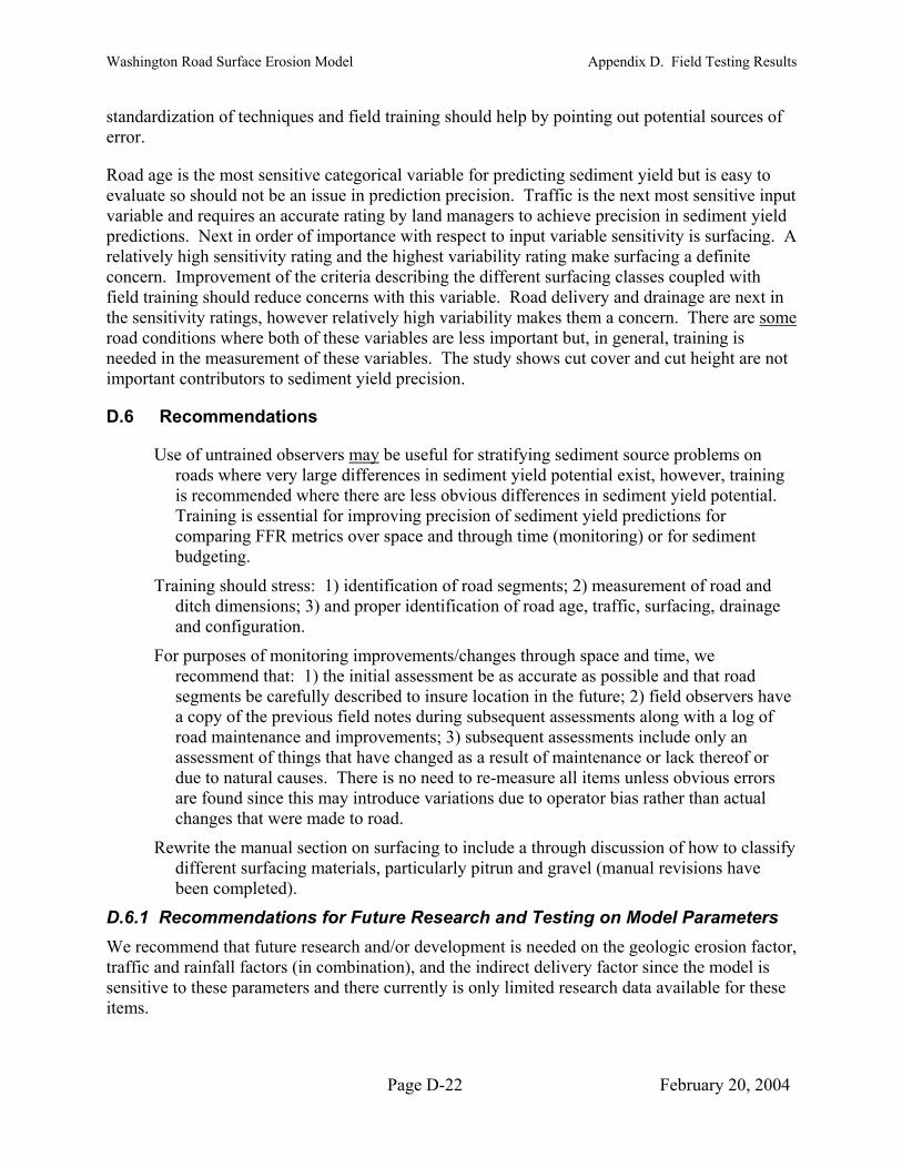
Washington Road Surface Erosion Model Appendix D. Field Testing Results
standardization of techniques and field training should help by pointing out potential sources error.
Road age is the most sensitive categorical variable for predicting sediment yield but is easy toevaluate so should not be an issue in prediction precision. Traffic is the next most sensitive invariable and requires an accurate rating by land managers to achieve precision in sediment
of
put
yield g. A
predictions. Next in order of importance with respect to input variable sensitivity is surfacinrelatively high sensitivity rating and the highest variability rating make surfacing a definite concern. Improvement of the criteria describing the different surfacing classes coupled withfield training should reduce concerns with this variable. Road delivery and drainage are next in the sensitivity ratings, however relatively high variability makes them a concern. There are some road conditions where both of these variables are less important but, in general, training is needed in the measurement of these variables. The study shows cut cover and cut height aimportant contributors to sediment yield
re not precision.
D.6 Recommendations
Use of untrained observers may be useful for stratifying sediment source problems oroads where very large differences in sediment yield potential exist, however, tris recommended where there are less obvious differences in sediment yield potential. Training is essential for improving precision of sediment yield predictions for comparing FFR metrics over space and through time (monitoring) or for sedimentbudgeting.
Training should stress: 1) identification of road segments; 2) measurement of road aditch dimensions; 3) and proper identification of road age, traffic, surfacing, and configuration.
n aining
nd drainage
For purposes of monitoring improvements/changes through space and time, we
e log of
or
D.6.1 Recommendations for Future Research and Testing on Model Parameters
s
recommend that: 1) the initial assessment be as accurate as possible and that road segments be carefully described to insure location in the future; 2) field observers hava copy of the previous field notes during subsequent assessments along with aroad maintenance and improvements; 3) subsequent assessments include only an assessment of things that have changed as a result of maintenance or lack thereofdue to natural causes. There is no need to re-measure all items unless obvious errorsare found since this may introduce variations due to operator bias rather than actual changes that were made to road.
Rewrite the manual section on surfacing to include a through discussion of how to classify different surfacing materials, particularly pitrun and gravel (manual revisions have been completed).
We recommend that future research and/or development is needed on the geologic erosion factor, traffic and rainfall factors (in combination), and the indirect delivery factor since the model isensitive to these parameters and there currently is only limited research data available for theseitems.
Page D-22 February 20, 2004

Washington Road Surface Erosion Model Appendix D. Field Testing Results
In addition, further testing of variability between observers at one or two sites with a wider variation in site conditions and with trained vs. untrained observers would provide better information on how consistent the manual explanations are under these conditions.
One challenge with road erosion research is that there can be very large variations in erosion rates due to variables that are not readily controllable. Rainfall including amount, intensity, antiming is particularly problematic. As a result, even if test sites are carefully planned and controlled, several years of data are needed to get a true idea of how much variability is the result of “natural” variations and how much is the result of differences in the factors you are trying to test. Megahan et al. (1991) show that the erodibility index as defined in the Universal Soil Loss Equation provides a good measure of time integrated rainfall effects on road erosion. Incorporation of recording raingages at road erosion measurement sites would make it possible to adjust for differences in rainfall effects over time and space. Such data also make it possibleto predict long term erosion rates based on the statistical characteristics of rainfall in the general region.
In terms of measurement techniques, only a few sites are monitored in each
d
particular study since accurate measurement of road surface erosion is time-consuming and expensive. The limited
t even more difficult to differentiate between natural variability and differences caused by management changes.
gy t a
ent
ome
ehind the fence.
number of sites makes i
Two different strategies could be employed to overcome these challenges. One potential stratewould be to use a more cost-effective, but lower precision measurement technique, and colleclarger number of samples. This strategy would be useful to test the relative differences in erosion between sites. Traditional road erosion measurements use a large sediment collection chamber to capture the coarse fraction of sediment coupled with a suspended sediment sampling technique to measure the fine-grained fraction of sediment that is contained in overflow water. These sampling techniques are time- and labor-intensive and require the use of heavy equipmto install sampling devices. Robichaud and Brown (2002) discuss a relatively simple erosion sampling method using silt fences. Material collected behind the silt fence is scraped up and weighed by hand in the field. This type of technique is fairly quick and easy to install and measure and requires only hand labor. It is likely that in areas of very fine-grained soils, ssediment would be lost if it was smaller than the silt fence opening size, but this could be accounted for by comparing grain size analysis of road material and material collected b
The other strategy would be to work collaboratively with other road erosion researchers to investigate the potential for joint funding of future projects. There are several researchers actively involved in collecting road erosion measurements across the United States who would likely be interested in collaborative projects.
Geologic Erosion Factor
The present geologic erosion factor was derived by back-calculating the factor at sites where erosion measurements have been made, and the road conditions were known such that appropriate traffic, age, gradient, surfacing, etc. factors could be assigned. There have beestudies that have tested specifically for differences in the inherent erodibility of forest road
n few
segments with all other variables held constant. These types of studies are very difficult to set
ed) suggests that inherent erodibility is strongly up, because it is not possible to hold climate (rainfall) constant between sites. However, recent work by Foltz and Megahan (unpublish
Page D-23 February 20, 2004

Washington Road Surface Erosion Model Appendix D. Field Testing Results
correlated with the percent silt and clay (percent passing the #40 sieve) surface material of the particular road segment. An effective way to test for differences in geologic erosion rates would be to select road sites in fairly close proximity to each other with fairly low traffic use (so that climatic and traffic differences would be minimized) but underlain by different rock types.
Traffic and Rainfall Factors
The traffic and rainfall factors in the current model are treated separately. However, it is most likely that it is the combination of traffic and rainfall together that cause the highest erosion rates. Therefore, the timing of traffic and rainfall, as well as rainfall intensity are important tomeasure together. This requires a more intensive field study procedure that includes collection of traffic counts, rainfall, and erosion using methods that determine the timing of each attrib
ute. It would require installation of traffic counters (that collect traffic and timing information), tipping bucket rainfall gages with data loggers, and collection of erosion data following each storm event or more simply integrated over time.
Indirect Delivery Factor
The distance sediment travels across buffer strips and through vegetated hillslopes has been studieduncertain to determ because t lows. This requ(research ), which is difficult; use of tracer particles (marked silt/clay grains); or a series away fromconsumin
Additi
at several sites. Relationships for sandy soils are fairly well established. However, ty still exists about how far fine-grained sediments (silt, clay) travel. It is more difficultine travel distances for fine-grained sediment since the sediment trail is harder to detecthe finer sediments tend to remain in suspension and move wherever the water fires a study design that either tracks water and sediment movement during storms er observations
of sampling devices, such as turbidity measurement sites, installed at various distances culvert outfalls. Each of these designs has pitfalls and would be fairly time
g but necessary.
onal Variability Testing
similar to those used in the present field test could be used to test the variability rained field observers using the WARSEM model. This would be important for ting model variability for use as a monitoring tool. A test procedure could entail havin observers record road characteristics at several sites, training the observers, and thing data at the same sites to see if observations improved. Alternatively, using two testers, one trained group and one un-trained group at the same site could be used to the effects of training.
dditional sensitivity analysis on a la
Methods between tdocumen g untrained en re-collectgroups ofdetermine
Finally, a rger number of sites would be useful to evaluate differeindividua
D.7 References
Megahan, W.F., S.B. Monsen, M.D. Wilson. 1991. Probability of sediment yields from surface erosion on granitic roadfills in Idaho. Jour. of Environmental Quality, 20 (1): 53-60.
nces by site conditions. This latter could be done with the existing data set using l road segments rather than general site averages as was done for the current test.
Dragovich, J.D., R.L. Logan, H.W. Schasse, T.J. Walsh, W.S. Lingley Jr., D.K Norman, W.J. Gerstel, T.J. Lapen, J.E. Schuster, and K.D. Meyers, 2002. Geologic map of Washington – Northwest quadrant. Washington Division of Geology and Earth Resources Geologic Map GM-50.
Page D-24 February 20, 2004

Washington Road Surface Erosion Model Appendix D. Field Testing Results
Robichaud, P.R., and R.E. Brown, 2002. Silt fences: an economical technique for measuringhillslope soil erosion. Gen. Tech. Rep. RMRS-GTR-94. Fort Collins, CO: U.S. Department of Agriculture, Forest Service, Rocky Mountain Research Station
. 24 p. available on the web at http://www.fs.fed.us/rm/pubs/rmrs_gtr94.pdf.
Tysdal, L.M., W.J. Elliot, C.H. Luce, T.A. Black. 1999. Modeling erosion from insloping low-volume roads with WEPP Watershed Model. In: Seventh international conference on low-volume roads, May 23-26, Baton Rouge, LA, 1999, Transportation Research Record No. 1652, Vol. 2, p. 250-256. National Academy Press, Wash. D.C., 1999.
Walsh, T.J., M.A Korosec, W.M. Phillips, R.L. Logan, and H.W. Schasse, 1987. Geolof Washington – Southwest quadrant. Washington Division of Geology and Earth Resources Geologic Map GM-34.
ogic map
Page D-25 February 20, 2004

Washington Road Surface Erosion Model Appendix D. Field Testing Results
25Maximum
Figure D-1. Mean and range of segment counts by road section
30Mean
10
15
20
Num
ber o
f seg
men
ts
Minimum
0
5
Forks5060
Forks5050
Forks5000
Thrash2100
Thrash2000
Stossel1000
Stossel2000
Road Section
Figure D-2. Length of road assigned to sediment delivery classes by bservers at the Thrash Creek site
DT JC KD KS BM DM DT JC KD KS
o
1500
2000
Leng
th (f
2500
3000
3500
4000
t)
2000 Road 2100 Road
1000
0
500
BM DM
ObserverNo Delivery w/in 200 feet w/in 100 feet Direct Delivery Blank
Page D-26 February 20, 2004

Washington Road Surface Erosion Model Appendix D. Field Testing Results
Figure D-3. Length of road assigned to sediment delivery classes by observers at the Stossel Creek site
0100020003000
A BB BL DL DT LR MMRCD TZ
WM, KD A BL DL DT LR MM
RCD TZ
WM, KD
Observer
Leng
th (f
t)
No Delivery w/in 200 feet w/in 100 feet Direct Delivery Blank
700080009000
10000 1000 Road 2000 Road
400050006000
Page D-27 February 20, 2004
Figure D-4. Length of road assigned to sediment delivery classes by observers at the Forks site
0
1000
2000
3000
4000
5000
6000
DC DO HE JC JD KD TD DC DO HE JC JD KD TD DC DO HE JC JD KD TD
Observer
Leng
th (f
t)
No Delivery w/in 200 feet w/in 100 feet Direct Delivery
5000 Road 5060 Road5050 Road
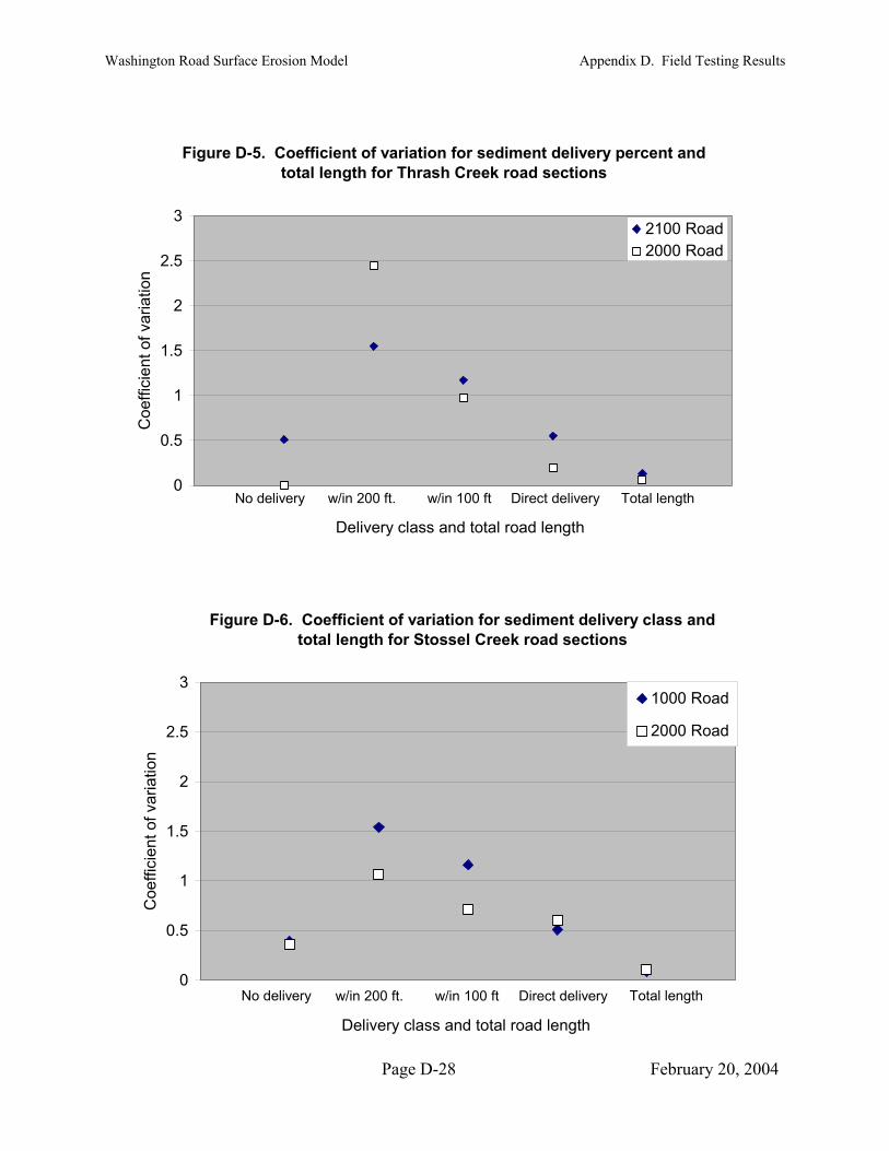
Washington Road Surface Erosion Model Appendix D. Field Testing Results
Figure D-5. Coefficient of variation for sediment delivery percent and total length for Thrash Creek road sections
0
0.5
1
1.5
2
2.5
3
Delivery class and total road length
Coe
ffici
ent o
f var
iatio
n
2100 Road2000 Road
No delivery w/in 200 ft. w/in 100 ft Direct delivery Total length
Figure D-6. Coefficient of variation for sediment delivery class and total length for Stossel Creek road sections
0
0.5
1
1.5
2
2.5
3
Delivery class and total road length
Coe
ffici
ent o
f var
iatio
n
1000 Road
2000 Road
No delivery w/in 200 ft. w/in 100 ft Direct delivery Total length
Page D-28 February 20, 2004

Washington Road Surface Erosion Model Appendix D. Field Testing Results
Figure D-7. Coefficient of variation for sediment delivery percent and total length for Forks road sections
0
0.5
1
1.5
2
2.5
3
Delivery class and total road length
Coe
ffici
ent o
f var
iatio
n
5000 Road5050 Road5060 Road
No delivery w/in 200 ft. w/in 100 ft Direct delivery Total length
Figure D-8. Predicted sediment yields by road and observer Thrash Creek site
0
50
100
150
200
250
300
KD DT BM KS JC DM
Observer
Pre
dict
ed s
edim
ent y
ield
(t/y
r)
2000 Road2100 Road
Page D-29 February 20, 2004
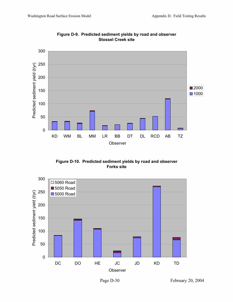
Washington Road Surface Erosion Model Appendix D. Field Testing Results
Figure D-9. Predicted sediment yields by road and observer Stossel Creek site
0
50
100
150
200
250
300
KD WM BL MM LR BB DT DL RCD AB TZ
Observer
Pre
dict
ed s
edim
ent y
ield
(t/y
r)
20001000
Figure D-10. Predicted sediment yields by road and observer Forks site
0
50
100
150
200
250
300
DC DO HE JC JD KD TD
Observer
Pre
dict
ed s
edim
ent y
ield
(t/y
r)
5060 Road5050 Road5000 Road
Page D-30 February 20, 2004

Washington Road Surface Erosion Model Appendix D. Field Testing Results
Figure D-11. Standard deviation vs. mean of predicted sediment yield (t/yr) for individual road segments at the Thrash Creek site
0
0.5
1
1.5
2
2.5
0 0.5 1 1.5 2Mean
Sta
ndar
d de
viat
ion
2100 Road2000 Road
Figure D-12. Standard deviation vs. mean of predicted sediment yield (t/yr) for individual road segments at the Stossel Creek site
0
5
10
15
20
25
0 10 20 30 40 50Mean
Sta
ndar
d de
viat
ion
1000 Road2000 Road
Page D-31 February 20, 2004
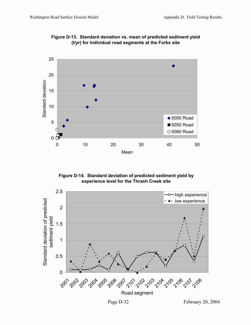
Washington Road Surface Erosion Model Appendix D. Field Testing Results
Figure D-13. Standard deviation vs. mean of predicted sediment yield (t/yr) for individual road segments at the Forks site
0
5
10
15
20
25
0 10 20 30 40 50
Mean
Sta
ndar
d de
viat
ion
5000 Road5050 Road5060 Road
Figure D-14. Standard deviation of predicted sediment yield by experience level for the Thrash Creek site
0
0.5
1
1.5
2
2.5
2001
2002
2003
2004
2005
2006
2007
2101
2102
2103
2104
2105
2106
2107
2108
Road segment
Sta
ndar
d de
viat
ion
of p
redi
cted
se
dim
ent y
ield
high experiencelow experience
Page D-32 February 20, 2004

Washington Road Surface Erosion Model Appendix D. Field Testing Results
Figure D-15. Variability in Length by segment and road Thrash Creek site
0
0.5
1
1.5
2
2.5
3
2101
2102
2103
2104
2105
2106
2107
2108
2001
2002
2003
2004
2005
2006
2007
Road segment and road
Coe
ffici
ent o
f var
iatio
n
Segment averageRoad average
Figure D-16. Variability in Length by segment and road Forks site
0
0.5
1
1.5
2
2.5
3
5001
5002
5003
5004
5005
5006
5007
5008
5051
5052
5053
5054
5055
5056
5057
5058
5059
5061
5062
5063
5064
5065
Road segment and road
Coe
ffici
ent o
f var
iatio
n
Segment averageRoad average
Page D-33 February 20, 2004

Washington Road Surface Erosion Model Appendix D. Field Testing Results
Figure D-17. Variability in Tread Width by segment and road Thrash Creek site
0
0.5
1
1.5
2
2.5
3
2101
2102
2103
2104
2105
2106
2107
2108
2001
2002
2003
2004
2005
2006
2007
Road segment and road
Coe
ffici
ent o
f var
iatio
n
Segment averageRoad average
Figure D-18. Variability in Tread Width by segment and road Stossel Creek data
0
0.5
1
1.5
2
2.5
3
1002
1004
1005
1006
1007
1008
1009
1011
1012
1014
1015
1016
1017
2001
2002
2003
2004
2005
2006
2007
2008
2009
2010
2011
Road segment and road
Coe
ffici
ent o
f var
iatio
n
Segment averageRoad average
Page D-34 February 20, 2004

Washington Road Surface Erosion Model Appendix D. Field Testing Results
Figure D-19. Variability in Tread Width by segment and roadForks site
0
0.5
1
1.5
2
2.5
3
5001
5002
5003
5004
5005
5006
5007
5008
5051
5052
5053
5054
5055
5056
5057
5058
5059
5061
5062
5063
5064
5065
Road segment and Road
Coe
ffici
ent o
f var
iatio
n
Segment averageRoad average
Figure D-20. Variability in Ditch Width by segment and road Thrash Creek site
0
0.5
1
1.5
2
2.5
3
2101
2102
2103
2104
2105
2106
2107
2108
2001
2002
2003
2004
2005
2006
2007
Road segment and road
Coe
ffici
ent o
f var
iatio
n
Segment averageRoad average
Page D-35 February 20, 2004
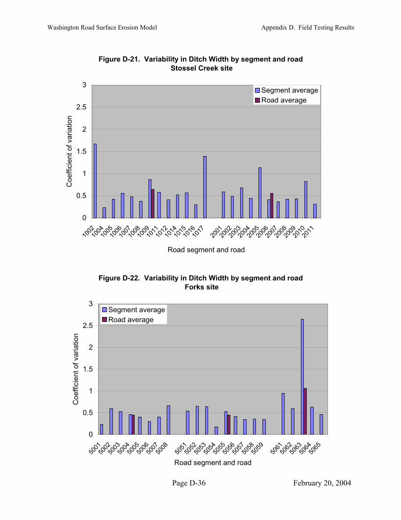
Washington Road Surface Erosion Model Appendix D. Field Testing Results
Figure D-21. Variability in Ditch Width by segment and road Stossel Creek site
0
0.5
1
1.5
2
2.5
3
1002
1004
1005
1006
1007
1008
1009
1011
1012
1014
1015
1016
1017
2001
2002
2003
2004
2005
2006
2007
2008
2009
2010
2011
Road segment and road
Coe
ffici
ent o
f var
iatio
n
Segment averageRoad average
Figure D-22. Variability in Ditch Width by segment and road Forks site
0
0.5
1
1.5
2
2.5
3
5001
5002
5003
5004
5005
5006
5007
5008
5051
5052
5053
5054
5055
5056
5057
5058
5059
5061
5062
5063
5064
5065
Road segment and road
Coe
ffici
ent o
f var
iatio
n
Segment averageRoad average
Page D-36 February 20, 2004
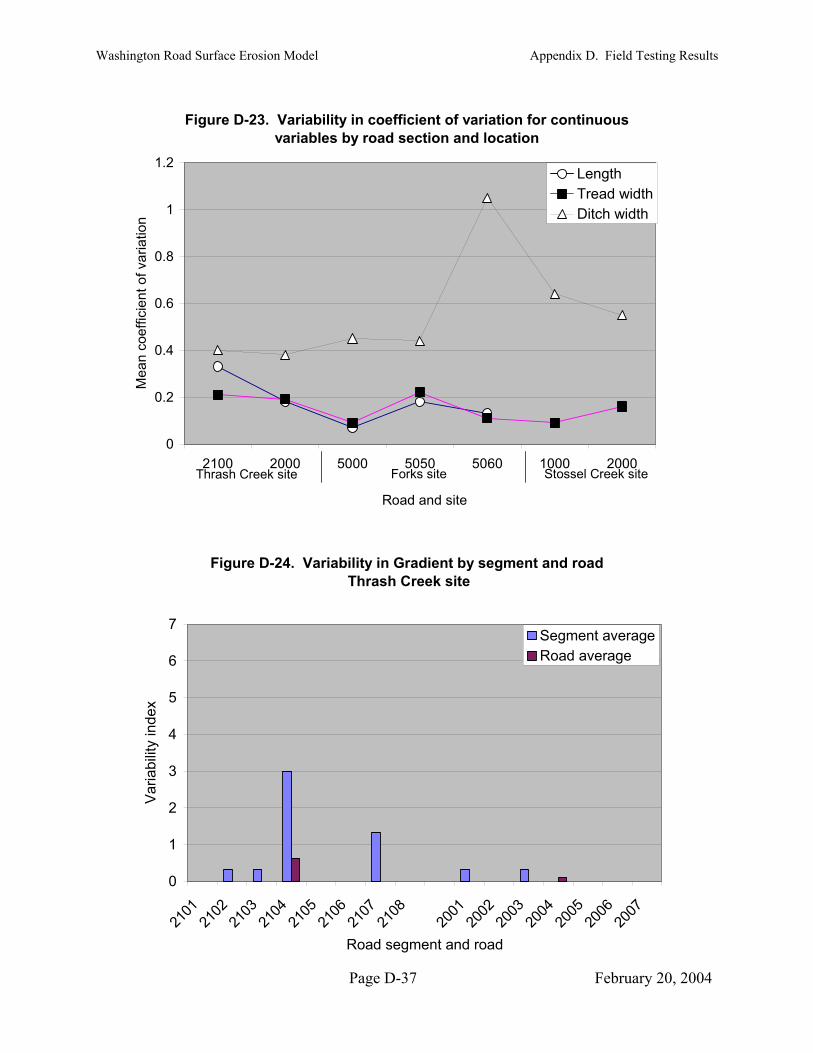
Washington Road Surface Erosion Model Appendix D. Field Testing Results
Figure D-23. Variability in coefficient of variation for continuous variables by road section and location
0
0.2
0.4
0.6
0.8
1
1.2
2100 2000 5000 5050 5060 1000 2000
Road and site
Mea
n co
effic
ient
of v
aria
tion
LengthTread widthDitch width
Thrash Creek site Forks site Stossel Creek site
Figure D-24. Variability in Gradient by segment and road Thrash Creek site
0
1
2
3
4
5
6
7
2101
2102
2103
2104
2105
2106
2107
2108
2001
2002
2003
2004
2005
2006
2007
Road segment and road
Var
iabi
lity
inde
x
Segment averageRoad average
Page D-37 February 20, 2004

Washington Road Surface Erosion Model Appendix D. Field Testing Results
Figure D-25. Variability in Road Gradient by segment and roadStossel Creek site
0
1
2
3
4
5
6
7
1002
1004
1005
1006
1007
1008
1009
1011
1012
1014
1015
1016
1017
2001
2002
2003
2004
2005
2006
2007
2008
2009
2010
2011
Road segment and road
Var
iabi
lity
inde
x
Segment averageRoad average
Figure D-26. Variability in Road Gradient by road segment and roadForks site
0
1
2
3
4
5
6
7
5001
5002
5003
5004
5005
5006
5007
5008
5051
5052
5053
5054
5055
5056
5057
5058
5059
5061
5062
5063
5064
5065
Road segment and road
Var
iabi
lity
inde
x
Segment averageRoad average
Page D-38 February 20, 2004
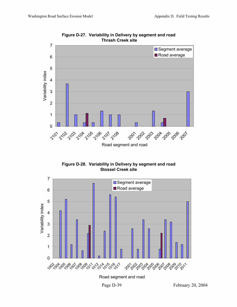
Washington Road Surface Erosion Model Appendix D. Field Testing Results
Figure D-27. Variability in Delivery by segment and road Thrash Creek site
0
1
2
3
4
5
6
7
2101
2102
2103
2104
2105
2106
2107
2108
2001
2002
2003
2004
2005
2006
2007
Road segment and road
Var
iabi
lity
inde
xSegment averageRoad average
Figure D-28. Variability in Delivery by segment and road Stossel Creek site
0
1
2
3
4
5
6
7
1002
1004
1005
1006
1007
1008
1009
1011
1012
1014
1015
1016
1017
2001
2002
2003
2004
2005
2006
2007
2008
2009
2010
2011
Road segment and road
Var
iabi
lity
inde
x
Segment averageRoad average
Page D-39 February 20, 2004
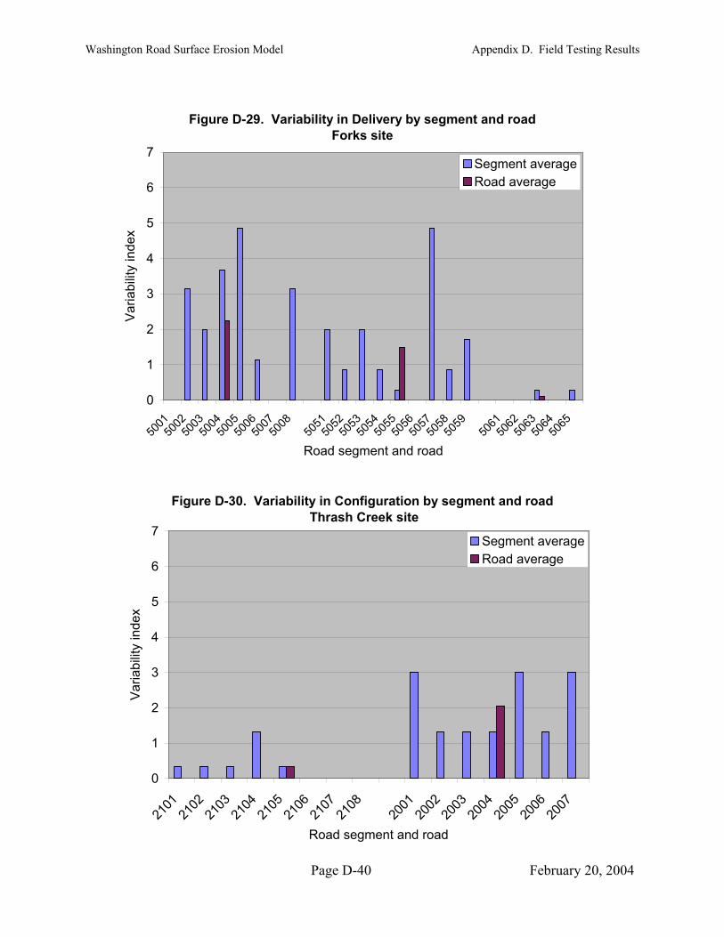
Washington Road Surface Erosion Model Appendix D. Field Testing Results
Figure D-29. Variability in Delivery by segment and roadForks site
0
1
2
3
4
5
6
7
5001
5002
5003
5004
5005
5006
5007
5008
5051
5052
5053
5054
5055
5056
5057
5058
5059
5061
5062
5063
5064
5065
Road segment and road
Var
iabi
lity
inde
x
Segment averageRoad average
Figure D-30. Variability in Configuration by segment and road Thrash Creek site
0
1
2
3
4
5
6
7
2101
2102
2103
2104
2105
2106
2107
2108
2001
2002
2003
2004
2005
2006
2007
Road segment and road
Var
iabi
lity
inde
x
Segment averageRoad average
Page D-40 February 20, 2004
Washington Road Surface Erosion Model Appendix D. Field Testing Results
Figure D-31. Variability in Configuration by segment and road Stossel Creek site
0
1
2
3
4
5
6
7
1002
1004
1005
1006
1007
1008
1009
1011
1012
1014
1015
1016
1017
2001
2002
2003
2004
2005
2006
2007
2008
2009
2010
2011
Road segment and road
Var
iabi
lity
inde
x
Segment averageRoad average
Figure D-32. Variability in Configuration by road segment and road Forks site
0
1
2
3
4
5
6
7
5001
5002
5003
5004
5005
5006
5007
5008
5051
5052
5053
5054
5055
5056
5057
5058
5059
5061
5062
5063
5064
5065
Road segment and road
Var
iabi
lity
inde
x
Segment averageRoad average
Page D-41 February 20, 2004
Washington Road Surface Erosion Model Appendix D. Field Testing Results
Figure D-33. Variability in Surfacing by road segment and road Thrash Creek site
0
1
2
3
4
5
6
7
2101
2102
2103
2104
2105
2106
2107
2108
2001
2002
2003
2004
2005
2006
2007
Road segment and road
Var
iabi
lity
inde
x
Segment averageRoad average
Figure D-34. Variability in Surfacing by segment and road Stossel Creek site
0
1
2
3
4
5
6
7
1002
1004
1005
1006
1007
1008
1009
1011
1012
1014
1015
1016
1017
2001
2002
2003
2004
2005
2006
2007
2008
2009
2010
2011
Road segment and road
Var
iabi
lity
inde
x
Segment averageRoad average
Page D-42 February 20, 2004

Washington Road Surface Erosion Model Appendix D. Field Testing Results
Figure D-35. Variability in Surfacing by segment and road Forks site
0
1
2
3
4
5
6
7
5001
5002
5003
5004
5005
5006
5007
5008
5051
5052
5053
5054
5055
5056
5057
5058
5059
5061
5062
5063
5064
5065
Road segment and road
Var
iabi
lity
inde
x
Segment averageRoad average
Figure D-36. Variation in Cut Cover by segment and road Thrash Creek site
0
1
2
3
4
5
6
7
2101
2102
2103
2104
2105
2106
2107
2108
2001
2002
2003
2004
2005
2006
2007
Road segment and road
Var
iabi
lity
inde
x
Segment averageRoad average
Page D-43 February 20, 2004

Washington Road Surface Erosion Model Appendix D. Field Testing Results
Figure D-37. Variability in Cut Cover by segment and road Stossel Creek site
0
0.5
1
1.5
2
2.5
3
3.5
4
4.5
5
1002
1004
1005
1006
1007
1008
1009
1011
1012
1014
1015
1016
1017
2001
2002
2003
2004
2005
2006
2007
2008
2009
2010
2011
Road segment and road
Var
iabi
lity
inde
x
Segment averageRoad average
Figure D-38. Variability in Cut Cover by road segment and road Forks site
0
1
2
3
4
5
6
7
5001
5002
5003
5004
5005
5006
5007
5008
5051
5052
5053
5054
5055
5056
5057
5058
5059
5061
5062
5063
5064
5065
Road segment and road
Var
iabi
lity
inde
x
Segment averageRoad average
Page D-44 February 20, 2004
Washington Road Surface Erosion Model Appendix D. Field Testing Results
Figure D-39. Variability in Cut Height by segment and road Thrash Creek site
0.0
1.0
2.0
3.0
4.0
5.0
6.0
7.0
2101
2102
2103
2104
2105
2106
2107
2108
2001
2002
2003
2004
2005
2006
2007
Road segment and road
Var
iabi
lity
inde
x
Segment averageRoad average
Figure D-40. Variability in Cutslope Height by segment and road Stossel Creek site
0
1
2
3
4
5
6
7
1002
1004
1005
1006
1007
1008
1009
1011
1012
1014
1015
1016
1017
2001
2002
2003
2004
2005
2006
2007
2008
2009
2010
2011
Road segment and road
Coe
ffici
ent o
f var
iatio
n
Segment averageRoad average
Page D-45 February 20, 2004

Washington Road Surface Erosion Model Appendix D. Field Testing Results
Figure D-41. Variability in Cut Height by road segment and road Forks site
0.0
1.0
2.0
3.0
4.0
5.0
6.0
7.0
5001
5002
5003
5004
5005
5006
5007
5008
5051
5052
5053
5054
5055
5056
5057
5058
5059
5061
5062
5063
5064
5065
Road segment and road
Var
iabi
lity
inde
x
Segment averageRoad average
Figure D-42. Variability of road properties Thrash Creek site (class variables)
0
0.5
1
1.5
2
2.5
3
3.5
Var
iabi
lity
inde
x
Primary roadSpur roadOverall Mean
Gradient DeliveryConfig. SurfacingCut cover Cut height
Page D-46 February 20, 2004
Washington Road Surface Erosion Model Appendix D. Field Testing Results
Figure D-43. Variability of road properties at Stossel Creek site (class variables)
0
0.5
1
1.5
2
2.5
3
3.5
Var
iabi
lity
inde
x
Mainline
Gated spurroadMean
Gradient DeliveryConfig. SurfacingCut cover Cut height
Figure D-44. Variability of road properties at Forks site (class variables)
0
0.5
1
1.5
2
2.5
3
3.5
Gradient Cut cover Config. Delivery Cut height Surfacing
Var
iabi
lity
inde
x
5000 road5050 road5060 roadmean
Page D-47 February 20, 2004
Washington Road Surface Erosion Model Appendix D. Field Testing Results
Figure D-45. Overall average values and statistical differences of VI for categorical input variables
0.0
0.5
1.0
1.5
2.0
2.5
Gradient Cut cover Config. Delivery Cutheight
Surfacing
Categorical variable
Mea
n va
riabi
lity
inde
x
Note -- Presence of a horizontal bar below a set of variables indicates there are no statistical differences between the variables over the bar but there are statistical differences (P =0.1) between any of the variables over the bar and all other variables not over the bar.
Figure D-46. Sensitivity analysis of WARSEM variables Thrash Creek site
0
10
20
30
40
50
60
70
80
Road A
geTraf
fic
Precipi
tation
Surfac
ing
Geolog
y
Road G
radien
t
Total D
elive
ry
Config
uratio
n
Cut Cov
er
Cut Heig
ht
Variable
Ran
ge in
sed
imen
t yie
ld t/
yr
Range Total Sediment
Page D-48 February 20, 2004

Washington Road Surface Erosion Model Appendix D. Field Testing Results
Figure D-47. Sensitivity analysis of WARSEM variables Stossel Creek site
0
10
20
30
40
50
60
70
80
Road A
geTraf
fic
Precipi
tation
Surfac
ing
Geolog
y
Road G
radien
t
Total D
elive
ry
Config
uratio
n
Cut Cov
er
Cut Heig
ht
Variable
Ran
ge in
sed
imen
t yie
ld (t
/yr) Range Total Sediment
Figure D-48. Sensitivity analysis of WARSEM variablesForks site
0
10
20
30
40
50
60
70
80
Road A
geTraf
fic
Precipi
tation
Surfac
ing
Geolog
y
Road G
radien
t
Total D
elive
ry
Config
uratio
n
Cut Cov
er
Cut he
ight
Variable
Ran
ge in
sed
imen
t yie
ld (t
/yr) Range Total Sediment
Page D-49 February 20, 2004
Washington Road Surface Erosion Model Appendix D. Field Testing Results
Figure D-49. Average sensitivity ranking of WARSEM variables for all sites
0123456789
10
Road A
geTraf
fic
Precipi
tation
Surfac
ing
Geolog
y
Road G
radien
t
Total D
elive
ry
Config
uratio
n
Cut Cov
er
Cut Heig
ht
Variable
Ave
rage
sen
sitiv
ity ra
nk
Page D-50 February 20, 2004

Appendix E. Data Import Format Requirements


Washington Road Surface Erosion Model Appendix E. Data Import Format Requirements
Appendix E. Data Import Format Requirements
The following table shows the required order and content of data fields for any files that will be used to import data into the WARSEM application. It is not required that all fields be present in the import records, but shaded fields are required. The content of data fields must conform to that noted in the table, with spelling, case, and values as noted.
SEDMODL2 Special Instructions
Although WARSEM supports importing SEDMODL2 model output files into a project, a significant amount of additional work is required after the import to complete translating the SEDMODL2 file. The additional work includes assigning:
• Township, Range, and Section
• Project Area number
• Field
An alternative is to complete additional GIS processing to by overlaying a Township coverage onto the roads, assigning the majority length to one Section within a Township. Additional GIS processing can assign an appropriate Project Area and Field Verification status. Once these processes are complete, the attribute data can be exported to a dBase file or Excel file and imported. This approach would also require translating Road Gradient and Cutslope Cover values into the WARSEM classes (see documentation). GIS road data using meters as the unit of measure will need to be converted to feet for road segment length. Please carefully review your data for completeness and accuracy before attempting an import into WARSEM.
verification status
Page E-1 February 20, 2004

rosi
on M
odel
A
ppen
dix
E. D
ata
Impo
rt Fo
rmat
Req
uire
men
ts
Page
E-2
Fe
brua
ry 2
0, 2
004
App
endi
x E.
Dat
a Im
port
For
mat
Req
uire
men
ts
Dat
a T
ype
Max
L
engt
h D
escr
iptio
n an
d fo
rmat
req
uire
men
ts
Long
inte
ger
U
niqu
e Id
entif
ier f
or ro
ad se
gmen
t. D
uplic
ates
not
allo
wed
Was
hing
ton
Roa
d Su
rfac
e E
Fiel
d N
ame
Seg_
ID
Gro
up_I
D
Roa
dNam
e Pr
ojec
tAre
a Pr
imTw
p Pr
imR
ng
Prim
Sec
Leng
th
Flag
R
dCla
ss
RdS
urf
Trea
dWid
th
Ditc
hWid
th
Ditc
hDel
Type
In
tD
itchC
ond
RdU
se
Text
RdG
radi
ent
Rdc
utsl
pht
Cut
slpv
eg
Rdp
rism
C
onst
ruct
yr
Geo
logy
Del
code
In
Fiel
dVer
ified
= R
equi
red
Long
inte
ger
ID
num
ber f
or c
ontig
uous
road
segm
ents
with
shar
ed d
eliv
ery
rout
e (e
xten
ded
drai
nage
net
wor
k)
Text
30
U
ser d
efin
ed ro
ad n
ame
Text
Uni
que
iden
tifie
r for
iden
tifyi
ng th
e lo
catio
n of
the
road
segm
ent w
ithin
a W
AU
Te
xt
4 To
wns
hip
whe
re th
e m
ajor
ity o
f the
road
exi
sts,
(Val
id F
orm
at: T
00N
) Te
xt
4 R
ange
whe
re th
e m
ajor
ity o
f the
road
exi
sts,
(Val
id F
orm
at: R
00E,
or R
00W
) In
tege
r
Sect
ion
num
ber w
here
the
maj
ority
of a
road
exi
sts.
(1-3
6)
Sing
le
Le
ngth
of r
oad
segm
ent i
n fe
et.
Inte
ger
In
dica
tor f
or a
pplic
atio
n of
upd
ates
or a
ctio
ns w
here
Fla
g >
0.
Text
17
H
ighw
ay, M
ain
haul
, Cou
nty
road
, Prim
ary
road
, Sec
onda
ry ro
ad, S
pur r
oad,
Aba
ndon
ed/b
lock
ed
Text
17
A
spha
lt, G
rave
l, G
rave
l with
ruts
, Pit
run,
Gra
ssed
nat
ive,
Nat
ive,
Nat
ive
with
ruts
In
tege
r
Wid
th o
f roa
d tre
ad in
feet
. In
tege
r
Wid
th o
f ditc
h in
feet
.
eger
Del
iver
y ty
pe c
ode
for d
itch
(Val
id C
odes
: 0 =
No
deliv
ery;
1=D
irect
; 2=I
ndire
ct<=
100
Ft.;
3=In
dire
ct 1
01-2
00 F
t; 4=
Dire
ct v
ia g
ully
.) Te
xt
8 C
ondi
tion
of d
itch
(Val
id C
lass
es: R
OC
K/V
EG, S
TAB
LE, E
RO
DIN
G)
16
Ty
pica
l roa
d us
e: (V
alid
Cla
sses
: NO
NE,
OC
CA
SIO
NA
L, L
IGH
T, M
OD
ERA
TE, M
OD
ERA
TELY
HEA
VY
, HEA
VY
) In
tege
r
Act
ual v
alue
s can
be
used
but
the
mod
el c
lass
ifies
the
data
into
(0-5
%, 5
-10%
, > 1
0%).
Mus
t be
who
le n
umbe
r. In
tege
r
Hei
ght o
f cut
slop
e (in
feet
). A
ctua
l val
ues a
ccep
ted
but c
lass
ified
into
: 0 ft
, 2.5
ft, 5
ft, 1
0ft,
25ft
Inte
ger
Pe
rcen
tage
of c
over
of v
eget
ativ
e or
non
-ero
sive
mat
eria
l on
road
cut
slop
e. (
Who
le n
umbe
r, 0-
100)
Te
xt
9 R
oad
conf
igur
atio
n (V
alid
Cla
sses
: Ins
lope
d, O
utsl
oped
, Cro
wne
d)
Inte
ger
Y
ear o
f roa
d co
nstru
ctio
n (V
alid
For
mat
: yyy
y)
Text
8
Des
crip
tion
of g
eolo
gy a
s see
n on
the
cuts
lope
. (V
alid
Cla
sses
: Low
, Med
ium
, Hig
h)
tege
r
Del
iver
y ty
pe c
ode
(Val
id C
odes
: 0 =
No
deliv
ery;
1=D
irect
; 2=I
ndire
ct<=
100
Ft.;
3=In
dire
ct 1
01-2
00 F
t; 4=
Dire
ct v
ia
gully
.) Te
xt
3 H
ave
the
road
attr
ibut
es b
een
field
ver
ified
. (V
alid
Cod
es: Y
ES, N
O)
fiel
d

Washington Road Surface Erosion Model Appendix E. Data Import Format Requirements
Appendix E. (Continued)
Data Preparation and Import Considerations:
• Required fields (shaded and Required in parenthesis) must be present in the import file. Optional fields must be located in a position relative to required fields, and other selected optional fields. The WARSEM Data Import Utility dialog assists the user with identifying
the type of file to import, and the fields present in the import file. Error messages will be generated when required fields are missing or when
ords (road segments) that represent a rticularly helpful for discrete GIS features that are
ents with roves reporting and the ability to recognize significant sediment
diment totals of individual records may be insignificant ollectively as a delivery system.
ch
m definitions do not match the required format.
• Even though WARSEM uses data classes for many of the model parameters it’s possible to import actual values and the application will complete the classification on the fly. This applies to: Road Gradient, Cutslope Height, and Cutslope Cover.
• Comma delimited text files must have text fields formatted with double quotation marks. (Example: Seg_ID, Group_ID, Road Name,… would be 1,1,”Mill Road”)
• It is not required that your field names be consistent with the names listed above. What is important is the order of the fields and their data type definitions.
• If import records are missing values for required fields the application will prompt the user to select a default value that will be used to substitute null values with. This will slow the import process down, users will experience a lower frustration level by carefully examining their data to insure conformance with the application data requirements.
and locating the file to be imported,
record values or field definitions conflict with data requirements.
• Seg_ID and Group_ID can be used together to group reccommon delivery system. This is paseparated due to arc/node topology or differences in attributes. Grouping road segma shared delivery path imptotals. Without grouping, seindividually but significant c
• If Project Area is imported it will be necessary to update the Project Area Builder to assign Management Block, WAU, Miles of Stream, Application Level, and Data Resolution to eaof the project areas imported.
• When an import process has been initiated the user will be asked to indicate which items are present in the file to be imported. Failure to accurately indicate the items present in the import file will result in a failed import. An import failure may also occur if ite
Page E-3 February 20, 2004


![Surface uplift, tectonics, and erosion of eastern Tibet ...kwhipple/papers/Clark_etal_2004_Tectonics.pdf · SURFACE UPLIFT, TECTONICS, AND EROSION OF EASTERN TIBET 2of20 TC1006 [6]](https://img.pdfslide.net/doc/110x75/5f71758689e8c55edf042273/surface-uplift-tectonics-and-erosion-of-eastern-tibet-kwhipplepapersclarketal2004tectonicspdf.jpg)