WASHU-T-74-001 c. 2LOAN CGPV OSI-~

CIRCUI ATlNG COPY

Sea Grant Depositor',

A HYDROACOUSTIC DATA ACQUISITIONAND DIGITAL DATA ANALYSIS SYSTEM

FOR THE ASSESSMENT

OF FISH STOCK ABUNDANCE

By Edmund Pierce Nunnallee, Jr.

WSG 74-2

Hay 1974

1VI.11 !N MA141NE Hl=.. i !l /R :LS

1 JN1V1'lC. il'['Y !F WA.iHilN i'il' !N ~!Hl~!R

Pr .pared under lhc

NatiOr!al SCa Gr;!nl PrOgram

A RASHINhTON SEA GRANT . UHLICATION

WSG 74-2

A HYDROACOUSTIC DATA ACQUISITIONAND DIGITAL DATA ANALYSIS SYSTEM

FOR THE ASSESSMENTOF FISH STOCK ABUNDANCE

By Edmund Pierce Nunnallee, Jr.

May 1974Published by Division of Marine ResourcesUniversity of Washington Seatt'fe 98195

in cooperation wi th

Fi sheries Research Insti tuteCollege of Fisheries, University of Washington

ABSTRACT

A hydroacoustic data acquisition and digital data analysis system

has been designed and constructed at the University of Washington, Seattle,

to measure the abundance of pelagic fish. The portable data acquisition

unit consists of an echo sounder interfaced to a magnetic tape recorder.

The digital data analysis unit incorporates a small computer, a line

printer, and various hardware to interface the computer to an echo sounder

or a tape player.

Thi 8 paper was written to provide a basic operators manual f or the

hydroacoustic data acquisition and analysis system and to compile various

publications relative to its use. General descriptions, instructions for

use, and theory of operation are given for each ma]or component of the

system. Several methods for the analysis of recorded hydroacoustic data

are also included.

ACKNOWLEDGMENT

The research reported in this publication was supported by the

Washington Sea Grant Program under grant number 04-3-158-42 from the National

Oceanic and Atmospheric Administration, U. S. Department of Commerce.

CONTENTS

LIST OF FIGURES. e . V

INTRODUCTION............ o -............ l

A HYDROACOUSTIC DATA ACQUISITION AND DIGITALDATA ANALYSIS SYSTEM ~ ~ ~ ~ 2

The Hydroacoustic Data Acquisition Unit 5

Descript ion ~ ~ ~ ~ ~ ~ ~ ~ ~ ~ ~ ~ ~ o ~ ~ ~ ~Equipment Setup in the FieldEquipment Operation in the Field

~ ~ ~ ~ 5

e ~ ~ ~ 6

~ ~ ~ ~ 7

The Digital Data Analysis Unit DDAU! . . . . . . . . . . . 17

General Description ~ ~ ~ ~ 17

Detailed Descriptions of the DDAU Componentsand Operations . . . . . . . . , , . . . . . . . . . , . 20

Input Amplifier~ ~

Rectifier

Filtering and Sampling CircuitAnalog-to-Digital ConverterSquaring CircuitIntegrator and Triggering CircuitControl Console, Tape Reader, and

~ ~ ~ ~ ~ ~ 20

~ ~ 4 ~

~ ~ ~ ~

~ ~ ~ ~

~ ~ ~ ~~ ~ ~ ~ 26

~ ~ ~ ~ 27

~ ~Line Printer

METHODS OF DATA ANALYSIS ~ ~ ~ ~ ~ ~ ~ 29

Estimation of Effective Sample Volume bythe Use of an Oscilloscope

Estimation of Fish Density by the Use oFan Oscilloscope

Estimation of Fish Density by Echo Inte-gration 0 t ~ 0 ~ ~ ~ ~ ~ ~ ~ t ~ ~ 4 ~

~ ~ ~ ~ ~ ~ ~ e ~ 30

~ ~ ~ ~ ~ ~ ~ ~ ~ 37

~ ~ ~ ~ ~ ~ ~ 41

LITERATURE CITED ~ ~ ~ 0 46

LIST OF TABLES ~ ~ ~ . . ~ . . . . . . ~ ~ ~ ~ + ~ ~ ~ ~ ~ ~ ~ . iv

LZST OF TABLES

Table Page

l Nominal settings and signal levels of the datacollection system . . . . . . . . . . . . . . . . . . . , . . ll

2 Output fcmnat of the digital dakota analysis unit . . . , . . . 29

LIST OF FIGURES

Figure Page

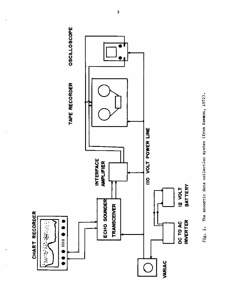
The acoustic data collection system from Dawson, 1972!. ~ ~ ~ ~ 3

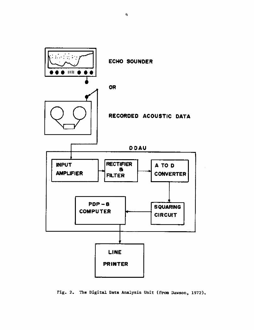
The Digital Data Analysis Unit from Dawson, 1972! ~ ~ ~ ~ 4

Typical test waveforms as viewed on an oscilloscopeat the indicated system tast points ~ ~ ~ ~ 8

Block diagram of the data acquisition unit showingthe various test points ~ ~ ~ ~ 10

The relationship of input and playback signal voltagesof a tape recorder showing the effect of magnetictape saturation ~ ~ ~ ~ 12

Comparison of a 20 Log R curve and a TVG curve asmeasured in an echo sounder 14

A curve showing the effect of the gain controlsetting on receiver sensitivity

Interference on the R channel signal baseline using A! high and B! low L channel record level settingsof a tape recorder . . . . . . . . . , , , . . . . , ~ ~ ~ ~ ~ ~ 18

Block diagram of the digital data analysis unitshowing the locations of the oscilloscipe testpoints ~ ~ ~ ~ ~ ~ ~ e 19

Simulated oscilloscope display showing the waveforms present at test points 1, 2, 3, and 4 inFig. 9 A, B, C, and D!.

10

21

Envelope detection of an echo pulse showing A!conversion of the 5 kHz frequency to B! a DCvoltage pulse and C! the effect of filtering ~ ~ ~ ~ ~ t ~ ~ 23

Input and output wave forms of the samplingcircuit for a 1-ms pulse duration sampled ata rate of 5 kHz �/ms!

12

~ ~ ~ o ~ ~ ~ ~ 24

13

~ ~ ~ e ~ t e ~ 31

directivity~ ~ ~ ~ ~ 34

Illustration of the polar coordinatein the definition of the directivitya transducer .

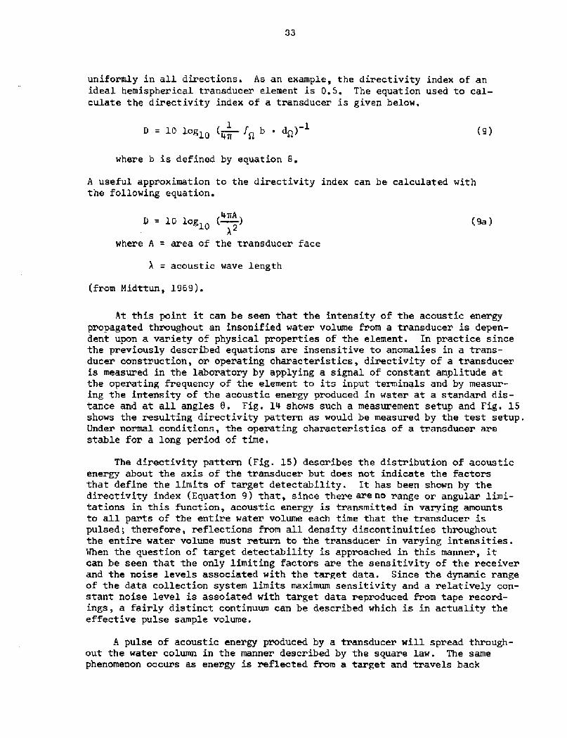
A basic test setup for measuring thecharacteristics of a transducer

system usedfunction of

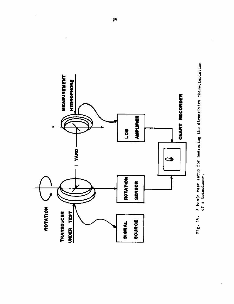
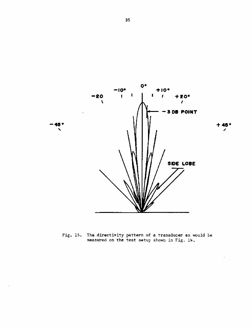
15 The directivity pattern of a transducer as wouldbe measured on the test setup shown in Fig. 14 , 35

16 The relationship of the percentages of total num-bers to the range of observed numbers of insoni-fications/fish over a series of contiguous depthstrata ~ ~ ~ ~ ~ t ~ ~ ~ t ~ ~ ~ ~ ~ ~ ~ ~ ~ ~ ~ ~ ~ ~ ~ o ~ ~ 38

~ ~ ~ ~ ~ ~ 39

17 An illustration of two methods for calculating thevolume of a frustum of a right cone . ~

A HYDROACOUSTIC DATA ACQUISITION AND DIGITAL DATA ANALYSIS SYSTEMFOR THE ASSESSMENT OF FISH STOCK ABUNDANCE

INTRODUCTION

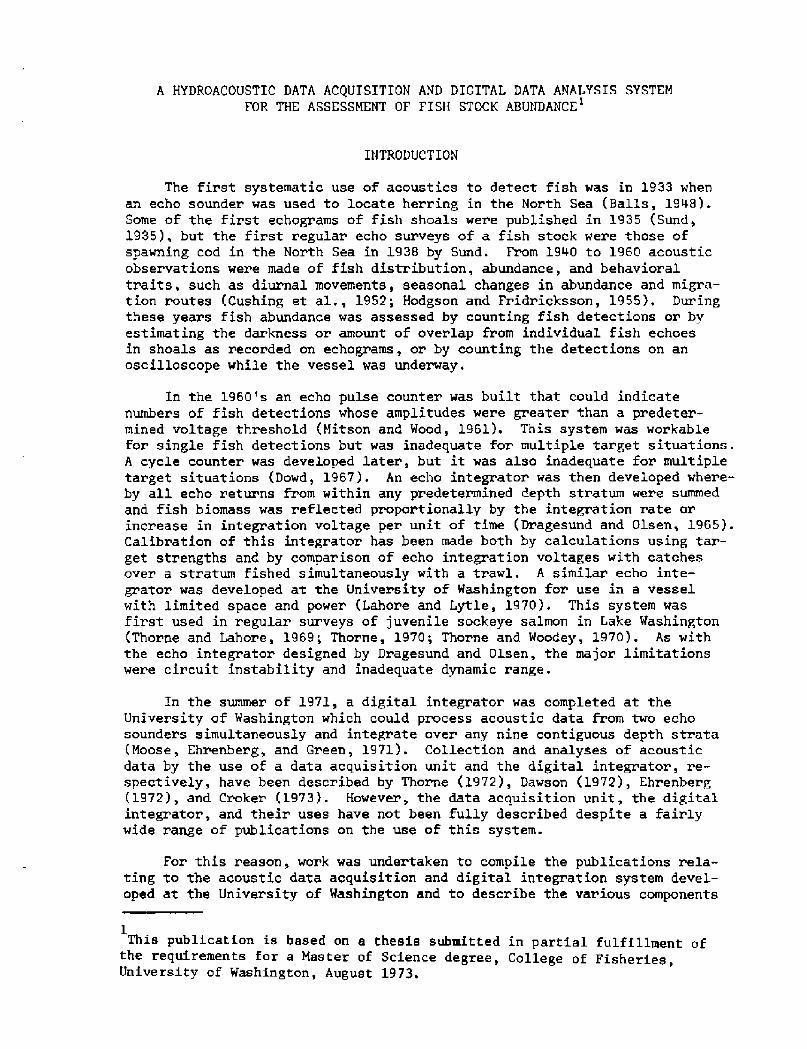
The first systematic use of acoustics to detect fish was in 1933 whenan echo sounder was used to locate herring in the North Sea Balls, 1948!.Some of the first echograms of fish shoals were published in 1935 Sund,1935!, but the first regular echo surveys of a fish stock were those ofspawning cod in the North Sea in 1938 by Sund. From 1940 to 1960 acousticobservations were made of fish distribution, abundance, and behavioraltraits, such as diurnal movements, seasonal changes in abundance and migra-tion routes Cushing et al., 1952; Hadgson and Fridrickssan, 1955!. Duringthese years fish abundance was assessed by counting fish detectians or byestimating the darkness or amount of overlap from individual fish echoesin shoals as recorded an echograms, or by counting the detections on anoscilloscope while the vessel was underway.

In the 1960's an echo pulse counter was built that could indicatenumber's of fish detections whose amplitudes were greater than a predeter-mined voltage threshold Mitson and Wood, 1961!. This system was workablefor single fish detections but was inadequate for multiple target situations.A cycle counter was developed later, but it was alsa inadequate for multipletarget situations Dowd, 1967!. An echo integrator was then developed where-by all echo returns from within any predetermined depth stratum were summedand fish biomass was reflected proportionally by the integration rate orincrease in integration voltage per unit of time Dragesund and Olsen, 1965!.Calibration of this integrator has been made bath by calculations using tar-get strengths and by comparison of echo integration voltages with catchesover a stratum fished simultaneously with a trawl. A similar echo inte-grator was developed at the University of Washington for use in a vesselwith limited space and power Lahare and Lytle, 1970!. This system wasfirst used in regular surveys of juvenile sockeye salmon in Lake Washington Thorne and Lahore, 1969; Thorne, 1970; Thorne and Woodey, 1970!. As withthe echo integrator designed by Dragesund and Olsen, the major limitationswere circuit instability and inadequate dynamic z'ange.

In the summer of 1971, a digital integrator was completed at theUniversity of Washington which could process acoustic data from two echosounders simultaneously and integrate over any nine contiguous depth strata Moose, Ehrenberg, and Green, 1971!. Collection and analyses of acousticdata by the use of a data acquisition unit and the digital integrator, re-spectively, have been described by Thorne �972!, Dawson �972!, Ehrenberg�972!, and Croker �973!. However, the data acquisition unit, the digitalintegrator, and their uses have not been fully described despite a fairlywide range of publications on the use of this system.

Far this reason, work was undertaken to compile the publications rela-ting to the acoustic data acquisition and digital integration system devel-oped at the University of Washington and to describe the various components

IThis publication is based on a thesis submitted in partial fulfillment of

the requirements for a Master of Science degree, College of Fisheries,University of Washington, August 1973.

and their opezation in language understandable to fishery biologists, Inthis paper is presented a users' manual describing the workings of the dataacquisition system, its setup and opezation in the field, the basic componentsof the digital data analysis system and their functions, and its setup priorto data analysis. Also detailed are various techniques for data analysis.

A HYDROACOUSTIC DATA ACQUISITION AND DIGITAL DATA ANALYSIS SYSTEM

Two major units comprise the hydroacoustic data acquisition and proces-sing system. The first consists of an echo sounder and tape recorder inter-faced by a small frequency convez'ter and, is a portable unit used for dataacquisition in the field. The second includes a digitizer, a computer-integrator, a line printer, and associated hardware, and is used for anal-ysis of data collected with the portable unit. The entire system may bemounted aboard ship, but the data analysis unit is basically a laboratoryinstrument. A brief overview of the system, its opezation and use will begiven, followed by detailed descriptions of the basic components of eachunit.

The hydroacoustic data acquisition system is basically a recording echosounder. Target information is stored in two ways, as echograms and on mag-netic recording tape. Echograms are usable only as a gross indication offish density or depth, while analysis of the data recorded on magnetic tapecan yield quantitative information as to fish density, depth, distribution,and size. The data acquisition system is composed of several interconnectedunits including an echosounder equipped with a narrow beam transducer andseparate chart recorder, a small frequency converter and a stereo tape re-coz'der. The units can be powered directly from a 117 VAC source, or by astorage battery and a DC to AC inverter. Figure 1 shows the layout andinterconnections of the various parts of the data collection system.

The data processing unit is basically a digital echo integrator. Theterm echo integrator derives from the fact that the unit sums voltages pro-portional to target echo intensities over any predetermined time-depthinterval. Because echo intensities are directly proportional to the bio-mass of the reflecting targets, the summed voltages z'epz'esent biomassmeasurements. Also, if there is no great amount of variability associatedwith average fish biomass, then numerical estimates are also possible. Asis the case with the data acquisition system, the data analysis system isalso composed of a number of interconnecting units. A detailed descz iptionof the operation and theory of each unit will be given later in the text.The basic configuration of the analysis system is shown in Fig. 2. Notethat the heart of the unit consists of a small general purpose computerthat allows the unit to be used for a vaz'iety of tasks beside echo integra-tion. It is a large, rack-mounted instrument and weighs several hundred

This system has been referred to by other writers as the Digital DataAcquisition and Processing System DDAPS!.

4 0

A

0+I0I4

0

O 0 0 rdO

R O I-Ct

Z O

4 p0 a'

ECHO SOUNOKR

Fig. 2. The Digital Data Analysis Unit from Dawson, 1972!.

pounds including a separate oscilloscope, tape player, and line printer.The unit requix'es several hundred watts of 117 VAC power and therefore isusable only on a fairly large vessel with adequate generators or in thelaboratory.

The H droacoustic Data Ac uisition Unit

The components are a Ross 200A echo soundex, an interface amplifierthat was designed and built at the University of Washington, and a Sony560D stereo tape recorder. The operation is monitored with a small,battery-powered oscilloscope.

The Ross 200A echosounder and chax't recorder are commercially avail-able as standard shelf items. A narrow beam transducer 8~ full angle!is also available from the manufacturex on special order. This unit wasincorporated in the data collection system fox economic reasons xatherthan for quality ox reliabi?ity and should be avoided in future uses be-cause of its archaic design and construction. Three modifications havebeen incorporated in the Ross echo sounder. They are the replacement ofthe single turn gain control potentiometer with a 10 turn Helipot, theaddition of an isolation amplifier to decouple the signal output, and theaddition of a calibration oscillator.

The addition of a l0 turn gain control was not a circuit modifica-tion but was done to allow better mechanical repeatability of gain set-tings. An isolation amplifier was added so that the high impedancevacuum tube circuitry of the echo sounder receiver would be unaffectedby the cabling to other parts of the data acquisition system. E'inally, acalibration oscillator was added to the system so that, by pushing a but-ton, a signal of known amplitude and Frequency could be applied to thetransducer terminals. When this signal level is recorded px ior to datacollection a measure of receiver gain can be made at any later time Farstandax'dization during data analysis. The calibration oscillator elimi-nates most pxoblems associated with gain or sensitivity uncertainties inthe field and in the laboratory. Two connectors have also been added tothe echo sounder for signal and synchronization pulse outputs. The sig-nal output connector is wired to the output of the isolation amplifierand the other to the transmitter triggering circuit. The synchronizationpulse occurs at the same time as each transmitted pulse and is used as atiming reference.

The second part of the data collection system is an interface ampli-fiex . This unit concerts the 105 kHz signal output of the echosounderto 5 kHz which is compatible to the tape recorder. The l05 kHz far ex-ceeds the frequency response limitations of the tape recorder and can-not be recorded directly. An attenuator on the output of the interfaceamplifier allows control of the signal output amplitude in steps of 0,

-6, -12, and -20 dB . A second channel in the interface amplifier convertsthe synchronization pulse from the echo sounder to a positive pulse foxrecording. A third part of the intez'face unit is a voice amplifier thatallows microphone inputs to be recorded on the magnetic tape for transectidentification, comments, etc. The unit is powered by 117 VAC and requiresonly about one watt.

A standard model 260D Sony stereo tape zecozder is the final componentin the data collection system. No circuit modifications have been made tothis unit other than to replace the input and output connectors with a lock-ing type. It has been the general practice to record the echo sounder signaloutput on the right channel of the magnetic tape, and the synchronizationpulses and voice on the left channel. Thiq particular tape recorder can beoperated either on 117 VAC or 12 VDC power and requires about six watts.

Circuit descriptions and schematics of the echo sounder and the taperecozder can be found in the manufacturers' manuals Ross Labs., Inc.;Sony, Inc.! and the interface amplifier has been described by Nunnalleeand Green �970!. A description of the data collection unit has alsobeen published by Thoz'ne et al. �972!.

Equi ment Setu in the Field

Hechanical vibration and shock in the field can cause damage or gen-erate noise in nearly all stages of the electronic circuitry. The vacuumtube circuitry of the txansceiver 's especially sensitive to shock. Insome cases vibration can generate noise within the cabling. Vibrationsthat approach a harmonic or subharmonic of the vibrator frequency of theDC to AC inverter can cause unstable fx'equency or improper wave shapes ofits output, These, in turn, can generate noise or cause gain changes orinstabilities in the various components that are powered through the in-verter. Other important sources of mechanical noise are turbulence aboutthe face of the transducer and propeller or exhaust noise and engine orhull vibration that can be transmitted to the transducer through themounting.

Electrical noise can be introduced into the system by induction,through the power supply, by faulty components within the circuitry, orby poor or improper grounding within the unit. Noise induction occurs l! when signal cabling is placed near and parallel to power cables and�! when coils of excess cabling are placed near either a transformer ora coil, such as in the inverter or the engine ignition system. Noisefrom these sources on the screen of an oscilloscope appears most oftenas very narrow spikes associated with the echo data. Noise from the in-verter can be identified by synchronizing the oscilloscope to the AC linefrequency and by viewing a sweep duration of at least 20 ms on the screen.At least one noise spike will be stabilized on the screen of the oscillo-scope. When the noise is produced by the engine ignition system oz gen-erator, the period between noise spikes is inversely proportional to

engine speed. Noise introduced by induction can usually be eliminated byrerouting of the system cabling or by securing of all grounding connections.

Electrical noise will enter the data acquisition unit through the powersupply when filtering is inadequate or noise amplitude is excessive, suchas often is the case when the unit is powered directly from the engine bat-tery. In most cases the noise has been sufficiently filtered by connectionof a second storage battery in parallel with the engine battery. In a fewcases, however, best results are achieved when power For the acoustic dataacquisition unit is completely isolated from the boat engine or battery.Worn spark plugs or ignition points in the boat engine are often the causeof the trouble in this situation.

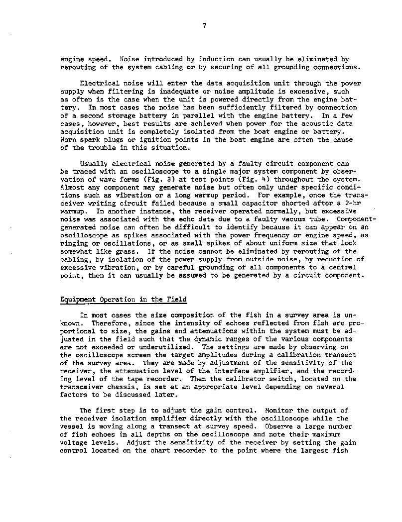
Usually electrical noise generated by a faulty circuit component canbe traced with an oscilloscope to a single major system component by obser-vation of wave forms Fig. 3! at test points Fig. 0! throughout the system.Almost any component may generate noise but often only under specific condi-tions such as vibration or a 3.ong warmup period. For example, once the trans-ceiver writing circuit failed because a small capacitor shorted after a 2-hrwarmup. In another instance, the receiver operated normally, but excessivenoise was associated with the echo data due to a faulty vacuum tube. Component-generated noise can often be difficult to identify because it can appear on anoscilloscope as spikes associated with the power frequency or engine speed, asringing or oscillations, or as small spikes of about uniform size that looksomewhat like grass. If the noise cannot be eliminated by rerouting of thecabling, by isolation of the power supply from outside noise, by reduction ofexcessive vibration, or by careful grounding of all components to a centralpoint, then it can usually be assumed to be generated by a circuit component.

E ui ment 0 ration in the Field

In most cases the size composition of the fish in a survey area is un-known. Therefore, since the intensity of echoes reflected from fish are pro-portional to size, the gains and attenuations within the system must be ad-justed in the field such that the dynamic ranges of the various componentsare not exceeded or underutilized. The settings are made by observing onthe oscilloscope screen the target amplitudes during a calibration transectof the survey area. They are made by adjustment of the sensitivity of thereceiver, the attenuation level of the interface amplifier, and the record-ing level of the tape recorder. Then the calibrator switch, located on thetransceiver chassis, is set at an appropr iate level depending on severalfactors to be discussed later.

The first step is to adjust the gain control. Monitor the output ofthe receiver isolation amplifier directly with the osci3.loscope while thevessel is moving along a transect at survey speed. Observe a large numberof fish echoes in all depths on the oscilloscope and note their maximumvoltage levels. Adjust the sensitivity of the receiver by setting the gaincontrol located on the chart recorder to the point where the largest fish

OSCILLOSCOPE DISPLAY

CALIBRATI CNSIGNAL

+I IW

10$ INK

-I MV

50 os

+IV

+ I V

� I V

l00 ms

+ I V

Fig. 3. Typical test waveforms as viewed on an oscilloscopeat the indicated system test points.

3,4,5

$05 kEK

TvG curve !

tp

tp

tp

to

+SO V

+I V

VGICZ FRZQUZNCT

-I V

� 4V

0

+IV

VOICE FREgUZNCTl0

-4V

+RV

9,10

0

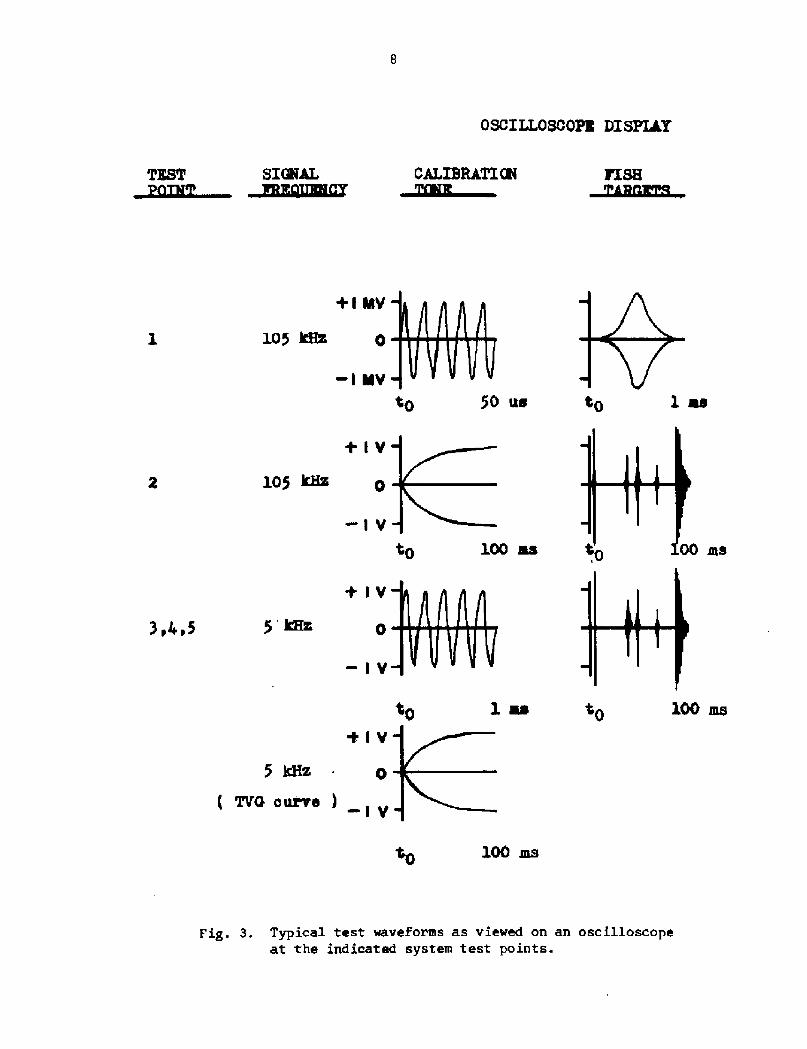
Fig. 3. Typical test waveforms as viewed on an oscilloscopeat the indicated system test points � continued.

2,4,S or 16 / aeeea4

1 / mamsMXTVm an.ee

1 / T$tJQIBMKFZZD PtKSR

to

t0

10

OUT%%ITSZCEO SOUNDER

SIGNAL

2

6

7

g SXCNAL MONITOR

IO

9 SnrC MCmnoa

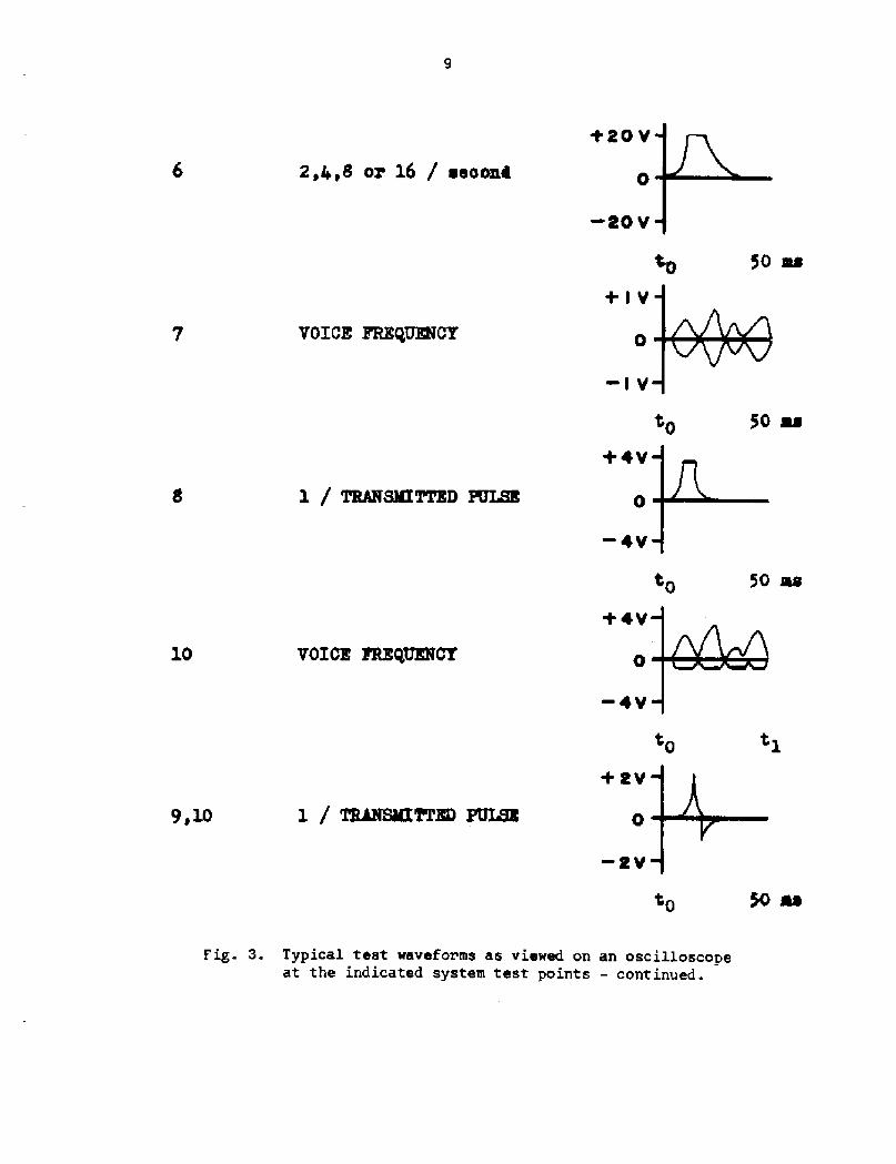
Fig. 0, Black diagram of the data acquisition unit showingthe various test points.

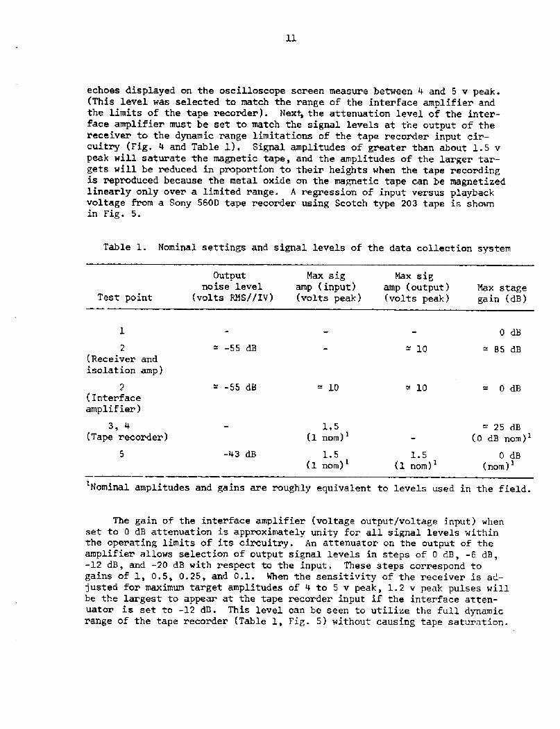
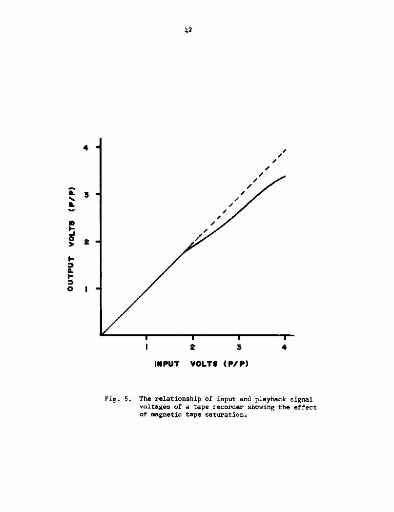
echoes displayed on the oscilloscope screen measure between 4 and 5 v peak. This level was selected to match the range of the interface amplifier andthe limits of the tape recorder!. Next, the attenuation level of the inter-face amplifier must be set to match the signal levels at the output of thereceiver to the dynamic range Limitations of the tape recorder input cir-cuitry Fig. 4 and Table 1!. Signal amplitudes of greater than about 1.5 vpeak will saturate the magnetic tape, and the amplitudes of the larger tar-gets will be reduced in proportion to their heights when the tape recordingis reproduced because the metal oxide on the magnetic tape can be magnetizedlinearly only over a limited range. A regression of input versus pI.aybackvoltage from a Sony 560D tape recorder using Scotch type 203 tape is shownin Fig. 5.

Table 1. Nominal settings and signal levels of the data collection system

Output Max sig Max s ignoise level amp input! amp output! Max stage

volts RMS//IV! volts peak! volts peak! gain dB!Test point

0 dB

-55 dB2

Receiver andisolation amp!

10 85 dB

" --55 dB 10 10 0 dB2 Interfaceamplifier!

1,5

� nom!3

Tape recorder!25 dB

� dB nom!

-43 dB 1.5

� nom!1.5

� nom!0 dB

nom!'

The gain of the interface amplifier voltage output/voltage input! whenset to 0 dB attenuation is approximately unity for all signal levels withinthe operating limits of its cix'cuitry. An attenuator on the output of theamplifier allows selection of output signal levels in steps of 0 dB, -6 dB,-12 dB, and -20 dB with respect to the input. These steps correspond togains of 1, 0.5, 0.25, and 0.1. When the sensitivity of the receiver is ad-justed for maximum target amplitudes of 4 to 5 v peak, 1.2 v peak pulses willbe the largest to appear at the tape recorder input if the interface atten-uator is set to -12 dB. This level can be seen to utilize the full dynamicrange of the tape recorder Table 1, Fig. 5! without causing tape saturation.

'Nominal amplitudes and gains are roughly equivalent to levels used in the field.

12

a

0 I

2 3

INPVT VOLTS P/ P!

Fig. 5. The relationship of input and playback signalvoltages of a tape recorder showing the effectof magnetic tape saturation.

13

Further, to adjust the record level of the tape recorder, observe theinput and output voltages of the calibration oscillator signal with the oscil-loscope Fig. 3, test points 3 and 5!, and adjust the right signal! channelrecord level for equal input and output calibration oscillator voltage readings,Finally, set the left channel synchronization pulse! record level such that thepositive portion of the sync pulse is about 2 vp. A higher setting will causecross talk between the right and left channel, and this will interfere withanalysis of the recorded data. Cross talk in the tape recorder will be discus-sed later. Tape speed on this system has been most often set at 9.5 cm/sec�-3/4 IPS! because frequency response is adequate and tape usage is minimal.At slower tape speeds frequency response is inadequate.

Select the best setting of the calibration oscillator and measure its amp-litude with the transducer submerged. The ideal setting of the calibrationoscillator amplitude is such that its peak voltage out of the receiver is simi-lar to the fish target voltage amplitudes at corresponding depths, where depthis measured by elapsed time after the transmitter pulse �.37 ms/meter!. Onlytwo calibration levels, 100 and 1,000 uv, are available, so the usual proce-dure is to select the largest calibration oscillator output level that doesnot exceed the dynamic range limitations of the system at the maximum depthof interest within the survey area.

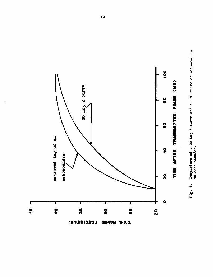
The circuitry of the echo sounder receiver includes a 20 log R R = depthin meters! time varied gain TVG! control circuit Fig. 6!; therefore, sincethe output of the calibration oscillator is applied to the input of the re-ceiver, the TVG curve, representing the increase in gain with depth, can beviewed directly on an oscilloscope as peak calibrator voltage versus timeafter the transmitted pulse. The gain of the receiver amplifier can be calcu-lated for any depth from the TVG curve since both the input voltage the cali-bration oscillator output! and the output voltage are known. The oscillatoroutput is calibrated in rms root mean square! voltage v = 0.707 vp!;therefore the voltage of the TVG curve at the time t. musie converted torms voltage also. The equation used to calculate receiver gain in decibels dB! is as follows:

v outputdB = 20 log

v inputrms

E

or dB = 20 logl0 Z !1

After selecting a calibrator level, record in a field log its peak volt-age at some reference time after the transmitter pulse e.g., 50 ms! for useduring data analysis. Record the calibration voltage on the magnetic tapeperiodically throughout the survey as it will show any system anomalies orgain changes from such operational problems as low power supply voltages orcomponent failure.

O O

R

R

ae

0

0 Oi

g1QQIQRQ ! 3%Nil 8 A L

qjF-

IO

0 C nj

O Plnl Se

W 'd0 g

09 ol

0

tO Og CI0 g

15

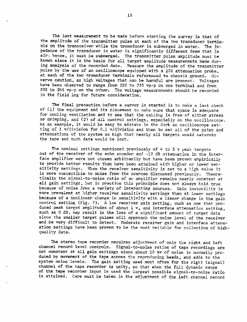
The last measurement to be made before starting the survey is that ofthe amplitude of the transmitter pulse at each of the two transducer termin-als on the transceiver while the transducer is submerged in water. The im-pedance of the transducer in water is significantly different from that inair; hence, it must be submerged. The transmitter pulse amplitude must beknown since it is the basis for all target amplitude measurements made dur-ing analysis of the recorded data. Measure the amplitude of the transmitterpulse by the use of an oscilloscope equipped with a 10X attenuation probe,at each of the two transducer terminals referenced to chassis ground. Ob-serve caution, as high voltages that can be harmful are present. Voltageshave been observed to range from 220 to 235 vp-p on one terminal and from230 to 245 vp-p on the other. The voltage measurements should be recordedin the field log for future consideration.

The final precaution before a survey is started is to make a last checkof l! the equipment and its placement to make sure that space is adequatefor cooling ventilation and to see that the cabling is free of either stressor crimping, and �! of all control settings, especially on the oscilloscope.As an example, it would be easy to mistake in the dark an oscilloscope set-ting of l v/division for 0.1 v/division and then to set all of the gains andattenuations of the system so high that nearly all targets would saturatethe tape and much data would be lost.

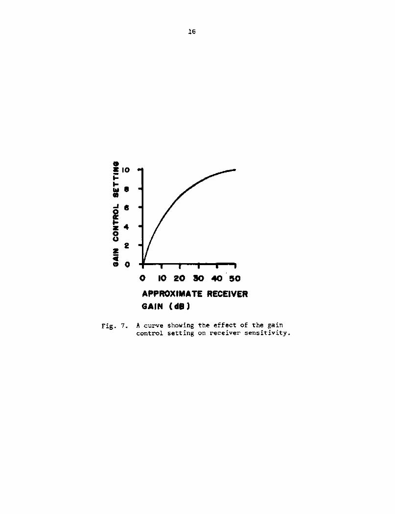
The nominal settings mentioned previously of 4 to 5 v peak targetsout of the receiver of the echo sounder and -12 dB attenuation in the inter-face amplifier were not chosen arbitrarily but have been proven empiricallyto provide better results than have been attained with higher or lower sen-sitivity settings. When the receiver sensitivity is set to a high value itis more susceptible to noise from the sources discussed previously. Theore-tically the signal-to-noise ratio of an amplifier remains nearly constant atall gain settings, but in practice this principle does not always hold truebecause of noise from a variety of interacting sources. Gain instability ismore prevalent at higher receiver sensitivity settings than at lower settingsbecause of a nonlinear change in sensitivity with a linear change in the gaincontrol setting Fig. 7!. A low receiver gain setting, such as one that pro-duced peak target amplitudes of about 1 v, and interface attenuation setting,such as 0 dB, may result in the loss of a significant amount of target datasince the smaller target pulses will approach the noise level of the receiverand be very difficult to detect. Moderate receiver gain and interface attenu-ation settings have been proven to be the most reliable for collection of high-quality data.

The stereo tape recorder requires adjustment of only the right and leftchannel record level controls. Signal-to-noise ratios of tape recordings arenot constant at all gain settings since about 10 mv of noise is normally pro-duced by movement of the tape across the reproducing heads, and adds to thesystem noise levels. The gain setting used most often for the right signal!channel of the tape recorder is unity, so that when the full dynamic rangeof the tape recorder input is used the largest possible signal-to-noise ratiois attained. Care must be taken in the adjustment of the left channel record

I aio

I tu 8

~e

O g 10 CP

RR

C 4 0 iO aa So 4050APPROXIMATE RKCKlVKR

OAKEN ai!

Fig. 7. A curve shoving the effect of the gaincontrol setting on receiver sensitivity.

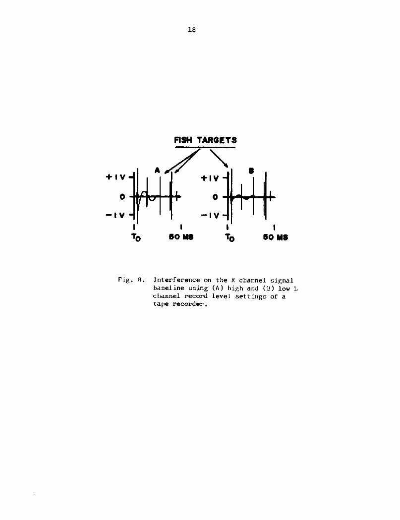
level, as cross talk between the two channels can occur. The sync pulse ap-plied to the input of the left channel of the recorder is in the order of 4 vp Fig. 4, TP $8!. This amplitude can drive the recorder input far into tapesaturation, but since the sync pulse is used only for a timing reference forthe transmitter pulses, no data are lost. interference is generated in thesignal channel by this pulse, however; it appears as a Low-frequency, dampedringing with a periodicity of about 15 to 20 ms. Apparently this effect iscaused by inadequate filtering of the power supply within the tape recorderand is coupled in this way from the left to the right channel. The problemexists only when the left channel amplifier is very much overdriven and isnot an indication of poor circuit design. An example of the effects of highand low left channel recording levels on the right channel output is shownbelow as it would appear on an oscilloscope Fig. 8, Fig. 4 - test point 5!.

The Digital Data Anal sis Unit DDAU!

General Descr iption

The estimation of fish densities by echo integration is based on thesummation of echo intensities from a number of targets detected within anydefined sample volume, and division of this by the average echo intensityfrom a single fish. The techniques for estimation of fish densities and themathematics of echo integration have been described Moose et al., l971a;Moose et al., L9715; Ehrenberg and Lytle, l971; Ehrenberg, l972!. A corn-puter program used by the Digital Data Analysis Unit for estimation of fishdensity by integration has been described Noose et al., 1971a!. The actualoperation of the Digital Data Analysis Unit DDAU! has not been well described.A discussion of the overaLL data analysis system follows.

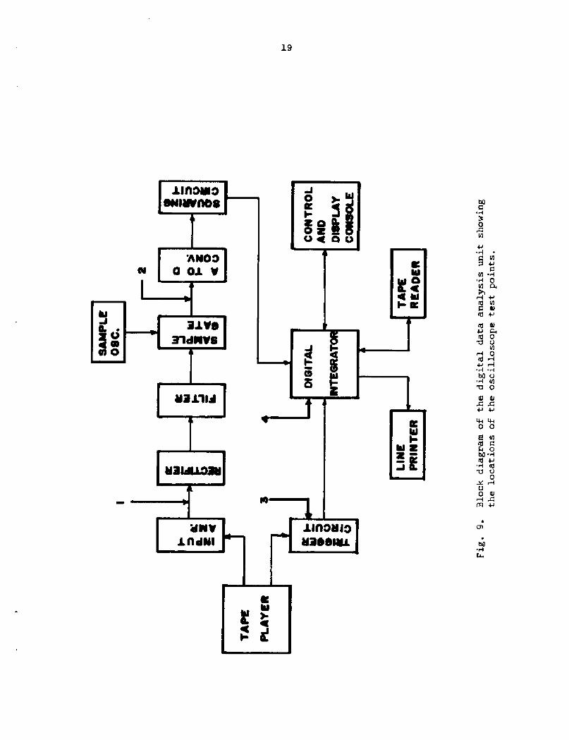
The Digital Data Analysis Unit is composed of a number of interconnect-ing components. A block diagram of the system showing the interconnectionsbetween each component, the data flow paths and four test points, is givenin Fig. 9. A brief description of the operation of each block will begiven, followed by a detailed discussion of each under their appropriateheadings'

The first black box that a piece of data will encounter as it is passedDigital Data Analysis Unit is an input amplifier. This circuit

has a variable gain and its purpose is to provide adjustment of target vol-tages of a wide range to arange of amplitudes best suited to the analysisunit circuitry. This unit interfaces input data to the processing unit.

A rectifier, filter and sampling circuit follow the input amplifier.The purpose of these three boxes are to envelope detect the target reflec-tion pulses, to filter out most of the 5 kHz input frequency component, andto sample the detected voltage pulse at a predetermined rate. The input to

FISH TANOKTS

interference on the R channel signalbaseline using A! high and U! low Lchannel record level settings of atape recorder.

I

50 MO

I

ToI

50 MS

30

Vp4 ~

5

Vnj Vlg S

tg Ol

0o

pqj W

0 pCl Ill

W

0 0Ol

4 ob0 '8

�'U U

0

Up cl

20

the rectifier or envelope detector consists of amplitude modulated trainsof 5 kHz sine waves, whose envelopes or outlines represent target reflec-tions . Because of this, rectification and filtering are necessary to avoidvoltage measurements being made by the sampling circuit at random points onthe 5 kHz sine waves, rather than at the true amplitude of the pulse envelopesat the sampled points. A more detailed discussion is given in the followingtext.

An analog-to-digital converter follows the sampling circuit in the dataflow path The purpose for this box is to convert the analog voltage measure-ments to interface the analog input data and the digital computer-integrator.Digital data is also desirable because it can be manipulated, transformed,etc. with great precision and is not affected by gain, frequency characteris-tics, or other analog circuitry drawbacks,

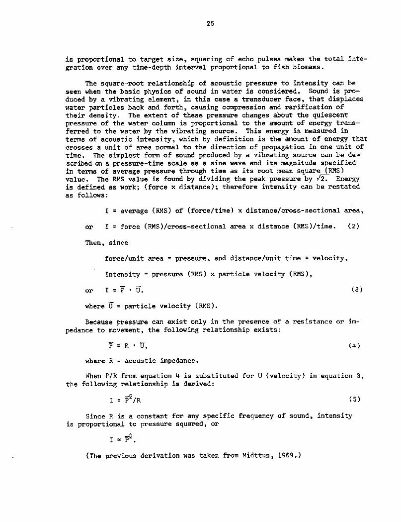
Immediately following the A to D converter in the data analysis unit isa digital squaring circuit whose function it is to square each digital vol-tage measurement from the sampling circuit through the A to D converter.Squaring is necessary, since conversions to voltage pulses from acoustic echointensities by the transducer, are proportional to the square root of the echointensities. Therefore, squaring of the voltage measurements normalizes themto the original target reflection intensities, which in turn are directly pro-portional to the biomass of the reflecting targets. A detailed descriptionof the physics involved is given in the following text.

The final signal processing block in the analysis unit is the digitalintegrator. Each squared voltage measurement is stored in one of nine sum-ming cells representing depth strata. After a predetermined interval of time,the sums of the voltage measurements in each cell are automatically outputed,and are proportional to the total biomass of all targets detected in eachdepth-time interval. The following sections give more detailed discussions ofthe various DDAU components.

Detailed Descri tions of the DDAU Com onents and 0 erations

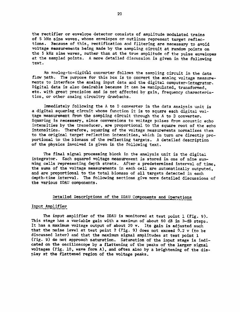
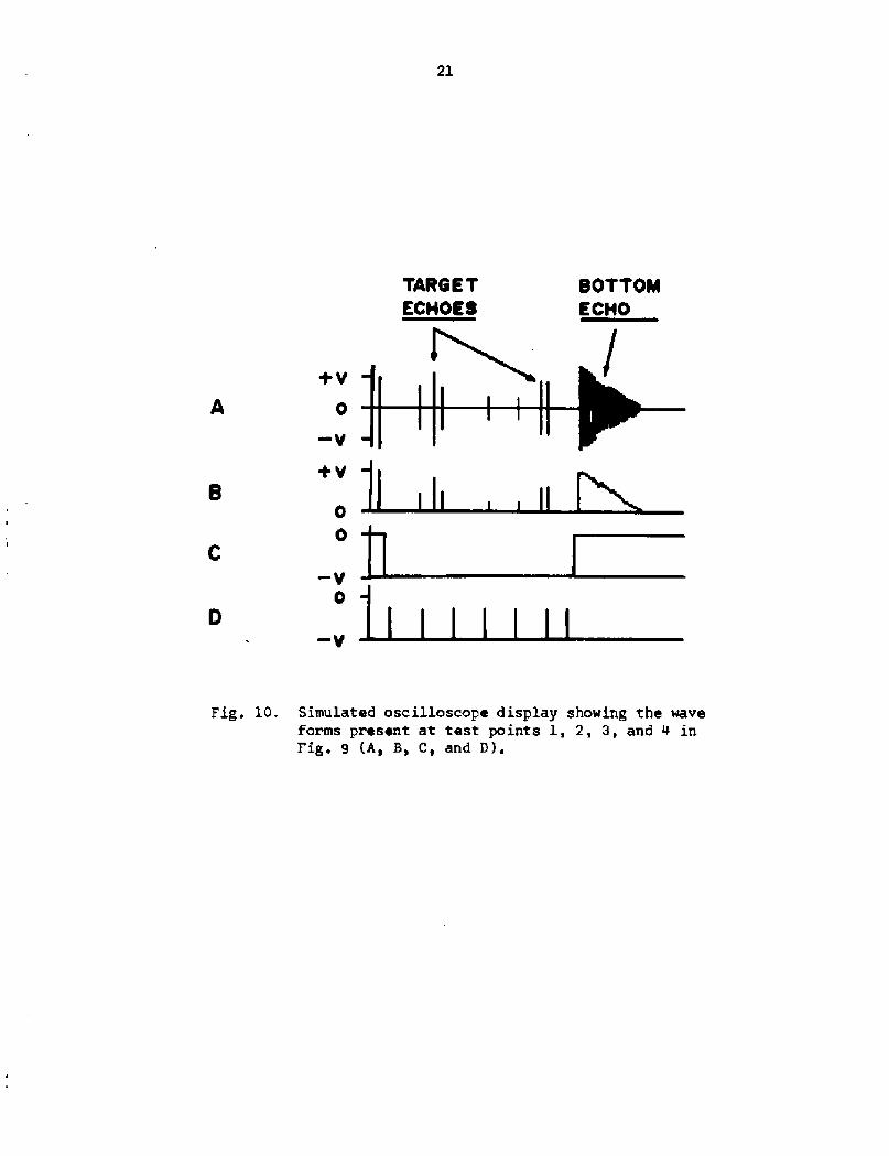
The input amplifier of the DDAU is monitored at test point l Fig. 9!.This stage has a variable gain with a maximum of about 60 dB in 3-dB steps.It has a maximum voltage output of about 20 v. Its gain is adjusted suchthat the noise level at test point 2 Fig. 9! does not exceed 0.2 v to bediscussed later! and that the maximum signal amplitudes at test point 1 Fig. 9! do not approach saturation. Saturation of the input stage is indi-cated on the oscilloscope by a flattening of the peaks of the larger signalvoltages Fig. 10, wave form A!, and often also by a brightening of the dis-play at the flattened region of the voltage peaks.

+V

0

Fig. 10. Simulated oscilloscope display showing the waveforms present at test points l, 2, 3, and 0 inFig. 9 A, 3, C, and D!.

0 0

TARGE T

ECHOEI

BOTTOMECHO

22

Rectifier

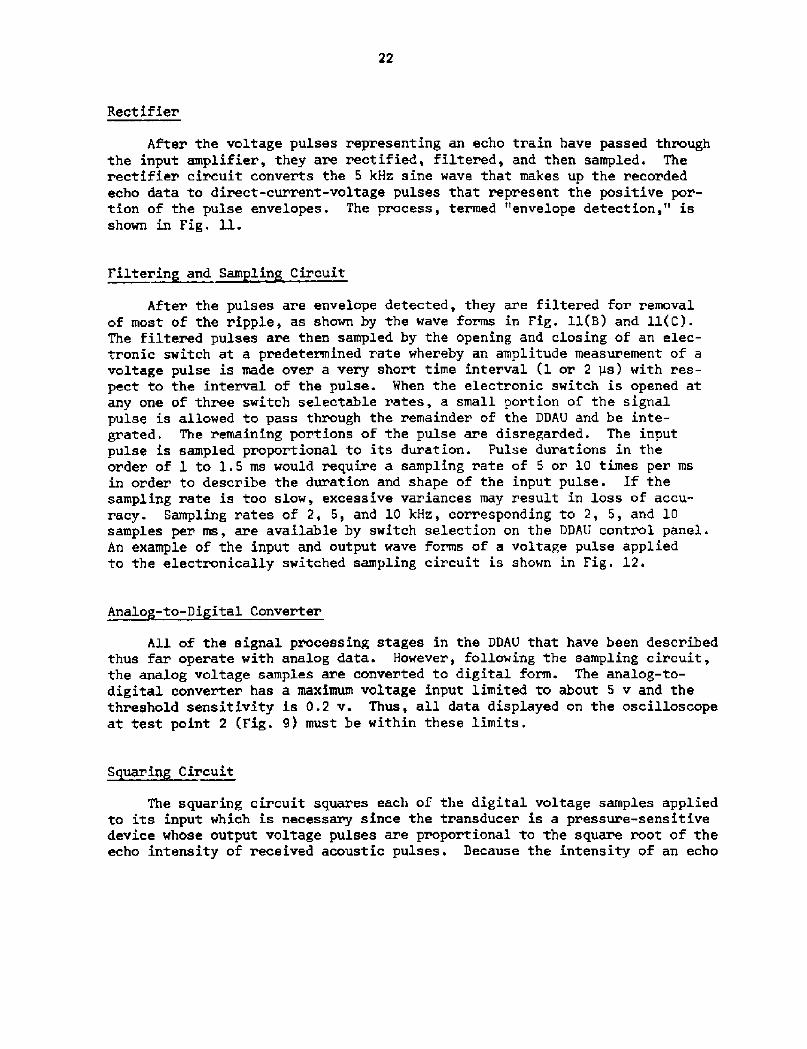
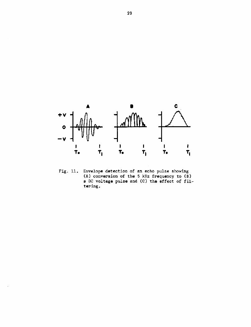
After the voltage pulses representing an echo train have passed throughthe input amplifier, they are rectified, filtered, and then sampled, Therectifier circuit converts the 5 kHz sine wave that makes up the recordedecho data to direct-current-voltage pulses that represent the positive por-tion of the pulse envelopes. The process, termed "envelope detection," isshown in Fig. 11.

Filterin and Sam lin Circuit

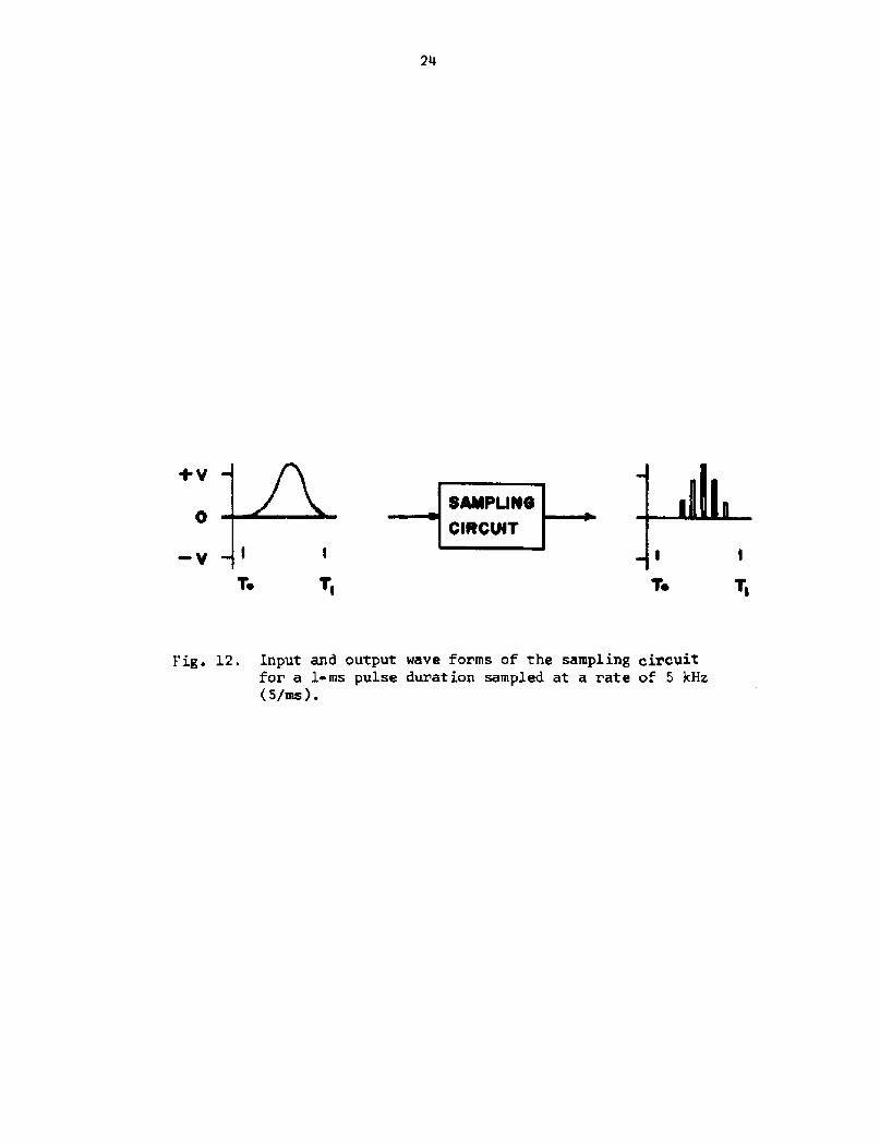
After the pulses are envelope detected, they are filtered for removalof most of the ripple, as shown by the wave forms in Fig. 11 B! and ll C!.The filtered pulses are then sampled by the opening and closing of an elec-tronic switch at a predetermined rate whereby an amplitude measurement of avoltage pulse is made over a very short time interval � or 2 ps! with res-pect to the interval of the pulse. When the electronic switch is opened atany one of three switch selectable rates, a small portion of the signalpulse is allowed to pass through the remainder of the DDAU and be inte-grated. The remaining portions of the pulse are disregarded. The inputpulse is sampled proportional to its duration. Pulse durations in theorder of 1 to 1.5 ms would require a sampling rate of 5 or lO times per msin order to describe the duration and shape of the input pulse . If thesampling rate is too slow, excessive variances may result in loss of accu-racy. Sampling rates of 2, 5, and 10 kH2,, corresponding to 2, 5, and 10samples per ms, are available by switch selection on the DDAU control panel.An example of the input and output wave forms of a voltage pulse appliedto the electronically switched sampling circuit is shown in Fig. 12.

Analog-to-Digital Converter

All of the signal processing stages in the DDAU that have been describedthus far operate with analog data. However, following the sampling circuit,the analog voltage samples are converted to digital form. The analog-to-digital converter has a maximum voltage input limited to about 5 v and thethreshold sensitivity is 0.2 v. Thus, all data displayed on the oscilloscopeat test point 2 Fig. 9! must be within these limits.

S uarin Circuit

The squaring circuit squares each of the digital voltage samples appliedto its input which is necessary since the transducer is a pressure-sensitivedevice whose output voltage pulses are proportional to the square root of theecho intensity of received acoustic pulses. Because the intensity of an echo

23

+V

Fig. 11. Envelope detection of an echo pulse showing A! conversion of the 5 kHz frequency to B!a DC voltage pulse and C } the ef f ect of f il-tering.

I I

Te TII

Te

24

TI Te

Fig. 12. Input and output wave forms of the sampling circuitfor a I-ms pulse duration sampled at a rate of 5 kHz�/ms!.

25

is proportional to target size, squaring of echo pulses makes the total inte-gration over any time-depth interval proportional to fish biomass.

The square-root relationship of acoustic pressure to intensity can beseen when the basic physics of sound in water is considered. Sound is pro-duced by a vibrating element, in this case a transducer face, that displaceswater particles back and forth, causing compression and rarification oftheir density. The extent of these pressure changes about the quiescentpressure of the water column is proportional to the amount of energy trans-ferred to the water by the vibrating source. This energy is measured interms of acoustic intensity, which by definition is the amount of energy thatcrosses a unit of area normal to the direction of propagation in one unit oftime. The simplest form of sound produced by a vibrating source can be de-scribed on a pressure-time scale as a sine wave and its magnitude specifiedin terms of average pressure through time as its root mean square RMS!value. The RHS value is found by dividing the peak pressure by ~2. Energyis defined as work; force x distance!; therefore intensity can be restatedas follows.

I = average RMS! of force/time! x distance/cross-sectional area,

or I = force RMS!/cross-sectional area x distance RMS!/time. �!

Then, since

force/unit area = pressure, and distance/unit time = velocity,

Intensity = pressure RMS! x particle velocity RMS!,

�!or I = P ~ U.

where U = particle velocity RMS!.

Because pressure can exist only in the presence of a resistance or im-pedance to movement, the following relationship exists:

P=R'U,

where R = acoustic impedance.

When P/R from equation 4 is substituted for U velocity! in equation 3,the following relationship is derived:

I=P/R

Since R is a constant for any specific frequency of sound, intensityis proportional to pressure squared, or

I-"P

The previous derivation was taken from Midttun, 1969.!

26

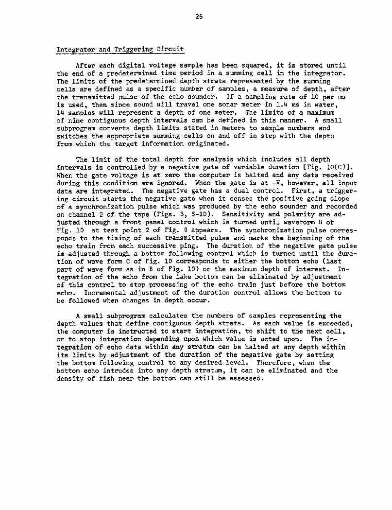
Inte ator and Tri erin Circuit

After each digital voltage sample has been squared, it is stored untilthe end of a predetermined time period in a summing cell in the integxator.The limits of the predetermined depth strata represented by the summingcells are defined as a specific number of samples, a measure of depth, afterthe transmitted pulse of the echo sounder. If a sampling rate of 10 per msis used, then since sound will travel one sonar meter in L.4 ms in water,L4 samples will repx'esent a depth of one meter. The limits of a maximumof nine contiguous depth intervals can be defined in this manner. A smallsubpxogram converts depth Limits stated in meters to sample numbers andswitches the appropriate summing cells on and off in step with the depthfrom which the target information originated.

The limit of the total depth for analysis which includes all depthintervals is controlled by a negative gate of variable duration t Fig, 10 C!],When the gate voltage is at zero the computer is halted and any data receivedduring this condition are ignored. When the gate is at -V, however, all inputdata are integrated. The negative gate has a dual control. First, a trigger-ing circuit starts the negative gate when it senses the positive going slopeof a synchronization pulse which was produced by the echo sounder and recordedon channel 2 of the tape Figs. 3, 5-l0!. Sensitivity and polarity are ad-justed through a front panel control which is turned until waveform B ofFig. 10 at test point 2 of Fig. 9 appears. The synchronization pulse corres-ponds to the timing of each transmitted pulse and marks the beginning of theecho tx'ain from each successive ping. The duration of the negative gate pulseis adjusted through a bottom following control which is turned until the dura-tion of wave form C of Fig. 10 corresponds to either the bottom echo lastpart of wave form as in B of Fig. 10! or the maximum depth of interest. In-tegration of the echo from the lake bottom can be eliminated by adjustmentof this control to stop processing of the echo train just before the bottomecho. Incremental adjustment of the duration control a11ows the bottom tobe followed when changes in depth occur.

A small subprogram calculates the numbers of samples representing thedepth values that define contiguous depth strata. As each value is exceeded,the computer is instructed to start integration, to shift to the next cell,or to stop integration depending upon which value is acted upon. The in-tegration of echo data within any stratum can be halted at any depth withinits limits by adjustment of the duration of the negative gate by settingthe bottom following control to any desired level. Therefore, when thebottom echo intrudes into any depth stratum, it can be eliminated and thedensity of fish near the bottom can still be assessed.

27

Control Console, Ta Reader, and Line Pz'inter

The control console is the input device by which all of the necessarypaz'ameters for the program can be entered into the DDAU computer. The pro-gram is stored on magnetic tape and is initiated by a basic command thatis toggled into the computer by front panel switches. When the appropriatememory location is called and the computez' is started, a small program isinitiated that commands the tape reader to read the DDAU progz am into thememory. When this is completed, a series of questions is sequentially dis-played on the control console screen. The answers to these questions areof two types; some are for operator zeference and are not entered into theprogram and the rest are parameters necessary for the various computationsto be done by the computer. The questions asked by the DDAU before inte-gration can be started, and their explanations are given below.

l. Date today?

2. Run identification?

3. Operator?

Questions 1-3 are for the operator's use only and do not ask For pro-gram parameters. Each of the questions must be answered by at least onealphanumeric character, however, before the next question will be displayed.

4. Number of sounders operating?

The DDAU can integrate data received from two sounders operating simul-taneously by integrating alternate pulses. A complete set of depth strataand separate outputs are automatically printed foz each sounder input- Thedepth strata and overall depth interval must be identical for both sounders,however. The answer to question 4 must be l or 2.

S. Ping rate?

Question 5 is for use by the operator for his records and does notask for an input parameter. The ping rate is the rate at which the echosounder is pulsed. In most instances the ping rate is 2 or 3 per second,and is determined by the design of the echo sounder used to collect data.

6. What sampling rate is set?

This question is also for use by the operator and is not an inputparameter. The sampling rate is selected by means of a front panel con-trol as described previously.

7. Number of pings for this run?

28

The number of pings for a run, since each transmitted ping occurs ata regular interval, is used as a time measurement of a transect section orrun. As an example, if a sounder pings twice per second, 600 pings wouldrepresent a 5-min section of a transect. The answer to this question canbe any integer.

8 ~ List values of' A?

The value of A is a program parameter that defines the r'elationshipof transmitted acoustic intensity, the sensitivity of the receiver, thedirectivity function of the transducer, the average target strength ofthe fish of interest, and various other parameters Moose et al., 1971!.The value of A must be calculated, or at least estimated, prior to inte-gration such that a specific value can be entered.

9. Number of depth values'?List depth valuesList values of B for sounder oneList values of B for sounder two

What buffer size?

The answer to the first part of this question is the number of depthvalues defining the contiguous depth strata of interest. The maximumnumber of depth values is 10.

In answer to the second part of question 9, list the consecutivedepth values in m! that define the limits of each stratum of interest.

The values of B for sounders one and two are related to the absorp-tion of sound in water at the operating frequency, the gain of the sounderwith respect to that at 100 ms includes TVG circuit and is a function oftime!, and the travel time of sound through the stratum of interest. Ei-ther 1 or 2 values of B must be entered for each stratum depending uponthe number of sounders operating question 4!.

The buffer size defines a depth stratum between the end of the nega-tive gate that limits the overall depth interval and the last sample ineach echo train that is integrated LFig. 10 E!]. The negative gate pulseduration can be set by use of the bottom following control to coincide withthe bottom echo and the buffer interval prevents integration of noise veryclose to the bottom echo. The buffer size is given in meters and may be ofany size. In most cases a buffer size of 5 to 7 m has been found to beadequate.

10. What is TP[Cj?

This value is the initial depth in meters at which the bottom will beencountered. After integration is started, the bottom following pulse[Fig. 11 C!] is adjusted by use of the bottom following control to instructthe computer, ping by ping, as to the current depth.

29

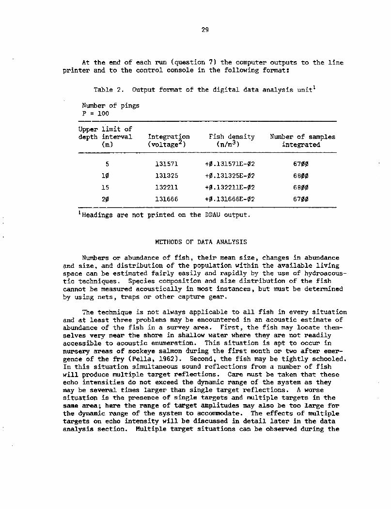
At the end of each run question 7! the computer outputs to the lineprinter and to the control console in the following format!

Table 2. Output format of the digital data analysis unit

Number of pingsP=100

Upper limit ofdepth interval

m!Integrat ion voltage2!

Fish density n/m3!

Number of samplesintegrated

+8.131571E-H2

+g.l31325E-I|I2

+5.132211E-g2

t8.131666E-g2

6755

68I58

6858

6758

131571

131325

1322ll

131666

15

'Headings are not printed on the DDAU output.

METHODS OF DATA ANALYSIS

The technique is not always applicable to all fish in every situationand at least three problems may be encountered in an acoustic estimate ofabundance of the fish in a survey area. First, the fish may locate them-selves very near the shore in shallow water where they are not readilyaccessible to acoustic enumeration. This situation is apt to occur innuxs*ry areas of sockeye salmon during the first month or two after emer-gence of the fry Pella, l962!. Second, the fish may be tightly schooled.In this situation simultaneous sound reflections from a number of fish

will produce multiple target reflections. Care must be taken that theseecho intensities do not exceed the dynamic range of the system as theymay be several times larger than single target reflections. A worsesituation is the presence of single targets and multiple targets in thesame area; here the range of target amplitudes may also be too large forthe dynamic range of the system to accommodate. The effects of multipletargets on echo intensity will be discussed in detail latex in the dataanalysis section. Multiple target situations can be observed during the

Numbers ox abundance of fish, their mean size, changes in abundanceand size, and distribution of the population within the available livingspace can be estimated fairly easily and rapidly by the use of hydroacous-tic techniques. Species composition and size distribution of the fishcannot be measured acoustically in most instances, but must be determinedby using nets, traps or other capture gear.

30

day in nearly any sockeye salmon nursery area since they commonly schooltightly during this time at depths of from about 45 to 60 m. At the on-set of darkness, the schools break up and the fish move toward the surface.Because of these problems, acoustic surveys of juvenile sockeye salmonhave always been conducted at night.

A similar problem arises when the fish are stratified by size throughthe water column. This situation was observed on severa1 occasions whenadult and juvenile sockeye salmon were present in a lake and when finger-lings, fry, and other larger resident fish were distributed at differentdepths Dawson, 1972!. Adults can have as much as 20 dB larger targetstrength than juvenile salmon. Since the overall span of target ampli-tudes from these fish can exceed the average target strength by another10 dB, the range of target data can be as great as 40 dB. Such a rangeis very difficult to work with; therefore two similar surveys can bemade of the lake, one at a high receiver sensitivity, the other at alower sensitivity. When the high receiver sensitivity is used, thegain must be adjusted such that the amplitudes of the juvenile salmontargets utilize the full dynamic range of the data collection system.Then the adult salmon targets will nearly all cause tape saturation tosuch an extent that when the tape is reproduced the reflections fromadults will not be much larger than those from the juveniles. The op-posite effect will occur when receiver gain is reduced to a level thatlimits the amplitudes of the adult salmon targets to the dynamic rangeof the system. In this case, most of the juvenile salmon targets willbe very small and a large portion will be lost in the normal noise levelof the system. The situation is similar although not so extreme whenfry 0 age class! and fingerlings� year age class! stratify themselvesby depth and sometimes distribute themselves by area. Careful attentionmust be paid to target amplitudes during an acoustic survey in such asituation so that either tape saturation or loss of data in the ambientnoise level from the system is avoided.

Estimation of Effective Sam le Volume b the Use of an Oscillosco e

When the face of a transducer is submerged and pulsed, acoustic energyis transmitted to all points in the water within the polar coordinates r, 6, f!. The symbol r represents a measure of distance from the trans-ducer face to the maximum depth of interest, 8 = 0 to 90o and $ = Oo to 360 Fig. 13!.

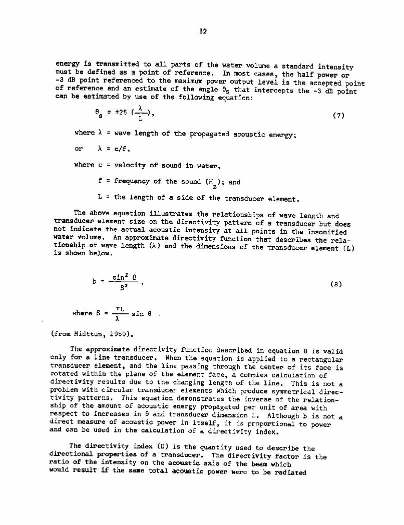
Although acoustic energy is propagated from a transducer to all partsof the aforementioned water volume, the intensities of the energy per unitof area for all angles 0 and rIr, given any specific r, are not equivalent butare determined by several physical properties of the transducer. Instead,the energy is distributed mostly near r, 0, 0! and decreases rapidly as 0increases with respect to the acoustic axis of the transducer. Since some

F'ig. l3. Illustration of the polar coordinate system used inthe def inition of the directivity function of atransducer.

32

8 = +2S !,s

whez'e X = wave length of the propagated acoustic energy;

or X = c/f,

where c = velocity of sound in water,

f = frequency of the sound H !; andz

L = the length of a side of the transducer element.

The above equation illustrates the relationships of wave length andtransducez' element size on the directivity pattern of' a transducer but doesnot indicate the actual acoustic intensity at all points in the insonifiedwater volume. An approximate directivity function that describes the rela-tionship of wave length A ! and the dimensions of the transducer element L!is shown below.

b sin Bp2 8!

TlLwhere 8 = sin 8

fram Midttun, l969! ~

The approximate directivity function described in equation 8 is validonly for a line transducez'. When the equation is applied to a rectangulartransducer element, and the line passing through the center of its face isrotated within the plane of the element face, a complex calculation ofdirectivity results due to the changing length of the line. This is not apzoblem with circular transducer elements which produce symmetrical direc-tivity patterns. This equation demonstrates the inverse of the relation-ship of the amount of acoustic energy propagated per unit of area withrespect to increases in 0 and transducer dimension L. Although b is not adirect measure of acoustic power in itself, it is proportional to powezand can be used in the calculation of a directivity index.

The directivity index D! is the quantity used to describe thedirectional properties of a tzansducer. The directivity factor is theratio of the intensity on the acoustic axis of the beam whichwould result if the same total acoustic power were to be radiated

energy is transmitted to all parts of the water volume a standard intensitymust be defined as a point of reference. In most cases, the half power oz-3 dB point z'eferenced to the maximum power output level is the accepted pointof reference and an estimate of the angle 8s that intercepts the -3 dB pointcan be estimated by use of the following equation:

33

uniformly in all directions. As an example, the directivity index of anideal hemisphez ical transducer element is 0.5. The equation used to cal-culate the directivity index of a transducer is given below.

D = 10 log10 f~ b + dp!1 -110 um 9!

wheze b is defined by equation 8.

A useful approximation to the directivity index can be calculated withthe following equation.

D = 10 log4TiA

where A = area of the transducer face

9a !

= acoustic wave length

from Midttun, 1969!.

The directivity pattern Fig. 15! describes the distribution of acousticenergy about the axis of the transducer but does not indicate the factorsthat define the limits of target detectability. It has been shown by thedirectivity index Equation 9! that, since there are no range or angular limi-tations in this function, acoustic enez'gy is tz'ansmitted in varying amountsto all parts of the entire water volume each time that the transducer ispulsed; therefore, reflections from all density discontinuities throughoutthe entire water volume must return to the transducer in varying intensities.When the question of target detectability is approached in this manner, itcan be seen that the only limiting factors are the sensitivity of the receiverand the noise levels associated with the target data. Since the dynamic rangeof the data collection system limits maximum sensitivity and a relatively con-stant noise level is assoiated with target data reproduced from tape record-ings, a fairly distinct continuum can be described which is in actuality theeffective pulse sample volume.

A pulse of acoustic energy produced by a transducer will spread through-out the water column in the manner described by the square law. The samephenomenon occurs as energy is reflected from a target and travels hack

At this point it can be seen that the intensity of the acoustic energypropagated throughout an insonified watez volume fzom a transducer is depen-dent upon a variety of physical properties of the element. In practice sincethe previously described equations are insensitive to anomalies in a trans-ducer construction, or operating characteristics, directivity of a tzansduceris measured in the laboratory by applying a signal of constant amplitude atthe operating frequency of the element to its input terminals and by measur-ing the intensity of the acoustic energy produced in water at a standard dis-tance and at all angles e. Fig. 1% shows such a measurement setup and Fig. 15shows the resulting directivity pattern as would be measured by the test setup.Under normal conditions, the operating characteristics of a transducer arestable for a long period of time.

3g 0~ Q

Oqj

j

~ rfV 0

~ Q

5 4 0

0 Ql4

0 8'~ V Ig0

35

40+ Ioo-tOe

-45 e

Fig. 15. The directivity pattern of a transducer as would bemeasured on the test setup shown in F'ig. 14.

36

E c! = 2 f � x2 2 1 ~ dx

'r 2r LO!

= fx -x tr sin !]2 2 2 . -1 x

where E c! = expected chord length

= circle radius

x = the distance from the focus of a circle to the nearestpoint on any chord of the circle

from Nunnallee and Hathisen, 1972b!.

From the echo sounder pulsing rate, the boat speed, and the averagenumber of times each target is insonified as it is passed through the

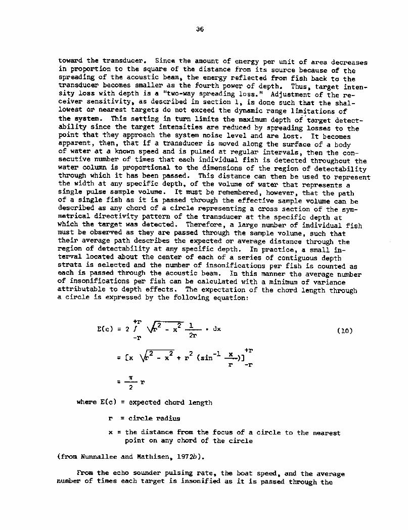
toward the transducer. Since the amount of energy per unit of area decreasesin proportion to the square of the distance from its source because of thespreading of the acoustic beam, the energy reflected from fish back to thetransducer becomes smaller as the fourth power of depth. Thus, target inten-sity Loss with depth is a "two-way spreading loss." Adjustment of the re-ceiver sensitivity, as described in section 1, is done such that the shal-lowest oz nearest targets do not exceed the dynamic range limitations ofthe system. This setting in turn limits the maximum depth of target detect-ability since the target intensities are reduced by spreading losses to thepoint that they approach the system noise level and are lost. It becomesapparent, then, that if a transducer is moved along the suzface of a bodyof water at a known speed and is pulsed at z'egular intervals, then the con-secutive number of times that each individual fish is detected throughout thewater column is pzoportional to the dimensions of the region of detectabilitythxough which it has been passed. This distance can then be used to representthe width at any specific depth, of the volume of water that represents asingle pulse sample volume. It must be remembered, however, that the pathof a single fish as it is passed through the effective sample volume can bedescribed as any chord of a circle representing a cross section of the sym-metrical diz'ectivity pattern of the transducer at the specific depth atwhich the target was detected. Therefore, a large number of individual fishmust be observed as they are passed through the sample volume, such thattheir avez'age path describes the expected or average distance through theregion of detectability at any specific depth. In practice, a small in-terval located about the center of each of a series of contiguous depthstrata is selected and the number of insonifications pez' fish is counted aseach is passed through the acoustic beam. In this manner the average numberof insonifications per fish can be calcuIated with a minimum of varianceattributable to depth effects. The expectation of the chord length througha cizcle is expz'essed by the following equation:

37

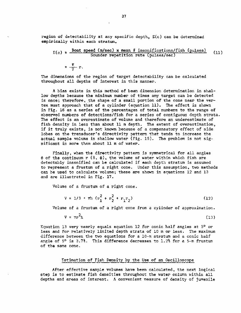
region of detectability at any specific depth, E c! can be determinedempirically within each stratum.

Boat s ed m/sec! x mean 8 insonifications/fish ulses!E c!-Sounder repetition rate pulses/sec

The dimensions of the region of target detectability can be calculatedthroughout all depths of interest in this manner.

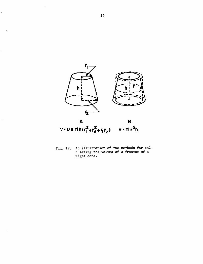
Finally, when the directivity pattern is symmetrical for all angles4 of the continuum r 8, $!, the volume of water within which fish aredetectably insonified can be calculated if each depth stratum is assumedto represent a frustum of a right cone. Under this assumption, two methodscan be used to calculate volume; these are shown in equations 12 and 13and are illustrated in Fig. 17 '

Volume of a frustum of a right cone.

V = 1/3 ' wh r + r + r r !2 2

�2!

Volume of a frustum of a right cone from a cylinder of approximation.

V = ~r h2

�3!

Equation 13 very nearly equals equation 12 for conic half angles at 5~ orless and for relatively limited depth strata of 10 m or less. The maximumdifference between the two equations for a 10-m stratum and a conic halfangle of 5 is 3.7R. This difference decreases to 1.2'4 for a 5-m frustumof the same cone.

Estimation of Fish Densit b the Use of an OsciZlosco e

After effective sample volumes have been calculated, the next logicalstep is to estimate fish densities throughout the water column within alldepths and areas of interest. A convenient measure of density of juvenile

A bias exists in this method of beam dimension determination in shal-

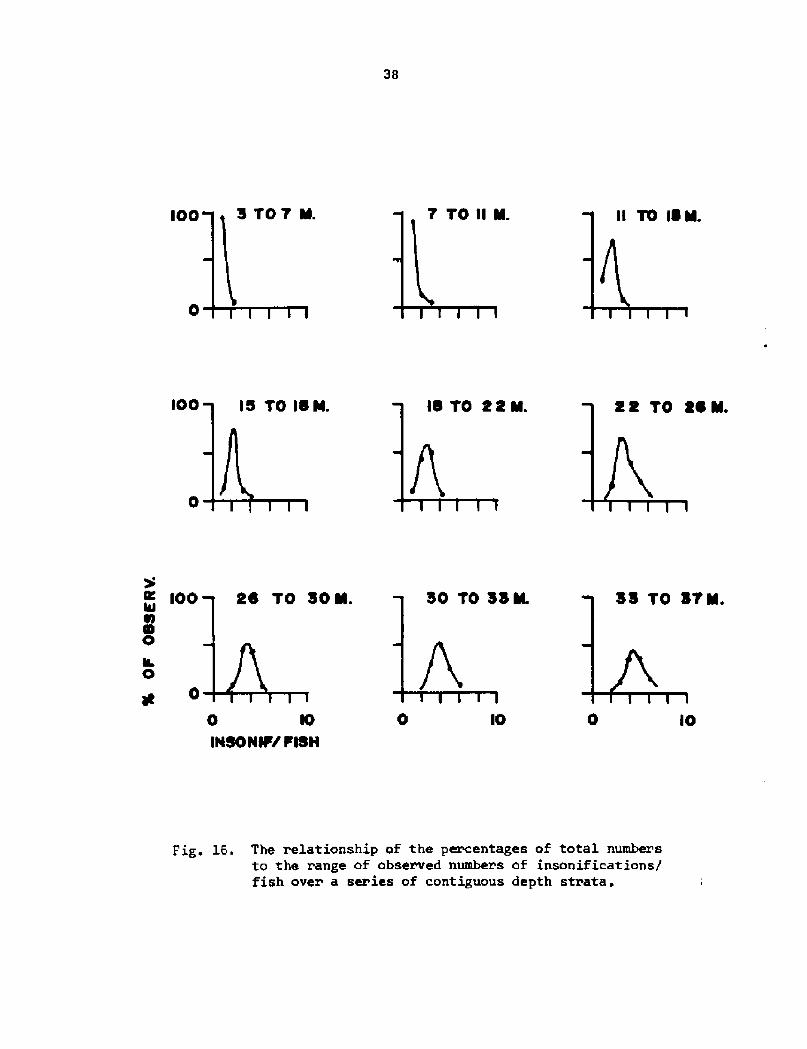
low depths because the minimum number of times any target can be detectedis once; therefore, the shape of a small portion of the cone near the ver-tex must approach that of a cylinder equation ll!. The effect is shownin Fig. 16 as a series of the percentages of total numbers to the range ofobserved numbers of detections/fish for a series of contiguous depth strata.The effect is an overestimate of volume and therefore an underestimate of

fish density in less than about ll m depth. The extent of overestimation,if it truly exists, is not known because of a compensatory effect of sidelobes on the transducer's directivity pattern that tends to increase theactual sample volume in shallow water Fig. 15!. The problem is not sig-nificant in more than about 11 m of water.

38

IOO

100

< IOO

O

g 0

OM.

0 IO

INSOHIF/ FISH

IO

Fig. l6. The relationship of the percentages of total numbersto the range of observed numbers of insonifications/fish over a series of contiguous depth strata.

39

Fig. 17. An illustration of two methods for cal-culating the volume of a frustum of aright cone.

A

v ir3tfg , ~r ~r<y~~2 2

B

Velar h

40

3salmon is in terms of fish/1,000 m . It has been found that this measuremost often falls between 1 and 50, although a few observations will be ofmuch higher and lower densities.

Two methods have been developed for the estimation of fish densities'The first method requires the use of an oscilloscope and a tape player, andthe second method includes the use of the DDAU computer. The computer methodof fish density estimation will be discussed later.

In the first case the signal channel output of the player is connectedto the oscilloscope vertical input connector and the synchronization pulseoutput is applied to the external synchronization input connector. In thismanner, the echo train from each transmitted pulse can be displayed over thewidth of the oscilloscope screen with the transmitted pulse occurring to theleft side and the bottom echo occurring to the right Fig. 4, Test point 5!.The upper and lower limits of each depth interval can be interpolated directlyfrom the oscilloscope display by measurement of the time delay of any targetdetection after the transmitted pulse from which it was originated, sincethe velocity of the propagation of sound through water is l.37 ms/sonar meter.All targets that occur within that specific stratum can be counted. In mostcases, a sweep duration of 100 ms is necessary in order that the oscilloscopecan display recordings of the entire water column, In this case, a 5-mdepth stratum �.8 ms! would be displayed within 0.68 divisions on thescreen. However, most oscilloscopes are equipped with a sweep magnifierfunction, which simplifies target counting. The sweep magnifier functionincreases the Length of the trace about the center of the screen by afactor of 10. As an example, assume a 10-ms depth stratum �.3 m! is lo-cated between 30 and 40 ms �2 to 29 m! in the water column and the sweepspeed of the oscilloscope is set to 10 ms/division. In this case, a 10-msdepth stratum can be expanded to fill the entire width of the oscilloscopescreen if the point corresponding to the mid-depth of the stratum �5 msafter the transmitted pulse! is positioned exactly to the center. The fishare enumerated by displaying each depth stratum on the oscilloscope individu-ally and by counting the total number of target detections within each fora specific number of transmitted pulses. The number of pulses and the sizeof each depth stratum are arbitrary and are most often determined by the datarequirements of the experiment.

The number of fish detected by each pulse can be treated as an indepen-dent measure of fish density, and by extension, the average density of fishwithin a larger volume can be found by dividing the total number of fish de-tections in each depth stratum by the product of the corresponding effectivestratum pulse volume and the total number of sonic !ransmissions or pings.It is easy to calculate the density of fish/1,000 m by use of the followingequat ion:

�,000! Total detections in stratum i!�4!effective pulse volume stratum i number of pings!

from Nunnallee and Mathisen, L972b!.

3The number of fish/1,000 m observed in each depth stratum can be convertedto the number of fish/l00 m2 surface area of each or of the lake surfaceby the following equation'.

n D � DLe ui

3area = Z fish/1,000 m !,i=1 10

Fish/100 m surface2

where D and D = lower and upper depth limits of stratum i respec-L. u.

i i

tively, and

n = number of depth strata.

The methods described to this point for the estimation of fish densi-ties and the numbers of fish/unit area are rather straightforward but arealso very time-consuming and tedious. As an example assume that a S-minsection of tape is to be analyzed over eight depth strata. In this case,each depth stratum would have to be displayed on an oscilloscope and thetargets be counted. The actual counting time required would be about 40 minplus the setup time required for each stratum of counts. A much improvedmethod has been developed for the estimation of fish densities that re-quires a minimum of manual target counting. This method utilizes the DDAUcomputer and hardware developed specifically for the estimation of fish den-sities. A description of the method is given in the following section.

Estimation of Fish Densit b Echo Inte ation

The second method utilizes the DDAU computer and hardware developedspecifically for the estimation of fish densities. The accuracy of the con-version of the integrated voltages in each of the memory cells to absolutedensities of fish/unit volume is proportional to the accuracy of two pro-gram parameters, A and B. These parameters include the absolute values ofmean target strength of the fish to be surveyed, the directivity functionof the acoustic energy propagated from the transducer, the sensitivity ofthe receiver including the TVG, the loss of energy due to absorption ofacoustic energy by the water and various other physical parameters.

2The number of fish/100 m surface area of a depth stratum, since it is

the proportion of a cube 10 m on a side represented by the density offish/1,000 m3, is a direct measure of the number of fish within a stratum ofany depth under an area of 100 m2. Since this measure is of the absolutenumber rather than the density of fish, the value for each stratum within awater column is additive and the sum of all values for the overall intervalis equal to the number of fish/100 m2 of the lake surface area equation 12!.Expansion of these values over a large surface area, when adequate statisticalprocedures have been applied, can yield a population estimate of the fishwithin the area.

42

Three methods can be used. to convert integrated voltages to absolutefish densities: �! to regress oscilloscope density estimates on DDAUrelative density estimates for a series oF observations and then to applythe regression coefficients to the remaining DDAU density estimates for theremainder of a survey series; �! to estimate the values of A and B neces-sary for fish density calculation; or �! to calculate the true value of Aand B for the calculation of fish density.

A FORTRAN program has been written by which the regression coefficientscan be applied to the relative DDAU values and absolute densities be cal-culated Roger, 1972!. The output of the program lists the data in twoforms. The first form is a table of fish densities/100 m2 surface area foreach of a maximum of 20 depth strata and for the lake surface. The secondform is a table of fish densities/1,000 m3 for all depth strata. A maxi-mum of four runs or transect sections can be tabulated on each page of

outputs

The usual procedure for estimating the relative abundance of juvenilesockeye salmon has been to integrate the magnetic tape recordings from asurvey series at some fixed DDAU signal gain and A and B parameter values.After this step has been completed, linear regression methods can beused to estimate the relationship of fish density estimates from oscillo-scope counting to relative DDAU density outputs for identical depth-timecells over a number of selected transects or runs. Before this method can

be used, the effects of spreading losses due to distance on echo intensityand echo integration must be considered. When acoustic energy is propa-gated through water, the wavefronts expand with the velocity of sound andtheir area increases as the square of their distance from the source',therefore, the intensity of the sound must decrease in proportion to dis-tance From the source. Intensity is given hy the expression

1 a2dc R

where I = acoustic intensity,

d = water density,

c = velocity of sound in water,

a = area of the wavefront, and

R = distance.

1t can be seen from these relationships that as the intensity of fishechoes decrease with distance, the area of the wavefront of the reflectedacoustic pulse increases proportionally. Therefore, if it is assumed thatthe fish targets are all of equal size and are randomly distributed through-out the water mass, then the sum of squared echo voltages from any stratum

Gain dB! = 20 log R,

where gain " -receiver gain dB! at the time delay after the trans-mitted pulse representing depth R, and

R = depth.

Because the oscilloscope counting threshold was necessarily equal to andopposite of the sounder TVG function, the following equation was used todescribe its shape:

R

Thzeshold level dB! = 20 log 0 " !R,

l8!

The threshold cuzve was referenced. to a level just greater than theambient system noise at the deepest depth of interest by reading the noiseamplitude on an oscilloscope and proceeding as follows using hypotheticalvalues!:

!et d = 50m, andRGX

let noise level = 45 mv;

therefore, let threshold level at 50 m = 50 mv.

R

Then, threshold dB! // 50 mv = 20 log !R.

3.

and threshold = 4.4 dB at 30 rn = 83 mv,

= 7.8 dB at 20 m = 123 mv,

= l4.0 dB at l0 m = 250 rnv.

of the water column must be the same since the number of fish detections inany stratum is proportional to depth. In brief, the echo intensity of atarget is invez'sely proportional to depth, but the number of target detec-tions per pulse is directly proportional to depth. Since the two effectsare equal but opposite, they cancel. When constant values of B are usedfor all depth strata as in the zegression method described above, an oscil-loscope counting threshold equal to, but opposite of the TVG time variedgain! function in the receiver must be used since increasing gain withdepth TVG! destroys the echo intensity-wavefront area relationship. Anidealized TVG function of the echo sounder receiver used in the researchrepresented by this report can be described by the following equation:

In this manner a series of points describing the threshold level at anydepth can be generated and plotted on an overlay of the calibrated oscil-loscope screen,

When the counting threshold described above is used, the fish densityestimates derived by counting are usually much reduced at the shallowerdepths. This occurs when small fish or other organisms are present whosetarget strengths are small enough that they are undetectable in deeperlayers. Therefore, since the threshold curve describes the change inamplitude of some minimum target strength from the surface to its maximumdepth of detectability, the small target amplitudes that fall below thethreshold and represent very low echo integration values are disregarded.The use of a counting threshold has in practice significantly reducedvariances associated with the regression method mentioned previously.

A second method, one by which the DDAU can be programmed to outputabsolute densities directly, is to proceed as above with a linear regres-sion and then to calculate values of B for each depth stratum within aseries of runs. The equation that can be used for the calculation of Bby iteration is as follows:

p = I/ ABP!, �9!

where p = fish density unit volume,

I = integrated voltage,

A and B = program parameters described previously, and

P = the number of transmitted pings over which I is derived.

When the value of p is estimated for any value of I by use of the re-gression equation, equation 19 can be solved in terms of B. The value ofA in this case can be any constant. The values af p and I are given oneach DDAU output. The value of B should be calculated for a number of runsand for each depth stratum so that the effects of variance associated withthe regression equation can be minimized by the use of mean values. Whenthese mean values are substituted into equation 19 and a B value is calcu-lated for each depth stratum, the density calculations printed at the endof each run, when these new parameters are used, wi11 be absolute densityvalue estimates for which confidence limits can be determined. When thissecond method is applied, the same counting threshold as described for thefirst method should be used. This method of determining absolute fish den-sity is superior to the first in that stratification of fish by size in thewater column will not bias the estimate to any degree if relatively narrowdepth strata are defined. It must be assumed that size distributions of thefish within the depth strata do not change during the period of the survey,however. Size stratification of the fish does not bias the estimate in this

case since the integrated voltage per fish, an indirect measure of targetstrength, is a component of the values used to calculate each B. Therefore,if the fish are larger, I will be larger, 8 will be larger, and p will beabsolute equation l9!.

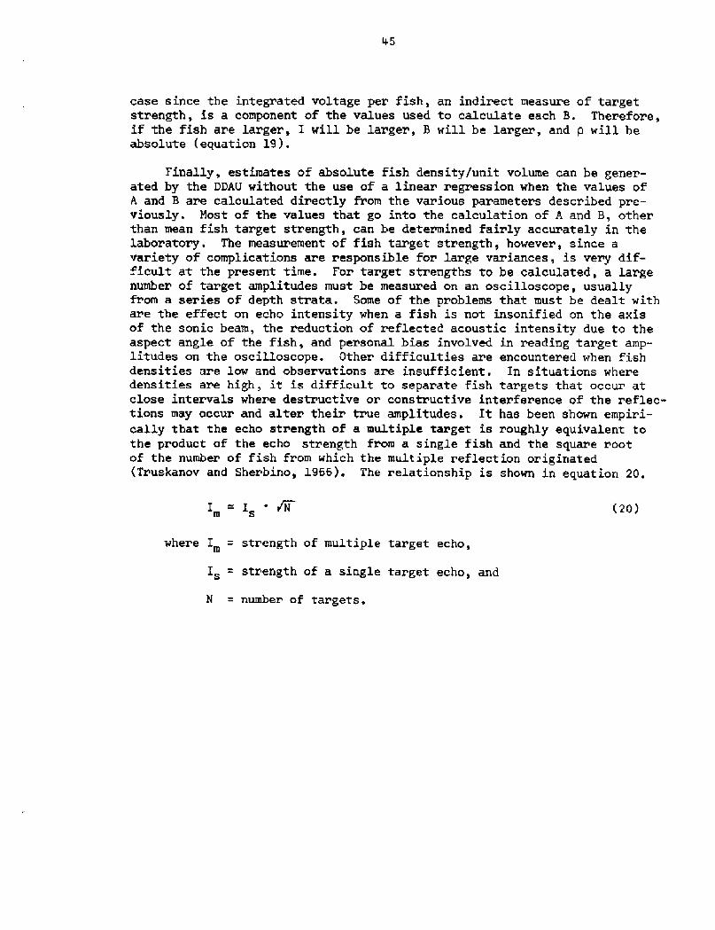
I = I ' vNm s �0!

where I = strength of multiple target echo,

Is = strength of a single target echo, and

N = number of targets.

Finally, estimates of absolute fish density/unit volume can be gener-ated by the DDAU without the use of a linear regression when the values ofA and 3 are calculated directly from the various parameters described pre-viously. Most of the values that go into the calculation of A and B, otherthan mean fish target strength, can be determined fairly accurately in thelaboratory. The measurement of fish target strength, however, since avariety of complications are responsible for large variances, is very dif-ficult at the present time. For target strengths to be calculated, a largenumber of target amplitudes must be measured on an oscilloscope, usuallyfrom a series of depth strata. Some of the problems that must be dealt withare the effect on echo intensity when a fish is not insonified on the axisof the sonic beam, the reduction of reflected acoustic intensity due to theaspect angle of the fish, and personal bias involved in reading target amp-litudes on the oscilloscope. Other difficulties are encountered when fishdensities are low and observations are insufficient. In situations wheredensities are high, it is difficult to separate fish targets that occur atclose intervals where destructive or constructive interference of the reflec-tions may occur and alter their true amplitudes. It has been shown empiri-cally that the echo strength of a multiple target is roughly equivalent tothe product of the echo strength from a single fish and the square rootof the number of fish from which the multiple reflection originated Truskanov and Sherbino, l966!. The relationship is shown in equation 20.

46

LITERATURE CITED

Balls, R. 1948. Herring fishing with echo meter. J. Cons. �5!:193-206.

Croker, T. R. 1973. Acoustic estimation of the density and abundance offish in Lake Quinault, Washingto~. M.S. Thesis. Univ. Washington,Seattle. 105 pp.

Cushing, D. H., F. Devoid, J. C. Narr, and H. Kristjonsson. 1952. Somemodern methods of fish detection � echo sounding, echo ranging, andaerial scouting. FAO Fish. Bull 5�-4!. 27 pp.

Dawson, J. J. 1972. Determination of seasonal distribution of juvenilesockeye salmon in Lake Washington by means of acoustics. M ~ S ~ Thesis.Univ. Washington, Seattle. 111 pp.

Dowd, R. G. 1967. An echo counting system for demersal fishes. Pages1-6 ~ FAO Conf. on Fish Behavior in Relation to Fishing Techniquesand Tactics. BB/67/E/7.

Dragesund, O., and S. Olsen. 1965. On the possibility of estimating yearclass strength by measuring echo abundance of 0-group fish. Fisk,Dir. Skr. Ser. Havunders 13 8!:47-75.

Ehrenberg, J. E. 1972. A method for extracting the fish target strengthdistribution from acoustic echoes. Univ. Washington. Dep. Elect.Eng., Seattle, Washington. 4 pp.

Ehrenberg, J. E., and D. W. Lytle. 1972. Acoustic techniques for esti-mating fish abundance. IEEE Trans. Geosci. Elect. July, 1972,GE 10�!;138 145.

Hodgson, W. C., and A. Fridriksson, eds. 1955. Report on echo soundingand asdic for fishing purposes. Rapp. Proc.-Verb. Reun. 139 Sept.!.49 pp.

Lahore, H. W., and D. W. Lytle. 1970. An echo integrator for use inthe estimation of fish populations. Univ. Washington, Coll. Fish.,Fish. Res. Inst., WSG 70-1. 38 pp.

Midttun, L. M. 1969. Physical properties of sound in water; its propa-gation and reflection from targets. Manual of methods for fishstock assessment. Part V. The use of acoustic instruments in

fish detection and fish abundance estimation. FAO, Rome, 1969.

Mitson, R. B., and R. J. Wood. 1961. An automatic method of countingfish echoes. J. Cons. 26:281-291.

Moose, P. H., J. E. Ehrenberg, and J. H. Green. 1971. Electronic syst' emand data processing techniques for estimating fish abundance. Univ.Washington, Appl. Phys. Lab., Seattle, Washington. rI pp.

Moose, P. H., R. E. Thorne, and MD 0. Nelson. 1971. Hydroacoustictechniques for fishery resource assessment. Mar. Tech. November-December 1971!: 35-37.

Nunnallee, E. P., and J. H. Green. 1970. A universal interface ampli-fier for coupling an echo sounder to a magnetic tape recorder.Univ. Washington, Seattle, Washington, Washington Sea Grant Publ.70-3. 8 pp.

Nunnallee, E. P., and 0. A. Mathisen. 1972a. Acoustic survey of ShuswapLake, British Columbia, Canada. Report to the Int. Pac. Salmon Comm.36 pp.

Nunnallee, E. P., and 0. A. Mathisen. 1972b. An acoustic survey of LakeWenatchee, Washington. Univ. Washington, Fish. Res. Inst. Circ.72-13. 12 pp.

Nunnallee, E. P., N. A. Lemberg, and 0. A. Mathisen. 1973. Acoustic surveyII of Shuswap Lake, British Columbia, Canada. Report to the Int. Pac.Salmon Comm. [Zn preparation.3

Pella, J. J. 1968. Distribution and growth of sockeye salmon fry in LakeAleknagik, Alaska, during the summer of 1962. Pages 47-111, Furtherstudies of Alaska sockeye salmon. Univ. Washington Publ. Fish.,n.s., III.

Roger, P. B. 1972. Calculations of stock size From integrated echo inten-sities, Fortran IV. Univ. Washington, Coll. Fish., Fish. Res. Inst.Fisheries Analysis Center. 5 pp.

Ross Laboratories Inc. 1968. Ross fine line depth recorders. Owner"sinstruction and service manual. Ross Labs. Inc., 3138 Fairview AvenueEast, Seattle, Washington. 30 pp.

Sony Corporation. 1964. Stereo tapecorder TC-560D. Owner's instructionmanual. 32 pp.

Sund, 0. 1935. Echo sounding in fishery research. Nature 135:935.

Thorne, R. E. 1970. Investigations into the use of an echo integrator formeasuring pelagic fish abundance. Ph.D. Thesis. Univ. Washington,Seattle. 117 pp.

48

Thorne, R. E. 1972. Hydroacoustic assessment of limnetic-feeding fishes.Pages 317-322 in J. F. Franklin, L. J. Dempster, and R. H. Waring, eds.Proceedings Research in Coniferous Forest Ecosystems--A symposium. U.S.Dep. Agr., For. Serv., Portland, Oregon.

Thorne, R. E., and H. W. Lahore. 1969. Acoustic techniques of fish popu-lation estimation with special reference to echo integration. Univ.Washington, Coll. Fish., Fish Res. inst. Circ. 69-10. 12 pp.

Thorne, R. E ~ , E. P. Nunnallee, and J. H. Green. 1972. A portable hydro-acoustic data acquisition system for fish stock assessment. Univ.Washington, Div. Mar. Res., Seattle, Washington. WSG Publ. 72-4.

Thorne, RE E., and J. C. Woodey. 1970. Stock assessment by echo integra-tion and its application to juvenile sockeye salmon in Lake Washington.Univ. Washington, Coll. Fish., Fish. Res. Inst., WSG 70-2. 30 pp.

Truskanov, M. D., and M. N. Scherbino. 1966. Determination of density offish concentration by means of hydroacoustics. I.in Russian] RybnoyeKhozyaystvo 8:38-42.