Watch This: A Taxonomy for Dynamic Data VisualizationJoseph A. Cottam∗

Indiana UniversityAndrew Lumsdaine†

Indiana UniversityChris Weaver‡

University of Oklahoma

ABSTRACT

Visualizations embody design choices about data access, data trans-formation, visual representation, and interaction. To interpret astatic visualization, a person must identify the correspondences be-tween the visual representation and the underlying data. These cor-respondences become moving targets when a visualization is dy-namic. Dynamics may be introduced in a visualization at any pointin the analysis and visualization process. For example, the dataitself may be streaming, shifting subsets may be selected, visualrepresentations may be animated, and interaction may modify pre-sentation. In this paper, we focus on the impact of dynamic data.We present a taxonomy and conceptual framework for understand-ing how data changes influence the interpretability of visual repre-sentations. Visualization techniques are organized into categoriesat various levels of abstraction. The salient characteristics of eachcategory and task suitability are discussed through examples fromthe scientific literature and popular practices. Examining the impli-cations of dynamically updating visualizations warrants attentionbecause it directly impacts the interpretability (and thus utility) ofvisualizations. The taxonomy presented provides a reference pointfor further exploration of dynamic data visualization techniques.

Keywords: Dynamic Data, Interpretation.

Index Terms: H.5.1 [Information Systems]: Information Inter-faces and Presentation—Multimedia Information Systems; I.3.6[Computing Methodologies]: Computer Graphics—Methodologiesand Techniques

1 INTRODUCTION

Dynamic visualizations—visualizations that change over time—are increasingly common. The way that a visualization actuallychanges impacts how it can be interpreted, both immediately andover time. Simple decisions, such as choosing to modify a colorscale in response to updated data, drastically change what the vi-sualization intuitively reveals. Such decisions can be the differ-ence between building insights and misleading. Understanding andcontrolling visual dynamics requires an appreciation of the originand manifestation of underlying data dynamics [22]. This paperpresents a taxonomy of dynamic visualization techniques.

Simply put, “dynamics” are changes over time. In the pipeline ofthe information visualization reference model [12] , dynamics canarise at any stage (see Figure 1). User interaction for navigationor to build dynamic queries are two of the most common sourcesof dynamics in visualization tools. However, the underlying dataitself may change as well. These changes may be in response toan external event, such as a sensor update, resulting in streamingupdates. Changes may also be in response to modified requirementsof the visualization with entirely new data sources seen as relevant.

When a visualization changes, regardless of the reason, thatchange must be considered in its interpretation. Choosing how the

∗jcottam@indiana.edu†lums@osl.iu.edu‡weaver@cs.ou.edu

Visual Abstraction

DataTransforms

VisualMappings

ViewTransforms

Data Tables

Source Data Views

Reference ModelDynamics

Streaming

RemappingAnimation/Navigation

Dynamic QueryUpdated Hypothesis

Figure 1: Information visualization reference model [12] andsources of dynamics at each stage.

visualization changes (i.e., in what way a visualization is dynamic)is an important part of the overall visualization design.

Visualization dynamics is too broad a topic to address as a singleunit. Important differences are found between user-driven and data-driven changes. This paper focuses on dynamic data, specificallythe effects of streaming data on a visualization. Streaming data isimportant (1) because it is growing in prevalence, (2) because datachanges are part of the InfoVis Reference Model, and (3) becauseit affects techniques further down the pipeline.

Bertin’s description of visualization techniques decomposes thevisual space into two groups: Spatial and Retinal variables [9].Spatial variables determine positions, while retinal variables coverthe other visual aspects.‘ Spatial and retinal variables are the basicbuilding blocks of data visualization. Data is encoded using thesevariables. Dynamic visualizations change over time by modifyingthe values of these variables.

Our taxonomy organizes the dynamics possible in a streaming-data visualization into four retinal and four spatial categories (Sec-tion 2). This organization is the basis for the presented taxonomy ofdynamic visualizations (Section 3). A useful description of the roleof element identity directly results from the retinal and spatial dis-cussion (Section 4). Guidelines for selecting a dynamic represen-tation (Section 5) and discussion of several existing visualizations(Section 6) are also provided.

2 TAXONOMY DIMENSIONS

Prior on classifying static visualizations provides a foundation forclassifying time-varying, dynamic visualizations. This taxonomydecomposes visualizations using distinctions made by Bertin: spa-tial and retinal variables [9]. The spatial variables are the coordi-nates in space: X and Y for two-dimensional visualizations. Retinalvariables are the size, value, orientation, texture, hue and shape of avisual element. Unlike Bertin, the taxonomy presented in this paperis not concerned with the individual properties in either dimension.Instead, it examines how these variations can be presented withineach group and the implications of different variation styles.

2.1 Spatial Variable Treatments

Spatial dimensions describe the position of an element. Positionand quantity are intrinsically related because all visual elementsmust have a position. The fundamental positional information con-sists of the X and Y position; Z position is a direct extension thatcan be applied as needed (e.g., for layering). Positional informationis considered relative to a canonical “registration point,” not regard-

193

IEEE Conference on Visual Analytics Science and Technology 2012October 14 - 19, Seattle, WA, USA 978-1-4673-4753-2/12/$31.00 ©2012 IEEE

ing the entire extent of the element (which is further influenced bysize and rotation, see Section 2.4).

Spatial dimension may be dynamic in two ways: changing exist-ing values and changing the number of visual elements (adding ordeleting). These two general change types can be expressed as fourgeneral categories:

Fixed: The spatial dimensions do not change. The number of vi-sual elements is fixed at the start of the visualization. Visualelements do not move.

Mutable: The number of elements remains fixed throughout thevisualization process, but the location of elements may changeover time. (Destructive updates are referred to as “mutation”of that entity.)

Create: New elements may be created in response to incomingdata. Existing element positions may be mutated.

Create & Delete: Elements may be created or deleted in responseto incoming data. Mutability is implicit in this category be-cause CREATE & DELETE can be used to simulate mutationto retinal attributes.

Mutation of spatial position generally falls into two styles. Bothstyles of mutation can cause significant spatial changes over timebut are not significant at the level of abstraction of this taxonomy.However, a detailed investigation of any given visualization maybenefit from noting the degree to which each case applies becausethey represent different types of relationships. The first style is achange to reflect a changing context. This style is common whenthe spatial information is not directly tied to underlying data, suchas graph layout. When the context changes, visual elements movebut that does not imply a change to the related data, only the con-text. The second style of spatial mutation occurs when spatial posi-tions are directly tied to underlying data. In this case, entity move-ment directly reflects data changes tied to the given element. Moststatistical graphics employ spatial layouts of the second type, andthus have movement dynamics in this second category.

2.2 Retinal Variable TreatmentsBertin’s retinal dimensions are size, value (light vs. dark), orienta-tion (or rotation), texture (or patterning), hue (or color), and shape.Retinal dimensions do not affect the number of individual elements(as position does), but they can affect how elements are perceivedto group. Retinal values change over time as the attribute they areassociated with do. The user of a visualization employing retinalencoding must interpret the degree of change as a correspondingvalue change. Depending on how much change is permitted, thecomplexity of this interpretation changes. The categories of retinaldimension dynamics, in increasing order of complexity, are:

Immutable: Retinal variables are set and left unchanged.

Known Scale: The scale is fixed, but future data may change theretinal presentation of an existing elements. The known scaleimplies that all values that may be presented are covered bythe scale’s regular divisions, which are established when thevisualization is initialized. For categorical encodings, knownscale means that the number and order of categories is knownin advance. For continuous encodings, the range of values isprovided in advance and divided into regular intervals.

Extreme Bin: An extreme bins scale is a known scale with sen-tinel categories (usually at the endpoints). These sentinel cat-egories may be due to an unknown actual extent of values,special/sentinel categories, or to provide details in a specificsub-range. Values outside of the regular range are assigned to

a top or bottom catch-all “bin.” Scales like this are typicallyinclude labels such as “100+”, “less than 0”, “No Data” or”Error”. These open-ended categories are distinguished andoutside of the normal divisions of the scale.

Mutable Scale: Updates may change the representation of an ele-ment and the mapping function itself. In this category, scalesmay grow or shrink dynamically to accommodate the data be-ing visualized. For example, this category may apply if thenumber of levels in a categorical variable is not known in ad-vance. When modifying scales, a single new data point maycause existing visual elements to change representations, eventhough the underlying data did not change.

Retinal dimensions are closely related to gestalt principals [44],and thus do not include symbolic meaning. This distinction indi-cates that letters, words, geographic outlines of countries, etc. arenot visual elements in-and-of themselves. Interpreting words or el-ements “from the real world” depends strongly on cultural context.In contrast, the ability to recognize variation in retinal variables isless influenced by cultural context [44]. Retinal dimensions haveinherent bandwidth. Appropriate limitations are assumed to remainconstant in the face of incremental updates and assumed to be re-spected in the visualization.

2.3 IdentityComparison is a fundamental task of visualization interpretation [1,9,41]. However, a visualization that includes dynamics complicatesthe task of comparison by inviting comparisons to be made acrosstime. This taxonomy examines how dynamics influence the taskof comparison over time. Identity can be constructed in spatial orretinal variables or in combinations of the two.

Comparisons in dynamic visualizations can be divided into tworough categories: identity based and nonidentity based. Identity-based comparisons rely on the ability to recognize an element asrepresenting the same real-world entity at multiple times. For ex-ample, in a social network, identity based comparisons require theability to recognize that a given node represents the same personas the visualization changes. Identities may be low-level (e.g., rec-ognizing individual people) or high-level (e.g., recognizing largegroups of people that live in the same state). High-level identity isreferred to as “group identity.”

Dynamics in a visualization make identity potentially fragile.The more an element changes, and the more that change happensin characteristics with strong visual salience, the more care must betaken if identity must be preserved. Identity preservation can occurat different time scales. In general, identity preservation enablesdetailed comparisons both within and between different time steps.Long-term identity preservation enables comparisons at arbitrarytime differences. However, short-term identity preservation can beused to communicate incremental changes.

Non-identity based comparisons do not enable the fine-grainedobservations that identity-based comparisons do. However, they doallow observations of distributions (within time steps) and obser-vation of distributional changes (between time steps). Non-identitybased comparisons have fewer time-scale issues [42], so small andlarge time changes affect interpretation less.

2.4 Special ConsiderationsBecause the taxonomy is focused on the influence of dynamic data,data-derived visual attributes are the principal consideration. Non-data derived attributes are assumed to be constant in this taxonomy.Since any change to the representation can introduce interpretationissues comparable to those driven by data, it is important to notethat this assumption is not strictly true. Two major circumstancesgenerally introduce changes to non-data derived attributes: graphicdesign considerations and user interaction. Changes predicated on

194

0 100

50

0 10050

Radial Linear

Figure 2: Linear and radial meters with registrations points marked.

graphic design considerations, such as resizing text to avoid over-lapping labels, can introduce interpretation issues comparable tothose driven by data. However, such events are relatively rare andthus not considered significant in this taxonomy. If the taxonomyfocused on interaction or remapping (see Figure 1), such changeswould be more significant.

Registration and transparency introduce ambiguities with respectto quantity and position. Treating visual elements as if they were onexact points is an abstraction. Visual elements have spatial extentand therefore contain more than one X/Y position. The canoni-cal position of the visual element is called its “registration point.”Rotation and size changes may induce a motion-like effect withoutchanging the registration point. The difference between radial andlinear meters illustrates this difference (see Figure 2). The pointeron a radial meter maintains a fixed registration point, though valuechanges drive rotation and thus extent changes. In contrast, valuechanges shown on a linear meter drive changes to the registrationpoint itself. Our taxonomy only considers changes to the registra-tion point as spatial changes. Extent changes are treated as retinalvariable changes.

Treatment of transparency depends on the eventual visibility. Ifthe element is always visible, transparency change is treated as aretinal variable change. However, if the visual element is madefully transparent, then it is treated as element deletion.

User interaction is a complex issue and generally deferred to fu-ture work (see Section 8). The core difficulty with user interactionis that changes in response to user actions are typically semanti-cally distinct from those in response to source data. On the surface,a user can be treated as any other dynamic data source. User in-duced changes are no more nor less extensive than data-inducedchanges. However, the user induced changes imply a shifting men-tal state in advance of the visualization and an intentional connec-tion to the change. These are the opposite conditions to those foundfrom other data source dynamics. The distinct connection betweenuser interaction and interpretation means that this taxonomy is lessapplicable to such changes than to data-driven dynamics.

Different retinal dimensions have different properties, but thistaxonomy aggregates all retinal dimensions. This simplification fo-cuses the taxonomy on issues above the level of individual retinaldimension variation. It is considered safe because variation be-tween retinal dimensions is generally of degree and not of kind.For example, eight colors is a practical maximum to use in manycontexts, despite a theoretical maximum of two million [11]. Sim-ilar maxima exist for other retinal dimensions [44]. Additionally,we only consider the retinal dimension with the greatest variation ifmultiple levels of variation are used in a visualization.

Many visualizations exhibit different behaviors at differentphases. Initialization commonly exhibits distinct behaviors. Whencategorizing visualizations, we focus on the behavior after initial-ization but do not make further phase distinctions.

3 TAXONOMY

Visualizations can be organized according to the dynamics presentin spatial and retinal dimensions. Four divisions of variability forboth spatial and retinal variability were identified and described indetail in Section 2. In brief, the spatial properties of a visual el-ement may be (1) fixed at the start (FIXED), (2) mutable over the

Immutable KnownScale

ExtremeBins

MutableScale

Mutate

Fixed

Create

Create &Delete

Retinal Categories

Qua

ntat

y/Sp

atia

l Ca

tego

ries

Identity Preserving

Transitional

Immediate

(a) Technique Matrix

Spatial×Retinal DescriptionF×I No dynamics present

F×KS Elements are statically positioned with dynamicretinal encodings.

F×EB Retinal encodings with details in a limited rangeof the data.

F×MS Retinal encodings where the value and the value’sscale convey dynamic information.

M×I Mobile elements with constant appearance.M×KS Elements may move and their appearance may

change in a priori known ways.M×EB Moving elements with emphasized retinal range.M×MS A fixed number of elements, but retinal encodings

and scales are dynamic.C×I Elements may be created with fixed appearance.

C×KS Created elements are always retained, but their ap-pearance may change over time.

C×EB Element creation with emphasized retinal range.C×MS Number of elements can increase, their appearance

(including the scales) change with data.CD×I The set of elements can grow or shrink, but appear-

ance is fixed.CD×KS Elements appear and disappear; existing elements

can change appearance.CD×EB Elements appear and disappear, with representa-

tion providing details within a range.CD×MS Quantity, retinal encoding, and scales can change.

(b) Technique Descriptions

Figure 3: Retinal vs. Spatial Mutability matrix and brief descriptionof technique categories. Descriptions are labeled with abbreviatedspatial and retinal categories.

course of the visualization (MUTABLE), (3) new visual elementsmay be added (CREATE) or (4) existing spatial elements may bedeleted (CREATE & DELETE). Spatial modification in options 3or 4 also changes the quantity of elements in a visualization. Fourdivisions of retinal variability were also introduced: (1) set at cre-ation time (IMMUTABLE), (2) mutable on a fully-defined and reg-ular scale (KNOWN SCALE), (3) mutable on a defined scale withdistinguished ‘bins’ (EXTREME BINS) and (4) scales may updatein response to new data (MUTABLE SCALE).

Since spatial and retinal variables are orthogonal to each other,the degrees of variability in each are also orthogonal. Combined,they define a 4-by-4 matrix of technique categories (see Figure 3).Visualizations within a technique category share identity-relatedproperties, and neighboring categories generally represent incre-mental changes to those properties. This section describes each ofthe technique categories, including examples in existing visualiza-tions and a discussion of identity properties.

195

3.1 Dynamic Technique CategoriesThe taxonomy matrix includes sixteen technique categories. Thissection provides a more detailed description of each category.

FIXED×IMMUTABLE (F×I)Visualizations that are fixed in spatial dimensions and immutable inretinal dimensions are static. This is the degenerate case of dynamicvisualization. From the standpoint of identity, visualizations of thisclass have strong identity characteristics and thus enable arbitrarycomparisons, but really only ever show one time step.

FIXED×KNOWN SCALE (F×KS)A fixed spatial representation can present a stable reference system,on which retinal dimensions indicate changing information as anoverlay. A road atlas is a static version of such a system, with roadpositions as the reference and road type (divided highway, high-way, unpaved road, etc.) as retinal annotations. A dynamic trafficmap [36] extends this idea to dynamic data: as the road congestionchanges, so does the coloring (i.e., retinal encoding) of the road seg-ment. In such maps, the road positions do not change, so identityis tied directly to position. Overlay of symbolic data in a heads-up display works in a similar fashion, but the reference system isthe real world [3]. A “map of science” can form a metaphoricalsubstrate for other data to be encoded on the retinal variables [10].Staying within a known scale for retinal variation can be achievedin post-hoc displays of historical information or using scales in ahistorically or analytically derived safe range.

FIXED×EXTREME BINS (F×EB)Combining extreme bins with a fixed reference system providesa stable presentation of potentially complex data. A temperaturemap is a common form in this category. The map coloring corre-sponds to temperature. However, when the color enters the highestor lowest bins, the only safe statement is that temperature exceededthe normal scale. FIXED×EXTREME BINS visualizations are use-ful when the entities are known (such as frequency bins in a musicequalizer or physical locations on a map) and a subset of possiblerange is interesting or common. Such visualizations may also pro-vide a focus+context effect [37]. The focus area is a sub-range ofthe input values, but the context is provided by the extreme bins.

FIXED×MUTABLE SCALE (F×MS)At any give time, visualizations in the FIXED×MUTABLE SCALEcategory appear like those in other FIXED categories. However, inthis category, the retinal scale itself changes to accommodate thedata. For example, if color used to communicate a range of values,the color of an element indicates the relative position of the value ina range and the scale communicates what that range actually is. Ingeneral, visualizations using a mutable scale must be interpreted asa composite of the value displayed and the scale it is displayed on.If value-vs-extrema (e.g., min or max) is important, this category isappropriate. However, if absolute values are important, visualiza-tions in this category may be more difficult to interpret.

MUTATE×IMMUTABLE (M×I)Visualizations employing spatial change have objects which maymove around but otherwise have fixed appearance. Visualizationsin this category are effective when the most important aspect ofcomparison naturally maps to a coordinate space, such as spatialtracking of specific entities. When used for tracking, identity is es-tablished by the retinal characteristics. This places a practical limiton the number of distinguishable elements or element categories(as was done in [16]). Visualization in this category can be used toview distributions of large quantities of elements as well (see NYTaxi cabs [34] and the Sexsperience 1000 [35]).

For visualizations where spatial mutation is possible but entitydeletion is not, a common technique is to use a distinguished lo-cation to indicate “out of selection” or ”other” (used by We FeelFine [21] and Sexsperience 1000 [35]). Having a distinguishedlocation may introduce spatial non-uniformity, (e.g., if the spatialscales are otherwise linear). This can lead to mis-interpretation ifthe distinguished location is not properly labeled.

MUTATE×KNOWN SCALE (M×KS)Visualizations in this category can move elements in space andmodify their properties as they do so. Such visualizations gener-ally preserve element identities in the short-term (e.g., if spatialmovement is done slowly). However, because position and reti-nal values can change over time, long-term identity preservation isnot guaranteed. Despite the ability to change any attribute, changesare bounded to known ranges. Spatially, the quantity of elementsis fixed. Retinal presentation may only vary over pre-determinedranges. The Zugmonitor [39], as it presents the position and ex-pected delay of trains, fits in this category.

MUTATE×EXTREME BINS (M×EB)Visualizations in this category are similar to those in MU-TATE×KNOWN SCALE in that variation is bounded. However, inMUTATE×EXTREME BINS only a subset of the dynamics underly-ing the retinal variables can be represented. In some ways, visual-izations in this category focus on an interesting range whereas thosein MUTATE×KNOWN SCALE use the entire retinal space more uni-formly. MUTATE×EXTREME BINS visualizations provide details incontext, and can do so with both spatial and retinal values. How-ever, comparisons across long time spans are difficult since no ele-ment of the visualization is necessarily stable.

MUTATE×MUTABLE SCALE (M×MS)In this category, visualizations present a fixed number of entities,but may modify the retinal encoding in arbitrary ways. The tree-map stock market representation at Smart Money fits this cate-gory [8, 45]. The number of tree cells in the maps of the marketis fixed, each corresponding to an individual stock. The color ofthe cells represents percent value change. However, the color scalechanges as new data is acquired, always accommodating the largestpercentage change currently in the map. Therefore, the same highsaturation color in a cell in any given time-step may represent sub-stantially different values. MUTATE×MUTABLE SCALE visualiza-tions show detail for the current state when only a fixed number ofvisual elements are required.

CREATE×IMMUTABLE (C×I)Introducing new elements to a visualization introduces an addi-tional level of complexity. Depending on how mutability is used,visualizations in this category may or may not preserve identity.Generally, if identity is created by position then it can be preservedover short time periods, but large position changes (even cumula-tive) make long-term identity preservation unlikely. However, ifidentity is preserved via the retinal variables, it is preserved indefi-nitely. Dynamic timelines belong in this category of visualizations,such as Yanni Loukissas’s Apollo 11 visualization [25]. As timeprogresses, new elements from a variety of data sources are addedto the left-hand side of the display.

CREATE×KNOWN SCALE (C×KS)Visualizations in this category can employ element creation, posi-tional mutation and mutable appearance along a known scale. With-out fixed retinal representation, identity establishment is furthercomplicated over CREATE×IMMUTABLE. As with all categoriesin the CREATE row, judicious use of retinal and spatial mutationcounteracts these effects. Visualization in this category can be used

196

to track an increasing number of elements. For example, in TheNew York Talk Exchange [32], positional mutation is not used be-cause location is based on physical geography. In contrast, dynamicgraph layout algorithms that do not preserve context use positionalmutation extensively as new nodes are added [4, 5].

CREATE×EXTREME BINS (C×EB)As with all extreme bins visualizations, visualizations in this cat-egory enable more detailed presentation of specific ranges of val-ues. Adding the ability to create new elements introduces a newdynamic over just spatial mutability. For example, new informationcan be retinally emphasized but eventually presented more consis-tently (as is done in by Nathan Yau to show growth of the retailstores Target, Walmart, and Sam’s Club [48]). Another commonpattern in this category of visualizations is to subdue superseded orexcluded values without fully removing them. Subdued values re-main in position and provide context, but belong to a retinal ‘bin’that de-emphasizes them. Visualizations in this category can beused to represent deleted elements [5].

CREATE×MUTABLE SCALE (C×MS)In this category, visualizations tend to use a stable spatial substrate,but accumulate elements and constantly re-encode retinal variables.The Digg Arc [15] visualization belongs in this category. New ele-ments are accumulated into individual arcs, but color re-encoded aspercentages shift to different parts of the circle. When used with aslow-changing reference system (such as Digg Arc uses), this visu-alization can retain identity over short time periods. However, thisidentity preservation is not generally guaranteed. The mutable scaleand ability to add an arbitrary number of elements over time makelong-distance comparisons difficult. As a MUTABLE SCALE visual-ization, the current state shows maximal detail on retinal variables.

CREATE & DELETE×IMMUTABLE (CD×I)Visualizations that allow elements to be created and deleted (as wellas mutated) enable the tracking new elements over time without re-taining old elements. Retinal dimensions may also encode addi-tional data. Identity can be established with the retinal encoding.Despite the immutability of the retinal encoding, identity cannotbe guaranteed over long periods since elements may be removed.Visualizations in this category are suited to tracking elements oftransient interest, like HDPV does with memory objects [40].

Strictly speaking, any visualization that allows creation and dele-tion of elements can simulate mutability. An element can be re-moved and a new element instantiated with slightly modified retinalcharacteristics. The distinction between this category and CREATE& DELETE×KNOWN SCALE relies not on capability, but rather ob-served behavior. If visual elements maintain their retinal character-istics throughout their time in the visualization, they belong in theIMMUTABLE column, even though modification can be simulatedwithout violating the behavioral characteristics of this category.

CREATE & DELETE×KNOWN SCALE (CD×KS)Visualizations in this category behave much like those in CREATE& DELETE×IMMUTABLE. However, in this category retinal rep-resentation of individual elements can also change. Such changesdecrease the ability to make identity-based comparisons, but facil-itate greater flexibility to represent shifting categorizations of val-ues. Techniques in this category can include fading values out overtime [7] and radar-like tracking [6].

CREATE & DELETE×EXTREME BINS (CD×EB)In this category, elements can be created and deleted, with tran-sient information displayed in retinal variation. Extreme bins allowa specific data range to be highlighted. These techniques are usedin Wattenburg’s wind-speed visualization [46], and NASA’s ocean

current diagram [28]. Related techniques are used to represent thestock market via Boids [27]. In all of these cases, the flow is anemergent property of many small motions and supplemental infor-mation is overlaid in the flow. Comparisons in short time-stepsfocus on group trends in position, overlay values or both. Visu-alizations in this category have very weak identity properties forindividual elements, though group identity may be present.

CREATE & DELETE×MUTABLE SCALE (CD×MS)This final category of visualization techniques can present thecurrent data state with the highest degree of fidelity. How-ever, it is the weakest for comparisons across time. Much likeFIXED×IMMUTABLE visualizations, comparisons are restricted towhat is presented at any given instant. However, in CREATE& DELETE×MUTABLE SCALE visualizations, the visualizationchanges over time, inviting comparison. Such comparisons mustbe made carefully, as changing scales reduce the ability to recogniz-ably encode group identities. Despite this restriction, visualizationin this category can communicate step-by-step changes in a com-plex space. Short term comparisons can be made when changes aremade slowly and vary a small number of elements at once (this isfurther helped by following animation guidelines [18]).

4 HIGHER-LEVEL CATEGORY: IDENTITY GROUPS

Identity properties form three groups from the techniques presentedin Section 3. The three identity groups, in decreasing order ofidentity preservation, are: Preserving, Transitional and Immediate.These groups are formed from the interplay between spatial andretinal categories. The identity groups are an emergent structurein this taxonomy. They have implications for the pervasive task ofcomparison through time [5, 18, 42].

PreservingPreserving techniques maintain the association between visual ele-ments and underlying data across arbitrary time scales. This preser-vation of identity is achieved by holding some part of the represen-tation of an element constant. Fixed locations preserve identity infour of the techniques groups in this category. Position is of highvisual salience, and thus the identity association is strong and easyto decode. In contrast, visualizations in the MUTATE×IMMUTABLEcategory keep the retinal encoding constant, while permitting po-sition to change. This allows greater expressiveness in the spatialdimension, but increases the cognitive load for fine-grained com-parisons (though they remain possible). Preserving techniques donot require additional effort for identity preservation; it is inher-ent in the bounds on dynamics. Preserving techniques can repre-sent a great deal of dynamic information. They are most easilyachieved when the range of dynamic inputs are known. Preservingtechniques are essential when comparisons need to be made overlong periods of time.

TransitionalTransitional techniques often retain identity associations, but theassociation is not as strong as for Preserving techniques. Transi-tional techniques retain identity associations across time by limitingchanges to only known values. From the standpoint of quantity, newelements may be added or changed (but not both if long-term iden-tity is needed). Retinal encodings are also bounded. Transitionaltechniques preserve identity association over short time scales with-out difficulty. However, each technique category has at least oneway that identity associations can be destroyed by design decisions.Transitional techniques balance encoding flexibility with detailedcomparison across time. Fine-grained comparison is easily sup-ported over short time spans, but degrades over longer spans. Theyprovide greater degrees of freedom for presenting and contextual-izing current information than Preserving techniques.

197

Identity Preserving

Transitional

Immediate

Should comparisons be prioritized across or in the current time?

Start

Current state

Time comparison

Is there temporal variation in supplemental data?

Yes

No

Unknown

NoneKnown

Unknown

NoneKnown

Yes

No

Unknown

NoneKnown

Unknown

NoneKnown Mutate

Fixed

Create

Create &Delete

Immutable KnownScale

ExtremeBins

MutableScale

Is there a stable reference system?

Figure 4: Decision tree for mapping from specific tasks to a techniques through the taxonomy.

The CREATE×IMMUTABLE technique category is the only IM-MUTABLE Transitional category. The inclusion of spatial mutationin CREATE visualizations makes this category transitional. Unlessthe retinal characteristics are specifically used to encode identity,identity is difficult to establish across time. New elements and mov-ing old elements quickly degrade identity characteristics.

ImmediateImmediate techniques may retain identity associations, but onlythrough careful design choices. Those design choices also fall out-side the scope of this taxonomy (such as varying one visual dimen-sion widely but fixing another, see Section 2.4). By default, Imme-diate techniques do not preserve the identity association. In the caseof categories in the CREATE & DELETE row, identity is destroyedwhenever an element is removed from the visualization. For visu-alizations in categories of the MUTABLE SCALE column, identityis destroyed whenever a retinal scale is remapped. This identityassociation destruction may prevent comparisons over short time-scales as well as long time scales. (Removed items cannot be foundand remapped color scales cannot be compared in subsequent timesteps, even if there is only one time step between the two images).

Immediate techniques are valuable techniques, despite limitedidentity preservation. They provide the detailed information in themost flexible format right now. They are poor for making compar-isons across time steps.

5 TASK TO TECHNIQUE MATCHING

The Preserving, Transitional and Immediate identity groups pre-sented in Section 4 are central to effectively applying this taxon-omy to new visualization problems. A common task is to have adynamic-data visualization problem, and to need a technique to fitthe problem. Since not all techniques enable the same kinds ofcomparisons, selection is a process of matching project priorities totechnique capabilities. Once a suitable technique category is identi-fied, neighboring techniques can also be considered because neigh-bors in the taxonomy hold similar characteristics. Changes fromone technique category to a neighboring technique category are in-cremental but cumulative (therefore, diagonal neighbors are twosignificant changes away). The process of selection can be pursuedin three questions: (1) “Should comparisons be prioritized across

time or in the current time?”, (2) “Is there a stable reference sys-tem?” and (3) “Is there temporal variation in supplemental data?”Answers to theses questions select an identity group, a spatial tech-nique category, and a retinal row. This mixture of task and data-typequestions is not uncommon in visualization taxonomies (for exam-ple [1, 37, 47]). Practically, the questions may be answered in anyorder convenient. These questions, and the suggestions offered inthis section based on their responses, are derived from Gestalt prin-cipals [44] and supported by pre-existing evaluations of techniquespresented by others. Figure 4 illustrates the process.

The initial question of the decision tree is: “Should comparisonsbe prioritized across time or in the current time?” Selecting the de-sired characteristics of comparison determines identity preservationproperties. If comparisons across a large amount of time are re-quired, then (identity) Preserving techniques are preferable. Pre-serving techniques retain a strong sense of context over time. Con-text construction and preservation improves interpretation of analy-sis for questions that rely on it [4]. In contrast, if only the immediatecontext is required, visualizations from the Immediate categoriespresent this context with increased fidelity. Transitional techniquesmay be adapted to either circumstance, but are so categorized be-cause they preserve short-term context. Short-term context can beused for analysis tasks where long-term context is not required [7].

“Is there a stable reference system?” is the second question. Areference system is composed of the quantity of elements combinedwith some task-significant relationship between them. Geographyand slow/unchanging social relationships can be used as stable ref-erence systems [1,10]. If a reference system exists and it is relevantto the task, then representing it improves analysis performance [5].Visualizations commonly represent reference systems via spatialencoding [10]. Spatial techniques in the upper taxonomy rows re-tain spatial reference systems more than those lower in the matrix.If a reference system is not applicable, the lower parts of the matrixyield more representational flexibility.

The final question is: “Is there temporal variation in supplemen-tal data?” This question clarifies the role of data supplementingwhich supplements the data used in spatial encoding. The sup-plemental data is encoded in retinal variables. “None”, “Known”and, “Unknown” are the possible answers to this question. Theseresponses map directly on to columns in the matrix.

198

In general, using a technique from a neighboring category willyield similar results because encoding and identity properties aresimilar. For example, the EXTREME BINS column is not directlyindicated by any of the responses to the third question. It rep-resents an intermediate category between the “Known” and “Un-known” cases, and may be effective in many circumstances for ei-ther. Whether to choose the indicated column or shift to EXTREMEBINS is task-dependent. Providing more detail in a specific range isa reason to shift from KNOWN SCALE; improving long-term inter-pretability is a reason to shift from MUTABLE SCALE. In general,deciding to make such a shift may be predicated on conventions ofthe target audience, available mapping functions, additional knowl-edge about the data set or detailed task requirements.

An example application will clarify the search process. Startingwith a group of people in a social network and a set of elements theymay “up-vote”, design a visualization to address the question, “Dopeople who like the same things tend to provide new, shared up-votes around the same time?” This question is a precursor to treat-ing social behavior as an “infectious” phenomenon [20]. Since thetime-scale of comparisons is not known, we will assert (in responseto question 1) that long-distance comparisons are important. Thesocial network is not a stable substrate—membership changes, asmay member roles– providing a negative response to question two.Finally, “up-voting” an element is a binary response, so variationis “known” in supplemental data. Preferring long-distance com-parisons over an unstable substrate with known variability in sup-plemental information leads to the CREATE×KNOWN SCALE cate-gory. CREATE×IMMUTABLE may be used if up-vote quantity doesnot matter; asserting that it is only significant that an item receivedsome up-vote. If the number of items that may be voted on is fixed,a MUTATE×IMMUTABLE may be used instead, but this changes thevisualization’s focus from people to items. If the number of peopleis known in advance (changing the dynamics assumed in questiontwo), a MUTATE×IMMUTABLE technique may also be employed.

The example question above is closely related to the re-search questions underlying New York Times Labs: Project Cas-cade [29]. One Project Cascade visualization belongs to the CRE-ATE×IMMUTABLE category. In Project Cascade, nodes representevents. New events induce new nodes that are given stable loca-tions (placing it in the CREATE row). Each event is categorizedat creation time, with retinal variables representing this category.Therefore, Project Cascade essentially presents a dynamic timelineof events. Because events are created, but not generally moved,Project Cascade visualizations have higher identity preservationthan most Transitional visualizations.

6 DYNAMIC VISUALIZATION EXAMPLES

The taxonomy presented in Section 3 can be used to describe andcritique dynamic data visualizations. In this section, we have se-lected exemplar visualizations to analyze using it.

6.1 Gapminder World

(a) Default Configuration (b) Traces Enabled

Figure 5: Gapminder World’s time-dependent visualizations [17].

The Gapminder World tool [17] generates visualizations for ob-serving trends over time. In its default configuration, it presents ascatter plot of values as they progress over time (Figure 5a). Thescatter plot mutates the position of a fixed number of elements andmodifies size on a known scale as data changes. Therefore the pre-sentation mode is in the MUTATE×KNOW SCALE category. Thiscategory is consistent with the goal of enabling comparisons be-tween time steps that focus on the values selected for the axes.

Gapminder World can be configured to provide different typesof visualizations. For example, prior node positions can be retainedover time (the “traces” option), creating a visualization in the CRE-ATE×KNOWN SCALE category where no mutation is used. Thetaxonomy structure suggests that performance between traces andnon-traces would be similar, given that they belong to adjacent tax-onomy categories. Robertson, et al. confirm this hypothesis [33].

6.2 Flow Lines

Figure 6: Flow lines example taken from [43].

Flow lines represent dynamically shifting, emergent structures(Figure 6). This visualization is constructed by generating a tex-ture of discrete points in response to an input topology [43]. Asthe topology changes, so does the texture. The texture may be ani-mated to illustrate flow direction and magnitude. Flow lines presentinformation about the underlying topology through ephemeral en-tities; therefore, long-term identity preservation is not required andmay not even be desirable. In its common form, this visualiza-tion belongs to the CREATE & DELETE×KNOWN SCALE category,a member of the Immediate identity group. Textual points, the ba-sic unit of this visualization, may be created and deleted. Retinalvariables may be used to encode specific information about points.For example when using “dyes,” color communicates origin. It mayalso be used to emphasize velocity or direction (as is used in Wat-tenburg’s wind visualization [46]).

6.3 code swarmThe code swarm visualization [31] shows the shifting relationshipbetween documents and their multiple authors. It uses the positionof points (representing documents) around text labels (representingauthors) to describe the activity of a software repository (Figure 7).The labels are the only elements that preserve identity; they have aconsistent representation and move slowly. The positional informa-tion and quantity of elements are revealed dynamically as emergentproperties of developer activity. Color is used to indicate both filetype and recent activity on an EXTREME BINS scale. This is a morecomplex encoding than the KNOWN SCALE used to encode size.The net effect of the presentation decisions is to generate a sense oftrends that are composed of individual elements in the visualization,but trend membership changes over time. This presentation con-forms to the CREATE & DELETE×EXTREME BINS category. Com-

199

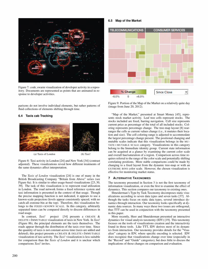
Figure 7: code swarm visualization of developer activity in a repos-itory. Documents are represented as points that are animated in re-sponse to developer activities.

parisons do not involve individual elements, but rather patterns offluid collections of elements shifting through time.

6.4 Taxis cab Tracking

(a) Taxis of London (b) Taxi!

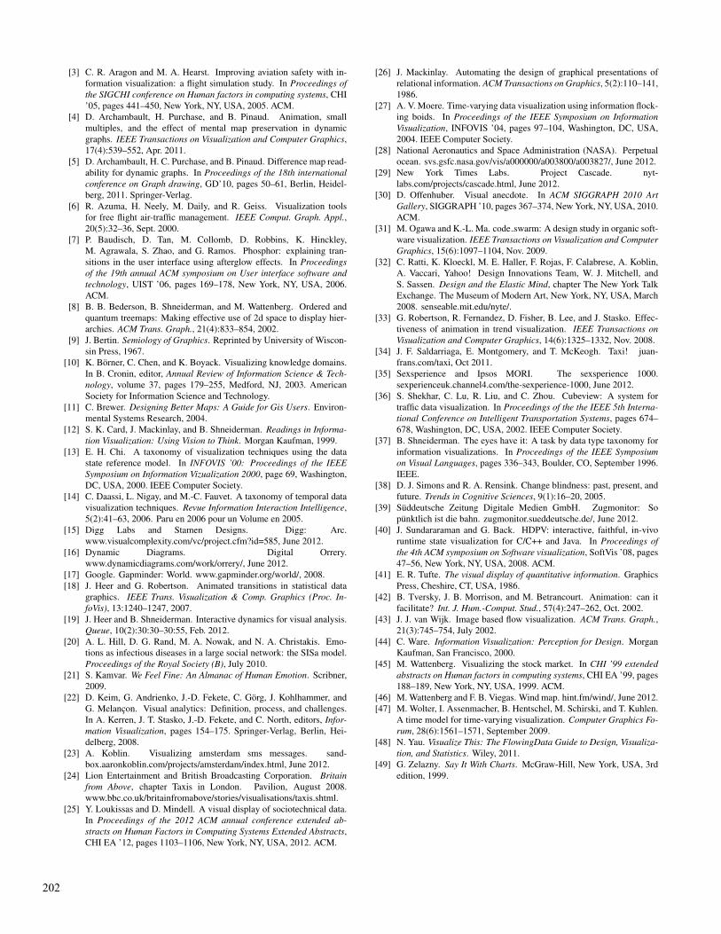
Figure 8: Taxi activity in London [24] and New York [34] (contrastadjusted). These visualizations reveal how different treatments ofthe same dynamics affect interpretation.

The Taxis of London visualization [24] is one of many in theBritish Broadcasting Company “Britain from Above” series (seeFigure 8a). It is similar to other usage-based visualizations [23, 30,39]. The task of this visualization is to represent road utilizationin London. The road network forms a fixed reference system andtaxi information is presented in the context of that usage. Thoughthe precise mapping function is not indicated, it appears to use aknown-scale projection (levels appear consistently spaced, with nocatch-all extreme-bin at the top). Therefore, this visualization be-longs to the FIXED×KNOWN SCALE. In this category, arbitrarilyseparated times can be compared directly to discern differences inroad usage.

In contrast, Taxi! project [34] presents a CREATE &DELETE×IMMUTABLE visualization of taxis in New York. In Taxi!(Figure 8b), the principal elements are the taxis themselves. Theroads appear through the distribution of the taxis over time. Sincethe quantity of taxis is not constant across time (taxis are added anddeleted), this project presents a CREATE & DELETE×IMMUTABLEvisualization of taxi activity. The Taxi! visualization is less suitablefor comparison than the Taxis of London and it is unclear whichcomparisons Taxi! invites.

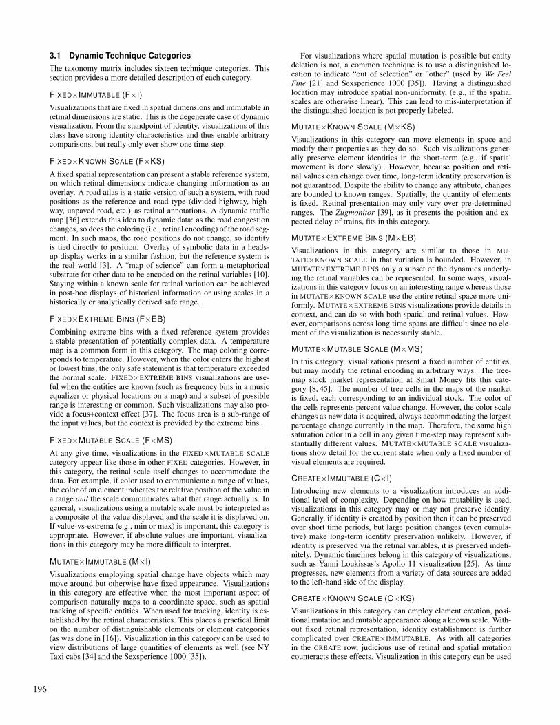
6.5 Map of the Market

Figure 9: Portion of the Map of the Market on a relatively quite day(image from June 20, 2012).

“Map of the Market,” presented at Smart Money [45], repre-sents stock market activity. Leaf tree cells represent stocks. Thestocks included are fixed, barring navigation. Cell size representscurrent price as percentage of the total of all included stocks. Col-oring represents percentage change. The tree-map layout [8] rear-ranges the cells as current values change (i.e., it mutates their loca-tion and size). The cell coloring range is adjusted to accommodatethe largest percentage change present. The positional changing andmutable scales indicate that this visualization belongs in the MU-TATE×MUTABLE SCALE category. Visualizations in this categorybelong to the Immediate identity group. Current state informationcan be acquired at a glance by examining the current color scaleand overall hue/saturation of a region. Comparison across time re-quires referral to the range of the color scale and potentially shiftingcorrelating positions. More stable comparisons could be made bychanging to a fixed layout from the dynamic tree-map or with anEXTREME BINS color scale. However, the chosen visualization iseffective for monitoring market status.

7 ALTERNATIVE TAXONOMIES

The taxonomy presented in Section 3 is not the first taxonomy ofinformation visualization, or even the first to examine the effect ofdynamics. This section compares our taxonomy to existing ones.

Shneiderman’s Type by Task Taxonomy decomposes static visu-alizations according to seven data types and seven tasks [37]. Al-though the tasks focus on static data types, several introduce dy-namics through interaction. Our taxonomy looks specifically at dy-namic data sources. In many ways these two issues are orthogonal,thus TTT can be used in conjunction with the taxonomy presentedin this paper.

More recently, Heer and Shneiderman presented an interactivedynamics for visual analysis taxonomy (IDV) [19]. This taxonomyfocuses on the tools of visualizations creation and the interactivityfound in those tools. Like TTT, IDV derives most of its dynam-ics from interaction. Our taxonomy provides details for the “Visu-alize” category in IDV, where specific encoding is selected. IDVdoes recognize that visualizations change over time (especially inthe “Record” and “Guide” categories), but does little to discuss theimplications of those changes on comparison and evaluation.

200

Heer and Robertson present a taxonomy of animation tech-niques [18]. Since data dynamics often appear as animation, theirtaxonomy provides useful context. Specifically, the spatial variationdescribed in our taxonomy provides detail to their “Substrate Trans-formation” category. Similarly, the retinal variation of our taxon-omy provides four subcategories for their “Visualization Change.”Their discussion of congruence [18,42] provides useful informationabout maintaining comparison capabilities in the face of changes toa visualization.

Keim, et al. indicate temporal data analysis as a significant areaof analytics research and a need for “...identification of patterns (...),trends and correlations of the data elements over time...” [22]. Theyfurther identify presentation selection as a significant challenge forall visual analytics processes. Our taxonomy presents a means toselect visual representations based on the the types of comparisonsdesired (Section 5), and to categorize a visualization to understandits potential weaknesses (Section 3).

Chi presented a taxonomy for describing visualization processesbased on the data-state model of visualization [13]. Chi’s taxonomydescribes the design space for data transformation by enumeratingthe different transformation stages. This taxonomy is applied byenumerating the processing performed at each stage of the infor-mation visualization pipeline (Figure 1) [12]. Chi’s taxonomy islargely agnostic to data dynamics and does not attempt to provideguidance in design. Our taxonomy treats dynamics specifically. Inaddition to being descriptive, the search procedure from Section 5aids directly in design by mapping low-level data characteristics tohigh-level properties of the visualization.

Several taxonomies of time-varying data have been presented [1,2, 14, 47]. However, most of these taxonomies assume that the datais historical, and thus static from the standpoint of analysis and vi-sualization. In the terminology of [47], there is no variation in usertime driven by changes in the data. These static, time-oriented tax-onomies focus on how analysis and representation can be used toeffectively convey historical dynamics. Our taxonomy presents aframework for discussing how changes to the visualization itselfaffect interpretation over time. These other taxonomies do provideinsight into mechanisms for effective interpretation. For example,the different options for presenting event-based analysis results pre-sented in [2] can be categorized according to our taxonomy. Theprocess described in Section 5 can assist in matching user tasks anddata characteristics to a visual representation.

Aigner, et alpresent a taxonomy for time oriented data thatspecifically includes dynamic representations [1]. However, theytreat all dynamic representations as equal and do not “...investigatethe subtle details of the variety of visual approaches available.” Ourtaxonomy addresses this omission directly for dynamic represen-tations in the same way that earlier static taxonomies do for staticrepresentations [26, 49]. In their discussion of dynamics, Aigner,et al. (supported by others [19, 38]) indicate that long-term com-parisons are often untenable due to the limits of visual memory,noting that “...the animation takes too long for users to rememberits course.” This issue is a principal disadvantage of visualizationsin the IMMEDIATE category of our taxonomy, but visualizations inthe PRESERVING and TRANSITIONAL categories (when treated ap-propriately) can present the cumulative history, eliminating muchof this cognitive loading. Access to images from prior time-stepsmay also reduce the cognitive load of comparisons across large timeranges by reducing memory effects [18, 42].

In summary, the taxonomy presented in this paper is unique inthat it provides an analysis of dynamic data representations. It pro-vides a description of eight different types of variation (four spatialand four retinal) and three higher-level categories. These categorieshave been useful in exploring the properties of existing visualiza-tions. Our taxonomy does not provide guidance about working withdifferent types of time (cyclic vs. linear, etc.) and does not pro-

vide a detailed analysis of the comparison process (only comparisonaids). It also does not provide guidance to the specific analysis toperform, only broadly restricting it based on representational prop-erties. Where many prior taxonomies investigate the entire analyti-cal process from a high-level perspective, our taxonomy focuses onrepresentation and interpretation.

8 EXTENSIONS AND CONCLUSIONS

The taxonomy presented in this paper focused on streaming data.However, the distinct characteristics of other types of dynamics arenot addressed. For example, the distinction between user-requestedand data-derived changes to the visualization is qualitatively sig-nificant but not considered. Though zoom/pan navigation can bethought of as a mutable position technique, zoom and pan do notmodify the reference system; instead, they modify the viewport ontothat reference system. This distinction is significant to interpreta-tion, but not considered in the taxonomy. Similarly, brushing tech-niques may mutate retinal properties, but the changes are more akinto a transient overlay than source data or encoding changes. Pre-liminary investigation indicates that our taxonomy can be used todescribe some of the dynamics derived from interactivity. How-ever, it is also clear that this taxonomy is incomplete with respectto this expanded task. Similarly shortcomings exist for dynamicsintroduced at other stages of the InfoVis pipeline.

The suggestions for visualizations presented in Section 5 are notvalidated by user studies. They are derived from cognitive princi-ples and existing studies of specific visualizations. Each categoryessentially represents a hypothesis that can be tested by user studiescomparing visualizations from each category on relevant tasks.

The taxonomy presented may be extended by investigating dif-ferent time scales, differences between retinal variables, mixturesof retinal treatments, and additional spatial categories (i.e., “createwithout mutate”, “delete but not create”, “modifiable spatial scale”,“abstract spatial scale”). Using visualizations from different cate-gories concurrently (i.e., coordinated multiple views), may presentinteresting combination effects.

In preparing this taxonomy of dynamic visualizations, exem-plars were not uniformly distributed. For example, visualizationin the CREATE & DELETE row were more plentiful than other rows.Columns IMMUTABLE and MUTABLE SCALE were more prevalentthan other columns. Why some visualization categories are moreplentiful than others is not known, and deserves further investiga-tion. Possible sources for this skew to/from certain techniques liesin: (1) our survey methods; (2) that the technical barriers of movingbetween some techniques is lower than for others; or (3) the typesof questions being answered with dynamic data visualizations tendto favor certain characteristics.

Dynamic data visualization is a field of growing importance. Un-derstanding the characteristics that make creating and interpretinga dynamic visualization is an important task. Examining analysisfrom the standpoint of identity and mutability leads to a deeper un-derstanding of existing visualizations. Furthermore, these aspectsindicate a number of research areas that are not currently well un-derstood but that show promise for fruitful future investigation.

ACKNOWLEDGEMENTS

This work is partially by a grant from the Lilly Endowment and andNSF Grant No. 1111888.

REFERENCES

[1] W. Aigner, S. Miksch, W. Muller, H. Schumann, and C. Tominski.Visualizing time-oriented data-a systematic view. Comput. Graph.,31(3):401–409, June 2007.

[2] W. Aigner, S. Miksch, W. Muller, H. Schumann, and C. Tominski.Visual methods for analyzing time-oriented data. IEEE Transactionson Visualization and Computer Graphics, 14(1):47–60, Jan. 2008.

201

[3] C. R. Aragon and M. A. Hearst. Improving aviation safety with in-formation visualization: a flight simulation study. In Proceedings ofthe SIGCHI conference on Human factors in computing systems, CHI’05, pages 441–450, New York, NY, USA, 2005. ACM.

[4] D. Archambault, H. Purchase, and B. Pinaud. Animation, smallmultiples, and the effect of mental map preservation in dynamicgraphs. IEEE Transactions on Visualization and Computer Graphics,17(4):539–552, Apr. 2011.

[5] D. Archambault, H. C. Purchase, and B. Pinaud. Difference map read-ability for dynamic graphs. In Proceedings of the 18th internationalconference on Graph drawing, GD’10, pages 50–61, Berlin, Heidel-berg, 2011. Springer-Verlag.

[6] R. Azuma, H. Neely, M. Daily, and R. Geiss. Visualization toolsfor free flight air-traffic management. IEEE Comput. Graph. Appl.,20(5):32–36, Sept. 2000.

[7] P. Baudisch, D. Tan, M. Collomb, D. Robbins, K. Hinckley,M. Agrawala, S. Zhao, and G. Ramos. Phosphor: explaining tran-sitions in the user interface using afterglow effects. In Proceedingsof the 19th annual ACM symposium on User interface software andtechnology, UIST ’06, pages 169–178, New York, NY, USA, 2006.ACM.

[8] B. B. Bederson, B. Shneiderman, and M. Wattenberg. Ordered andquantum treemaps: Making effective use of 2d space to display hier-archies. ACM Trans. Graph., 21(4):833–854, 2002.

[9] J. Bertin. Semiology of Graphics. Reprinted by University of Wiscon-sin Press, 1967.

[10] K. Borner, C. Chen, and K. Boyack. Visualizing knowledge domains.In B. Cronin, editor, Annual Review of Information Science & Tech-nology, volume 37, pages 179–255, Medford, NJ, 2003. AmericanSociety for Information Science and Technology.

[11] C. Brewer. Designing Better Maps: A Guide for Gis Users. Environ-mental Systems Research, 2004.

[12] S. K. Card, J. Mackinlay, and B. Shneiderman. Readings in Informa-tion Visualization: Using Vision to Think. Morgan Kaufman, 1999.

[13] E. H. Chi. A taxonomy of visualization techniques using the datastate reference model. In INFOVIS ’00: Proceedings of the IEEESymposium on Information Vizualization 2000, page 69, Washington,DC, USA, 2000. IEEE Computer Society.

[14] C. Daassi, L. Nigay, and M.-C. Fauvet. A taxonomy of temporal datavisualization techniques. Revue Information Interaction Intelligence,5(2):41–63, 2006. Paru en 2006 pour un Volume en 2005.

[15] Digg Labs and Stamen Designs. Digg: Arc.www.visualcomplexity.com/vc/project.cfm?id=585, June 2012.

[16] Dynamic Diagrams. Digital Orrery.www.dynamicdiagrams.com/work/orrery/, June 2012.

[17] Google. Gapminder: World. www.gapminder.org/world/, 2008.[18] J. Heer and G. Robertson. Animated transitions in statistical data

graphics. IEEE Trans. Visualization & Comp. Graphics (Proc. In-foVis), 13:1240–1247, 2007.

[19] J. Heer and B. Shneiderman. Interactive dynamics for visual analysis.Queue, 10(2):30:30–30:55, Feb. 2012.

[20] A. L. Hill, D. G. Rand, M. A. Nowak, and N. A. Christakis. Emo-tions as infectious diseases in a large social network: the SISa model.Proceedings of the Royal Society (B), July 2010.

[21] S. Kamvar. We Feel Fine: An Almanac of Human Emotion. Scribner,2009.

[22] D. Keim, G. Andrienko, J.-D. Fekete, C. Gorg, J. Kohlhammer, andG. Melancon. Visual analytics: Definition, process, and challenges.In A. Kerren, J. T. Stasko, J.-D. Fekete, and C. North, editors, Infor-mation Visualization, pages 154–175. Springer-Verlag, Berlin, Hei-delberg, 2008.

[23] A. Koblin. Visualizing amsterdam sms messages. sand-box.aaronkoblin.com/projects/amsterdam/index.html, June 2012.

[24] Lion Entertainment and British Broadcasting Corporation. Britainfrom Above, chapter Taxis in London. Pavilion, August 2008.www.bbc.co.uk/britainfromabove/stories/visualisations/taxis.shtml.

[25] Y. Loukissas and D. Mindell. A visual display of sociotechnical data.In Proceedings of the 2012 ACM annual conference extended ab-stracts on Human Factors in Computing Systems Extended Abstracts,CHI EA ’12, pages 1103–1106, New York, NY, USA, 2012. ACM.

[26] J. Mackinlay. Automating the design of graphical presentations ofrelational information. ACM Transactions on Graphics, 5(2):110–141,1986.

[27] A. V. Moere. Time-varying data visualization using information flock-ing boids. In Proceedings of the IEEE Symposium on InformationVisualization, INFOVIS ’04, pages 97–104, Washington, DC, USA,2004. IEEE Computer Society.

[28] National Aeronautics and Space Administration (NASA). Perpetualocean. svs.gsfc.nasa.gov/vis/a000000/a003800/a003827/, June 2012.

[29] New York Times Labs. Project Cascade. nyt-labs.com/projects/cascade.html, June 2012.

[30] D. Offenhuber. Visual anecdote. In ACM SIGGRAPH 2010 ArtGallery, SIGGRAPH ’10, pages 367–374, New York, NY, USA, 2010.ACM.

[31] M. Ogawa and K.-L. Ma. code swarm: A design study in organic soft-ware visualization. IEEE Transactions on Visualization and ComputerGraphics, 15(6):1097–1104, Nov. 2009.

[32] C. Ratti, K. Kloeckl, M. E. Haller, F. Rojas, F. Calabrese, A. Koblin,A. Vaccari, Yahoo! Design Innovations Team, W. J. Mitchell, andS. Sassen. Design and the Elastic Mind, chapter The New York TalkExchange. The Museum of Modern Art, New York, NY, USA, March2008. senseable.mit.edu/nyte/.

[33] G. Robertson, R. Fernandez, D. Fisher, B. Lee, and J. Stasko. Effec-tiveness of animation in trend visualization. IEEE Transactions onVisualization and Computer Graphics, 14(6):1325–1332, Nov. 2008.

[34] J. F. Saldarriaga, E. Montgomery, and T. McKeogh. Taxi! juan-frans.com/taxi, Oct 2011.

[35] Sexsperience and Ipsos MORI. The sexsperience 1000.sexperienceuk.channel4.com/the-sexperience-1000, June 2012.

[36] S. Shekhar, C. Lu, R. Liu, and C. Zhou. Cubeview: A system fortraffic data visualization. In Proceedings of the the IEEE 5th Interna-tional Conference on Intelligent Transportation Systems, pages 674–678, Washington, DC, USA, 2002. IEEE Computer Society.

[37] B. Shneiderman. The eyes have it: A task by data type taxonomy forinformation visualizations. In Proceedings of the IEEE Symposiumon Visual Languages, pages 336–343, Boulder, CO, September 1996.IEEE.

[38] D. J. Simons and R. A. Rensink. Change blindness: past, present, andfuture. Trends in Cognitive Sciences, 9(1):16–20, 2005.

[39] Suddeutsche Zeitung Digitale Medien GmbH. Zugmonitor: Sopunktlich ist die bahn. zugmonitor.sueddeutsche.de/, June 2012.

[40] J. Sundararaman and G. Back. HDPV: interactive, faithful, in-vivoruntime state visualization for C/C++ and Java. In Proceedings ofthe 4th ACM symposium on Software visualization, SoftVis ’08, pages47–56, New York, NY, USA, 2008. ACM.

[41] E. R. Tufte. The visual display of quantitative information. GraphicsPress, Cheshire, CT, USA, 1986.

[42] B. Tversky, J. B. Morrison, and M. Betrancourt. Animation: can itfacilitate? Int. J. Hum.-Comput. Stud., 57(4):247–262, Oct. 2002.

[43] J. J. van Wijk. Image based flow visualization. ACM Trans. Graph.,21(3):745–754, July 2002.

[44] C. Ware. Information Visualization: Perception for Design. MorganKaufman, San Francisco, 2000.

[45] M. Wattenberg. Visualizing the stock market. In CHI ’99 extendedabstracts on Human factors in computing systems, CHI EA ’99, pages188–189, New York, NY, USA, 1999. ACM.

[46] M. Wattenberg and F. B. Viegas. Wind map. hint.fm/wind/, June 2012.[47] M. Wolter, I. Assenmacher, B. Hentschel, M. Schirski, and T. Kuhlen.

A time model for time-varying visualization. Computer Graphics Fo-rum, 28(6):1561–1571, September 2009.

[48] N. Yau. Visualize This: The FlowingData Guide to Design, Visualiza-tion, and Statistics. Wiley, 2011.

[49] G. Zelazny. Say It With Charts. McGraw-Hill, New York, USA, 3rdedition, 1999.

202