Embed Size (px)
Citation preview
WATER DISTRIBUTION NETWORK DESIGN
BY PARTIAL ENUMERATION
GÜLTEKİN KELEŞ
DECEMBER 2005

WATER DISTRIBUTION NETWORK DESIGN
BY PARTIAL ENUMERATION
A THESIS SUBMITTED TO THE GRADUATE SCHOOL OF NATURAL AND APPLIED SCIENCES
OF MIDDLE EAST TECHNICAL UNIVERSITY
BY
GÜLTEKİN KELEŞ
IN PARTIAL FULFILLMENT OF THE REQUIREMENTS FOR
THE DEGREE OF MASTER OF SCIENCE IN
CIVIL ENGINEERING
DECEMBER 2005

Approval of the Graduate School of Natural and Applied Sciences
Prof. Dr. Canan ÖZGEN
Director
I certify that this thesis satisfies all the requirements as a thesis for the degree of
Master of Science
Prof. Dr. Erdal ÇOKCA
Head of Department
This is to certify that we have read this thesis and that in our opinion it is fully
adequate, in scope and quality, as a thesis for the degree of Master of Science
Assoc. Prof. Dr. Nuri Merzi
Supervisor
Examining Committee Members
Prof. Dr. Doğan ALTINBİLEK (METU, CE)
Prof. Dr. Uygur ŞENDİL (METU, CE)
Prof. Dr. Melih YANMAZ (METU, CE)
Assoc. Prof.Dr. Nuri MERZİ (METU, CE)
Metin MISIRDALI, MSc. (YOLSU,CE)

iii
I hereby declare that all information in this document has been obtained and
presented in accordance with academic rules and ethical conduct. I also declare
that, as required by these rules and conduct, I have fully cited and referenced
all material and results that are not original to this work.
Name, Last name: KELEŞ, GÜLTEKİN
Signature :

iv
ABSTRACT
WATER DISTRIBUTION NETWORK DESIGN
BY PARTIAL ENUMERATION
KELEŞ, Gültekin
M.S., Department of Civil Engineering
Supervisor: Assoc. Prof. Dr. Nuri MERZİ
December 2005, 114 pages
Water distribution networks are being designed by traditional methods based on
rules-of-thumb and personal experience of the designer. However, since there is no
unique solution to any network design, namely there are various combinations of
pipes, pumps, tanks all of which satisfy the same pressure and velocity restrictions, it
is most probable that the design performed by traditional techniques is not the
optimum one.
This study deals how an optimization technique can be a useful tool for a designer
during the design to find a solution. The method used within the study is the partial
enumeration technique developed by Gessler. The technique is applied by a
commercially available software, i.e. WADISO SA. The study is focused on
discrepancies between a network designed by traditional techniques and the same
network designed by partial enumeration method. Attention is given to steps of
enumeration, which are basically grouping of pipes, candidate pipe size and price
function assignments, to demonstrate that the designers can control all the phases of
optimization process. In this respect, special attention is given to price functions to
show the effect of them on the result. The study also revealed that the cost of fitting
materials cannot be included in the price function although it may have significant
effect in a system composed of closely located junctions.

v
The results obtained from this study are useful to show that although optimization
methods do not provide a definite solution; partial enumeration method can assist
designers to select the optimum system combination.
Keywords: Water Distribution Networks, Optimization, Partial Enumeration
Method, WADISO, Price Function.

vi
ÖZ
KISMİ SAYIM İLE SU DAĞITIM ŞEBEKELERİ TASARIMI
KELEŞ, Gültekin
Yüksek Lisans, İnşaat Mühendisliği Bölümü
Tez Yöneticisi: Doç. Dr. Nuri MERZİ
Aralık 2005, 114 sayfa
Su dağıtım şebekeleri belli ilkeler ve tasarımcının kişisel deneyimine dayanan
geleneksel metotlarla tasarlanmaktadır. Ancak, su dağıtım şebekesi tasarımında tek
bir çözüm olmamasından dolayı, aynı basınç ve hız limitlerini sağlayan bir çok boru,
pompa, depo ve benzeri kombinasyon varlığından dolayı, geleneksel yöntemlerle
yapılan tasarım büyük bir ihtimalle optimum sonuç olmayacaktır.
Bu çalışma, bir optimizasyon tekniğinin, sonuca ulaşmak isteyen tasarımcı için nasıl
kullanışlı bir alet olduğunu irdelemiştir. Çalışmada kullanılan metot, Gessler
tarafından geliştirilmiş kısmi sayım tekniğidir. Bu teknik, ticari olarak mevcut bir
bilgisayar programı, WADISO SA, ile uygulanmıştır. Çalışma, geleneksel tekniklerle
tasarlanmış bir sistem tasarımı ile aynı sistemin kısmi sayım metodu ile yapılan
tasarımı arasındaki farklar üzerine eğilmiştir. Özellikle kısmi sayım metodunun
temel olarak boru gruplandırma, aday boru çapları ve fiyat fonksiyonu olan
kademelerine eğilinerek tasarımcısının optimizasyon sürecinin her aşamasını kontrol
edebileceği gösterilmiştir. Bu bağlamda, fiyat fonksiyonu ile özel olarak ilgilenerek
sonuç üzerindeki etkileri gösterilmiştir. Çalışma sonucunda, fiyat fonksiyonuna dahil
edilemeyen boru bağlantı elemanlarının yoğun bağlantılara sahip bir sistemde toplam
fiyat üzerinde önemli bir etkiye sahip olabilecekleri de elde edilmiştir.

vii
Bu çalışmadan elde edilen sonuçlar, optimizasyon tekniklerinin kesin sonuç
sağlamamalarına rağmen, kısmi sayım metodunun optimum sistem kombinasyonunu
belirlemede tasarımcı için etkili bir yardımcı olduğunu göstermektedir.
Anahtar Kelimeler: Su Dağıtım Şebekeleri, Optimizasyon, Kısmi Sayım Metodu,
WADISO, Fiyat Fonksiyonu.

viii
To My Parents

ix
ACKNOWLEDGEMENTS
I would like to thank to my supervisor Assoc. Prof. Dr. Nuri MERZİ for his
guidance, advice, criticism and encouragements throughout the research. It was a
pleasure to me to conduct this thesis under his supervision.
I thank WADISO S.A. for allowing me to conduct my thesis using their software
package and Dr. Alex Sinske for his kind assistance.
I extend my sincere thanks to my employers Mr. Bülent KUYUMCU and Mr.
Ö.Çağlan KUYUMCU together with all the managers of my company for their
patience and understanding during my research.
With this opportunity, I would like to express my deepest love and gratitude to my
family – Kadriye and Muammer Keleş, Nurgül and Aykut KABAYEL. I wish I
could write better sentences to show that I owe all I have and who I am to them. I am
so thankful for their endless support, encourage and deep faith in me. Last but not
least, thank you my little niece Sena just for your sweet smile.

x
TABLE OF CONTENTS
PLAGIARISM.………..............................................................................................iii ABSTRACT……........................................................................................................iv ÖZ................................................................................................................................vi ACKNOWLEGMENTS............................................................................................ix LIST OF TABLES....................................................................................................xii LIST OF FIGURES.................................................................................................xiii LIST OF SYMBOLS................................................................................................xv CHAPTER
1. INTRODUCTION.................................................................................................. 1
2. OPTIMIZATION OF WATER DISTRIBUTION NETWORKS..................... 3
2.1 DEFINITION................................................................................................... 3
2.2 OPTIMIZATION METHODS....................................................................... 3 2.2.1. Traditional (Trial-and-Error) Approach ...................................................... 4 2.2.2 Linear Programming Methods...................................................................... 5 2.2.3 Nonlinear Programming Methods ................................................................ 5 2.2.4 Genetic Algorithms ...................................................................................... 5 2.2.5 Partial Enumeration Technique .................................................................... 6
2.3 ADVANTAGES AND DISADVANTAGES OF OPTIMIZATION ........... 6
2.4 GRADUAL (STAGED) EXPANSION OF NETWORKS........................... 8
3. PARTIAL ENUMARATION USING WADISO .............................................. 10
3.1 HISTORY....................................................................................................... 10
3.2 REASONS FOR AN ENUMARATION ALGORITHM........................... 11
3.3 ALGORITHM USED IN WADISO ............................................................ 11
3.4. HYDRAULIC NETWORK ANALYSIS.................................................... 15 3.4.1 Loop Method .............................................................................................. 17 3.4.2 Node Method .............................................................................................. 18 3.4.3 Comparison of Loop and Node Methods ................................................... 18 3.4.4 Node Method Used in WADISO................................................................ 18

xi
3.5 STEPS OF PARTIAL ENUMARATION WITH WADISO ..................... 20 3.5.1 Pipe Grouping............................................................................................. 20 3.5.2 Pipe Size Assignment ................................................................................. 24 3.5.3 Price Functions ........................................................................................... 27 3.5.3.1 Price Functions for the Case Study ........................................................ 45
3.5.4 Loading Patterns and Pressure Constraints ................................................ 59 3.5.5 Pump and Tank Inclusion........................................................................... 61 3.5.6 Pareto Optimal Solutions............................................................................ 62
4. CASE STUDY ...................................................................................................... 64
4.1 AIM OF THE STUDY .................................................................................. 64
4.2 WATER DISTRIBUTION SYSTEM OF ANKARA................................. 64
4.3 STUDY AREA ............................................................................................... 66 4.3.1 N8 Pressure Zone ....................................................................................... 66
4.4. HYDRAULIC MODEL ............................................................................... 71 4.4.1. Layout of the Pipes in N8 Pressure Zone .................................................. 71 4.4.2. Nodal Demands ......................................................................................... 71 4.4.3. Analysis of Existing System...................................................................... 71 4.4.4. Optimization of the Existing System......................................................... 74 4.4.4.1. Grouping of the Pipes Considering Whole System............................... 74 4.4.4.2 Skeletonization of the Existing System ................................................. 74 4.4.4.3 Grouping of Pipes for the Skeletonized Network .................................. 79 4.4.4.4. Candidate Pipe Sizes ............................................................................. 82 4.4.4.5. Price Functions...................................................................................... 82 4.4.4.6. Optimization Results With August Demands ....................................... 85 4.4.4.7. Optimization Results with Demands Including Pipe Leakages and Year 2020.................................................................................................................... 87
5. CONCLUSION AND RECOMMENDATIONS ............................................... 99
REFERENCES....................................................................................................... 102
APPENDICES
A - Pressure values of Optimum System with various price functions and under three loadings (Peak, Fire and Night Demands of Year 2020)…… 106

xii
LIST OF TABLES
Table 3.1: Candidate pipe sizes for first run .............................................................. 25 Table 3.2: Revised Candidate Pipe Sizes for Second Run......................................... 26 Table 3.3: Final Candidate Diameters and Optimum Sizes ....................................... 26 Table 3.4: Advantageous properties of GRP pipes .................................................... 29 Table 3.5: Comparison of ductile iron (ANSI/AWWA C150/A21.50 and
ANSI/AWWA C151/A21.51) and PE pipe (ANSI/AWWA C906) standards .. 37 Table 3.6: The total cost of the system (fitting with unequal tee).............................. 43 Table 3.7: Activities / materials for HDPE Price Function........................................ 44 Table 3.8 Activities / materials for Steel or Ductile Price Function .......................... 45 Table 3.9: Trench dimensions and excavation, bedding and fill volumes for HDPE
Pipes ................................................................................................................... 48 Table 3.10: Price Function for HDPE Pipes .............................................................. 49 Table 3.11: Price Function for HDPE Pipes according to market data...................... 50 Table 3.12: Material unit prices for steel ................................................................... 51 Table 3.13: Unit prices for steel pipes ....................................................................... 53 Table 3.14: Trench dimensions and excavation, bedding and fill volumes for Steel 55 Table 3.15: Price Function for Ductile Iron Pipes ..................................................... 56 Table 3.16: Price Functions given by EPA (Transformed from US Dollar/ ft into
YTL/m) .............................................................................................................. 57 Table 4.1: Nodes with pressure values below 30m.................................................... 72 Table 4.2: Pipe Groups of Skeletonized Network...................................................... 81 Table 4.3: Candidate Pipe Sizes to determine if the system is over-designed or under-
designed. ............................................................................................................ 83 Table 4.4: Candidate Pipe Sizes for the final run....................................................... 84 Table 4.5: Price Function given by Goulter and Coals .............................................. 85 Table 4.6: Nodes of Optimized System with pressure values less than 30m............. 88 Table 4.7: Optimum Diameters with August Demands ............................................. 89 Table 4.8: Pressure Constraints for Optimization ...................................................... 92 Table 4.9: Total System Cost Optimized With Various Price Functions .................. 93 Table 4.10: Optimum pipe diameters depending on price functions ......................... 94

xiii
LIST OF FIGURES Figure 3.1: Schematic Flowchart for Partial Enumeration Technique....................... 13 Figure 3.2: A simple looped network......................................................................... 17 Figure 3.3: Grouping of main lines ............................................................................ 21 Figure 3.4: Grouping of main tributaries ................................................................... 22 Figure 3.5: Grouping of parallel pipes ....................................................................... 22 Figure 3.6: Sample Network For Pipe Grouping ....................................................... 24 Figure 3.7 Connection of GRP Pipes ......................................................................... 30 Figure 3.8 GRP Water Transmission Line................................................................. 31 Figure 3.9 Electrofusion coupling of PE Pipes .......................................................... 33 Figure 3.10 Pipe jointing methods for PE Pipes ........................................................ 34 Figure 3.11 Ductile Iron production in the past for all sectors .................................. 35 Figure 3.12 Ductile and Cast Iron under microscope ................................................ 36 Figure 3.13: Flanges................................................................................................... 39 Figure 3.14: Bends (90°)............................................................................................ 39 Figure 3.15: Bends (45°)............................................................................................ 40 Figure 3.16: Equal Tee............................................................................................... 40 Figure 3.17: Unequal tee ............................................................................................ 41 Figure 3.18: Reducer.................................................................................................. 41 Figure 3.19: Example Fitting Layout (with unequal tee)........................................... 42 Figure 3.20: The total cost of the system (fitting with unequal tee) .......................... 43 Figure 3.21: Typical trench cross-section for HDPE Pipes ....................................... 47 Figure 3.22: Material unit prices for steel.................................................................. 52 Figure 3.23: Typical trench cross-section for steel pipes (units in cm) ..................... 54 Figure 3.24: Price Functions for various materials .................................................... 58 Figure 4.1: Water Distribution System of Ankara ..................................................... 67 Figure 4.2: Ankara Subpressure Zones in North........................................................ 68 Figure 4.3: N8 Pressure Zone .................................................................................... 70 Figure 4.4: Pressure Distribution in Existing System ................................................ 73 Figure 4.5: Pipes with diameter equal or greater than 150mm. ................................. 76 Figure 4.6: Skeletonized Layout of N8 Pressure Zone .............................................. 77 Figure 4.7: Demand Transfer of a Dead End Node .................................................. 78 Figure 4.8: Demand Transfer of a Node That is NOT ON THE PATH .................... 78 Figure 4.9: Demand Transfer of a Node That is ON THE PATH ............................ 79 Figure 4.10: Pipe Groups of Skeletonized Network .................................................. 80 Figure 4.11: Graphical Interpretation of Price Function............................................ 86 Figure 4.12: Daily Demand Curve of N8 Including Leakages .................................. 90 Figure 4.13: Existing System With Peak Loading .................................................…95 Figure 4.14: Existing System With Fire Loading .................................................….95 Figure 4.15: Existing System With Night Loading....................................................95 Figure 4.16: System with Ductile (or Steel) Pipes Under Peak Loading ..............…96 Figure 4.17: System with HDPE Pipes (DSI Prices) Under Peak Loading ..............96 Figure 4.18: System with HDPE Pipes (Market Prices) Under Peak Loading ..........96 Figure 4.19: System with Ductile (or Steel) Pipes Under Fire Loading.....................97 Figure 4.20: System with HDPE Pipes (DSI Prices) Under Fire Loading ...........….97

xiv
Figure 4.21: System with HDPE Pipes (Market Prices) Under Fire Loading .......…97 Figure 4.22: System with Ductile (or Steel) Pipes Under Night Loading..................98 Figure 4.23: System with HDPE Pipes (DSI Prices) Under Night Loading .......…. 98 Figure 4.24: System with HDPE Pipes (Market Prices) Under Night Loading ........98

xv
LIST OF SYMBOLS
p : pipes (links)
n : nodes
r : reservoirs
∆Q : flow rate correction
ci : characteristic pipe coefficient for pipe i
Qi : discharge in pipe i.
L : length of pipe i.
D : diameter of pipe i
Qi0 : estimated flow rate in pipe i
Qi : the updated flow rate in pipe i
q : difference between updated and estimated flow rate.
Qdi : the amount of water withdrawn at node ,
A : a very large number, for instance 105
Hri : required head at node i
ρ : mass density of liquid
g : gravitational acceleration
Q : pumping flow rate
H : Pump head
µ : Pump efficiency
Fi : Population at year i
k : a coefficient

1
CHAPTER 1
INTRODUCTION A water distribution network is a collection of elements such as pipes, valves,
pumps, reservoir, tanks (buried, elevated, etc.) whose aim is to provide adequate
amount of potable water with sufficient pressure at nodes where consumer demands
(residential, industrial, commercial etc.) are extracted.
A water distribution system should be designed in such a way that it should be able
to meet consumer demands at all times at a certain level, even during very extreme
events, throughout its lifetime. There is no unique design for any water distribution
system; even two completely different designs may provide the same required
demands under the same pressure constraints but may vary dramatically in cost. New
York City water supply tunnels may serve as an example to illustrate how essential
optimization may be (Gessler, 1985). The work of Lai and Schaak (1969) led to a
system with total cost 73,3 million dollars, where the study of Quindry, Brill and
Liebman (1981) reduced this figure (using the same demands and minimum pressure
requirements) to 63,6 million dollars. However, Gessler (1982) designed another
technically feasible solution with total cost 41,2 million dollars.
According to Environmental Protection Agency – USA, total infrastructure
investment need of United States for the next following twenty years in order to
supply safe water to consumers is about 150,9 billion US Dollars, of which 83,2
billion US Dollars is required for transmission and distribution investment (raw
water transmission, clean water transmission, distribution mains, service lines,
flushing hydrants, valves, water meters etc.) (EPA, 2001).Similarly, for the capital
city of Turkey, Ankara Municipality has reserved 55,000,000.-YTL (appr.
42,000,000.-$) for construction and maintenance of total of 641,181 meters of main
supply lines and water distribution lines for Year 2006. These figures clearly
demonstrates that water distribution system design should be handled very carefully

2
since huge amount of money has been invested until now and also going to be
invested in the future.
Despite these facts, the designs performed by professionals for real world water
distribution systems do not take optimization techniques into account. Almost all of
the designs are being performed by using traditional techniques based on rules of
thumb and engineering experience disregarding any optimization technique. On the
other hand, most of the optimization techniques do not permit designers’ interference
during the design. The aim of this study is to demonstrate design of a water
distribution network by using an optimization technique, which allows designer to
control whole process. The optimization technique used within the study is partial
enumeration method developed by Gessler (1985). In this regard, a case study is
conducted on North-8 (N8) pressure zone of Ankara Municipal water supply system.
In Chapter 2, a brief information on widely known optimization techniques and
fundamentals of optimization process is presented. In Chapter 3, detailed information
on partial enumeration method and guidelines on essential steps that are followed
during optimization with partial enumeration method are introduced. In Chapter 4,
the case study itself is given. Conclusions and recommendations are presented in
Chapter 5.

3
CHAPTER 2
OPTIMIZATION OF WATER DISTRIBUTION NETWORKS
2.1 DEFINITION
To find the most economical solution to the water distribution systems has always
been the ultimate goal of many designers and planners. Many studies have been
conducted on this subject in the past (since Babbit and Doland (1931)) and many
thesis studies performed in this subject (Selmanpakoğlu (1973), Soleyman (1976),
Adıgüzel (1976), Tokalak (1976), İnözü (1977), Aygün (1978), Özer (1988)) in
Water Resources Laboratory of Middle East Technical University with supervision
of Prof. Dr. Doğan Altınbilek and Prof. Dr. Süha Sevük in addition to their published
books (Sevük and Altınbilek (1976,1977)). The most recent thesis study belongs to
Akdoğan (2005). Consequently, many techniques have been developed to assist
designers. Since the optimization of water distribution systems is a multi-purpose
aim (optimization of pipe diameters, tank sizing, pump selection and working time,
etc.), there is not a single solution that can be gathered by using these techniques.
Namely, there is always another “optimum” solution. The goal is to find the optimum
that satisfies the requirements.
2.2 OPTIMIZATION METHODS
Within the optimization methods, many mathematical formulations and many
problem solving techniques are utilized such as linear programming, dynamic
programming, heuristic algorithms, gradient search methods, enumeration methods,
genetic algorithms, simulated annealing etc. “The term optimization methods often
refers to mathematical techniques used to automatically adjust the details of the
system in such a way as to achieve the best possible system performance or,

4
alternatively, the least-cost design that achieves a specified performance level.”
(Walski, et al., 2003) Using these said techniques, wide range of optimization
methods are developed. Since the partial enumeration technique is the one that is
used in this thesis study, special emphasize will be given to it in Chapter 3. However,
in this chapter, brief description of partial enumeration technique and some other
widely known and accepted techniques will be given.
2.2.1. Traditional (Trial-and-Error) Approach
In fact, traditional (trial-and-error) approach is not a systematic optimization method,
but the method that has been widely used during system planning by designers. In
this method, experienced engineers adopt some rules-of-thumb together with their
past experience to design the system, then adjust the details after running series of
hydraulic analysis. Some of the rules-of-thumb are as follows (Walski, 1985):
1. Velocities less than 8 ft/sec (~2,4 m/s) at peak flow
2. Velocities on the order of 2 ft/sec (~0,61m/s) at average flow
3. Pressures between 60 and 80 psi (4 and 5,4 atm) under normal conditions
4. Pressure at least 20 psi (~1,4 atm) during fire condition
5. Diameters at least 6 in (~150mm) for systems providing fire protection
6. Diameters at least 2 in. (~50mm) for systems without fire protection.
7. Adequate pumps such that design flow can be delivered with one pump out of
service,
8. No dead end mains
Thus, designer needs not to try every possible solution, but only select the optimum
from a few feasible solutions. Because this approach fully depends on the capabilities
and experience of the designers; it may produce severely uneconomical solutions.
Even if the designer is a unique engineer that has extensive knowledge on water
distribution system design, some factors may also limit the possibility to find the
optimum solution (Walski et al., 2003):

5
• Available time and financial resources would possibly limit the number of
trials, that may lead to missing a more economical solution
• Due to nonlinear characteristics of the distribution networks, it is very hard to
manually relate the influence of a particular change at one location on the
other parts.
After all, since the designer adopts the rules-of-thumb and uses hydraulic analysis
software, the design will most probably satisfy the design criteria in terms of
pressure, velocity restrictions, but unfortunately, it is unlikely to be the most
economical.
2.2.2 Linear Programming Methods
Linear programming approaches are used to reduce the complexity of the original
nonlinear nature of the problem by solving a sequence of linear sub-problems
(Alperovits and Shamir, 1977; Goulter and Morgan, 1985; Goulter and Coals (1986);
and Fujiwara and Khang, 1990).
2.2.3 Nonlinear Programming Methods
These methods use partial derivatives of the objective function with respect to
decision variables by assuming pipe diameters as continuous variables. This,
however, leads the method to get stuck in the local optima.
2.2.4 Genetic Algorithms
The Genetic Algorithm uses a computer model of Darwinian evolution to “evolve”
good designs or solutions to highly complex problems for which classical solution
techniques are inadequate. The Genetic Algorithm incorporates ideas such as a
population of solutions to a problem, survival of the fittest solutions within a
population, birth, death, breeding, inheritance of genetic material (design parameters)
by children from their parents, and occasional mutations of that material (thereby
creating new design possibilities). (Walski, et al., 2003)

6
2.2.5 Partial Enumeration Technique
Optimization by enumeration, with the simplest description, is the trial of all the
possible combinations as per the input data, and then finding the most economical
one that meets the design criteria. The technique works fine for smaller systems, but
as the system size increases, possible number of combinations increases
exponentially, which results in huge amount of computation time, in the order of
years. Due to these limitations of exhaustive enumeration, some criteria have been
put by Gessler (1985) in order to reduce the number of possible combinations.
2.3 ADVANTAGES AND DISADVANTAGES OF OPTIMIZATION
The designers carry a huge responsibility towards public and decision-makers. The
responsibility towards public is that people always want that when they open a tap,
there will be adequate water with sufficient pressure. Fire fighters want that they will
always have enough water when they attach their fire hoses to fire hydrants.
Additionally, people want that in any case, for instance, during electrical shortage,
main line breaks, huge fire in the town, to have water. In order to assure this, the
designers have to give enough capacity to the system with enough redundancy and
reliability. On the other hand, the decision makers and investors do not want to invest
more than enough in the system. They oppose to unnecessary costs due to over-
design. To meet all these requirements, the designers should design such a system
that the required hydraulic restrictions (pressure etc.) can be met with the most
economical combination of pipes, tanks, pumps etc. The optimization techniques can
be very handy in this search. Since every technique has a systematic way, a designer
with a good knowledge of hydraulics can use optimization techniques as an assistant
to find the best solution.
However, if optimization techniques are considered as “automatic” searches that
guarantee the best solution without any interference of the designer, they may be
very dangerous in the hands of individuals who do not understand water distribution
design, and blindly implement the poor decisions of optimization models without

7
awareness of the real issues. The users should be aware of the shortcomings resulted
from cost minimization. The optimization techniques try to eliminate as many pipes
as they can to reduce costs. They do also try to install diameters that can barely
satisfy the requirements, which means reduction of system capacity and reliability. If
optimization modelers were to ask water distribution operators, they would find that
capacity in a water system is a good thing not an evil to be eliminated, especially
since the marginal cost of adding capacity is relatively small due to the significant
economic scale in pipe capacity (Walski, 1998). Operators prefer spending money on
capacity in order to compensate the uncertainty in demands and to increase the
reliability of the system.
In addition to above, there are some aspects of water distribution network design,
that are unfortunately cannot be included in the optimization techniques and should
be performed and decided by the designers such as (Walski,1995) :
• No optimization models address the question of how to set pressure zone
boundaries and optimal nominal heads.
• Optimization models do not include change of the route of a pipe in order to
reduce the cost, for instance, they do not compare a main line with 500m long
crossing a heavily loaded motorway with an alternative main line with 2000m
long but laid in open land.
• Decisions about the location of tie-ins, i.e. connections of subdivisions to
main lines, are generally not addressed by optimization models.
• If the required pressure at a node is insufficient, people adopt alternatives
according to their needs such as fire flow with sprinkler systems, internal
booster pumps and storage tanks, nonaqeous fire-suppression systems, fire
walls etc. No optimization methods take these into consideration.
As the result of these, optimization techniques should be regarded as a powerful tool
for designers that help to make decisions; but at the same time a tool that should not
be left alone and every step of which should be pursued and interacted carefully.
8
2.4 GRADUAL (STAGED) EXPANSION OF NETWORKS
During system design of a new water distribution network or rehabilitation /
expansion of an existing network, future demands are predicted by means of some
statistical methods. The demands that are going to be used within design process are
those that will occur at the end of service life. For instance, if a system is going to be
designed in year 2000 considering 20 years of operating period, the design demands
are the demands of year 2020. Then, according to these demands, design is finished
and construction activities are done. However, because the present demands are
much lower than year 2020 demands, there will occur problems within the system.
As a result of this, gradual expansion of networks is a phenomenon that should be
considered during design stage.
In the design phase, designer should assign the crucial elements that are required
during whole service life. These can be the storage tanks, main lines etc. Then, the
elements that are of secondary importance and can be installed later when the system
capacity is not sufficient should be determined. These can be parallel main lines,
branches to newly developed areas etc. By the aid of this concept, the initial cost of
the system is reduced and distributed over the service life.
In addition to reduction of initial cost, gradual expansion of networks is also required
due to uncertainty of future demands. The main problem of water distribution system
design is predicting future demands. Optimization models have treated demands as a
given, provided by some outside source, and known with certainty (Walski, 2001).
Unfortunately, this is not true in real world. Distribution systems evolve over many
decades in response to demands that the original system designers may or may not
have anticipated (Walski, et al., 2003). Especially for smaller systems, change of
demands may have very significant effect on the network. For example, if a large
factory within a small network is closed down after 5 years of network design, the
demands will fall far below design demands, and the “optimum solution” gathered in
design process will not be valid.

9
In the design stage, designer may try to overcome uncertainty in demands by
applying conservative design with large pipes. However, this will result in high
capital costs as well as low quality water due to low velocity in large pipes. On the
other hand, if the demands exceed the design demands, namely if the design happens
to be under-design, there will be low pressure problems, inadequate fire flows and
requirement to immediate system expansion which was not considered by the
decision makers beforehand.
In addition, unexpected events may occur during the service life of the water
distribution system, such as closure of a factory that affect the demands of pipes,
which is unfortunately not considered during the design stage. It is assumed that the
demands will occur as predicted regardless of the system capacity. In reality, on the
contrary to this, demands are affected by the constructed pipe sizes, which is actually
a form of “self-fulfilling prophecy”. More simply stated, “If you build it, they will
come (within reason).” (Walski, 2001). Consider a developing town in which large
pipes are constructed in the southern part and relatively small pipes are in the
northern part. Due to available capacity in the southern part, development will be
much rapidly. Investors will select locations where distribution capacity is available.
Thus, demands in the southern part will rapidly exceed the design demands due to
new / unexpected developments.
To overcome the aforementioned issues, gradual expansion of networks can be a
useful tool for designers.

10
CHAPTER 3
PARTIAL ENUMARATION USING WADISO 3.1 HISTORY
WADISO (Water Distribution Simulation and Optimization) is a software which
dates back to 1980s. In early 1980s, Thomas Walski was an engineer who has
recognized the value of a user-friendly program to optimally select pipe sizes and
decided that the most convenient approach for optimization is the algorithm
developed by Gessler in 1985. With cooperation of Gessler and Walski and additions
by Sjostrom, first edition of WADISO was produced in 1980s. This first edition was
applied to a number of water systems worldwide and presented to public with a
manual. This first edition of WADISO was “user-friendly” for 1980s~1990s; it was
working on DOS environment in the computers; it was “old-fashioned” as compared
to today’s hydraulic software having Graphical User Interfaces (GUI), working with
databases in connection with Geographical Information Systems (GIS). In 1990s, a
commercial version of WADISO was developed by GLS Software, South Africa in
which the WADISO is revised in terms of “user-friendly” applications. Since then,
several new versions of WADISO have been developed by GLS, the most recent one
being WADISO 5. WADISO 5 is equipped with a Graphical User Interface, has
connection to Geographical Information Systems and many more user-friendly
applications, the algorithm is the same with the original WADISO. The network
solver is based on node method, and basics of partial enumeration given in Section
3.3 remain unchanged in all versions of WADISO.

11
3.2 REASONS FOR AN ENUMARATION ALGORITHM
The optimization process for water networks is very hard due to discrete
characteristics of pipe diameters. Some optimization techniques assume variables as
continuous. However, the discrete cost function can be quite irregular and difficult to
approximate by a continuous function. Additionally, most of the optimization
procedures proposed so far are essentially gradient search techniques, some in a
continuous variable space, some in a discrete space. Such algorithms can only
guarantee local minima. Finally, a solution developed in a continuous space requires
an additional space after the execution of the optimization algorithm, in which pipe
sizes are “rounded” to nearest commercially available pipe sizes. Indeed, it is
possible that the globally optimal discrete solution may not even be in the
neighborhood of the globally optimal solution using continuous pipe sizes, but could
be associated with a local minimum. Due to this, it is quite logical to perform
optimization in the discrete space from the beginning.
Optimization by enumeration of all possible pipe size combinations with some user
specified constraints will diminish all the said shortcomings of other optimization
techniques and will guarantee that the solution is the global minimum of the discrete
space. Additionally, generation of a queue of Pareto Optimal solutions can also be
available, which is very handy for decision makers.
3.3 ALGORITHM USED IN WADISO
The most significant shortcoming of the enumeration technique is that it may require
huge amount of processing time, some may even in the order of tens of years. To
overcome this, the candidate pipe size combinations have to be reduced.
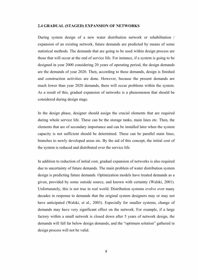
The first thing to do before running the software is the data input. Data input stage
contains identification of the following:
12
• Pipes that are going to be optimized: The user defines which pipes are going
to be included in the optimization process. In some cases, the user may not
need all of the pipes be optimized.
• Assignment of groups: Each of the pipes to be sized must be assigned to a
group. All pipes in the same group will be assigned the same diameter A
detailed discussion is given in Section 3.5.1 regarding grouping of pipes. In
brief, since it is not desirable to have pipe sizes change at every block in a
network, the user groups pipes that are to be assigned same diameter. This
reduces the number of combinations considerably.
• Assignment of candidate pipe sizes: For each of the groups, a list of candidate
pipe sizes needs to be specified. This list may include elimination of the
group as an alternative and/or cleaning of the old pipes which run parallel to
the new pipes.
• Assignment of cost functions: For every group, which cost function should be
used by the software is assigned. The cost functions represents various
conditions related to the construction and installation of pipes. The pipes
within a group can be assigned to different cost functions.
• Assignment of demands and pressure constraints at the nodes: The required
output at all nodes and the pressure, which needs to be maintained, are
specified.
After data input stage, WADISO follows the schematic flowchart of the procedure,
which is given in Figure 3.1. First, WADISO selects a pipe size combination that
meets the design criteria, i.e. pressure constraints, regardless of its cost. This is “Best
Solution”. For the next size combination, it first computes the total cost of the
combination. If the total cost of this new combination is more than that of “Best
Solution”, it is omitted and another size combination is selected. If it passes,
following tests are applied to the new combination:

13
Generation of Size Combination
Computation of Cost
Cost Test
Compare with Non-functional Combinations
Size Test
Compute Pressure Distribution
Feasible
Save Solution
Enter into File
Yes
No
Pass
Fail
Fail
Pass
Figure 3.1: Schematic Flowchart for Partial Enumeration Technique

14
Test on Size Range: The number of pipe size combinations to be tested is equal to
the product of the number of candidate sizes in each group. To reduce the number of
pipe combinations, it is required to test whether the candidate pipe sizes assigned for
groups are appropriate or some can be eliminated. To verify this, a combination
consisting of the smallest size in a group combined with the largest sizes in all other
groups is built and checked if the pressure requirement is fulfilled. If not, tested
smallest pipe size is eliminated which in turn eliminates many infeasible pipe
combinations reducing the computation time.
Cost Test: After a size combination has been found that meets all pressure
requirements, there is no need to test any other size combination that is more
expensive than this functional solution (Gessler, 1985). This cost test is most
effective in eliminating candidate solutions if it is possible to find a relatively
inexpensive functional inexpensive solution early on. Only the combinations within
Pareto optimal specifications are allowed to pass cost test. For each pipe size
combination, the program will first calculate the total cost (excluding pump cost). If
the construction cost is already more than the total cost of a previously found and
functional solution, the program will disregard this combination and proceed with the
next one.
Size Test: If a certain pipe size combination does not meet the pressure requirement,
no pipe size combination with all pipes equal or smaller than the ones of this
combination can meet the pressure requirement (Gessler, 1985). In order to perform
the size test, WADISO maintains a queue of nonfunctional combinations. This queue
is not allowed to grow too long. Otherwise, the testing of a particular size
combination against all entries in the queue requires more computation time than
evaluation of pressure distribution. During the enumeration process, the program
maintains a file of pipe size combinations that failed to meet the pressure
requirements. In brief, it will not be necessary to calculate the pressure distribution
for a combination in which all sizes are equal or less than the sizes of the
corresponding pipes in a combination stored in this file, because it could not meet
pressure requirements either.

15
If a combination passes these tests, the pressure distribution within the network is
calculated as per the given loading patterns. According to the results of this
computation, a combination is either “non-functional” or “new best solution”
Non-functional Solution: During pressure distribution computations, if it is
encountered that pressure requirement at a node cannot be satisfied, computations are
terminated, then, the combination is entered into the file of non-functional
combinations and the program proceeds with the next size combination.
New Best Solution: If the pressure requirement is met at all nodes, the algorithm has
found a solution better than an other one previously encountered. Then, it is stored as
the new best solution and the program proceeds with the next size combination. If
there are pumps, present worth of pumping cost is added to construction cost.
The procedure continues until all combinations have been enumerated. By the help of
this algorithm, the best solution will always be the global minimum in the cost
function.
Effectiveness of Tests: The effectiveness of these tests is illustrated by the following
numbers (Gessler, 1982). The percentage of combinations passing the cost test may
be around 20% for a relatively small number of combinations and may drop to
around 10% when the number of combinations reaches 100,000. The percentage of
combinations for which the pressure distribution needs to be evaluated may be as
high as 10% for small number of combinations and drops to less than 1% for large
numbers. Obviously, these numbers will vary from network to network. They are
provided here as a guideline only.
3.4. HYDRAULIC NETWORK ANALYSIS
In the optimization algorithm of WADISO, the hydraulic constraints are defined as
the minimum pressures that should be satisfied at every node. After size and cost
tests, the software calculates the pressure distribution within the network. For
network analysis, two methods are available suggested by Hardy Cross (1936): loop

16
and node methods. In WADISO, node method is applied. The terminology that will
be used hereafter is as follows:
Links : Pipes, pumps, pressure reducing valves
Nodes : Junctions between links
In a system with p links and n nodes, among which are r reservoirs, the problem has
the following unknowns:
p links (flow rates)
n-r heads
Total of p+n-r unknowns.
To find these unknowns, following equations are built:
• The energy equation between any two directly connected nodes (friction loss
equation for pipes, or characteristics curve of pumps)
• The continuity equation at all nodes, excluding the constant head nodes.
Therefore, the total number of available equations is p+n-r.
The uniqueness of the solution will not be discussed in detail herein, but simply, a
network that consists of only pipes and nodes has a single solution. In case of pumps
and valve inclusion, as long as the first derivative of the characteristic pump curve is
negative for all discharges, the uniqueness is also guaranteed.

17
3.4.1 Loop Method
1 2
34
5
6
Figure 3.2: A simple looped network In the loop method, procedure is initiated by assuming flow rates and directions for
each pipe so that the continuity is satisfied at all nodes, i.e. inflow into the nodes are
equal to the outflows, as given in Figure 3.2. Then, for every loop, friction loss is
calculated in the selected direction, clockwise in Figure 3.2. For the first trial, it is
most likely that the total headloss calculated will not be equal to zero. The key
concept in loop method is to superimpose a flowrate correction ∆Q in all pipes of a
loop either with the sense of the loop or against it. In other words, for pipes with a
positive friction loss the flow correction is added to the discharge, and in pipes with a
negative friction loss the flow correction is subtracted, or vice versa. After
application of flow rate correction to the estimated flow rates, the continuity
equations at all nodes still will be met.
Hardy Cross (1936) solved these equations for ∆Q one at a time using a Taylor
expansion of hydraulic loss equation, keeping the first two terms only. However,
convergence is very slow and gets worse with the increasing system size with this
application.

18
3.4.2 Node Method
The node method requires solving as many equations as there are nodes with
unknown heads. In the node method, the heads at the nodes are estimated, and flow
rate in each link is calculated based on these estimates. Then, the continuity at the
nodes is checked. Nevertheless, based on the head estimates, the sum will be a
residual flow rate. Cross then proceeded by assuming the heads at adjacent nodes to
be correct. One can then adjust the head at the node under consideration such that the
flow rates will balance. The resulting non-linear equations are solved by
linearization.
3.4.3 Comparison of Loop and Node Methods
• The node method has a simpler topology. This may be of particular
importance when it is necessary to temporarily eliminate a link. This may be
required if the status of a valve is changed from open to closed. In loop
method, this requires re-establishing of loops.
• In the node method, one directly solves the equations for the unknown
pressures. In the loop method, pressures are calculated at the end of whole
processes with extra calculations.
• Inclusion of pumps, pressure reducing or check valves are much easier in
node method since the devices are pressure controlled. The status of these
devices can be checked after each iteration.
3.4.4 Node Method Used in WADISO
WADISO uses the Hazen Williams friction loss equation to calculate the losses in
the pipes (Walski et al, 1990).
85,1* iii Qch = (3.1)
87.485.1 **68.10
ii
ii DC
Lc = (3.2)

19
where hi is the friction loss in pipe i in m.
Ci is the characteristic pipe coefficient for pipe i
Qi is discharge in pipe i in m3/s.
L is the length of pipe i in m.
D is the diameter of pipe i in m
Equation 3.1 can be linearized in regard to correction on the discharge to read
)85.1( 85.00
85.10 qQQcHH iiikj +=− (3.3)
where Hj and Hk are total heads at the beginning and ending node of pipe i with
Hj>Hi
Qi0 = estimated flow rate in pipe i
And Qi=Qi0+q (3.4)
where Qi is the updated flow rate in pipe i
q is the difference between updated and estimated flow rate.
Combining equations 3.3 and 3.4 to eliminate q,
85.00
0 54.046.0ii
kjii Qc
HHQQ
−+= ( 3.5)
Then the continuity equation is written, e.g. for node 2 in Figure 3.2,
054.046.054.046.02154.046.0 285.055
52585.0
22
32285.0
111 =+
−++
−++
−−− d
oo
oo
oo Q
QcHHQ
QcHHQ
QcHHQ (3.6)
where Qd2 is the amount of water withdrawn at node 2. If the estimated flow rates are
close to the correct flow rates then
20
046.046.046.0 2521 ≅+++− dooo QQQQ (3.7)
which allows us to simplify Equation 3.7 as
2585.055
385.02
285.055
85.02
85.011
185.011
12
1)12
11(1d
oooooo
QHQc
HQc
HQcQcQc
HQc
−=−−+++− (3.8)
This is the linearized continuity equation, i.e. an equation with exponents of 1 on
unknown heads H, in terms of the unknown heads at the adjacent nodes and at node
2, as well as in terms of estimated flow rates leading to node 2.
For the nodes with constant heads, e.g. for node 1, the equation is revised as:
1485.044
285.011
1 *11* roo
HAHQc
HQc
HA =−− (3.9)
where A is a very large number, for instance 105
Hr1= required head at node 1.
When all continuity equations are formulated and the proper equations at the
constant head nodes are inserted, the resulting coefficient matrix is always
symmetrical and for large networks extremely sparse. Gessler (1985) showed that the
symmetry is also preserved when pump and/or Pressure Reducing Valves are
present. The algorithm of WADISO takes advantage of both the symmetry and
sparseness when solving the continuity equations simultaneously.
3.5 STEPS OF PARTIAL ENUMARATION WITH WADISO
3.5.1 Pipe Grouping
Pipe grouping is the most useful and at the same time most critical step of the system
setup with WADISO. It is useful because by the aid of pipe grouping concept,
amount of candidate pipe combinations are reduced which in turn reduces the
computation time significantly. It is critical at the same time, because if the groups

21
are built in hands of people that have little knowledge on hydraulics, it may lead to
very unrealistic “optimum” solutions.
Generally, optimization of every pipe within a system is not required; on the
contrary, it is sometimes not desirable. For example, it is not desirable to have a main
line whose diameter changes at every junction. Similarly, a designer would not prefer
a loop with one leg’s diameter is 200mm while the parallel leg is optimized as
80mm. Consequently, designers have some common rules such as the mains and
tributaries are easily observed, having same diameters in the parallel legs of loops in
order to increase reliability of the system, etc. Thus, some pipes should have the
same diameters. With pipe grouping concept in WADISO, this can be achieved. By
this way, not only the above concepts are fulfilled, but also the computation time is
reduced.
In WADISO, grouping of pipes is accomplished by the user before the optimization
procedure starts. The user specifies which pipes should have the same diameter. For
this purpose, following concepts are useful:
• The main lines feeding whole system, i.e. taking water directly from tank,
reservoir, pump and end at another source, are grouped individually (Figure
3.3).
RESERVOIR 2
RESERVOIR 3
RESERVOIR 1
GROUP 2
GROUP 3
GROUP 1
Figure 3.3: Grouping of main lines

22
• Main tributaries feeding sub-zones form individual groups (Figure 3.4).
GROUP 6
GROUP 5
GROUP 4
RESERVOIR 1
Figure 3.4: Grouping of main tributaries
• Parallel legs of a loop form one group (Figure 3.5).
GROUP 8
GROUP 7
Figure 3.5: Grouping of parallel pipes

23
The groups may include any number of pipes, even if a single pipe can form a group
if it is desired to be optimized. However, number of groups within WADISO is
limited to 15, i.e. maximum number of groups that can be formed is equal to 15. This
is again to reduce computation time. Due to this limitation, pipe groups should be
selected very carefully, only those pipes that have significant effect on the global
cost of the system should be included in groups. In other words, the smaller branches
need not be included in the procedure. The change of a pipe’s diameter from 125mm
to 100mm will not be very significant on the global cost. However, the reduction of a
3000m-long main line’s diameter from 1000mm to 800mm will produce great cost
savings.
Pipe grouping concept reduces computation time and provides a clear conveyance
layout to the system. However, pipe grouping should be handled carefully with
hydraulic principles kept in mind. As stated before, all the pipes in a group will have
the same diameter at the end of optimization. As an example, Figure 3.6 is given.
Region 1 is an industrial zone where demands are higher requiring larger diameters.
On the other hand, Region 3 is a commercial zone with moderate demands and
Region 2 is composed of residential dwellings, which requires relatively low
demands as compared to Region 1, which results in smaller diameters. If all the pipes
in the three main lines are assigned to the same group, they will have the same
diameter at the end of optimization. Since the demands are higher at Region 1, larger
diameter main line will be assigned by WADISO due to pressure requirements.
Although the demands are smaller for Region 2 and 3, because they are in the same
group with Main Line 1, they will be assigned the same diameter of main line 1. In
this case, the diameter of Main Line 1 will be governing one; main lines 2 and 3 will
be unnecessarily assigned larger diameters. However, if all main lines are assigned to
individual groups, they will have different diameters as per demands of the
corresponding regions, Main Line 1 having the largest diameter where Main Line 2
has the smallest.

24
MAIN LINE 3
MAIN LINE 2
MAIN LINE 1REGION 1 (INDUSTRIAL)
REGION 2 (RESIDENTIAL)
REGION 3(COMMERCIAL)
Figure 3.6: Sample Network For Pipe Grouping 3.5.2 Pipe Size Assignment
In the pipe size assignment step, the candidate pipe sizes for each group are listed.
Although it is possible, the list for a group does not need to include all commercially
available pipe sizes, since having too many candidate pipe sizes for groups will
increase computation time. Thus, the candidate pipe sizes should be “reasonable”. To
find the reasonable candidate pipe sizes, following procedure can be followed:
• Using rules-of-thumb and experience and trial-and-error method, assign
preliminary pipe sizes for every pipe in the system. This is also a pre-
requisite for WADISO. Before running optimization module, program tries to
balance the system, thus in the very beginning, preliminary diameters of all
pipes should be assigned.

25
• Assign one lower and one upper commercially available pipe diameter
together with the preliminary diameter for every group and run the first
optimization trial (Table 3.1). This will last for 4~12 hours depending on the
system size and number of groups.
Table 3.1: Candidate pipe sizes for first run
• Check the results of the optimization. Identify the groups in which program
assigns the lowest available candidate size. This may mean that if there were
lower diameters, the program may assign it (lower) to the group. To ensure
the results and to give relaxation for the program, assign two more lower
diameters. Similarly, if the program assigns the upper diameter for a group,
assign two more upper diameters. (Table 3.2.)
PRELIMINARY
DIAMETERS 200,00 110,00 500,00 250,00 200,00
GROUP1 GROUP2GROUP3 GROUP4 GROUP5
CANDIDATE DIAMETERS (mm) 180,00 90,00 450,00 225,00 180,00
200,00 110,00 500,00 250,00 200,00 225,00 125,00 560,00 280,00 225,00
OPTIMUM DIAMETERS (mm) 180,00 110,00 450,00 225,00 180,00

26
Table 3.2: Revised Candidate Pipe Sizes for Second Run
• Perform the optimization and repeat the previous step until the program
assigns diameters to group that are neither the available upper nor the lower
ones (Table 3.3).
Table 3.3: Final Candidate Diameters and Optimum Sizes
PREVIOUS OPTIMUM DIAMETERS (mm) 160,00 110,00 400,00 250,00 160,00
GROUP1 GROUP2 GROUP3 GROUP4 GROUP5
CANDIDATE DIAMETERS (mm) 140,00 90,00 355,00 180,00 140,00
160,00 110,00 400,00 200,00 160,00
180,00 125,00 450,00 225,00 180,00
250,00
280,00
OPTIMUM DIAMETERS (mm) 160,00 110,00 400,00 250,00 160,00
As can be seen from Table 3.1, for the first run, due to available candidate pipe sizes,
WADISO assigned 180mm for Group 1 and 225mm for Group 4, which are the main
lines of the system. Then in the second run program assigns 160mm for Group 1 and
250mm for Group 4 since there are more available diameters. Finally, to check if
more changes would have occurred when 280mm were in the candidate sizes, it is
included in the candidate sizes list. At the same time, to reduce computation time,
PREVIOUS OPTIMUM DIAMETERS (mm)
180,00 110,00 450,00 225,00 180,00
GROUP1 GROUP2 GROUP3 GROUP4 GROUP5
CANDIDATE DIAMETERS (mm) 140,00 90,00 355,00 180,00 140,00
160,00 110,00 400,00 200,00 160,00
180,00 125,00 450,00 225,00 180,00
200,00 500,00 250,00 200,00
OPTIMUM DIAMETERS (mm) 160,00 110,00 400,00 250,00 160,00

27
candidate sizes from Groups 3 and 5 are reduced to three, and according the results,
WADISO assigned all the diameters for the groups that were neither the lowest nor
the highest available ones.
As discussed previously, cleaning / rehabilitation is also an alternative for new pipe
installation. One can assign this option during optimization with WADISO. In this
case, the preliminary diameters should be the real world diameter of the group. Then,
assumed Hazen Williams coefficient of pipes after cleaning is given to program
together with its associated price function. In this option, WADISO determines if it
will be more economical when the constructed system is cleaned and rehabilitated or
the existing pipes should be replaced by new ones.
One of the drawbacks of optimization methods is to reduce the reliability of the
system to save costs. If the designer decides that, some groups formed in the
previous steps can be eliminated, then this option can also be introduced into
WADISO. Then, the program will test all the combinations including elimination of
the said groups. As the result, it may produce results including elimination provided
that the specified pressure restraints at nodes are all satisfied. However, it should be
kept in mind that these pressure constraints are satisfied with the given steady state
loading pattern(s). The reliability of the system should be checked with Extended
Period Simulation Analysis and with other critical Steady State Loading Patterns.
3.5.3 Price Functions
Within the optimization process with enumeration, number of combinations of pipes
are built, and then compared with each other to find the most economical
combination that meets the restrictions. Within this process, pipes are valued by
multiplication of their lengths times the assigned price function, - price function of a
pipe is the cost per meter of the pipe - and finally all the costs of pipes are added
resulting in the cost of the whole system. Thus, the only cost related part of
optimization with WADISO is the price function. This obviously requires that the
price functions should not only be considered as the pipe material costs, but should
also include construction costs (excavation, fill, bedding transportation etc.), special

28
crossing costs (crossing under a heavily loaded motorway, river etc.), pipe fittings’
costs (elbows, collars, branching fittings, dead-end fittings etc.) and all the other
costs specific to the projects.
In the past, various attempts have been made to find the price functions of the pipes
to assist planners and developers such as Clark, et al. (2002), or the outcome of the
survey performed by American Environmental Protection Agency (2001). Although
all these gives rough estimates that can be used for master planning stage, detailed
cost analysis should be performed for each project considering the latest market
conditions (e.g. rise of steel prices, advances in pipe material chemistry, new
construction technologies etc.).
In the recent years, there have been advances in pipe chemistry that enables
designers to use different kinds of pipes within their designs, such as GRP (glass
fiber reinforced polyester), HDPE (high density polyethylene), ductile iron etc. All of
these pipe materials have advantages depending on the point of view. One material
may have very well hydraulic properties (such as low friction loss), but another one
may have dramatically low prices. Thus, there is not a universal law that rules the use
of material in water distribution networks.
In addition to cost perspective, other factors limit the use of a material in every
aspect of design. For example, GRP pipes can be very well applied in water
transmission lines. However, due to their brittle characteristics, they are not advised
for distribution lines. In short, there are factors that cannot be represented in
mathematical cost functions but which dictates the use of a material.
All pipe materials have different material characteristics and they do also have
different construction methodologies, fittings installation etc. A brief summary for
three basic types of pipe materials is as follows:
29
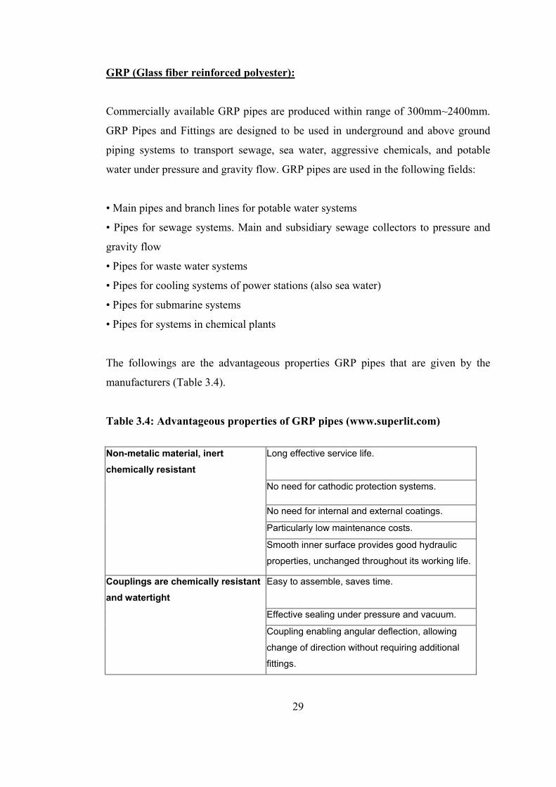
GRP (Glass fiber reinforced polyester):
Commercially available GRP pipes are produced within range of 300mm~2400mm.
GRP Pipes and Fittings are designed to be used in underground and above ground
piping systems to transport sewage, sea water, aggressive chemicals, and potable
water under pressure and gravity flow. GRP pipes are used in the following fields:
• Main pipes and branch lines for potable water systems
• Pipes for sewage systems. Main and subsidiary sewage collectors to pressure and
gravity flow
• Pipes for waste water systems
• Pipes for cooling systems of power stations (also sea water)
• Pipes for submarine systems
• Pipes for systems in chemical plants
The followings are the advantageous properties GRP pipes that are given by the
manufacturers (Table 3.4).
Table 3.4: Advantageous properties of GRP pipes (www.superlit.com)
Non-metalic material, inert chemically resistant
Long effective service life.
No need for cathodic protection systems.
No need for internal and external coatings.
Particularly low maintenance costs.
Smooth inner surface provides good hydraulic
properties, unchanged throughout its working life.
Couplings are chemically resistant and watertight
Easy to assemble, saves time.
Effective sealing under pressure and vacuum.
Coupling enabling angular deflection, allowing
change of direction without requiring additional
fittings.

30
Table 3.4 Continued
Low weight (about 1/10 of a concrete pipe, 1/4 of steel pipe)
Quick and easy installation. There is no need for
heavy equipment to transport pipes.
Cheap transportation.
Long pipe sections Few connections, very fast installation.
Excellent inner smoothness High Hazen-Williams factor, significant energy
savings.
The energy savings in time may be equivalent to
the purchase cost of the pipe.
Figure 3.7 Connection of GRP Pipes (www.superlit.com)

31
Figure 3.8 GRP Water Transmission Line (www.superlit.com)
HDPE (High density polyethylene pipes): HDPE pipe diameters vary between
75mm up to 1600mm depending on the pressure class. HDPE pipes are applied in the
following fields:
• Surface and Underground Drinking Water Networks
• Natural Gas Systems and Networks
• Irrigation Systems
• Drainage and Sewerage Systems
• Sea Discharging Systems
• Waste Water Systems
• Solid Waste Drainage Systems
• Fire Water and Cooling Water Systems
• Geothermal Systems
• Pharmaceutical and Chemical Industry / Sanitary Appliances
• Aggressive Fluid Systems

32
Basic properties of HDPE pipes, which make them advantageous among others,
given by manufacturers are as follows (www.superlit.com):
• 50 years of service life guarantee
• Perfect corrosion resistance
• High resistance to chemical agents
• Good flexibility
• Light weight, easy transport, loading, unloading and installation
• Various jointing methods
• Capability of assembling in and/or out of channel during installation
• High elasticity (18-20 times of its diameter) , minimum fittings usage
• Perfect adaptation to the field conditions, suitable for seismic area
• Perfect welding and leak-proof characteristic
• Resistance to UV rays and low temperature conductivity
• High resistance to cracking and impact
• Production of all pressure classes between 2,5 bars and 32 bars ,
• and also optional production according to the clients’ requirements
• Resistant to the sudden pressure increases known as “ Water Hammer “
• Low operating cost
• Easy repairs by strangle technique
• Mobile production facility for huge projects
HDPE pipes are classified according to pressure class as SDR value. SDR value
stands for the "Standard Diameter Ratio" which is the outside diameter divided by
the wall thickness. A 2" SDR 7 product would have the outside diameter of 2.375"
and a wall thickness of 0.339" (2.375/0.339 = 7).
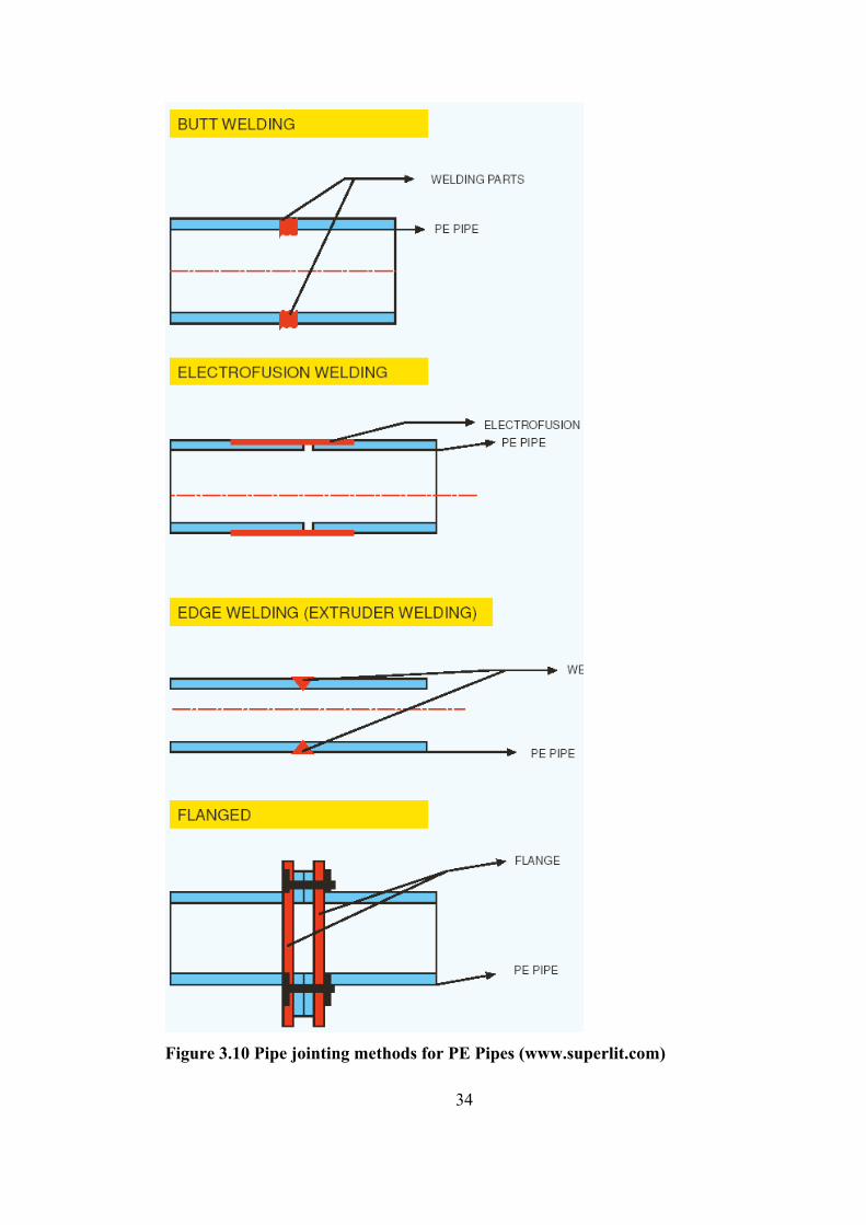
Pipe jointing methods used for HDPE pipes are butt-welding method, electrofusion
welding, electrofusion coupling, edge welding and flanged (Figure 3.10).
Butt-welding can be performed for PE Pipes with wall thickness greater than 4mm.
The two pipes that are going to be welded should have the same wall thickness.

33
Welding can be performed inside or outside the trench. However, considering the
width of welding machine, trench should be excavated larger than required to
perform welding inside. General application is giving a reasonable radius
(approximately 18 x pipe diameter) to the PE pipe inside of the trench to take the
edge out of the trench, and then perform welding outside of the trench. No extra
fittings are required for butt-welding.
Electrofusion welding can be used for pipes up to Ø110mm for pipes having
different wall thickness.
When butt-welding cannot be carried out, the electrofusion-coupler is the ideal for
big diameters and long pipe lengths. The electrofusion coupler is a joint with an
incorporated heating element that (connected to the automatic welding machine)
absorbs the necessary heat for welding (Figure 3.9). Inside the coupler, there are
notches for the insertion of the pieces to be welded, which will join up in the middle
to make the surface more sliding. (These notches can be removed by a knife) The
welding pressure is given by the coupler which shrinks because of the temperature.
During welding, in order to avoid the softening of material that causes contractions
on the pipe, the external and central areas of the coupler do not melt. The contraction
is uniformly distributed during welding.
Figure 3.9 Electrofusion coupling of PE Pipes (www.superlit.com)
Edge welding and flanged jointing are applied for gravity pipelines.
34
Figure 3.10 Pipe jointing methods for PE Pipes (www.superlit.com)

35
Ductile Iron Pipes: Since its first introduction into the market in 1955, ductile iron
has been extensively used in wide range of sectors including water and waste water
systems (Figure 3.11).
Figure 3.11 Ductile Iron production in the past for all sectors (www.ductile.org)
Ductile Iron not only retains all of Cast Iron's attractive qualities, such as
machinability and corrosion resistance, but also provides additional strength,
toughness, and ductility. It is lighter, stronger, more durable and more cost effective
than Cast Iron. Although its chemical properties are similar to those of Cast Iron,
Ductile Iron incorporates significant casting refinements, additional metallurgical
processes, and superior quality control. Ductile Iron's improved qualities are derived
from an improved manufacturing process that changes the character of the graphite
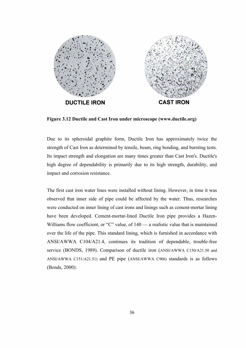
content of the iron. Ductile Iron's graphite form is spheroidal, or nodular, instead of
the flake form found in Cast Iron (Figure 3.12). This change in graphite form is
accomplished by adding an inoculant, usually magnesium, to molten iron of
appropriate composition during manufacture.
Year
36
Figure 3.12 Ductile and Cast Iron under microscope (www.ductile.org)
Due to its spheroidal graphite form, Ductile Iron has approximately twice the
strength of Cast Iron as determined by tensile, beam, ring bending, and bursting tests.
Its impact strength and elongation are many times greater than Cast Iron's. Ductile's
high degree of dependability is primarily due to its high strength, durability, and
impact and corrosion resistance.
The first cast iron water lines were installed without lining. However, in time it was
observed that inner side of pipe could be affected by the water. Thus, researches
were conducted on inner lining of cast irons and linings such as cement-mortar lining
have been developed. Cement-mortar-lined Ductile Iron pipe provides a Hazen-
Williams flow coefficient, or “C” value, of 140 — a realistic value that is maintained
over the life of the pipe. This standard lining, which is furnished in accordance with
ANSI/AWWA C104/A21.4, continues its tradition of dependable, trouble-free
service (BONDS, 1989). Comparison of ductile iron (ANSI/AWWA C150/A21.50 and
ANSI/AWWA C151/A21.51) and PE pipe (ANSI/AWWA C906) standards is as follows
(Bonds, 2000):

37
Table 3.5: Comparison of ductile iron (ANSI/AWWA C150/A21.50 and ANSI/AWWA C151/A21.51) and PE pipe (ANSI/AWWA C906) standards
Ductile Iron Pipe HDPE Pipe ANSI/AWWA C150/A21.50 ANSI/AWWA C906
TOPIC
ANSI/AWWA C151/A21.51 Sizes 3”-64” 4”-63” Laying Lengths
18’, 20’ 40’
Rated up to 350 psi. Pressure Class 150, 200, 250, 300, & 350.
Pressure Class / Ratings
Higher pressures may be designed.
Dependent on material code: 40 to 198 psi for PE 2406 or PE 3406; 51 to 254 psi for PE 3408.Rated up to 254 psi for 20-inch diameter and smaller. Due to manufacturers limited extrusion capabilities for wall thicknesses >3-inches, ratings may be progressively reduced with increasing sizes greater than 20-inches in diameter. Flexible material; internal pressure design only.
Method of Design
Designed as a flexible conduit. Separate design for internal pressure (hoop stress equation) and external load (bending stress and deflection). Casting tolerance and service allowance added to net thickness.
External load design is not covered by a standard.
Internal Pressure Design
Pressure Class: stress due to working pressure plus surge pressure cannot exceed the minimum yield strength of 42,000 psi ÷ 2.0 safety factor.
Pressure Rating: Stress due to working pressure cannot exceed the Hydrostatic Design Basis (1,600 psi) ÷ 2.0 safety factor (Hydrostatic Design Stress = 800 psi) for PE 3408. Any surge pressure compromises the safety factor.
Surge Allowance
Nominal surge allowance is 100 psi (based on an instantaneous velocity change of approximately 2 fps), however, actual anticipated surge pressures should be used.
Not Included. Surge pressures are allowed to compromise the “design factor” which results in a reduction in the safety factor below 2.0.
External Load Design
Prism load + truck load. Ring bending stress limited to 48,000 psi, which is 1/2 the minimum ultimate bending strength. Deflection is limited to 3% of the outside diameter of the pipe, which is 1/2 of the deflection that might damage the cement-mortar lining. The larger of these two thicknesses governs and is taken as the net thickness.
None discussed in standard.
Live Load AASHTO H20, assuming a single 16,000 lb. concentrated wheel load. Impact factor is 1.5 for all depths.
None discussed in standard.

38
Table 3.5 Continued
Pressure Design: 2.0 (including surge) based on minimum tensile yield strength of 42,000 psi.
A “Design Factor” is used in the internal pressure design formula. This factor is simply the inverse of the more common “Safety Factor.” This “Design Factor,” in reality, is not a constant number. The design formula for hdpe pipe ignores surge pressures by merely increasing the “Design Factor,” thereby, reducing the “Safety Factor,” to compensate for them.
Factor of Safety
External Load Design: 2.0 for bending based on minimum ultimate ring bending strength of 96,000 psi, or 1.5 for bending based on minimum ring yield bending strength of 72,000 psi. 2.0 for deflection for cement-mortar-lined pipe. Note: Actual safety factors are greater than the nominal safety factors due to the addition of the service allowance and casting tolerance in the design procedure.
Ignoring surge pressures, the “Design Factor” is 0.5 (“Safety Factor” is 2.0). Acknowledging surge pressures, the “Design Factor” is >0.5 (“Safety Factor” is < 2.0).
Five specified laying conditions (Types 1-5).
Specified Trench Conditions Conservative E’ and soil strength
parameters listed. Type 1 (flat bottom trench, loose backfill) or Type 2 (flat bottom trench, backfill lightly consolidated to centerline of pipe) are adequate for most applications.
None.
Hydrostatic Testing
Each pipe tested to a minimum of 500 psi for at least 10 seconds at full pressure.
Only one pipe size from three size ranges (4- to 12-, 14- to 20-, and ≥ 24-inch) are subjected to an elevated temperature sustained pressure test semiannually. Also, only one pipe per production run may be subject to a quick burst test. A ring tensile test or a five-second pressure test can be substituted for this test.
Factory Tests
At least one sample during each casting period of approximately 3 hours shall be tested for tensile strength; must show minimum yield of 42,000 psi, minimum ultimate of 60,000 psi and a minimum elongation of 10%. At least one Charpy impact sample shall be taken per hour (minimum 7 ft-lb.), with an additional low-temperature impact test (minimum 3 ft-lb.) made from at least 10% of the sample coupons taken for the normal Charpy impact test.
Bend-back or elongation-at-break; once per production run. Ring tensile, quick burst, or fivesecond pressure test; once per production run.Melt flow index; once per day. Density; once per day. Carbon black content; once per production run.

39
Pipe Fittings: In the most simplest form, pipe fittings are the materials that are used
to join pipes or used to provide junctions for branching pipes. There are numerous
kinds of pipe fittings, the common ones being (www.superlit.com):
• Flanges (Figure 3.13)
Figure 3.13: Flanges
• Bends (45°, 90°), to provide deflection from alignment (Figures 3.14, 3.15)
Figure 3.14: Bends (90°)

40
Figure 3.15: Bends (45°)
• Tees, to provide 90° junction (Figures 3.16, 3.17)
Figure 3.16: Equal Tee

41
Figure 3.17: Unequal tee
• Reducers, to connect a larger diameter with a smaller one in series
(Figure3.18)
Figure 3.18: Reducer
Depending on the need, there are also other fittings such as:
• Flange Tees
• Blind Flanges
• Saddle service tees
• Hydrant Connections

42
• Adapters
The prices of fittings depends on the following:
• Material types of connecting pipes
• Required pressure strength
• Diameters of connecting pipes
• Methodology to connect pipes and fittings (e.g. for HDPE pipes connection
with electrofusion or welding)
As an example, a simple junction is given in Figure 3.19.
D1 D1
D2
25m 25m
25m
Figure 3.19: Example Fitting Layout (with unequal tee)
According to Unit Prices announced by Bank of Provinces (İller Bankası) and State
Hydraulic Works (DSİ) for year 2004, the total cost of the system with various
diameters are given in Table 3.6 and Figure 3.20

43
Table 3.6: The total cost of the system (fitting with unequal tee)
D1 D2 COST OF PIPES COST WITH TEE 110 90 414.35 YTL 484.57 YTL 125 90 494.20 YTL 579.33 YTL 140 90 588.08 YTL 708.45 YTL 160 90 713.23 YTL 863.48 YTL 180 90 864.33 YTL 1,055.44 YTL 200 90 1,015.43 YTL 1,272.45 YTL 225 90 1,248.43 YTL 1,578.78 YTL 250 90 1,481.45 YTL 1,922.06 YTL 280 90 1,837.70 YTL 2,429.93 YTL 315 90 2,253.38 YTL 2,910.81 YTL
0.00 YTL500.00 YTL
1,000.00 YTL1,500.00 YTL2,000.00 YTL2,500.00 YTL3,000.00 YTL3,500.00 YTL
110/9
0
125/9
0
140/9
0
160/9
0
180/9
0
200/9
0
225/9
0
250/9
0
280/9
0
315/9
0
Cost of Pipes Cost incl. Tee
Figure 3.20: The total cost of the system (fitting with unequal tee)
As it is observed from Figure 3.20, the total cost may increase up to 30% with
inclusion of the cost of tee.
In order to include the effect of fittings in the optimization procedure with any
software below steps has to followed:
• Every fitting has to be selected as per the pressure class individually; there
should be no over-design such as installing a SDR 7,4 and PN25 atm fitting

44
for PE pipes where SDR 17 and PN10 atm is sufficient. Similarly, no under-
design should be allowed to prevent damages.
• While selecting pipe sizes for the system, price of fittings should also be
considered.
In WADISO, the price functions are input to the software as the price per length.
However, as given above, the price of fittings are dependent on pressure classes and
the diameters of pipes connected to them. This creates a vicious circle: in order to
include the price of fitting, diameters have to be known, but the optimization, i.e.
inclusion of fitting prices in price function, is performed to determine the diameters.
As the result, since there is no mathematical relationship between the fittings and the
pipes, it is almost impossible to consider effect of fittings during optimization with
WADISO.
As the conclusion, in order to have a reasonable optimum solution with WADISO,
designer should have a good knowledge on available pipe materials, their conformity
to his project area, recent market prices, construction and installation technologies
and their corresponding prices. For a general design of a water distribution system
with WADISO, the following items can be included in price functions for the design
of a system:
Table 3.7: Activities / materials for HDPE Price Function
EXCAVATION WORKS
Trench excavation (without explosives)
Fill
Bedding & Compaction
PIPE RELATED
Pressure Test Before Laying
Connection of HDPE Pipes with Butt Welding
Laying of HDPE Pipes
HDPE Pipe material

45
Table 3.8 Activities / materials for Steel or Ductile Price Function
EXCAVATION WORKS
Trench excavation (with/without explosives)
Fill
Bedding & Compaction
PIPE WORKS
Pressure Test Before Laying
Welding
Inner insulation of welded ends
Outer insulation of welded ends
Laying
Price of pipe material
Cathodic protection (~2% of pipe price)
However, it should be kept in mind that the effects that cannot be included in price
functions should be checked by the designer manually.
3.5.3.1 Price Functions for the Case Study
To use in the Case Study presented in Chapter 4, three types of materials are selected
as suitable for the network and their corresponding price functions are built.
• HDPE (High density polyethylene)
• Steel Pipe
• Ductile Iron Pipe
To calculate the price function of each material in YTL/m, unit prices announced by
Devlet Su İşleri (DSİ-State Hydraulic Works) and İller Bankası (Bank of Provinces)
are used. Additionally, a market search has been performed including major pipe
manufacturers and approximate market prices of pipe materials are gathered. Further
to above, unit prices given by United States Environmental Agency as the result of a
broad survey performed within USA are also used.

46
HDPE Pipes Price Function: Standard diameters available for HDPE Pipes vary
between 16mm up to 1600mm depending on the pressure class. Because the
pressures are less than 100m, pipes with PN10 - SDR11 are selected for the study.
Price analyses are performed for pipe diameters 90, 110,125, 140, 160, 180, 200,
225, 250, 280, 315, 355, 400, 450, 500, 560 and 630mm.
According to information gathered from hydraulic designers, typical trench cross-
section for HDPE Pipes is given in Figure 3.21. From Figure 3.21, calculated
excavation, bedding and fill volumes are given in Table 3.9, for the mentioned
diameters.
To calculate the corresponding construction related works, unit prices of State
Hydraulic Works are used for the following items:
• Trench excavation (without explosives)
• Fill
• Bedding & Compaction
Regarding pipe related works, the following items are taken from both State
Hydraulic Works and Bank of Provinces Unit Price Books:
• Pressure Test before Laying
• Connection of HDPE Pipes with Butt Welding
• Laying of HDPE Pipes
• HDPE Pipe resistant to 10 atm
As discussed in Section 3.5.3, there are various methods for joining pipes. In this
study, because all the pipes are of the same material and assuming that all pipes have
the same wall thickness, jointing method is assumed as butt welding. Unfortunately,
due to reasons g iven in the same section, price of fittings and jointing costs at
fittings cannot be included in the optimization.

B
COM
PACT
ED F
ILL
/ G
ÖM
LEK
TABA
KASI
BED
DIN
G /
YA
STIK
TAB
AKAS
I
UPP
ER F
ILL
NO
CO
MPA
CTIO
N
(EXC
EPT
RO
AD C
RO
SSIN
G)
ÜST
TAB
AKA
SIKIŞT
IRIL
MAM
IŞ D
OLG
U(Y
OL
GEÇ
İŞLE
Rİ
HAR
İÇ)
Figu
re 3
.21:
Typ
ical
tren
ch c
ross
-sec
tion
for
HD
PE P
ipes
47
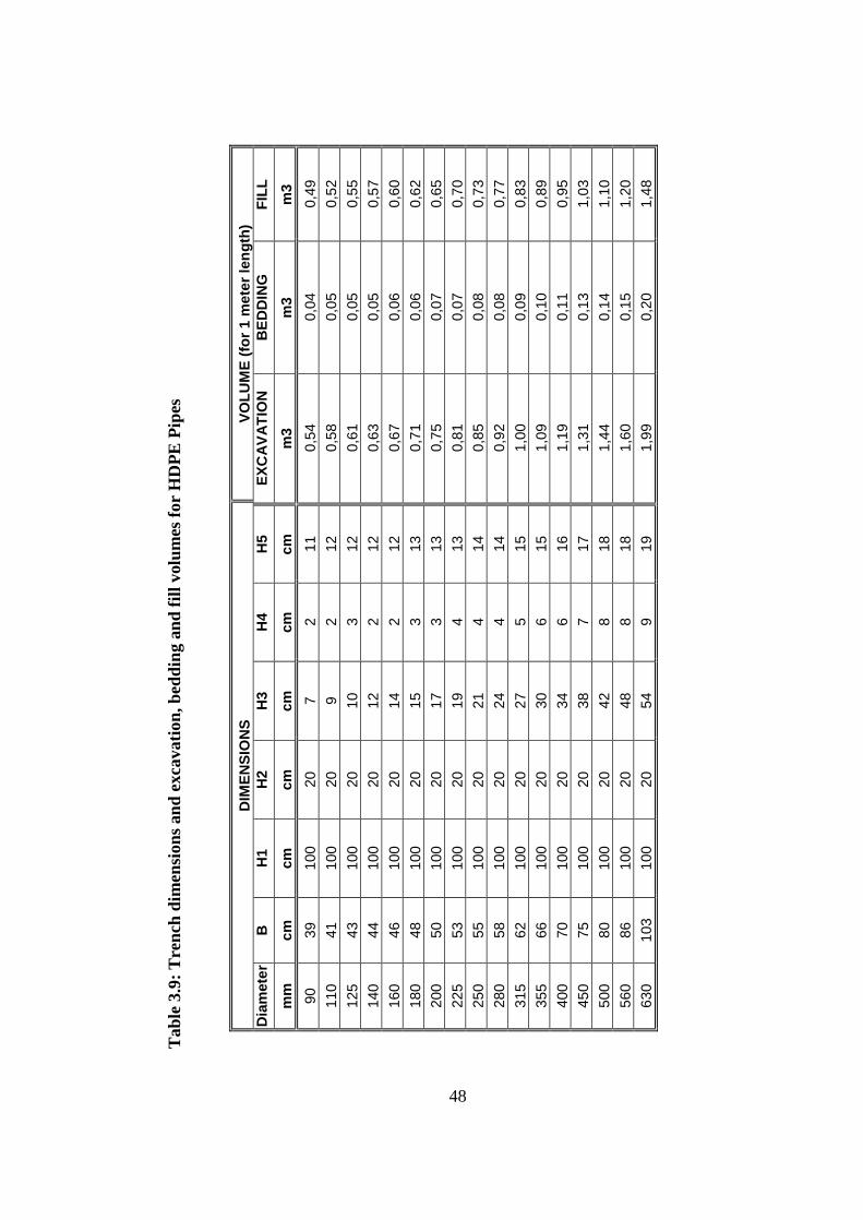
Tab
le 3
.9: T
renc
h di
men
sion
s and
exc
avat
ion,
bed
ding
and
fill
volu
mes
for
HD
PE P
ipes
DIM
ENSI
ON
S VO
LUM
E (fo
r 1 m
eter
leng
th)
Dia
met
er
B
H1
H2
H3
H4
H5
EXC
AVA
TIO
N
BED
DIN
G
FILL
m
m
cm
cm
cm
cm
cm
cm
m3
m3
m3
90
39
100
20
7 2
11
0,54
0,
04
0,49
11
0 41
10
0 20
9
2 12
0,
58
0,05
0,
52
125
43
100
20
10
3 12
0,
61
0,05
0,
55
140
44
100
20
12
2 12
0,
63
0,05
0,
57
160
46
100
20
14
2 12
0,
67
0,06
0,
60
180
48
100
20
15
3 13
0,
71
0,06
0,
62
200
50
100
20
17
3 13
0,
75
0,07
0,
65
225
53
100
20
19
4 13
0,
81
0,07
0,
70
250
55
100
20
21
4 14
0,
85
0,08
0,
73
280
58
100
20
24
4 14
0,
92
0,08
0,
77
315
62
100
20
27
5 15
1,
00
0,09
0,
83
355
66
100
20
30
6 15
1,
09
0,10
0,
89
400
70
100
20
34
6 16
1,
19
0,11
0,
95
450
75
100
20
38
7 17
1,
31
0,13
1,
03
500
80
100
20
42
8 18
1,
44
0,14
1,
10
560
86
100
20
48
8 18
1,
60
0,15
1,
20
630
103
100
20
54
9 19
1,
99
0,20
1,
48
48
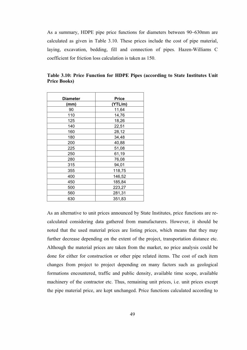
49
As a summary, HDPE pipe price functions for diameters between 90~630mm are
calculated as given in Table 3.10. These prices include the cost of pipe material,
laying, excavation, bedding, fill and connection of pipes. Hazen-Williams C
coefficient for friction loss calculation is taken as 150.
Table 3.10: Price Function for HDPE Pipes (according to State Institutes Unit Price Books)
Diameter Price (mm) (YTL/m)
90 11,64 110 14,76 125 18,26 140 22,51 160 28,12 180 34,48 200 40,88 225 51,08 250 61,19 280 76,08 315 94,01 355 118,75 400 146,52 450 185,84 500 223,27 560 281,31 630 351,83
As an alternative to unit prices announced by State Institutes, price functions are re-
calculated considering data gathered from manufacturers. However, it should be
noted that the used material prices are listing prices, which means that they may
further decrease depending on the extent of the project, transportation distance etc.
Although the material prices are taken from the market, no price analysis could be
done for either for construction or other pipe related items. The cost of each item
changes from project to project depending on many factors such as geological
formations encountered, traffic and public density, available time scope, available
machinery of the contractor etc. Thus, remaining unit prices, i.e. unit prices except
the pipe material price, are kept unchanged. Price functions calculated according to

50
market data are given in Table 3.11. It is observed that these unit prices are lower
than the ones obtained from state unit price books.
Table 3.11: Price Function for HDPE Pipes according to market data
Dia Price mm YTL/m 90 9,87 110 12,75 125 15,27 140 18,08 160 22,47 180 26,98 200 32,08 225 39,63 250 47,53 280 61,40 315 76,54 355 95,27 400 118,41 450 148,12 500 179,26 560 222,33 630 282,06
Steel Pipes Price Function: An alternative to HDPE pipes given in the
aforementioned unit price books is steel pipes. However, there were two difficulties:
available unit prices for steel pipes in State Hydraulic Works unit price book starts
from pipes with diameter equal to 500mm. and secondly the minimum pressure class
is 16atm. To find the unit prices for the diameters used in the previous optimizations,
a polyline is fitted to available data and extrapolation is done for lower diameters.
The pressure class is kept as 16atm since there is no data available regarding the
relationship of 10atm pressure class and 16atm pressure class prices of same
diameters. Material unit prices obtained by this method are given in Table 3.12 and
Figure 3.22.

51
Table 3.12: Material unit prices for steel
Dia Price mm YTL/m 80 8,52 100 11,05 125 14,4375 150 18,075 200 26,1 225 30,4875 250 35,125 300 45,15 350 56,175 400 68,2 450 81,225 500 95,25 600 126,3 650 143,325 700 161,35 750 180,375 800 200,4 850 221,425 900 243,45
1000 290,5

52
0
50
100
150
200
250
300
350
0 200 400 600 800 1000 1200Diameter (mm)
YTL/
m
Available Data Fitted and Extrapolated Data
Figure 3.22: Material unit prices for steel

53
Similar to HDPE, pipes, typical trench cross-section for steel pipes is gathered from
professions and given in Figure 3.23. From Figure 3.23 calculated excavation,
bedding and fill volumes are given in Table 3.14 for diameters between 100~600mm.
Construction related works for steel pipes are taken same as those for HDPE pipe,
but pipe related items are changed / added as follows:
• Pressure Test Before Laying
• Welding
• Inner insulation of welded ends
• Outer insulation of welded ends
• Laying
• Steel Pipe resistant to 16 Atm
• Cathodic protection (~2% of pipe price)
Unit price of inner and outer insulation items are calculated by extrapolation similar
to material pipe prices. Cathodic protection item is taken as app. ~2% of pipe price
after discussions with experienced engineers. No fitting or collar cost is included in
the price functions. Hazen-Williams C coefficient for friction loss calculation is
taken as 130. Resulting unit prices are given in Table 3.13.
Table 3.13: Unit prices for steel pipes Diameter Price
mm YTL/m 100 15,84 125 20,10 150 24,82 200 34,56 250 45,29 300 57,34 350 70,59 400 82,57 450 98,27 500 114,54 600 151,39

B
TYPE
1 O
R CL
ASS
B PI
PE B
EDD
ING
AN
D P
ROTE
CTIO
N /
Ti
p 1
Yastık
ve
Koru
ma
Taba
kası
UPP
ER F
ILL
NO
CO
MPA
CTIO
N
(EXC
EPT
ROAD
CRO
SSIN
G)
ÜST
TAB
AKA
SIKIŞT
IRIL
MAM
IŞ D
OLG
U(Y
OL
GEÇ
İŞLE
Rİ
HAR
İÇ)
Figu
re 3
.23:
Typ
ical
tren
ch c
ross
-sec
tion
for
stee
l pip
es (u
nits
in c
m)
54
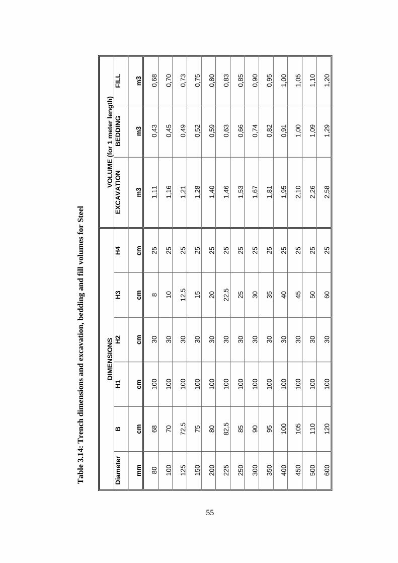
Tab
le 3
.14:
Tre
nch
dim
ensi
ons a
nd e
xcav
atio
n, b
eddi
ng a
nd fi
ll vo
lum
es fo
r St
eel
DIM
ENSI
ON
S VO
LUM
E (fo
r 1 m
eter
leng
th)
Dia
met
er
B
H1
H2
H3
H4
EXC
AVA
TIO
N
BED
DIN
G
FILL
mm
cm
cm
cm
cm
cm
m
3 m
3 m
3
80
68
100
30
8 25
1,
11
0,43
0,
68
100
70
100
30
10
25
1,16
0,
45
0,70
125
72,5
10
0 30
12
,5
25
1,21
0,
49
0,73
150
75
100
30
15
25
1,28
0,
52
0,75
200
80
100
30
20
25
1,40
0,
59
0,80
225
82,5
10
0 30
22
,5
25
1,46
0,
63
0,83
250
85
100
30
25
25
1,53
0,
66
0,85
300
90
100
30
30
25
1,67
0,
74
0,90
350
95
100
30
35
25
1,81
0,
82
0,95
400
100
100
30
40
25
1,95
0,
91
1,00
450
105
100
30
45
25
2,10
1,
00
1,05
500
110
100
30
50
25
2,26
1,
09
1,10
600
120
100
30
60
25
2,58
1,
29
1,20
55

56
Price Functions for Ductile Iron Pipes: Ductile iron pipes has always been a
primary choice of designers for water distribution networks. To perform the
optimization with ductile iron pipes, price function analysis are performed using
same items with the steel pipes. Unfortunately, no material unit price for ductile iron
pipes is announced by either State Hydraulic Works or Bank of Provinces. Thus, a
market search is conducted and material unit prices are gathered. For the pipes, using
the same price items given for steel pipes, price functions for ductile iron pipes are
obtained as given in Table 3.15. The unit prices include internal lining of cement
(ISO4179) by centrifugal process and external coating by metallic Zinc (ISO8179),
and then coverage by bituminous (asphalt) paint (BS 3416). Similar to steel pipes,
Hazen-Williams C coefficient for friction loss calculation is taken as 130 also for
ductile iron pipes. No fitting or collar cost is included in the price functions.
Table 3.15: Price Function for Ductile Iron Pipes
Dia Price mm YTL/m 100 16,19 125 17,51 150 19,04 200 24,98 250 31,43 300 37,86 350 45,96 400 51,78 450 65,88 500 71,27 600 93,57
Price Functions of EPA (Environmental Protection Agency – USA): In 1999, the
U.S. Environmental Protection Agency (EPA) conducted the second Drinking Water
Infrastructure Needs Survey. The purpose of the survey is to estimate the
documented 20-year capital investment needs of public water systems. The survey
used questionnaires to collect infrastructure needs from medium and large water
systems. EPA mailed questionnaires to all 1,111 of the nation’s largest water systems
serving more than 40,000 people, and to a random sample of 2,556 of the 7,759
medium systems serving over 3,300 people. As part of the survey, EPA developed

57
cost models to assign costs to projects for which systems lacked adequate cost
documentation. The data used to develop the cost models generally include materials,
construction, design, administrative and legal fees, and contingencies. In addition, it
was important to obtain cost data for systems of all sizes in order to minimize the
extent to which costs had to be extrapolated beyond the range of the data points.
(EPA, 2001). As the result of this, price functions are gathered as given in Table
3.16.
Table 3.16: Price Functions given by EPA (Transformed from US Dollar/ ft into YTL/m)
Diameter FROST NON-FROST mm YTL/m YTL/m 150 159,43 101,80 200 156,80 107,45 250 170,25 123,59 300 183,73 139,76 350 233,46 177,49 400 283,16 215,25 450 316,30 252,74 500 349,46 290,26 600 355,74 331,62
Comparison of Price Functions: The resultant price functions based on various
materials are given in Figure 3.24. As observed from Figure 3.24, for small
diameters, price functions are very close to each other. However, as diameter
increases, steel and ductile iron pipes are more advantageous to HDPE pipes. Thus,
in this range, i.e. for diameters larger than ~250mm, the designers has to make a
choice: they can install HDPE pipes with higher prices to get benefit from its
advantageous properties such as low friction loss, easy installation due to low weight
etc, or they can prefer ductile iron pipes which is both cheaper and has other
advantages as given in Section 3.5.3. The price function announced by EPA includes
transportation, contingencies, design, administrative and legal fees and many other
costs that are not directly dependent on pipe diameter, but indirectly affect the
project cost. These should also be included in the price function analyses performed
within the context of this study, however, because very few detail information is
available, it was not possible.
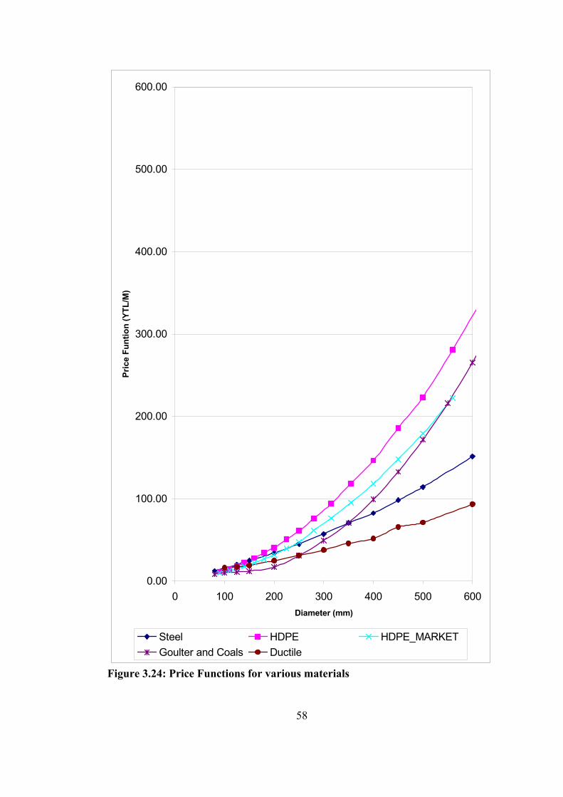
58
0.00
100.00
200.00
300.00
400.00
500.00
600.00
0 100 200 300 400 500 600Diameter (mm)
Pric
e Fu
ntio
n (Y
TL/M
)
Steel HDPE HDPE_MARKETGoulter and Coals Ductile
Figure 3.24: Price Functions for various materials

59
Thus, only items that directly affect the cost of pipe laying are included and price
function of EPA is not used in optimization studies.
3.5.4 Loading Patterns and Pressure Constraints
A set of flow outputs or inputs at the nodes is defined as the loading pattern. The
loading pattern that should govern the design of a water distribution system is not a
definite phenomenon. Whether the system should be designed considering the most
critical instant which occurs rarely during its service time or it should be designed
considering average day conditions which frequently occurs is questionable. The
system can be designed considering the peak hour demands. Alternatively, it can be
designed considering a huge fire within the network. A system designed with these
loadings will have large diameters. However, normal day demands of a system are
much lower than these loadings. Having lower demands in large pipes will cause
reduction of velocity, which in turns results in low quality water. As the velocity
decreases, the microscopic particles within the water tend to settle and ruin the
quality of water. On the other hand, if a system is designed considering average day
demands, the system capacity will not be sufficient against extreme events such as
fires. No one can take the responsibility of human loss due to insufficient pressures at
fire hydrants during a huge fire. Consequently, a system should be designed in such a
way that it should be capable of meeting all of the above criteria.
A guideline for this problem has been given by Walski (1995). He suggested using
the following demand patterns in accordance with the aim of design:
Master Planning: Master planning is done to determine the size and installation date
of major capital projects for a water distribution system. In this type, pipe sizing is
almost completely controlled by the magnitude and location of future municipal and
industrial water use. Because the sizes of larger pipes (>400mm) are generally
controlled by daily demands, not fireflows, sizing has to be checked against peak-
hour or peak day usage. The minimum pressure that must be met needs to be set

60
higher than 140 kpa (20psi). The sizes selected in master planning shall not be
regarded as final decisions, but rather as rough estimates of the best size if all of the
assumptions made in the master planning prove to be true.
Preliminary Engineering for Transmission Mains: During master planning, routes
are approximate, which should be studied in detail during preliminary design. Laying
pipe in cleared land is much less expensive than in congested urban centers with
many buried utilities. Piping decisions are often based on such cost differences.
Additionally, during master planning, the area corresponding to a model node can be
fairly large. In preliminary design, this changes because the location of water users
can be refined further. More importantly, the locations of connections between large
transmission lines and smaller neighborhood distribution pipes must now be
precisely determined. For small distribution components, the probability of an outage
occurring concurrently with the design fire demand is very low, so the system can be
modeled as if all the pipes are in service. In case of large transmission mains, the
probability of the peak demand occurring concurrently with the outage of a system
component is much larger, and the effect of such an outage must be considered in
pipe sizing.
Subdivision development: When land is subdivided for residential development,
industrial parks, shopping malls, the problem is significantly different from master
planning and preliminary design. The sizing is almost completely controlled by fire
flow requirements and most pipes will be of minimum diameter.
In WADISO, the system design is performed considering steady state analysis. The
designer can assign up to five different loading patterns. Different loading patterns
can include variations in
1. Outputs at one or more nodes
2. Minimum pressure requirements at one or more nodes
3. Different specifications for pump operation, including efficiency and the
percentage of time it may run under certain loading patterns.

61
Among the specified patterns, one may be the peak flow expected during a normal
day, while another may represent the necessary flows necessary to fight a fire at
specific node(s). The program will consider all specified loading patterns and will
determine the pipe sizes that are capable of handling flows and minimum pressures
for all patterns. In addition to flow outputs, different minimum pressure patterns can
be specified for different loading patterns.
Pressure constraints are the minimum pressures defined by the designer to be met or
exceeded in the final solution at as many nodes as desired, for each of the loading
patterns under investigation. Pressure constraints are dependant on the aim of the
loading pattern. For example, minimum pressure of 25~30m head at all nodes, which
corresponds to feeding approximately to a 3-storey building without extra pumping,
is the general design criteria for peak hour and maximum day demand while 30m is
required at a specific node at which fire fighting takes place and only 10m head is
sufficient at the remaining nodes.
3.5.5 Pump and Tank Inclusion
Optimization algorithm within WADISO allows designer to include pumping costs.
As the result of the pressure distribution, the flow rates through the pump and the
pump head are obtained. This permits the computation of pumping cost if the
percentage of time the pump is running at this operation point is specified. As
discussed, it is possible to specify several loading patterns, each with its own
percentage of time. The program will then calculate and accumulate the present value
of the pumping cost and add it to the pipe cost.
The pumping cost is calculated from the following equations:
µρgQHkWPower =)( (3.10)
where ρ= mass density of liquid
g=gravitational acceleration (9,81m/s2)

62
Q= pumping flow rate (m3/s)
H= Pump head (m)
µ= Pump efficiency
The user defines the cost per kW and the program calculates the overall pumping
cost considering the percentage time of running in the design life.
In the optimization routine of employed by WADISO, the cost of water storage (i.e.
tanks and reservoirs) can be included in the optimization, in addition to pipe cost and
energy cost. Similar to pumping cost, there exists a trade-off between pipe cost and
storage cost. In general, smaller, less expensive pipe size combinations will require
larger, more expensive storage tanks for balancing peaks in the water demand
whereas larger diameters will increase the pipe cost and also results in low quality
water.
To calculate tank cost, similar to pipe price function, user defines price function that
describes the cost per unit storage with up to 25 volumes sizes. The program
enumerates all of the possible combinations of tank sizes in connection with pipe
combinations.
3.5.6 Pareto Optimal Solutions
The optimal solution proposed by any algorithm may be unfeasible for a number of
reasons, due to political decisions, reduced reliability etc. In addition, non-optimal
(but near-optimal) solutions may display attributes that make these solutions
attractive. For instance, a solution may display a slightly higher than optimal cost,
but it may provide significantly better pressure characteristics than the optimal
solution, though both solutions meet the pressure requirement. Another solution may
violate the pressure requirement by a small amount, yet it may provide for substantial
cost savings. It may then be of interest to invest in a slightly more expensive solution
or sacrifice somewhat on the required pressure (Walski et al., 1990)
63
WADISO uses partial enumeration technique, namely it tries all of the possible
combinations under certain restrictions explained above. During these trials, user can
give such parameters to the program that it can keep some more combinations that
are not optimum, but near optimum. With the aid of this, WADISO allows one to
generate such a set of alternative non-inferior solutions that have the property of
being Pareto Optimal.
A Pareto optimal solution is one in which one of the measures of optimality cannot
be improved without making another measure worse. For the problem of pipe
network optimization specifically, there are two cases:
1. For solutions that meet pressure constraints and are within the cost
tolerance, a solution is Pareto optimal (non-inferior) if there is no other
solution that can give equal or greater pressure at lower cost.
2. For solutions that do not meet the pressure constraints but are within the
pressure tolerance, a solution is Pareto optimal (non-inferior) if there is no
other solution that can give equal or greater pressure at lower cost.
There can be many Pareto optimal solutions for a specific network problem.
64
CHAPTER 4
CASE STUDY 4.1 AIM OF THE STUDY
The aim of this study is to illustrate use of an optimization technique, i.e. WADISO,
on an already constructed real world network and show the discrepancies between
the traditional network design and design using an optimization software. The case
study area is North 8 (N8) pressure zone of Ankara Municipality Water Distribution
System (Merzi et al. 1998a, 1998b). Optimization software is WADISO (Water
Distribution Network Analysis), which uses partial enumeration technique developed
by Gessler (1985).
4.2 WATER DISTRIBUTION SYSTEM OF ANKARA
Ankara being the capital and second largest city of Turkey has a population of
3.203.362 according to year 2000 census (DİE – State Statistical Institute).
Considering that its population was 2.583.963 in year 1990, there has been 21,48 %
increase in the last 10 years. This great development indicates that there is a
migration from rural areas to Ankara city center and in the future, this will continue.
According to ASKİ (Ankara Water and Sewage Management), water consumption
per capita is approximately 250 lt/day/capita as per year 2000 data. As water supply
is one of the primary missions of the state institutions, Ankara has a relatively large
water supply and distribution system.
65
Ankara water supply and distribution system is taking raw water from the following
dams:
• Kurtboğazı Dam
• Çamlıdere Dam
• Akyar Dam
• Eğrekkaya Dam
• Bayındır Dam (via pumping)
• Çubuk-2 Dam
The main Water Treatment Plant is located in İvedik, which is composed of four
units each having a capacity of 564.000 m3/day. With this capacity, İvedik treatment
plant is within the top ten treatment plants among European countries. Pre-stressed
concrete main lines with diameters equal to 2000mm coming from Kurtboğazı Dam
and Çamlıdere Dam are carrying raw water to this plant. Two other treatment plants
are Bayındır Treatment Plant for Bayındır main line with 30.000-m3/day capacity
and Pursaklar Treatment Plant for Çubuk main line with 75.000 m3/day.
Water distribution system of Ankara is divided into five main pressure zones:
• Central and Western Supply Zone (e.g. Sincan, Etimesgut, Eryaman)
• Northern Supply Zone (e.g. Keçiören)
• Eastern and Southeastern Supply Zone (e.g.Mamak)
• Southern Supply Zone (e.g. Çankaya)
• Southwestern Supply Zone (e.g. Çayyolu, Ümitköy)
Each main pressure zone is composed of several pressure zones by approximately
40-50m elevation intervals. Central and Western Zone is divided into two pressure
zones as C2 and W2. Northern Supply Zone is divided into eight pressure zones
named N3-N10. Eastern and Southeastern Zone has seven pressure zones at east
named E3-E9 and four at southeast named SE3-SE7. Southern Supply Zone has ten

66
pressure zones named S3-S12 and South Western Supply Zone has four zones named
SW3-SW6 (Figure 4.1) (YILDIZ, 2002).
The Northern Zone, the study area is located, takes water from P1 Main Pumping
Station. P1 is the main pumping station that takes water directly from İvedik
Treatment Station and distributes to other sub-zones. Water from P1 main station is
carried to P2, which is the main pumping station of Northern Zone. (Figure 4.2, 4.3).
4.3 STUDY AREA
4.3.1 N8 Pressure Zone
The study area, N8 Pressure Zone (Figure 4.3) is located at the end of north line of
Ankara Municipal Water Supply System. In administrative terms, it is located in
Yenimahalle and Keçiören counties. There are four districts fed from N8 sub-
pressure zone, which are Yayla, Sancaktepe, Şehit Kubilay districts of Keçiören and
Çiğdemtepe district of Yenimahalle. There are approximately 25.000 people living in
these districts.
N8 pressure zone is selected for case study due to its simple network system as well
as its relatively homogenous residents. The pressure zone is composed of one
pumping station P23, one main line going from pump to tank, T53, and another main
line feeding northern zone. This configuration is the ideal one for any research
purposes. The water consumption within the zone is mostly residential type. There
are almost no significant industrial or commercial activities located within the
boundaries of N8. The socioeconomic level of the residents can be accepted as low
income; they are distributed uniformly in the pressure zone (Eker, 1998).
Additionally, with the aid of SCADA system installed in the pump station and the
tank, real water consumption values are readily available. With the help of
homogeneity of the system and the data from SCADA, it is possible to determine
nodal demands with negligible error.

67
Figure 4.1: Water Distribution System of Ankara
67
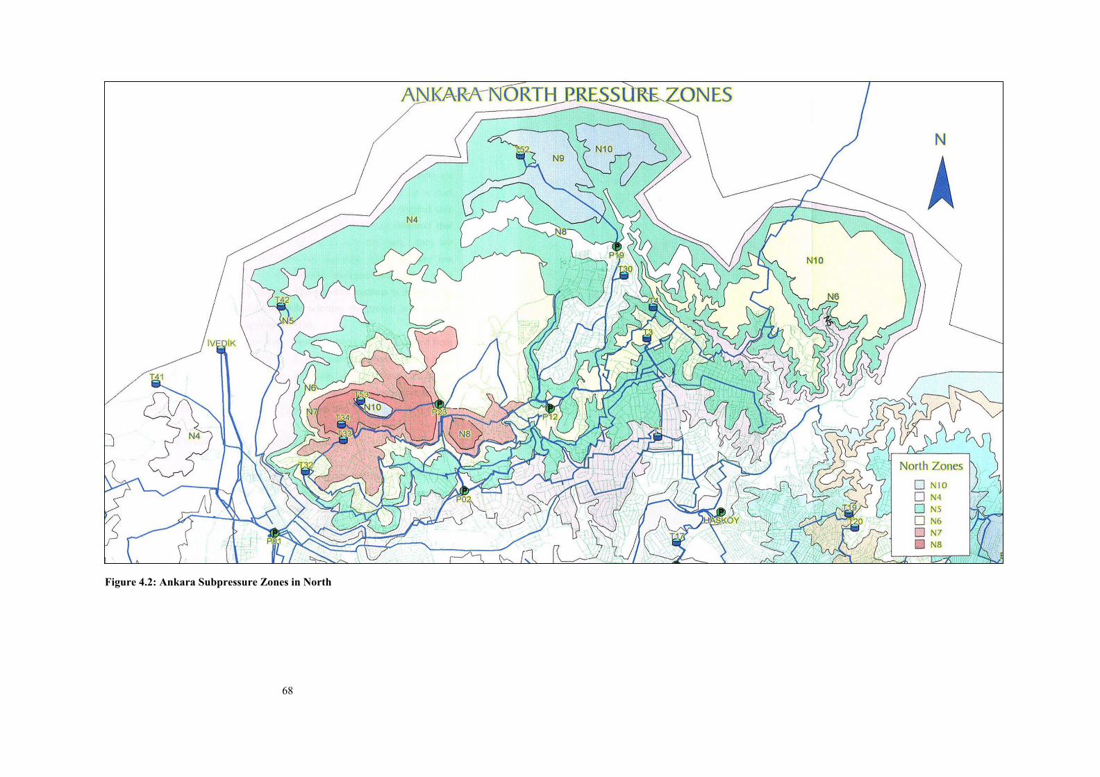
68
Figure 4.2: Ankara Subpressure Zones in North
68

PUM
P (P
23)
TAN
K (T
53)
Figu
re 4
.3: N
8 Pr
essu
re Z
one
70

71
4.4. HYDRAULIC MODEL
4.4.1. Layout of the Pipes in N8 Pressure Zone
The layout of the existing system of N8 Pressure Zone is gathered from ASKİ,
including all characteristics of the pipes, nodes, tank and the pump such as diameters,
elevations, tank dimensions, pump curves etc.
4.4.2. Nodal Demands
In order to determine nodal demands to assign at the nodes of the study area, namely
N8 Pressure Zone, previous studies on this area are searched and nodal demands of
August 16, 2001, which is one of the critical months of the year due to high
temperature and consequently high water usage, are selected, and nodal demands are
assigned. Design load is Qpeak=115,75 lt/s.
4.4.3. Analysis of Existing System
All the system data are entered into WATERCAD 6.0 and the existing system is
analyzed. As seen from Table 4.1 and Figure 4.4, there are some nodes (25 out of
337) with pressure values below 30m, which is the minimum design criteria as stated
in Chapter 2. However, because they are not too low, i.e. around 20, it can be
concluded that in the design stage, these nodes might have been sacrificed for the
good of the area from cost point of view and no further improvements to increase the
pressure values at the said locations were taken.
Further to above, it is observed that the main problem of existing system is not only
the low pressure at specific locations, but also the low velocity in the pipes around
almost the whole system. The minimum flow velocity in the pipes should not be less
than 0,5 m/s to avoid poor water quality. Unfortunately, analysis revealed that the
velocity in the pipes within N8 Zone is too low, where 0,07 m/s is the average
velocity.

72
Table 4.1: Nodes with pressure values below 30m.
Label Elevation (m) Base Flow (l/s) Pressure (m H2O)
J-296 1,142.08 0.0699 12.339 J-289 1,136.56 0.174 17.131 J-270 1,133.79 0.5172 19.842 J-295 1,133.40 0.6408 21.001 J-271 1,132.42 0.3225 21.199 J-274 1,130.71 0.452 22.915 J-249 1,130.26 0.3675 23.357 J-250 1,129.48 0.2914 24.13 J-319 1,128.55 0.2259 25.082 J-269 1,128.46 0.3448 25.164 J-314 1,127.59 0.3537 26.018 J-315 1,127.38 0.3032 26.244 J-251 1,126.41 0.2925 27.192 J-198 1,126.76 0.2532 27.559 J-207 1,125.73 0.2155 28.645 J-291 1,125.02 0.0563 28.687 J-272 1,124.63 0.3963 28.969 J-294 1,125.31 0.0721 29.075 J-252 1,124.43 0.2913 29.166 J-256 1,124.17 0.1925 29.425 J-199 1,124.87 0.4785 29.488 J-206 1,124.78 0.2026 29.586 J-204 1,124.58 0.1991 29.781 J-205 1,124.58 0.1346 29.783 J-208 1,124.55 0.1274 29.829

Fi
gure
4.4
: Pre
ssur
e D
istr
ibut
ion
in E
xist
ing
Syst
em
73
Tan
k (T
53)
Pum
p (P
23)

74
4.4.4. Optimization of the Existing System
4.4.4.1. Grouping of the Pipes Considering Whole System
The very first step of optimization of the system by use of WADISO is the grouping
of pipes, namely, selecting similar pipes and assigning one pipe size to them.
Considering the principals of grouping given in Chapter 3.5.1 (serial pipes, parallel
pipes, pipes feeding same node etc), existing N8 pressure zone is analyzed.
Obviously, the main line going from pump P23 to tank T53 forms Group 1 and while
the other main line feeding northern area forms Group 2. Similarly, main lines within
sub-pressure zones forms separate groups. After grouping of the main lines,
branching lines are studied and pipes going in parallel in the same sub-pressure zone
form separate groups. In short, 72 No. groups are obtained for use in the
optimization.
As stated in Chapter 2, the aim of grouping pipes is to reduce computation time.
However, with the aid of researchers from WADISO S.A., it is concluded that if the
system would be run with 72 groups with each having 3 or more candidate pipe
sizes, it would take almost 1030 years, almost infinity, to finish the computations with
today’s desktop computers. Consequently, the system has to be skeletonized in order
to decrease pipe groups.
4.4.4.2 Skeletonization of the Existing System
To skeletonize a system, such as equivalent parallel pipes by changing the remaining
diameters and/or friction coefficients will result in pipe diameters having values
other than commercially available ones such as 113mm. Because the aim of the
skeletonization in this thesis study is only to reduce number of pipe groups to allow
further computations of optimization, starting computations with diameters 113mm
will be not feasible.
Then, the main lines of the existing system having diameter equal to or greater than
150mm are identified and kept in the system. The resulting layout is given in Figure
75
4.5, yellow pipes being the pipes that should be removed (i.e. not included in
optimization).
As seen from Figure 4.5, the system is not a looped network which threatens the
results of optimization. In order to provide loops, some pipes with smaller diameters
are also introduced (Green pipes in Figure 4.6) and finally the layout of skeletonized
system is obtained as shown in Figure 4.6.
After obtaining the layout of the skeletonized system, it is time to distribute nodal
demands of collapsing pipes. To perform this operation following steps are applied:
. Dead end pipes are identified and the nodal demands at the dead ends are
carried to the other ends. (Figure 4.7)
. If a node is not on a path that is directly branching from the skeletonized
system, it is transferred into the in reverse proportion of the connecting pipes. (Figure
4.8)
. If a node is on a path that is directly branching from the skeletonized
system, it is transferred into the branching node. (Figure 4.9)
Completing all these steps for the entire network, skeletonized system with
transferred nodal demands at each node is obtained, by which the total demand of the
main system is equal to that of skeletonized system.

Fi
gure
4.5
: Pip
es w
ith d
iam
eter
equ
al o
r gr
eate
r th
an 1
50m
m.
76
Tan
k (T
53)
Pum
p (P
23)

Fi
gure
4.6
: Ske
leto
nize
d L
ayou
t of N
8 Pr
essu
re Z
one
77
Tan
k (T
53)
Pum
p (P
23)

78
Deman
d is t
ransfe
rred
to thi
s nod
e
Dead End Node
Figure 4.7: Demand Transfer of a Dead End Node
Figure 4.8: Demand Transfer of a Node That is NOT ON THE PATH
Skeletonized System
Collapsing Nodes
Collapsing Nodes
Dem
and
is tr
ansf
erre
d
to th
is n
ode
Collapsing Node
Demand is transferred
to this node
Skeletonized System

79
Dem
and
is tra
nsfe
rred
to th
is no
de
SkeletonizedSystem
Skeletonized System
Collapsing Nodes
Collapsing Nodes
Deman
d is t
ransfe
rred
to thi
s nod
e
Collapsing Node
Collapsing Node
Figure 4.9: Demand Transfer of a Node That is ON THE PATH
4.4.4.3 Grouping of Pipes for the Skeletonized Network
The grouping of pipes within skeletonized network is initiated by grouping of the
main lines forming individual groups. The result is seven groups. As discussed
previously, in order to reduce computation time, number of pipe groups should not
exceed 15, which is a constraint resulting from WADISO. Thus, remaining pipes, i.e.
pipes with diameters equal to either 125mm or 100mm, are studied very carefully in
order to find the most critical ones. After this, remaining eight Groups are formed
and first step of optimization is completed (Figure 4.10, Table 4.2). As can be noted
from Figure 4.10, there are some pipes that are not introduced in the optimization
process (yellow ones, mostly with diameter equal to 125mm or 100mm); they are not
contained in any group and their diameters remain unchanged. However, since those
remaining pipes have already smaller diameters, this does not have a significant
effect on the results.

Figu
re 4
.10:
Pip
e G
roup
s of S
kele
toni
zed
Net
wor
k
80
Tan
k (T
53)
Pum
p (P
23)

Tab
le 4
.2: P
ipe
Gro
ups o
f Ske
leto
nize
d N
etw
ork
GR
OU
P 1
GR
OU
P 2
GR
OU
P 3
GR
OU
P 4
GR
OU
P 5
GR
OU
P 6
GR
OU
P 7
GR
OU
P 8
GR
OU
P 9
GR
OU
P 10
G
RO
UP
11
GR
OU
P 12
G
RO
UP
13
GR
OU
P 14
G
RO
UP
15
2 12
1
251
348
377
379
301
111
102
237
201
192
462
442
3 15
12
5 27
2 34
9 38
2 38
4 30
2 14
9 10
3 24
0 20
2 19
3 46
3 44
3 4
17
126
273
354
391
424
303
152
104
249
212
194
464
453
10
30
127
274
358
435
431
304
153
105
263
215
195
465
454
11
31
128
279
367
436
432
305
154
137
266
216
196
466
460
42
15
8 29
9 36
8 43
9 43
3 30
6 15
6 16
6
261
205
470
461
43
17
2 31
8 37
1 44
0 43
8 30
7 15
7
26
2 20
6
46
174
321
372
44
1
159
265
50
177
326
376
16
0
55
291
457
387
16
1
56
292
467
388
16
2
59
308
469
392
17
1
61
309
39
6
173
65
41
2
399
66
48
0
416
74
48
1
418
75
99
8
419
82
42
0
88
427
92
42
8
PIPES IN THE GROUP
93
81
82
4.4.4.4. Candidate Pipe Sizes
After grouping of pipes, it is time to assign candidate pipe sizes for every individual
group. Similar to number of groups, number of candidate pipe size for a group has
also significant effect on the computation time, the more the candidate sizes the more
computation time. Thus, every group has to be studied very carefully and
unnecessary candidate sizes should be eliminated at the beginning.
For the first run, it is decided to give three candidate pipe sizes for each group, one
being the existing diameter, one size higher and one size smaller. As an example, the
main line going from pump to tank with existing diameter equal to 500mm that also
forms Group No 3, is assigned candidate pipes sizes of 400mm, 500mm, and
600mm. The aim of this procedure is to determine whether the system is over-
designed or under-designed. After determination of this, more pipe sizes are assigned
in order to find the optimum pipe size for each group (Refer to Section 3.5.2).
Table 4.3 shows candidate pipe sizes for each group for the first run to determine if
the system is over-designed or under-designed. Table 4.4 shows the candidate pipe
sizes for the final run.
4.4.4.5. Price Functions
The main objective of optimization is being to assign the most economical diameters
for every pipe; one of the crucial points of the whole process is to assign correct
price functions to each diameter. A small error on this step may ruin the whole result.
As an example, if the price function of 200mm pipe is assigned very close to 100mm
pipe, the software will assign 200mm. Then, the result will be most probably an
over-designed system with pipes having 200mm diameter where 100mm would be
sufficient. As a summary, the price functions should reflect the real world situation
as much as possible.

Tab
le 4
.3: C
andi
date
Pip
e Si
zes t
o de
term
ine
if th
e sy
stem
is o
ver-
desi
gned
or
unde
r-de
sign
ed.
G
R 1
G
R 2
G
R 3
G
R 4
G
R 5
G
R 6
G
R 7
G
R 8
G
R 9
G
R 1
0 G
R 1
1 G
R 1
2 G
R 1
3 G
R 1
4 G
R 1
5
250
150
400
200
150
100
125
125
125
150
150
125
150
125
150
300
200
500
250
200
125
150
150
150
200
200
150
200
150
200
CANDIDATE PIPE SIZES
350
250
600
300
250
150
200
200
200
250
250
200
250
200
250
EXISTING PIPE SIZES
300
200
500
250
200
125
150
150
150
200
200
150
200
150
200
83

Tab
le 4
.4: C
andi
date
Pip
e Si
zes f
or th
e fin
al r
un
G
R 1
G
R 2
G
R 3
G
R 4
G
R 5
G
R 6
G
R 7
G
R 8
G
R 9
G
R 1
0 G
R 1
1 G
R 1
2 G
R 1
3 G
R 1
4 G
R 1
5
200
125
200
125
100
100
125
125
125
150
150
100
150
125
150
150
100
250
150
125
125
150
150
150
200
200
125
200
150
200
125
30
0 20
0 15
0
100
100
100
100
100
150
100
100
100
CANDIDATE PIPE SIZES
100
40
0 25
0
EXISTING PIPE SIZES
300
200
500
250
200
125
150
150
150
200
200
150
200
150
200
84
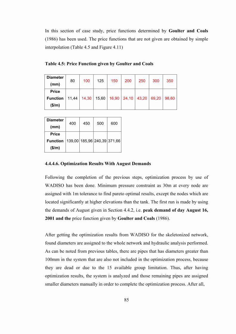
85
In this section of case study, price functions determined by Goulter and Coals
(1986) has been used. The price functions that are not given are obtained by simple
interpolation (Table 4.5 and Figure 4.11)
Table 4.5: Price Function given by Goulter and Coals
Diameter (mm)
80 100 125 150 200 250 300 350
Price Function
($/m) 11,44 14,30 15,60 16,90 24,10 43,20 69,20 98,60
Diameter (mm)
400 450 500 600
Price Function
($/m) 139,00 185,96 240,39 371,66
4.4.4.6. Optimization Results With August Demands
Following the completion of the previous steps, optimization process by use of
WADISO has been done. Minimum pressure constraint as 30m at every node are
assigned with 1m tolerance to find pareto optimal results, except the nodes which are
located significantly at higher elevations than the tank. The first run is made by using
the demands of August given in Section 4.4.2, i.e. peak demand of day August 16,
2001 and the price function given by Goulter and Coals (1986).
After getting the optimization results from WADISO for the skeletonized network,
found diameters are assigned to the whole network and hydraulic analysis performed.
As can be noted from previous tables, there are pipes that has diameters greater than
100mm in the system that are also not included in the optimization process, because
they are dead or due to the 15 available group limitation. Thus, after having
optimization results, the system is analyzed and those remaining pipes are assigned
smaller diameters manually in order to complete the optimization process. After all,

86
Price Function Graph
0.00
50.00
100.00
150.00
200.00
250.00
300.00
350.00
400.00
0 100 200 300 400 500 600
Diameter (mm)
Pric
e Fu
ctio
n ($
/m)
Price Function by Goulter & Coals Derived Functions
Figure 4.11: Graphical Interpretation of Price Function

87
optimized system is obtained with the pressure values below 30m as tabulated in
Table 4.6. As can be observed, there are some nodes that have pressure values above
30m in the existing system but have less than 30m in the optimized system. The
reason for this is that, in order to obtain the most economical system, pressure
constraint is relaxed for this small number of nodes. Nodes designated as “N/A” in
Table 4.6 are the ones that are not included in optimization process.
The results show that the system is over-designed with the demands of August. The
cost of existing system is 939.630,13 YTL (with ductile price function) while the
pressure constraints can be satisfied with a system having total cost of
542.297,52YTL (with price function given by Goulter and Coals). The diameters
of main lines are reduced to almost half of the existing ones. Most of the diameters of
pipes are assigned as 100mm, which is the smallest diameter pipe that is allowed by
the Municipality. Optimum pipe diameters for every group is given is Table 4.7.
Because the pipe diameters are decreased, some improvement on velocity also
gained. The result found by optimization is not a surprise since the demands are very
low due to the socio-economical nature of the pressure zone.
4.4.4.7. Optimization Results with Demands Including Pipe Leakages and Year
2020
Today’s N8 pressure zone design was completed and implemented in 1990s.
However, in 1998, thesis study of İlker EKER (1998) showed that there were
leakages in N8 zone and further studies done with cooperation of METU and ASKİ
revealed the leakage causes (Merzi et al 1998a, 1998b). Consequently, it was
revealed that the real demands of N8 zone are lower than the ones used in the
previous design stage. Daily demand curve of N8 before the said studies is given in
Figure 4.12.
Furthermore, as discussed in Chapter 2, the system designs are made considering
future demands, normally considering 20~25 years later. Considering this situation,
the demands are further increased according to forecasted total demand of year 2020.
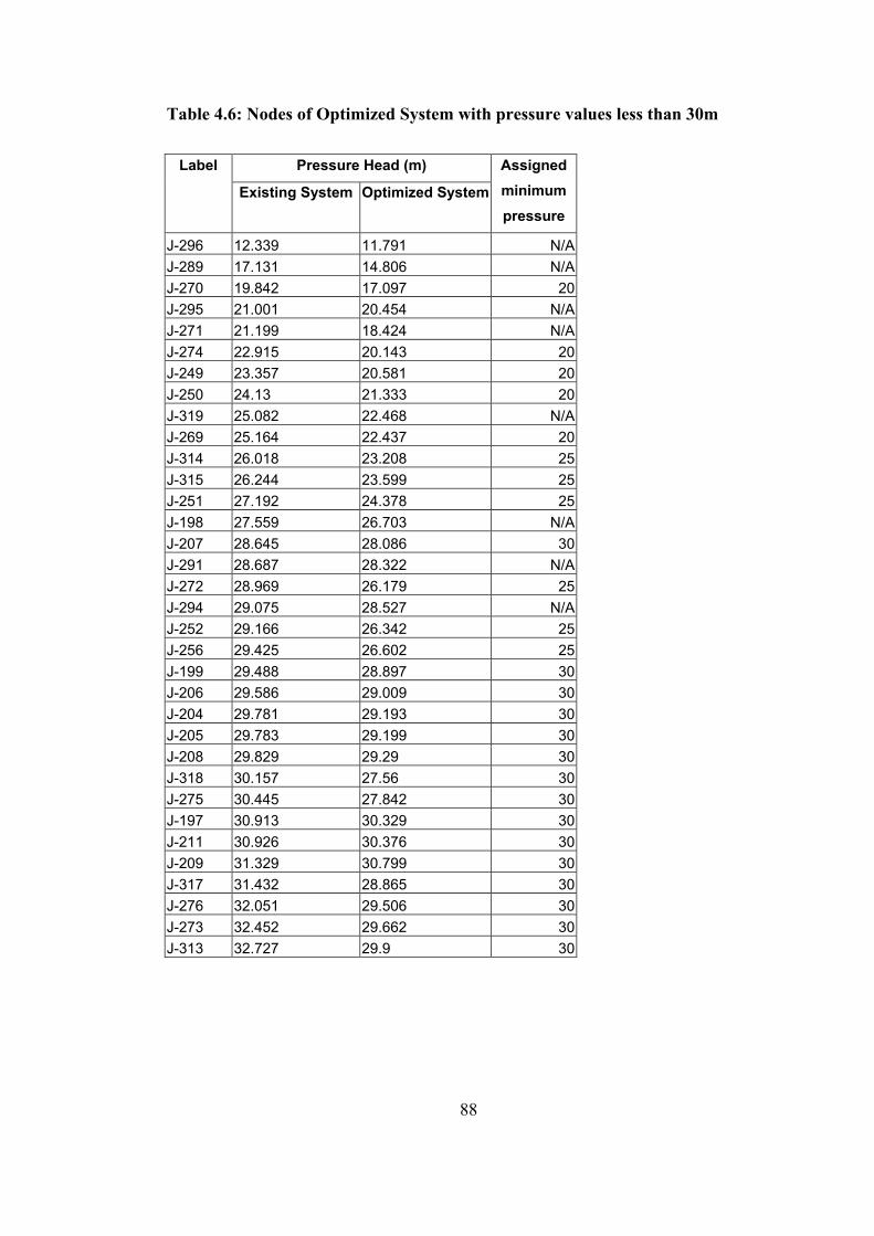
88
Table 4.6: Nodes of Optimized System with pressure values less than 30m
Pressure Head (m) Label
Existing System Optimized System
Assigned minimum pressure
J-296 12.339 11.791 N/AJ-289 17.131 14.806 N/AJ-270 19.842 17.097 20J-295 21.001 20.454 N/AJ-271 21.199 18.424 N/AJ-274 22.915 20.143 20J-249 23.357 20.581 20J-250 24.13 21.333 20J-319 25.082 22.468 N/AJ-269 25.164 22.437 20J-314 26.018 23.208 25J-315 26.244 23.599 25J-251 27.192 24.378 25J-198 27.559 26.703 N/AJ-207 28.645 28.086 30J-291 28.687 28.322 N/AJ-272 28.969 26.179 25J-294 29.075 28.527 N/AJ-252 29.166 26.342 25J-256 29.425 26.602 25J-199 29.488 28.897 30J-206 29.586 29.009 30J-204 29.781 29.193 30J-205 29.783 29.199 30J-208 29.829 29.29 30J-318 30.157 27.56 30J-275 30.445 27.842 30J-197 30.913 30.329 30J-211 30.926 30.376 30J-209 31.329 30.799 30J-317 31.432 28.865 30J-276 32.051 29.506 30J-273 32.452 29.662 30J-313 32.727 29.9 30

Tab
le 4
.7: O
ptim
um D
iam
eter
s with
Aug
ust D
eman
ds
G
R 1
G
R 2
G
R 3
G
R 4
G
R 5
G
R 6
G
R 7
G
R 8
G
R 9
G
R 1
0 G
R 1
1 G
R 1
2 G
R 1
3 G
R 1
4 G
R 1
5
EXIS
TIN
G
DIA
MET
ERS
300,
00
200,
00 5
00,0
0 25
0,00
200
,00
125,
00 1
50,0
0 15
0,00
15
0,00
20
0,00
20
0,00
150
,00
200,
00 1
50,0
0 20
0,00
CA
ND
IDAT
E D
IAM
ETER
S (m
m)
200
125
200
125
100
100
125
125
125
150
150
100
150
125
150
15
0 10
0 25
0 15
0 12
5 12
5 15
0 15
0 15
0 20
0 20
0 12
5 20
0 15
0 20
0
12
5
300
200
150
10
0 10
0 10
0 10
0 10
0 15
0 10
0 10
0 10
0
10
0
400
250
OPT
IMU
M
DIA
MET
ERS
(mm
) 15
0 10
0 30
0 20
0 12
5 10
0 10
0 10
0 10
0 10
0 10
0 10
0 10
0 12
5 10
0
89

Figu
re 4
.12:
Dai
ly D
eman
d C
urve
of N
8 In
clud
ing
Lea
kage
s
90

91
From Figure 4.12, peak loading is read as Qpeak=330,4 m3/h (91,77 lt/s) and night
loading as 64,6 m3/h (17,94 lt/s).
Demand Forecast for Year 2020
Demand projection for year 2020 is performed by use of the following formula (İller
Bankası, 1998):
knownYear
know kFF−
+=2020
2020 100/1* (4.1)
where F is the total demand, k is a coefficient.
In this equation, maximum value of k can only be 3.
In order to find the maximum available design in year 2020, it is decided to take k as
maximum, i.e. k=3.
Consequently for peak loading, Qpeak ,
sltQF peak /13,181100/31*77,9119972020
2020 ==>+=−
Similarly for night loading, Qnight,
sltQF night /417,35100/31*94,1719972020
2020 ==>+=−
For fire loading, , Qfire , 15lt/s fire flow need is assigned to two neighboring critical
nodes, i.e. nodes with pressure values below 30m, during Qpeak. These nodes are
selected as Node 270 and Node 271.
Additionally, as discussed in Section 3.5.3, the price function can also be very
significant. To demonstrate this in this section, the same system is optimized using
various price functions with three loading cases of Year 2020, but keeping all the
other variables unchanged, i.e. groups. At every optimization trial, Peak Loading
(Qpeak), Fire Loading (Qfire) and Night Loading (Qnight) are assigned simultaneously to

92
the software so that it can decide the critical one. As pressure constraints, following
are assigned for every loading case as given in Table 4.8.
Table 4.8: Pressure Constraints for Optimization
Loading Pressure Constraint
Peak loading
30m minimum head at every node, except the ones
located at significantly higher elevations than the tank
Fire Loading 15m minimum head at every node
Night Loading
30m minimum head at every node, except the ones
located at significantly higher elevations than the tank
Optimization With Various Price Functions: Using built price functions in Section
3.5.3.1 and Hazen-Williams coefficient based on material type; series of optimization
studies are performed for three loading cases (Peak, fire and night loading). Total
cost of N8 pressure zone with the optimum diameters, which are found based on
various price functions, are given in Table 4.9. As it is observed from Table 4.9, the
cost of the same system varies based on the material used. As the result of these
studies, optimum pipe diameters depending on price functions are tabulated in Table
4.10. However, on the contrary to expectations, there are no significant development
in pressures regardless of the pipe material used and the cost of total system, namely,
pressures almost remain same whatever material is used and the problematic nodes
remain almost same with all the system configurations (Figures 4.13~4.27,
APPENDIX A).

93
Table 4.9: Total System Cost Optimized With Various Price Functions
PRICE FUNCTION TOTAL COST (YTL)
HDPE Price Function with DSI Prices 920.425,91
HDPE Price Function with Market Prices 758.148,59
Steel Price Function with DSI Prices 935.841,50
Ductile Price Function with Market Prices 832.375,39
COST OF EXISTING SYSTEM (with ductile price function) 939.630,13

T
able
4.1
0: O
ptim
um p
ipe
diam
eter
s dep
endi
ng o
n pr
ice
func
tions
OPT
IMU
M
DIA
MET
ERS
(mm
) G
R 1
G
R 2
G
R 3
G
R 4
G
R 5
G
R 6
G
R 7
G
R 8
G
R 9
G
R 1
0 G
R 1
1 G
R 1
2 G
R 1
3 G
R 1
4 G
R 1
5
STEE
L 20
0 10
0 40
0 30
0 20
0 10
0 12
5 10
0 10
0 10
0 10
0 10
0 10
0 10
0 10
0
DU
CTI
LE
200
100
400
300
200
100
125
100
100
100
100
100
100
100
100
HD
PE_M
AR
KET
16
0 11
0 40
0 25
0 16
0 90
11
0 90
90
90
90
90
90
12
5 18
0
HD
PE_D
SI
160
110
400
250
160
90
110
90
90
90
90
90
90
125
180
EXIS
TIN
G P
IPE
DIA
MET
ERS
300
200
500
250
200
125
150
150
150
200
200
150
200
150
200
94
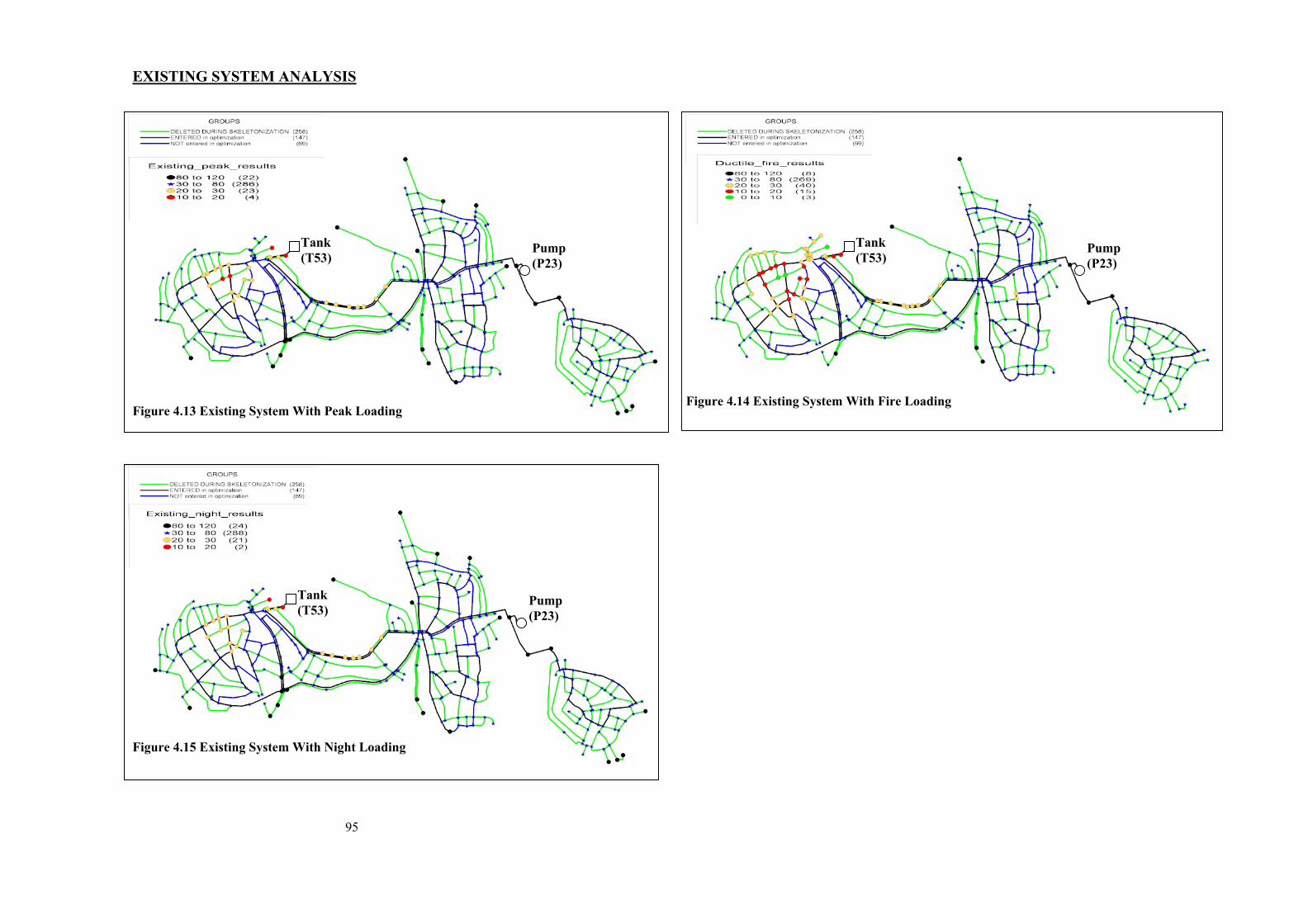
95
EXISTING SYSTEM ANALYSIS
Figure 4.13 Existing System With Peak Loading Figure 4.14 Existing System With Fire Loading
Figure 4.15 Existing System With Night Loading
Tank (T53)
Pump (P23)
Tank (T53)
Pump (P23)
Tank (T53)
Pump (P23)
95

96
RESULTS WITH PEAK DEMANDS
Figure 4.16: System with Ductile (or Steel) Pipes Under Peak Loading Figure 4.17: System with HDPE Pipes (DSI Prices) Under Peak Loading
Figure 4.18: System with HDPE Pipes (Market Prices) Under Peak Loading
Tank (T53)
Pump (P23)
Tank (T53) Pump
(P23)
Tank (T53) Pump
(P23)
96

97
RESULTS WITH FIRE DEMANDS
Figure 4.20: System with HDPE Pipes (DSI Prices) Under Fire Loading
Tank (T53)
Pump (P23) Tank
(T53) Pump (P23)
Figure 4.19: System with Ductile (or Steel) Pipes Under Fire Loading
Tank (T53) Pump
(P23)
Figure 4.21: System with HDPE Pipes (Market Prices) Under Fire Loading
97
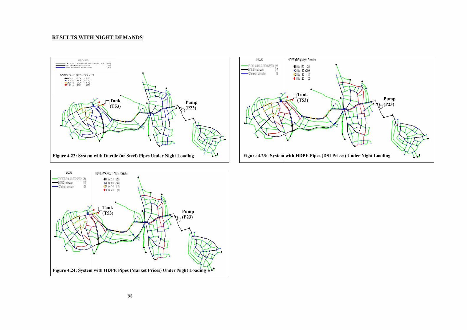
98
RESULTS WITH NIGHT DEMANDS
Figure 4.22: System with Ductile (or Steel) Pipes Under Night Loading Figure 4.23: System with HDPE Pipes (DSI Prices) Under Night Loading
Figure 4.24: System with HDPE Pipes (Market Prices) Under Night Loading
Tank (T53)
Pump (P23)
Tank (T53) Pump
(P23)
Tank (T53) Pump
(P23)
98
99
CHAPTER 5
CONCLUSION AND RECOMMENDATIONS The design of water distribution networks is generally being performed with
traditional (trial-and-error) techniques. This is because most of the techniques are
automatic techniques which do not allow designer to control the steps of process.
However, partial enumeration technique developed by Gessler (1985) is a useful tool
to the designers in which they can control all the steps of the process.
In this study, in order to demonstrate this, a water distribution network is designed by
using Gessler’s (1985) partial enumeration technique with software, WADISO. As
the result of this study, the following conclusions are drawn:
• Partial enumeration technique is a powerful tool that assists designers. With
this technique, designers can select the pipes that should be optimized, the
pipes that should have the same diameters, and the pipes that can be
eliminated or should not be eliminated to secure reliability. Moreover, the
technique provides pareto optimal solutions that offers a different design
which is close to the optimal. The only disadvantage of it is the required
computation time depending on the scale of the design.
• Since partial enumeration technique is based on trial of all possible
combinations one by one considering some rules defined by user, it is
guaranteed that the solution is close to the global minimum, if not itself.
• The price function is very significant in any of the optimization technique.
Correct price functions have to be formed considering special characteristics
of the subject area and the selected pipe materials. There are various pipe

100
materials that can be used in distribution networks such as ductile iron, HDPE
or steel, each having different price functions. However, since each of these
materials has advantageous properties over the others, not only the price
function should be considered, but also factors other than price function
should also be considered.
• It is shown that the cost of pipe fittings can have a significant effect on the
global cost, especially if the system is composed of densely located junctions.
However, no guideline is available to include the cost of pipe fittings in the
price functions.
• Water distribution network of N8 pressure zone is over-designed. Either
smaller diameter pipes should have been installed or staged development
should have been planned.
• Velocities within N8 zone is far below desired values. Because low velocities
in the pipes cause low quality water, aging of pipes occur. In order to satisfy
water quality objective, periodical flushing (extracting water from pipe
hydrants to increase velocities and clean the pipes) should be performed.
Another solution for increasing water quality is to divide N8 pressure zone
further sub-pressure zones.
Furthermore, during the study, conventional pipe laying techniques are considered.
More detailed study can be performed considering other construction techniques
such as pipe jacking, trenchless construction etc.
Although the network designed by use of partial enumeration technique satisfies the
minimum pressure constraints, there is no possibility to control maximum pressures.
Thus, pipe material has to be selected considering pressures. Additionally, there is no
way to satisfy both velocity constraints and pressure constraints with WADISO. The
software does not take velocities into consideration. Future studies on these subjects

101
will definitely improve the capacities of the technique. Finally, with the advances in
the computer technology and development of much more rapid processors in the
future, there will not be any need to follow the steps, which are explained in this
study to reduce computation time, and the software will be capable of enumerating
all possible combinations resulting in the global minimum.

102
REFERENCES
Adıgüzel, R.İ., “ The Optimum Transmission Line Capacity and the Optimum
Operation of Selahattin Saygı Dam”, M.S. Thesis, Middle East Technical University,
March 1976
Akdoğan, T., “Design Of Water Distribution System By Optimization Using Reliability Considerations”, M.S. Thesis, Middle East Technical University, April 2005
Alperovits, E. and Shamir, U. “Design of Optimal Water Distribution Systems”
Water Resources Research, 13(6), 885, 1977
Aygün, E., “Optimization of Hydoelectric Power Production of Sarıyar and
Gökçekaya Reservoirs by Dynamic Programming”, M.S. Thesis, Middle East
Technical University, October 1978
Babbit, H.E. and Doland, J.J., “Water Supply Engineering”, McGraw Hill, New
York, 1931
Bonds, W.R, “Ductile Iron Pipe versus HDPE Pipe”, Ductile Iron Pipe Research
Association, 2000
Clark, R.M., Sivaganesan, M., Selvakumar, A. Sethi, V., “Cost Models for Water
Supply Distribution Systems”, Journal of Water Resources Planning and
Management, September - October, pp.312-321, 2002
Cross, H., “Analysis of Flow in Networks of Conduits or Conductors”, University of
Illinois Engineering Experiment Station Bulletin, 286, 1936

103
Ductile Iron Society, www.ductile.org, last visited on 02.12.2005
Ductile Iron Pipe Research Association, www.dipra.org, last visited on 02.12.2005
İnözü, D., “Optimum Design of Water Distribution Networks”, M.S. Thesis, Middle
East Technical University, October 1977
Eker, İ., “Analysis of Water Distribution Networks Using Information Systems”,
M.S. Thesis, Middle East Technical University, November 1998
Gessler, J. “Optimization of Pipe Networks”, International Symposium on Urban
Hydrology, Hydraulics and Sediment Control, University of Kentucky, Lexington,
1982
Gessler, J., “Pipe Network Optimization by Enumeration”, Proceedings of Specialty
Conference on Computer Applications in Water Resources, American Society of
Civil Engineers, New York, New York pp. 572-581, 1985
Goulter, I. C., Coals, A. V., “Quantitative Approaches to Reliability Assessment in Pipe Networks”, J. Transp. Engrg., ASCE, Vol. 112, No. 3 287-301, 1986.
Goulter, I. C., and Morgan, D.R. “An Integrated Approach to the Layout and Design
of Water Distribution Networks” Civil Engineering Systems, 1985
Fujiwara, O. and Khang, D.B., “A Two-Phase Decomposition Method for Optimal
Design of Looped Water Distribution Networks”, Water Resources Research, 26(4),
539, 1990
İller Bankası, “Regulation for Preparation of Water Distribution Designs for Cities
and Towns” (in Turkish), 1998
Lai, D. and Schaake, J.C., “Linear Programming and Dynamic Programming
Applications to Water Distribution Network Design”, Report 116, Department of
Civil Engineering, MIT, Cambridge, 1969

104
Merzi, N., Şendil, U., Yağız, E., Eker, İ., Poyraz, S., “ Hydraulic Modeling Process
of N8 Pressure Zone of Ankara Water Distribution Network” (in Turkish),
ASKI/METU Joint Education and Training Program, 1st Progress Report, Middle
East Technical University, Ankara, May 1998a
Merzi, N., Şendil, U., Yağız, E., Eker, İ., Poyraz, S., “ Hydraulic Modeling Process
of N8 Pressure Zone of Ankara Water Distribution Network” (in Turkish),
ASKI/METU Joint Education and Training Program, 2nd Progress Report, Middle
East Technical University, Ankara, October 1998b
Özer, S., “Computer Aided Pipeline Design”, M.S. Thesis, Middle East Technical
University, November 1988
Quindry, G.E., Brill, E.D., and Liebman, J.C., “Optimization of Looped Water
Distribution Systems”, J.Environmental Engineering Division ASCE, Vol.107,
No.EE4, 1981
Selmanpakoğlu, M., “Analysis of Water Consumption and Loss and Distribution
System Costs in Turkey”, M.S. Thesis, Middle East Technical University, January
1973,
Sevük, S., Altınbilek, D., “Pipe Network Computations with Computer” (in Turkish),
Ankara, 1976
Sevük, S., Altınbilek, D., “Principles of Design and Solution of Water Distribution
Networks with Computers” (in Turkish), Middle East Technical University Faculty
of Engineering Publications, Ankara, 1977
Soleyman, C., “Optimum Design of Water Distribution Networks”, M.S. Thesis,
Middle East Technical University, May 1976
105
Superlit, www.superlit.com, last visited on 02.12.2005
Tokalak, A.O., “ Road and Pipeline Route Optimization by Discrete Differential
Dynamic Programming”, M.S. Thesis, Middle East Technical University, June 1976
United States Environmental Protection Agency, “Drinking Water Infrastructure
Needs Survey – Second Report to Congress”, Drinking Water Protection Division,
2001
Walski, T.M. “Pipe Network Optimization by Enumeration”, Proceedings of
Specialty Conference on Computer Applications in Water Resources, American
Society of Civil Engineers, New York, New York pp. 558-567, 1985
Walski, T.M. Gessler, J., Sjostrom, J.W., “Water Distribution Simulation and
Sizing”, Lewis Publishers, Michigan, 1990
Walski, T.M., “Optimization and Pipe Sizing Decisions”, Journal of Water
Resources Planning and Management, July – August, pp.340-343, 1995
Walski, T.M., “Relating Design Flow, Pipe Size and Cost”, Essential hydraulics and
hydrology, Haestad Methods, Inc., Waterbury, Conn., 1998
Walski, T., “The Wrong Paradigm – Why Water Distribution Optimization Doesn’t
Work” Journal of Water Resources Planning and Management, July – August,
pp.203-205, 2001
Walski, T.M., Chase, D.V., Savic, D., Gravman, W. M., Beckwith, S., Koelle,E.,
“Advanced Water Distribution Modeling and Management”, Haestad Methods,
Waterburg, 2003
Yıldız, E., “Reliability of Water Distribution Systems”, Middle East Technical
University, 2002

106
APPENDIX - A
Pressure values of Optimum System with various price functions and under three loadings (Peak, Fire and Night Demands of Year 2020)

Tab
le A
- Pr
essu
re v
alue
s of O
ptim
um S
yste
m w
ith v
ario
us p
rice
func
tions
and
und
er th
ree
load
ings
(Pea
k, F
ire
and
Nig
ht D
eman
ds o
f Yea
r 20
20)
Qpe
ak
Qfir
e
Qni
ght
Qpe
ak
Qfir
e
Qni
ght
Qpe
ak
Qfir
e
Qni
ght
Labe
lEl
evat
ion
(m)
Bas
e Fl
ow
(l/s)
Pres
sure
(m
H2O
)B
ase
Flow
(l/
s)
Pres
sure
(m
)B
ase
Flow
(l/
s)Pr
essu
re
(m)
Pres
sure
(m
)Pr
essu
re
(m)
Pres
sure
(m
)Pr
essu
re
(m H
2O)
Pres
sure
(m
H2O
)Pr
essu
re
(m H
2O)
Pres
sure
(m
H2O
)Pr
essu
re
(m H
2O)
Pres
sure
(m
H2O
)
J-1
1.06
1,75
01,
173
91,2
181,
173
90,5
130,
116
93,6
1493
,392
90,9
9493
,408
91,5
2490
,990
93,4
0892
,160
91,9
5592
,937
J-2
1.05
1,77
00,
970
99,5
900,
970
98,8
850,
096
103,
552
103,
302
97,3
4110
3,31
897
,870
97,3
3610
3,31
810
1,90
010
1,69
410
2,89
4J-
31.
061,
250
0,56
089
,267
0,56
088
,562
0,05
594
,079
93,8
1485
,919
93,8
3086
,449
85,9
1593
,830
92,3
1992
,114
93,4
31J-
41.
076,
440
1,56
073
,623
1,56
072
,918
0,15
578
,913
78,6
3969
,658
78,6
5570
,187
69,6
5378
,656
77,0
9376
,887
78,2
71J-
51.
076,
650
1,57
170
,993
1,57
170
,289
0,15
678
,670
78,4
0366
,962
78,4
1167
,492
66,9
5878
,412
76,6
3976
,434
78,0
58J-
61.
090,
980
0,48
356
,359
0,48
355
,654
0,04
864
,364
64,0
9852
,360
64,1
0652
,890
52,3
5664
,106
62,3
2862
,123
63,7
57J-
71.
090,
590
0,28
656
,701
0,28
655
,996
0,02
864
,753
64,4
8752
,711
64,4
9553
,241
52,7
0764
,495
62,7
1662
,510
64,1
46J-
81.
078,
420
0,14
268
,846
0,14
268
,141
0,01
476
,898
76,6
3364
,856
76,6
4065
,386
64,8
5276
,641
74,8
6174
,655
76,2
91J-
91.
085,
450
0,10
064
,398
0,10
063
,694
0,01
069
,918
69,6
4060
,116
69,6
5660
,646
60,1
1269
,656
68,0
6367
,857
69,2
78J-
101.
087,
530
0,29
862
,323
0,29
861
,618
0,02
967
,842
67,5
6458
,041
67,5
8058
,570
58,0
3667
,580
65,9
8765
,782
67,2
03J-
111.
086,
610
0,31
663
,168
0,31
662
,463
0,03
168
,759
68,4
8058
,786
68,4
9659
,316
58,7
8268
,496
66,8
9366
,688
68,1
21J-
121.
086,
120
0,13
363
,255
0,13
362
,550
0,01
369
,243
68,9
6658
,982
68,9
8159
,511
58,9
7768
,981
67,3
7167
,165
68,6
09J-
131.
077,
120
0,13
372
,236
0,13
371
,531
0,01
378
,225
77,9
4867
,963
77,9
6368
,493
67,9
5977
,963
76,3
5276
,146
77,5
91J-
141.
093,
900
1,77
654
,342
1,77
653
,637
0,17
661
,463
61,1
9150
,150
61,2
0250
,680
50,1
4661
,202
59,5
9259
,386
60,8
45J-
151.
086,
610
0,61
861
,589
0,61
860
,884
0,06
168
,738
68,4
6857
,626
68,4
8058
,156
57,6
2268
,480
66,8
4766
,641
68,1
20J-
161.
094,
240
0,61
253
,821
0,61
253
,117
0,06
161
,121
60,8
5149
,744
60,8
6150
,274
49,7
4060
,862
59,2
0959
,003
60,5
05J-
171.
093,
570
1,45
753
,774
1,45
753
,069
0,14
461
,780
61,5
1449
,775
61,5
2150
,305
49,7
7161
,522
59,7
4559
,539
61,1
72J-
181.
090,
200
0,55
757
,050
0,55
756
,345
0,05
565
,142
64,8
7653
,072
64,8
8353
,602
53,0
6864
,884
63,1
0562
,899
64,5
35J-
191.
086,
180
0,54
061
,035
0,54
060
,330
0,05
369
,153
68,8
8857
,061
68,8
9557
,591
57,0
5768
,896
67,1
1366
,907
68,5
47J-
201.
067,
720
0,20
579
,457
0,20
578
,752
0,02
087
,576
87,3
1075
,482
87,3
1876
,012
75,4
7887
,318
85,5
3485
,329
86,9
70J-
211.
086,
710
0,86
960
,506
0,86
959
,801
0,08
668
,624
68,3
5956
,532
68,3
6657
,062
56,5
2868
,367
66,5
8466
,378
68,0
18J-
221.
069,
860
0,38
877
,312
0,38
876
,608
0,03
885
,440
85,1
7573
,336
85,1
8273
,866
73,3
3285
,182
83,3
9183
,185
84,8
34J-
231.
068,
020
0,14
179
,148
0,14
178
,443
0,01
487
,276
87,0
1175
,172
87,0
1875
,702
75,1
6787
,019
85,2
2785
,021
86,6
70J-
241.
102,
870
0,59
844
,393
0,59
843
,688
0,05
952
,497
52,2
3140
,425
52,2
3940
,954
40,4
2052
,239
50,4
6850
,262
51,8
91J-
251.
109,
490
0,60
737
,847
0,60
737
,142
0,06
045
,891
45,6
2533
,870
45,6
3334
,400
33,8
6645
,634
43,8
8043
,674
45,2
84J-
261.
108,
300
0,48
539
,050
0,48
538
,346
0,04
847
,079
46,8
1335
,067
46,8
2135
,597
35,0
6346
,821
45,0
5844
,852
46,4
72J-
271.
104,
580
0,41
042
,727
0,41
042
,022
0,04
150
,791
50,5
2538
,758
50,5
3339
,288
38,7
5450
,533
48,7
7948
,573
50,1
84J-
281.
101,
650
0,54
245
,615
0,54
244
,910
0,05
453
,715
53,4
4941
,658
53,4
5742
,188
41,6
5453
,457
51,7
0151
,495
53,1
08J-
291.
089,
790
0,41
657
,444
0,41
656
,740
0,04
165
,551
65,2
8553
,484
65,2
9354
,014
53,4
8065
,293
63,5
2563
,320
64,9
44J-
301.
084,
780
0,49
862
,441
0,49
861
,736
0,04
970
,550
70,2
8558
,478
70,2
9359
,008
58,4
7470
,293
68,5
2068
,315
69,9
44J-
311.
081,
740
0,44
865
,478
0,44
864
,773
0,04
473
,584
73,3
1961
,517
73,3
2662
,047
61,5
1373
,327
71,5
5771
,352
72,9
78J-
321.
097,
530
0,42
549
,727
0,42
549
,022
0,04
257
,826
57,5
6145
,771
57,5
6846
,300
45,7
6657
,569
55,8
1355
,608
57,2
20J-
331.
088,
550
0,43
558
,682
0,43
557
,977
0,04
366
,788
66,5
2354
,722
66,5
3055
,251
54,7
1766
,531
64,7
6264
,557
66,1
82J-
341.
096,
820
0,52
850
,450
0,52
849
,746
0,05
258
,535
58,2
6946
,489
58,2
7747
,019
46,4
8558
,278
56,5
2456
,318
57,9
29J-
351.
102,
950
0,49
844
,354
0,49
843
,649
0,04
952
,418
52,1
5240
,386
52,1
6040
,915
40,3
8152
,160
50,4
0750
,202
51,8
11J-
361.
106,
980
0,33
840
,376
0,33
839
,671
0,03
448
,396
48,1
3036
,405
48,1
3836
,934
36,4
0048
,139
46,3
9346
,187
47,7
89J-
371.
107,
610
0,16
839
,747
0,16
839
,042
0,01
747
,768
47,5
0235
,775
47,5
1036
,305
35,7
7147
,510
45,7
6445
,558
47,1
61J-
381.
112,
350
0,09
835
,013
0,09
834
,308
0,01
043
,037
42,7
7131
,041
42,7
7931
,571
31,0
3742
,780
41,0
3440
,828
42,4
30J-
391.
112,
630
0,36
734
,733
0,36
734
,029
0,03
642
,758
42,4
9230
,758
42,5
0031
,288
30,7
5442
,500
40,7
4340
,538
42,1
51J-
401.
109,
620
0,74
637
,738
0,74
637
,033
0,07
445
,762
45,4
9633
,762
45,5
0434
,292
33,7
5845
,504
43,7
4743
,541
45,1
54J-
411.
075,
320
0,08
871
,949
0,08
871
,244
0,00
979
,992
79,7
2767
,993
79,7
3468
,523
67,9
8979
,735
77,9
9277
,786
79,3
86
HD
PE/M
AR
KET
EXIS
TIN
G S
YSTE
MD
UC
TILE
/ ST
EEL
Qpe
ak
Qfir
e
Qni
ght
HD
PE/D
SI
107

Tab
le A
- C
ON
TIN
UE
D
Qpe
ak
Qfir
e
Qni
ght
Qpe
ak
Qfir
e
Qni
ght
Qpe
ak
Qfir
e
Qni
ght
Labe
lEl
evat
ion
(m)
Bas
e Fl
ow
(l/s)
Pres
sure
(m
H2O
)B
ase
Flow
(l/
s)
Pres
sure
(m
)B
ase
Flow
(l/
s)Pr
essu
re
(m)
Pres
sure
(m
)Pr
essu
re
(m)
Pres
sure
(m
)Pr
essu
re
(m H
2O)
Pres
sure
(m
H2O
)Pr
essu
re
(m H
2O)
Pres
sure
(m
H2O
)Pr
essu
re
(m H
2O)
Pres
sure
(m
H2O
)
J-42
1.07
8,88
00,
564
68,3
960,
564
67,6
910,
056
76,4
4076
,174
64,4
4076
,182
64,9
7064
,436
76,1
8274
,439
74,2
3475
,833
J-43
1.08
2,46
00,
294
64,8
150,
294
64,1
100,
029
72,8
6772
,601
60,8
5672
,609
61,3
8660
,852
72,6
0970
,864
70,6
5872
,260
J-44
1.08
4,30
00,
526
62,9
560,
526
62,2
510,
052
71,0
3070
,764
59,0
0370
,772
59,5
3358
,999
70,7
7369
,025
68,8
1970
,424
J-45
1.07
9,86
00,
465
67,3
620,
465
66,6
580,
046
75,4
6175
,195
63,4
0475
,203
63,9
3463
,399
75,2
0373
,435
73,2
3074
,854
J-46
1.07
2,56
00,
181
74,6
470,
181
73,9
420,
018
82,7
4682
,480
70,6
8882
,488
71,2
1870
,683
82,4
8980
,720
80,5
1582
,140
J-47
1.08
0,21
00,
561
67,2
360,
561
66,5
310,
056
75,1
1574
,848
63,2
9074
,857
63,8
2063
,286
74,8
5773
,144
72,9
3974
,506
J-48
1.07
8,59
00,
676
68,8
060,
676
68,1
010,
067
76,7
3176
,464
64,8
5176
,473
65,3
8064
,846
76,4
7374
,751
74,5
4576
,122
J-49
1.09
1,65
00,
378
55,7
770,
378
55,0
730,
037
63,6
9763
,431
51,8
1763
,439
52,3
4751
,813
63,4
4061
,712
61,5
0763
,089
J-50
1.09
4,28
00,
341
53,1
850,
341
52,4
800,
034
61,0
7360
,806
49,2
2160
,815
49,7
5149
,217
60,8
1559
,092
58,8
8660
,464
J-51
1.08
8,45
00,
604
59,2
870,
604
58,5
820,
060
66,8
9566
,627
55,3
5366
,637
55,8
8255
,348
66,6
3864
,957
64,7
5266
,283
J-52
1.09
4,74
00,
697
52,8
740,
697
52,1
690,
069
60,6
1660
,348
48,8
7560
,357
49,4
0448
,870
60,3
5858
,650
58,4
4460
,005
J-53
1.09
4,77
00,
567
52,7
440,
567
52,0
390,
056
60,5
8460
,317
48,7
6360
,326
49,2
9348
,759
60,3
2758
,607
58,4
0159
,975
J-54
1.08
9,88
00,
753
57,4
940,
753
56,7
890,
075
65,4
6365
,196
53,5
2565
,205
54,0
5553
,521
65,2
0563
,469
63,2
6364
,855
J-55
1.10
0,70
00,
410
47,0
210,
410
46,3
160,
041
54,6
6954
,401
43,0
2254
,411
43,5
5143
,017
54,4
1152
,724
52,5
1954
,058
J-56
1.10
3,28
00,
519
44,3
520,
519
43,6
470,
051
52,0
9351
,826
40,3
5451
,834
40,8
8440
,350
51,8
3550
,130
49,9
2451
,482
J-57
1.10
4,59
00,
473
42,9
380,
473
42,2
330,
047
50,7
8450
,517
38,9
5350
,526
39,4
8338
,949
50,5
2648
,804
48,5
9950
,175
J-58
1.10
4,85
00,
492
42,8
700,
492
42,1
650,
049
50,5
2750
,259
38,8
4050
,268
39,3
6938
,835
50,2
6948
,572
48,3
6649
,916
J-59
1.10
6,22
00,
547
41,1
860,
547
40,4
810,
054
49,1
5648
,889
37,2
1348
,898
37,7
4337
,209
48,8
9847
,159
46,9
5348
,548
J-60
1.11
2,16
00,
628
35,2
080,
628
34,5
040,
062
43,2
2742
,961
31,2
4042
,969
31,7
6931
,235
42,9
6941
,226
41,0
2042
,620
J-61
1.11
0,99
00,
874
36,5
220,
874
35,8
170,
087
44,3
9744
,130
32,5
6044
,139
33,0
9032
,555
44,1
3942
,425
42,2
2043
,788
J-62
1.11
4,31
00,
195
33,0
560,
195
32,3
510,
019
41,0
8140
,815
29,0
8040
,823
29,6
1029
,076
40,8
2439
,065
38,8
6040
,474
J-63
1.07
2,95
00,
092
77,6
910,
092
76,9
820,
009
81,9
9881
,879
76,8
5381
,873
77,3
8976
,849
81,8
7480
,499
80,2
8681
,604
J-64
1.08
0,26
00,
421
70,3
960,
421
69,6
860,
042
74,7
0274
,584
69,5
5874
,578
70,0
9469
,554
74,5
7973
,204
72,9
9174
,309
J-65
1.08
0,63
00,
261
70,0
240,
261
69,3
150,
026
74,3
3374
,214
69,1
8674
,209
69,7
2269
,181
74,2
0972
,832
72,6
1973
,939
J-66
1.05
9,65
00,
517
91,0
460,
517
90,3
380,
051
95,2
7495
,154
90,2
3395
,150
90,7
6890
,229
95,1
5093
,903
93,6
9594
,877
J-67
1.08
6,77
01,
305
63,9
991,
305
63,2
910,
129
68,2
0968
,089
63,1
9268
,085
63,7
2663
,187
68,0
8566
,856
66,6
4867
,812
J-68
1.08
0,94
00,
492
69,8
410,
492
69,1
330,
049
74,0
2873
,908
69,0
4073
,903
69,5
7569
,036
73,9
0472
,730
72,5
2373
,631
J-69
1.07
8,20
00,
100
72,5
750,
100
71,8
670,
010
76,7
6276
,642
71,7
7476
,638
72,3
0971
,770
76,6
3875
,465
75,2
5876
,366
J-70
1.08
2,90
00,
484
67,9
640,
484
67,2
560,
048
72,0
7371
,953
67,1
8671
,949
67,7
2067
,181
71,9
4970
,779
70,5
7271
,675
J-71
1.08
1,36
00,
517
69,5
250,
517
68,8
170,
051
73,6
1173
,490
68,7
5373
,486
69,2
8868
,749
73,4
8772
,318
72,1
1173
,212
J-72
1.07
9,27
00,
593
71,9
350,
593
71,2
270,
059
75,7
0175
,580
71,2
5575
,578
71,7
8971
,251
75,5
7874
,442
74,2
3575
,298
J-73
1.07
5,61
00,
546
76,0
140,
546
75,3
060,
054
79,3
5579
,235
75,4
5679
,233
75,9
8975
,451
79,2
3478
,122
77,9
1578
,950
J-74
1.07
6,98
00,
810
74,9
490,
810
74,2
420,
080
77,9
8777
,868
74,4
7777
,866
75,0
0974
,473
77,8
6776
,775
76,5
6977
,583
J-75
1.08
7,40
00,
330
63,2
750,
330
62,5
660,
033
67,5
7767
,458
62,4
3967
,453
62,9
7562
,435
67,4
5366
,080
65,8
6767
,183
J-76
1.09
4,34
00,
609
56,3
670,
609
55,6
580,
060
60,6
5160
,533
55,5
3660
,527
56,0
7255
,531
60,5
2859
,158
58,9
4660
,257
J-77
1.09
9,17
00,
790
51,5
580,
790
50,8
490,
078
55,8
3155
,713
50,7
3155
,707
51,2
6750
,726
55,7
0854
,342
54,1
3055
,437
J-78
1.10
3,63
00,
912
47,1
610,
912
46,4
520,
090
51,3
8251
,263
46,3
4851
,258
46,8
8446
,344
51,2
5949
,908
49,6
9650
,987
J-79
1.11
7,26
00,
405
34,0
280,
405
33,3
200,
040
37,7
9937
,677
33,3
5037
,673
33,8
8333
,345
37,6
7436
,511
36,3
0437
,393
J-80
1.11
5,52
00,
370
35,7
560,
370
35,0
480,
037
39,5
3339
,411
35,0
7639
,408
35,6
0935
,071
39,4
0938
,248
38,0
4039
,129
J-81
1.10
1,10
00,
196
50,1
460,
196
49,4
380,
019
53,9
2453
,802
49,4
6553
,799
49,9
9949
,461
53,7
9952
,637
52,4
3053
,520
J-82
1.08
4,98
00,
778
65,6
810,
778
64,9
710,
077
69,9
9169
,872
64,8
4269
,867
65,3
7864
,837
69,8
6768
,491
68,2
7969
,598
J-83
1.08
8,61
00,
796
62,0
610,
796
61,3
510,
079
66,3
6766
,249
61,2
2266
,244
61,7
5961
,218
66,2
4464
,882
64,6
6965
,976
J-84
1.07
8,12
00,
125
72,5
290,
125
71,8
200,
012
76,8
3676
,717
71,6
9176
,713
72,2
2771
,686
76,7
1375
,351
75,1
3876
,445
J-85
1.11
2,01
00,
179
39,3
620,
179
38,6
540,
018
43,0
4542
,921
38,7
1042
,919
39,2
4438
,706
42,9
1941
,760
41,5
5342
,635
J-86
1.11
7,91
00,
522
33,4
750,
522
32,7
670,
052
37,1
5737
,033
32,8
2337
,031
33,3
5732
,819
37,0
3135
,873
35,6
6636
,747
Qpe
ak
Qfir
e
Qni
ght
DU
CTI
LE /
STEE
LEX
ISTI
NG
SYS
TEM
HD
PE/D
SIH
DPE
/MA
RK
ET
108
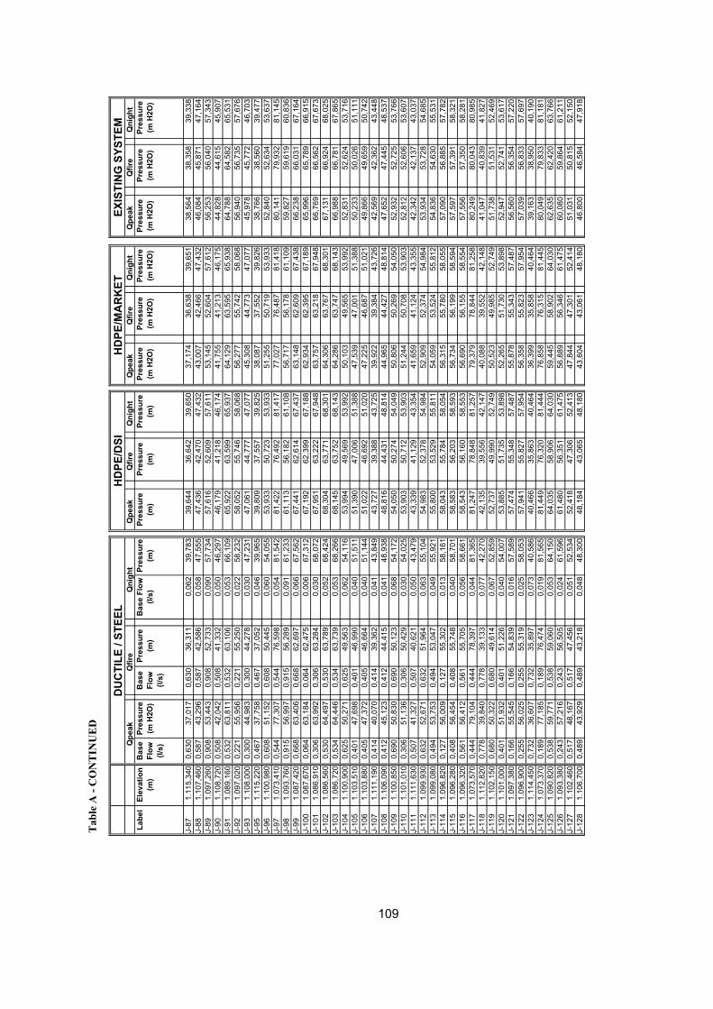
Tab
le A
- C
ON
TIN
UE
D
Qpe
ak
Qfir
e
Qni
ght
Qpe
ak
Qfir
e
Qni
ght
Qpe
ak
Qfir
e
Qni
ght
Labe
lEl
evat
ion
(m)
Bas
e Fl
ow
(l/s)
Pres
sure
(m
H2O
)B
ase
Flow
(l/
s)
Pres
sure
(m
)B
ase
Flow
(l/
s)Pr
essu
re
(m)
Pres
sure
(m
)Pr
essu
re
(m)
Pres
sure
(m
)Pr
essu
re
(m H
2O)
Pres
sure
(m
H2O
)Pr
essu
re
(m H
2O)
Pres
sure
(m
H2O
)Pr
essu
re
(m H
2O)
Pres
sure
(m
H2O
)
J-87
1.11
5,34
00,
630
37,0
170,
630
36,3
110,
062
39,7
8339
,644
36,6
4239
,650
37,1
7436
,638
39,6
5138
,564
38,3
5839
,338
J-88
1.10
7,46
00,
587
43,2
960,
587
42,5
860,
058
47,5
5547
,436
42,4
7047
,432
43,0
0742
,466
47,4
3246
,084
45,8
7147
,164
J-89
1.09
7,26
00,
908
53,4
430,
908
52,7
330,
090
57,7
3457
,616
52,6
0957
,611
53,1
4552
,604
57,6
1256
,253
56,0
4057
,343
J-90
1.10
8,72
00,
508
42,0
420,
508
41,3
320,
050
46,2
9746
,179
41,2
1846
,174
41,7
5541
,213
46,1
7544
,828
44,6
1545
,907
J-91
1.08
9,16
00,
532
63,8
110,
532
63,1
060,
053
66,1
0965
,922
63,5
9965
,937
64,1
2963
,595
65,9
3864
,788
64,5
8265
,531
J-92
1.09
7,02
00,
221
55,9
560,
221
55,2
500,
022
58,2
3258
,052
55,7
4658
,068
56,2
7755
,742
58,0
6856
,940
56,7
3557
,676
J-93
1.10
8,00
00,
300
44,9
830,
300
44,2
780,
030
47,2
3147
,061
44,7
7747
,077
45,3
0844
,773
47,0
7745
,978
45,7
7246
,703
J-95
1.11
5,22
00,
467
37,7
580,
467
37,0
520,
046
39,9
6539
,809
37,5
5739
,825
38,0
8737
,552
39,8
2638
,766
38,5
6039
,477
J-96
1.10
0,98
00,
608
51,1
520,
608
50,4
450,
060
54,0
5553
,933
50,7
2353
,933
51,2
5550
,719
53,9
3352
,840
52,6
3453
,637
J-97
1.07
3,41
00,
544
77,3
070,
544
76,5
980,
054
81,5
4281
,422
76,4
9281
,417
77,0
2776
,487
81,4
1880
,141
79,9
3281
,145
J-98
1.09
3,76
00,
915
56,9
970,
915
56,2
890,
091
61,2
3361
,113
56,1
8261
,108
56,7
1756
,178
61,1
0959
,827
59,6
1960
,836
J-99
1.08
7,42
00,
668
63,4
060,
668
62,6
970,
066
67,5
6267
,441
62,6
1467
,437
63,1
4862
,609
67,4
3866
,238
66,0
3167
,164
J-10
01.
087,
670
0,06
463
,184
0,06
462
,475
0,00
667
,312
67,1
9262
,399
67,1
8862
,934
62,3
9567
,189
65,9
9665
,789
66,9
15J-
101
1.08
6,91
00,
306
63,9
920,
306
63,2
840,
030
68,0
7267
,951
63,2
2267
,948
63,7
5763
,218
67,9
4866
,769
66,5
6267
,673
J-10
21.
086,
560
0,53
064
,497
0,53
063
,789
0,05
268
,424
68,3
0463
,771
68,3
0164
,306
63,7
6768
,301
67,1
3166
,924
68,0
25J-
103
1.08
6,72
00,
534
64,4
460,
534
63,7
390,
053
68,2
6668
,145
63,7
5268
,143
64,2
8663
,747
68,1
4366
,988
66,7
8167
,865
J-10
41.
100,
900
0,62
550
,271
0,62
549
,563
0,06
254
,116
53,9
9449
,569
53,9
9250
,103
49,5
6553
,992
52,8
3152
,624
53,7
16J-
105
1.10
3,51
00,
401
47,6
980,
401
46,9
900,
040
51,5
1151
,390
47,0
0651
,388
47,5
3947
,001
51,3
8850
,233
50,0
2651
,111
J-10
61.
103,
880
0,40
547
,372
0,40
546
,664
0,04
051
,144
51,0
2246
,692
51,0
2047
,225
46,6
8751
,021
49,8
6649
,659
50,7
42J-
107
1.11
1,19
00,
414
40,0
700,
414
39,3
620,
041
43,8
4943
,727
39,3
8843
,725
39,9
2239
,384
43,7
2642
,569
42,3
6243
,448
J-10
81.
106,
090
0,41
245
,123
0,41
244
,415
0,04
148
,938
48,8
1644
,431
48,8
1444
,965
44,4
2748
,814
47,6
5247
,445
48,5
37J-
109
1.10
0,85
00,
690
50,8
300,
690
50,1
230,
068
54,1
7254
,050
50,2
7454
,049
50,8
0650
,269
54,0
5052
,932
52,7
2553
,766
J-11
01.
101,
010
0,30
651
,136
0,30
650
,429
0,03
054
,025
53,9
0350
,712
53,9
0351
,244
50,7
0853
,903
52,8
1252
,606
53,6
07J-
111
1.11
1,63
00,
507
41,3
270,
507
40,6
210,
050
43,4
7943
,339
41,1
2943
,354
41,6
5941
,124
43,3
5542
,342
42,1
3743
,037
J-11
21.
099,
930
0,63
252
,671
0,63
251
,964
0,06
355
,104
54,9
8352
,378
54,9
8452
,909
52,3
7454
,984
53,9
3453
,728
54,6
85J-
113
1.09
9,08
00,
494
53,7
530,
494
53,0
470,
049
55,9
2155
,800
53,5
2955
,811
54,0
5953
,524
55,8
1254
,836
54,6
3055
,531
J-11
41.
096,
820
0,12
756
,009
0,12
755
,302
0,01
358
,161
58,0
4355
,784
58,0
5456
,315
55,7
8058
,055
57,0
9056
,885
57,7
82J-
115
1.09
6,28
00,
408
56,4
540,
408
55,7
480,
040
58,7
0158
,583
56,2
0358
,593
56,7
3456
,199
58,5
9457
,597
57,3
9158
,321
J-11
61.
096,
320
0,56
156
,412
0,56
155
,705
0,05
658
,661
58,5
4356
,160
58,5
5356
,690
56,1
5558
,554
57,5
5657
,350
58,2
81J-
117
1.07
3,57
00,
444
79,1
040,
444
78,3
970,
044
81,3
6581
,247
78,8
4881
,257
79,3
7978
,844
81,2
5880
,249
80,0
4380
,985
J-11
81.
112,
820
0,77
839
,840
0,77
839
,133
0,07
742
,270
42,1
3539
,556
42,1
4740
,088
39,5
5242
,148
41,0
4740
,839
41,8
27J-
119
1.10
2,15
00,
680
50,3
220,
680
49,6
140,
067
52,8
5952
,737
49,9
9052
,749
50,5
2349
,985
52,7
4951
,738
51,5
3152
,469
J-12
01.
101,
000
0,40
151
,932
0,40
151
,226
0,04
054
,007
53,8
8551
,735
53,8
9852
,265
51,7
3053
,898
52,9
4752
,741
53,6
17J-
121
1.09
7,38
00,
166
55,5
450,
166
54,8
390,
016
57,5
8957
,474
55,3
4857
,487
55,8
7855
,343
57,4
8756
,560
56,3
5457
,220
J-12
21.
096,
900
0,25
556
,025
0,25
555
,319
0,02
558
,053
57,9
4155
,827
57,9
5456
,358
55,8
2357
,954
57,0
3956
,833
57,6
97J-
123
1.11
4,45
00,
732
36,6
070,
732
35,8
970,
073
40,5
8640
,466
35,8
6340
,464
36,3
9935
,858
40,4
6439
,163
38,9
5040
,190
J-12
41.
073,
370
0,18
977
,185
0,18
976
,474
0,01
981
,565
81,4
4976
,320
81,4
4476
,858
76,3
1581
,445
80,0
4979
,833
81,1
81J-
125
1.09
0,82
00,
538
59,7
710,
538
59,0
600,
053
64,1
5064
,035
58,9
0664
,030
59,4
4558
,902
64,0
3062
,635
62,4
2063
,766
J-12
61.
093,
380
0,24
357
,216
0,24
356
,505
0,02
461
,596
61,4
8056
,351
61,4
7556
,889
56,3
4661
,475
60,0
8059
,864
61,2
11J-
127
1.10
2,46
00,
517
48,1
670,
517
47,4
560,
051
52,5
3452
,418
47,3
0652
,413
47,8
4447
,301
52,4
1451
,031
50,8
1552
,150
J-12
81.
106,
700
0,48
943
,929
0,48
943
,218
0,04
848
,300
48,1
8443
,065
48,1
8043
,604
43,0
6148
,180
46,8
0046
,584
47,9
18
Qpe
ak
Qfir
e
Qni
ght
DU
CTI
LE /
STEE
LH
DPE
/DSI
HD
PE/M
AR
KET
EXIS
TIN
G S
YSTE
M
109

Tab
le A
- C
ON
TIN
UE
D
Qpe
ak
Qfir
e
Qni
ght
Qpe
ak
Qfir
e
Qni
ght
Qpe
ak
Qfir
e
Qni
ght
Labe
lEl
evat
ion
(m)
Bas
e Fl
ow
(l/s)
Pres
sure
(m
H2O
)B
ase
Flow
(l/
s)
Pres
sure
(m
)B
ase
Flow
(l/
s)Pr
essu
re
(m)
Pres
sure
(m
)Pr
essu
re
(m)
Pres
sure
(m
)Pr
essu
re
(m H
2O)
Pres
sure
(m
H2O
)Pr
essu
re
(m H
2O)
Pres
sure
(m
H2O
)Pr
essu
re
(m H
2O)
Pres
sure
(m
H2O
)
J-12
91.
115,
620
0,37
235
,027
0,37
234
,316
0,03
739
,396
39,2
8134
,164
39,2
7734
,702
34,1
5939
,278
37,9
0237
,686
39,0
16J-
130
1.11
4,72
00,
343
35,9
630,
343
35,2
520,
034
40,2
9640
,181
35,1
1140
,177
35,6
4935
,106
40,1
7738
,805
38,5
8939
,914
J-13
11.
111,
170
0,42
839
,520
0,42
838
,810
0,04
243
,844
43,7
2838
,673
43,7
2339
,211
38,6
6843
,724
42,3
6242
,148
43,4
59J-
132
1.11
3,61
00,
166
37,0
790,
166
36,3
690,
016
41,4
0741
,291
36,2
3041
,287
36,7
6836
,225
41,2
8739
,917
39,7
0241
,023
J-13
31.
115,
470
0,28
235
,313
0,28
234
,601
0,02
839
,544
39,4
2934
,487
39,4
2735
,026
34,4
8239
,427
38,0
6037
,843
39,1
65J-
134
1.12
0,58
00,
535
30,2
160,
535
29,5
050,
053
34,4
4434
,329
29,3
9134
,327
29,9
3129
,387
34,3
2732
,960
32,7
4434
,066
J-13
51.
120,
180
0,30
830
,637
0,30
829
,926
0,03
134
,842
34,7
2729
,818
34,7
2630
,358
29,8
1434
,726
33,3
5933
,143
34,4
65J-
136
1.11
8,95
00,
446
31,7
270,
446
31,0
160,
044
36,0
6835
,952
30,8
6935
,951
31,4
0930
,865
35,9
5134
,583
34,3
6635
,692
J-13
71.
119,
360
0,60
231
,252
0,60
230
,541
0,06
035
,659
35,5
4330
,376
35,5
4130
,916
30,3
7235
,542
34,1
7033
,953
35,2
83J-
138
1.11
5,75
00,
605
34,8
560,
605
34,1
450,
060
39,2
6339
,147
33,9
8039
,144
34,5
2033
,976
39,1
4537
,772
37,5
5638
,886
J-13
91.
118,
850
0,65
431
,930
0,65
431
,219
0,06
536
,175
36,0
5931
,102
36,0
5631
,640
31,0
9736
,056
34,6
8934
,474
35,7
93J-
140
1.11
7,83
00,
549
32,7
780,
549
32,0
660,
054
37,1
8237
,066
31,9
0037
,065
32,4
4131
,896
37,0
6535
,699
35,4
8236
,809
J-14
11.
119,
170
0,63
131
,327
0,63
130
,615
0,06
335
,844
35,7
2830
,417
35,7
2630
,957
30,4
1235
,727
34,3
5434
,138
35,4
72J-
142
1.11
8,98
00,
305
31,5
150,
305
30,8
030,
030
36,0
3335
,918
30,6
0535
,916
31,1
4530
,600
35,9
1634
,544
34,3
2835
,662
J-14
31.
116,
090
0,89
334
,377
0,89
333
,665
0,08
938
,917
38,8
0133
,460
38,7
9934
,000
33,4
5638
,800
37,4
2837
,211
38,5
46J-
144
1.11
6,45
00,
612
34,0
010,
612
33,2
900,
061
38,5
5738
,442
33,0
8038
,440
33,6
2033
,076
38,4
4037
,068
36,8
5138
,187
J-14
51.
107,
260
1,25
443
,106
1,25
442
,394
0,12
447
,727
47,6
1142
,165
47,6
0942
,706
42,1
6147
,610
46,2
3346
,016
47,3
58J-
146
1.10
8,68
00,
894
41,6
900,
894
40,9
790,
089
46,3
0946
,194
40,7
5146
,192
41,2
9140
,746
46,1
9244
,817
44,5
9945
,940
J-14
71.
107,
610
0,22
742
,757
0,22
742
,045
0,02
247
,377
47,2
6241
,817
47,2
6042
,357
41,8
1247
,260
45,8
8445
,667
47,0
08J-
148
1.10
8,11
00,
437
42,2
800,
437
41,5
680,
043
46,8
7846
,763
41,3
4646
,761
41,8
8641
,341
46,7
6145
,397
45,1
7946
,509
J-14
91.
107,
650
0,48
542
,786
0,48
542
,074
0,04
847
,337
47,2
2241
,864
47,2
2042
,405
41,8
6047
,221
45,8
6445
,646
46,9
68J-
150
1.11
4,45
00,
144
35,9
990,
144
35,2
870,
014
40,5
5140
,436
35,0
7840
,434
35,6
1835
,073
40,4
3439
,077
38,8
5940
,182
J-15
11.
080,
520
0,18
269
,727
0,18
269
,015
0,01
874
,411
74,2
9668
,769
74,2
9469
,309
68,7
6474
,294
72,8
9172
,673
74,0
43J-
152
1.09
0,05
00,
613
60,2
170,
613
59,5
050,
061
64,9
0164
,785
59,2
5964
,783
59,8
0059
,254
64,7
8363
,381
63,1
6464
,532
J-15
31.
090,
060
0,62
360
,210
0,62
359
,498
0,06
264
,891
64,7
7559
,253
64,7
7359
,793
59,2
4864
,773
63,3
7363
,156
64,5
22J-
154
1.07
8,72
00,
481
71,5
250,
481
70,8
130,
048
76,2
0876
,093
70,5
6776
,090
71,1
0870
,562
76,0
9174
,690
74,4
7275
,839
J-15
51.
079,
490
0,35
770
,757
0,35
770
,045
0,03
575
,439
75,3
2469
,799
75,3
2270
,340
69,7
9475
,322
73,9
2373
,705
75,0
71J-
156
1.09
0,58
00,
364
59,6
910,
364
58,9
790,
036
64,3
7264
,257
58,7
3464
,254
59,2
7458
,729
64,2
5562
,857
62,6
3964
,003
J-15
71.
081,
490
0,41
568
,763
0,41
568
,051
0,04
173
,443
73,3
2867
,805
73,3
2668
,346
67,8
0173
,326
71,9
3371
,716
73,0
75J-
158
1.09
0,65
00,
753
59,6
240,
753
58,9
120,
075
64,3
0264
,187
58,6
6764
,184
59,2
0858
,663
64,1
8562
,791
62,5
7463
,933
J-15
91.
071,
850
0,37
178
,386
0,37
177
,674
0,03
783
,064
82,9
4977
,429
82,9
4677
,970
77,4
2582
,947
81,5
8381
,365
82,6
96J-
160
1.08
3,88
00,
606
66,3
920,
606
65,6
800,
060
71,0
5870
,943
65,4
3970
,941
65,9
7965
,434
70,9
4169
,579
69,3
6170
,690
J-16
11.
086,
410
0,58
863
,867
0,58
863
,155
0,05
868
,533
68,4
1862
,914
68,4
1663
,455
62,9
0968
,416
67,0
4766
,829
68,1
65J-
162
1.09
0,49
00,
919
59,8
630,
919
59,1
510,
091
64,4
6264
,347
58,9
2864
,345
59,4
6958
,923
64,3
4562
,995
62,7
7764
,094
J-16
31.
098,
160
0,33
752
,208
0,33
751
,496
0,03
356
,808
56,6
9251
,273
56,6
9051
,814
51,2
6956
,691
55,3
3255
,114
56,4
39J-
164
1.09
9,83
00,
701
50,5
410,
701
49,8
290,
069
55,1
4155
,026
49,6
0655
,024
50,1
4749
,601
55,0
2453
,663
53,4
4554
,772
J-16
51.
113,
510
0,65
837
,799
0,65
837
,086
0,06
541
,499
41,3
8337
,120
41,3
8437
,661
37,1
1541
,385
40,1
1039
,892
41,1
21J-
166
1.10
7,07
00,
444
44,2
370,
444
43,5
250,
044
47,9
2647
,810
43,5
6147
,811
44,1
0343
,556
47,8
1146
,545
46,3
2747
,549
J-16
71.
103,
830
0,44
047
,534
0,44
046
,821
0,04
451
,159
51,0
4346
,874
51,0
4447
,417
46,8
7051
,045
49,7
8949
,571
50,7
82J-
168
1.09
5,10
00,
609
56,2
780,
609
55,5
640,
060
59,8
6459
,750
55,6
2459
,752
56,1
6955
,619
59,7
5358
,528
58,3
0759
,493
J-16
91.
096,
400
0,45
456
,328
0,45
455
,600
0,04
558
,560
58,4
4556
,018
58,4
5456
,588
56,0
1358
,455
57,3
6957
,144
58,1
96J-
170
1.09
6,12
00,
090
56,7
430,
090
55,9
940,
009
58,8
2558
,711
56,4
2358
,724
57,0
2456
,417
58,7
2557
,716
57,4
5158
,469
J-17
11.
102,
340
0,39
249
,854
0,39
249
,145
0,03
952
,664
52,5
4349
,440
52,5
5349
,975
49,4
3552
,553
51,4
7651
,267
52,2
77J-
172
1.10
9,48
00,
630
41,1
890,
630
40,4
770,
062
45,5
1545
,399
40,3
3245
,398
40,8
7340
,328
45,3
9944
,055
43,8
3745
,142
J-17
31.
101,
790
0,46
648
,768
0,46
648
,056
0,04
653
,186
53,0
7147
,884
53,0
7048
,426
47,8
8053
,070
51,7
3351
,515
52,8
17
EXIS
TIN
G S
YSTE
MQ
peak
Q
fire
Q
nigh
t D
UC
TILE
/ ST
EEL
HD
PE/D
SIH
DPE
/MA
RK
ET
110

Tab
le A
- C
ON
TIN
UE
D
Qpe
ak
Qfir
e
Qni
ght
Qpe
ak
Qfir
e
Qni
ght
Qpe
ak
Qfir
e
Qni
ght
Labe
lEl
evat
ion
(m)
Bas
e Fl
ow
(l/s)
Pres
sure
(m
H2O
)B
ase
Flow
(l/
s)
Pres
sure
(m
)B
ase
Flow
(l/
s)Pr
essu
re
(m)
Pres
sure
(m
)Pr
essu
re
(m)
Pres
sure
(m
)Pr
essu
re
(m H
2O)
Pres
sure
(m
H2O
)Pr
essu
re
(m H
2O)
Pres
sure
(m
H2O
)Pr
essu
re
(m H
2O)
Pres
sure
(m
H2O
)
J-17
41.
098,
800
0,40
151
,754
0,40
151
,042
0,04
056
,170
56,0
5550
,871
56,0
5451
,412
50,8
6656
,054
54,7
2954
,511
55,8
01J-
175
1.09
7,23
00,
764
53,3
560,
764
52,6
430,
076
57,7
3757
,622
52,4
8257
,621
53,0
2352
,477
57,6
2156
,310
56,0
9157
,367
J-17
61.
057,
800
1,02
594
,717
1,02
593
,965
0,10
297
,064
96,9
5094
,310
96,9
6194
,920
94,3
0496
,962
95,9
1295
,640
96,7
10J-
177
1.09
2,83
01,
421
59,8
891,
421
59,1
360,
141
62,1
0661
,992
59,5
1962
,004
60,1
2959
,513
62,0
0560
,971
60,6
9961
,751
J-17
81.
065,
460
0,50
587
,125
0,50
586
,372
0,05
089
,420
89,3
0686
,733
89,3
1887
,342
86,7
2689
,318
88,2
0787
,934
89,0
65J-
179
1.08
3,15
00,
809
69,4
880,
809
68,7
350,
080
71,7
6671
,651
69,1
0071
,663
69,7
1069
,094
71,6
6470
,570
70,2
9771
,411
J-18
01.
095,
870
0,25
756
,986
0,25
756
,233
0,02
559
,074
58,9
5956
,653
58,9
7357
,263
56,6
4758
,973
57,9
5557
,683
58,7
17J-
181
1.09
5,42
01,
023
57,4
161,
023
56,6
460,
101
59,5
2059
,404
57,0
3659
,418
57,6
7557
,029
59,4
1858
,372
58,0
7359
,163
J-18
21.
091,
820
0,57
659
,908
0,57
659
,138
0,05
763
,097
62,9
8559
,218
62,9
9159
,858
59,2
1162
,992
60,8
6460
,566
62,7
41J-
183
1.07
9,68
00,
145
71,8
760,
145
71,1
060,
014
75,2
1175
,099
71,1
4575
,104
71,7
8471
,138
75,1
0572
,832
72,5
3474
,854
J-18
41.
091,
730
0,37
459
,851
0,37
459
,081
0,03
763
,185
63,0
7359
,120
63,0
7859
,759
59,1
1363
,079
60,8
0760
,509
62,8
29J-
185
1.08
4,05
00,
132
68,5
870,
132
67,6
310,
013
70,8
3270
,699
67,7
3770
,721
68,6
9767
,722
70,7
2269
,452
68,8
8070
,474
J-18
61.
094,
050
0,67
758
,607
0,67
757
,651
0,06
760
,852
60,7
2057
,758
60,7
4158
,717
57,7
4360
,742
59,4
7358
,901
60,4
95J-
187
1.06
3,99
00,
916
87,5
690,
916
86,9
880,
091
90,7
2390
,645
86,9
6790
,639
87,4
0586
,964
90,6
3989
,521
89,3
5090
,459
J-18
81.
084,
180
1,87
867
,514
1,87
866
,934
0,18
670
,575
70,4
9766
,939
70,4
9167
,377
66,9
3770
,492
69,4
6769
,296
70,3
11J-
189
1.10
0,05
00,
669
51,7
100,
669
51,1
290,
066
54,7
3754
,659
51,1
4454
,654
51,5
8251
,142
54,6
5453
,718
53,5
4754
,474
J-19
01.
105,
870
0,48
145
,923
0,48
145
,343
0,04
848
,929
48,8
5145
,364
48,8
4645
,802
45,3
6148
,846
47,9
1547
,744
48,6
66J-
191
1.11
5,12
00,
126
36,7
710,
126
36,1
910,
012
39,6
9939
,621
36,2
3439
,616
36,6
7236
,232
39,6
1638
,700
38,5
2839
,435
J-19
21.
120,
730
0,67
831
,231
0,67
830
,651
0,06
734
,101
34,0
2330
,710
34,0
1831
,149
30,7
0834
,019
33,1
1232
,941
33,8
36J-
193
1.11
2,84
00,
126
39,0
460,
126
38,4
660,
012
41,9
7441
,896
38,5
0941
,892
38,9
4738
,507
41,8
9240
,975
40,8
0341
,710
J-19
41.
102,
770
0,24
349
,015
0,24
348
,434
0,02
452
,023
51,9
4548
,455
51,9
4048
,893
48,4
5251
,940
51,0
0750
,835
51,7
60J-
195
1.11
3,31
00,
246
38,5
620,
246
37,9
810,
024
41,5
0541
,427
38,0
2041
,422
38,4
5838
,018
41,4
2240
,503
40,3
3241
,241
J-19
61.
099,
750
0,80
453
,201
0,80
452
,506
0,08
055
,195
55,0
8653
,007
55,0
9853
,530
53,0
0255
,099
54,2
0053
,997
54,8
47J-
197
1.12
3,47
01,
129
29,7
371,
129
29,1
470,
112
31,3
9331
,307
29,5
6931
,315
30,0
1629
,567
31,3
1530
,584
30,4
0531
,122
J-19
81.
126,
760
0,39
625
,681
0,39
625
,100
0,03
928
,090
28,0
1025
,291
28,0
0925
,730
25,2
8928
,009
27,1
5926
,988
27,8
20J-
199
1.12
4,87
00,
749
28,2
700,
749
27,6
900,
074
29,9
8629
,904
28,0
7929
,908
28,5
1828
,077
29,9
0829
,143
28,9
7229
,707
J-20
01.
105,
050
0,29
947
,658
0,29
946
,748
0,03
049
,806
49,6
9846
,833
49,7
1247
,755
46,8
2649
,712
48,4
9447
,940
49,4
97J-
201
1.10
4,96
00,
167
47,7
470,
167
46,8
360,
017
49,8
9649
,788
46,9
2049
,802
47,8
4246
,914
49,8
0248
,584
48,0
2949
,587
J-20
21.
105,
000
0,90
947
,705
0,90
946
,795
0,09
049
,856
49,7
4846
,879
49,7
6247
,800
46,8
7249
,762
48,5
4347
,988
49,5
47J-
203
1.09
3,44
00,
444
59,1
970,
444
58,2
210,
044
61,4
5761
,323
58,2
9661
,345
59,2
9158
,280
61,3
4660
,053
59,4
5161
,099
J-20
41.
124,
580
0,31
128
,598
0,31
128
,044
0,03
130
,234
30,1
5828
,409
30,1
6128
,830
28,4
0730
,161
29,4
5129
,286
29,9
85J-
205
1.12
4,58
00,
211
28,6
210,
211
28,0
790,
021
30,2
1830
,144
28,4
3430
,148
28,8
4728
,432
30,1
4829
,461
29,2
9829
,980
J-20
61.
124,
780
0,31
728
,462
0,31
727
,939
0,03
129
,998
29,9
2728
,280
29,9
3128
,680
28,2
7929
,931
29,2
7629
,118
29,7
74J-
207
1.12
5,73
00,
337
27,6
030,
337
27,1
140,
033
29,0
1828
,953
27,4
3328
,956
27,8
0827
,432
28,9
5628
,357
28,2
0528
,817
J-20
81.
124,
550
0,19
928
,867
0,19
928
,407
0,02
030
,174
30,1
1328
,711
30,1
1629
,065
28,7
1130
,115
29,5
6029
,414
29,9
87J-
209
1.12
3,05
00,
225
30,4
040,
225
29,9
550,
022
31,6
6231
,603
30,2
5431
,606
30,5
9930
,254
31,6
0631
,068
30,9
2431
,482
J-21
01.
119,
120
1,01
034
,464
1,01
034
,054
0,10
035
,560
35,5
0534
,339
35,5
0834
,655
34,3
4035
,508
35,0
2734
,890
35,3
96J-
211
1.12
3,46
01,
025
29,9
001,
025
29,3
800,
102
31,3
3531
,261
29,7
5031
,267
30,1
4629
,749
31,2
6730
,635
30,4
7331
,105
J-21
21.
117,
100
1,45
536
,492
1,45
536
,083
0,14
437
,576
37,5
2136
,370
37,5
2436
,684
36,3
7037
,524
37,0
4836
,913
37,4
12J-
213
1.11
4,90
01,
346
37,6
711,
346
36,6
400,
133
39,9
2039
,803
36,3
9639
,823
37,6
0336
,428
39,8
2138
,571
37,9
2439
,621
J-21
41.
116,
370
0,56
136
,327
0,56
135
,368
0,05
638
,410
38,3
0835
,143
38,3
2536
,273
35,1
8738
,321
37,1
9136
,603
38,1
45J-
215
1.11
4,55
00,
276
38,4
770,
276
37,7
240,
027
40,1
7540
,095
37,6
5340
,107
38,5
0437
,703
40,1
0239
,225
38,7
9739
,957
J-21
61.
089,
730
1,37
762
,656
1,37
761
,476
0,13
665
,058
64,9
2961
,089
64,9
5262
,522
61,1
1964
,951
63,5
6662
,786
64,7
40J-
217
1.09
0,59
02,
183
61,9
602,
183
60,8
930,
216
64,2
8964
,149
60,8
3664
,174
61,9
8760
,815
64,1
7662
,778
62,0
4263
,931
J-21
81.
089,
530
0,15
362
,851
0,15
361
,661
0,01
565
,264
65,1
3161
,272
65,1
5662
,716
61,2
9865
,155
63,7
4762
,941
64,9
41
HD
PE/D
SIH
DPE
/MA
RK
ETEX
ISTI
NG
SYS
TEM
Qpe
ak
Qfir
e
Qni
ght
DU
CTI
LE /
STEE
L
111

Tab
le A
- C
ON
TIN
UE
D
Qpe
ak
Qfir
e
Qni
ght
Qpe
ak
Qfir
e
Qni
ght
Qpe
ak
Qfir
e
Qni
ght
Labe
lEl
evat
ion
(m)
Bas
e Fl
ow
(l/s)
Pres
sure
(m
H2O
)B
ase
Flow
(l/
s)
Pres
sure
(m
)B
ase
Flow
(l/
s)Pr
essu
re
(m)
Pres
sure
(m
)Pr
essu
re
(m)
Pres
sure
(m
)Pr
essu
re
(m H
2O)
Pres
sure
(m
H2O
)Pr
essu
re
(m H
2O)
Pres
sure
(m
H2O
)Pr
essu
re
(m H
2O)
Pres
sure
(m
H2O
)
J-21
91.
089,
680
1,05
761
,696
1,05
760
,926
0,10
565
,228
65,1
1760
,908
65,1
2161
,548
60,9
0165
,121
62,6
5262
,354
64,8
72J-
220
1.07
5,92
01,
516
74,7
501,
516
73,9
800,
150
78,9
5178
,842
73,7
7178
,841
74,4
1173
,764
78,8
4275
,706
75,4
0878
,595
J-22
11.
076,
610
1,66
275
,613
1,66
274
,175
0,16
578
,194
78,0
3773
,632
78,0
6875
,401
73,5
8878
,071
76,3
0475
,027
77,8
35J-
222
1.09
0,22
00,
592
62,1
860,
592
61,0
390,
059
64,5
3164
,416
60,6
2864
,438
62,0
4960
,686
64,4
3263
,126
62,3
9364
,243
J-22
31.
078,
770
0,33
673
,577
0,33
672
,409
0,03
375
,954
75,8
4071
,911
75,8
6373
,415
72,0
1475
,855
74,5
2773
,764
75,6
68J-
224
1.08
1,57
00,
537
70,7
530,
537
69,5
610,
053
73,1
5673
,042
68,9
6573
,066
70,5
6769
,121
73,0
5771
,656
70,7
9072
,870
J-22
51.
071,
280
0,21
980
,782
0,21
979
,138
0,02
283
,498
83,3
3378
,327
83,3
6780
,445
78,2
6283
,371
81,3
7079
,741
83,1
34J-
226
1.07
1,31
01,
633
78,2
911,
633
72,9
810,
162
83,3
0583
,199
70,4
4683
,190
77,2
3670
,392
83,1
9181
,314
79,6
4683
,103
J-22
71.
071,
510
0,87
179
,058
0,87
178
,288
0,08
683
,351
83,2
4278
,053
83,2
4078
,692
78,0
4683
,241
80,0
1479
,716
82,9
95J-
228
1.06
9,74
00,
267
80,8
210,
267
80,0
510,
026
85,1
1885
,008
79,8
1585
,007
80,4
5579
,809
85,0
0781
,777
81,4
7984
,761
J-22
91.
101,
750
0,48
450
,835
0,48
449
,820
0,04
852
,976
52,8
8349
,403
52,9
0150
,721
49,5
3352
,891
51,7
1951
,045
52,7
30J-
230
1.08
1,59
00,
120
70,7
100,
120
69,4
960,
012
73,1
3773
,022
68,8
6073
,047
70,5
1269
,032
73,0
3771
,567
70,6
1872
,849
J-23
11.
081,
580
0,07
670
,720
0,07
669
,506
0,00
873
,147
73,0
3268
,870
73,0
5770
,522
69,0
4273
,047
71,5
7770
,628
72,8
59J-
232
1.07
4,61
00,
468
77,5
500,
468
76,2
070,
046
80,1
1379
,991
75,3
4480
,021
77,2
8775
,605
80,0
0878
,135
76,6
9979
,811
J-23
31.
068,
160
0,61
381
,400
0,61
376
,091
0,06
186
,449
86,3
4273
,546
86,3
3380
,336
73,4
9186
,334
84,4
2482
,756
86,2
46J-
234
1.07
8,69
00,
206
70,8
900,
206
65,5
810,
020
75,9
4075
,834
63,0
3575
,825
69,8
2562
,981
75,8
2573
,914
72,2
4675
,737
J-23
51.
088,
620
0,48
260
,176
0,48
253
,554
0,04
865
,972
65,8
7249
,973
65,8
5858
,869
50,3
4265
,864
63,5
2761
,001
65,7
97J-
236
1.08
7,70
00,
706
61,1
090,
706
54,4
880,
070
66,8
9166
,790
50,9
1166
,776
59,8
0651
,279
66,7
8264
,461
61,9
3566
,716
J-23
71.
078,
660
0,74
270
,126
0,74
263
,505
0,07
475
,912
75,8
1259
,928
75,7
9868
,822
60,2
9675
,804
73,4
7870
,955
75,7
37J-
238
1.08
1,42
00,
387
67,3
630,
387
60,7
430,
038
73,1
5873
,057
57,1
6373
,043
66,0
5757
,531
73,0
4970
,721
68,1
9872
,983
J-23
91.
074,
000
0,07
074
,786
0,07
068
,168
0,00
780
,563
80,4
6364
,594
80,4
4973
,485
64,9
6380
,454
78,1
3375
,612
80,3
88J-
240
1.07
8,84
00,
411
69,9
560,
411
63,3
380,
041
75,7
3375
,632
59,7
6475
,618
68,6
5560
,132
75,6
2473
,303
70,7
8275
,558
J-24
11.
091,
840
0,49
157
,013
0,49
150
,390
0,04
962
,759
62,6
5946
,822
62,6
4555
,721
47,1
9162
,651
60,3
6357
,829
62,5
84J-
242
1.08
4,05
00,
766
64,7
700,
766
58,1
540,
076
70,5
3470
,433
54,5
8570
,419
63,4
7354
,953
70,4
2568
,109
65,5
9070
,358
J-24
31.
099,
070
0,12
249
,938
0,12
243
,290
0,01
255
,545
55,4
4439
,749
55,4
3148
,684
40,1
2355
,437
53,1
5350
,618
55,3
69J-
244
1.10
5,61
00,
268
43,4
120,
268
36,7
500,
027
49,0
1748
,916
33,2
0848
,904
42,1
6033
,579
48,9
0946
,630
44,0
8448
,842
J-24
51.
106,
860
0,51
942
,168
0,51
935
,505
0,05
147
,769
47,6
6931
,964
47,6
5640
,916
32,3
3547
,662
45,3
8542
,840
47,5
94J-
246
1.10
1,65
00,
995
47,3
630,
995
40,7
080,
099
52,9
6952
,869
37,1
6652
,856
46,1
1037
,539
52,8
6250
,579
48,0
4052
,794
J-24
71.
097,
750
0,74
651
,203
0,74
644
,547
0,07
456
,861
56,7
6040
,990
56,7
4749
,935
41,3
6356
,753
54,4
1951
,879
56,6
85J-
248
1.11
6,17
00,
192
32,9
330,
192
26,2
330,
019
38,4
7638
,377
22,7
0538
,365
31,6
9623
,068
38,3
7036
,143
33,5
6138
,303
J-24
91.
130,
260
0,57
518
,872
0,57
512
,172
0,05
724
,414
24,3
168,
645
24,3
0317
,636
9,00
824
,308
22,0
8319
,500
24,2
41J-
250
1.12
9,48
00,
456
19,6
360,
456
12,9
420,
045
25,1
9325
,094
9,41
125
,081
18,3
959,
776
25,0
8722
,850
20,2
7325
,020
J-25
11.
126,
410
0,45
822
,687
0,45
815
,997
0,04
528
,257
28,1
5812
,460
28,1
4521
,443
12,8
2828
,151
25,9
0923
,334
28,0
83J-
252
1.12
4,43
00,
456
24,6
570,
456
17,9
690,
045
30,2
3330
,134
14,4
2930
,121
23,4
1214
,799
30,1
2727
,879
25,3
0630
,059
J-25
31.
112,
890
0,82
536
,168
0,82
529
,486
0,08
241
,749
41,6
5025
,947
41,6
3834
,920
26,3
1541
,643
39,3
9136
,824
41,5
76J-
254
1.11
2,47
00,
485
36,5
900,
485
29,9
070,
048
42,1
6942
,070
26,3
7142
,057
35,3
4326
,738
42,0
6239
,814
37,2
4841
,995
J-25
51.
112,
650
0,97
136
,421
0,97
129
,743
0,09
641
,988
41,8
9026
,224
41,8
7735
,177
26,5
7741
,882
39,6
4937
,113
41,8
15J-
256
1.12
4,17
00,
301
24,9
160,
301
18,2
280,
030
30,4
9330
,393
14,6
8930
,381
23,6
7015
,058
30,3
8628
,139
25,5
6530
,319
J-25
71.
113,
560
0,97
235
,487
0,97
228
,817
0,09
641
,082
40,9
8225
,277
40,9
7034
,236
25,6
4740
,975
38,7
0636
,153
40,9
08J-
258
1.11
2,81
00,
268
36,2
220,
268
29,5
540,
027
41,8
3141
,731
26,0
3141
,719
34,9
6726
,381
41,7
2439
,442
36,9
0141
,656
J-25
91.
108,
820
0,51
440
,201
0,51
433
,535
0,05
145
,814
45,7
1430
,018
45,7
0138
,946
30,3
6145
,706
43,4
2340
,884
45,6
38J-
260
1.09
9,68
00,
159
49,3
220,
159
42,6
560,
016
54,9
3554
,835
39,1
3954
,822
48,0
6739
,482
54,8
2852
,544
50,0
0554
,760
J-26
11.
110,
450
0,70
838
,576
0,70
831
,911
0,07
044
,190
44,0
8928
,465
44,0
7637
,322
28,7
3944
,081
41,7
9839
,282
44,0
13J-
262
1.09
6,15
00,
719
52,8
590,
719
46,2
630,
071
58,4
6258
,361
42,7
5758
,348
51,6
0843
,114
58,3
5356
,073
53,5
7058
,284
J-26
31.
098,
740
0,47
250
,268
0,47
243
,628
0,04
755
,875
55,7
7440
,091
55,7
6149
,015
40,4
6455
,767
53,4
8350
,952
55,6
98
EXIS
TIN
G S
YSTE
MQ
peak
Q
fire
Q
nigh
t D
UC
TILE
/ ST
EEL
HD
PE/D
SIH
DPE
/MA
RK
ET
112

Tab
le A
- C
ON
TIN
UE
D
Qpe
ak
Qfir
e
Qni
ght
Qpe
ak
Qfir
e
Qni
ght
Qpe
ak
Qfir
e
Qni
ght
Labe
lEl
evat
ion
(m)
Bas
e Fl
ow
(l/s)
Pres
sure
(m
H2O
)B
ase
Flow
(l/
s)
Pres
sure
(m
)B
ase
Flow
(l/
s)Pr
essu
re
(m)
Pres
sure
(m
)Pr
essu
re
(m)
Pres
sure
(m
)Pr
essu
re
(m H
2O)
Pres
sure
(m
H2O
)Pr
essu
re
(m H
2O)
Pres
sure
(m
H2O
)Pr
essu
re
(m H
2O)
Pres
sure
(m
H2O
)
J-26
41.
086,
580
0,79
162
,298
0,79
155
,716
0,07
868
,012
67,9
1052
,180
67,8
9761
,016
52,5
4067
,903
65,5
9563
,097
67,8
35J-
265
1.06
6,91
00,
197
81,9
240,
197
75,3
420,
020
87,6
4287
,541
71,8
0587
,527
80,6
4072
,164
87,5
3385
,224
82,7
2687
,465
J-26
61.
081,
040
0,29
667
,823
0,29
661
,241
0,02
973
,540
73,4
3957
,705
73,4
2666
,540
58,0
6473
,431
71,1
2368
,625
73,3
63J-
267
1.09
6,15
01,
066
52,8
681,
066
46,3
180,
106
58,4
6458
,362
42,8
3358
,350
51,6
2043
,185
58,3
5556
,079
53,6
0158
,285
J-26
81.
113,
280
1,15
835
,755
1,15
829
,078
0,11
541
,366
41,2
6725
,685
41,2
5434
,500
25,9
0241
,257
38,9
8436
,473
41,1
89J-
269
1.12
8,46
00,
540
20,7
000,
540
14,0
190,
053
26,2
1026
,112
10,5
3126
,099
19,4
7210
,870
26,1
0423
,903
21,3
3026
,038
J-27
01.
133,
790
0,80
915
,355
15,8
098,
292
0,08
020
,893
20,7
944,
765
20,7
8214
,119
4,99
120
,786
18,5
7815
,854
20,7
19J-
271
1.13
2,42
00,
505
16,7
0315
,505
9,49
90,
050
22,2
6022
,161
5,90
922
,148
15,4
636,
171
22,1
5319
,922
17,0
0822
,086
J-27
21.
124,
630
0,62
024
,463
0,62
017
,485
0,06
130
,034
29,9
3513
,974
29,9
2323
,219
14,2
2529
,927
27,6
8425
,029
29,8
60J-
273
1.12
1,14
00,
603
27,9
420,
603
21,1
420,
060
33,5
2133
,424
17,8
4433
,410
26,6
9617
,935
33,4
1331
,168
28,6
1533
,344
J-27
41.
130,
710
0,70
718
,405
0,70
711
,611
0,07
023
,971
23,8
758,
399
23,8
6117
,162
8,40
923
,863
21,6
4919
,112
23,7
94J-
275
1.12
3,19
00,
568
26,0
160,
568
19,4
970,
056
31,4
7131
,373
16,0
7031
,360
24,8
0316
,400
31,3
6529
,214
26,7
8731
,297
J-27
61.
121,
590
0,43
827
,657
0,43
821
,187
0,04
333
,065
32,9
6717
,940
32,9
5526
,455
18,1
2332
,960
30,8
3428
,432
32,8
94J-
277
1.11
6,02
00,
799
33,1
790,
799
26,7
600,
079
38,6
2238
,525
23,6
2838
,513
31,9
6723
,701
38,5
1836
,410
34,0
9838
,452
J-27
81.
118,
470
0,07
930
,835
0,07
924
,485
0,00
836
,177
36,0
8021
,448
36,0
6829
,650
21,4
7236
,073
34,0
1731
,741
36,0
07J-
279
1.11
8,98
00,
027
30,3
260,
027
23,9
760,
003
35,6
6835
,571
20,9
3935
,559
29,1
4120
,963
35,5
6433
,508
31,2
3335
,498
J-28
01.
118,
770
0,23
130
,535
0,23
124
,185
0,02
335
,878
35,7
8021
,148
35,7
6929
,350
21,1
7335
,774
33,7
1831
,442
35,7
07J-
281
1.11
9,13
00,
047
30,1
410,
047
23,7
990,
005
35,5
1835
,421
20,7
8335
,409
28,9
4620
,779
35,4
1433
,354
31,1
0135
,348
J-28
21.
117,
720
0,91
431
,609
0,91
425
,306
0,09
136
,925
36,8
2822
,353
36,8
1630
,431
22,3
1436
,822
34,7
9432
,568
36,7
55J-
283
1.11
7,77
00,
234
31,4
790,
234
25,1
370,
023
36,8
7536
,778
22,1
1536
,766
30,2
7922
,112
36,7
7134
,692
32,4
3936
,705
J-28
41.
119,
350
0,40
329
,909
0,40
323
,567
0,04
035
,298
35,2
0120
,548
35,1
8928
,711
20,5
4435
,195
33,1
2230
,869
35,1
28J-
285
1.11
8,88
00,
027
30,4
250,
027
24,0
760,
003
35,7
6835
,671
21,0
3835
,659
29,2
4021
,063
35,6
6433
,608
31,3
3235
,598
J-28
61.
117,
000
0,12
932
,240
0,12
925
,899
0,01
337
,643
37,5
4622
,875
37,5
3431
,038
22,8
7137
,540
35,4
5333
,201
37,4
73J-
287
1.11
8,30
00,
367
30,9
430,
367
24,6
020,
036
36,3
4636
,249
21,5
7836
,237
29,7
4121
,574
36,2
4234
,156
31,9
0436
,176
J-28
81.
111,
160
0,08
838
,069
0,08
831
,727
0,00
943
,472
43,3
7428
,703
43,3
6336
,867
28,7
0043
,368
41,2
8239
,029
43,3
02J-
289
1.13
6,56
00,
272
12,7
310,
272
6,38
90,
027
18,1
2318
,026
3,36
818
,014
11,5
323,
365
18,0
1915
,944
13,6
9117
,953
J-29
01.
120,
610
0,29
032
,033
0,29
030
,010
0,02
933
,945
33,9
0329
,197
33,8
9931
,725
29,1
8633
,901
31,9
5629
,786
33,8
70J-
291
1.12
5,02
00,
088
27,6
320,
088
25,6
090,
009
29,5
4429
,502
24,7
9629
,498
27,3
2424
,784
29,5
0027
,555
25,3
8529
,469
J-29
21.
121,
110
1,27
332
,994
1,27
332
,811
0,12
633
,407
33,3
8732
,929
33,3
8733
,071
32,9
2933
,387
33,2
1133
,149
33,3
51J-
294
1.12
5,31
00,
113
28,1
480,
113
27,7
370,
011
29,3
8129
,326
27,9
8429
,328
28,2
9927
,984
29,3
2828
,830
28,6
9329
,218
J-29
51.
133,
400
1,00
320
,075
1,00
319
,664
0,09
921
,307
21,2
5319
,911
21,2
5520
,226
19,9
1121
,254
20,7
5620
,620
21,1
45J-
296
1.14
2,08
00,
109
11,4
120,
109
11,0
010,
011
12,6
4512
,590
11,2
4812
,592
11,5
6311
,248
12,5
9212
,093
11,9
5712
,482
J-29
71.
095,
650
0,23
353
,371
0,23
346
,831
0,02
358
,964
58,8
6243
,353
58,8
4952
,124
43,7
0258
,855
56,5
8154
,109
58,7
84J-
298
1.09
0,15
00,
762
58,9
830,
762
52,8
790,
076
64,4
7064
,364
49,6
4164
,353
57,7
7649
,914
64,3
5862
,169
59,9
7864
,282
J-29
91.
082,
720
1,23
066
,455
1,23
060
,351
0,12
271
,886
71,7
8057
,128
71,7
6965
,264
57,4
0171
,774
69,6
0367
,412
71,6
97J-
300
1.08
3,92
00,
890
65,1
830,
890
58,9
110,
088
70,6
8170
,576
55,5
7270
,565
63,9
6955
,891
70,5
7168
,355
66,0
5770
,496
J-30
11.
087,
060
0,44
762
,019
0,44
755
,675
0,04
467
,545
67,4
4052
,297
67,4
2960
,796
52,6
2667
,434
65,2
0262
,857
67,3
61J-
302
1.10
1,96
00,
893
47,0
490,
893
40,4
370,
088
52,6
6552
,564
37,0
2552
,552
45,7
9437
,282
52,5
5650
,270
47,7
8052
,486
J-30
31.
090,
490
0,18
458
,495
0,18
451
,883
0,01
864
,112
64,0
1148
,471
63,9
9857
,240
48,7
2764
,003
61,7
1659
,225
63,9
33J-
304
1.09
9,51
00,
676
49,4
960,
676
42,8
390,
067
55,1
1055
,010
39,4
7354
,997
48,2
4139
,671
55,0
0152
,727
50,2
2554
,931
J-30
51.
094,
010
0,83
554
,986
0,83
548
,341
0,08
360
,599
60,5
0044
,976
60,4
8653
,731
45,1
7960
,490
58,2
1655
,715
60,4
20J-
306
1.08
6,88
00,
146
62,1
010,
146
55,4
560,
015
67,7
1567
,615
52,0
9167
,602
60,8
4652
,294
67,6
0665
,331
62,8
3167
,536
J-30
71.
083,
260
0,79
666
,062
0,79
660
,229
0,07
971
,358
71,2
5257
,232
71,2
4264
,916
57,4
0171
,245
69,1
6867
,155
71,1
65J-
308
1.08
6,45
00,
212
62,6
530,
212
56,3
730,
021
68,1
5768
,050
52,7
9268
,035
61,4
3253
,334
68,0
4665
,847
63,4
3567
,967
J-30
91.
096,
680
0,77
452
,445
0,77
446
,165
0,07
757
,948
57,8
4142
,585
57,8
2651
,225
43,1
2757
,837
55,6
3753
,226
57,7
58
HD
PE/D
SIH
DPE
/MA
RK
ETEX
ISTI
NG
SYS
TEM
Qpe
ak
Qfir
e
Qni
ght
DU
CTI
LE /
STEE
L
113

Tab
le A
- C
ON
TIN
UE
D
Qpe
ak
Qfir
e
Qni
ght
Qpe
ak
Qfir
e
Qni
ght
Qpe
ak
Qfir
e
Qni
ght
Labe
lEl
evat
ion
(m)
Bas
e Fl
ow
(l/s)
Pres
sure
(m
H2O
)B
ase
Flow
(l/
s)
Pres
sure
(m
)B
ase
Flow
(l/
s)Pr
essu
re
(m)
Pres
sure
(m
)Pr
essu
re
(m)
Pres
sure
(m
)Pr
essu
re
(m H
2O)
Pres
sure
(m
H2O
)Pr
essu
re
(m H
2O)
Pres
sure
(m
H2O
)Pr
essu
re
(m H
2O)
Pres
sure
(m
H2O
)
J-31
01.
118,
850
0,67
030
,213
0,67
023
,513
0,06
635
,808
35,7
1020
,186
35,6
9628
,963
20,3
3635
,699
33,4
4530
,928
35,6
30J-
311
1.11
7,36
00,
550
31,6
960,
550
25,0
000,
055
37,2
9537
,197
21,6
6537
,183
30,4
4521
,822
37,1
8734
,930
32,4
1337
,117
J-31
21.
104,
330
0,83
644
,687
0,83
638
,013
0,08
350
,299
50,2
0034
,660
50,1
8643
,432
34,8
3850
,190
47,9
1945
,414
50,1
21J-
313
1.12
0,86
00,
775
28,2
040,
775
21,4
640,
077
33,8
0133
,703
18,1
3433
,689
26,9
5318
,272
33,6
9331
,437
28,9
0833
,624
J-31
41.
127,
590
0,55
321
,498
0,55
314
,745
0,05
527
,085
26,9
8811
,471
26,9
7420
,250
11,5
5126
,976
24,7
3722
,210
26,9
08J-
315
1.12
7,38
00,
474
21,8
000,
474
15,2
940,
047
27,3
0027
,199
11,8
0227
,185
20,5
7712
,190
27,1
9124
,985
22,4
9927
,118
J-31
61.
120,
890
0,32
328
,338
0,32
322
,058
0,03
233
,785
33,6
7818
,358
33,6
6327
,133
19,0
3233
,675
31,4
7529
,036
33,5
95J-
317
1.12
2,19
00,
531
27,0
410,
531
20,7
610,
053
32,4
8832
,380
17,1
0132
,366
25,8
3617
,735
32,3
7730
,185
27,7
5732
,298
J-31
81.
123,
470
0,43
425
,735
0,43
419
,284
0,04
331
,202
31,1
0015
,783
31,0
8624
,522
16,2
0431
,093
28,9
1226
,482
31,0
19J-
319
1.12
8,55
00,
353
20,6
500,
353
14,1
790,
035
26,1
3326
,030
10,6
8026
,016
19,4
3211
,089
26,0
2323
,830
21,3
7925
,950
J-32
01.
107,
800
0,86
041
,503
0,86
035
,532
0,08
546
,862
46,7
5031
,939
46,7
3640
,326
32,6
1746
,749
44,5
8242
,270
46,6
63J-
321
1.11
7,68
00,
453
31,5
740,
453
25,4
240,
045
36,9
9436
,882
21,5
8936
,867
30,3
7822
,442
36,8
8334
,680
32,2
5136
,799
J-32
21.
091,
420
1,08
058
,185
1,08
052
,817
0,10
763
,233
63,1
2350
,144
63,1
1657
,099
50,1
4763
,118
61,1
4459
,282
63,0
25J-
323
1.10
7,72
00,
603
41,6
070,
603
35,6
720,
060
46,9
4346
,832
32,2
2046
,819
40,4
3732
,771
46,8
3044
,687
42,4
2946
,745
J-32
41.
105,
680
0,47
543
,570
0,47
537
,509
0,04
748
,974
48,8
5933
,607
48,8
4442
,380
34,5
5948
,862
46,6
5844
,248
48,7
76J-
325
1.07
4,29
00,
684
75,2
980,
684
69,9
610,
068
80,3
3080
,222
67,3
5380
,214
74,2
2867
,331
80,2
1578
,293
76,5
3980
,125
J-32
61.
093,
360
0,43
655
,982
0,43
650
,163
0,04
361
,279
61,1
6646
,696
61,1
5354
,828
47,3
1561
,166
59,0
4156
,848
61,0
78J-
327
1.10
2,47
00,
399
46,7
730,
399
40,7
120,
040
52,1
7852
,062
36,8
1452
,047
45,5
8337
,762
52,0
6549
,862
47,4
5251
,979
J-32
81.
079,
210
0,27
772
,949
0,27
771
,616
0,02
775
,513
75,3
9770
,755
75,4
2672
,686
71,0
1575
,411
73,5
4472
,114
75,2
21J-
329
1.08
3,60
00,
315
68,5
620,
315
67,2
380,
031
71,1
2371
,012
66,3
8071
,040
68,3
0066
,641
71,0
2369
,163
67,7
4170
,840
J-33
01.
089,
590
0,30
262
,583
0,30
261
,269
0,03
065
,135
65,0
3060
,415
65,0
5862
,322
60,6
8265
,038
63,1
8661
,776
64,8
62J-
331
1.09
5,68
00,
615
56,5
050,
615
55,2
060,
061
59,0
5058
,949
54,3
5258
,977
56,2
4554
,631
58,9
5657
,111
55,7
1158
,784
J-33
21.
079,
910
0,87
769
,679
0,87
764
,325
0,08
774
,721
74,6
1261
,680
74,6
0468
,600
61,6
7374
,606
72,6
5770
,848
74,5
14J-
333
1.11
1,98
00,
719
40,2
370,
719
38,9
400,
071
42,7
8142
,681
38,0
8742
,709
39,9
7738
,367
42,6
8740
,844
39,4
4742
,517
J-33
41.
110,
540
0,77
241
,690
0,77
240
,413
0,07
644
,217
44,1
1839
,590
44,1
4441
,437
39,8
5744
,124
42,3
1740
,979
43,9
54J-
335
1.10
4,44
00,
238
48,0
570,
238
46,9
860,
024
50,2
9450
,199
46,4
8150
,219
47,9
1046
,639
50,2
0748
,887
48,0
7650
,045
J-33
61.
108,
230
0,22
144
,168
0,22
143
,028
0,02
246
,514
46,4
1842
,413
46,4
4043
,981
42,6
0746
,426
44,9
2943
,946
46,2
61J-
337
1.10
8,86
00,
305
43,4
830,
305
42,3
020,
030
45,8
8745
,791
41,6
2445
,813
43,2
7541
,840
45,7
9844
,204
43,1
1845
,632
EXIS
TIN
G S
YSTE
MQ
peak
Q
fire
Q
nigh
t D
UC
TILE
/ ST
EEL
HD
PE/D
SIH
DPE
/MA
RK
ET
114