Water Hammer Analysis using a Hybrid Scheme. Análisis del

Water Hammer Analysis using a Hybrid Scheme.

Twyman. 16 - 25

Revista Científico Tecnológica Departamento Ingeniería de Obras Civiles RIOC Volumen 07/2017 ISSN 0719-0514 16

Water Hammer Analysis using a Hybrid Scheme. Análisis del Golpe de Ariete usando un Esquema Híbrido.

INFORMACIÓN DEL ARTÍCULO Article history: Received 17-07-2017 Accepted 18-08-2017 Available 17-10-2017 Keywords: Hybrid scheme Implicit finite − difference method (IFDM) Method of Characteristics (MOC) Pipe network Water hammer. Historial del artículo: Recibido 17-07-2017 Aceptado 18-08-2017 Publicado 17-10-2017 Palabras Clave: Golpe de ariete Método de diferencias finitas implícito (MDFI) Método de las Características (MC) Esquema híbrido Red de tuberías.

John Twyman Quilodrán1

1 Twyman Ingenieros Consultores, Rancagua, Chile.

[email protected], teléfono: 56-9-89044770

Abstract

Water hammer is analyzed using an original hybrid scheme that solves the transient flow by applying the Method of Characteristics (MOC) on those pipes with a Courant number equal or approximately equal to 1.0, and the Implicit Finite−Difference Method (IFDM) on the pipes with Courant less than 1.0. The proposed algorithm allows solve the transient flow problem applying the best method (MOC or IFDM) in each system pipe depending on the Courant number assigned to it. By analyzing the transient flow in two pipe networks it is demonstrated that this solution-type allows obtain almost exact and/or conservative solutions without consuming too many resources such as computational memory and software execution time.

Resumen

Se analiza el golpe de ariete utilizando un esquema híbrido original que resuelve el flujo transitorio aplicando el Método de las Características (MC) en aquellas tuberías con un número de Courant igual o aproximadamente igual a 1.0 y el Método de Diferencias Finitas Implícito (MDFI) en las tuberías con Courant inferior a 1.0. El algoritmo propuesto permite resolver el problema del flujo transitorio aplicando el mejor método (MC o MDFI) en cada tubería del sistema, dependiendo del número de Courant que tenga asignado. Al analizar el flujo transiente en dos redes de tuberías se demuestra que este tipo de solución permite obtener soluciones casi exactas y/o conservadoras sin consumir demasiados recursos relacionados con la memoria computacional y el tiempo de ejecución del software.


Twyman. 16 - 25


1. Introduction.

In the modern era the transient flow study has occupied the attention of prominent researchers since the late eighteenth century, when Euler made his first contributions on the subject [25]. This process had a renewed impetus in the mid-1960s when Streeter and Lai [18] presented the first studies using computational methods. This was the beginning of a need tide related to the efficient pipe networks modelling, with the objective of assuring design and operation levels that would allow

reduce the costs and ensure the longevity of the systems with a minimum of service interruption. Despite the theoretical development observed internationally in the last decades, the quantity of computer programs and specialized services for the water hammer analysis is not abundant. This may be because of the problem complexity where the research and development (R&D) can take several years. In general, knowledge about the subject can be mainly sought on universities and some international engineering and consulting companies (Table 1).

Table 1: Some institutions and companies dedicated to the water hammer study and solution.

Institution Software name Solution method

Applied Flow Technology AFT Impulse Method of Characteristics (MOC)

Flow Science Inc. FLOW 3−D TruVOF

Hydromantis Inc. ARTS MOC

BHR Group FLOWMASTER 2 MOC

Bentley Systems, Inc. HAMMER MOC

Stoner Associates, Inc. LIQT MOC

DHI HYPRESS Finite-Difference Method (4th order)

University of Auckland HYTRAN MOC

University of Cambridge PIPENET Transient Module MOC

University of Kentucky SURGE Wave Method (WM)

University of Toronto TRANSAM MOC

Univ. Politécnica de Valencia DYAGATS MOC

Univ. Politécnica de Valencia ARhIETE MOC

WL / Delft Hydraulics WANDA MOC

US Army Corps Engineers WHAMO Implicit Finite-Difference Method

(IFDM)

DHI MIKE URBAN MOC

Innovyze H2O SURGE WM

KYPIPE SURGE WM

EPA EPA SURGE WM

Unisont Engineering, Inc. uSLAM MOC


Twyman. 16 - 25


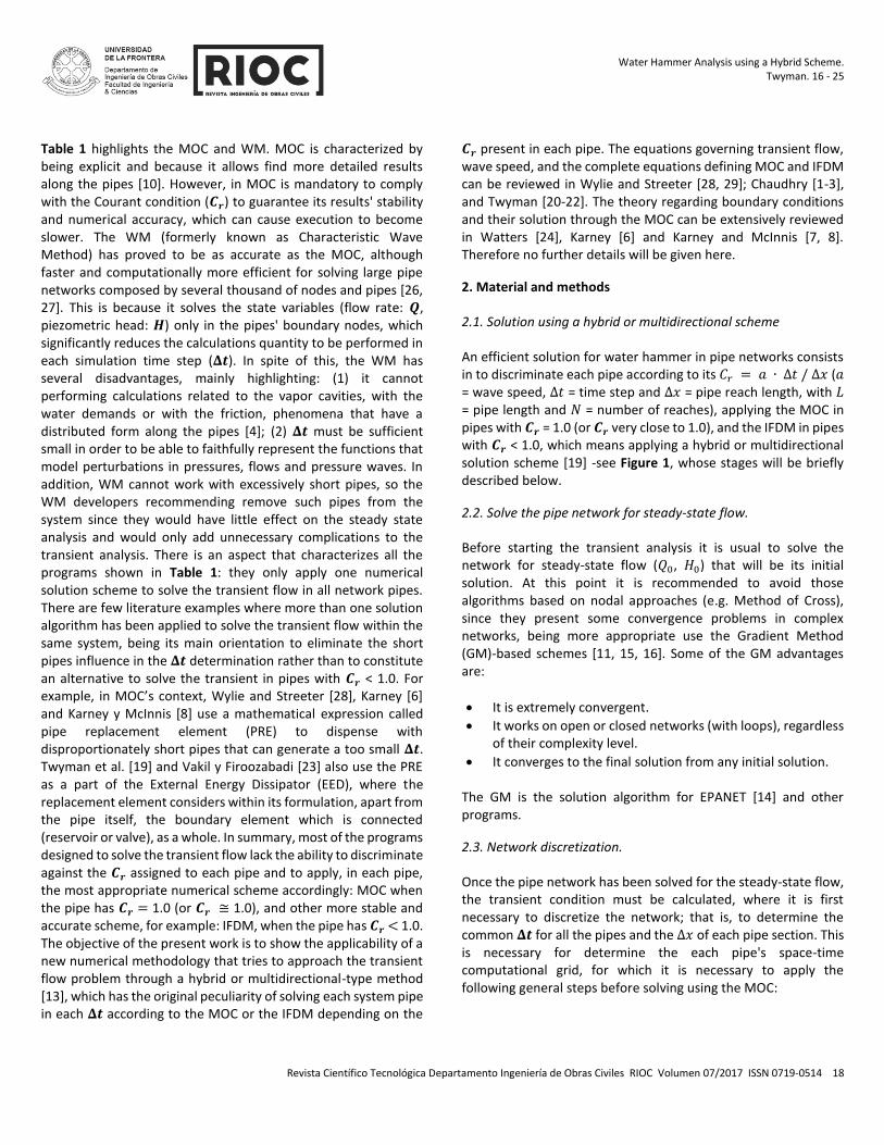
Table 1 highlights the MOC and WM. MOC is characterized by being explicit and because it allows find more detailed results along the pipes [10]. However, in MOC is mandatory to comply with the Courant condition (𝑪𝒓) to guarantee its results' stability and numerical accuracy, which can cause execution to become slower. The WM (formerly known as Characteristic Wave Method) has proved to be as accurate as the MOC, although faster and computationally more efficient for solving large pipe networks composed by several thousand of nodes and pipes [26, 27]. This is because it solves the state variables (flow rate: 𝑸, piezometric head: 𝑯) only in the pipes' boundary nodes, which significantly reduces the calculations quantity to be performed in each simulation time step (𝚫𝒕). In spite of this, the WM has several disadvantages, mainly highlighting: (1) it cannot performing calculations related to the vapor cavities, with the water demands or with the friction, phenomena that have a distributed form along the pipes [4]; (2) 𝚫𝒕 must be sufficient small in order to be able to faithfully represent the functions that model perturbations in pressures, flows and pressure waves. In addition, WM cannot work with excessively short pipes, so the WM developers recommending remove such pipes from the system since they would have little effect on the steady state analysis and would only add unnecessary complications to the transient analysis. There is an aspect that characterizes all the programs shown in Table 1: they only apply one numerical solution scheme to solve the transient flow in all network pipes. There are few literature examples where more than one solution algorithm has been applied to solve the transient flow within the same system, being its main orientation to eliminate the short pipes influence in the 𝚫𝒕 determination rather than to constitute an alternative to solve the transient in pipes with 𝑪𝒓 < 1.0. For example, in MOC’s context, Wylie and Streeter [28], Karney [6] and Karney y McInnis [8] use a mathematical expression called pipe replacement element (PRE) to dispense with disproportionately short pipes that can generate a too small 𝚫𝒕. Twyman et al. [19] and Vakil y Firoozabadi [23] also use the PRE as a part of the External Energy Dissipator (EED), where the replacement element considers within its formulation, apart from the pipe itself, the boundary element which is connected (reservoir or valve), as a whole. In summary, most of the programs designed to solve the transient flow lack the ability to discriminate against the 𝑪𝒓 assigned to each pipe and to apply, in each pipe, the most appropriate numerical scheme accordingly: MOC when the pipe has 𝑪𝒓 = 1.0 (or 𝑪𝒓 ≅ 1.0), and other more stable and accurate scheme, for example: IFDM, when the pipe has 𝑪𝒓 < 1.0. The objective of the present work is to show the applicability of a new numerical methodology that tries to approach the transient flow problem through a hybrid or multidirectional-type method [13], which has the original peculiarity of solving each system pipe in each 𝚫𝒕 according to the MOC or the IFDM depending on the

𝑪𝒓 present in each pipe. The equations governing transient flow, wave speed, and the complete equations defining MOC and IFDM can be reviewed in Wylie and Streeter [28, 29]; Chaudhry [1-3], and Twyman [20-22]. The theory regarding boundary conditions and their solution through the MOC can be extensively reviewed in Watters [24], Karney [6] and Karney and McInnis [7, 8]. Therefore no further details will be given here.

2. Material and methods

2.1. Solution using a hybrid or multidirectional scheme

An efficient solution for water hammer in pipe networks consists in to discriminate each pipe according to its 𝐶𝑟 = 𝑎 ∙ Δ𝑡 / Δ𝑥 (𝑎 = wave speed, Δ𝑡 = time step and Δ𝑥 = pipe reach length, with 𝐿 = pipe length and 𝑁 = number of reaches), applying the MOC in pipes with 𝑪𝒓 = 1.0 (or 𝑪𝒓 very close to 1.0), and the IFDM in pipes with 𝑪𝒓 < 1.0, which means applying a hybrid or multidirectional solution scheme [19] -see Figure 1, whose stages will be briefly described below.

2.2. Solve the pipe network for steady-state flow.

Before starting the transient analysis it is usual to solve the network for steady-state flow (𝑄0, 𝐻0) that will be its initial solution. At this point it is recommended to avoid those algorithms based on nodal approaches (e.g. Method of Cross), since they present some convergence problems in complex networks, being more appropriate use the Gradient Method (GM)-based schemes [11, 15, 16]. Some of the GM advantages are:

It is extremely convergent.

It works on open or closed networks (with loops), regardless of their complexity level.

It converges to the final solution from any initial solution. The GM is the solution algorithm for EPANET [14] and other programs.

2.3. Network discretization.

Once the pipe network has been solved for the steady-state flow, the transient condition must be calculated, where it is first necessary to discretize the network; that is, to determine the common 𝚫𝒕 for all the pipes and the Δ𝑥 of each pipe section. This is necessary for determine the each pipe's space-time computational grid, for which it is necessary to apply the following general steps before solving using the MOC:


Twyman. 16 - 25


Figure 1: basic hybrid or multidirectional scheme flowchart (tf = maximum simulation time).

Choose the system's shortest pipe (control pipe). Assign a value to 𝑁0, for example, 1, 2 or 3 (𝑁0 = number of reaches of the shortest pipe).

Calculate ∆𝑥0 = 𝐿0/𝑁0 (𝐿0 = length of the shortest pipe).

Calculate the wave speed 𝑎0 for the shortest pipe.

Once 𝑎0 is calculated, suppose that shortest pipe fulfill with Courant, that is: 𝐶𝑛 = 𝑎0 ∙ (∆𝑡/∆𝑥0) = 1.0.

Calculate ∆𝑡 = 𝐿0/(𝑁0 ∙ 𝑎0), which corresponds to the simulation time step.

Known Δ𝑡 suppose for the rest of pipes that 𝐶𝑛 = 𝑁 ∙ 𝑎 ∙(∆𝑡/𝐿) = 1.0.

With each pipe data, calculate 𝑁 = 𝑖𝑛𝑡[𝐿/(𝑎 ∙ ∆𝑡)], where the term 𝑖𝑛𝑡 means positive integer value.

Once known 𝑁, calculate ∆𝑥 = 𝐿/𝑁. The procedure shown above allows calculate the simulation time step (∆𝑡), the shortest pipe's reach (∆𝑥0) and the reach (∆𝑥) for the remaining network´s pipes. With this it is possible to define

the space - time grid needed to apply the MOC in each pipe.

2.4. Calculate 𝐻 and 𝑄 for every network node using the MOC.

It is possible to apply a useful approach to model different boundary conditions (or hydraulic devices), which facilitates 𝑄 and 𝐻 calculation [6, 8, 17, 19]:

𝐻𝑃𝑡+∆𝑡 = 𝐶𝑐 − 𝐵𝑐 ∙ 𝑄𝑒𝑥𝑡 (1)

Where 𝐻𝑃𝑡+∆𝑡 = pressure at the pipes point junction; 𝐶𝑐 and 𝐵𝑐 =

known constants and 𝑄𝑒𝑥𝑡 = external nodal flow, which may be constant, a function of time or some constitutive relation (polytropic equation). The compatibility equation (1) allows easily solve the transient flow in complex networks composed of simple nodes, reservoirs, valves, etc., where it is enough to know the 𝑄𝑒𝑥𝑡 analytical expression for each of these boundary conditions

in order to determine 𝐻𝑃𝑡+∆𝑡 value at each simulation time step.

2.5. For each pipe: verify 𝐶𝑟 value.

This action is verified with 𝐶𝑟 values calculated in step 2.3.

Solve the pipe network for steady-

state flow

t < tf

t = t + ∆t

Stop

Cr = 1 (or Cr ≈ 1)

Calculate H and Qfor every boundary

node using the MOC

For every pipe: verify the Cr value

Calculate H and Qfor every internal

node

Discretize the pipe network Build the system A ‧ y = b

using the IFDM, tridiagonalize and solve using the Thomas

algorithm

1

1

YES

NO

NO

YES

Apply MOC


Twyman. 16 - 25


2.6. If 𝐶𝑟 < 1.0. Build system 𝐴 ∙ 𝑦 = 𝑏 using the IFDM and then solve it.

The system of equations is constructed from the dynamics and continuity equations that define the transient flow, and it can be expressed for each discretized pipe as follows in IFDM's terms:

𝑑1𝑄𝑖𝑡+∆𝑡 + 𝑑2𝑄𝑖+1

𝑡+∆𝑡 − 𝑑3𝐻𝑖𝑡+∆𝑡 + 𝑑3𝐻𝑖+1

𝑡+∆𝑡 + 𝑑4 = 0 (2)

−𝑐1𝑄𝑖𝑡+∆𝑡 + 𝑐1𝑄𝑖+1

𝑡+∆𝑡 + 𝑐2𝐻𝑖𝑡+∆𝑡 + 𝑐3𝐻𝑖+1

𝑡+∆𝑡 + 𝑐4 = 0 (3)

In the system 𝐴 ∙ 𝑦 = 𝑏, 𝑦 is a vector which includes the variables

𝑄𝑖𝑡+∆𝑡 and 𝐻𝑖

𝑡+∆𝑡, with 𝑖 = 1, 2, …, 𝑁 + 1, 𝑏 is a vector which includes the coefficients 𝑐4 and 𝑑4 for each internal node and for the pipe’s boundary conditions (upstream and downstream), and 𝐴 is a matrix which includes the coefficients 𝑑1, 𝑑2, 𝑑3, 𝑐1, 𝑐2 and 𝑐3. By means of a suitable arrangement, the matrix 𝐴 can be converted in a three-banded matrix which can be solved quickly and efficiently using Thomas algorithm, also known as double-sweep algorithm [12].

2.7., 2.8. Calculate 𝐻 and 𝑄 for each internal node.

For the pipe which will be solved by MOC, the following system of equations must be solved for each internal node (or section):

𝐻𝑃𝑡+∆𝑡 = 𝐶𝑃 −

𝑎

𝑔𝐴𝑃

𝑄𝑃𝑡+∆𝑡 (4)

𝐻𝑃𝑡+∆𝑡 = 𝐶𝑀 +

𝑎

𝑔𝐴𝑃

𝑄𝑃𝑡+∆𝑡 (5)

Where 𝐶𝑃 and 𝐶𝑀 are known constants, 𝑔 = acceleration due to gravity and 𝐴𝑃 = pipe cross-section. For the pipes solved by the IFDM the solution for each section is known from the solution of the system 𝐴 ∙ 𝑦 = 𝑏, as is shown in step 2.6. The hybrid scheme is exempt from performing interpolations in the pipe sections when 𝐶𝑟 < 1.0 because it solves each pipe using the MDFI, all of which leads to results with fewer errors (attenuations) in comparison with the traditional MOC.

3. Results: example 1.

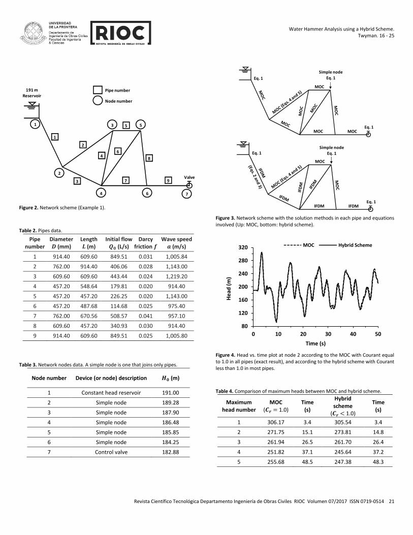
The method described above will be applied to solve water hammer in the pipe network shown in Figure 2, which also includes numbering of pipes and nodes. The system has nine pipes, seven nodes, three loops, one constant level reservoir (𝐻0 = 191 m) and a fast closure valve (𝑇𝑐 = 0.8 s) located at the downstream end of pipe 9. All the network nodes have elevation

0 (m). Tables 2 and 3 show the system's data (pipes and nodes). The maximum simulation time is 50 (s). The steady-state flow was solved using EPANET software [14]. Note: for clarity, the term pipe is henceforth restricted to conduits that contain at least one characteristic reach. The end of each reach, where head and flow values must be determined, is called a section. At sections internal to a pipe, the discharge can be obtained from (4) or (5). However, at each end of the pipe an auxiliary relation between head and discharge must be specified. Such a head-discharge relation is called a boundary condition. The term node indicates a location where boundary sections meet [8]. In all cases of the example 1 nodes will be solved using the MOC (equation 1), and each pipe section will be solved by applying:

MOC (exact solution), which means that all pipes have 𝐶𝑟 = 1.0. This is achieved by adopting ∆𝑡 = 0.1 (s) and 𝑁 = 6, 8, 5, 6, 4, 5, 7, 5 and 6 for pipes 1 to 9, respectively.

Hybrid scheme in some pipes with 𝐶𝑟 < 1.0. This requires discretizing the network as follows: ∆𝑡 = 0.08 (s) and 𝑁 = 6, 10, 4, 5, 5, 4, 6, 6 and 5 for pipes 1 to 9, respectively, being 𝐶𝑟 equal to: 0.79, 1.00, 0.64, 0.67, 1.00, 0.64, 0.69, 0.96 and 0.66.

Figure 3 shows the network scheme together with the main equations involved in the transient flow calculation when applying the MOC or the hybrid scheme. Figure 4 shows the result obtained when the transient flow is solved by MOC with 𝐶𝑟 = 1.0 in all pipes, and when the hybrid scheme is applied with 𝐶𝑟 < 1.0 in most pipes. The hybrid scheme solves sections in pipes 1, 3, 4, 6, 7 and 9 using the IFDM. In the remaining pipes (2, 5 and 8) sections are solved via the MOC. Both the result for MOC and the hybrid scheme are shown in separate curves in order to visualize the curves shape in both cases. Observing the results of Figure 4, it is noticed at first sight that the hybrid scheme shows for node 2 a pressure vs. time curve very similar to that given by the MOC (exact). Tables 4 and 5 summarize the maximum and minimum pressures (Figure 4) obtained by the MOC (exact, 𝐶𝑟 = 1.0) and by the hybrid scheme (𝐶𝑟 < 1.0) at different simulation times.


Twyman. 16 - 25


Figure 2. Network scheme (Example 1).

Table 2. Pipes data.

Pipe number

Diameter 𝑫 (mm)

Length 𝑳 (m)

Initial flow 𝑸𝟎 (L/s)

Darcy friction 𝒇

Wave speed 𝒂 (m/s)

1 914.40 609.60 849.51 0.031 1,005.84

2 762.00 914.40 406.06 0.028 1,143.00

3 609.60 609.60 443.44 0.024 1,219.20

4 457.20 548.64 179.81 0.020 914.40

5 457.20 457.20 226.25 0.020 1,143.00

6 457.20 487.68 114.68 0.025 975.40

7 762.00 670.56 508.57 0.041 957.10

8 609.60 457.20 340.93 0.030 914.40

9 914.40 609.60 849.51 0.025 1,005.80

Table 3. Network nodes data. A simple node is one that joins only pipes.

Node number Device (or node) description 𝑯𝟎 (m)

1 Constant head reservoir 191.00

2 Simple node 189.28





7 Control valve 182.88

Figure 3. Network scheme with the solution methods in each pipe and equations involved (Up: MOC, bottom: hybrid scheme).

Figure 4. Head vs. time plot at node 2 according to the MOC with Courant equal to 1.0 in all pipes (exact result), and according to the hybrid scheme with Courant less than 1.0 in most pipes.

Table 4. Comparison of maximum heads between MOC and hybrid scheme.

Maximum head number

MOC (𝑪𝒓 = 1.0)

Time (s)

Hybrid scheme

(𝑪𝒓 < 1.0)

Time (s)

1 306.17 3.4 305.54 3.4

2 271.75 15.1 273.81 14.8

3 261.94 26.5 261.70 26.4

4 251.82 37.1 245.64 37.2

5 255.68 48.5 247.38 48.3

Valve

191 mReservoir

Pipe number

2

Node number

1

2

3

5

4

7 9

8

4

3

6

5

6

1

7

Eq. 1

Simple nodeEq. 1

Eq. 1

MOC

MOCMOC

Eq. 1Simple node

Eq. 1

Eq. 1

MOC

IFDMIFDM

80

120

160

200

240

280

320

0 10 20 30 40 50

He

ad (

m)

Time (s)

MOC Hybrid Scheme


Twyman. 16 - 25


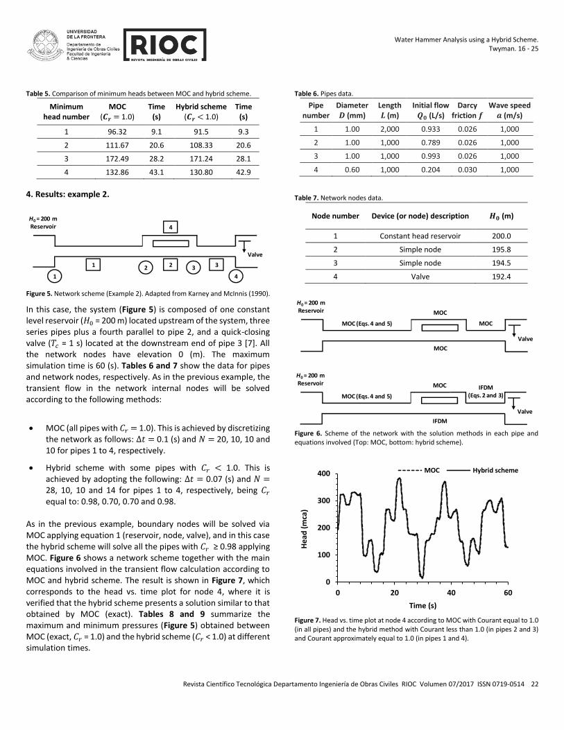
Table 5. Comparison of minimum heads between MOC and hybrid scheme.

Minimum head number

MOC (𝑪𝒓 = 1.0)

Time (s)

Hybrid scheme (𝑪𝒓 < 1.0)

Time (s)

1 96.32 9.1 91.5 9.3

2 111.67 20.6 108.33 20.6

3 172.49 28.2 171.24 28.1

4 132.86 43.1 130.80 42.9

4. Results: example 2.

Figure 5. Network scheme (Example 2). Adapted from Karney and McInnis (1990).

In this case, the system (Figure 5) is composed of one constant level reservoir (𝐻0 = 200 m) located upstream of the system, three series pipes plus a fourth parallel to pipe 2, and a quick-closing valve (𝑇𝑐 = 1 s) located at the downstream end of pipe 3 [7]. All the network nodes have elevation 0 (m). The maximum simulation time is 60 (s). Tables 6 and 7 show the data for pipes and network nodes, respectively. As in the previous example, the transient flow in the network internal nodes will be solved according to the following methods:

MOC (all pipes with 𝐶𝑟 = 1.0). This is achieved by discretizing the network as follows: ∆𝑡 = 0.1 (s) and 𝑁 = 20, 10, 10 and 10 for pipes 1 to 4, respectively.

Hybrid scheme with some pipes with 𝐶𝑟 < 1.0. This is achieved by adopting the following: ∆𝑡 = 0.07 (s) and 𝑁 = 28, 10, 10 and 14 for pipes 1 to 4, respectively, being 𝐶𝑟 equal to: 0.98, 0.70, 0.70 and 0.98.

As in the previous example, boundary nodes will be solved via MOC applying equation 1 (reservoir, node, valve), and in this case the hybrid scheme will solve all the pipes with 𝐶𝑟 ≥ 0.98 applying MOC. Figure 6 shows a network scheme together with the main equations involved in the transient flow calculation according to MOC and hybrid scheme. The result is shown in Figure 7, which corresponds to the head vs. time plot for node 4, where it is verified that the hybrid scheme presents a solution similar to that obtained by MOC (exact). Tables 8 and 9 summarize the maximum and minimum pressures (Figure 5) obtained between MOC (exact, 𝐶𝑟 = 1.0) and the hybrid scheme (𝐶𝑟 < 1.0) at different simulation times.

Table 6. Pipes data.

Pipe number

Diameter 𝑫 (mm)

Length 𝑳 (m)

Initial flow 𝑸𝟎 (L/s)

Darcy friction 𝒇

Wave speed 𝒂 (m/s)

1 1.00 2,000 0.933 0.026 1,000

2 1.00 1,000 0.789 0.026 1,000

3 1.00 1,000 0.993 0.026 1,000

4 0.60 1,000 0.204 0.030 1,000

Table 7. Network nodes data.

Node number Device (or node) description 𝑯𝟎 (m)

1 Constant head reservoir 200.0

2 Simple node 195.8

3 Simple node 194.5

4 Valve 192.4

Figure 6. Scheme of the network with the solution methods in each pipe and equations involved (Top: MOC, bottom: hybrid scheme).

Figure 7. Head vs. time plot at node 4 according to MOC with Courant equal to 1.0 (in all pipes) and the hybrid method with Courant less than 1.0 (in pipes 2 and 3) and Courant approximately equal to 1.0 (in pipes 1 and 4).

H0 = 200 mReservoir

Valve

1

2 3

4

1 2 3

4

H0 = 200 mReservoir

Valve

MOC (Eqs. 4 and 5)

MOC

MOC

MOC

H0 = 200 mReservoir

Valve

MOC (Eqs. 4 and 5)

MOC

IFDM

IFDM (Eqs. 2 and 3)

0

100

200

300

400

0 20 40 60

He

ad (

mca

)

Time (s)

MOC Hybrid scheme


Twyman. 16 - 25


Tables 8 and 9 show a comparison between the maximum and minimum pressures obtained between MOC (exact, 𝐶𝑟 = 1.0) and the hybrid scheme (𝐶𝑟 < 1.0) at different simulation times.

Table 8. Comparison of maximum heads between MOC and hybrid scheme.

Maximum head number

MOC (𝑪𝒓 = 1.0)

Time (s)

Hybrid scheme

(𝑪𝒓 < 1.0)

Time (s)

1 330.98 6.0 331.56 5.8

2 380.97 21.9 383.64 21.8

3 365.57 37.9 370.92 37.8

4 300.14 53.8 302.66 53.8

Table 9. Comparison of minimum heads between MOC and hybrid scheme.

Minimum head number

MOC (𝑪𝒓 = 1.0)

Time (s)

Hybrid scheme (𝑪𝒓 < 1.0)

Time (s)

1 37.38 13.9 35.69 13.8

2 18.11 29.9 13.55 29.8

3 63.74 45.9 59.06 45.8

5. Discussion.

When analyzing the maximum pressures of Example 1 (Table 4), it is verified that the maximum error between the hybrid scheme and the MOC is less than +4%. In the case of the minimum pressures (Table 5), this error is less than +5%. In comparison to MOC, the application of the hybrid scheme means a little significant computational resources expenditure. For example, in the case analyzed (example 1), the MOC discretized the network with 𝑁𝑡𝑜𝑡𝑎𝑙 = 52, with the program execution time being 2.4 (s). In contrast, the hybrid scheme required 𝑁𝑡𝑜𝑡𝑎𝑙 = 51, with a system of equations of maximum size equal to 22x22 corresponding to the pipe 2. In addition, it took only 7.9 (s) to solve the problem considering a maximum simulation time of 50 (s). In case of having applied the IFDM as unique solution algorithm, the size of the system of equations would have been at least equal to 112x112, with a significant and expected increase in the use of computational resources. In analyzing the maximum pressures of Example 2 (Table 8), it is observed that the error between the hybrid scheme and the MOC is less than +2%. In the case of the minimum pressures (Table 9), the hybrid scheme is more conservative, with differences varying between -5% and -25% in the minimum pressure numbers 2 and 3, respectively. The application of the hybrid scheme also does not represent a significant computational resources expense, in this case MOC needed to discretize the network with 𝑁𝑡𝑜𝑡𝑎𝑙 = 50, with a program execution time equal to 2.6 (s).

In contrast, the hybrid scheme required 𝑁𝑡𝑜𝑡𝑎𝑙 = 62, being the maximum size of the system of equations to be solved, at each time step, equal to 58x58, corresponding to pipe 1. In addition, it took only 8.7 (s) to solve the problem. In case of having applied the IFDM as a unique solution algorithm, the size of the system of equations would have been at least equal to 128x128, with an expected increase in the use of computational resources. Examples 1 and 2 were carried out on a standard PC @ 1.66 (GHz). The option of applying the IFDM or the MOC in the pipe sections depending on whether the 𝐶𝑟 of the pipe is lower or greater than a control value CV (for example, 0.98, as adopted in example 2), allows a more efficient modeling, because it is meaningless in numerical terms to apply the IFDM in a section with a 𝐶𝑟 very close to 1.0, e.g. 𝐶𝑟 = 0.98, where MOC aplication is more practical without compromising the accuracy level neither the solution stability in significant way. Another interesting aspect of hybrid scheme is that it can change its nature depending on the value that CV takes. For example, when CV = 0 (zero), then the hybrid scheme solves all pipes using MOC. This option is useful to apply when the network has only pipes with 𝐶𝑟 = 1.0. When CV varies between 0 and 1, not including extreme values, the hybrid scheme described in this article applies. When CV = 1, then the IFDM is applied as the only solution scheme. This solution is valid when all pipes have 𝐶𝑟 < 1.0 (this case is more theoretical than practical because the pre-specified time interval discretization scheme always assigns 𝐶𝑟 = 1.0 to the system shortest pipe). In both analyzed examples the hybrid scheme meets the condition proposed by Kepler [9] and Wylie [30], who indicating that only when 𝜓∗ = ∆𝑡 ∙ 𝑓 ∙ 𝑉0/2𝐷 ≤ 0.02 is possible to ensure that any method delivers accurate results. Evaluating the equation 𝜓∗ in the examples 1 and 2 is verified for hybrid scheme, and its value

oscillates between 1.3 ‧ 10−3 and 2.4 ‧ 10−3. In the example 2, the

range for 𝜓∗ oscillates between 9.1 ‧ 10−4 and 1.3 ‧ 10−3. A hybrid

scheme disadvantage is that it must work with a 𝑁 = 3 as a minimum in those pipes where the IFDM is applied, because the pipe discretization must have two pipe reaches at least (one upstream and the other downstream) in order to apply the equations corresponding to boundary nodes, plus an additional pipe reach where to apply the IFDM's dynamics and continuity equations. However, this imposition is offset by the fact that the IFDM, unlike MOC, requires a smaller increase in the total 𝑁 amount in order to comply with 𝐶𝑟 in all system pipes, which could strongly influence the ∆𝑡 magnitude. Another IFDM's disadvantage is that it can report some numerical instability (spurious oscillations) when it is applied in pipes with 𝐶𝑟 < 0.5, situation that can be easily corrected by slightly increasing 𝑁 size (or what is the same, decreasing the ∆𝑥 size) in affected pipes.


Twyman. 16 - 25


6. Conclusions.

It is a fact that pipe networks are generally composed of pipes with various physical characteristics, and it is also a fact that some water hammer solution schemes, such as the MOC, before their execution, must resort to certain shortcuts, such as alteration of pipe lengths (𝐿) or wave speed (𝑎) adjustment in order to redraw the network discretization and thus to be able to fulfill the Courant condition, thus assuring the results' stability and numerical accuracy. These shortcuts, despite their wide acceptance (and application) in the water hammer theoretical and practical areas, have the disadvantage that they can alter the initial conditions together with the physics of the problem [5], with the risk of leading to results that can be physically incompatible, fictitious or without practical application [21]. Another way is to keep unchanged 𝑎 and/or 𝐿 values, and fine-tune both the discretization and the pipe reach length Δ𝑥 = 𝐿 / 𝑁, which may increase 𝑁 size. Nevertheless, it is clear that the application of these measures becomes obsolete when the design engineer seeks to solve the problem without altering any initial condition, and most importantly, without significantly increasing total 𝑁 size. Both conditions constitute a new demand level for available waterhammer programs, especially those MOC-based. In this sense, the hybrid scheme is a good alternative solution since it avoids applying a single solution algorithm in networks where there are many pipes with 𝐶𝑟 < 1.0, maintaining good numerical performance (processing speed, accuracy and numerical stability) without the need for modify any initial system parameter. The hybrid scheme shown in this article, based on a network decoupling, opens the way to implement other solution methods different than IFDM for the pipe sections with 𝐶𝑟 < 1.0, such as McCormack Method, which is 100% explicit and more stable than MOC.

7. References

[1] Chaudhry M.H. (1979). Applied Hydraulic Transients, p. 266, New York: Van Nostrand Reinhold. *p. 27-73, 302-331

[2] Chaudhry M.H. (1982). Numerical Solution of Transient−Flow Equations. Proc. Speciality Conf. Hydraulics Division, ASCE, Jackson, MS, 633−656.

[3] Chaudhry M.H. (2014). Applied Hydraulic Transients, p. 583, New York: Springer−Verlag.

[4] Ebacher G., Besner M.−C., Lavoie J., Jung B.S., Karney B.W., Prévost M. (2011). Transient Modeling of a Full−Scale Distribution System: Comparison with Field Data. Journal of Water Resources Planning and Management, 137(2): 173−182. DOI: 10.1061/(ASCE)WR.1943-5452.0000109

[5] Ghidaoui M.S., Karney B.W. (1994). Equivalent Differential Equations in Fixed−Grid Characteristics Method. Journal of Hydraulic Engineering, 120(10): 1159−1175.

[6] Karney B.W. (1984). Analysis of Fluids Transients in Large Distribution Networks. PhD Thesis. Vancouver: University of British Columbia. http://hdl.handle.net/2429/25312

[7] Karney B.W., McInnis D. (1990). Transient Analysis of Water Distribution Systems. Journal of AWWA, 62−70.

[8] Karney B.W., McInnis D. (1992). Efficient Calculation of Transient Flow in Simple Pipe Networks. Journal of Hydraulic Engineering, 118(7): 1014−1030.

[9] Kepler, A.K. (2007). Leak Detection and Calibration of Transient Hydraulic System Models. Thesis (Doctoral). São Carlos: University of São Paulo.

[10] Nascimento T.A. (2015). Análisis de los Métodos de Cálculo del Golpe de Ariete en las Tuberías. Trabajo de Graduación en Ingeniería Mecánica. Guaratinguetá: Universidad Estatal Paulista.

[11] Pilati S., Todini E. (1984). La Verifica delle Reti Idrauliche in Pressione. Instituto di Costruzione Idraulica, Facolta D’ Ingegneria dell Universita di Bologna.

[12] Press W.H., Flannery B.P., Teukolsky S.A., Vetterling W.T. (1986). Numerical Recipes, the Art of Scientific Computing, p. 933, New York: Cambridge University Press. *p. 43

[13] Radulj D. (2010). Assessing the Hydraulic Transient Performance of Water and Wastewater Systems using Field and Numerical Modeling Data. Toronto: U. of Toronto.

[14] Rossman L.A. (2000). EPANET 2 User’s Manual, p. 200, Cincinnati: US Environmental Protection Agency (EPA).

[15] Salgado R.O., Todini E., O’Connell P.E. (1987, 8-10 September). Comparison of the Gradient Method with some Traditional Methods for the Analysis of Water Supply Distribution Networks. Proceedings of the International Conference on Computer Applications for Water Supply and Distribution, Leicester Polytechnic (UK).

[16] Salgado R.O. (1988). Computer Modelling of Water Supply Networks Using the Gradient Method. Ph.D. Thesis. Newcastle upon Tyne: University of Newcastle upon Tyne.

[17] Salgado R., Zenteno J., Twyman C., Twyman J. (1993, 7-9 September). A Hybrid Characteristics−Finite Difference Method for Unsteady flow in Pipe Networks, International Conference on Integrated Computer Applications for Water Supply and Distribution (139-150). Leicester.

http://hdl.handle.net/2429/25312


Twyman. 16 - 25


[18] Streeter V.L., Lai C. (1963). Waterhammer Analysis Including Fluid Friction. Trans. Am. Soc. Civ. Eng., 128: 1491−1524.

[19] Twyman J., Twyman C., Salgado R.O. (1997, 22-24 octubre). Optimización del Método de las Características para el Análisis del Golpe de Ariete en Redes de Tuberías. XIII Congreso Chileno de Ingeniería Hidráulica (53-62). Santiago de Chile: SOCHID.

[20] Twyman J. (2016a, 26-30 Septiembre). Golpe de Ariete en una Red de Distribución de Agua. Anales del XXVII Congreso Latinoamericano de Hidráulica (pp. 10). Lima: IAHR (Spain Water and IWHR China).

[21] Twyman J. (2016b). Wave Speed Calculation for Water Hammer Analysis. Obras y Proyectos, 20: 86−92. ISSN: 0718−2813. http://dx.doi.org/10.4067/S0718-28132016000200007

[22] Twyman J. (2017). Water Hammer Analysis in a Water Distribution System. Ingeniería del Agua, 21(2): 87−102. https://doi.org/10.4995/Ia.2017.6389

[23] Vakil A., Firoozabadi B. (2006). Effect of Unsteady Friction Models and Friction−Loss Integration on Transient Pipe Flow, Scientia Iranica, Sharif University of Technology, 13(3): 245−254.

[24] Watters G.Z. (1984). Analysis and Control of Unsteady Flow in Pipelines, p. 349, Boston: Butterworth−Heinemann.

[25] Wood F.M. (1970). History of Water−Hammer. CE Research Report No. 65, Queen’s University at Kingston, Ontario, Canada.

[26] Wood D.J. 2005. Water Hammer Analysis−Essential and Easy (And Efficient). Journal of Environmental Engineering, ASCE, 131(8): 1123−1131.

[27] Wood D.J., Lingireddy S., Boulos P.F., Karney B.W., McPherson D.L. (2005). Numerical Methods for Modeling Transient Flow in Distribution Systems. Journal of AWWA, 97(7): 104−115.

[28] Wylie E.B., Streeter V.L. (1978). Fluid Transients, p. 206. McGraw−Hill International Book Company. *p. 17-65, 86-101, 180-189.

[29] Wylie E.B., Streeter V.L. (1993). Fluid Transients in Systems, p. 463. Pearson.

[30] Wylie E.B. (1996, 16-18 April). Unsteady Internal Flows − Dimensionless Numbers & Time Constants. Proceedings of the VII International Conference on Pressure Surges and Fluid Transients in Pipelines and Open Channels (283-288). Harrogate: Pressure Surges Publications.

Documents

Water Hammer Analysis using a Hybrid Scheme. Análisis del