Water-Level scheduling for parallel tasks in compute

Noname manuscript No.(will be inserted by the editor)

Water-Level scheduling for parallel tasks incompute-intensive application components

Robert Dietze · Michael Hofmann ·Gudula Rünger

Received: date / Accepted: date

Abstract The development of complex simulations with high computationaldemands often requires an efficient parallel execution of a large number of nu-merical simulation tasks. Exploiting heterogeneous compute resources for theexecution of parallel tasks can be achieved by integrating dedicated schedul-ing methods into the complex simulation code. In this article, the efforts fordeveloping an application from the area of engineering optimization consist-ing of various individual components are described. Several scheduling meth-ods for distributing parallel simulation tasks among heterogeneous computenodes are presented. Performance results and comparisons are shown for twonovel scheduling methods and several existing scheduling algorithms for paral-lel tasks. A heterogeneous compute cluster is used to demonstrate the schedul-ing and execution of benchmark tasks and FEM simulation tasks.

Keywords component-based development · distributed simulations · paralleltasks · scheduling methods · heterogeneous platforms

1 Introduction

Complex simulations in science and engineering often comprise of large num-bers of compute-intensive numerical tasks that dominate significantly the time-to-solution. Increasing the problem sizes for these kinds of applications is usu-ally limited since the number of tasks and their individual execution timesshould not be too high. Exploiting HPC resources, such as current heteroge-neous platforms or future ultrascale computing systems [6], provides an im-portant way to overcome such limitations. However, especially for a variablenumber of tasks that can be executed in parallel itself (i. e., parallel tasks), the

Robert Dietze · Michael Hofmann · Gudula RüngerDepartment of Computer Science, Technische Universität Chemnitz, Chemnitz, GermanyE-mail: {dirob,mhofma,ruenger}@cs.tu-chemnitz.de

Original published: R. Dietze, M. Hofmann, and G. Rünger. Water-Level scheduling for parallel tasks in compute-intensiveapplication components. The Journal of Supercomputing, Special Issue on Sustainability on Ultrascale Computing Systems andApplications, 72(11):4047–4068, 2016. Online available at http://dx.doi.org/10.1007/s11227-016-1711-1.

http://dx.doi.org/10.1007/s11227-016-1711-1

2 R. Dietze et al.

efficient utilization of compute resources requires dedicated scheduling meth-ods to be integrated and used within the application program.

The complex simulation which we consider is an application from mechani-cal engineering for optimizing lightweight structures based on numerical simu-lations. This class of applications is extensively studied in the research projectMERGE1 in a research group comprising of mathematicians, computer scien-tists, and especially mechanical engineers who are interested in developing newlightweight parts and constructions. The simulations cover the manufacturingprocess of short fiber-reinforced plastics and the characterization of their me-chanical properties for specific operating load cases [9]. To optimize these partsand constructions, an optimization problem is set up which is then solved byperforming the simulations several times with different parameter sets. Thegoal is to develop an optimal set of parameters. The optimization problemis to be solved using HPC platforms with a variety of compute nodes anddepending on the specific optimization problem at hand it is desirable to beable to port the optimization software to very different platforms. This leadsto some challenges for the parallel and distributed implementation.

The aim of the software development is twofold. On the one hand, thespecific optimization problem developed in the project should be implementedsuch that the software is able to run on very different hardware and for ap-plications of different sizes. Thus, the software should be sustainable in thesense that it can be easily adapted by the mechanical engineer or mathemati-cian. On the other hand, different simulation and optimization problems mightcome up and the software development process itself should be sustainable sothat new applications can be easily implemented. Our approach is to builda flexible application program whose individual components can be easily re-placed or extended. Long-term reusability of the application program (e. g., forincreasing problem scales) is achieved by a thorough support for distributedand heterogeneous platforms. Executing the simulations efficiently on a va-riety of HPC platforms leads to a scheduling problem for parallel tasks onheterogeneous compute nodes.

In this article, we present a component-based approach for the developmentof a complex simulation application from engineering optimization. Especially,we investigate the use of scheduling methods for assigning simulation tasks tocompute resources with the goal to reduce the total parallel runtime of the en-tire simulations. We employ task and data parallel scheduling and propose twonew scheduling methods for parallel tasks. The Water-Level method usesa best-case estimation of the total parallel runtime to determine the computeresources for each parallel task. The Water-Level-Search method repeatsthe Water-Level method several times to achieve an iterative improvementof the resulting schedule. All presented methods have been implemented andwe show performance results with different tasks on a heterogeneous computecluster.

1 MERGE Technologies for Multifunctional Lightweight Structures, http://www.tu-chemnitz.de/merge

http://www.tu-chemnitz.de/merge

http://www.tu-chemnitz.de/merge

Water-Level scheduling for parallel tasks 3

The three benchmarks for testing the scheduling methods developed havebeen chosen carefully to reflect different potential behavior of the parallel exe-cution time of parallel tasks in a set of tasks to be scheduled. The benchmarkfor synthetic parallel tasks is described by a runtime formula of the parallelexecution time in which the parallelization overhead can be modified througha parameter, thus reflecting very different performance behavior. A benchmarkfrom numerical linear algebra consists of a set of matrix multiplication taskseach of which executes a DGEMM operation from the OpenBLAS library [16]using matrices of size 4000 × 4000. This benchmark leads to parallel taskswhich have the same execution time and scale well up to the full number ofcores of a single compute node. The last benchmark comes from the complexapplication code that we consider, in which a set of simulation tasks has to beexecuted. The specific simulation tasks needed in the application code lead toparallel tasks that scale moderately well and, hence, the goal is to achieve aperformance improvement by our scheduling methods.

The rest of the article is organized as follows: Section 2 describes the appli-cation from mechanical engineering. Section 3 presents the component-basedapplication development. Section 4 presents the scheduling methods for exe-cuting the simulations on heterogeneous compute resources. Section 5 showscorresponding performance results. Section 6 discusses related work and Sect. 7concludes the article.

2 Simulation and Optimization of Lightweight Structures

The numerical optimization of lightweight structures consisting of fiber-re-inforced plastics to be developed in the project MERGE is performed by asimulation approach described in the following.

2.1 Simulation of fiber-reinforced plastics

The lightweight structures are manufactured by injection molding, which rep-resents one of the most economically important processes for the mass produc-tion of plastic parts. The parts are produced by injecting molten plastic into amold, followed by a cooling process. Fillers, such as glass or carbon fibers, aremixed into the plastic to improve mechanical properties, such as the stiffnessor the durability of the parts. Besides the properties of the materials used,the orientation of the fibers and the residual stresses within the parts havea strong influence on the resulting mechanical properties. Thus, determiningthe mechanical properties of such short fiber-reinforced plastics requires toconsider both the manufacturing process and specific operating load cases forthe potential use of the plastic parts.

The manufacturing process is simulated with a computational fluid dynam-ics (CFD) method that simulates the injection of the material until the moldis filled. The input data of the CFD simulation include the geometry of the

4 R. Dietze et al.

Optimization problem Optimized parameters

Selection of parameter configurations

Execution of simulation tasks

Evaluation of simulation results

Figure 1 Overview of the coarse structure of the optimization process for lightweight struc-tures.

part, the material properties, such as the viscosity or the percentage of mixedin fibers, and the manufacturing parameters, such as the injection position orpressure. The results of the simulation describe the fiber orientation and thetemperature distribution within the part. These results are used for simulat-ing the subsequent cooling process with a finite element method (FEM) thatcomputes the residual stresses within the frozen part.

The simulation of the manufacturing process is followed by an evaluationof the resulting part. Mechanical properties are determined by simulating thebehavior of the manufactured part for specific operating load cases of its fu-ture use. These simulations are also performed by FEM simulations. Boundaryconditions represent the given load cases. The FEM application code employsadvanced material laws for short fiber-reinforced plastics and uses the pre-viously determined fiber orientation and residual stresses within the part asinput data. The final simulation results describe the behavior of the part, forexample, its deformation under an applied surface load.

2.2 Optimization of manufacturing parameters

The goal of the simulation process is not only to simulate one specific manufac-turing process of a plastic part but to optimize the properties of the lightweightstructures. This is achieved by an optimization process that varies materialand manufacturing parameters, such as the fiber percentage or the injectionposition. Figure 1 shows a coarse overview of the optimization process. Theoptimization is executed by repeatedly selecting specific values for the param-eters to be used and then simulating the manufacturing process and the loadcases with the selected parameter configurations as described in the previoussubsection. Thus, there is a number of simulation tasks to be executed (i. e.,one for each parameter configuration to be simulated) that are independentfrom each other. The specific number of independent simulation tasks dependsstrongly on the number of parameters to be varied and on the optimizationmethod to be employed.

Solving optimization problems with objective functions that involve numer-ical simulations leads to various challenges, such as high computational costsfor each evaluation of the objective function, missing derivatives of the objec-


tive function, discontinuous and noisy simulation results in many cases, andlarge numbers of evaluations required for high-dimensional parameter spaces.Therefore in engineering optimization, techniques based on metamodels (orsurrogate models) are often used [24]. The goal of these techniques is to createan alternative model of the function that maps input parameters of experi-ments to experimental results. A small number of experiments, e. g. compu-tationally expensive simulations, is used for the training of a metamodel thatis inexpensive to evaluate. The metamodel can then be used for the predic-tion of experimental results for various input parameters which have not beensimulated, for example, to solve an optimization problem.

The optimization of lightweight structures is performed with a Krigingmetamodel approach for the global optimization [12] that proceeds as follows.Initial input parameter configurations for creating a metamodel are chosenbased on statistical methods for the design of experiments (i. e., either fullfactorial or Latin Hypercube) [14]. The objective function is evaluated foreach initial configuration and the results are used to train the metamodel.The Kriging metamodel provides an interpolation-based method that is espe-cially appropriate for deterministic computer experiments [25]. Furthermore,the Kriging metamodel allows the calculation of the expected improvementfor new parameter configurations, thus providing an efficient method for de-termining new candidates for parameter configurations of the optimizationprocess. The objective function is evaluated for each candidate and the re-sults are used to refine the metamodel. After a specific number of refinementsteps, the best remaining candidate is chosen as the optimal solution of theoptimization problem.

Evaluating the objective function involves the execution of the simulationtasks and is the most time consuming part of the optimization process. How-ever, since the evaluations are independent from each other, the simulationtasks can be executed at the same time. Thus, the chosen optimization methodprovides the opportunity to parallelize the evaluations during both the initialtraining step and in each refinement step. The actual number of evaluationsdepends, for example, on the complexity of the optimization problem or onthe availability of computational resources, but is usually expected to be inthe order of tens or hundreds. Performing these computations efficiently onHPC platforms can be supported by an efficient scheduling method that mapsthe parallel execution of simulation tasks on the various compute nodes.

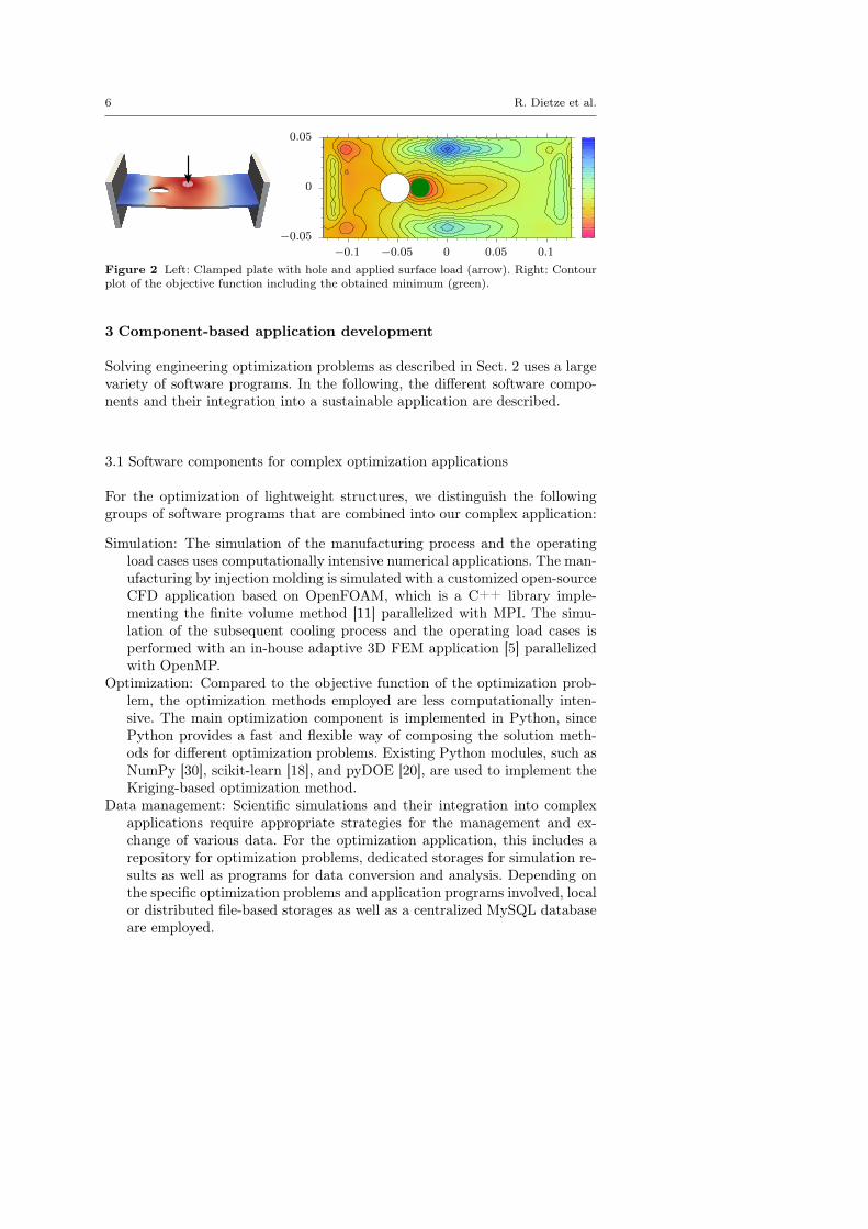
As an example for the optimization of lightweight structures, we considerthe determination of an optimal injection position for the manufacturing of apart made of short fiber-reinforced plastics. Figure 2 (left) shows a plastic part,which is a plate with a hole on one side. The plate is clamped on two sidesand a circular surface load is applied leading to the shown deflection in forcedirection. Figure 2 (right) shows a contour plot of the objective function forthe corresponding optimization problem. The optimal injection point shownin the figure leads to a fiber orientation within the plate that minimizes thedeflection.

6 R. Dietze et al.

−0.05

0

0.05

−0.1 −0.05 0 0.05 0.1

Figure 2 Left: Clamped plate with hole and applied surface load (arrow). Right: Contourplot of the objective function including the obtained minimum (green).

3 Component-based application development

Solving engineering optimization problems as described in Sect. 2 uses a largevariety of software programs. In the following, the different software compo-nents and their integration into a sustainable application are described.

3.1 Software components for complex optimization applications

For the optimization of lightweight structures, we distinguish the followinggroups of software programs that are combined into our complex application:

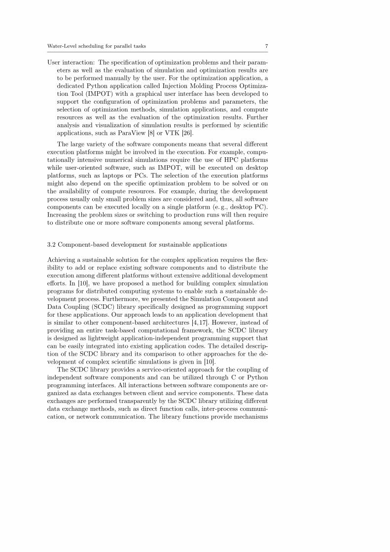
Simulation: The simulation of the manufacturing process and the operatingload cases uses computationally intensive numerical applications. The man-ufacturing by injection molding is simulated with a customized open-sourceCFD application based on OpenFOAM, which is a C++ library imple-menting the finite volume method [11] parallelized with MPI. The simu-lation of the subsequent cooling process and the operating load cases isperformed with an in-house adaptive 3D FEM application [5] parallelizedwith OpenMP.

Optimization: Compared to the objective function of the optimization prob-lem, the optimization methods employed are less computationally inten-sive. The main optimization component is implemented in Python, sincePython provides a fast and flexible way of composing the solution meth-ods for different optimization problems. Existing Python modules, such asNumPy [30], scikit-learn [18], and pyDOE [20], are used to implement theKriging-based optimization method.

Data management: Scientific simulations and their integration into complexapplications require appropriate strategies for the management and ex-change of various data. For the optimization application, this includes arepository for optimization problems, dedicated storages for simulation re-sults as well as programs for data conversion and analysis. Depending onthe specific optimization problems and application programs involved, localor distributed file-based storages as well as a centralized MySQL databaseare employed.


User interaction: The specification of optimization problems and their param-eters as well as the evaluation of simulation and optimization results areto be performed manually by the user. For the optimization application, adedicated Python application called Injection Molding Process Optimiza-tion Tool (IMPOT) with a graphical user interface has been developed tosupport the configuration of optimization problems and parameters, theselection of optimization methods, simulation applications, and computeresources as well as the evaluation of the optimization results. Furtheranalysis and visualization of simulation results is performed by scientificapplications, such as ParaView [8] or VTK [26].

The large variety of the software components means that several differentexecution platforms might be involved in the execution. For example, compu-tationally intensive numerical simulations require the use of HPC platformswhile user-oriented software, such as IMPOT, will be executed on desktopplatforms, such as laptops or PCs. The selection of the execution platformsmight also depend on the specific optimization problem to be solved or onthe availability of compute resources. For example, during the developmentprocess usually only small problem sizes are considered and, thus, all softwarecomponents can be executed locally on a single platform (e. g., desktop PC).Increasing the problem sizes or switching to production runs will then requireto distribute one or more software components among several platforms.

3.2 Component-based development for sustainable applications

Achieving a sustainable solution for the complex application requires the flex-ibility to add or replace existing software components and to distribute theexecution among different platforms without extensive additional developmentefforts. In [10], we have proposed a method for building complex simulationprograms for distributed computing systems to enable such a sustainable de-velopment process. Furthermore, we presented the Simulation Component andData Coupling (SCDC) library specifically designed as programming supportfor these applications. Our approach leads to an application development thatis similar to other component-based architectures [4,17]. However, instead ofproviding an entire task-based computational framework, the SCDC libraryis designed as lightweight application-independent programming support thatcan be easily integrated into existing application codes. The detailed descrip-tion of the SCDC library and its comparison to other approaches for the de-velopment of complex scientific simulations is given in [10].

The SCDC library provides a service-oriented approach for the coupling ofindependent software components and can be utilized through C or Pythonprogramming interfaces. All interactions between software components are or-ganized as data exchanges between client and service components. These dataexchanges are performed transparently by the SCDC library utilizing differentdata exchange methods, such as direct function calls, inter-process communi-cation, or network communication. The library functions provide mechanisms

8 R. Dietze et al.

IMPOT

CFD

Storage Scheduling

FEM

(1)(2) (3)(4)

(5) (6)(7)Client/service

Client accessto service

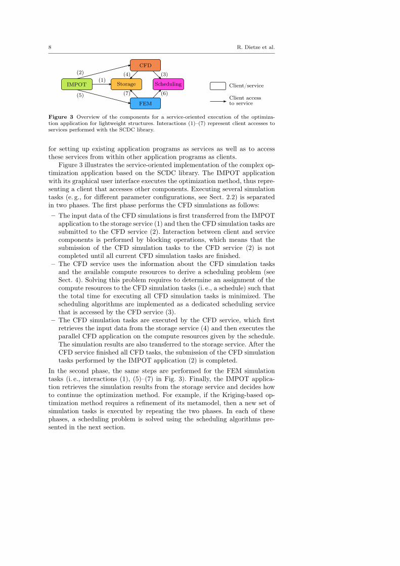
Figure 3 Overview of the components for a service-oriented execution of the optimiza-tion application for lightweight structures. Interactions (1)–(7) represent client accesses toservices performed with the SCDC library.

for setting up existing application programs as services as well as to accessthese services from within other application programs as clients.

Figure 3 illustrates the service-oriented implementation of the complex op-timization application based on the SCDC library. The IMPOT applicationwith its graphical user interface executes the optimization method, thus repre-senting a client that accesses other components. Executing several simulationtasks (e. g., for different parameter configurations, see Sect. 2.2) is separatedin two phases. The first phase performs the CFD simulations as follows:– The input data of the CFD simulations is first transferred from the IMPOT

application to the storage service (1) and then the CFD simulation tasks aresubmitted to the CFD service (2). Interaction between client and servicecomponents is performed by blocking operations, which means that thesubmission of the CFD simulation tasks to the CFD service (2) is notcompleted until all current CFD simulation tasks are finished.

– The CFD service uses the information about the CFD simulation tasksand the available compute resources to derive a scheduling problem (seeSect. 4). Solving this problem requires to determine an assignment of thecompute resources to the CFD simulation tasks (i. e., a schedule) such thatthe total time for executing all CFD simulation tasks is minimized. Thescheduling algorithms are implemented as a dedicated scheduling servicethat is accessed by the CFD service (3).

– The CFD simulation tasks are executed by the CFD service, which firstretrieves the input data from the storage service (4) and then executes theparallel CFD application on the compute resources given by the schedule.The simulation results are also transferred to the storage service. After theCFD service finished all CFD tasks, the submission of the CFD simulationtasks performed by the IMPOT application (2) is completed.

In the second phase, the same steps are performed for the FEM simulationtasks (i. e., interactions (1), (5)–(7) in Fig. 3). Finally, the IMPOT applica-tion retrieves the simulation results from the storage service and decides howto continue the optimization method. For example, if the Kriging-based op-timization method requires a refinement of its metamodel, then a new set ofsimulation tasks is executed by repeating the two phases. In each of thesephases, a scheduling problem is solved using the scheduling algorithms pre-sented in the next section.


4 Scheduling parallel tasks on heterogeneous HPC platforms

The scheduling problem emerging when simulating lightweight structures andseveral scheduling methods for utilizing heterogeneous HPC clusters are pre-sented in the following.

4.1 Scheduling problem for independent parallel tasks

Independent numerical simulations are given as nT parallel tasks T1, . . . , TnT.

The parallel runtime ti(p) of the tasks Ti, i = 1, . . . , nT is assumed to bepreviously determined with benchmark measurements on a specific referencecompute node where p denotes the number of cores employed. It is also as-sumed that it is known whether a task is capable of being executed either ona single node only (SN task, e. g., for OpenMP-based codes) or on a cluster ofnodes (CN task, e. g., for MPI-based codes).

The compute resources of the heterogeneous HPC platform are describedby a machine model with nN compute nodes N1, . . . , NnN

. For each node Nj ,j ∈ {1, . . . , nN}, its number of processor cores pj and a performance factorfj is given. The performance factor fj defines the computational speed ofcompute node Nj as the ratio of the sequential execution time of a task on thereference compute node and on the compute node Nj . The nodes are groupedinto nC clusters C1, . . . , CnC

such that each cluster is a subset of nodes andeach node is part of exactly one cluster. Each cluster is able to execute a CNtask in parallel (e. g., MPI-based) on all its nodes.

A schedule for the tasks Ti, i = 1, . . . , nT to be executed on the computenodes Nj , j = 1, . . . , nN is given by the following information for each task Ti:

– the set of compute nodes and their numbers of cores to be utilized,– the estimated start time si and finish time ei.

The makespan of a schedule is then defined as the time difference betweenthe earliest start time of all tasks and the latest finish time of all tasks. Weassume that the earliest start time is 0 and, thus, the makespan is equal tomaxi=1,...,nT

ei. The goal is to determine a schedule such that the makespan isminimized. Furthermore, we will also determine all tasks that are immediatepredecessors of a task and executed on the same compute node. With thisinformation, it will be possible to wait for the completion of the predecessortasks, especially if the runtimes in practice differ from the estimated runtimes.

4.2 Task and data parallel executions

The following task and data parallel schemes [7] are used as reference methods:

Pure Task Parallel (TaskP): The task parallel scheduling scheme for in-dependent parallel tasks is defined to be a scheme in which exactly onecore is assigned to each task (i. e., executed sequentially). This leads to an

10 R. Dietze et al.

Time MakespanMakespan

CoreCore1 2 3 4 5 6 1 2 3 4 5 6

Time

Figure 4 Scheduling of one task (yellow) either on two (left) or three (right) cores withpreviously scheduled tasks (gray) and optimally executed remaining tasks (blue).

execution of as many tasks as possible at the same time in parallel to eachother.

Pure Data Parallel (DataP): The data parallel scheduling scheme for in-dependent parallel tasks is defined to be a scheme in which as many coresas possible are assigned to each task. Depending on the properties of thetasks (i. e., SN or CN task, see Sect. 4.1), either all cores of a node or allcores of a cluster are used.

The scheduling is performed by iterating over the tasks and selecting thecompute resources to be utilized according to the task parallel or data parallelscheme. To favor an early execution of long running tasks, the tasks are firstsorted in descending order based on their sequential runtimes. A single task isthen assigned to the compute resource that provides the earliest finish. Bothschemes are adapted to heterogeneous compute resources by scaling the givenruntimes of the tasks with the performance factors of the compute nodes.

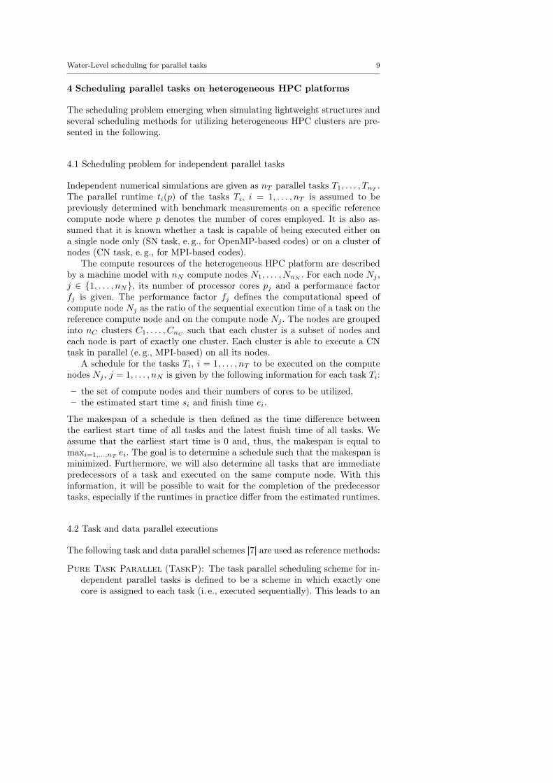
4.3 Water-Level method

We propose a new scheduling strategy which we call Water-Level method(WaterL). For each task, the Water-Level method selects the computenodes and the number of cores for which an estimation of the resulting makespanreaches a minimum. This estimation is determined by assigning a task tem-porarily to specific compute nodes and cores and assuming all remaining tasksare executed fully parallel without parallelization overhead on the entire set ofcompute resources. Figure 4 shows an illustration of the Water-Level strat-egy in which the current task to be scheduled (yellow) will use either two (left)or three (right) cores. All tasks that are not scheduled yet (blue) are assumedto be executed fully parallel on all cores (i. e., they are distributed like “water”over the “task landscape”). In this example, the current task will be assignedto three cores since the estimation of the resulting makespan (i. e., the “waterlevel”) reaches a minimum.

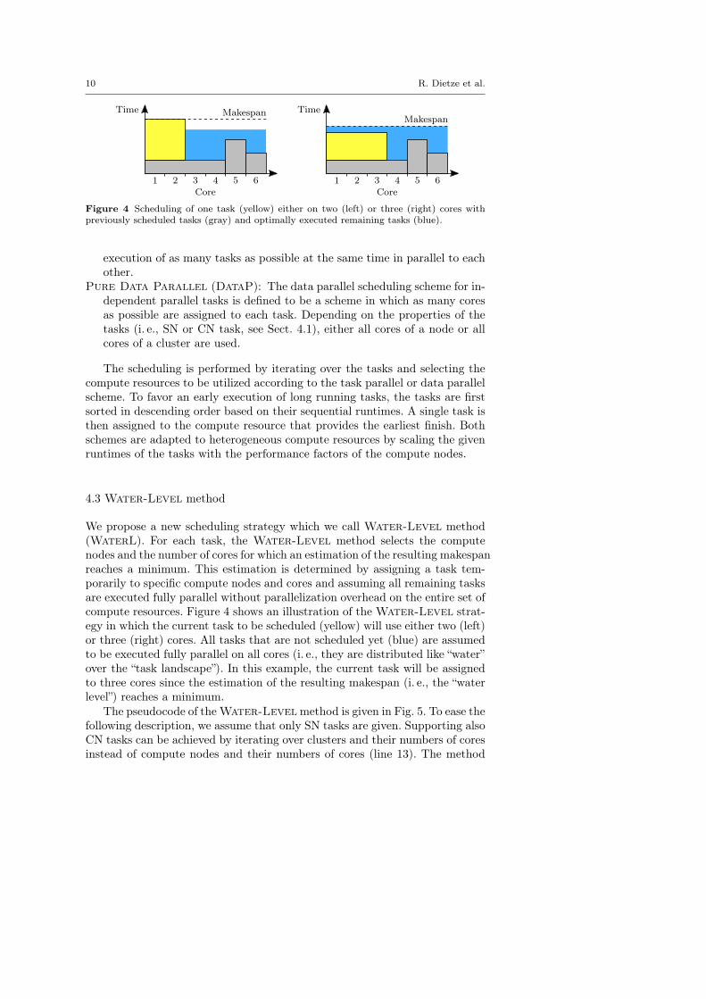
The pseudocode of the Water-Level method is given in Fig. 5. To ease thefollowing description, we assume that only SN tasks are given. Supporting alsoCN tasks can be achieved by iterating over clusters and their numbers of coresinstead of compute nodes and their numbers of cores (line 13). The method


1 input : tasks Ti, i = 1, . . . , nT , with runtimes ti(p)2 input : nodes Nj , j = 1, . . . , nN , with pj cores and performance factors fj3 output: compute node, number of cores, start time and finish time for each task4 total compute power P =

∑nNj=1 pj · fj

5 sequential work WS =∑nT

i=1 ti(1)6 free work WF = 07 latest finish time emax = 08 sort Ti, i = 1, . . . , nT in descending order of ti(1)9 // assume T1, . . . , TnT are sorted in descending order of their sequential runtimes

10 for i = 1, . . . , nT do11 WS =WS − ti(1)12 best estimated makespan m∗ =∞13 for j = 1, . . . , nN and p = 1, . . . , pj do14 assign Ti temporarily to p cores of compute node Nj

15 s = start time of task Ti16 e = s+ ti(p)/fj17 dWF = (max(e, emax)− emax) · P18 dWF = dWF − (e− s) · fj · p19 estimated makespan m = max(e, emax)20 if WS > WF + dWF then m = m+ WS−(WF+dWF )/P21 if m < m∗ then { (m∗, j∗, p∗, s∗, e∗, dW ∗

F ) = (m, j, p, s, e, dWF ) }

22 assign p∗ cores of node Nj∗ to task Ti with start time s∗ and finish time e∗23 WF =WF + dW ∗

F24 emax = max(e∗, emax)

Figure 5 Pseudocode of the Water-Level scheduling method.

starts by calculating the total compute power P of all compute nodes withrespect to a single core of the reference compute node (line 4). The sequentialwork WS is determined as the work for executing all tasks sequentially onthe reference compute node (line 5). Additionally, the free work WF and thelatest finish time of all tasks emax are initialized (lines 6 and 7). While emax

corresponds to the makespan of the determined schedule, the free work WF

is equal to amount of work that can be executed by all compute resourceswithout increasing this makespan.

The determination of a schedule of the tasks proceeds as follows. The tasksare sorted in descending order based on their sequential runtimes (line 8) anda loop iterates over all tasks in that sorted order (line 10). For the currenttask Ti, i ∈ {1, . . . , nT }, the remaining sequential work WS of all unscheduledtasks is calculated (line 11). The currently best estimated makespanm∗ that isachieved for scheduling the task Ti is initialized in such a way (line 12) that itis larger than the following estimation. Then, a loop iterates over the computenodes and their numbers of cores (line 13) to determine the compute node andthe number of cores to be assigned for the task Ti.

The current task Ti is temporarily assigned to the currently considered pcores of compute node Nj (line 14), thus leading to a potential start time s(line 15). The potential finish time e is then calculated from the parallel run-time ti(p) of the task scaled with the performance factor fj of the currentlyconsidered compute node Nj (line 16). Estimating the makespan for this as-

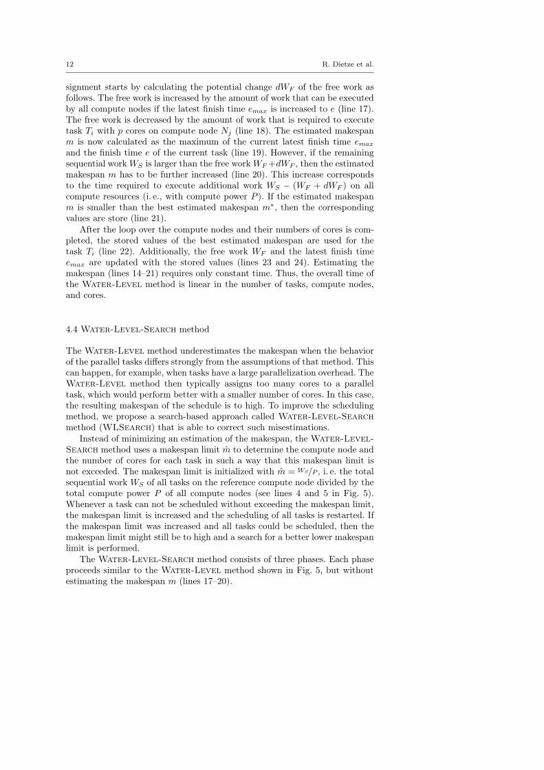
12 R. Dietze et al.

signment starts by calculating the potential change dWF of the free work asfollows. The free work is increased by the amount of work that can be executedby all compute nodes if the latest finish time emax is increased to e (line 17).The free work is decreased by the amount of work that is required to executetask Ti with p cores on compute node Nj (line 18). The estimated makespanm is now calculated as the maximum of the current latest finish time emax

and the finish time e of the current task (line 19). However, if the remainingsequential workWS is larger than the free workWF +dWF , then the estimatedmakespan m has to be further increased (line 20). This increase correspondsto the time required to execute additional work WS − (WF + dWF ) on allcompute resources (i. e., with compute power P ). If the estimated makespanm is smaller than the best estimated makespan m∗, then the correspondingvalues are store (line 21).

After the loop over the compute nodes and their numbers of cores is com-pleted, the stored values of the best estimated makespan are used for thetask Ti (line 22). Additionally, the free work WF and the latest finish timeemax are updated with the stored values (lines 23 and 24). Estimating themakespan (lines 14–21) requires only constant time. Thus, the overall time ofthe Water-Level method is linear in the number of tasks, compute nodes,and cores.

4.4 Water-Level-Search method

The Water-Level method underestimates the makespan when the behaviorof the parallel tasks differs strongly from the assumptions of that method. Thiscan happen, for example, when tasks have a large parallelization overhead. TheWater-Level method then typically assigns too many cores to a paralleltask, which would perform better with a smaller number of cores. In this case,the resulting makespan of the schedule is to high. To improve the schedulingmethod, we propose a search-based approach called Water-Level-Searchmethod (WLSearch) that is able to correct such misestimations.

Instead of minimizing an estimation of the makespan, the Water-Level-Search method uses a makespan limit m̂ to determine the compute node andthe number of cores for each task in such a way that this makespan limit isnot exceeded. The makespan limit is initialized with m̂ = WS/P , i. e. the totalsequential work WS of all tasks on the reference compute node divided by thetotal compute power P of all compute nodes (see lines 4 and 5 in Fig. 5).Whenever a task can not be scheduled without exceeding the makespan limit,the makespan limit is increased and the scheduling of all tasks is restarted. Ifthe makespan limit was increased and all tasks could be scheduled, then themakespan limit might still be to high and a search for a better lower makespanlimit is performed.

The Water-Level-Search method consists of three phases. Each phaseproceeds similar to the Water-Level method shown in Fig. 5, but withoutestimating the makespan m (lines 17–20).


Phase 1: The loop over the compute nodes and their numbers of cores (line 13)is stopped if the potential finish time e is less than or equal to the makespanlimit m̂. In this case, the current compute node and cores are assigned tothe current task and the next task is scheduled. If the makespan limit m̂is exceeded by all finish times e, then the makespan limit is set to thesmallest finish time and the scheduling of all tasks is potentially restarted.More specifically, the restarts are only performed after nT

2 , 3nT

4 , 7nT

8 , . . .tasks to limit the number of restarts to O(log nT ).

Phase 2: Since the last makespan limit m̂ might still be to large, a binarysearch for a smaller makespan limit is performed. A list of candidates forthe search is created by collecting all finish times e during an executionof the algorithm shown in Fig. 5. The resulting number of candidates islimited to nT

∑nN

j=1 pj .Phase 3: The binary search is performed as long as there are candidates left for

the makespan limit. In each step of the search, the median of the candidatesis used as the makespan limit m̂ to perform the algorithm shown in Fig. 5in the same way as in Phase 1. Depending on whether the makespan limitis exceeded or not, the candidates below or above the median are removed.Finally, the last remaining candidate is used as the makespan limit thatleads to the schedule determined by the Water-Level-Search method.

Each phase performs the algorithm shown in Fig. 5 one or several times.The total number of repetitions depends logarithmically on the number oftasks and the total number of cores.

5 Performance results of the scheduling methods

In this section, we present performance results of the scheduling methods de-scribed in Sect. 4 on a heterogeneous compute cluster.

5.1 Experimental setup

The heterogeneous compute cluster used consists of nN = 8 compute nodes,each with two multi-core processors. Table 1 lists the nodes and their specificprocessors. The compute node cs1 is used as the reference compute node andthe performance factors of all other compute nodes are calculated as the ratioof the corresponding sequential execution times of the tasks (see Sect. 4.1).The scheduling methods described in Sect. 4 are implemented in Python. Addi-tionally, we have implemented two methods that represent existing approachesfor the scheduling of parallel tasks on heterogeneous compute clusters:

HCPA: The Heterogeneous Critical Path and Allocation method [15]transforms individual computational speeds of processors into additional“virtual” processors with equal speed. The scheduling is then performedwith an existing method for homogeneous compute clusters (i. e., CPA [22]).

14 R. Dietze et al.

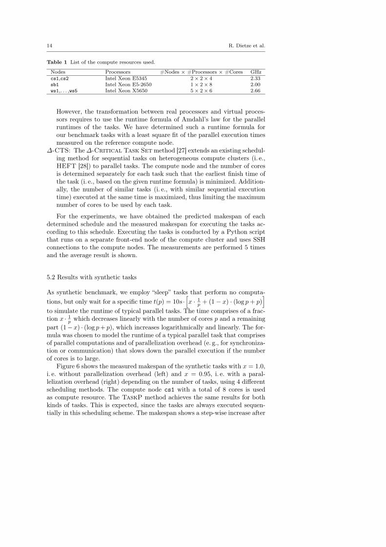
Table 1 List of the compute resources used.

Nodes Processors #Nodes × #Processors × #Cores GHzcs1,cs2 Intel Xeon E5345 2× 2× 4 2.33sb1 Intel Xeon E5-2650 1× 2× 8 2.00ws1,. . . ,ws5 Intel Xeon X5650 5× 2× 6 2.66

However, the transformation between real processors and virtual proces-sors requires to use the runtime formula of Amdahl’s law for the parallelruntimes of the tasks. We have determined such a runtime formula forour benchmark tasks with a least square fit of the parallel execution timesmeasured on the reference compute node.

∆-CTS: The∆-Critical Task Set method [27] extends an existing schedul-ing method for sequential tasks on heterogeneous compute clusters (i. e.,HEFT [28]) to parallel tasks. The compute node and the number of coresis determined separately for each task such that the earliest finish time ofthe task (i. e., based on the given runtime formula) is minimized. Addition-ally, the number of similar tasks (i. e., with similar sequential executiontime) executed at the same time is maximized, thus limiting the maximumnumber of cores to be used by each task.

For the experiments, we have obtained the predicted makespan of eachdetermined schedule and the measured makespan for executing the tasks ac-cording to this schedule. Executing the tasks is conducted by a Python scriptthat runs on a separate front-end node of the compute cluster and uses SSHconnections to the compute nodes. The measurements are performed 5 timesand the average result is shown.

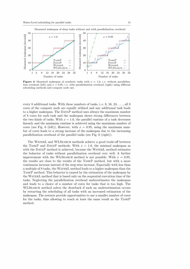
5.2 Results with synthetic tasks

As synthetic benchmark, we employ “sleep” tasks that perform no computa-tions, but only wait for a specific time t(p) = 10s ·

[x · 1p + (1− x) · (log p+ p)

]to simulate the runtime of typical parallel tasks. The time comprises of a frac-tion x · 1p which decreases linearly with the number of cores p and a remainingpart (1− x) · (log p+ p), which increases logarithmically and linearly. The for-mula was chosen to model the runtime of a typical parallel task that comprisesof parallel computations and of parallelization overhead (e. g., for synchroniza-tion or communication) that slows down the parallel execution if the numberof cores is to large.

Figure 6 shows the measured makespan of the synthetic tasks with x = 1.0,i. e. without parallelization overhead (left) and x = 0.95, i. e. with a paral-lelization overhead (right) depending on the number of tasks, using 4 differentscheduling methods. The compute node cs1 with a total of 8 cores is usedas compute resource. The TaskP method achieves the same results for bothkinds of tasks. This is expected, since the tasks are always executed sequen-tially in this scheduling scheme. The makespan shows a step-wise increase after


0

10

20

30

40

50

1 4 8 12 16 20 24 28 32

x = 1.0

0

10

20

30

40

50

1 4 8 12 16 20 24 28 32

x = 0.95

Measuredmak

espa

n[secon

ds]

Number of tasks

Measured makespan of sleep tasks without and with parallelization overhead

TaskPDataPWaterLWLSearch M

easuredmak

espa

n[secon

ds]

Number of tasks

TaskPDataPWaterLWLSearch

Figure 6 Measured makespan of synthetic tasks with x = 1.0, i. e. without paralleliza-tion overhead (left) and x = 0.95, i. e. with parallelization overhead (right) using differentscheduling methods and compute node cs1.

every 8 additional tasks. With these numbers of tasks, i. e. 8, 16, 24, . . . , all 8cores of the compute node are equally utilized and any additional task leadsto a higher makespan. The DataP method uses always the maximum numberof 8 cores for each task and the makespan shows strong differences betweenthe two kinds of tasks. With x = 1.0, the parallel runtime of a task decreaseslinearly and the minimum runtime is achieved using the maximum number ofcores (see Fig. 6 (left)). However, with x = 0.95, using the maximum num-ber of cores leads to a strong increase of the makespan due to the increasingparallelization overhead of the parallel tasks (see Fig. 6 (right)).

The WaterL and WLSearch methods achieve a good trade-off betweenthe TaskP and DataP methods. With x = 1.0, the minimal makespan aswith the DataP method is achieved, because the WaterL method estimatesthe behavior of tasks without parallelization overhead very well. A furtherimprovement with the WLSearch method is not possible. With x = 0.95,the results are close to the results of the TaskP method, but with a morecontinuous increase instead of the step-wise increase. Especially with less thana multiple of 8 tasks, the WaterL method leads to a higher makespan than theTaskP method. This behavior is caused by the estimation of the makespan bythe WaterL method that is based only on the sequential execution time of thetasks. Neglecting the parallelization overhead underestimates the makespanand leads to a choice of a number of cores for tasks that is too high. TheWLSearch method solves the drawback if such an underestimation occursby restarting the scheduling of all tasks with an increased estimation of themakespan. The restarts provide opportunities to use a smaller number of coresfor the tasks, thus allowing to reach at least the same result as the TaskPmethod.

16 R. Dietze et al.

0

10

20

30

40

50

1 4 8 12 16 20 24 28 32 36 400

10

20

30

40

50

1 4 8 12 16 20 24 28 32 36 40

Estim

ated

mak

espa

n[secon

ds]

Number of tasks

Predicted and measured makespan of DGEMM tasks

TaskPDataPHCPA∆-CTSWaterLWLSearch

Measuredmak

espa

n[secon

ds]

Number of tasks


Figure 7 Predicted makespan (left) and measured makespan (right) of DGEMM tasksusing different scheduling methods and compute nodes cs1 and ws1.

5.3 Results with DGEMM tasks

The number of cores utilized by the DGEMM operation of the OpenBLASlibrary is controlled with the environment variable OPENBLAS_NUM_THREADS.The parallel runtime of a DGEMM task using p cores is modeled with theruntime formula t(p) = a/pb + c. The parameters a, b, and c are determinedwith a least square fit (by Gnuplot) of the parallel execution times measuredon the reference compute node cs1. The resulting runtime with matrices of size4000× 4000 comprises of a constant part c = 2.30 seconds and a parallel parta = 13.09 seconds that decreases proportionally to 1/p1.09. Thus, even thoughthe parallel part scales very well, there is always a significant sequential part.

Figure 7 (left) shows the predicted makespan of DGEMM tasks dependingon the number of tasks, using 6 different scheduling methods. The two computenodes cs1 and ws1 with a total of 20 cores are used as compute resources.Similar to Fig. 6 (left), the TaskP method shows a step-wise increase of theexecution times due to the sequential execution of the tasks while the DataPmethod shows a strong increase due to the parallelization overhead caused byalways using the maximum number of cores. The existing methods HCPA and∆-CTS lead to an improved makespan for small numbers of tasks. However,if the number of tasks is larger than the total number of cores, then the samestep-wise increase as the TaskP method occurs. In this case, only one core isassigned to each task, because both methods chose the maximum number ofcores to be assigned to a task without considering the potential utilization ofcores by other tasks.

The WaterL method leads to a continuous increase of the makespan for in-creasing numbers of tasks. Furthermore, the makespan of the WaterL methodis always below or at most equal to the best results of the TaskP method. Thisis the expected behavior, because the estimation of the makespan that is usedto determine the number of cores to be assigned to a task represents a predic-


tion of the remaining utilization of the cores. If there are many tasks left, thenthis utilization is high and a task parallel execution is preferred. Otherwise, thepredicted utilization is low and a data parallel execution of the few remainingtasks is chosen. The results demonstrate this intended trade-off between taskand data parallel executions. However, due to the significant sequential partwithin the parallel DGEMM task, the WaterL method also underestimatesthe makespan. By repeatedly improving the estimation of the makespan, theWLSearch method further improves the makespan of the WaterL methodby about 6% on average.

Figure 7 (right) shows the measured makespan achieved by executing theDGEMM tasks according to the determined schedule. The results of the DataPmethod are close to the predicted makespan (left), but still lead to the high-est makespan results. All other methods lead to strongly varying results. Thisbehavior is caused by the DGEMM tasks which influence each other whenexecuted on the same compute node. Due to the significant sequential part ofthe tasks, all methods except the DataP method prefer the execution of mul-tiple tasks at once. However, especially the step-wise increase of the TaskP,HCPA, and ∆-CTS methods is still visible. The majority of the smallest mea-sured makespans is achieved with the WLSearch method, thus confirmingthe results of the predicted makespan (left).

5.4 Results with FEM simulation tasks

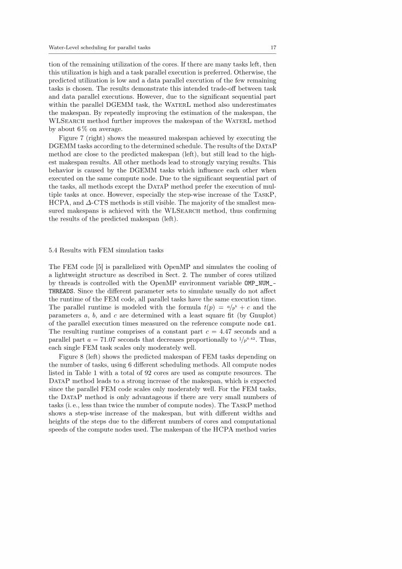
The FEM code [5] is parallelized with OpenMP and simulates the cooling ofa lightweight structure as described in Sect. 2. The number of cores utilizedby threads is controlled with the OpenMP environment variable OMP_NUM_-THREADS. Since the different parameter sets to simulate usually do not affectthe runtime of the FEM code, all parallel tasks have the same execution time.The parallel runtime is modeled with the formula t(p) = a/pb + c and theparameters a, b, and c are determined with a least square fit (by Gnuplot)of the parallel execution times measured on the reference compute node cs1.The resulting runtime comprises of a constant part c = 4.47 seconds and aparallel part a = 71.07 seconds that decreases proportionally to 1/p0.42. Thus,each single FEM task scales only moderately well.

Figure 8 (left) shows the predicted makespan of FEM tasks depending onthe number of tasks, using 6 different scheduling methods. All compute nodeslisted in Table 1 with a total of 92 cores are used as compute resources. TheDataP method leads to a strong increase of the makespan, which is expectedsince the parallel FEM code scales only moderately well. For the FEM tasks,the DataP method is only advantageous if there are very small numbers oftasks (i. e., less than twice the number of compute nodes). The TaskP methodshows a step-wise increase of the makespan, but with different widths andheights of the steps due to the different numbers of cores and computationalspeeds of the compute nodes used. The makespan of the HCPA method varies

18 R. Dietze et al.

0

50

100

150

200

250

300

350

1 20 40 60 80 100 1200

50

100

150

200

250

300

350

1 20 40 60 80 100 120

Estim

ated

mak

espa

n[secon

ds]

Number of tasks

Predicted and measured makespan of FEM simulation tasks


Measuredmak

espa

n[secon

ds]

Number of tasks


Figure 8 Predicted makespan (left) and measured makespan (right) of FEM tasks usingdifferent scheduling methods and all compute nodes listed in Table 1.

around the TaskP method while the makespan of the∆-CTS method is eitherhigher than or equal to the TaskP method.

The makespan of the WaterL method is up to a factor of two higher thanthe TaskP method. This behavior is caused by the FEM code that favors anexecution with small numbers of cores and the fact that the WaterL methodassumes an optimal parallel execution for its estimation of the makespan,which differs strongly from the actual parallel runtimes of the FEM tasks. TheWLSearch method solves this problem by repeating the WaterL methodseveral times with improved estimations of the makespan. In general, this im-provement is especially important for parallel codes that scale only moderatelywell. The resulting makespan of the WLSearch method is always the best incomparison to all other methods.

Figure 8 (right) shows the measured makespan achieved by executing theFEM tasks according to the determined schedules. The results confirm thegeneral behavior of the methods, which was previously seen in the predictedmakespan results, i. e. the WLSearch method achieves the smallest executiontimes for a broad range of numbers of tasks. However, the measured makespanresults are up to about a factor of 1.4 higher with less than 80 tasks and upto a factor of 2 higher for larger numbers of tasks. This strong increase occursif a high number of sequential FEM tasks is executed on single nodes at thesame time. One reason might be that due to the limited memory bandwidth ofthe compute nodes cs1 and cs2, the sequential runtimes of FEM tasks almostdouble if all eight cores execute a separate (sequential) FEM task. However,this affects all scheduling methods that rely on a given runtime formula forthe execution times of the tasks.

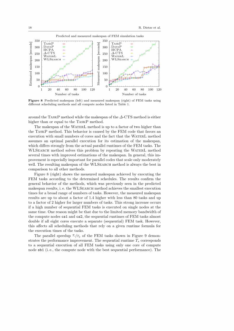
The parallel speedup Ts/Tp of the FEM tasks shown in Figure 9 demon-strates the performance improvement. The sequential runtime Ts correspondsto a sequential execution of all FEM tasks using only one core of computenode sb1 (i. e., the compute node with the best sequential performance). The


1

4

8

12

16

20

24

28

1 8 16 28 40 52 64 76 921

8

16

24

32

40

48

1 8 16 28 40 52 64 76 92

Speedu

p

Number of cores

Measured parallel speedup with FEM simulation tasks


Speedu

p

Number of cores


Figure 9 Parallel speedup achieved for the execution of 16 (left) and 92 (right) FEM tasksusing different scheduling methods.

parallel runtime Tp corresponds to a parallel execution of all FEM tasks basedon a schedule determined for using compute nodes with a total number of pcores. Increasing the number of cores utilizes the compute nodes in order oftheir performance, i. e. 1–16 cores with compute node sb1, 28–76 cores withadditional compute nodes ws1–ws5, and 92 cores with all compute nodes listedin Table 1. Thus, the scheduling methods have to handle the heterogeneity ofthe different compute nodes and the varying ratios between the number oftasks and the number of cores.

Figure 9 (left) shows the parallel speedup with 16 FEM tasks dependingon the number of cores, using 6 different scheduling methods. The DataPmethod always leads to the lowest speedup results, thus demonstrating theneed for an appropriate scheduling of the FEM tasks in favor of the parallelexecution of the FEM application itself. Up to 16 cores, all methods exceptthe DataP method, assign the 16 cores of compute node sb1 equally to thetasks, thus leading to the same results. However, especially with 16 cores, theparallel speedup of about 12 is lower than expected for executing all 16 taskssequentially at the same time. This is caused by an increase of the sequentialexecution times if several FEM tasks are executed on a single compute node,as mentioned before.

Using more than 16 cores leads to varying speedups for the different schedul-ing methods. The speedup of the TaskP method remains constant, becauseall 16 tasks are executed sequentially on the 16 cores of the compute nodesb1 and additional compute nodes are not used. The speedup of the HCPAmethod and the WaterL method decreases with 28 cores and increases onlyslightly when using additional cores. Both methods assign too many cores tosingle tasks based on an expected parallel behavior (i. e., Amdahl-like or water-like), which differs strongly from their actual parallel execution. The ∆-CTSmethod does not experience these effects, because it prevents an unbalancedassignment of cores to tasks. However, the balancing ignores the different com-

20 R. Dietze et al.

putational speeds of the processors, thus leading to a strong decrease of thespeedup when additionally using the slow compute nodes cs1 and cs2. TheWLSearch method achieves an increasing speedup up to 92 cores. The prob-lematic assignment of too many cores to single tasks is resolved by repeatingthe assignment of cores to tasks with improved estimations of the makespan.Furthermore, using slower computes nodes does not deteriorate the speedup,because the assignment is based on the parallel runtime of the tasks recogniz-ing also the different computational speeds of the processors.

Figure 9 (right) shows the parallel speedup with 92 FEM tasks dependingon the number of cores, using 6 different scheduling methods. In comparisonto the results with 16 FEM tasks, all scheduling methods, except the DataPmethod, achieve a significant speedup with more than 16 cores. This is theexpected behavior when using less cores than tasks, because in these cases theadditional cores are used to execute more tasks sequentially at the same time.Using 92 cores leads to a significant decrease of the speedup for the TaskPmethod and the ∆-CTS method. In this case, both methods execute all taskssequentially and the slow compute nodes cs1 and cs2 decrease the overallspeedup. Especially, the WLSearch method achieves a further increase whenusing all 92 cores, thus confirming the good results that were already shownwith less tasks (left).

In comparison to the DGEMM tasks used in the previous subsection, theparallel behavior of the FEM simulation tasks has shown to be very challengingfor the scheduling methods. The usage of slow compute nodes as well as caseswith less tasks than cores affect the efficiency of most of the scheduling methodssuch that their results are often not better than the task parallel scheme. Incontrast to that, the WLSearch method has demonstrated consistently goodresults in all these cases, thus showing that both benchmark tasks and realisticapplication tasks can be handled appropriately.

6 Related Work

Scheduling is an important problem supporting the efficient processing in dif-ferent application areas [19]. One prominent area is the scheduling of sequentialand/or parallel tasks to be executed on a given set of hardware resources (e. g.,cores, processors, or nodes) while additional dependencies between the tasksmay restrict their execution order. Determining an optimal schedule (e. g., withminimal makespan) for tasks with dependencies is an NP-hard problem that isusually solved with heuristics or approximation algorithms [13]. Layer-basedscheduling algorithms [23] decompose a set of parallel tasks with dependen-cies into layers of independent tasks. Each layer is scheduled separately with ascheduling algorithm for independent tasks, e. g. list scheduling. Since the sim-ulation tasks of our optimization application are independent, a decompositioninto layers can be omitted.

List scheduling algorithms add priorities to the tasks and assign the tasksin descending order of their priority to the processors. Algorithms, such as


Largest Processing Time (LPT) [3] and Longest Task First (LTF) [29],use the given runtime of the tasks as priorities to assign compute intensivetasks first. Algorithms for heterogeneous platforms, such as HeterogeneousEarliest Finish Time (HEFT) [28] and Predict Earliest Finish Time(PEFT) [1], also take the runtime of the tasks on individual processors intoaccount for the priorities. The Water-Level method proposed in this articleis also a list scheduling algorithm that prioritizes the tasks according to theirruntime. However, the Water-Level method uses only the sequential runtimeas priority while the individual processor speeds of a heterogeneous platformare used for the allocation of cores to parallel tasks and for the selection ofcompute nodes.

Scheduling parallel tasks can also be performed with a two-step approachconsisting of an allocation step followed by a scheduling step. The schedulingstep assigns the parallel tasks to specific processors and is usually based on alist scheduling algorithm. The allocation step determines the number of pro-cessors for each parallel task. This step is usually performed iteratively startingwith an initial allocation (e. g., one processor per tasks) and then repeatedlyassigning additional processors to tasks (e. g., to shorten the critical path).The resulting number of repetitions depends linearly on the number of tasks.Example algorithms are Critical Path Reduction (CPR) [21], CriticalPath and Allocation (CPA) [22], and Modified Critical Path andArea-based (MCPA) [2]. The Water-Level method performs the alloca-tion of cores only once for each task during the list scheduling and, thus, omitsrepeated assignments of additional processors to tasks. The Water-Level-Search method repeats the Water-Level method, but with a number ofrepetitions that depends only logarithmically on the number of tasks.

The HCPA method [15] is an extension of the CPA method and requiresto calculate the parallel runtime of tasks according to Amdahl’s law (seeSect. 5.1). In contrast, both the WaterL method and the WLSearch use thegiven parallel runtime of the tasks, thus omitting such limitations to a specificruntime formula. The ∆-Critical Task Set method (∆-CTS) [27] repre-sents an extension of the HEFT method for parallel tasks and, thus, uses theearliest finish time according the given parallel runtime (see Sect. 5.1). Thisis also done by the Water-Level method. However, the ∆-CTS methodconsiders only subsets of tasks together (i. e., tasks within a specific rangeof the so-called bottom level) while the Water-Level method always con-siders all tasks. Furthermore, the Water-Level-Search method iterativelyimproves the schedule in several steps while the ∆-CTS method performs onlyone step. Especially for the FEM simulation tasks from our complex applica-tion, the experiments in Sect. 5 have demonstrated that these advantages ofthe WLSearch method lead to a smaller makespan and to better parallelspeedup results than the HCPA method and the ∆-CTS method and, thus,the WLSearch method outperforms the other methods.

22 R. Dietze et al.

7 Conclusion

In this article, we have described a component-based development of a com-plex scientific application from the area of engineering optimization and haveshown that a scheduling problem arises, which has to be solved efficiently foran overall efficient execution. Achieving a sustainable application has beenaccomplished by a flexible development approach that enables both to addor replace individual software components and to distribute their executionamong different platforms. To support this approach, we have proposed twoscheduling methods for the efficient execution of parallel simulation tasks onheterogeneous HPC platforms. The Water-Level method performs an itera-tive assignment of the parallel tasks to compute resources and uses a best-caseestimation of the makespan to determine the number of cores to be assigned totasks. The Water-Level-Search method repeats this assignment with im-proved estimations of the parallel behavior of the tasks. Performance resultsfor benchmark tasks demonstrate that the goal to achieve a good trade-offbetween task and data parallel execution schemes has been reached. In com-parison to other existing scheduling methods for parallel tasks, the Water-Level-Search method leads to consistent good results for both benchmarktasks and realistic application tasks. A significant speedup is also achieved forthe execution of the set of specific FEM simulation tasks from the complexsimulation application considered.

Acknowledgements This work was performed within the Federal Cluster of ExcellenceEXC 1075 “MERGE Technologies for Multifunctional Lightweight Structures” and supportedby the German Research Foundation (DFG). Financial support is gratefully acknowledged.

References

1. Arabnejad, H., Barbosa, J.: List scheduling algorithm for heterogeneous systems by anoptimistic cost table. Transactions on Parallel and Distributed Systems 25(3), 682–694(2014)

2. Bansal, S., Kumar, P., Singh, K.: An improved two-step algorithm for task and dataparallel scheduling in distributed memory machines. Parallel Computing 32(10), 759–774 (2006)

3. Belkhale, K., Banerjee, P.: An approximate algorithm for the partitionable indepen-dent task scheduling problem. In: Proc. of the 1990 Int. Conf. on Parallel Processing,(ICPP’90), pp. 72–75 (1990)

4. Bernholdt, D., Allan, B., Armstrong, R., Bertrand, F., Chiu, K., Dahlgren, T.,Damevski, K., Elwasif, W., Epperly, T., Govindaraju, M., Katz, D., Kohl, J., Krish-nan, M., Kumfert, G., Larson, J., Lefantzi, S., Lewis, M., Malony, A., Mclnnes, L.,Nieplocha, J., Norris, B., Parker, S., Ray, J., Shende, S., Windus, T., Zhou, S.: A com-ponent architecture for high-performance scientific computing. Int. J. High PerformanceComputing Applications 20(2), 163–202 (2006)

5. Beuchler, S., Meyer, A., Pester, M.: SPC-PM3AdH v1.0 - Programmer’s manual.Preprint SFB/393 01-08, TU-Chemnitz (2001)

6. Bongo, L.A., Ciegis, R., Frasheri, N., Gong, J., Kimovski, D., Kropf, P., Margenov,S., Mihajlovic, M., Neytcheva, M., Rauber, T., Rünger, G., Trobec, R., Wuyts, R.,Wyrzykowski, R.: Applications for ultrascale computing. Supercomputing Frontiersand Innovations 2(1), 19–48 (2015)


7. Dümmler, J., Kunis, R., Rünger, G.: A comparison of scheduling algorithms for mul-tiprocessortasks with precedence constraints. In: Proc. of the High Performance Com-puting & Simulation Conference (HPCS’07), pp. 663–669. ECMS (2007)

8. Henderson Squillacote, A.: The ParaView guide: A parallel visualization application.Kitware (2008)

9. Hofmann, M., Ospald, F., Schmidt, H., Springer, R.: Programming support for theflexible coupling of distributed software components for scientific simulations. In: Proc.of the 9th Int. Conf. on Software Engineering and Applications (ICSOFT-EA 2014), pp.506–511. SciTePress (2014)

10. Hofmann, M., Rünger, G.: Sustainability through flexibility: Building complex simula-tion programs for distributed computing systems. Simulation Modelling Practice andTheory, Special Issue on Techniques And Applications For Sustainable Ultrascale Com-puting Systems 58(1), 65–78 (2015)

11. Jasak, H., Jemcov, A., Tukovic, Z.: OpenFOAM: A C++ library for complex physicssimulations. In: Proc. of the Int. Workshop on Coupled Methods in Numerical Dynamics(CMND’07), pp. 1–20 (2007)

12. Kleijnen, J., van Beers, W., van Nieuwenhuyse, I.: Expected improvement in efficientglobal optimization through bootstrapped kriging. J. of Global Optimization 54(1),59–73 (2012)

13. Leung, J. (ed.): Handbook of Scheduling: Algorithms, Models, and Performance Anal-ysis. CRC Press (2004)

14. Montgomery, D.: Design and analysis of experiments, 5 edn. Wiley (2000)15. N’Takpé, T., Suter, F.: Critical path and area based scheduling of parallel task graphs

on heterogeneous platforms. In: Proc. of the 12th Int. Conf. on Parallel and DistributedSystems (ICPADS’06), pp. 1–8. IEEE (2006)

16. OpenBLAS: An optimized BLAS library. http://www.openblas.net/17. Parker, S.: A component-based architecture for parallel multi-physics PDE simulation.

Future Generation Computer Systems 22(1–2), 204–216 (2006)18. Pedregosa, F., Varoquaux, G., Gramfort, A., Michel, V., Thirion, B., Grisel, O., Blondel,

M., Prettenhofer, P., Weiss, R., Dubourg, V., Vanderplas, J., Passos, A., Cournapeau,D., Brucher, M., Perrot, M., Duchesnay, E.: Scikit-learn: Machine learning in Python.J. of Machine Learning Research 12, 2825–2830 (2011)

19. Pinedo, M.: Scheduling: Theory, algorithms, and systems. Springer (2012)20. pyDOE: Design of experiments for Python. http://pythonhosted.org/pyDOE21. Radulescu, A., Nicolescu, C., van Gemund, A., Jonker, P.: CPR: Mixed task and data

parallel scheduling for distributed systems. In: Proc. of the 15th Int. Parallel andDistributed Processing Symposium (IPDPS’01), pp. 1–8. IEEE (2001)

22. Radulescu, A., van Gemund, A.: A low-cost approach towards mixed task and dataparallel scheduling. In: Proc. of the Int. Conf. on Parallel Processing (ICPP’01), pp.69–76. IEEE (2001)

23. Rauber, T., Rünger, G.: Compiler support for task scheduling in hierarchical executionmodels. J. of Systems Architecture 45(6–7), 483–503 (1999)

24. Roux, W., Stander, N., Haftka, R.: Response surface approximations for structuraloptimization. Int. J. for Numerical Methods in Engineering 42(3), 517–534 (1998)

25. Sacks, J., Welch, W., Mitchell, T., Wynn, H.: Design and analysis of computer experi-ments. Statistical science 4(4), 409–423 (1989)

26. Schroeder, W., Martin, K., Lorensen, B.: The Visualization Toolkit: An Object-orientedApproach to 3D Graphics. Kitware (2006)

27. Suter, F.: Scheduling ∆-critical tasks in mixed-parallel applications on a national grid.In: Proc. of the 8th IEEE/ACM Int. Conf. on Grid Computing, pp. 2–9. IEEE (2007)

28. Topcuoglu, H., Hariri, S., Wu, M.Y.: Task scheduling algorithms for heterogeneousprocessors. In: Proc. of the 8th Heterogeneous Computing Workshop (HCW’99), pp.3–14. IEEE (1999)

29. Turek, J., Wolf, J., Yu, P.: Approximate algorithms scheduling parallelizable tasks. In:Proc. of the 4th Annual ACM Symposium on Parallel Algorithms and Architectures(SPAA’92), pp. 323–332. ACM (1992)

30. van der Walt, S., Colbert, S., Varoquaux, G.: The NumPy array: A structure for efficientnumerical computation. Computing in Science Engineering 13(2), 22–30 (2011)

http://www.openblas.net/

http://pythonhosted.org/pyDOE

Documents

Water-Level scheduling for parallel tasks in compute