Embed Size (px)
Citation preview
WATERHAMMER MODELING FOR THE ARES I UPPER STAGE
REACTION CONTROL SYSTEM COLD FLOW
DEVELOPMENT TEST ARTICLE
By
Jonathan Hunter Williams
A ThesisSubmitted to the Faculty ofMississippi State University
in Partial Fulfillment of the Requirementsfor the Degree of Master of Science
in Aerospace Engineeringin the Department of Aerospace Engineering
Mississippi State, Mississippi
December 2010
https://ntrs.nasa.gov/search.jsp?R=20110007275 2018-05-16T18:51:22+00:00Z

WATERHAMMER MODELING FOR THE ARES I UPPER STAGE
REACTION CONTROL SYSTEM COLD FLOW
DEVELOPMENT TEST ARTICLE
By
Jonathan Hunter Williams
Approved:
Masoud Rais-RohaniProfessor of Aerospace Engineering(Graduate Advisor)
Gregory D. OlsenEngineer, AMRDEC(Committee Member)
David S. ThompsonAssociate Professor ofAerospace Engineering(Committee Member)
J. Mark JanusAssociate Professor ofAerospace Engineering(Graduate Coordinator)
Sarah A. RajalaDean of the James Worth BagleyCollege of Engineering

Name: Jonathan Hunter Williams
Date of Degree: December 10, 2010
Institution: Mississippi State University
Major Field: Aerospace Engineering
Major Professor: Dr. Masoud Rais-Rohani
Title of Study: WATERHAMMER MODELING FOR THE ARES I UPPER STAGEREACTION CONTROL SYSTEM COLD FLOW DEVELOPMENTTEST ARTICLE
Pages in Study: 34
Candidate for Degree of Master of Science
The Upper Stage Reaction Control System provides three-axis attitude control for the
Ares I launch vehicle during active Upper Stage flight. The system design must accom-
modate rapid thruster firing to maintain the proper launch trajectory and thus allow for the
possibility to pulse multiple thrusters simultaneously. Rapid thruster valve closure creates
an increase in static pressure, known as waterhammer, whichpropagates throughout the
propellant system at pressures exceeding nominal design values. A series of development
tests conducted in the fall of 2009 at Marshall Space Flight Center were performed using
a water-flow test article to better understand fluid performance characteristics of the Up-
per Stage Reaction Control System. A subset of the tests examined waterhammer along
with the subsequent pressure and frequency response in the flight-representative system
and provided data to anchor numerical models. This thesis presents a comparison of wa-
terhammer test results with numerical model and analyticalresults. An overview of the
flight system, test article, modeling and analysis are also provided.

DEDICATION
To my wife. I am forever grateful for your patience and understanding through this
long and drawn out process.
ii
ACKNOWLEDGMENTS
This work was in support of NASA’s Constellation Program and the Ares I Upper
Stage Reaction Control System Development Test Article at Marshall Space Flight Center
(MSFC). The opinions in this thesis belong solely to the author, and are not necessarily
those of NASA.
First of all, I would like to thank Pat McRight and Chuck Pierce,my branch man-
agement here at NASA, for allowing me this opportunity to usemy work at NASA as
a foundation for my Master’s thesis. I would like to thank KimHolt for showing me the
ropes in EASY5 and mentoring me over the past four years. Her knowledge of the software
package and understanding of waterhammer were essential tomy completion of this work
over the past year. I would like to thank Ben Stein, Ph.D. for his help in troubleshooting
and data analysis, as well as preparation of the conference paper that provided the founda-
tion for this thesis [1]. With regards to the US ReCS SDTA testing, I would like to thank
Melanie Dervan for her work as the US ReCS SDTA Lead. She provided excellent docu-
mentation and an overabundance of useful data for analysis purposes. Thanks also to John
Wiley and his folks at the MSFC Component Development Area (CDA) for preparing the
test article and running a great series of tests. Finally, I would also like to thank David
Sharp and those at Jacobs Engineering for initially hiring me and allowing me to continue
my education while working here at MSFC.
iii
On the Mississippi State side, I would first off like to thank the entire Aerospace En-
gineering Department for a great and invaluable experienceduring my undergraduate and
graduate degrees. Thanks to my committee for all of their valuable comments and insight
during the preparation of this thesis. Thanks to Pasqualle Cinnella, Ph.D., Keith Koenig,
Ph.D., and David Thompson, Ph.D. for teaching me the fundamentals of aerospace ve-
hicles and fluids and laying the foundation for the work I do today. Thanks to Masoud
Rais-Rohani, Ph.D. for picking me up and agreeing to be my graduate advisor during the
final stages of this thesis work. And finally, thanks to Greg Olsen, Ph.D for allowing me
the flexibility to switch research topics midstream and being supportive and understanding
during the whole ordeal.
I would like to thank my parents for all their love and supportover the last 27 years.
Lastly, thanks to my wife for sticking with me through this and allowing me the time to
finally put this behind me. Thanks for the final, and not-so-subtle, push to get this done.
iv
TABLE OF CONTENTS
DEDICATION . . . . . . . . . . . . . . . . . . . . . . . . . . . . . . . . . . . . ii
ACKNOWLEDGMENTS . . . . . . . . . . . . . . . . . . . . . . . . . . . . . . . iii
LIST OF TABLES . . . . . . . . . . . . . . . . . . . . . . . . . . . . . . . . . . vii
LIST OF FIGURES . . . . . . . . . . . . . . . . . . . . . . . . . . . . . . . . . . viii
LIST OF SYMBOLS, ABBREVIATIONS, AND NOMENCLATURE . . . . . . . ix
CHAPTER
1. INTRODUCTION . . . . . . . . . . . . . . . . . . . . . . . . . . . . . . 1
1.1 Background . . . . . . . . . . . . . . . . . . . . . . . . . . . . . . . 11.2 System Description . . . . . . . . . . . . . . . . . . . . . . . . . . . 5
1.2.1 Flight System . . . . . . . . . . . . . . . . . . . . . . . . . . 51.2.2 System Development Test Article . . . . . . . . . . . . . . . 7
1.2.2.1 Test Article Overview . . . . . . . . . . . . . . . . 71.2.2.2 System Instrumentation . . . . . . . . . . . . . . . 10
2. MODELING AND ANALYSIS . . . . . . . . . . . . . . . . . . . . . . . 12
2.1 Modeling in the Time Domain . . . . . . . . . . . . . . . . . . . . . 122.1.1 Thruster Control Valve Assemblies . . . . . . . . . . . . . . 132.1.2 System Tubing . . . . . . . . . . . . . . . . . . . . . . . . . 152.1.3 ASME Code Tank . . . . . . . . . . . . . . . . . . . . . . . 162.1.4 Entrained Gas . . . . . . . . . . . . . . . . . . . . . . . . . . 16
2.2 Analysis in the Frequency Domain . . . . . . . . . . . . . . . . . . . 172.3 Statistical Analysis . . . . . . . . . . . . . . . . . . . . . . . . . . . 18
3. RESULTS AND DISCUSSION . . . . . . . . . . . . . . . . . . . . . . . 19
3.1 Experimental . . . . . . . . . . . . . . . . . . . . . . . . . . . . . . 193.2 Analytical vs. Experimental . . . . . . . . . . . . . . . . . . . . . . 22
v

3.3 Resolution of Discrepancies and Error . . . . . . . . . . . . . . . .. 27
4. CONCLUSIONS . . . . . . . . . . . . . . . . . . . . . . . . . . . . . . . 31
REFERENCES . . . . . . . . . . . . . . . . . . . . . . . . . . . . . . . . . . . . 32
vi

LIST OF TABLES
1.1 System Instrumentation . . . . . . . . . . . . . . . . . . . . . . . . . . .. . 11
2.1 TCV Closing Profile . . . . . . . . . . . . . . . . . . . . . . . . . . . . . . 15
3.1 Duty Cycle WH6, used for Test WH6r . . . . . . . . . . . . . . . . . . . . . 20
3.2 Percent Error Between Test Data and Model Predictions . . .. . . . . . . . . 26
vii

LIST OF FIGURES
1.1 Flowchart for Design, Test, and Analysis Data and Information Flow . . . . . 4
1.2 US ReCS CAD Representation . . . . . . . . . . . . . . . . . . . . . . . . . 6
1.3 US ReCS Functional Schematic . . . . . . . . . . . . . . . . . . . . . . . . 6
1.4 US ReCS SDTA CAD Representation . . . . . . . . . . . . . . . . . . . . . 8
1.5 US ReCS SDTA Functional Schematic . . . . . . . . . . . . . . . . . . . . .9
2.1 EASY5 Waterhammer Model US ReCS SDTA . . . . . . . . . . . . . . . . . 13
2.2 Typical Pressure and Flow Rate Response . . . . . . . . . . . . . . . .. . . 14
3.1 Pressure Response During Test WH6r at TCV-A . . . . . . . . . . . . . .. . 21
3.2 Frequency Domain Representation of Experimental SDTA Data . . . . . . . 22
3.3 Test vs. Simulation: Full Simulation . . . . . . . . . . . . . . . .. . . . . . 24
3.4 Test vs. Simulation: TCV closure and the first few pressureoscillations . . . 25
3.5 Test vs. Simulation: PSD Curves for HfP-403 at TCV-A . . . . . .. . . . . . 25
3.6 Percent Error vs. Standard Deviation for Duty Cycle WH4 . . .. . . . . . . 29
3.7 Percent Error vs. Standard Deviation for Duty Cycle WH5 . . .. . . . . . . 30
3.8 Percent Error vs. Standard Deviation for Duty Cycle WH6 . . .. . . . . . . 30
viii
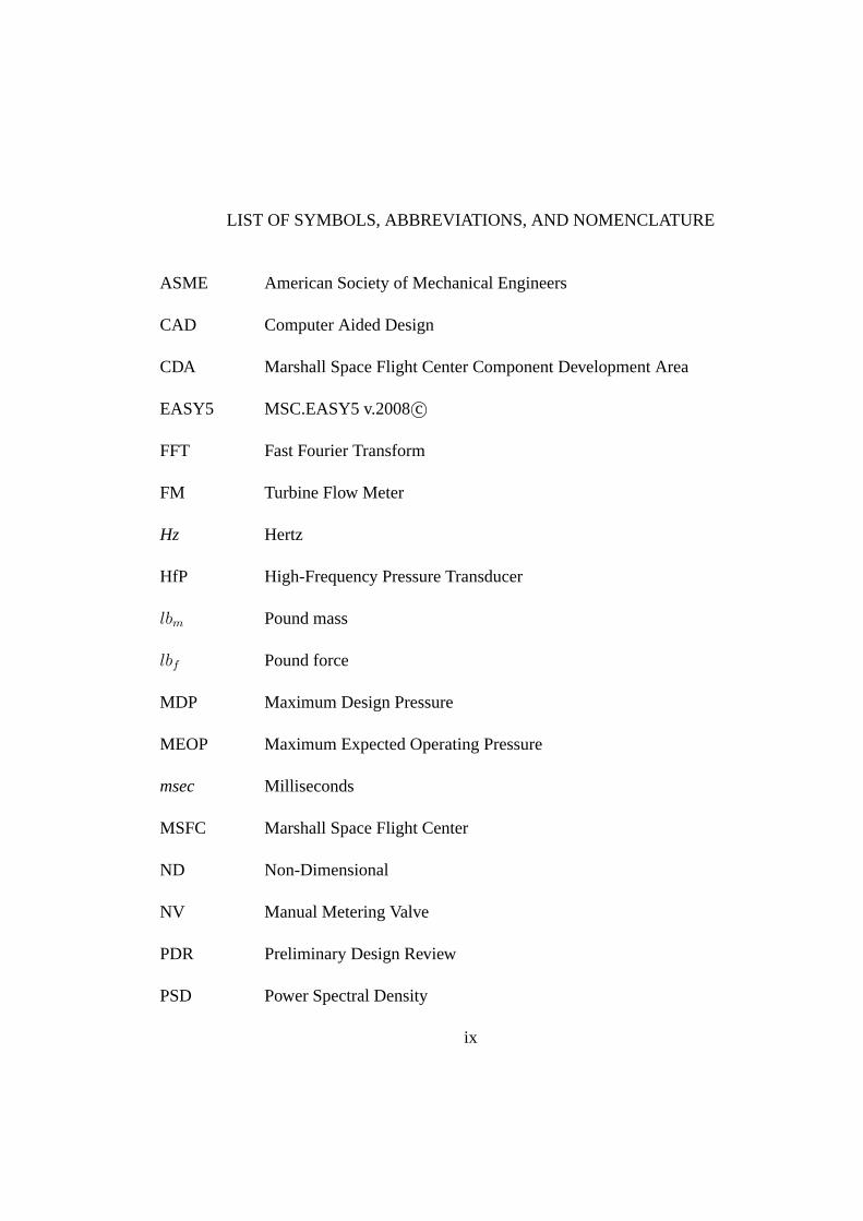
LIST OF SYMBOLS, ABBREVIATIONS, AND NOMENCLATURE
ASME American Society of Mechanical Engineers
CAD Computer Aided Design
CDA Marshall Space Flight Center Component Development Area
EASY5 MSC.EASY5 v.2008c©
FFT Fast Fourier Transform
FM Turbine Flow Meter
Hz Hertz
HfP High-Frequency Pressure Transducer
lbm Pound mass
lbf Pound force
MDP Maximum Design Pressure
MEOP Maximum Expected Operating Pressure
msec Milliseconds
MSFC Marshall Space Flight Center
ND Non-Dimensional
NV Manual Metering Valve
PDR Preliminary Design Review
PSD Power Spectral Density
ix
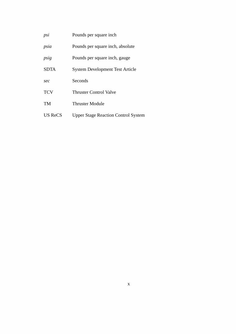
psi Pounds per square inch
psia Pounds per square inch, absolute
psig Pounds per square inch, gauge
SDTA System Development Test Article
sec Seconds
TCV Thruster Control Valve
TM Thruster Module
US ReCS Upper Stage Reaction Control System
x

CHAPTER 1
INTRODUCTION
1.1 Background
The development of the Ares I launch vehicle is an essential step toward completion
of NASA’s Constellation Program. This vehicle will facilitate a new generation of space
access to the International Space Station, the moon, and other destinations within the solar
system. Ares I is a two-stage launch vehicle consisting of a solid First Stage, a bipropel-
lant Upper Stage, the Orion crew capsule and service module [2, 3]. The Upper Stage
utilizes a single J-2X Main Engine fueled by a combination ofliquid oxygen and liquid
hydrogen. During Upper Stage operation, the Upper Stage Reaction Control System (US
ReCS) will provide roll control capability during J2-X operation and three-axis attitude
control capability (roll, pitch, and yaw) after Main EngineCut-Off.
The US ReCS design utilizes a distributed, blow-down, monopropellant hydrazine sys-
tem capable of rapid pulsing at the 100 lbf class. Past NASA launch vehicles such as the
Saturn V [4] and the Space Transportation System (STS) [5] have employed localized,
bipropellant systems for reaction control. The Delta IV [6]and Mars Polar Lander [7],
developed by United Launch Alliance and Jet Propulsion Laboratory respectively, use at-
titude control systems similar to that of the US ReCS with the exception that they are
pressure-regulated systems operated at lower thrust levels than the US ReCS. Therefore,
1

the combination of a distributed blow-down system with higher thrust levels makes the
US ReCS, and all associated testing and analysis, relatively unique within the spacecraft
propulsion community.
Additionally, the methods used at MSFC for transient fluid-flow analysis on the US
ReCS vary from those documented in the literature for similar systems. Based on the
literature review, the Method of Characteristics has provento be the industry standard
with regards to these analyses; however, the work done at MSFC for the US ReCS uses
a Lumped Parameter Method. Past experience using both methods to model the same
system has shown that both provide comparable results, withthe exception being that the
Lumped Parameter Method, with respect to its application inthe modeling software, also
allows for consideration of cavitation in the fluid which is not accounted for in the Method
of Characteristics. In systems like the US ReCS, introduction of additional gas into the
system through cavitation or other means can have a significant impact on the system
dynamics and is thus important to characterize.
To date the analysis of these transient fluid-flows and their effects, specifically water-
hammer, on spacecraft propulsion systems similar to the US ReCS have not been widely
documented. Most available data for similar systems involve waterhammer due to priming
the fluid system and not due to thruster valve closing. Additionally, data for waterham-
mer in response to thruster valve closing exists only for smaller and less complex systems
[7, 8, 9, 10, 11, 12, 13]. Waterhammer is defined as a rise in static pressure inside a
closed system resulting from a sudden deceleration of a fluidsuch as that caused by a
valve closing. Viscous forces and tubing compliance tend todamp out the surge quickly,
2

with the peak pressure lasting only a few milliseconds. The resulting pressure surge due
to valve closure can be more than twice the normal system operating pressure and can in
itself cause significant damage to system tubing and hardware if not properly accounted
for in the design. Additional concerns also arise if there isany residual gas remaining in
the system. During the few milliseconds in which these events occur, a localized pres-
sure increase can result in extreme heating of the gas due to anear-adiabatic compression.
Given the right conditions, these high temperatures can result in an adiabatic compression
detonation of the hydrazine at that location, which can leadto a catastrophic system fail-
ure. Due to these possible failure modes, requirements havebeen imposed upon the US
ReCS design that the Maximum Design Pressure (MDP) of the system encompasses all
transient surge pressure events. Therefore, it is important to sufficiently characterize US
ReCS performance during different mission scenarios in orderto provide a more robust
design.
To accommadate this design process, development tests wereconducted at MSFC in
the fall of 2009 using a water-flow test article for the US ReCS inpreparation for the
Critical Design Review of the flight hardware. A variety of tests covering a range of
supply pressures and duty cycles were conducted to examine system responses for differ-
ent mission scenarios. Numerical models of the test articlefeed system were developed
in conjunction with the development testing for post-test data correlation. The primary
objective of these models was to accurately predict the initial surge pressure after valve
closure, while secondary objectives included the prediction of other aspects of the system
such as frequency and pressure response.
3

Flight System
Analytical
Models
Test Article
Analytical
Model
US ReCS
Test Article
Design
Test Facility
Capabilities
& Limitations
Test Matrix
Development
Pre-Test
Predictions
Flight
System
Predictions
TestingData Review
& Analysis
Model/Data
Correlation
US ReCS
Flight System
Design
Figure 1.1
Flowchart for Design, Test, and Analysis Data and Information Flow
Figure 1.1 shows a general flowchart representation of the information and data flow
through the system design, test, and analysis process. The chart shows how the flight sys-
tem design provided input to both the numerical models and the development test article.
The models of the flight system provided a foundation for the models of the test article.
Pre-test predictions from these models along with the capabilities and limitations of both
the test facility and test article were then used to develop the matrix of tests that were
conducted. Tests were completed, and the resultant data wasreviewed and analyzed. In
addition, the data was used to correlate the numerical models of the test article such that
they provided accurate predictions of the test article performance. From that point, the
updates made to the models of the test article were flowed backup to the flight system
models to provide a more accurate analytical representation of the flight system design.
4
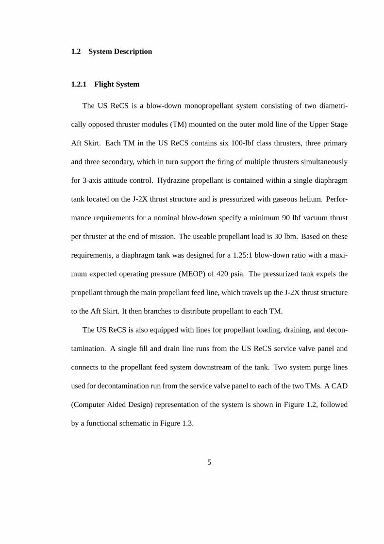
1.2 System Description
1.2.1 Flight System
The US ReCS is a blow-down monopropellant system consisting oftwo diametri-
cally opposed thruster modules (TM) mounted on the outer mold line of the Upper Stage
Aft Skirt. Each TM in the US ReCS contains six 100-lbf class thrusters, three primary
and three secondary, which in turn support the firing of multiple thrusters simultaneously
for 3-axis attitude control. Hydrazine propellant is contained within a single diaphragm
tank located on the J-2X thrust structure and is pressurizedwith gaseous helium. Perfor-
mance requirements for a nominal blow-down specify a minimum 90 lbf vacuum thrust
per thruster at the end of mission. The useable propellant load is 30 lbm. Based on these
requirements, a diaphragm tank was designed for a 1.25:1 blow-down ratio with a maxi-
mum expected operating pressure (MEOP) of 420 psia. The pressurized tank expels the
propellant through the main propellant feed line, which travels up the J-2X thrust structure
to the Aft Skirt. It then branches to distribute propellant to each TM.
The US ReCS is also equipped with lines for propellant loading,draining, and decon-
tamination. A single fill and drain line runs from the US ReCS service valve panel and
connects to the propellant feed system downstream of the tank. Two system purge lines
used for decontamination run from the service valve panel toeach of the two TMs. A CAD
(Computer Aided Design) representation of the system is shown in Figure 1.2, followed
by a functional schematic in Figure 1.3.
5
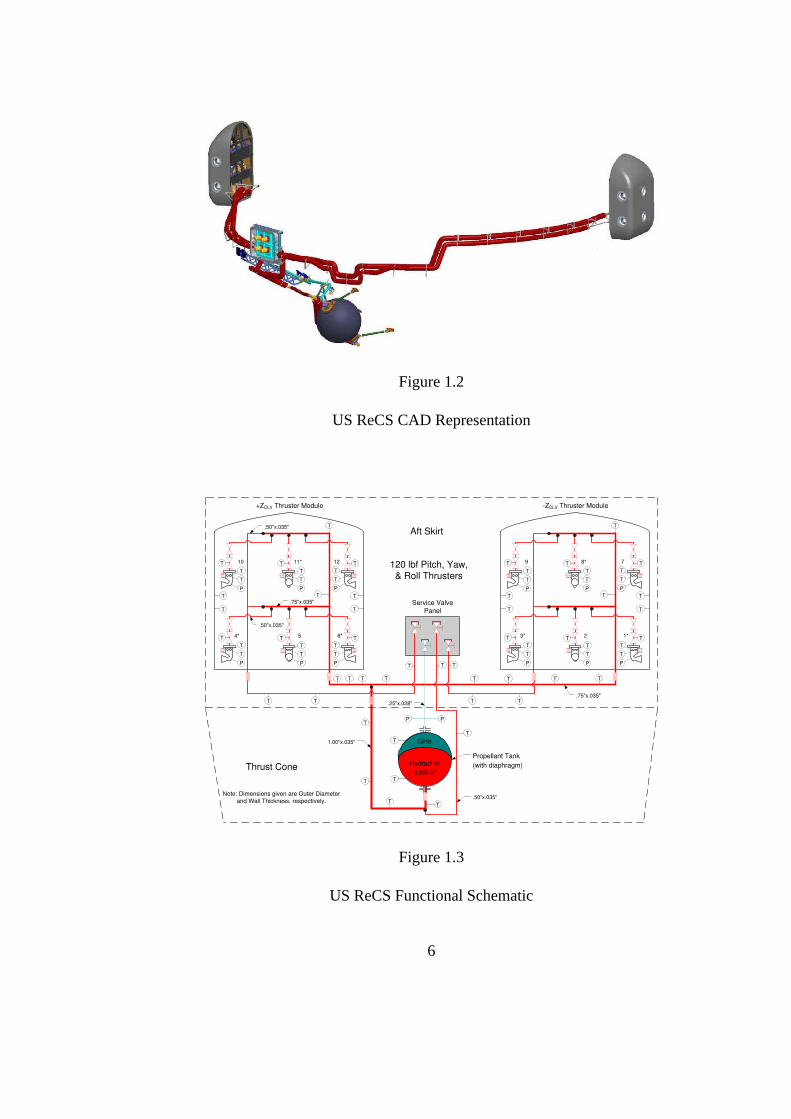
Figure 1.2
US ReCS CAD Representation
+ZCLV Thruster Module
120 lbf Pitch, Yaw,
& Roll Thrusters
T
T
T
T
Service Valve Panel
T
T T
Hydrazine
GHeT
T
PP
Thrust Cone
Aft Skirt
P
T
T
P
T
T
P
T
T
P
T
T
P
T
T
P
T
T
T
T
Note: Dimensions given are Outer Diameter
and Wall Thickness, respectively..50"x.035"
1.00"x.035"
.25"x.028"
.75"x.035"
Propellant Tank
(with diaphragm)5,555 in3
TT
TT
T T TTT T T
TT T
T
1211*10
6*54*
T
T
T
T
T
TTT
-ZCLV Thruster Module
T
T
T
T
T T
P
T
T
P
T
T
P
T
T
P
T
T
P
T
T
P
T
T
T
T
TT
TT
78*9
1*23*
.50"x.035"
.75"x.035"
.50"x.035"
Figure 1.3
US ReCS Functional Schematic
6

1.2.2 System Development Test Article
1.2.2.1 Test Article Overview
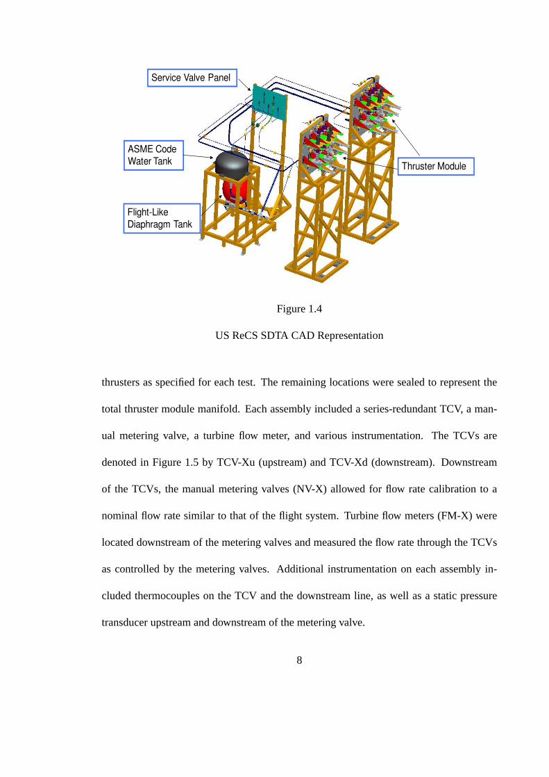
The US ReCS System Development Test Article (SDTA) was a flight-representative
simulator for the US ReCS flight system for Design Analysis Cycle3A-S-RevA [14]. It
was tested at the MSFC CDA to evaluate integrated system levelperformance charac-
teristics and verify analytical models as part of the critical design activities. The SDTA
used a single flight-similar diaphragm tank mounted in approximately the same relative
location and orientation as the flight tank. An ASME (American Society of Mechanical
Engineers) code tank was also incorporated into the test article for waterhammer testing
to avoid excessive pressure cycling of the diaphragm tank and to test over a range of spec-
ified regulated pressures. A propellant distribution manifold representative of the flight
configuration was fabricated with instrumentation ports for pressure transducers. Welded
assemblies were used when possible to provide similarity tothe flight propellant mani-
fold, with exceptions at flex hose fitting connections, inlets to the Thruster Control Valve
(TCV) assemblies, and break-point locations used to facilitate transportation. All SDTA
components were mounted on a test fixture designed to decouple feed system dynamics,
as shown in Figure 1.4. SDTA components were mounted to the test fixture using a similar
approach to flight bracketing such that the dynamic responseof the tubing was simulated.
Four TCV assemblies were fabricated for installation at fourof the twelve possible
locations within the thruster modules (L1 through L12 in Figure 1.5). These assemblies
were capable of being moved between thruster valve locations depending on the required
7
Service Valve Panel
Thruster Module
ASME Code
Water Tank
Flight-Like
Diaphragm Tank
Figure 1.4
US ReCS SDTA CAD Representation
thrusters as specified for each test. The remaining locations were sealed to represent the
total thruster module manifold. Each assembly included a series-redundant TCV, a man-
ual metering valve, a turbine flow meter, and various instrumentation. The TCVs are
denoted in Figure 1.5 by TCV-Xu (upstream) and TCV-Xd (downstream). Downstream
of the TCVs, the manual metering valves (NV-X) allowed for flowrate calibration to a
nominal flow rate similar to that of the flight system. Turbineflow meters (FM-X) were
located downstream of the metering valves and measured the flow rate through the TCVs
as controlled by the metering valves. Additional instrumentation on each assembly in-
cluded thermocouples on the TCV and the downstream line, as well as a static pressure
transducer upstream and downstream of the metering valve.
8

Figure 1.5
US ReCS SDTA Functional Schematic
9

1.2.2.2 System Instrumentation
Other system instrumentation included ten dynamic pressure transducers (HfP-XXX),
one at the end of each purge line on the service valve panel and, due to data-system chan-
nel availability, one each at eight of the twelve TCV locations in the thruster modules. A
breakdown of the system instrumentation by type is shown in Table 1.1 and is comparable
to the instrumentation described in the literature for similar tests [10, 9, 7]. Dynamic pres-
sure transducers and static pressure transducers were co-located in the same instrumenta-
tion block. Other static pressure measurements (P-XXX) were taken at various locations
throughout the system and are shown in Figure 1.5. The pressurization system for both
the diaphragm tank and the ASME code tank also contained multiple static pressure and
temperature measurements. Other instrumentation included biaxial strain gauges at four
of the twelve TCV locations to measure the effects of waterhammer on tubing, as well as
accelerometers on TCVs A and B to provide data during valve actuation.
10

Table 1.1
System Instrumentation
Type Quantity RangeData Rate
(kHz)
Pressure Transducers - Static 33 0 to 2000 psig10
1
12
Pressure Transducers - Dynamic 10 0 to 1000 to 5000 psid 50
Thermocouples 27 0 to 160°F 0.1
Accelerometers 2 0 to 25 g 50
Strain Guages 10Axial and Hoop 0 - 70
strain50
Flow Meters 4
FM-A: 2.0 - 12.4 GPM;
FM-B, FM-C, FM-D:
0.6 - 5.0 GPM
1
1 For those adjacent to a dynamic transducer
2 Stand alone transducer
11
CHAPTER 2
MODELING AND ANALYSIS
2.1 Modeling in the Time Domain
Waterhammer can be modeled using many different methods, such as Finite Element
Analysis [15], Method of Characteristics [7, 16, 17, 18, 19, 20, 21, 22, 23, 24, 25, 26],
and Impedance Analysis [8, 22]. Another method for modelingwaterhammer effects is
the Lumped Parameter Method, which is employed by the EASY5 analysis package used
at MSFC. MSCSoftware.EASY5 v.2008c© is a commercially available, dynamic system
modeling package with a heritage for modeling spacecraft propulsion systems. EASY5
is capable of modeling transient pressure wave phenomena, such as waterhammer, us-
ing transient forms of mass and energy conservation. The Thermal Hydraulic Library of
EASY5 is a collection of fluid components (pipes, valves, orifices, etc.) whose input pa-
rameters and output variables are connected to other components to form complex fluid
systems. EASY5 provides a robust modeling framework for waterhammer model devel-
opment and was used to simulate various systems on Ares I. TheEASY5 waterhammer
model of the US ReCS SDTA, shown in Figure 2.1, was initially based on an existing US
ReCS flight system model. However, throughout the SDTA data review and model corre-
lation process, many updates and changes were made to reflectthe differences between the
12
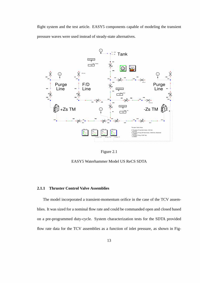
flight system and the test article. EASY5 components capableof modeling the transient
pressure waves were used instead of steady-state alternatives.
Bulk Modulus
TCV - B
.93
TCV - A
HydraulicFluid
14
Bulk Modulus
.694
P = 392
T = 95
VAL_PA
PSV-02
TCV - CTCV - D
.194
VAL_PA45
Bulk Modulus
MV-01
VAL_PA21
S_Out_T13
ROV-05
S_Out_T12 S_Out_T1
-Zs TM+Zs TM
Purge Line
Purge Line
F/DLine
Thruster Valve Area:
2 Thrusters Firing Nominally, 0.52 lb/s- 0.00793"2 Thrusters Firing Off-Nominally, 0.563 lb/s (Stacked)- 0.00865"1 Thruster Firing, 0.567 lb/s- 0.00865"
Tank
Figure 2.1
EASY5 Waterhammer Model US ReCS SDTA
2.1.1 Thruster Control Valve Assemblies
The model incorporated a transient-momentum orifice in the case of the TCV assem-
blies. It was sized for a nominal flow rate and could be commanded open and closed based
on a pre-programmed duty-cycle. System characterization tests for the SDTA provided
flow rate data for the TCV assemblies as a function of inlet pressure, as shown in Fig-
13

ure 2.2. The flow rate data for all TCV assemblies was combined and averaged, converted
to a discharge coefficient as a function of inlet pressure, and then incorporated into the
modeled TCV assemblies. Flow meter data measured downstreamof the TCVs were also
used to estimate a valve closing time. Likewise, high-frequency pressure data measured
upstream of the TCVs were used to establish a closing profile for the valves, shown in
Table 2.1, and represented the flow cross-sectional area as afunction of time. Initially, this
profile was assumed to be a linear closing over 0.5 msec, but upon inspection of the data
a more parabolic closing profile over 0.4 msec was implemented in the model to better
represent the data.
Inle
t P
ress
ure
[psi
g]/F
low
Rat
e [g
pm
]
2 3 4 5 6
16
14
12
10
8
6
4
2
700
600
500
400
300
200
Time (sec)
FM-A P403
Figure 2.2
Typical Pressure and Flow Rate Response
14

Table 2.1
TCV Closing Profile
Time (msec) Position * Flow Area (in2)
0 1 7.93 x 10⁻³
0.3 0.75 5.95 x 10⁻³
0.4 0 0.0
* (0=Closed, 1=Open)
2.1.2 System Tubing
Transient momentum pipe components were used for all the system tubing, from the
tank outlet to the thruster valve inlets. The appropriate lengths and inner diameters were
input into each component, along with the number of nodes foreach pipe section. An in-
crease in the number of nodes in each pipe section results in increased computational time
for the model; therefore, an iterative process was used to determine the minimum num-
ber of nodes required to sufficiently characterize the waterhammer pressure wave for each
pipe. The bulk modulus of the tubing material was input to produce more accurate speed
of sound calculations within each pipe component. Pressuredrops throughout the propel-
lant feed system were initially based on analytical relations and flight system conditions
but were updated to reflect the SDTA test data by modifying thesurface roughness of each
pipe component. A value for the tubing surface roughness wasinput based on published
information for stainless steel tubing. An input in each pipe component for a frequency-
dependent friction multiplier was also utilized to help dampen the pressure oscillations.
15

While relative height changes in tubing runs were included inthe model, the contribu-
tion of tube bends to the pressure drop was considered negligible and was therefore not
included in the model.
2.1.3 ASME Code Tank
The ASME code tank used for waterhammer testing was not specifically modeled in
EASY5, but was represented as a boundary condition at a predefined pressure. This deci-
sion was justified based upon three reasons. First, the addition of the ASME code tank to
the model would increase the complexity of the model and provide a significant negative
impact on the run-time for each simulation. Second, only fivemilliseconds of steady-state
flow were simulated prior to the valve closing, so the water-volume change in the tank was
considered to be negligible. Third, with regards to the waterhammer event, neglecting to
model the tank will ensure less overall system damping to thepressure wave and thus a
more conservative result.
2.1.4 Entrained Gas
The capability to input the void fraction of entrained gas ina fluid also exists in EASY5
and affects the calculation of the fluid speed of sound and thesystem damping. The term
void fraction refers to the ratio of the total volume of undissolved gas present at steady-
state conditions to the total volume of the system, including both liquid and gas volume.
This value is highly dependent on the initial conditions of the system prior to liquid filling
and is one of the primary drivers behind vacuum-filling liquid propulsion systems similar
16
to the US ReCS. As more gas is introduced into the system, it decreases the bulk speed of
sound of the fluid-gas mixture and increases the overall system damping. The void fraction
of entrained gas was determined using the system geometry and the pre-water-load pad
pressure. It was then possible to determine, assuming an isothermal compression, the final
volume of displaced gas that would eventually be trapped by the liquid fill. The model
assumed a homogenous mixture of gas and liquid, though realistically the bulk of the gas
was trapped in various locations throughout the system. However, since it was impossible
to determine with absolute certainty the location of those gas pockets, this assumption was
the best that could be made.
2.2 Analysis in the Frequency Domain
Frequency analysis is a useful method for data analysis, especially with regard to de-
termining the natural frequency and frequency matching in complex fluid systems such
as the US ReCS SDTA. The Fast Fourier Transform (FFT) was employed to convert both
experimental and simulation data into the frequency domainfor analysis utilizing Power
Spectral Density (PSD) curves [7]. MATLAB was used to perform FFTs to convert both
experimental and simulation data into Power Spectral Density (PSD) curves to aid in data
analysis and comparison. Straight-tube harmonics were also employed to provide a simple
and quick way of estimating major system frequencies. Comparing these results to PSD
curves of the test data and simulation results provided a secondary means for troubleshoot-
ing during the model correlation process in order to ensure that the major frequencies
exhibited by the test article were captured by the fluid model.
17
2.3 Statistical Analysis
In addition to examining the data in both the time and frequency domain, statistical
analyses were also employed to provide further comparisonsbetween the test data and
simulation results. Percent error for each individual pressure measurement were compared
between tests, and average percent errors for entire tests were used as one of many metrics
for establishing satisfactory agreement between the testsand simulations. Generally, the
lower the average percent error the better with regards to these model correlations. Another
tool utilized was standard deviations, which allowed the examination of the variation in
measured pressure over multiple runs of a single test series. These values provided another
means for troubleshooting during the model correlation process. Low standard deviations
were indicative of consistent and repeatable pressure measurements, while high values
suggested inconsistencies in the system between tests or possibly even instrumentation
error.
18
CHAPTER 3
RESULTS AND DISCUSSION
3.1 Experimental
Eighty-two tests specific to waterhammer were conducted during testing of the US
ReCS SDTA using an array of supply pressures, TCV sequences, TCV configurations,
and overall system configurations. Most TCV sequences were run at a low (315 psia),
nominal (385 psia), or high supply pressure (410 psia) in reference to the flight system
MEOP of 420 psia. Testing was performed in three different system configurations. The
first configuration is represented schematically in Figure 1.5. TCVs A, B and C were
located at L3, L2, and L1, respectively, in the -Zs Thruster Module (TM) with TCV-D
being located at L6 in the +Zs TM. The second configuration required repositioning of
two TCVs such that each TM was configured with a primary and redundant roll TCV.
TCVs A and B were relocated to L7 and L12 respectively, while TCVs C and D remained
in the same locations (L1 and L6, respectively). The third configuration was the same as
the second configuration with the exception that the purge lines were removed. The surge
pressures measured at the service valves in the purge lines met or exceeded those measured
in the TMs during many of the previous tests; therefore, a third configuration was tested.
Out of the eighty-two total waterhammer tests, a set of twelve nominal baseline tests
were conducted using the first configuration to provide data points to demonstrate system
19
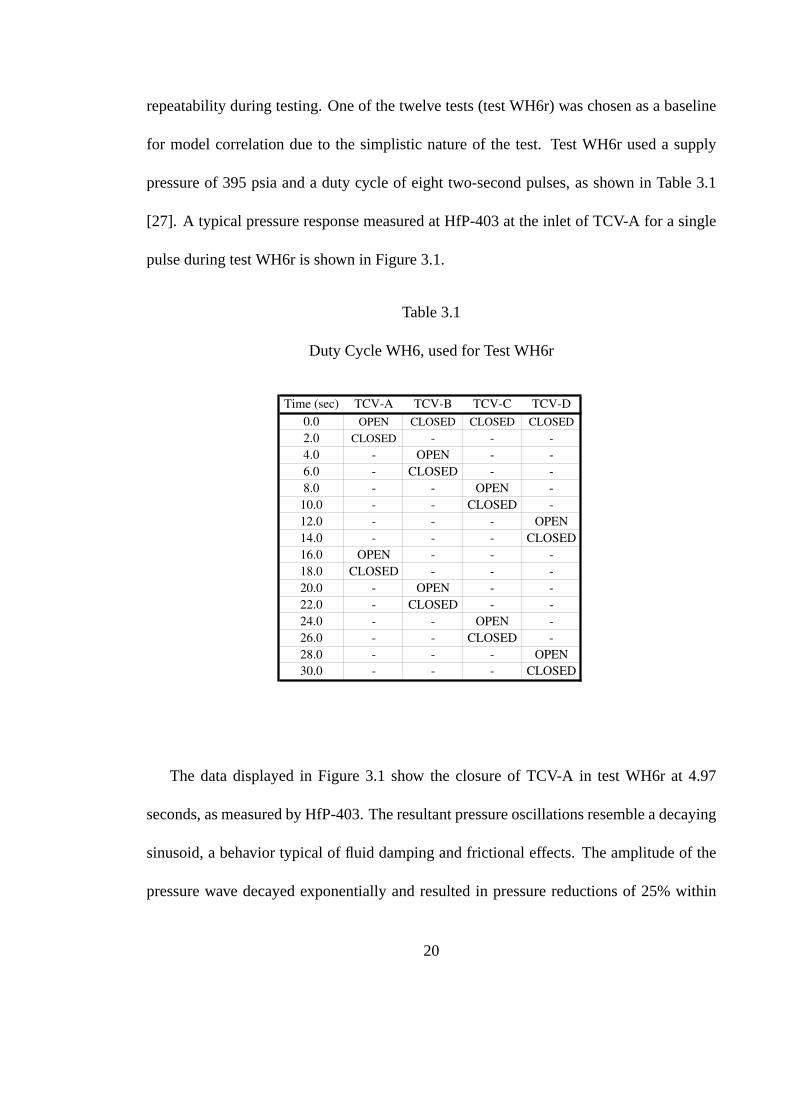
repeatability during testing. One of the twelve tests (testWH6r) was chosen as a baseline
for model correlation due to the simplistic nature of the test. Test WH6r used a supply
pressure of 395 psia and a duty cycle of eight two-second pulses, as shown in Table 3.1
[27]. A typical pressure response measured at HfP-403 at theinlet of TCV-A for a single
pulse during test WH6r is shown in Figure 3.1.
Table 3.1
Duty Cycle WH6, used for Test WH6r
Time (sec) TCV-A TCV-B TCV-C TCV-D
0.0 OPEN CLOSED CLOSED CLOSED
2.0 CLOSED - - -
4.0 - OPEN - -
6.0 - CLOSED - -
8.0 - - OPEN -
10.0 - - CLOSED -
12.0 - - - OPEN
14.0 - - - CLOSED
16.0 OPEN - - -
18.0 CLOSED - - -
20.0 - OPEN - -
22.0 - CLOSED - -
24.0 - - OPEN -
26.0 - - CLOSED -
28.0 - - - OPEN
30.0 - - - CLOSED
The data displayed in Figure 3.1 show the closure of TCV-A in test WH6r at 4.97
seconds, as measured by HfP-403. The resultant pressure oscillations resemble a decaying
sinusoid, a behavior typical of fluid damping and frictionaleffects. The amplitude of the
pressure wave decayed exponentially and resulted in pressure reductions of 25% within
20
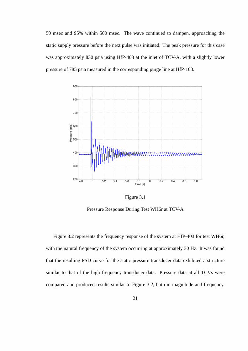
50 msec and 95% within 500 msec. The wave continued to dampen,approaching the
static supply pressure before the next pulse was initiated.The peak pressure for this case
was approximately 830 psia using HfP-403 at the inlet of TCV-A, with a slightly lower
pressure of 785 psia measured in the corresponding purge line at HfP-103.
4.8 5 5.2 5.4 5.6 5.8 6 6.2 6.4 6.6 6.8200
300
400
500
600
700
800
900
Pre
ssure
[psia
]
Time [s]
Figure 3.1
Pressure Response During Test WH6r at TCV-A
Figure 3.2 represents the frequency response of the system at HfP-403 for test WH6r,
with the natural frequency of the system occurring at approximately 30 Hz. It was found
that the resulting PSD curve for the static pressure transducer data exhibited a structure
similar to that of the high frequency transducer data. Pressure data at all TCVs were
compared and produced results similar to Figure 3.2, both inmagnitude and frequency.
21

This suggests the frequency spectrum of the pressure data within the TMs are equivalent,
irrespective of pressure transducer location. The pressure data at the TCV locations were
then compared to that recorded at the purge valves. The PSD curve at each purge valve
also produced a similar spectrum to that present in the TMs.
101
102
103
0
5
10
15
20
25
Spectr
al P
ow
er
[dB
]
Frequency [Hz]
Natural Frequency
Figure 3.2
Frequency Domain Representation of Experimental SDTA Data
3.2 Analytical vs. Experimental
Simulations for the US ReCS SDTA EASY5 model were run using the methodology
laid out in the previous chapter. The appropriate values forsystem dimensions were input,
along with friction parameters and a gas-liquid void fraction. Pre-test predictions showed
good correlations for maximum surge pressure to within 15% of the test data. The flow
22
rates and pressure drops through the system also matched well with the test data. How-
ever, other aspects of the model results, such as the dampingand frequency of the pressure
response, exhibited significant differences. The simulation results were underdamped and
displayed a higher natural frequency (approximately 45 Hz)than that of test data, though
the natural frequency did change slightly from test to test.This change in frequency be-
tween tests could be attributed to varying amounts of water in the ASME code tank, as
well as the amount and location of trapped gas in the system.
Modifications were made to the model in several areas in an attempt to correct these
discrepancies. The number of nodes in each pipe segment was examined and, in most
cases, increased in order to refine each segments ability to capture the amplitude of the
pressure wave. A range of values for both the frequency dependent friction multiplier and
the gas-liquid void fraction were examined to determine their effects on both frequency
and damping. FFTs of both the test data and simulation results were also employed in an
attempt to identify the source of the frequency differences. The high-frequency pressure
measurement (HfP-403) at the inlet of TCV-A for the first pulseof test WH6r was used
during these modifications for model calibration.
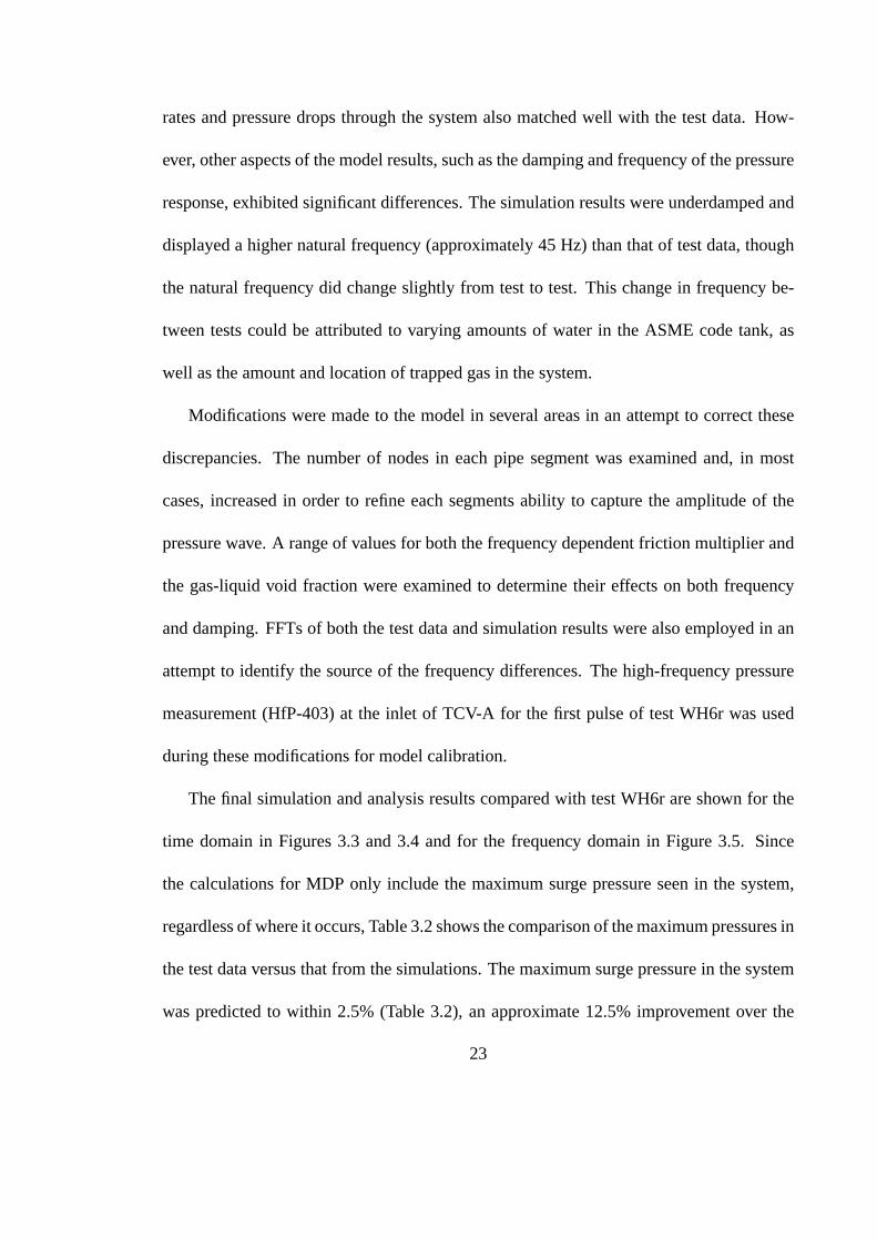
The final simulation and analysis results compared with testWH6r are shown for the
time domain in Figures 3.3 and 3.4 and for the frequency domain in Figure 3.5. Since
the calculations for MDP only include the maximum surge pressure seen in the system,
regardless of where it occurs, Table 3.2 shows the comparison of the maximum pressures in
the test data versus that from the simulations. The maximum surge pressure in the system
was predicted to within 2.5% (Table 3.2), an approximate 12.5% improvement over the
23

pre-test predictions. It should be noted that the EASY5 model predicts the maximum
surge pressure to occur at HfP-103 in the -Zs TM purge line, whereas the test data shows
the maximum occurring at HfP-403 in the -Zs TM at the inlet to TCV-A. For HfP-403,
the model predicts the surge pressure to within 2.0%.The average percentage error for all
high frequency pressure measurements throughout the system for the initial surge pressure
peak was 5.21%.
4.8 5 5.2 5.4 5.6 5.8 6 6.2 6.4 6.6 6.8200
300
400
500
600
700
800
900
Pre
ssure
[psia
]
Time [s]
Simulation
Experimental
~30 Hz
Figure 3.3
Test vs. Simulation: Full Simulation
The model also predicts the natural frequency of the system around 30 Hz, along with
other notable frequencies found in the test data at approximately 40 Hz and in the 700-800
Hz range. The 40 Hz frequency is thought to correspond to the propagation of pressure
24
4.95 5 5.05 5.1 5.15 5.2100
200
300
400
500
600
700
800
900
1000
Pre
ssure
[psia
]
Time [s]
Simulation
Experimental
Figure 3.4
Test vs. Simulation: TCV closure and the first few pressure oscillations
101
102
103
0
5
10
15
20
25
Spectr
al P
ow
er
[dB
]
Frequency [Hz]
Simulation
Experimental
Figure 3.5
Test vs. Simulation: PSD Curves for HfP-403 at TCV-A
25

Table 3.2
Percent Error Between Test Data and Model Predictions
Table 3 – Percent Error Between Test Data and Model Predictions
Test Model % Error Test Model % Error Test Model % Error
HfP-101 540 528 2.22% 531 528 0.56% 518 525 1.35%
HfP-103 623 683 9.63% 621 683 9.98% 622 679 9.16%
HfP-304 429 435 1.40% 428 435 1.64% 419 433 3.34%
HfP-306 439 427 2.73% 434 427 1.61% 423 425 0.47%
HfP-310 345 427 23.77% 361 427 18.28% 416 424 1.92%
HfP-312 362 427 17.96% 382 427 11.78% 411 424 3.16%
HfP-401 571 506 11.38% 553 506 8.50% 542 503 7.20%
HfP-402 542 529 2.40% 540 529 2.04% 560 526 6.07%
HfP-403 676 678 0.30% 640 678 5.94% 687 674 1.89%
HfP-407 520 567 9.04% 500 567 13.40% 477 564 18.24%
Maximum Pressure 676 683 1.04% 640 683 6.72% 687 679 1.16%
Average Percent Error 8.08% 7.37% 5.28%
Test Model % Error Test Model % Error Test Model % Error
HfP-101 640 638 0.31% 646 643 0.46% 632 627 0.79%
HfP-103 746 766 2.68% 744 773 3.90% 757 802 5.94%
HfP-304 515 529 2.72% 519 534 2.89% 509 521 2.36%
HfP-306 521 525 0.77% 528 530 0.38% 517 512 0.97%
HfP-310 420 526 25.24% 446 531 19.06% 506 511 0.99%
HfP-312 437 522 19.45% 469 527 12.37% 503 512 1.79%
HfP-401 662 636 3.93% 692 642 7.23% 675 601 10.96%
HfP-402 637 627 1.57% 660 633 4.09% 656 629 4.12%
HfP-403 776 801 3.22% 827 808 2.30% 813 798 1.85%
HfP-407 614 644 4.89% 628 650 3.50% 607 672 10.71%
Maximum Pressure 776 801 3.22% 827 808 2.30% 813 802 1.35%
Average Percent Error 6.48% 5.62% 4.05%
Test Model % Error Test Model % Error Test Model % Error
HfP-101 675 663 1.78% 671 661 1.49% 658 666 1.22%
HfP-103 828 847 2.29% 784 843 7.53% 784 850 8.42%
HfP-304 547 553 1.10% 540 550 1.85% 533 555 4.13%
HfP-306 552 543 1.63% 548 541 1.28% 540 546 1.11%
HfP-310 448 543 21.21% 465 540 16.13% 524 545 4.01%
HfP-312 466 543 16.52% 489 541 10.63% 521 546 4.80%
HfP-401 719 637 11.40% 721 634 12.07% 727 640 11.97%
HfP-402 700 666 4.86% 684 663 3.07% 688 669 2.76%
HfP-403 834 842 0.96% 857 839 2.10% 831 846 1.81%
HfP-407 655 710 8.40% 655 707 7.94% 637 713 11.93%
Maximum Pressure 834 847 1.56% 857 843 1.63% 831 850 2.29%
Average Percent Error 7.01% 6.41% 5.21%
WH6b WH6c WH6rPressure Measurement*
Pressure Measurement*
Pressure Measurement*WH4b WH4c WH4r
WH5b WH5c WH5r
26

waves between the thruster modules and the tank, while the 700-800 Hz frequencies are
thought to be oscillations within the thruster modules themselves. These notions are based
on calculations performed using simple straight tube harmonics; therefore, a more in-depth
analysis will be required to confirm the source of these frequencies. Comparisons were
also made with eight other tests that employed the same duty cycle as test WH6r. With
exception for the supply pressure, inputs for the EASY5 waterhammer model remained
constant for all eight test cases to provide consistency between the simulations. The ap-
proximate supply pressure was 310 psia for the tests designated with WH4x, 380 psia for
WH5x, and 400 psia for WH6x. The results of these comparisons are tabulated along with
the baseline case, WH6r, in Table 3.2. The results for all ninetests showed the maximum
surge pressures predicted to within 6.72 %, with the averagepercent error for all pressure
measurements to within 8.08%.
3.3 Resolution of Discrepancies and Error
A primary difference between the simulation and experimental data is that the simula-
tion damps out faster than the experimental data (Figure 3.3), resulting in an underpredic-
tion of the amplitude of the natural frequency (Figure 3.5) [28]. This result was consistent
across all the simulations that were run and compared with test data. It is believed this
discrepancy in the magnitude of the natural frequency (i.e.system damping) is due to one
or more characteristics of the US ReCS SDTA (e.g. ASME code tank, fluid/structure inter-
action, frequency-dependent friction, etc.) that are currently unaccounted for or modeled
incorrectly in the EASY5 model. Since accurate prediction of the system damping was not
27
the primary objective of the system modeling and proved to have little to no impact on the
peak surge pressure, the discrepancy was accepted and deferred as future work. Updating
the EASY5 waterhammer model for both the test article and theflight system will focus on
establishing a better correlation between the model and test data with regards to damping
in hopes to get rid of this disparity.
Another error, which can be noted from Table 3.2, is that two of the ten measurements
(HfP-310 and HfP-312) consistently exhibit higher error (greater than 10%) than the other
eight. The most likely explanation for these errors is high variability in those individual
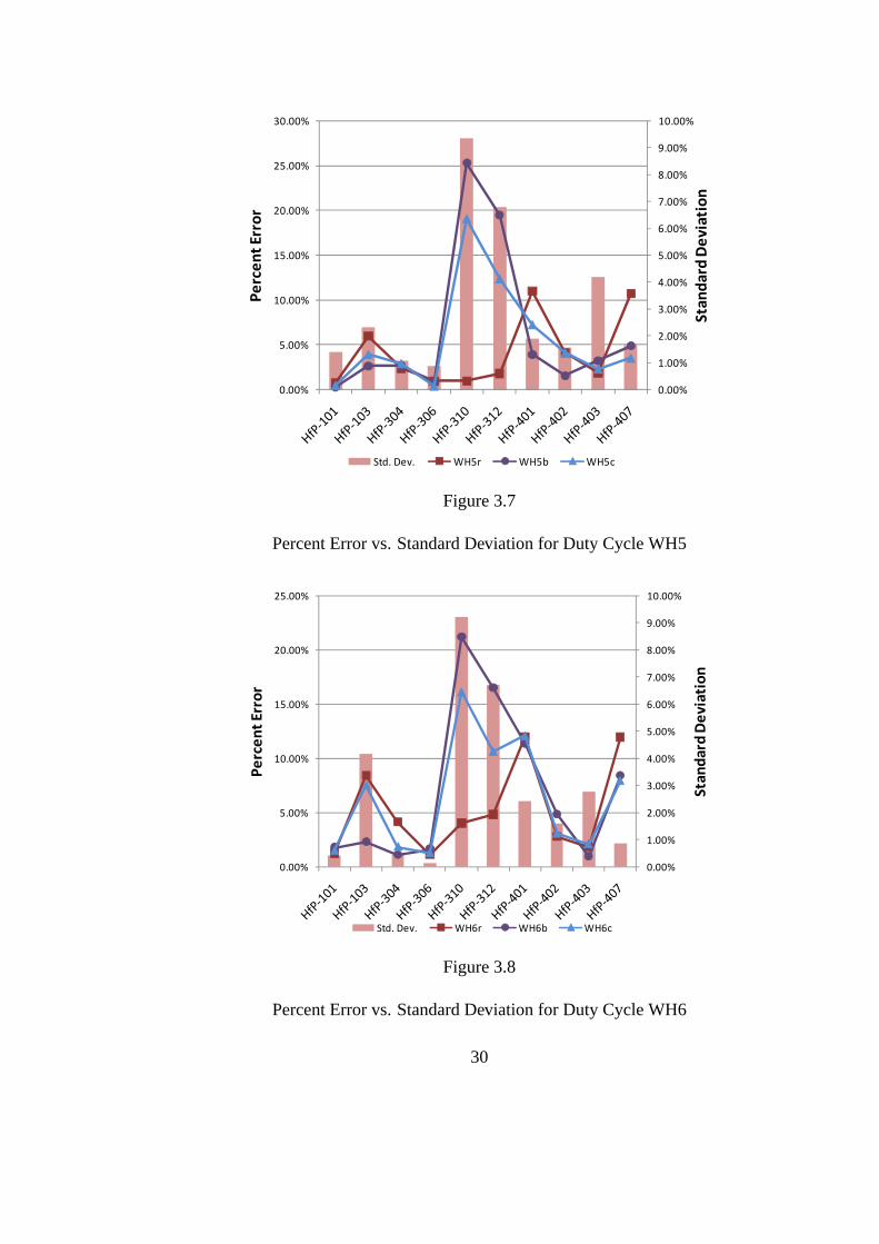
pressure measurements from test to test. Figures 3.6, 3.7, and 3.8 provide a comparison
of the percent error in the predicted pressure measurementsversus the standard deviation
of each pressure measurement. Each figure contains plots of the percent error in predicted
measurements for three separate runs of a single test series(i.e. WH4b, WH4c, WH4r), as
well as a plot of the standard deviation of each pressure measurement across those three
runs. In order to account for different static inlet pressures for the different tests compared,
the pressure measurements (i.e. the peak surge pressure values) were non-dimensionalized
with respect to their reference static inlet pressures.
The results shown in Figures 3.6, 3.7, and 3.8 illustrate a strong correlation between
high percent error and high variability in the pressure measurements. The pressure mea-
surements HfP-310 and HfP-312 consistently showed the highest error across all the tests
examined, and consistently those measurements also had thehighest variability from test
to test. High variability in the pressure measurement couldbe caused by a number of
things. Based on the results shown in Table 3.2, the model over-predicted the pressures at
28

those two locations, which corresponded to locations in thesystem that never experienced
flow. It is likely that during the initial water fill process, residual gas in the system became
trapped at these locations and damped the pressure responsemeasured by the transducer
at those locations. Regardless of the reason for the error, these areas of high variability
ultimately result in parts of the system that are less predictable and more difficult to model.
There is no way to predict from test to test where these areas of high variability will occur,
other than they seem to tend more toward the areas of low or no flow based on the data that
has been examined thus far. For future analyses and simulations, it will have to be decided
on a case by case basis how these are handled to most accurately reflect the system being
modeled.
0.00%
5.00%
10.00%
15.00%
20.00%
25.00%
0.00%
5.00%
10.00%
15.00%
20.00%
25.00%
StandardDeviation
PercentError
Std. Dev. WH4r WH4b WH4c
Figure 3.6
Percent Error vs. Standard Deviation for Duty Cycle WH4
29
0.00%
1.00%
2.00%
3.00%
4.00%
5.00%
6.00%
7.00%
8.00%
9.00%
10.00%
0.00%
5.00%
10.00%
15.00%
20.00%
25.00%
30.00%
StandardDeviation
PercentError
Std. Dev. WH5r WH5b WH5c
Figure 3.7
Percent Error vs. Standard Deviation for Duty Cycle WH5
0.00%
1.00%
2.00%
3.00%
4.00%
5.00%
6.00%
7.00%
8.00%
9.00%
10.00%
0.00%
5.00%
10.00%
15.00%
20.00%
25.00%
StandardDeviation
PercentError
Std. Dev. WH6r WH6b WH6c
Figure 3.8
Percent Error vs. Standard Deviation for Duty Cycle WH6
30

CHAPTER 4
CONCLUSIONS
Waterhammer tests were performed using the US ReCS SDTA to provide anchoring
data for numerical models of the US ReCS flight system. Comparisons of the simulation
results to multiple sets of test data for the SDTA showed strong correlations for both the
pressure and frequency responses of the system. Maximum surge pressures from the test
data were predicted to within 6.75% by the EASY5 model. The natural frequency of the
system was not captured as strongly in the model as it was in the test data as a result
of the overdamping of the waterhammer pressure wave in the simulations. Future work
will focus on improvements to the EASY5 model to provide better correlation with the
system damping. In addition, tests involving multiple TCV closings will be examined
and compared to simulation results. The results presented within this thesis validate the
models ability to predict system performance of the SDTA andprovide confidence that
the maximum surge pressures can be accurately modeled and predicted for the US ReCS
flight system.
31
REFERENCES
[1] J. Williams, K. Holt, and W. Stein, “Testing and Modelingof the Ares I UpperStage Reaction Control System,”Proceedings: 57th JANNAF Propulsion Meeting,Colorado Springs, CO, 2010, JANNAF, JANNAF-1163.
[2] M. Dervan, J. Williams, K. Holt, J. Wiley, A. Sivak, and J.Morris, “NASA Ares I Up-per Stage Reaction Control System Cold Flow Development Test Program Results,”Proceedings: 57th JANNAF Propulsion Meeting, Colorado Springs, CO, 2010, JAN-NAF, JANNAF-1370.
[3] A. Turpin, Upper Stage Reaction Control System (ReCS) Subsystem Design Specifi-cation, Tech. Rep., National Aeronautics and Space Administration, Ares-USO-SE-25718.
[4] Saturn Technical Information Handbook, Tech. Rep., George C. Marshall SpaceFlight Center, May 1966, NASA-TM-109688.
[5] Space Shuttle Orbiter Reaction Control Subsystem Smartbook, Tech. Rep., RockwellInternational, November 1989, Ares-USO-SE-25718.
[6] D. M. Hart, “The Boeing Company EELV/Delta IV Family,”Proceedings: Defenseand Civil Space Programs Conference. AIAA, 1998, AIAA-1998-5166.
[7] T. Martin, L. Rockwell, and C. Parish, “Test and Modeling ofthe Mars 98 LanderDescent Propulsion System Waterhammer,” AIAA, 1998, AIAA-98-3665-858.
[8] A. Malesiska, M. Chorzelski, and M. Mitosek, “Experimental analysis of naturalfrequency of water column due to water hammer in series pipe systems,” Warsaw,2002, ICHSE.
[9] W. H. Hsieh, C. Y. Lin, and A. S. Yang, “Blowdown and Waterhammer Behavior ofMono-propellant Feed Systems for Satellite Attitude and Reaction Control,” AIAA,1997, AIAA-1997-3224-161.
[10] I. Gibek and Y. Maisonneuve, “Waterhammer Tests with Real Propellants,” Pro-ceedings: 41st Joint Propulsion Conference. AIAA, 2005, AIAA-2005-4081.
[11] R. Lecourt and J. Steelant, “Experimental Investigation of Waterhammer in Simpli-fied Basic Pipes of Satellite Propulsion Systems,”Journal of Propulsion and Power,vol. 23, no. 6, November-December 2007, pp. 1214–1224.
32

[12] R. P. Prickett, E. Mayer, and J. Hermel, “Water Hammer in aSpacecraft PropellantFeed System,”Journal of Propulsion and Power, vol. 8, no. 3, May-June 1992, pp.592–597.
[13] J. Molinsky, “Water Hammer Test of the SeaStar Hydrazine Propulsion System,”Proceedings: 33rd Joint Propulsion Conference. AIAA, 1997, AIAA-97-3226.
[14] M. Dervan, US ReCS System Level Cold Flow Development Test Plan, Tech. Rep.,National Aeronautics and Space Administration, RCS-PLAN-DTP-030.
[15] R. Leishar, “Dynamic Pipe Stresses During Waterhammer:A Finite Element Ap-proach,”ASME Journal of Pressure Vessel Technology, vol. 129, May 2007.
[16] E. Wylie, Resonance in Pressurized Piping Systems, doctoral dissertation, The Uni-versity of Michigan, November 1964.
[17] W. Zielke, Frequency Dependent Friction in Transient Pipe Flow, doctoral disserta-tion, The University of Michigan, December 1966.
[18] E. Wylie and W. Zielke,Propellant Line Dynamics, Final report, The University ofMichigan, September 1967.
[19] D. M. Contractor, The Effect of Minor Losses on Waterhammer Pressure Waves,doctoral dissertation, The University of Michigan, December 1963.
[20] C. Lai, A Study of Waterhammer Including Effect of Hydraulic Losses, doctoraldissertation, The University of Michigan, December 1961.
[21] W. Yow, Analysis and Control of Transient Flow in Natural Gas Piping Systems,doctoral dissertation, The University of Michigan, 1971.
[22] V. L. Streeter, Computer Solutions of Surge Problems, Report, The University ofMichigan, Februaryr 1965, IP-694.
[23] V. L. Streeter,Waterhammer Analysis with Nonlinear Frictional Resistance, Report,The University of Michigan, August 1962, IP-579.
[24] V. L. Streeter,Waterhammer Analysis of Pipelines, Report, The University of Michi-gan, November 1963, IP-642.
[25] V. L. Streeter,Valve Stroking for Complex Piping Systems, Report, The Universityof Michigan, October 1966, IP-747.
[26] V. L. Streeter,Waterhammer Analysis of Distribution Systems, Report, The Univer-sity of Michigan, October 1966, IP-748.
[27] J. H. Williams, “US ReCS SDTA Test Matrix,” Version 10, July 2009.
33

[28] L. Ounougha and F. Colozzi,Correlation Between Simulations and Experiments onWater Hammer Effects in Propulsion System, Final report, European Space Agency,August 1997.
34