i

Watershed Status Evaluation Protocol (WSEP): Tier 1 watershed-level fish values monitoring

Version 3.4

March 2019

Prepared for:

British Columbia Ministry of Forests, Lands and Natural Resource Operations (FLNRO)

and

British Columbia Ministry of Environment and Climate Change Strategy

(MOECCS)

P.O. Box 9338, Stn Prov Govt Victoria, BC, V8W 9M1

Prepared by

Marc Porter, Simon Casley, Darcy Pickard, Emily Snead, Russell Smith, and Katherine Wieckowski

ESSA Technologies Ltd. Suite 300, 1765 West 8th Avenue

Vancouver, BC V6J 5C6

ii

Acknowledgements

We would like to thank Lars Reese-Hansen, Richard Thompson, Derek Tripp and Peter Tschaplinski for their continuing assistance and contributions toward development of the Tier 1 and Tier 2 WSEP watershed monitoring protocols. Thanks also to the members of the Fisheries Sensitive Monitoring Technical Working group (FSW MTWG) for their continuing discussion/vetting of potential remote sensed approaches for describing and tracking watershed condition. Funding for development of the Tier 2 monitoring protocol has been provided by MOECCS, FLNRO, ESSA Technologies Ltd., National Resources Canada (NRCAN), the Future Forest Ecosystems Scientific Council of British Columbia (FFESC), Tides Canada, and the Kitimat-Stikine Regional District (KSRD). We are grateful to the Bulkley Valley Research Centre (BVRC) for their support of our pilot WSEP work in the Skeena Region. We would also like to thank the Provincial Aquatic Ecosystems Technical Working Group (PAETWG) members for their support and guidance, particularly to Sasha Lee (Geomatics Service Coordinator) for her continuing improvements to GIS-based/Tier 1 indicators for the province. Sasha’s most recent improvements to Tier 1 indicator derivation have been incorporated into this document.

Citation: Porter, M., S. Casley, Darcy Pickard, E. Snead, R. Smith, and K. Wieckowski. 2017. Version 3.4, March 2019. Watershed Status Evaluation Protocol (WSEP): Tier 1 – watershed-level fish values monitoring. Report prepared by ESSA Technologies Ltd. for BC British Columbia Ministry of Forests, Lands and Natural Resource Operations and BC Ministry of the Environment (MOE), Victoria, BC. 27 p.

iii

Table of Contents

1.0 Introduction .................................................................................................................... 1 1.1 How is the status of a watershed assessed?................................................................ 1

2.0 Components of WSEP Tier 1 Monitoring ...................................................................... 2

2.1 Watershed(s) description ............................................................................................. 2 2.2 Watershed datasets/GIS data layers ............................................................................ 2 2.3 Tier 1 indicators ........................................................................................................... 3

2.3.1 Indicator Category: Peak Flow .............................................................................. 3 2.3.2 Indicator Category: Surface Erosion ..................................................................... 8 2.3.3 Indicator Category: Riparian Buffer ......................................................................12 2.3.4 Indicator Category: Mass Wasting .......................................................................14

2.4 Future Tier 1 Indicators (climate change monitoring) ..................................................15 2.5 Tier 1 indicator risk scores and overall assessment of watershed status .....................16

3.0 Next Steps / Recommendations .................................................................................. 19 4.0 Literature Cited ............................................................................................................. 19 Appendix 1 Comparison of Watershed Status Evaluation Protocol (WSEP) and the Aquatic Cumulative Effects Framework protocol (ACEF). ......................................................................22 Appendix 2 IWAP and CWAP Level 1 assessment conversion tables (Tables A2a (interior) and A2b (coastal) for scoring WAP indicator values*. These provide the base scoring framework for WSEP Tier 1 assessments. .................................................................................................23 Appendix 3 Range across survey participants (n = 7) at an April 2012 FSW MTWG meeting for the values for a subset of Tier 1 indicators at which they: A) would expect detectable effects on specific watershed functions, and B) would begin to have significant concerns in regard to specific watershed functions.. ...................................................................................................25

1

1.0 Introduction Fish and their habitats are values that the Province of British Columbia manages and conserves

to ensure they exist for future generations. Monitoring of these values is important so that

government decision makers can understand how well we are doing relative to legal objectives

and ecological benchmarks that reflect the status and sustainability of the value. Fish habitats are

specifically recognized in B.C. through designations under several statutes (e.g., Forest and

Range Practices Act, Oil and Gas Activities Act, and the Land Act). A designation under one of

these statutes requires the respective sector(s) to operate such that they do not adversely impact

aquatic habitat values necessary for fish. Regularly assessing the condition of watershed habitats

and understanding the effectiveness of legalized watershed designations under these statutes, is

critical to conserving fish and other associated values, and improving management activities

occurring in these watersheds.

1.1 How is the status of a watershed assessed?

The status of watersheds will be evaluated through a combination of monitoring undertaken using

two distinct approaches. The first approach (referred to hereafter as Tier 1 and the subject of this

document) incorporates monitoring based on remote-sensed or broad-scale habitat inventory

data available for all watersheds in regularly updated and readily accessible agency GIS layers.

Information from Tier 1 monitoring is intended to provide a broad-based assessment of the

potential “risk” of impaired watershed condition across provincial watersheds. Tier 1 monitoring is

analogous to the approach used within the province’s earlier air-photo interpretation-based

Watershed Assessment Procedures (WAP) (MOF 1995a, 1995b), but modified to accommodate

use of more widely available provincial-scale GIS layers (i.e., a “WAP-lite” approach) and also to

move beyond the strict forestry focus of the original WAPs (i.e., inclusion of watershed

disturbance factors beyond just forest harvest). The province’s WAP has been defined as, “…an

analytical procedure to help forest managers understand the type and extent of current water-

related problems that may exist in a watershed, and to recognize the possible hydrologic

implications of proposed forestry-related development or restoration in that watershed” (MOF

2001). Water-related issues within a watershed are largely influenced by the cumulative effects

of a suite of impacts that are reflected by such indicators as road density, riparian disturbance,

stream crossing density, landslide occurrence, equivalent clear-cut area, and surface erosion.

Consistent with analyses currently being developed for the aquatic element of the province’s

Cumulative Effects Framework (CEF) (Province of BC 2016) by the Provincial Aquatic

Ecosystems Technical Working Group (PAETWG) the intent of the Watershed Status Evaluation

Protocol (WSEP) Tier 1 monitoring described here is to determine the status of these landscape

“pressure” indicators. This will allow for a general, pooled assessment of a monitored watershed’s

likely current functioning condition and its possible future state as a result of continuing human

and natural activities (i.e., anticipated “risk” of further habitat degradation) (see Appendix 1 for a

comparison of WSEP Tier 1-level analyses described here vs. those being undertaken under the

auspices of the province’s CEF). A second, more intense level of habitat monitoring (referred to

2

as WSEP Tier 2) incorporates field-based surveys that would be undertaken at a subset of

watersheds to assess actual functioning condition on the ground (i.e., confirmation of Tier 1 risk

assessments and more detailed information on particular disturbance issues). WSEP Tier 2

monitoring is discussed in detail in Pickard et al. (2014). The steps required in developing WSEP

Tier 1 assessments are outlined in Section 2 of this report.

2.0 Components of WSEP Tier 1 Monitoring

2.1 Watershed(s) description

The first step in undertaking WSEP Tier 1 monitoring is to assemble the suite of overview

information required for watershed assessment:

o define the boundaries of the watershed(s) and any associated subunits of interest

o determine key issues in the watershed (fisheries, habitat sensitivities, forestry and

other development pressures)

o identify the stakeholders in the watershed

o determine if a formal WAP has been undertaken previously in the watershed(s); if so,

assemble historical data/reports for use as potential baselines for comparison

o determine if there are any concurrent ongoing monitoring activities or localized

mapping efforts in the watersheds that can support/supplement the base Tier 1

assessment

2.2 Watershed datasets/GIS data layers

GIS data layers that can inform Tier 1 monitoring are available from the province’s DataBC

(https://www2.gov.bc.ca/gov/content/data/about-data-management/databc) or GeoBC

(https://www2.gov.bc.ca/gov/content/data/about-data-management/geobc) online databases.

Core layers for watershed assessments include the province’s Digital Road Atlas, 1:20,000

Freshwater Atlas, Vegetation Resources Inventory (VRI), RESULTS Openings, and Fisheries

Sensitive Watershed (FSW) boundary delineations. DataBC also provides a web map connection

service where Landsat, SPOT, and 1m Orthoimages can be uploaded into ArcMap.

Other useful data sources for GIS layers include the national GeoBase system

(http://www.geobase.ca/geobase/en/index.html) that serves up a free Digital Elevation Model,

and also provides both Landsat and SPOT satellite images (for a subset of locations and times).

Should current and high spatial resolution imagery be needed, 1m Orthoimages are also available

for purchase through DataBC. The Soil Landscapes of Canada (SLC) data (1:2,000,000 scale) is

available through the Agriculture and Agri-food Canada website

(http://sis.agr.gc.ca/cansis/nsdb/slc/index.html).

The province has developed research-level 1:20,000 GIS layers for: 1) fish passage and 2)

modeled fish habitat, and these layers may be available for use upon request to the Ecosystem

Branch of ENV. New and more extensive provincial soil and surficial geology mapping are in the

3

process of being developed by the province and should be available as GIS layers to support

watershed assessments in the future.

Refer to Appendix A in Porter et al. (2019) for more detailed descriptions and practical

assessments of provincial and federal data sources/GIS layers that could inform Tier 1 watershed

monitoring.

If better resolution local resource mapping in GIS format is available for individual watersheds this

information may be used as available to supplement the more generalized map layers publicly

available from provincial and federal agency data sources.

2.3 Tier 1 indicators

It is critical to note that density measurements presented here are based upon the provincial

IWAP/CWAP (MOF 1995a,b, 2001) methods, which are all standardized to the area of the

watershed in question, even for those Indicators that are related to some restricted area (such as

road density <100m from a stream). For such indicators the density value is determined by

dividing the summed total by the area of the whole watershed, and not by the restricted area of

actual measurement. The true densities within the restricted areas will therefore always be higher

than the values calculated using provincial IWAP/CWAP protocols (Sawyer and Mayhood 1998).

2.3.1 Indicator Category: Peak Flow

Indicator: Equivalent Clear-Cut Area (ECA)

Rationale

ECA is a modeled metric that attempts to relate the influence of forest cover disturbance (e.g.,

clearcut harvesting) to changes in stream flow. ECA is the relative hydrologic impact of disturbed

forests compared to mature intact forest canopy and reflects complex changes in flows resulting

from changes in canopy precipitation interception, evapotranspiration, snow melt dynamics and

runoff. ECA estimates are commonly used to infer the potential for past and planned logging to

affect hydrologic response in a watershed and are considered useful when considered in

combination with other watershed monitoring indicators. While hydrologic recovery is determined

for individual forest stands, ECA is generally applied at the watershed scale to represent the

cumulative effect of all harvested and regenerating stands in the watershed (Hudson and Horel

2007). Linkages between stand-scale hydrologic recovery and watershed response are complex,

however, are likely non-linear, and vary with weather and watershed characteristics (Winkler and

Boon 2015). Thus, ratings of hydrologic recovery across stands may not represent a clear signal

of expected changes in peak flow magnitude, timing, or frequency in a watershed; they simply

provide a relative indication of the potential hydrologic response to disturbance and forest

regrowth (Winkler and Boon 2015).

4

Derivation

The ECA calculation for Tier 1 assessment requires GIS-based datasets that determine the ages

of logging cutblocks, tree heights in second growth, and elevation of the cutblocks within the

watershed. Harvesting in higher elevated forests within watersheds has a greater effect on peak

flows than harvests in lower elevations. The ECA calculation is based on forest stand height and

disturbance assumptions, and use different stand recovery criteria for interior vs. coastal forests

(i.e., Coastal: Hudson and Horel 2007; Interior: Winkler and Boon 2015).

i. Identify disturbed forest areas

To calculate the ECA, use 1:20,000 forest cover maps (VRI) to isolate areas that have been

logged (current or historical). Additional harvesting information from the FAIB Consolidated

Cutblocks layer and RESULTS that may be available for the watershed can be combined with the

VRI provided they contain stand height information, or where the forest age is accurately reflected

in the VRI (PROJ_AGE_1), and therefore the VRI projected height can be used.

Clip the VRI dataset to within the confines of the watershed polygon to isolate cutblocks within

the watershed of interest. A number of attributes of the VRI can be used to identify disturbed

polygons. Extract all VRI polygons identified as having been logged/disturbed using the following

fields: OPENING_IND = ‘Y1’, or OPENING_ID is not 0 or is not null, or HARVEST_DATE is not

null, or EARLIEST_NONLOGGING_DIST_TYPE is not 0.

ii. Incorporate human development

The following are also considered to be permanently disturbed (i.e., 100% ECA): Human

developments: Rail, transmission, major rights of way, mining, oil and gas development, seismic

development, agriculture, and urban areas. Private land is considered to be permanently 75%

disturbed. Urban land cover can be extracted from the Canada-wide ‘Land Cover, circa 2000’

(LCC2000) dataset available from GeoBase (http://www.geobase.ca) or from Baseline Thematic

Mapping (BTM) urban or other land type classifications. Developed land can also be identified in

the VRI using the BCLCS attributes. Roads can be mapped from the BCCE Consolidated Roads

layer, which incorporates DRA, TRIM, FTEN, OGC, and RESULTS in-block roads. Private Land

can be determined from the province’s Forest Ownership (FOWN) data layer. Extract developed

polygons from the VRI using the BCLCS_LEVEL_5 field; values to use: RZ (road surface), RN

(railway surface), UR (urban), AP (airport), GP (gravel pit), TZ (tailings), MI (open pit mine), OT

(other non-vegetation) and LL (landing). Also extract developed polygons from the VRI

NON_PRODUCTIVE_DESCRIPTOR _CD layer for values C (clearing), GR (gravel pit) and U

(urban). Dissolve the road polygons, LCC2000 urban polygons, and VRI developed polygons into

one ‘developed’ layer. Note that Fire and Insect disturbance polygons have not been included at

this time due to uncertainty around recovery rates.

1 Note that this in not always reliable

5

iii. Calculate ECA

Union together the developed layer and the disturbed forest areas from the VRI with developed

polygons taking precedence over the disturbed forest polygons. All developed polygons are

assumed to have 0% recovery, therefore these polygons do not have any area adjustment factor

(i.e., C = 1.0). Next, classify the VRI cutblocks based on the hydrologic recovery factors given in

Table 1 for interior watersheds (Winkler and Boon 2015)) or Table 2 for coastal watersheds

(Hudson and Horel 2007) using the projected tree heights taken from the VRI attribute

(PROJ_HEIGHT_1). Heights may need to be extrapolated if reference material is not available or

up to date. Where height is not available (e.g., for recent harvesting) age can be used as a

surrogate: 1-10 yrs = 100% ECA, 11-20 yrs = 75% ECA, and 21-40 yrs = 25% ECA. It is expected

that as the lag in VRI updates improves, it will not be required to use age surrogates (i.e., projected

tree height info should be more readily available in VRI across all areas of the province).

Use the following equation to calculate the hydrologic recovery of each VRI cutblock and disturbed

polygon:

𝐸𝐶𝐴 = 𝐴 ∙ 𝐶 (1 − 𝑅/100)

Where A is the opening/disturbed (polygon) area, C is the proportion of the opening that is covered by functional regeneration (see Table 2.1 in MOF 2001) (C defaults to 1 if no functional regeneration adjustments are made), and R is the recovery factor determined by the VRI projected height and associated recovery relationship in

Table 1 below (for interior watersheds) or Table 2 (for coastal watersheds). For coastal watersheds the low elevation Rain on Snow (ROS)

recovery curve R3b in Hudson and Horel (2007) is used here as an acceptable single default

relationship across all elevations (W. Floyd, pers. comm). For polygons representing areas of

human development, there is no functional regeneration or recovery factor, so for these polygons

C will be equal to 1 and R will be equal to 0. Finally, add up the new recovery-weighted cutblock

and disturbance areas to arrive at a final ECA calculation for the watershed of interest. Where

>50% of a watershed has VRI Unreported, ECA is recorded as 9999 (insufficient data).

Table 1 Hydrologic recovery for interior forest stands. Recovery curve algorithm used for interior forest stands is: 100*(1-EXP(-0.24*(Median Tree Height-2)))^2.909, with 100% recovery at > 19m (derived from information in Winkler and Boon 2015).

Median tree height (m) Hydrologic recovery (%) (R)

NA 0

2.5 0.2

3.5 3.1

4.5 9.9

5.5 19.3

6.5 29.9

7.5 40.5

8.5 50.3

9.5 59.1

6

10.5 66.7

11.5 73.1

12.5 78.3

13.5 82.7

14.5 86.2

15.5 89.0

16.5 91.3

17.5 93.1

18.5 94.6

NA 100.0

Table 2 Hydrologic recovery for coastal forest stands. Recovery curve algorithm used for

coastal forest stands is: 100*(1-EXP(-0.1*(Median Tree Height-2.1)))^1.45, with 100% recovery at > 36m (derived from information in Hudson and Horel 2007; curve R3b).

Median tree height (m) Hydrologic recovery (%) (R)

NA 0.0

2.5 0.9

3.5 5.2

4.5 10.6

5.5 16.5

6.5 22.4

7.5 28.2

8.5 33.7

9.5 39.1

10.5 44.1

11.5 48.8

12.5 53.1

13.5 57.2

14.5 60.9

15.5 64.4

16.5 67.6

17.5 70.5

18.5 73.1

19.5 75.6

20.5 77.8

21.5 79.9

22.5 81.7

23.5 83.4

24.5 84.9

25.5 86.3

7

26.5 87.6

27.5 88.8

28.5 89.8

29.5 90.8

30.5 91.6

31.5 92.4

32.5 93.1

33.5 93.8

34.5 94.4

35.5 94.9

NA 100.0

Indicator: Peak Flow Index (0 to 1 scale)

Rationale

Removal of forest vegetation typically results in increases in peak flow. Areas on slopes and high

elevation with timber harvest have the greatest potential to experience increased peak flows.

These increases result in surface erosion and sediment and debris transport into stream

channels. These actions can disturb stream channels, block fish passage, degrade fish habitat,

and reduce stream channel bed complexity.

Derivation

The Peak Flow Index is calculated as a weighted measure of the proportion of the basin that has

been clear-cut. For the province’s Interior Watershed Assessments (IWAP) the weighting is based

on the fraction of clear-cutting in the upper 60% of the basin that is still snow-covered at the time

that stream flows begin to rise in the spring (i.e., weighted ECA above and below the H60 line)

(MOF 2001). The H60 line is defined as that elevation above which 60% of the watershed lies (the

watershed area above the H60 line is considered to be the source area for the major snowmelt

peak flows). In much of the British Columbia interior, snow typically covers the upper 60% of a

watershed when streamflow levels begin to rise in the spring (MOF 1995a). While the H60 contour

has been used traditionally it is difficult to select one specific contour elevation (i.e., H60) to

represent the snow-sensitive zone across interior watersheds with different physiographies

(Smith et al. 2008) and other elevational bands can be used, provided the decision is justified

(MOF 2001). For Coastal Watershed Assessments (CWAP) peak flow weighting is more variable

and depends on the fraction of clear-cutting in rain-dominated, transient snow, and snowpack

zones (MOF 2001). In both the IWAP and CWAP, these elevations must be determined either by

a hydrologist or by an agreeable default value.

To calculate peak flow, use a Digital Elevation Model raster (DEM) and clip to within the confines

of the watershed in question. Determine the elevation cut-off’s as described above. The Spatial

Analyst tool in ArcGIS can be used to manually re-classify the pixel values of the DEM into either

8

above the H60 line or below the H60 line based upon the elevation breaks determined. Once re-

classified, convert the raster into two polygon features. Use the ECA polygons generated from

the ECA calculation (see ECA method above), and clip to each elevation band from the DEM. Re-

calculate the ECA in each individual elevational band of the DEM using (as regionally appropriate)

either Form 1 (IWAP) or Form 2 (CWAP) from Ministry of Forests (2001).

To complete the Peak Flow Index calculation, I (IWAP) and/or C (CWAP) vertical variability

weights will need to be determined either as agreeable default values, or by a hydrologist in a

case-by-case scenario.

If no weightings are applied then the watershed Peak Flow Index value defaults to the base ECA

percentage value (adjusted to 0 – 1 range scale).

2.3.2 Indicator Category: Surface Erosion

Indicator: Road density for entire sub-basin (km/km2)

Rationale

Road development can interfere with natural patterns of overland flow through a watershed,

interrupt subsurface flow, and increase peak flows (Smith and Redding 2012). Roads are also

one of the most significant causes of increased erosion, as road construction exposes large areas

of soil to potential erosion by rainwater and snowmelt while the roads themselves intercept and

concentrate surface runoff so that it has more energy to erode even stable soils (WAP 1995a).

Increases in road density may lead to magnified surface erosion and landslide risk, with

associated increases in stream turbidity and potential disruptions to aquatic functions. High road

densities within a watershed indicate a greater risk to fish habitat disturbance.

Derivation

Road density is defined as the total length of roads in a watershed divided by the total watershed

area (km/km2).

Upload the province’s BCCE Consolidated Roads layer (which incorporates DRA, TRIM, FTEN,

OGC, and RESULTS forestry roads). Clip the roads within the confines of the watershed

polygons. Within each watershed, sum the total length of all road segments and divide this length

by the total watershed area.

Road densities could also be weighted in the analysis based on road surface type, age and traffic

volume if such information is locally available. An older deactivated block road, for example, will

contribute much less sediment than an active FSR mainline road.

Indicator: Road density above the H60 line (km/km2)

9

Rationale

The H60 concept assumes that the upper portion of the watershed is snow-covered and is

contributing meltwater during the time of peak flow; thus peak flow is assumed to be more

sensitive to disturbance above the H60 contour, or other elevational contours considered more

representative of snow-sensitive areas in particular watersheds (e.g., Smith et al. 2008). High

road density above the H60 contour line (or other agreed to delineator of the snow-sensitive zone)

therefore has relatively greater implications for landslide and surface erosion activity than roads

in the lower valleys.

Derivation

Road density above the H60 is defined as the road densities found at an elevation above which

60% of the watershed area lies. Define the areas above and below H60 using the same process

as for peak flow (see Peak Flow Index method above) and clip the road network (see road density

method above) to the above H60 polygon. Sum the length of roads within this polygon and divide

by the total watershed area.

Indicator: Road density <100m from a stream (km/km2)

Rationale

Roads situated in close proximity to streams (i.e., <100m) can pose serious threats to stream

channel stability. Road construction and maintenance can be very disruptive close to streams,

with frequent incidences of channel disturbance and point-source pollution. Roads close to

streams contribute to increased surface erosion and mass-transport of sediment. Increases in

sediment deposition as a result of higher road density can have serious health implications to fish

and their ecosystems.

Derivation

This monitoring Indicator is calculated as the length of roads within 100m of a stream, divided by

the total watershed area (km/km2)

To calculate this Indicator, use the stream hydrology network from the 1:20,000 Freshwater Atlas,

and a road layer (see road density above). Clip both layers within the confines of the watershed

boundary. Buffer the streams by 100m and calculate the total length of roads within this 100m

buffer area, then divide this figure by the total watershed area.

Indicator: Road density on erodible soils (km/km2)

Rationale

Higher road densities on erodible soils have major implications for watershed ecosystem health

and productivity. An increase of surface erosion caused by roads results in increased turbidity

and fine sediment deposition which can affect stream temperatures and productivity, infill

spawning substrates and smother fish eggs and alevins. A high density of roads on erodible

10

surfaces can also influence small and large mass-wasting events, which can have large episodic

effects on watershed ecosystem health.

Derivation

Some detailed soil mapping at 1:50,000 or 1:100,000 scale has been digitized and is available in

the Soils of BC geodatabase available from the province ((MOE contact: Deepa Filatow). This

information, however, is currently available for only a limited subset of areas within the province

(D. Filatow, pers. comm.). With the more broadly available data sources (i.e., Soil Landscapes of

Canada (SLC; 1:2,000,000 scale)), we can only make general assumptions about surficial

characteristics within a watershed. The data which describes surficial material type and

percentages of cover within an EcoDistrict cannot be spatially represented in ArcGIS. Instead,

each EcoDistrict polygon contains a number of attributes which list percentages of composition

of multiple surficial materials. The exact locations of these materials within each EcoDistrict

polygon are unknown. Future soil and surface geomorphology mapping planned by the MOE may

solve this issue, as spatial references to surface materials across the province will ultimately be

made available for public use.

With the provincial datasets currently available, it is possible to define general at-risk areas for

surface erosion. To do so, acquire the SLC data along with the EcoDistricts layer. Join the SLC

Data to the EcoDistricts layer in ArcMap based upon the “ECODISTRIC” attribute. The EcoDistrict

ID attribute is the only common field for projecting SLC data. After the join, percentages of surface

material for each EcoDistrict polygon can be mapped. Note that the EcoDistrict polygons are

drawn at a very coarse scale, so estimates of soil composition will be crude.

Next, clip the SLC/ EcoDistricts data layer to the watershed boundary layer. Given a current lack

of default guidelines on soil erodiblity it will then be necessary to consult a geologist who can

provide guidance on which materials/ percentages of cover are indicative of potentially erodible

soils and earth materials in the watershed. Isolate those erodible regions via a clip or selection,

and then calculate the road length within those regions (see Roads indicator above). Divide the

total length of roads within these regions by the total watershed area.

Indicator: Road density on erodible soils <100m from a stream (km/km2)

Rationale

Areas of highly erodible soils with high road density (especially when within <100m from a stream

network) pose increased risk of major disturbance to stream ecology through elevated fine

sediment loads from surface erosion and mass wasting events.

Derivation

As discussed above, delineating erodible soils is a challenge with the available datasets. To

calculate this monitoring Indicator, follow the initial GIS steps outlined for the Indicator “Roads on

Erodible Soils” to define the areas of erodible soil. Then clip out all those regions that are <100m

from a stream. To do this, place a 100m buffer around all 1:20,000 Freshwater Atlas streams

11

within the watershed polygon in question. Finally, clip the “Roads on Erodible Surfaces” layer to

within the 100m buffer. Measure the total length of roads within this new region and divide the

road segment length by the total watershed area.

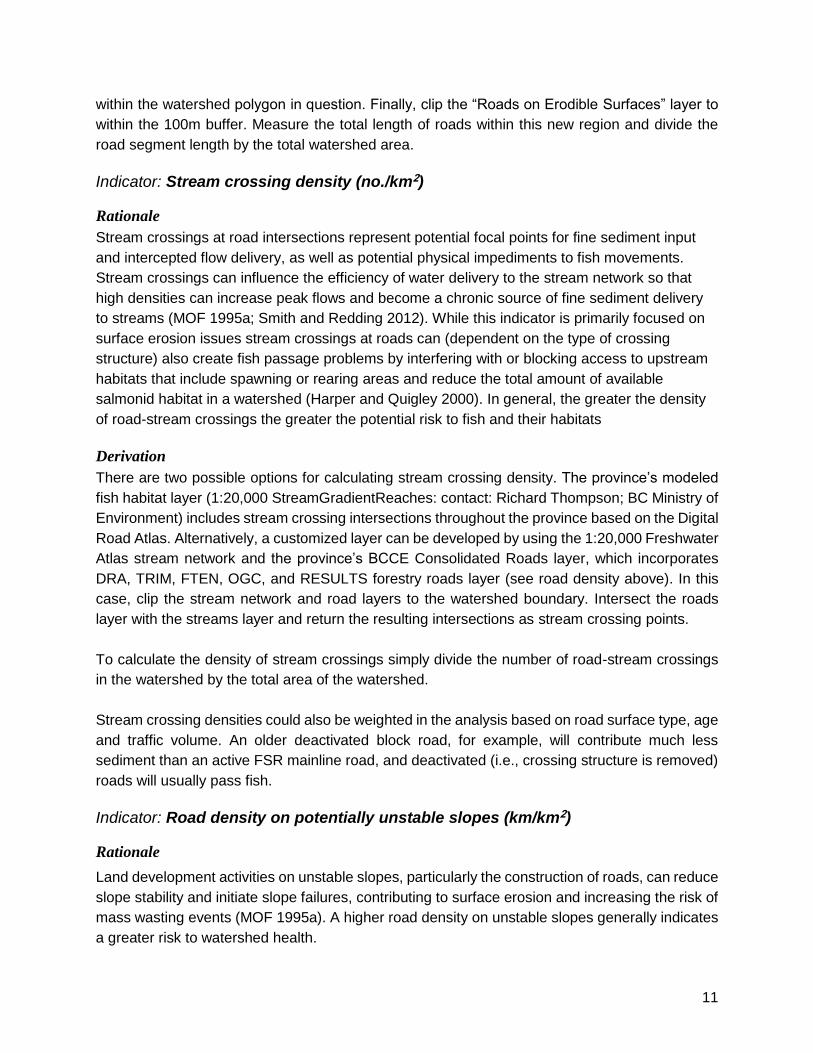
Indicator: Stream crossing density (no./km2)

Rationale

Stream crossings at road intersections represent potential focal points for fine sediment input

and intercepted flow delivery, as well as potential physical impediments to fish movements.

Stream crossings can influence the efficiency of water delivery to the stream network so that

high densities can increase peak flows and become a chronic source of fine sediment delivery

to streams (MOF 1995a; Smith and Redding 2012). While this indicator is primarily focused on

surface erosion issues stream crossings at roads can (dependent on the type of crossing

structure) also create fish passage problems by interfering with or blocking access to upstream

habitats that include spawning or rearing areas and reduce the total amount of available

salmonid habitat in a watershed (Harper and Quigley 2000). In general, the greater the density

of road-stream crossings the greater the potential risk to fish and their habitats

Derivation

There are two possible options for calculating stream crossing density. The province’s modeled

fish habitat layer (1:20,000 StreamGradientReaches: contact: Richard Thompson; BC Ministry of

Environment) includes stream crossing intersections throughout the province based on the Digital

Road Atlas. Alternatively, a customized layer can be developed by using the 1:20,000 Freshwater

Atlas stream network and the province’s BCCE Consolidated Roads layer, which incorporates

DRA, TRIM, FTEN, OGC, and RESULTS forestry roads layer (see road density above). In this

case, clip the stream network and road layers to the watershed boundary. Intersect the roads

layer with the streams layer and return the resulting intersections as stream crossing points.

To calculate the density of stream crossings simply divide the number of road-stream crossings

in the watershed by the total area of the watershed.

Stream crossing densities could also be weighted in the analysis based on road surface type, age

and traffic volume. An older deactivated block road, for example, will contribute much less

sediment than an active FSR mainline road, and deactivated (i.e., crossing structure is removed)

roads will usually pass fish.

Indicator: Road density on potentially unstable slopes (km/km2)

Rationale

Land development activities on unstable slopes, particularly the construction of roads, can reduce

slope stability and initiate slope failures, contributing to surface erosion and increasing the risk of

mass wasting events (MOF 1995a). A higher road density on unstable slopes generally indicates

a greater risk to watershed health.

12

Derivation

To determine locations for calculating road density on potentially unstable slopes employ terrain

mapping and slope stability classifications undertaken by registered professionals where such

exists. The potential for slopes to experience landsliding is determined by terrain (surficial

geology) mapping, and the subsequent interpretation of the terrain mapping information into slope

stability classes using, as defining criteria, slope angle, materials and landforms, material texture,

active geomorphological processes, and soil drainage (MOF 1995a). Detailed surficial geology

and terrain stability mapping, however, is currently available only for a subset of regions in BC so

it is not possible to classify areas of unstable slopes consistently across the province (D. Filatow,

pers. comm.). As an interim default measure, until broader terrain stability mapping is available

provincially, assume for analyses that all steep slopes (defined as >60% generally or >50% for

Haida Gwai watersheds as per guidance from PAETWG 2017) are considered unstable or

potentially unstable. Using a DEM, first isolate the areas within the watershed that are located on

steep slopes To do this, run a slope analysis using the DEM and reclassify the resulting raster file

to only those areas that represent slopes >60% (or >50%). Convert the reclassified slope raster

to polygon features and use this to calculate the total road length within the >60% (or >50%)

polygon. Divide this road length by the total watershed area.

Future deliverables from MOE (D. Filatow, pers. comm.) are expected to provide detailed mapping

of terrain stability characteristics across provincial watersheds. In the interim, estimates made

from SLC datasets that are available across the province could perhaps provide some additional

information for refining this stability indicator, but this would only be at a very coarse scale (i.e.,

1:2,000,000).

2.3.3 Indicator Category: Riparian Buffer

Indicator: Portion of streams logged (or otherwise disturbed) (km/km)

Rationale

Disturbances to riparian zones (i.e., land adjacent to the normal highwater line in a stream) can

affect fish habitats by destabilizing stream banks, increasing surface erosion and sedimentation,

reducing inputs of nutrients and woody debris, and increasing stream temperatures through

reduced streamside shading (Meehan 1991; MOF1995a). Riparian areas are intimately

connected with stream ecosystems, providing a wide variety of ecological services and functions.

The maintenance of these functions and services depends upon intact riparian areas. As the

portion of stream riparian areas that are logged increases, so does the risk of surface erosion and

mass-transport of sediment during heavy precipitation events. When riparian vegetation is

removed, stream channels are weakened due to the lack of root structures, and intensified surface

erosion and mass-wasting are common outcomes.

Derivation

Use the FAIB Consolidated Cutblocks layer to determine all areas indicated as having been

logged historically in the watershed. First, clip the Consolidated Cutblocks layer to within the

13

confines of the watershed to determine areas logged. Define additional areas disturbed by human

activities within the watershed boundaries by clipping out a composite of human disturbance

categories that are captured in the BCCE Provincial Development layers (i.e., rail, transmission,

mining, oil & gas, seismic, and urban activity), the province’s Baseline Thematic Mapper (BTM 1)

layer (i.e., harvesting, agriculture, and urban mixed activity), and the province’s Tantalis layer (i.e.,

major right of way corridors). Natural disturbances may also be included by extracting fire

perimeter polygons from the province’s current and historical fire layers, and insect disturbance

polygons from the province’s VRI layer.

Add the 1:20,000 Freshwater Atlas stream layer and clip to the watershed boundary. Intersect the

stream network with the logged and otherwise disturbed polygons (human and natural). To

calculate the portion of streams disturbed divide the total length of streams intersecting disturbed

polygons by the total length of streams within the watershed. A section of stream disturbed is

identified by locating disturbances that are immediately adjacent to or straddle a stream. The

underlying assumption for the analysis is that if a disturbed polygon is mapped as being

immediately adjacent to the stream or straddling the stream, then no riparian buffers were left (an

assumption that may not hold in many cases). An alternative, more complex but more accurate

method of calculating the extent of stream disturbance is presented in PAETWG (2017), involving

delineation of riparian buffer zone polygons (i.e., 30m width as default) and associated direct

measurement of disturbance levels within the defined buffer zone areas for a watershed.

Indicator: Portion of fish-bearing streams logged (or otherwise disturbed) (km/km)

Rationale

Disturbance of stream riparian zones will have potential impacts to fish and fish habitats (e.g.,

downstream effects on sediment and temperature) regardless of where they occur along the

stream network. However riparian disturbances in a watershed that directly overlap with fish-

bearing areas may be of greatest concern, as such disturbances could have a greater range of

direct and more intense localized impacts on fish populations.

Derivation

Follow the same steps as identified for calculating “Portion of streams disturbed”, but instead of

using the stream layer, use the province’s 1:20,000-based “FishAccessibleHabitat” GIS layer

(MOE contact: Richard Thompson, not yet available publicly on DataBC) or other reliable regional

fish distribution models if such exist, so that the subset of fish-bearing streams in the watershed

can be targeted for the calculation. In absence of such distribution modeling alternatively identify

stream reaches that are more than 100m in length and <20% grade and consider these as the

default criteria for defining fish habitat for assessments (L. Nordin, pers. comm.).

14

2.3.4 Indicator Category: Mass Wasting

Indicator: Stream banks logged (and otherwise disturbed) on steep slopes (km/km2)

Rationale

Stream banks disturbed on steep slopeshave potential for significant generation of surface

erosion and increased landslide potential, especially during heavy precipitation events. Sediment

transport, particularly of coarse material from mass wasting events, is largely a function of stream

gradient (MOF 2001). The steeper the gradient, the more material that moves down a stream

after it has entered a watercourse and the greater the distance of travel. Vegetation on slopes

intercepts precipitation and stabilizes surficial materials, and increased removal of vegetation on

slopes will affect watershed health and productivity.

Derivation

Use the Digital Elevation Model (DEM) to isolate all areas with steep slopes, defined as >60%

generally (or >50% for Haida Gwai watersheds as per guidance from PAETWG 2017). To do this

run a slope analysis using the DEM and reclassify the resulting raster file to only those areas that

represent slopes >60% (or 50%). To calculate density of stream banks disturbed on slopes >60%

(or 50%), determine the total length of streams have been disturbed (see Portion of Streams

Disturbed indicator above) on slopes >60% (or 50%) and divide this by the total watershed area.

Indicator: Density of landslides in the watershed (no./km2)

Rationale

The occurrence and frequency of occurrence of landslides within a watershed is an indication of

the presence of unstable slopes, with slope failures potentially linked to development activities in

the watershed (MOF 2001). Impacts from a slide into a stream can range from minor water quality

degradation to the initiation of a major debris torrent. Mass wasting events can be both beneficial

and detrimental to watersheds. Landslides can transport woody debris into streams, adding to

stream channel complexity which is favourable for spawning. Landslides can also harm fish-

bearing stream networks by introducing large quantities of coarse and fine sediment and creating

passage blocks. Landslide density should be monitored closely and in conjunction with many of

the indicators that focus on soil erosion, riparian logging, and unstable slopes.

Derivation

Landslide scars in a watershed can be identified using recent air photos or satellite imagery at a

scale of approximately 1:20,000, or through a direct aerial reconnaissance. Count any scar visible

at that scale as a landslide. Divide the number of landslides by the total watershed area.

There are no general provincial-scale GIS coverages of landslides within watersheds. There are

free Landsat, SPOT, and orthophoto data available for public access, but these should only be

used for general reference. This free data has unknown temporal frequencies, and only provides

partial coverage of the province. To conduct a change-detection strategy for evaluating landslide

15

occurrences within watersheds across the province, it will be necessary to purchase high

resolution satellite imagery. Although use of high resolution imagery can generate reliable results,

it can be expensive to obtain the imagery needed, especially on a repeat basis. It is suggested

that multiple parties purchase remote sensed imagery and split costs to increase the overall cost-

effectiveness of a change-detection method to monitor land slide events.

2.4 Future Tier 1 Indicators (climate change monitoring)

A warming and changing climate is likely to exacerbate existing watershed stresses from local

land management. While impacts to watersheds will likely vary depending on geographic location,

some potential increased risks to overall watershed condition could include:

• Warmer air and water temperatures

• Reduced snowpack

• Changes in seasonal precipitation (potentially more intense and concentrated)

• Changes in streamflow volume and seasonal timing (potentially higher in early spring,

lower in summer)

• Increased extent, intensity and frequency of wildfires (TRIG 2012)

A further set of potential indicators that could be used to reflect risk from climate change- induced

impacts have been identified for potential incorporation into the WSEP Tier 1 monitoring protocol:

Extent of snow/ice fields within watersheds

Snow field extent will have long term influences on water quantity, water quality (e.g., water

temperature), and timing of flow events; all critical factors for maintaining aquatic habitat

conditions. Mapping of changes in snow/ice field extents can be used to help evaluate potential

impacts from climate changes and will help in more accurately assessing the parallel effects of

local land management actions on watershed condition.

Base flows and water temperature:

Recent modeling by the BC MOE has identified regions of the province that are considered low

flow sensitive (either winter or summer flow sensitive, or both). This flow sensitivity has now been

mapped for large areas of the province (R. Ptolemy, pers. comm.) and this can be used as an

GIS overlay to identify provincial watersheds that may be most at risk from climate change effects

that could exacerbate low flow events. Modeled assessments of low flow risk will need to be

supplemented by real time monitoring of flows and water temperature in key watersheds using

permanent gauging at selected stream/river sites. Such gauging of key fisheries watersheds

should be designed to tie in with broader regional networks of stream flow and temperature

monitoring. Incorporating these (or other) climate change elements into the WSEP Tier 1

monitoring framework, determining related quantitative Indicators that can be measured and

tracked in this regard through remote sensed and/or field-based methods, and establishing key

benchmarks/thresholds of concern are elements to be developed in further iterations of the Tier

1 monitoring protocol.

16

2.5 Tier 1 indicator risk scores and overall assessment of

watershed status

Watershed assessment procedures applied in British Columbia have evolved over the years from

indicator threshold methods, to expert systems, to professional judgment approaches (Chatwin

2001). Since 2004, legislation around watershed assessments is driven by the Forest and Range

Practices Act (FRPA), where the decision to conduct watershed assessments is left to the

discretion of the forest licensee. In most cases, watershed assessments in BC conducted under

FRPA employ professional assessment approaches, while using 1999 WAP procedures (MOF

2001) as a general guide, modified to suit local conditions (Pike et al. 2007). Detailed professional

assessment approaches are unlikely to be a viable option, however, for regional/provincial scale

monitoring of status across large numbers of watersheds. WSEP Tier 1 assessments of the

overall status of watersheds will use a modified (and supplemented) version of the combined

indicator approach used in earlier provincial IWAP/CWAP procedures (MOF 1995a, b). These

WAPs used point scores of remote-sensed measures of watershed characteristics or land-use

patterns to assess the potential risk of impacts from forest harvesting or other disturbances to the

overall health of watersheds (Chatwin 2001). Selected indicators were intended to represent

proxies for watershed health.

As in the 1995 IWAP/CWAP procedures the WSEP Tier 1 evaluations will be based on combined

indicator scores for categories related to (1) peak flow, (2) sediment, (3) landslides, and (4)

riparian condition. Currently it is not possible to fully capture all the traditional IWAP/CWAP

indicators using the readily available provincial scale GIS coverages and remote sensed imagery

that will form the basis for broad Tier 1 monitoring. In the short term, provincial-scale GIS

data/coverages will need to be supplemented by local data sources in individual watersheds (if

and where available) to allow full capture of all WAP Indicators (if that is considered necessary or

desirable). For cases where there is a variable number of indicators available for use in a Tier 1

watershed assessment the rollup of indicators for evaluation of Impact Categories and overall

watershed risk status will have to be based on a potentially smaller set of input indicators. In these

cases, the intent would be to maintain the proportional elements within Impact Categories and

watershed rollup-ups for Tier 1 scoring, while also recognizing there will need to be some

adjustments based on the actual number of indicators available for calculation. This may affect

direct comparisons across watersheds. It is expected that it will be possible ultimately to

consistently calculate all traditional WAP indicators (and many others that it may be useful to

incorporate into an expanded WSEP Tier 1 protocol) across all BC watersheds using provincial-

scale datasets.

Risk scores for monitored indicators will be based (as a starting point) on indicator criteria used

within the standard IWAP/CWAP conversion tables (1995a, b). Examples of these IWAP/CWAP

conversion tables are provided in Appendix 1. Risk benchmarks of concern for each of the Tier 1

indicators to be used within provincially designated Fisheries Sensitive Watersheds (FSWs) or

other high value watersheds are to be set at lower indicator scores (i.e., more risk adverse) than

has been common practice in past provincial WAP assessments. So for example, while low risk

17

within a standard WAP would be defined as normalized indicator values <0.4, moderate risk at

normalized indicator values of 0.4 - 0.7, and high risk >0.7, low risk conditions for FSWs would

instead have normalized indicator values <0.2, moderate risk represented by normalized indicator

values of 0.2 - 0.4, and any normalized indictor value >0.4 would indicate high risk for that

indicator.

Assessment of these proposed more “risk-averse” Tier 1 indicator threshold values through an

expert-based survey (April 2012) of Fisheries Sensitive Watersheds Monitoring Technical

Working Group (FSW MTWG) members suggested that use of default 0.2 and 0.4 IWAP/CWAP

risk benchmarks provided a reasonable starting point in this regard. Survey participants generally

identified (within a range of variation) that the point at which they would expect detectable effects

on specific watershed functions occur near the WAP-defined 0.2 risk score, and indicator risk

scores of 0.4 were generally at the point where survey participants became concerned about

significant effects on watershed function (see Appendix 2 for results from this pilot benchmark

evaluation exercise). Further validation/refinement of indicator benchmarks of concern for Tier 1

monitoring will be developed through expanded, regionally specific (e.g., coastal vs. interior)

expert-based surveys/workshops of hydrologists, geomorphologists and fisheries biologists and

continuing interaction with the PAETWG. Such surveys could also be used to develop defensible

benchmarks for any new disturbance indicators that might be explored as part of the continuing

evolution of WSEP Tier 1 monitoring efforts and parallel exercises by the PAETWG. In the interim,

we suggest using IWAP or CWAP (as regionally appropriate) Level 1 assessment conversion

tables (MOF 1995a, b) indicator risk threshold scores of 0.2 and 0.4 as representing risk-adverse

Tier 1 benchmarks for defining low/moderate and moderate/high risk conditions respectively when

assessing condition of FWSs and other identified high priority watersheds.

WSEP Tier 1 watershed assessments are intended to be based on a two stage roll-up process:

1) a roll-up of the scored indicators (i.e., low, moderate, high risk scores relative to individual

benchmark values) within Impact Category risk classifications, and then 2) a rollup of the Impact

Category classifications into an overall watershed assessment risk classification. The appropriate

rollups to use in this regard have some level of subjectivity. The general intent is that all or most

(i.e., high proportion) of the nested indicators within an individual Impact Category (i.e., Peak

Flow, Surface Erosion, Riparian Buffer, Mass Wasting) would be defined as at low risk for the

Impact Category to also then be defined as at low risk. Similarly if all or most of the nested

indicators are defined as at high risk then the associated Impact Category should then also be

defined as at high risk.

A mix of low, moderate, and high risk categorizations across individual indicators would translate

to a moderate risk categorization for the associated Impact Category. Therefore a range of

potential combinations of indicator values could lead to different Impact Category classifications.

These potential combinations have not yet been fully explored or formalized but a survey of the

FSW MTWG in April 2012 suggested that an Impact Category should only be rated low risk if

approximately 75-80% or more of its associated (unweighted) indicators were scored at low risk

18

(this represents only a general rule as the sometimes small number of indicators related to a

particular impact category may not allow this specific percentage level resolution). The survey

also suggested that if > 50% of the nested indicators were at high risk then the Impact Category

should also be rated high risk. Identifying the various potential combinations of indicator scoring

that would result in a moderate risk classification for an Impact Category has not been finalized.

At the next level of the roll-up (i.e., Impact Categories to overall watershed assessment) the FSW

MTWG similarly suggested that at least 75% (i.e., 3 out of 4) of the Impact Categories must be

be rated as low risk for the overall watershed to be classified as low risk, and if 50% (i.e., 2 out of

4) or more of the Impact Categories were rated high risk then the overall watershed classification

should also be high risk. The various combinations of Impact Category scoring outside these

extremes that could result in an overall rating of moderate risk to a watershed have not yet been

formalized.

Determining agreed-to combinations of Impact Category scores that would represent moderate

risk ratings for watersheds and, similarly, combinations of nested indicator scores that would

represent moderate risk ratings for Impact Categories, may require development of approaches

such as expert-based survey analyses such as Discrete Choice Experiment – DCE, etc.) (e.g.,

Birol et al. 2006; Hoyos 2010) to better inform the exercise. Given the current lack of general

consensus within the FSW MTWG on the most defensible indicator roll-up approaches to use we

suggest in the interim that 1) watershed indicator assessment summaries may be presented as

simple summaries of individual indicator risk ratings, without grouping or roll-up into composite

Impact Categories or single Overall Watershed Assessment ratings, or 2) assessors develop

indicator roll-up algorithms that they think will be most defensible within their particular

assessment exercise.

Indicators within Impact Categories and Impact Categories within watersheds could be

considered either as being equally weighted or with a differential weighting element introduced.

Equal weighting may not be appropriate (in all or some cases) as particular Impact Categories

may have greater influence on overall watershed condition than others. Similarly, particular

indicators may reflect processes that have greater relative influence on particular Impact

Categories. There may be benefit to some level of differential weighting of indicators and/or

Impact Categories to more accurately reflect risk to watershed functions. An expert-based pilot

survey among the FSW MTWG in April 2012 suggested that weighting of Impact Categories and

their nested indicators could be appropriate to develop as a next step for refining watershed

scoring. Determining the appropriate quantitative weightings for these elements within the overall

watershed scoring would require a more comprehensive survey across a broader set of experts,

potentially employing structured decision approaches such as an Analytical Hierarchy Process –

AHP, etc. (e.g., de Steiguer et al. 2003; Barzekar et al. 2011).

Tier 2 monitoring (described in Pickard et al. 2014), intended for more intensive field-based

monitoring in a subset of selected watersheds, will be roughly comparable to the IWAP/CWAP

19

detailed field-based Level 3 assessments (MOF 1995a, b) of mass wasting, erosion, riparian

condition and stream channel stability. Tier 2 monitoring (Pickard et al. 2014) instead employs

field monitoring protocols developed for the province’s Forest and Range Evaluation Program

(FREP) (i.e., Riparian, Water Quality (modified) and Fish Passage protocols) (Carson et al. 2009;

MOE 2009; Tripp et al. 2009 respectively) with expansion of the sampling design approaches for

these protocols to allow for broader inferences of overall watershed condition. Tier 1 (remote-

sensed) information can be combined with analyses from Tier 2 (field-based) monitoring to

provide a composite “report card” of habitat pressures (i.e., risk) and condition within a watershed.

3.0 Next Steps / Recommendations

Continuing data collection and analysis from WSEP Tier 1 monitoring pilot studies (e.g., Porter et

al. 2015) will inform further development of the practical aspects of developing a broad scale,

remote sensed/GIS-based program of Tier 1 monitoring across the province’s FSWs and other

watersheds of concern. A full discussion of recommended elements in implementing a monitoring

program for FSWs and other watersheds at both the Tier 1 and Tier 2 level are described in the

workplan outlined in Pickard et al. 2009. Further steps in the continuing development of the Tier

1 protocol will be 1) discussions within the FSW MTWG and the PAETWG on finalizing

benchmarks of concern for individual Tier 1 indicators, and 2) establishing consistently defensible

indicator rollup algorithms that can will be used for overall assessments of watershed risk status

at the Tier 1 level.

4.0 Literature Cited B.C. Ministry of Environment (MOE). 2009. Field assessment for fish passage determination of

closed bottomed structures. 3rd Edition. May, 2009. B.C. Ministry of Environment, Victoria, BC.

B.C. Ministry of Forests (MOF). 1995a. Interior watershed assessment procedure guidebook (IWAP). http://www.for.gov.bc.ca/tasb/legsregs/fpc/fpcguide/iwap/iwap-toc.htm

B.C. Ministry of Forests (MOF). 1995b. Coastal watershed assessment procedure guidebook (CWAP). http://www.for.gov.bc.ca/tasb/legsregs/fpc/fpcguide/iwap/iwap-toc.htm

B.C. Ministry of Forests (MOF). 2001. Watershed Assessment Procedure Guidebook. 2nd ed., Version 2.1. For. Prac. Br., Min. For., Victoria, BC Forest Practices Code of British Columbia Guidebook. https://www.for.gov.bc.ca/tasb/legsregs/fpc/FPCGUIDE/wap/WAPGdbk-Web.pdf

Barzekar, G. A. Azi, M. Mariapan, M.H. Ismail, S.M Hosseni. 2011. Using Analytical Hierarchy Process (AHP) for prioritizing and ranking of ecological indicators for monitoring sustainability of ecotourism in Northern Forest, Iran. Ecologia Balkanica (3): 59-67.

Birol, E., K. Karousakis, and P. Koundouri. 2006. Using a choice experiment to account for preference heterogeneity in wetland attributes: The case of Cheimaditida wetland in Greece. Ecological Economics (60): 145-156.

Carson, B., D. Maloney, S Chatwin, M. Carver and P. Beaudry. 2009. Protocol for evaluating the potential impact of forestry and range use on water quality (Water Quality Routine

20

Effectiveness Evaluation). Forest and Range Evaluation Program, B.C. Ministry of Forest and Range and B.C. Ministry of Environment, Victoria, BC.

Chatwin, S. 2001. Overview of the development of IWAP from point scores to freeform analysis. In Watershed assessment in the southern interior of British Columbia. D.A.A. Toews and S. Chatwin (editors). B.C. Ministry of Forests, Research Branch, Victoria, B.C. Working Paper 57/2001, pp. 17–25.

de Steiguer, J.E.; Jennifer Duberstein, Vicente Lopes. 2003. The analytic hierarchy process as a means for integrated watershed management. In Renard, Kenneth G. First Interagency Conference on Research on the Watersheds. Benson, Arizona: U.S. Department of Agriculture, Agricultural Research Service. pp. 736–740.

Harper, D.J. and J.T. Quigley. 2000. No net loss of fish habitat: An audit of forest road crossings of fish-bearing streams in British Columbia, 1996-1999. Canadian Technical Report of Fisheries and Aquatic Sciences 2319. 43pp.

Hoyos, D. 2010. The state of the art of environmental valuation with discrete choice experiments. Ecological Economics (69): 1595-1603.

Hudson, R. and G. Horel. 2007. An operational method of assessing hydrologic recovery for Vancouver Island and south coastal BC. Research Section, Coast Forest Region, BC Ministry of Forests, Nanaimo, BC. Technical Report TR-032/2007.

Meehan, W.R. (ed.). 1991. Influence of Forest and Rangeland Management on Salmonid Fishes and Their Habitats. American Fisheries Society. Bethesda, Md. 751 pp.

Pickard, D., M. Porter, K. Wieckowski, and D. Marmorek. 2009. Workplan to Pilot the Fisheries Sensitive Watershed (FSW) Monitoring Framework. Report prepared by ESSA Technologies Ltd., Vancouver, BC. for BC. Ministry of Environment, Victoria.

Pickard, D., M. Porter, L. Reese-Hansen, R. Thompson, D. Tripp, B. Carson, P. Tschaplinski, T. Larden, and S. Casley. 2014. Fish Values: Watershed Status Evaluation, Version 1.0. BC Ministry of Forests, Lands and Natural Resource Operations and BC Ministry of the Environment (MOE), Victoria, BC.

Pike R.G., T. Redding, D. Wilford, R.D. Moore, G. Ice, M. Reiter, and D.A.A. Toews. 2007. Chapter 14 – Detecting and predicting changes in watersheds [Draft]. In Compendium of Forest Hydrology and Geomorphology in British Columbia [In Prep.] R.G. Pike et al. (editors). B.C. Ministry of Forests and Range Research Branch, Victoria, B.C. and FORREX Forest Research Extension Partnership, Kamloops, B.C. Land Management Handbook (TBD). URL: http://www.forrex.org/program/water/compendium.asp

Porter, M., S. Casley, N. Ochoski, and S. Huang. 2015. Watershed status evaluation: An assessment of 71 watersheds meeting BC’s Sensitive Watershed Criteria. Victoria BC FREP Report 39. http://www2.gov.bc.ca/assets/gov/farming-natural-resources-and-industry/forestry/frep/frep-docs/frep-fsw-watershedeval-2015.pdf

Porter, M., S. Casley, E. Snead, D. Pickard, and K. Wieckowski. 2019. Watershed Status Evaluation Protocol (WSEP): Tier 1 watershed-level fish values monitoring rationale. Version 3.2. March 2019.. Prepared by ESSA Technologies Ltd. for BC Ministry of the Environment (MOE) and BC Ministry of Forests, Lands, and Natural Resource Operations (FLNRO), Victoria, BC.

Province of British Columbia. 2016. Cumulative effects framework: Interim policy for the natural resource sector. Victoria, BC.

21

Provincial Aquatic Ecosystems Technical Working Group (PAETWG). 2017. Interim Assessment Protocol for Aquatic Ecosystems in British Columbia. Version 1.1 (Dec. 2017). Prepared for the Ministries of Environment and Forests, Lands and Natural Resource Operations Value Foundation Steering Committee.

Sawyer, M.D., Mayhood, D.W. 1998. Cumulative effects analysis of land-use in the Carbondale River catchment: Implications for fish management. Pages 429-444 in M.K. Brewin and D.M.A. Monita, tech. cords. Forest-fish conference: land management practices affecting aquatic ecosystems.

Smith, R.S., R.A. Scherer, and D.A. Dobson. 2008. Snow cover extent during spring snowmelt in the south-central interior of British Columbia. BC Journal of Ecosystems and Management 9(1): 57-70.

Smith, R. and T. Redding. 2012. Cumulative effects assessment: Runoff generation in snowmelt-dominated montane and boreal plain catchments. Streamline Watershed Management Bulletin 15(1): 24-34.

The Resource Innovation Group (TRIG). 2012. Towards a resilient watershed: Addressing climate change planning in watershed assessments. Report prepared for the Oregon Watershed Enhancement Board.

Tripp, D.B., P.J. Tschaplinski, S.A. Bird and D.L. Hogan. 2009a. Protocol for evaluating the condition of streams and riparian management areas (Riparian Management Routine Effectiveness Evaluation). Forest and Range Evaluation Program, B.C. Min. For. Range and B.C. Min. Env., Victoria, BC.

Winkler, R. and S. Boon. 2015. Revised snow recovery estimates for pine-dominated forests in interior British Columbia. Province of B.C., Victoria, B.C.,Extension Note 116.

22

Appendix 1 Comparison of Watershed Status Evaluation Protocol (WSEP) and the Aquatic Cumulative Effects Framework protocol (ACEF).

WSEP ACEF

General purpose of protocols

Fish habitat focused assessment to understand the pressures on (Tier 1), and condition of (Tier 2), legally designated FSW’s, watersheds with significant fish values, and to help provide improved management direction as required.

General assessment of pressures on all (standardized) watershed-based analysis units in BC.

Monitoring question being addressed

Are there significant risks to the watershed (Tier 1)? What is the ‘real-world’ condition of the watershed`s fish habitat (Tier 2)? What can be done to improve watershed condition if necessary?

What is the extent of pressures on watersheds in BC (affecting Water Quality, Water Quantity, and Riparian Habitat)? How are they changing over time?

Indicators Uses 8 to 9 Tier 1 indicators derived from BC Watershed Assessment Procedure. Also uses several BC condition monitoring protocols.

Uses 6 Tier 1 indicators from BC Watershed Assessment Procedure.

Assessment Units Uses targeted watersheds with legal boundaries or natural watershed boundaries. WSEP assessment units do not conform to CEF analysis units.

Uses ~19,000 permanently defined and similarly sized watershed assessment units across BC. In some cases assessment units are aggregates of adjacent watersheds.

Analysis of indicators

Tier 1: standalone interpretation of each specific (up to 9) pressures/ risks indicator in a watershed of interest (e.g. density of roads in a watershed). Tier 2: uses field-based stream channel, riparian, water quality and fish passage condition protocols. Tier 1 & II together are used to assess a watershed’s status.

A tool used to address pressure/risk in an analysis unit by rolling up all indicator values into an overall score for component and value for each analysis unit.

Benchmarks (risk reference points)

Set as precautionary associated with high fish values within target watersheds.

Set more moderately since protocol is applied generically across all BC analysis units.

Results inform (i) Strategic direction for effectiveness monitoring and (ii) operational/management recommendations for sustainable management outcomes.

Strategic information to prioritize subsequent information gathering and inform conversations (e.g. regional) on the state of watersheds (e.g. land-use planning).

23

Appendix 2 IWAP and CWAP Level 1 assessment conversion tables (Tables A2a (interior) and A2b (coastal) for scoring WAP indicator values*. These provide the base scoring framework for WSEP Tier 1 assessments.

Table A1a. Interior watershed assessment conversion table (from MOF 1995a).

24

Table A1b. Coastal watershed assessment conversion table (from MOF 1995b).

* Typically, low risk within IWAPs/CWAPs has been defined as indicator scores < 0.4 or 0.5, moderate risk at scores of 0.4 or 0.5 - 0.7, and high risk for scores >0.7. Scoring for Fisheries Sensitive Watersheds (FSW) and other priority watersheds will be intended to be somewhat more risk adverse for these designated watersheds, with low risk likely being defined as indicator scores < 0.2, moderate risk at 0.2 -0.4, and high risk for scores > 0.4.

25

Appendix 3 Range across survey participants (n = 7) at an April 2012 FSW MTWG meeting for the values for a subset of Tier 1 indicators at which they: A) would expect detectable effects on specific watershed functions, and B) would begin to have significant concerns in regard to specific watershed functions. Related WAP risk scores of 0.2 (the suggested default Tier 1 moderate risk benchmark) and 0.4 (the suggested default Tier 1 high risk benchmark) are shown in each figure for comparison.

A

B

26

A

B

27

A

B