WAVE FORCES ON BRIDGES Mary-Margaret Dickey

WAVE FORCES ON BRIDGES

By

Mary-Margaret Dickey

A Thesis Submitted to the Faculty of Mississippi State University

in Partial Fulfillment of the Requirements for the Degree of Masters of Science

in Civil and Environmental Engineering in the Department of Civil and Environmental Engineering

Mississippi State, Mississippi

December 2008

Copyright by


2008

WAVE FORCES ON BRIDGES

By


Approved:

Philip M. Gullett William H. McAnally Assistant Professor of Civil and Associate Professor of Civil and Environmental Engineering Environmental Engineering (Director of Thesis) (Committee Member)

R. Ralph Sinno James L. Martin Professor of Civil and Environmental Professor and Graduate Coordinator of Engineering Civil and Environmental Engineering (Committee Member)

Sarah A. Rajala Dean of Bagley College of Engineering

Name: Mary-Margaret Dickey

Date of Degree: December 12, 2008

Institution: Mississippi State University

Major Field: Civil and Environmental Engineering

Major Professor: Dr. Philip M. Gullett

Title of Study: WAVE FORCES ON BRIDGES

Pages of Study: 76

Candidate for Degree of Master of Science

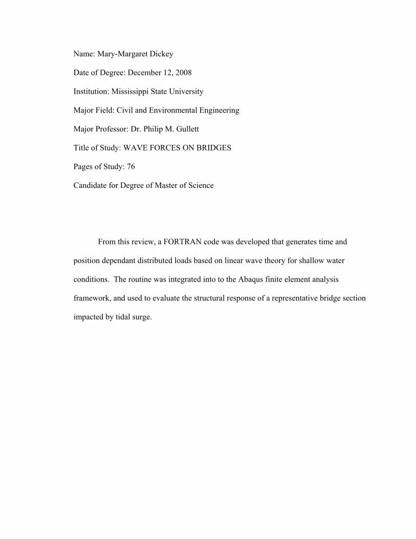
From this review, a FORTRAN code was developed that generates time and

position dependant distributed loads based on linear wave theory for shallow water

conditions. The routine was integrated into to the Abaqus finite element analysis

framework, and used to evaluate the structural response of a representative bridge section

impacted by tidal surge.

TABLE OF CONTENTS

Page

LIST OF TABLES............................................................................................................. iv

LIST OF FIGURES .............................................................................................................v

CHAPTER

I. INTRODUCTION ................................................................................................1

Background...........................................................................................................1 Objectives & Tasks ...............................................................................................2 Scope.....................................................................................................................5

II. LITERATURE REVIEW .....................................................................................6

Denson ..................................................................................................................6 Wave Forces on Causeway-Type Coastal Bridges........................................6 Wave Forces on Causeway-Type Coastal Bridge: Effects of Angle of

Wave Incidence and Cross-Section Shape................................................7 Pressures on Coastal Bridges Due to Normal Incidence Waves ...................8

Morison, et al. .......................................................................................................9 Bea, et al..............................................................................................................10 Douglass, et al.....................................................................................................11 McConnell, et al..................................................................................................13

III. USER SUBROUTINE........................................................................................16

Introduction.........................................................................................................16 Standard Abaqus .................................................................................................17

Input File .....................................................................................................17 Common.h ...................................................................................................18 DLOAD .......................................................................................................19 UEXTERNALDB .......................................................................................19

Specialized Abaqus.............................................................................................20 Element.dat..................................................................................................20

Wave Force Subroutine.......................................................................................21 Surface Forces- Horizontal and Vertical .....................................................22 Buoyancy.....................................................................................................24

ii

Page

Wave Force Check..............................................................................................28

IV. NUMERICAL SIMULATION...........................................................................29

Introduction.........................................................................................................29 Model ..................................................................................................................30

Simple Block ...............................................................................................31 Geometry..............................................................................................31 Material Properties...............................................................................32 Boundary Conditions ...........................................................................33

Load .....................................................................................................33 Bridge Deck.................................................................................................34

Geometry..............................................................................................34 Material Properties...............................................................................35 Boundary Conditions ...........................................................................36

Load .....................................................................................................37 Response of Structure .........................................................................................38

Simple Block ...............................................................................................38 Bridge Deck.................................................................................................39

V. CONCLUSIONS.................................................................................................42

REFERENCES ..................................................................................................................44

APPENDIX

A. USER SUBROUTINES......................................................................................46

B. SIMPLE BLOCK EXAMPLE............................................................................54

C. FIXED BRIDGE EXAMPLE.............................................................................60

D. SIMPLY-SUPPORTED BRIDGE EXAMPLE..................................................62

E. ABAQUS TUTORIAL .......................................................................................64

F. ABAQUS/WAVE FORCE STEPS.....................................................................75

iii

LIST OF TABLES

TABLE Page

2.1 Douglass Force Estimates from Literature for Case Study: Biloxi Bay August 29, 2005 at 8:00 am .................................................................12

3.1 Coefficients .........................................................................................................23

3.2 Wave Characteristics ..........................................................................................24

3.3 Scale Factors for Buoyancy ................................................................................26

3.4 Wave Force Check Results .................................................................................28

4.1 Wave Characteristics for Simple Block..............................................................38

iv

LIST OF FIGURES

FIGURE Page

1.1 Biloxi Bay Bridge (Looking West)..........................................................................3

1.2 Biloxi Bay Bridge (Looking East) ...........................................................................4

2.1 Definition of Force Parameters (McConnell et al. 2003) ......................................14

3.1 Abaqus Analysis with Wave Force Schematic ......................................................17

3.2 Element.dat Format and Explanation.....................................................................21

3.3 Wave Profile (Kerenyi 2005).................................................................................25

3.4 The Cases for Buoyancy ........................................................................................27

4.1 Simple Block..........................................................................................................32

4.2 Stress-Strain Curve of Concrete.............................................................................33

4.3 Bridge Model’s Cross-section................................................................................34

4.4 Girder Cross-section ..............................................................................................35

4.5 Bridge Abaqus Solid Model...................................................................................37

4.6 Fixed Bridge Model ...............................................................................................40

4.7 Simply-Supported Bridge Model at T=3.0 s..........................................................41

4.8 Simply-Supported Bridge at T=6.0 s .....................................................................41

v

CHAPTER I

INTRODUCTION

Background

A bridge is a structure built to span a gorge, valley, road, railroad track, river,

body of water, or any other physical obstacle (Wikipedia March 1, 2008). Bridges are

designed to carry many different types of loads. Foremost, they are designed for

vehicular loading and gravity. Then, depending on their location, they are designed for

loads caused by water, wind, ice, and earthquakes.

Low-lying bridges along coastlines may be subject to loading from waves and

surge. The American Association of State Highway and Transportation Officials

(AASHTO) Load Resistance Factor Design (LRFD) Bridge Design Specifications gives

this guidance: “Wave action on bridge structures shall be considered for exposed

structures where the development of significant wave forces may occur” (AASHTO

2006). It references the Shore Protection Manual for computing the wave forces given

the site-specific conditions. This manual provides guidelines for computing forces

created by waves on pilings and walls but gives no aid for bridge’s superstructure.

Moreover the manual is intended for users with a background in ocean mechanics and

much of the content is unfamiliar to structural engineers designing bridge road way

structures. There are current design codes for coastal structures which give a guideline

1

for forces; however, Yim characterizes these approaches as “often grossly simplified and

may be overly conservation [sic] and/or unreliable.(Yim 2005)”

Due to the lack of design guidelines for wave forces many bridge road way

structures have been severely damaged or destroyed. In 1969, Hurricane Camille

damaged the Biloxi Bay and the Bay St. Louis bridges. In 1979, Hurricane Frederic

caused the Dauphin Island Causeway to fail. In 2004, Hurricane Ivan removed several

sections of the I-10 Escambia Bay Bridge from its pilings. In 2005, Hurricane Katrina

damaged the US Hwy 90 Biloxi Bay and Bay St. Louis bridges beyond repair along with

damage to the I-10 Lake Pontchartrain and Mobile Bay bridges. The loss of these bridges

after Hurricane Katrina resulted in major disruptions in transportation, making it difficult

for emergency assistance and rescue to coordinate without undo delays. It is estimated to

have taken three hundred and thirty-eight million dollars to replace the Biloxi Bay Bridge

(Bergeron 2007). The lost of this bridge only added to the lengthy economical recovery.

To prevent these disruptions and costs, design guidance for coastal bridges is needed-

whether retrofitting for existing bridges or designing future bridges. Just as water, wind,

ice, and earthquakes have design specifications there should also be a design

specification for wave loads due to water surge in a hurricane.

Biloxi Bay Bridge is located along one of the two main east-west corridors for

Mississippi’s gulf coast, U.S. Hwy. 90, connecting Biloxi to Ocean Springs. Before

Hurricane Katrina halted it’s use, traffic counts were approximately 30,000 average daily

traffic, ADT, annually (MDOT 2006). Surrounding most of the bridge, the water depth is

very shallow, 2’ to 3’, except for the shipping channel, 11’ to 12’(Douglass et al. 2006).

The superstructure of the bridge was made up of prestressed concrete girders with a cast-

2

in-place reinforced concrete deck, with each section being 52’ by 33.4’. The bridge was

simply supported by pile caps on either end. Between the girders and the pile caps were

bearing pads that provided no resistance to uplift.

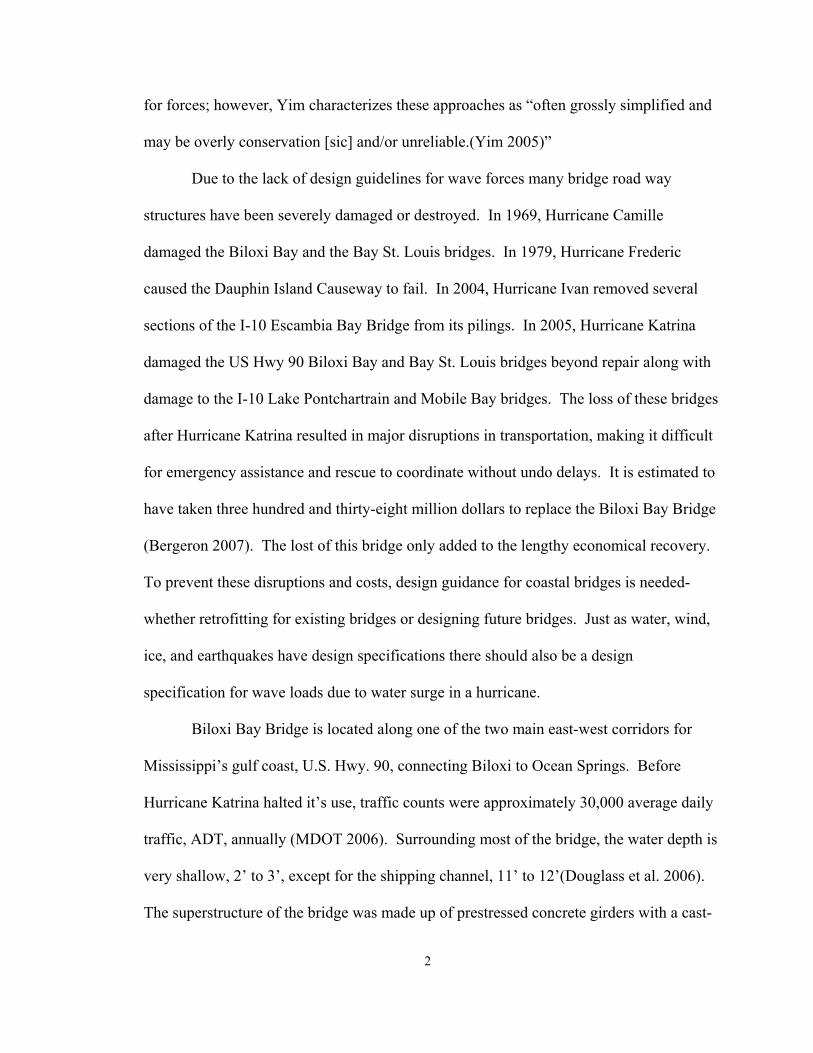
The loading created by Hurricane Katrina’s wave surge caused most of the spans

to be displaced. Some were completely moved off of the pile caps and came to rest 16’

to 47’ away (O'Connor 2005). In some cases, the girders and the deck sustained

significant fracturing. The elevated spans that led to the drawbridge were the only ones

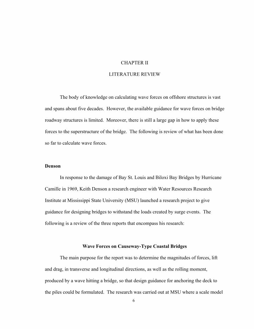
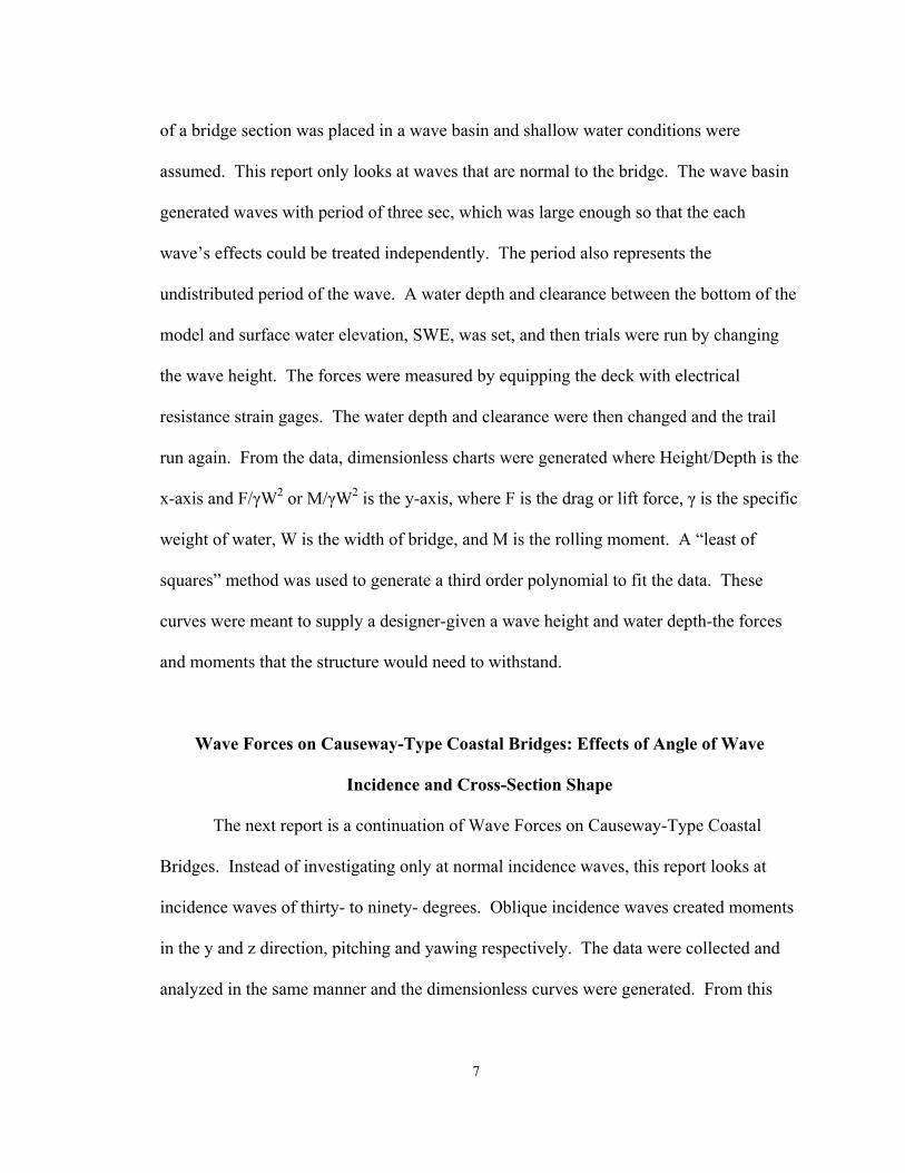
not damaged or moved, being out of the waves’ reach. See Figures 1.1 and 1.2.

Figure 1.1

Biloxi Bay Bridge (Looking West)

3

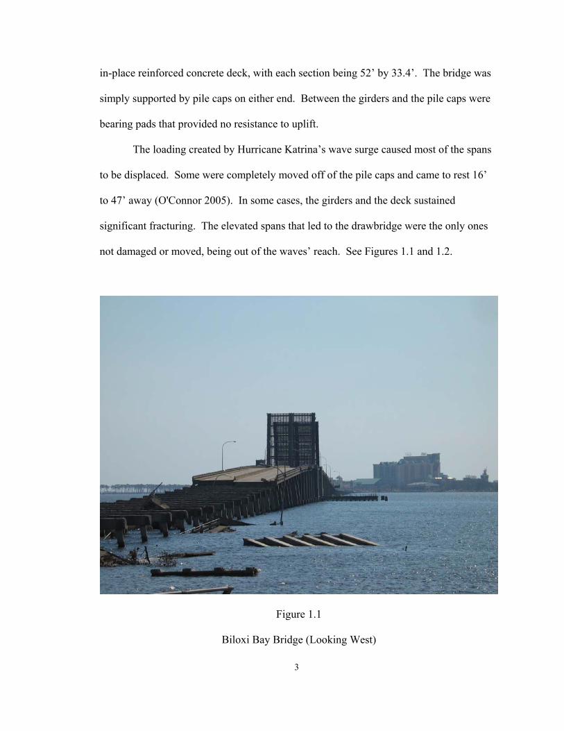
Robertson suggests that friction from the structures self-weight and small thick

steel angles were the only restraints to the lateral movement. The lack of restraint plus

the forces of uplift and buoyancy, allowed the structure to move off of its substructure,

the piling (Robertson et al. 2007). Douglass suggests that the damaging agent was the

wave-induced loads from the wave crest hitting the un-submerged bridge deck (Douglass

et al. 2006). Both agreed that its simply supported design led to its failure.

Figure 1.2

Biloxi Bay Bridge (Looking East)

4

Objectives & Tasks

The purpose of this study is to make [a first order approximation of the structural

response of a bridge deck subjected to a normal incidence wave.] The tasks to

accomplish are as follows:

1. Formulate FORTRAN code for wave force calculation.

2. Determine appropriate coefficients and wave characteristics.

3. Develop model of a bridge: fixed and simply supported.

4. Interface code and model.

5. Compare results with damage of U.S. Hwy 90 Biloxi Bay Bridge.

6. Make Recommendations

Scope

This study consists of developing a finite element model of a simple support and

fixed bridge sections and applying wave loads to the section in order to better understand

bridge-wave interaction. The bridge section is representative of the Biloxi Bay Bridge

with some simplifications which will be discussed in Chapter 3.

Abaqus/Standard was selected using DLOAD subroutine for wave force

calculation. The wave force calculation was based on Morison’s equation (Kerenyi 2005;

Morison et al. 1950) using linear wave theory to calculate the water particle velocities.

The subroutine does not take into account wind, debris, scour, or trapped air. In the

analysis, the wave force loading will vary with time, so that the full picture of the

bridge’s reaction to the wave will be generated.

5

CHAPTER II

LITERATURE REVIEW

The body of knowledge on calculating wave forces on offshore structures is vast

and spans about five decades. However, the available guidance for wave forces on bridge

roadway structures is limited. Moreover, there is still a large gap in how to apply these

forces to the superstructure of the bridge. The following is review of what has been done

so far to calculate wave forces.

Denson

In response to the damage of Bay St. Louis and Biloxi Bay Bridges by Hurricane

Camille in 1969, Keith Denson a research engineer with Water Resources Research

Institute at Mississippi State University (MSU) launched a research project to give

guidance for designing bridges to withstand the loads created by surge events. The

following is a review of the three reports that encompass his research:

Wave Forces on Causeway-Type Coastal Bridges

The main purpose for the report was to determine the magnitudes of forces, lift

and drag, in transverse and longitudinal directions, as well as the rolling moment,

produced by a wave hitting a bridge, so that design guidance for anchoring the deck to

the piles could be formulated. The research was carried out at MSU where a scale model

6

of a bridge section was placed in a wave basin and shallow water conditions were

assumed. This report only looks at waves that are normal to the bridge. The wave basin

generated waves with period of three sec, which was large enough so that the each

wave’s effects could be treated independently. The period also represents the

undistributed period of the wave. A water depth and clearance between the bottom of the

model and surface water elevation, SWE, was set, and then trials were run by changing

the wave height. The forces were measured by equipping the deck with electrical

resistance strain gages. The water depth and clearance were then changed and the trail

run again. From the data, dimensionless charts were generated where Height/Depth is the

x-axis and F/γW2 or M/γW2 is the y-axis, where F is the drag or lift force, γ is the specific

weight of water, W is the width of bridge, and M is the rolling moment. A “least of

squares” method was used to generate a third order polynomial to fit the data. These

curves were meant to supply a designer-given a wave height and water depth-the forces

and moments that the structure would need to withstand.

Wave Forces on Causeway-Type Coastal Bridges: Effects of Angle of Wave

Incidence and Cross-Section Shape

The next report is a continuation of Wave Forces on Causeway-Type Coastal

Bridges. Instead of investigating only at normal incidence waves, this report looks at

incidence waves of thirty- to ninety- degrees. Oblique incidence waves created moments

in the y and z direction, pitching and yawing respectively. The data were collected and

analyzed in the same manner and the dimensionless curves were generated. From this

7

research, Denson determined that normal incidence waves created the most severe

conditions for the bridge.

Pressures on Coastal Bridges Due to Normal Incidence Waves

From his previous report, Denson choose to determine the pressures created by

the critical angle of incidence, ninety-degrees. Here, pressures were measured at five

discrete points along the width of the scale bridge (perpendicular to flow of traffic and

parallel to wave action) also varying wave height and depth. Then the data were

examined and the peak negative and positive pressures were isolated since the time

between them was “so short as to be practically indiscernible”(Denson 1981). Then, it

was put into dimensionless form by the function p/GH, where p is water pressure

measured at the underside of the deck, G is specific weight of water, H is wave height. It

was put into dimensionless form to “normalize the pressure with respect to wave height

in order to possible [sic] obtain a more general relationship”(Denson 1981). Denson

observed that pressure was a linear function of wave height. Also that the wave produced

a positive uplift, from the crest’s passing, followed by a down-pull (suction), from the

trough’s passing. Denson observed overwash of the seaward lane. Overwash is when

part of the wave splashes over the bridge. He determined overwash to be a function of

bridge height to water depth ratio. Denson believed that a combination of loading from

overwash and pressure should be used to determine maximum loading. He intended that

the dimensionless data be used to design bridges for this maximum loads. Again he

created curves that were the dimensionless function vs. location of the electrical

resistance strain grains to bridge width ratio, with these tables the design engineer could

8

enter the curves with the appropriate line (H/D) and pick out the peak positive and

negative p/GH and the multiply by G and H to get the pressure for the prototype.

However, these curves are not clear enough-- it is hard to tell the H/D lines apart.

There are some issues with these reports that have kept them from being used as a

design tool. First, the curves are cumbersome to use because of their dimensionless form.

Second, the research is only relative for bridges with the same cross-section. Third,

buoyancy and the overwash force are not addressed in the research. Douglass, et al.

suggest that the wave period Denson used were not realistic for Biloxi Bay during a

hurricane (Douglass et al. 2006). However, it is the only completed work for measuring

forces on a bridge section.

Morison, et al.

Morison derived wave forces equations by using linear wave theory and

transitional water depth that were applicable to pilings. The equations were verified by

an experimental study. He determined that there were two components of the force: “a

drag force proportional to the square of the velocity which may be represented by a drag

coefficient having substantially the same value as for the steady flow” and “a virtual mass

force proportional to the horizontal component of the accelerative force exerted on the

mass of water displaced by the pile” (Morison et al. 1950). However, Morison cautioned

that these results were applicable to only single piles.

9

Bea, et al.

Bea, et al. research dealt with modifying the American Petroleum Institute (API)

Supplement 1 guidelines for computing the maximum horizontal forces generated by

wave crests for offshore oil platforms. The research was based on laboratory test model

results and by platforms performance during past hurricanes. Bea formulates the total

force (Ftw) from a wave crests impact as follows:

Ftw = Fb + Fs + Fd + Fl + Fi (2.1)

Where, Fb is buoyancy force, Fs is the slamming force, Fd is the drag force, Fl is lift force

and Fi is the inertia force. Bea uses the Morison formulation to calculate the deck forces.

The slamming force is:

Fs = 0.5ρCs Au2 (2.2)

Where, Cs is the slamming coefficient, ρ is the mass density of seawater, A is the vertical

deck area and u is the horizontal fluid velocity. The drag force is given by:

Fd = 0.5ρCd Au2 (2.3)

Where, Cd is the drag coefficient. The vertical lift force is given by:

Fl = 0.5ρCl Au2 (2.4)

Where, Cl is lifting coefficient. The inertial force is given by:

Fi = ρCmVa (2.5)

Where, Cm is the inertia coefficient, V is the volume of the deck submerged and a is the

water acceleration. Bea account for the platform deck’s response with an “effective”

slamming force that is given by:

10

Fs ' = FeFs (2.6)

Where Fe is a dynamic loading factor and Fs is given as above.

Bea used Stokes fifth order theory to calculate the velocities - given a wave height

and wave period. The work is empirically based. Bea concluded that the modified

procedure produced results that represented the failures seen in the field better than the

API procedure, which produced very conservative results. API “predicts failures when

only minor damage or no damage was observed.” (Bea et al. 1999)

Douglass, et al.

Douglass, et al. gives a history of what has been done in the past to generate wave

forces. Douglass formulates a simple-to-apply and conservative interim guidance for

calculating wave forces based on the available knowledge. The vertical and horizontal

components of forces (Fv and Fh, respectively) are:

F = c F * (2.7)v v−va v

and

Fh = [1+ cr (N −1)]ch−va Fh (2.8)

Where, cv-va is an empirical coefficient for the vertical varying load, Fv* is a reference

vertical load, cr is a reduction coefficient for the horizontal varying load, N is the number

of girders supporting the bridge span deck, ch-va is an empirical coefficient for the

horizontal varying load, and Fh* a reference horizontal load. Fv

* and Fh*are as follows:

Fv * = γ (∆z)Av (2.9)

and

11

Fh * = γ (∆z)Ah (2.10)

Where, γ is the unit weight of water, Av and Ah are the areas of the bridge projection into

the horizontal/vertical plane, ∆zv is difference between the elevation of the crest of the

maximum wave and the elevation of the underside of the bridge deck, ∆zh difference

between the elevation of the crest of the maximum wave and the elevation of the centroid

of Ah.

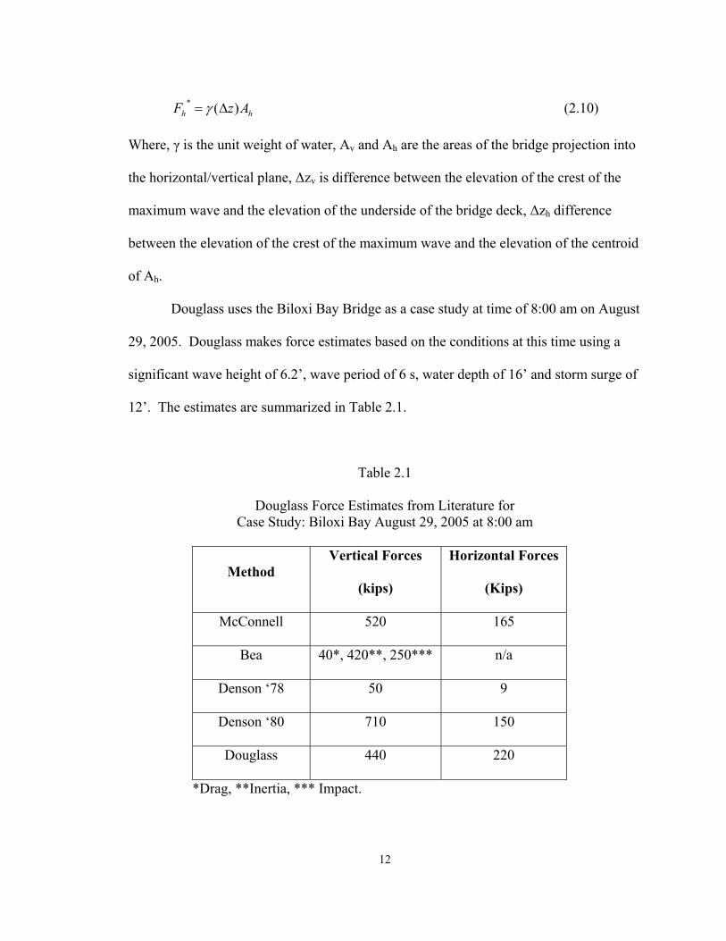
Douglass uses the Biloxi Bay Bridge as a case study at time of 8:00 am on August

29, 2005. Douglass makes force estimates based on the conditions at this time using a

significant wave height of 6.2’, wave period of 6 s, water depth of 16’ and storm surge of

12’. The estimates are summarized in Table 2.1.

Table 2.1

Douglass Force Estimates from Literature for Case Study: Biloxi Bay August 29, 2005 at 8:00 am

Method Vertical Forces

(kips)

Horizontal Forces

(Kips)

McConnell 520 165

Bea 40*, 420**, 250*** n/a

Denson ‘78 50 9

Denson ‘80 710 150

Douglass 440 220

*Drag, **Inertia, *** Impact.

12

Douglass chose this as the case study because it had the most reliable results,

unlike choosing the worst case when the bridge was submerged. Douglass suggests that

the values above account for the damage seen at Biloxi Bay Bridge, given its self-weight

was 340 kips. He concludes that the trapping of air added to its buoyancy. Douglass also

describes the vertical loading as slowly varying force able to move the spans in the down-

wave direction. However, not addressed in Douglass’s research is a method for applying

the interim guidance loads onto the bridge superstructure.

McConnell, et al.

HR Wallingford undertook the exposed jetties research project due to the need of

the trade industry to be able to build jetties in exposed locations without breakwater

protection. This research encompassed performing model tests of a scaled deck with and

without beams. The model was placed in a wave flume that was capable of creating

random waves. The model was also fitted with four force transducers to record force

measurements. A typical time series of forces created as a wave hit the model is shown

in Figure 2.1.

13

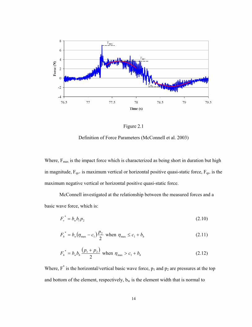
Figure 2.1

Definition of Force Parameters (McConnell et al. 2003)

Where, Fmax is the impact force which is characterized as being short in duration but high

in magnitude, Fqs+ is maximum vertical or horizontal positive quasi-static force, Fqs- is the

maximum negative vertical or horizontal positive quasi-static force.

McConnell investigated at the relationship between the measured forces and a

basic wave force, which is:

F * = b b p (2.10)v w l 2

Fh * = bw (ηmax − c1 )

p2 when ηmax ≤ c1 + bh (2.11)2

(p + p )* 1 2F = b b when η > c + bh (2.12)h w h max 12

Where, F* is the horizontal/vertical basic wave force, p1 and p2 are pressures at the top

and bottom of the element, respectively, bw is the element width that is normal to

14

direction of wave attack, bh is element depth, c1 is clearance, and ηmax is the maximum

wave crest elevation relative to still water level (SWL).

The ratio of quasi-static force to the basic wave force was plotted versus a ratio of

maximum wave elevation minus the clearance to maximum wave height. The latter

accounts for the incident wave conditions and geometry. This was carried out for both

vertical and horizontal forces and for an interior and exterior beam. To predict quasi-

static forces, a best fit regression line was fitted for each plot, with the following general

form of:

F a F

qs * = ) b (2.13)

⎡(η − c ⎤max 1⎢ ⎥H⎣ s ⎦

Where, F* is the basic wave force, c1 is the clearance between soffit level and SWL, ηmax

is the maximum wave crest elevation, and a and b are coefficients. See McConnell for

values of a and b.

McConnell determined that the internal elements varied from the external

elements in some cases because they were “influenced by the decks configuration”. Also

concluded that the vertical upward acting force, Fvqs+, was caused by the slam of the

bottom of the deck or beam, the vertical downward acting force, Fvqs-, was caused by

inundation of the deck, the horizontal landward acting force, Fhqs+, cause by the wave

impacting the beam, and the horizontal landward force, Fhqs-, caused by the wave

impacting the back of the beam due to trapping of wave by the deck.

15

CHAPTER III

USER SUBROUTINE

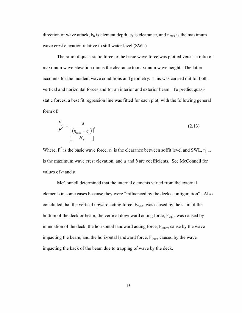
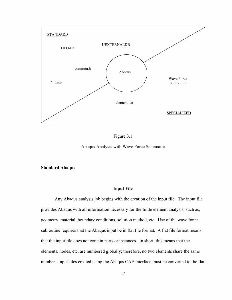
Introduction

An Abaqus analysis run with Wave Force subroutine requires specialization in

input information and requires the following files (See Figure 3.1):

1. Abaqus Input File (*_f.inp)

2. Element.dat

3. Common.h

4. Wave Force Subroutine

a. Source.f

b. Surfaceforce.f

c. Bodyforce.f

d. Parameters.dat

16

STANDARD

UEXTERNALDB DLOAD

common.h Abaqus

Wave Force *_f.inp Subroutine

element.dat

SPECIALIZED

Figure 3.1

Abaqus Analysis with Wave Force Schematic

Standard Abaqus

Input File

Any Abaqus analysis job begins with the creation of the input file. The input file

provides Abaqus with all information necessary for the finite element analysis, such as,

geometry, material, boundary conditions, solution method, etc. Use of the wave force

subroutine requires that the Abaqus input be in flat file format. A flat file format means

that the input file does not contain parts or instances. In short, this means that the

elements, nodes, etc. are numbered globally; therefore, no two elements share the same

number. Input files created using the Abaqus CAE interface must be converted to the flat

17

file format. This is accomplished by adding the following to the Abaqus environment file

(Abaqus_*.env, *indicates the version of Abaqus):

print_flattened_file=ON

def onJobCompletion():

import os,osutils

if os.path.exits('%s_f.inp'%id):

src='%s_f.inp'%(id)

dest=savedir

if os.path.exists("%s_f.pes'%id):

src='%s_f.pes'%(id)

dest=savedir

osutls.copy(src,dest)

Common.h

Common.h sets aside the memory needed for interfacing between Abaqus and

Wave Force subroutine. Common.h is in common block format; it contains parameters

defined by the user and Abaqus through UEXTERNALDB to be used by DLOAD for

wave force calculation. UEXTERNALDB and DLOAD will be discussed later in the

chapter. The main reason common.h is used is to simplify the Wave Force subroutine

code. In common.h file, JSURFELEMENTS and NUM_ELS, must be supplied by the

user and will be discussed in depth later. See Appendix for common.h.

18

DLOAD

DLOAD is a user subroutine available in Abaqus. It allows the user to specify the

variation of a distributed load magnitude as a function of time, position, etc. DLOAD is

called at each load integration point for each element or surface based “nonuniform

distributed load definition during the stress analysis” (Abaqus 2006). The following is an

example of a call statement in the input file for DLOAD:

*DLOAD

A2, BX, 20.

Where, A2 is the surface being loaded, BX is the load type, and 20 is the JLTYP, which

identifies the load type for which the call to DLOAD is being made. If the user defines a

magnitude for DLOAD in the input file it will be ignored by DLOAD and Abaqus.

UEXTERNALDB

UEXTERNALDB is a subroutine available in Abaqus that handles

communication between other software and Abaqus. It allows the user to pass external

information to and from Abaqus. UEXTERNALDB can be called from the input file or

be defined in the same source file as DLOAD is defined. It can be called once or

multiple times during the analysis. For this research, it is called at the beginning of the

source file before DLOAD, because it supplies DLOAD with information necessary for

computation of the wave force intensity.

19

Specialized Abaqus

This section will deal with the “accounting” that comes from passing information

from Abaqus to the wave force subroutines and vise versa. The information that Abaqus

has the ability to pass to a user subroutine is limited. The available information is: the

step number, increment number, current value of time, total current value of time,

element number, load integration point (LIP) number, layer number, coordinates for LIP,

and the type of load. No information is available for the nodal points, only LIPs.

During a simulation, DLOAD is only able to retrieve the current LIP’s

coordinates. Furthermore, Abaqus does not supply the user subroutine with the LIP’s

surface orientation, which is needed to determine the components of the wave force,

since there are vertical, horizontal, and sloped elements. The element plane and nodal

information is supplied to DLOAD by the user through the use of UEXTERNALDB.

Element.dat

Element.dat is a data file that lists the geometric information necessary for

computing the wave force distribution intensity for each element that is associated with

surfaces that are impacted by waves. The organization of the element.dat file is shown in

Figure 3.2. The file is created by the program, ElsetList-apex1 which uses the position of

the element nodes from the input file to generate required geometric information. Details

regarding the geometric computations associated with ElsetList-apex are beyond the

scope of this research. The element.dat file is read by the UEXTERNALDB. The first

part of the file contains information about the elements surface orientation and the second

1 Dr. Philip M. Gullett, Assistant Professor of Civil and Environmental Engineering at Mississippi State University.

20

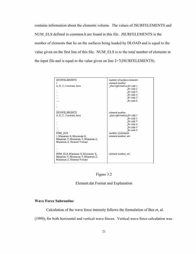
contains information about the elements volume. The values of JSURFELEMENTS and

NUM_ELS defined in common.h are found in this file. JSURFELEMENTS is the

number of elements that lie on the surfaces being loaded by DLOAD and is equal to the

value given on the first line of this file. NUM_ELS is to the total number of elements in

the input file and is equal to the value given on line 2+7(JSURFELEMENTS).

Figure 3.2

Element.dat Format and Explanation

Wave Force Subroutine

Calculation of the wave force intensity follows the formulation of Bea et, al.

(1999), for both horizontal and vertical wave forces. Vertical wave force calculation was

21

aided by Kerenyi’s technical notes (Kerenyi 2005). This formulation has been used

successfully in the oil industry for decades, giving results that match empirical

measurements of wave impact events. Furthermore, this method was selected so that the

loading could be varied as a function of time and position, which is not the case for the

other pressure based methods.

Surface Forces- Horizontal and Vertical

To determine the vertical and horizontal force intensities at surface integration

points, the size of the element face and the surface orientation are required. The

geometric information required for determination of element face area and orientation is

contained in the element.dat file. Because solid elements have six faces, one must first

determine which face the LIP lays in. The orientation of all elements faces is provided in

the element.dat file by specification of the equation the plane:

Ax + By + Cz + D = 0 (3.1)

A, B, C, and D are read from element.dat file. This information is then supplied to

DLOAD, where the subroutine runs through the plane information until the x, y, and z

coordinates of the LIPs satisfies Equation 3.1.

Once the correct plane has been identified, the vertical and horizontal components

of the surface forces are determined. The current implementation assumes that the

vertical direction is given by y, and that the motion of the wave is normal to the yz plane.

As such, all impact surfaces line parallel the z-axis. Thus the horizontal and vertical

components of the wave force are determined exclusively by a unit normal in the

direction (A,B). In DLOAD unit normal has the components (scale_x, scale_y).

22

One of the limitations of this approach is that the updated nodal coordinates are

not used to compute the vertical and horizontal wave force intensities, because

element.dat is based on the original coordinate positions given in the input file. This

limits the application to simulations with limited changes in surface orientation. As

stated above, Abaqus doe not provide access to the necessary information. One remedy

would be to update the element nodal positions and recomputed the element face

orientations.

DLOAD requires that the force be in units of FL-2, where F is a measurement of

force and L is a measurement of length. Equations 2.2 thru 2.4 were adjusted as follows:

F = scale _ x(0.5ρC u2 ) + scale _ y(0.5ρC w2 ) (3.2)s s s

Fd = scale _ x(0.5ρCdu2 ) (3.3)

Fl = scale _ y(0.5ρCl w2 ) (3.4)

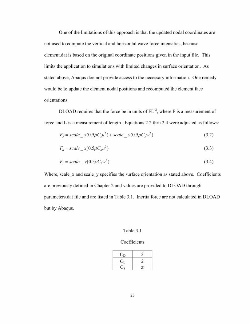
Where, scale_x and scale_y specifies the surface orientation as stated above. Coefficients

are previously defined in Chapter 2 and values are provided to DLOAD through

parameters.dat file and are listed in Table 3.1. Inertia force are not calculated in DLOAD

but by Abaqus.

Table 3.1

Coefficients

CD 2 CL 2 CS π

23

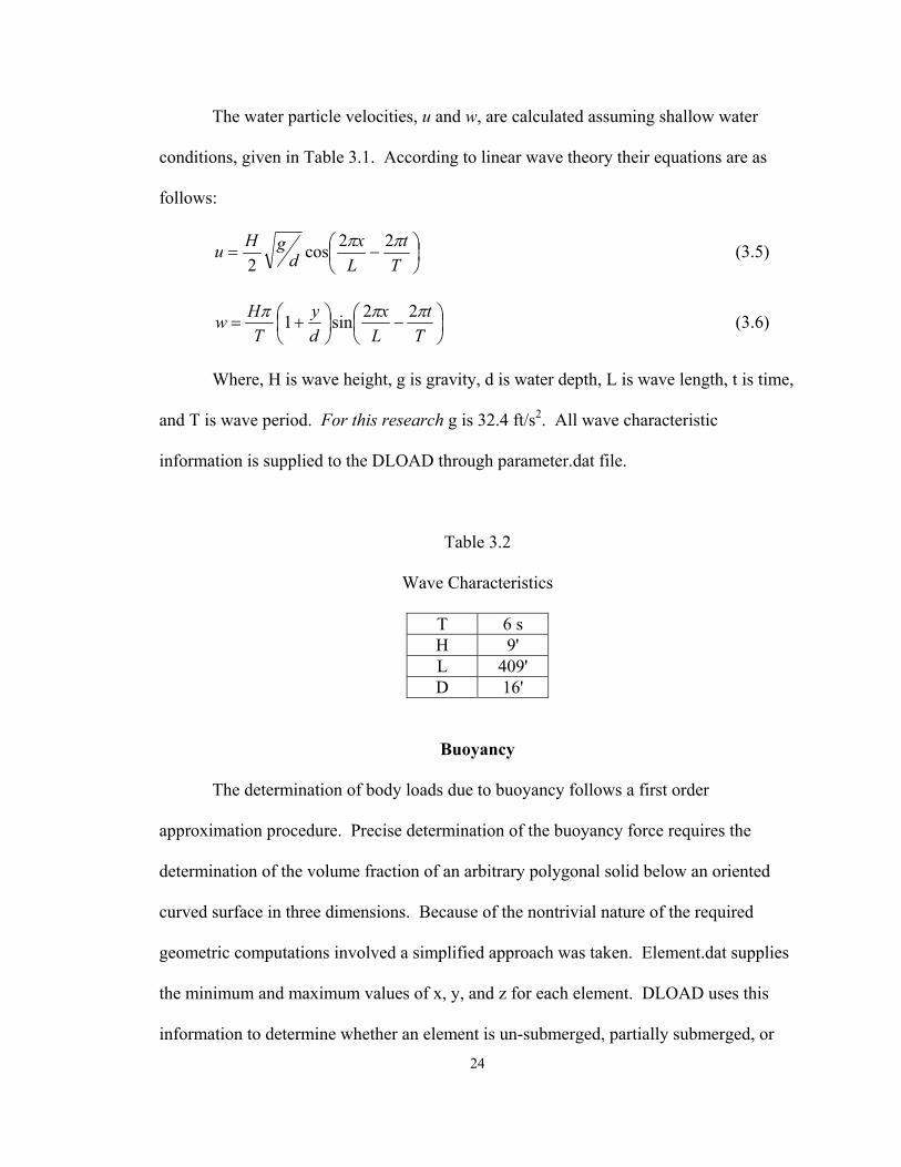
The water particle velocities, u and w, are calculated assuming shallow water

conditions, given in Table 3.1. According to linear wave theory their equations are as

follows:

H g ⎛ 2πx 2πt ⎞u = cos⎜ − ⎟ (3.5)d2 ⎝ L T ⎠

Hπ ⎛ y ⎞ ⎛ 2πx 2πt ⎞w = ⎜1 + ⎟ sin⎜ − ⎟ (3.6)T ⎝ d ⎠ ⎝ L T ⎠

Where, H is wave height, g is gravity, d is water depth, L is wave length, t is time,

and T is wave period. For this research g is 32.4 ft/s2. All wave characteristic

information is supplied to the DLOAD through parameter.dat file.

Table 3.2

Wave Characteristics

T 6 s H 9' L 409' D 16'

Buoyancy

The determination of body loads due to buoyancy follows a first order

approximation procedure. Precise determination of the buoyancy force requires the

determination of the volume fraction of an arbitrary polygonal solid below an oriented

curved surface in three dimensions. Because of the nontrivial nature of the required

geometric computations involved a simplified approach was taken. Element.dat supplies

the minimum and maximum values of x, y, and z for each element. DLOAD uses this

information to determine whether an element is un-submerged, partially submerged, or 24

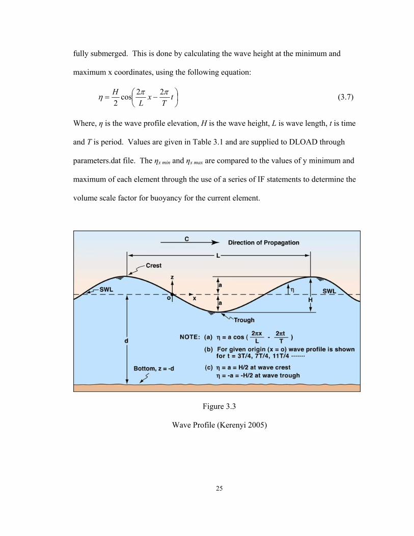
fully submerged. This is done by calculating the wave height at the minimum and

maximum x coordinates, using the following equation:

H ⎛ 2π 2π ⎞η = cos⎜ x − t ⎟ (3.7)2 ⎝ L T ⎠

Where, η is the wave profile elevation, H is the wave height, L is wave length, t is time

and T is period. Values are given in Table 3.1 and are supplied to DLOAD through

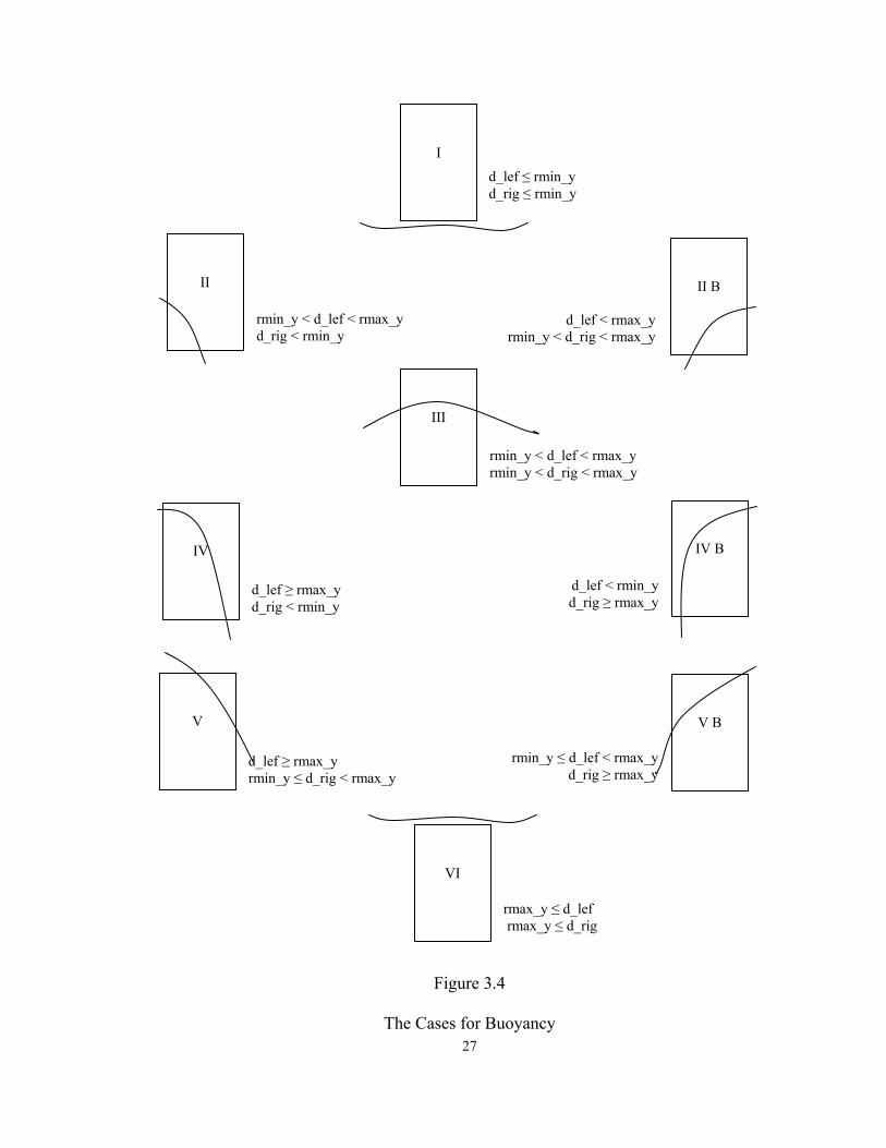
parameters.dat file. The ηx min and ηx max are compared to the values of y minimum and

maximum of each element through the use of a series of IF statements to determine the

volume scale factor for buoyancy for the current element.

Figure 3.3

Wave Profile (Kerenyi 2005)

25

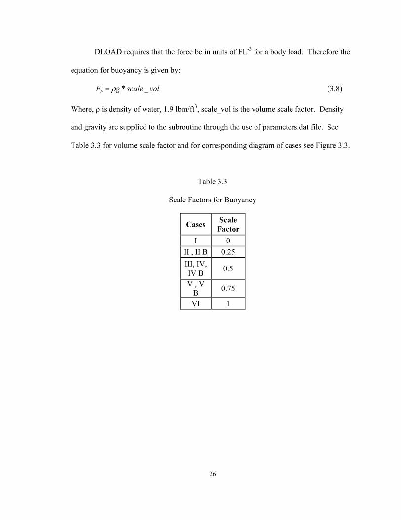
DLOAD requires that the force be in units of FL-3 for a body load. Therefore the

equation for buoyancy is given by:

Fb = ρg * scale _ vol (3.8)

Where, ρ is density of water, 1.9 lbm/ft3, scale_vol is the volume scale factor. Density

and gravity are supplied to the subroutine through the use of parameters.dat file. See

Table 3.3 for volume scale factor and for corresponding diagram of cases see Figure 3.3.

Table 3.3

Scale Factors for Buoyancy

Cases Scale Factor

I 0 II , II B 0.25 III, IV, IV B 0.5

V , V B 0.75

VI 1

26

I

d_lef ≤ rmin_y d_rig ≤ rmin_y

II II B

rmin_y < d_lef < rmax_y d_lef < rmax_y d_rig < rmin_y rmin_y < d_rig < rmax_y

III

rmin_y < d_lef < rmax_y rmin_y < d_rig < rmax_y

IV IV B

d_lef < rmin_y d_lef ≥ rmax_y d_rig ≥ rmax_y d_rig < rmin_y

rmin_y ≤ d_lef < rmax_y

V V B

d_lef ≥ rmax_y d_rig ≥ rmax_y rmin_y ≤ d_rig < rmax_y

VI

rmax_y ≤ d_lef rmax_y ≤ d_rig

Figure 3.4

The Cases for Buoyancy 27

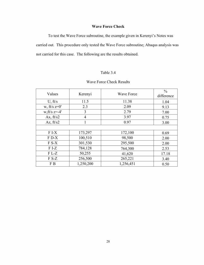
Wave Force Check

To test the Wave Force subroutine, the example given in Kerenyi’s Notes was

carried out. This procedure only tested the Wave Force subroutine; Abaqus analysis was

not carried for this case. The following are the results obtained.

Table 3.4

Wave Force Check Results

Values Kerenyi Wave Force %

difference U, ft/s 11.5 11.38 1.04

w, ft/s z=0' 2.3 2.09 9.13 w,ft/s z=-4' 3 2.79 7.00

Ax, ft/s2 4 3.97 0.75 Az, ft/s2 1 0.97 3.00

F I-X 173,297 172,100 0.69 F D-X 100,510 98,500 2.00 F S-X 301,530 295,500 2.00 F I-Z 784,128 764,300 2.53 F L-Z 50,255 41,620 17.18 F S-Z 256,500 265,221 3.40 F B 1,250,200 1,256,451 0.50

28

CHAPTER IV

NUMERICAL SIMULATION

Introduction

The program of choice is Abaqus, which was developed in 1978 by a group of

Brown Doctoral graduates. Abaqus is a general purpose finite element program which

has the capabilities of solving both static and dynamic problems, modeling large

displacement and contact problems. It also has a large library of elements and materials

available to the user.

Abaqus has two main methods of solving problems. The first is Abaqus/Standard

which solves a system of equation at each solution time increment using implicit

numerical integration. The second is Abaqus/Explicit which “marches a solution forward

through time in small time increments without solving a coupled system of equations at

each increment (Abaqus 2006).” For this research Abaqus/Standard will be used.

Abaqus uses steps so that a procedure can be solved using both static and dynamic

analysis. It also allows the user to prescribe loads, boundary conditions, and output

request for each step.

Abaqus has a built in feature, Aqua, that calculates wave loading. However due

to its makeup it was not able to be used for this research. “ABAQUS/Aqua contains

optional features that are specifically designed for the analysis of beam-like structures

installed underwater and subject to loading by water currents and wave action..” 29

Limitations are such that Abaqus/Aqua analysis “will calculate drag, buoyancy, and

inertia loading only for beam, pipe, elbow, truss, and certain rigid elements.” (Abaqus

2006)

Abaqus does not have built in units, except for rotation and angles. There the user

must take great care in making sure that all values are consistent. For this research,

English units will be used (feet and pounds).

Abaqus/CAE is a graphical interface where the user can specify all necessary

information. Abaqus must be supplied information about the geometry of an object. If a

model has more than one object, it must be told how the objects relate to each other- this

is done through the assembly module. The user must also specify a material model-

elastic, plastic, etc. More than one material model can be defined for an assembly of

objects. For an assembly, the interaction between the objects must be defined through

contact behavior. Along with interactions, the user must specify the boundary conditions.

Abaqus has a large library of different types of boundary conditions available to the user.

Loads can be applied to the objects as concentrated, distributed, and so on. As stated in

Chapter III, the loads can be supplied through the use of DLOAD. The user must also

specify the mesh density. The final step is to specify the analysis procedure and the

relevant parameters.

Model

Two models are examined in this research. The first is a simple block which is

used to assess the accuracy of the results by comparing numerical results with analytic

solutions. The second is that of a realistic bridge structure. The geometry of the model is

30

patterned after a typical section of the Biloxi Bay Bridge destroyed by Hurricane Katrina

in 2005.

Simple Block

The simple block example will be used purely as a way to check the validity of

Wave Force calculations and was used in debugging the interface between Abaqus and

the user subroutines, UEXTERNALDB and DLOAD.

Geometry

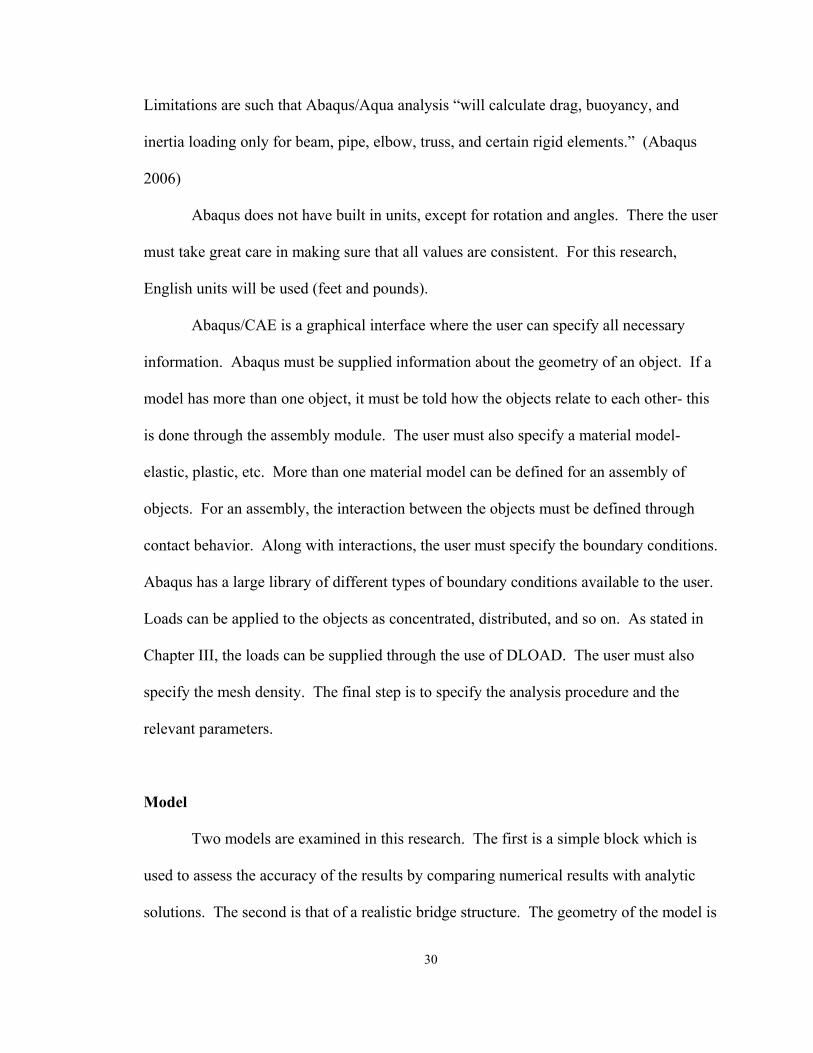
The block shown in Figure 4.1 was a length of 4’ and a height of 2’. The block is

made up of two C3D8R 8-node linear brick, three-dimensional solid elements. The

C3D8R element models stress/displacement and allows for reduced integration with an

hourglass control and six degrees of freedom at each node. The Hourglass control keeps

the elements from distorting “in such a way that the strains calculated at the integration

point are all zero, which, in turn, leads to uncontrolled distortion of the mesh (Abaqus

2006).”

31

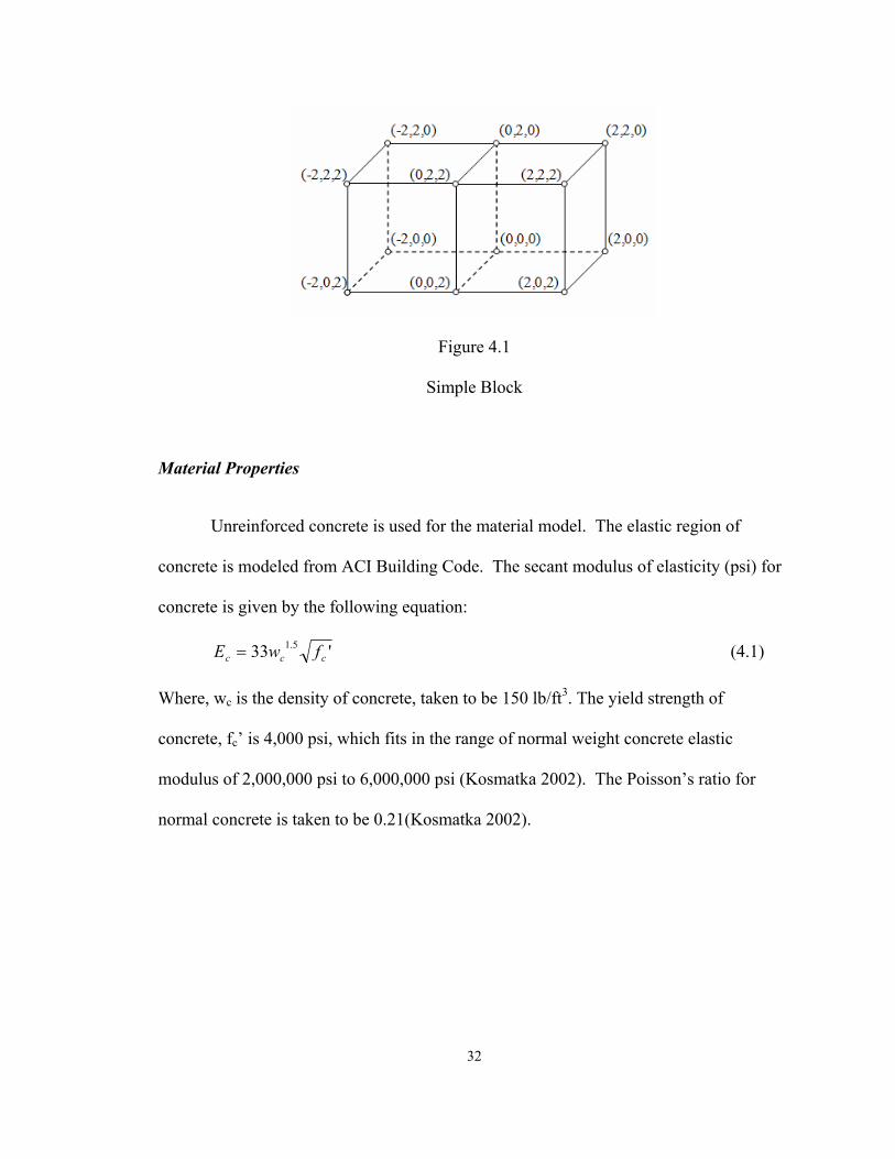
Figure 4.1

Simple Block

Material Properties

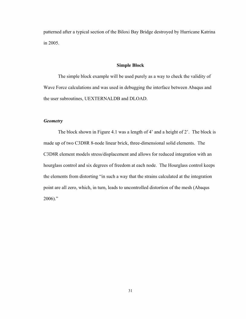
Unreinforced concrete is used for the material model. The elastic region of

concrete is modeled from ACI Building Code. The secant modulus of elasticity (psi) for

concrete is given by the following equation:

E = 33w 1.5 f ' (4.1)c c c

Where, wc is the density of concrete, taken to be 150 lb/ft3. The yield strength of

concrete, fc’ is 4,000 psi, which fits in the range of normal weight concrete elastic

modulus of 2,000,000 psi to 6,000,000 psi (Kosmatka 2002). The Poisson’s ratio for

normal concrete is taken to be 0.21(Kosmatka 2002).

32

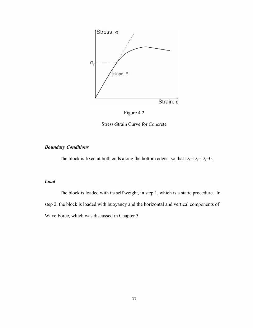
Figure 4.2

Stress-Strain Curve for Concrete

Boundary Conditions

The block is fixed at both ends along the bottom edges, so that Dx=Dy=Dz=0.

Load

The block is loaded with its self weight, in step 1, which is a static procedure. In

step 2, the block is loaded with buoyancy and the horizontal and vertical components of

Wave Force, which was discussed in Chapter 3.

33

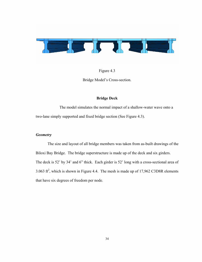
Figure 4.3

Bridge Model’s Cross-section.

Bridge Deck

The model simulates the normal impact of a shallow-water wave onto a

two-lane simply supported and fixed bridge section (See Figure 4.3).

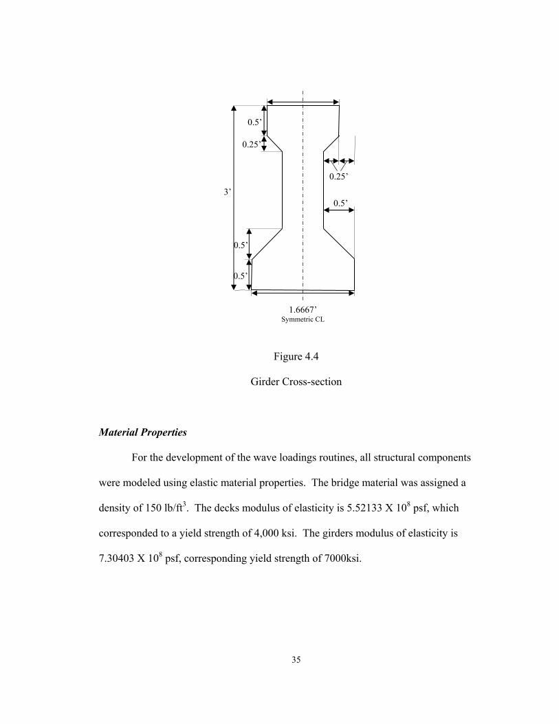
Geometry

The size and layout of all bridge members was taken from as-built drawings of the

Biloxi Bay Bridge. The bridge superstructure is made up of the deck and six girders.

The deck is 52’ by 34’ and 6” thick. Each girder is 52’ long with a cross-sectional area of

3.063 ft2, which is shown in Figure 4.4. The mesh is made up of 17,962 C3D8R elements

that have six degrees of freedom per node.

34

3’

1.1667’

0.5’

0.25’

0.5’

0.5’

0.5’

0.25’

1.6667’ Symmetric CL

Figure 4.4

Girder Cross-section

Material Properties

For the development of the wave loadings routines, all structural components

were modeled using elastic material properties. The bridge material was assigned a

density of 150 lb/ft3. The decks modulus of elasticity is 5.52133 X 108 psf, which

corresponded to a yield strength of 4,000 ksi. The girders modulus of elasticity is

7.30403 X 108 psf, corresponding yield strength of 7000ksi.

35

Support Boundary Conditions

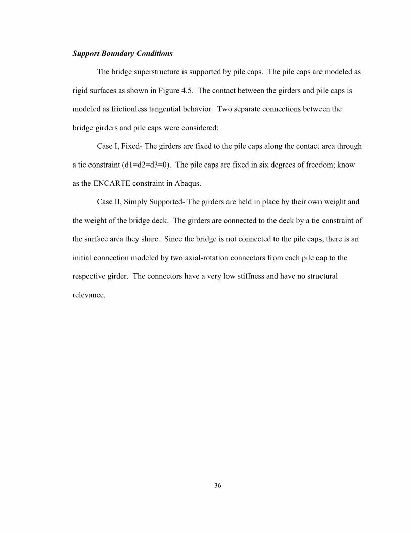
The bridge superstructure is supported by pile caps. The pile caps are modeled as

rigid surfaces as shown in Figure 4.5. The contact between the girders and pile caps is

modeled as frictionless tangential behavior. Two separate connections between the

bridge girders and pile caps were considered:

Case I, Fixed- The girders are fixed to the pile caps along the contact area through

a tie constraint (d1=d2=d3=0). The pile caps are fixed in six degrees of freedom; know

as the ENCARTE constraint in Abaqus.

Case II, Simply Supported- The girders are held in place by their own weight and

the weight of the bridge deck. The girders are connected to the deck by a tie constraint of

the surface area they share. Since the bridge is not connected to the pile caps, there is an

initial connection modeled by two axial-rotation connectors from each pile cap to the

respective girder. The connectors have a very low stiffness and have no structural

relevance.

36

Figure 4.5

Bridge Abaqus Solid Model

Load

Loading was applied in two steps. In step 1, the structure is loaded with gravity

and a static analysis procedure specified. In step 2, the superstructure of the bridge is

subjected to surface loads and buoyancy calculated by Wave Force subroutine. Note that

a clearance from bottom of bridge deck to SWE is 0’. From Douglass, it was shown that

the wave forces were greatest when the wave was not inundating the bridge but slapping

it (Douglass 2006).

37

Response of Structure

Simple Block

The simple block example was loaded with three different load cases: gravity

only, gravity plus buoyancy, and gravity, buoyancy, and surface loads. Since this

example is a Wave Force calculation check, the wave characteristics were those used in

the Kerenyi example, as shown in Table 4.1.

Table 4.1

Wave Characteristics for Simple Block

T 18 s H 16' L 409' D 16'

For the first case, simple block is loaded with only its self-weight. The maximum

displacement is approximately 0.007 inches at the mid-span. Using the equation for

maximum displacement (∆MAX) of a simply-supported beam with uniform distributed

load;

5wl 4

∆ = (4.2)MAX 384EI

Where w is the distributed load, in lb/in, l is the length of the beam in inches, E is the

elastic modulus in psi from equation 4.1, and I is the moment of inertia about the x-axis

in cubed inches. Using this equation a maximum displacement of 0.000 inches was

calculated.

38

For the second case, the simple block is loaded with both buoyancy and gravity.

The maximum displacement was calculated to be 0.004 inches. This agrees well with

expected result. Because the displacement for small displacements is linearly related to

the distributed load, the expected displacement of the submerged block is 0.007*(150-

62.4)/150=0.004. This shows that the buoyancy forces computed by the wave force were

correct. Comparing this value to the maximum displacement from gravity it is clear to

see that buoyancy is not great enough in this case to overcome gravity, due to the fact that

the block is not completely submerged.

For the third case, the simple block is loaded with gravity, buoyancy, and the

surface forces due to wave impact. The maximum displacement is 0.01 inches. From

this value it can be seen that the surface forces have some effect on the object.

After performing this example and looking at the displacements, the wave

characteristics were changed to those given in Table 3.1 to better model the conditions

for at the Biloxi Bay Bridge. For these characteristics, a maximum displacement of

0.00768 inches was calculated.

Bridge Deck

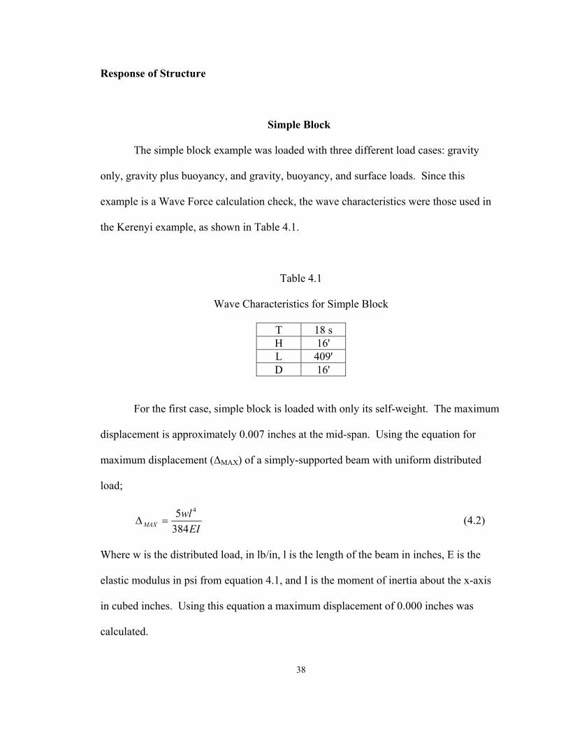
Case I- Fixed- The bridge section was loaded with the Wave Force subroutine

given the wave characteristics in Table 3.2 in Chapter III. A maximum deformation of

7/32” was observed at the seaward size of the mid span of the bridge deck, which is

shown in Figure 4.6.

39

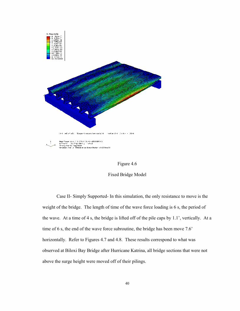
Figure 4.6

Fixed Bridge Model

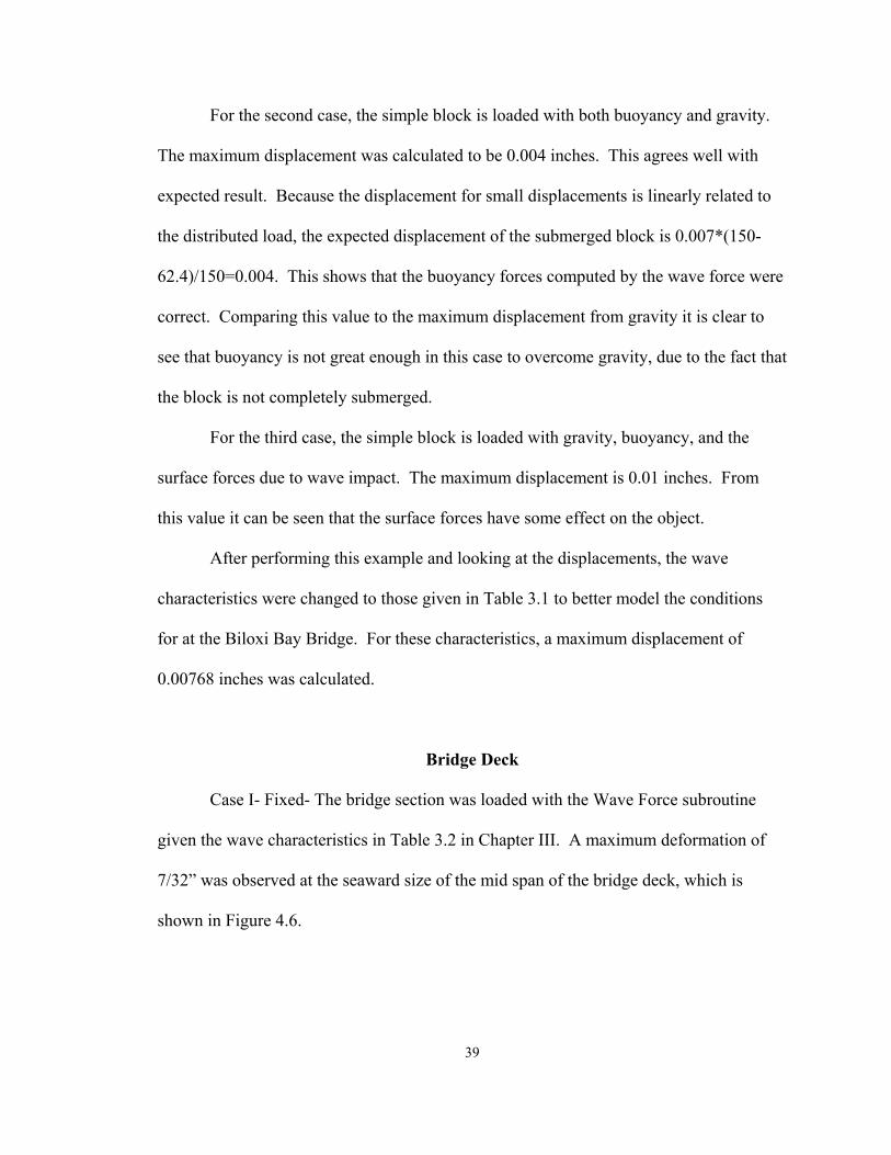
Case II- Simply Supported- In this simulation, the only resistance to move is the

weight of the bridge. The length of time of the wave force loading is 6 s, the period of

the wave. At a time of 4 s, the bridge is lifted off of the pile caps by 1.1’, vertically. At a

time of 6 s, the end of the wave force subroutine, the bridge has been move 7.6’

horizontally. Refer to Figures 4.7 and 4.8. These results correspond to what was

observed at Biloxi Bay Bridge after Hurricane Katrina, all bridge sections that were not

above the surge height were moved off of their pilings.

40

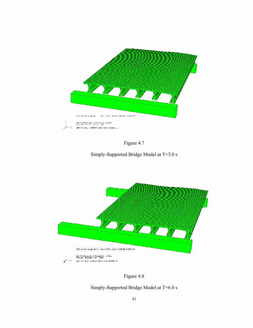
Figure 4.7

Simply-Supported Bridge Model at T=3.0 s

Figure 4.8

Simply-Supported Bridge Model at T=6.0 s

41

CHAPTER V

CONCLUSIONS

The destructive nature of storm surge on coastal structures makes the need to

examine the design procedures of essential structures critical. As a first step, the

development of methods to predict wave loads on complex structures was examined, and

computational routines were developed and implemented into the Abaqus finite element

code that application of time dependant, spatially varying wave forces to flexible

structures of arbitrary complexity.

This research did not address some areas of interest. For one, it did not address

energy dissipation of the wave from impacting the bridge. Moreover, computation of

wave forces did not account for movement of the structure. As such, wave forces were

computed using initial position of the bridge structure thus there may be cases in which

displaced geometry there would be no wave force, but forces are still applied. Once the

structure stops moving, there would be another impact force (Gullett 2008).

While the geometry of this model was based on typical bridge components taken

from design drawings, no effort was made to presentment the material behavior or the

inertial reinforcement of the bridge with precision. Changes for accurate representation

of the bridge structure would include representation of reinforcement, prestressing, and

material response.

42

The results that were obtained from fixing the bridge deck indicate that the bridge

would fall under wave force loading. The seaward most beam would be subjected to the

brunt of the wave, putting the seaward side into maximum compression and the leeward

side into maximum tension. The wave force effects would only be magnified when wind

and entrapped air were accounted for. Therefore, the best approach in designing bridges

for wave forces is to raise them above appropriate surge height.

43

REFERENCES

AASHTO. (2006). AASHTO LRFD Bridge Design Specifications, American Association of State Highway and Transportation Officials.

Abaqus, I. (2006). "Abaqus Version 6.6 PDF Documentation."

Bea, R. G., Xu, T., Stear, J., and Ramos, R. (1999). "Wave Forces on Decks of Offshore Platforms." Journal of Waterway, Port, Coastal, and Ocean Engineering, 125(May/June), 136-144.

Bergeron, A. (2007). "Contractor Ahead of Schedule On Biloxi Bay Bridge Erection."

Denson, K. (1981). "Final Report Pressures on Coastal Bridges Due to Normal Incidence Waves."

Douglass, S. L., Chen, Q., and Olsen, J. M. (2006). "Wave Forces on Bridge Decks." Office of Bridge Technology, Washington, DC.

Gullett, P. M. (2008). "(Personal Communication)."

Kerenyi, K. (2005). "Wave Forces on Bridge Decks." Federal Highway Administration, McLean, VA.

Kosmatka, S. H. (2002). "Design and Control of Concrete Mixtures." Portaland Cement Association, Skokie, Illinois.

McConnell, K. J., Allsop, N. W. H., Cuomo, G., and Cruickshank, I. C. (2003). "New Guidance for Wave Forces on Jetties in Exposed Locations." Proceedings of the Sixth Conference on coastal and Port Engineering Developing Countries, Colombo, Sri Lanka.

44

MDOT. (2006). "Gulf Coast Maps 2005 - Biloxi."

Morison, J. R., O'Brien, M. P., Johnson, J. W., and Schaaf, S. A. (1950). "The Force Exerted by Surface Waves on Piles." Petroleum Transactions, 189, 149-157.

O'Connor, J. (2005). " US 90 over Biloxi Bay Between Harrison and Jackson Counties, Mississippi."

Robertson, I. N., Riggs, H. R., Yim, S. C. S., and Young, Y. L. (2007). "Lessons from Hurricane Katrina Storm Surge on Bridges and Buildings." Journal of Waterway, Port, Coastal, and Ocean Engineering, 133(6), 463-483.

Wikipedia. (March 1, 2008). "Bridge."

Yim, S. C. (2005). "Modeling and Simulation of Tsunami and Storm Surge Hydrodynamic Loads on Coastal Bridge Structures."

45

APPENDIX A

USER SUBROUTINES

46

SOURCE.F

SUBROUTINE UEXTERNALDB(LOP,LRESTART,TIME,DTIME,KTSTEP,KINC)

INCLUDE 'ABA_PARAM.INC' CHARACTER*80 SNAME

INTEGER, PARAMETER :: IN_BR = 30INTEGER, PARAMETER :: SRMAX = 6INCLUDE 'COMMON.H'

OPEN (unit=IN_BR,1 file='/cavs/cmd/data1/users/maryd/element.dat',1 status='old')

READ(IN_BR,*) IDUM, IDUM

DO I=1,JSURFELEMENTSREAD(IN_BR,*) LIST_EL(I), PLANE_INFO(1,I),

PLANE_INFO(2,I),1 PLANE_INFO(3,I), PLANE_INFO(4,I),

PLANE_INFO(5,I),2 PLANE_INFO(6,I), PLANE_INFO(7,I),

PLANE_INFO(8,I),2 PLANE_INFO(9,I), PLANE_INFO(10,I),3 PLANE_INFO(11,I), PLANE_INFO(12,I),




PLANE_INFO(28,I),6 PLANE_INFO(29,I), PLANE_INFO(30,I)

CALL flush(6)END DO

READ(IN_BR,*) IDUM

DO I=1, NUM_ELSREAD(IN_BR,*) LIST_EL2(I), RMIN_X(I), RMAX_X(I),

RMIN_Y(I),1 RMAX_Y(I), RMIN_Z(I), RMAX_Z(I), VOL(I)

47

END DO

CLOSE(in_br)

RETURN END

SUBROUTINE DLOAD(F,KSTEP,KINC,TIME,NOEL,NPT,LAYER,KSPT,

1 COORDS,JLTYP,SNAME)

INCLUDE 'ABA_PARAM.INC'

DIMENSION TIME(2), COORDS(3)CHARACTER*80 SNAME

INCLUDE 'COMMON.H' IF (JLTYP.EQ.0) THENCALL SURFACEMAIN(COORDS,NOEL,TIME,F,NPT)

ELSE CALL BODYMAIN(COORDS,TIME,F,NOEL,NPT)

ENDIF

RETURN END

INCLUDE 'bodyforce.f'INCLUDE 'surfaceforce.f'

48

SURFACEFORCE.F

SUBROUTINE SURFACEMAIN(COORDS,NOEL,TIME,F,NPT)INCLUDE 'ABA_PARAM.INC'

DIMENSION COORDS(3), TIME(2)

INCLUDE 'COMMON.H' CALL PLANETEST(COORDS, NOEL, IPLANE)CALL WVPRTKIN(TIME,COORDS)CALL WVFORCE(COORDS,NOEL,TIME,F,NPT)

RETURN END

SUBROUTINE PLANETEST (COORDS, NOEL, IPLANE)


DIMENSION COORDS(3)CHARACTER*80 SNAME

INTEGER INDEX REAL*8 E1 PARAMETER(TOL=1E-2)

INCLUDE 'COMMON.H' DO I = 1, JSURFELEMENTSIF(NOEL .EQ. LIST_EL(I)) THENINDEX = I

END IF END DO

DO I = 1, 6J = (I - 1) * 5E1 =

PLANE_INFO(1+J,INDEX)*COORDS(1)+PLANE_INFO(2+J,INDEX)*1

COORDS(2)+PLANE_INFO(3+J,INDEX)*COORDS(3)+PLANE_INFO(4+J,INDEX)

IF (ABS(E1).LT. TOL) THENIPLANE = J GOTO 700

END IF END DO

700 CONTINUE 49

https://ABS(E1).LT

SCALE_X=ABS(PLANE_INFO(1+IPLANE,INDEX))SCALE_Y=ABS(PLANE_INFO(2+IPLANE,INDEX))AREA=PLANE_INFO(5+IPLANE,INDEX)

RETURN END

SUBROUTINE WVPRTKIN(TIME,COORDS)



REAL*8 THEAT, COST, SINT, PIOT, X, YINTEGER, PARAMETER :: K=21

INCLUDE 'COMMON.H'

OPEN (unit=K,file='/cavs/cmd/data1/users/maryd/parameters.dat',

1 status='old')

READ(K,*) DES, G, PI, D, H, WL, T, CD, CL, CS

CLOSE(K)

THETA=2*PI*((COORDS(1)/WL)-(TIME(1)/T) )COST=dCOS(THETA)SINT=dSIN(THETA)PIOT=PI/T

WVELX=0.5*H*dSQRT(G/D)*COSTWVELY=H*PIOT*(1+COORDS(2)/D)*SINT

RETURN END

SUBROUTINE WVFORCE(COORDS,NOEL,TIME,F,NPT)

INCLUDE 'ABA_PARAM.INC' DIMENSION TIME(2), COORDS(3)CHARACTER*80 SNAME

CHARACTER*80 SFILE INTEGER, PARAMETER :: fo_s=22

50

INCLUDE 'COMMON.H'

FDL=SCALE_X*(0.5*CD*DES*WVELX*WVELX)+1 SCALE_Y*(0.5*CL*DES*WVELY*WVELY)

FS=SCALE_X*(0.5*CS*DES*WVELX*WVELX)+1 SCALE_Y*(0.5*CS*DES*WVELY*WVELY)

F=FDL+FS

RETURN END

51

BODYFORCE.F

SUBROUTINE BODYMAIN(COORDS,TIME,F,NOEL,NPT)



CHARACTER*80 PFILE CHARACTER*80 BFILE INTEGER,PARAMETER :: fo_b=22REAL*8 DES, G, PI, D, H, WL, TINTEGER, PARAMETER :: L=21

REAL*8 WHL, WHRREAL*8 SCALE_VOL, LEG_X, LEG_Y, LEG_Z

INCLUDE 'COMMON.H'

PFILE='/cavs/cmd/data1/users/maryd/parameters.dat'OPEN (unit=L, file=PFILE, status='old')

READ(L,*) DES, G, PI, D, H, WL, T

CLOSE(L)

DO I = 1, NUM_ELSIF(NOEL .EQ. LIST_EL2(I)) THENINDEX = I

END IF END DO

WHL=0.5*H*DCOS((2*PI*RMIN_X(INDEX)/WL)-(2*PI*TIME(1)/T))

WHR=0.5*H*DCOS((2*PI*RMAX_X(INDEX)/WL)-(2*PI*TIME(1)/T))

IF (WHL>=0) THEND_LEF=CEILING(WHL)

ELSE D_LEF=FLOOR(WHL)

END IF

IF (WHR>=0) THEND_RIG=CEILING(WHR)

52

ELSE D_RIG=FLOOR(WHR)

END IF

IF (D_LEF<=RMIN_Y(INDEX) .AND. D_RIG<=RMIN_Y(INDEX))THEN

SCALE_VOL=0.00 ELSE IF (D_LEF>RMIN_Y(INDEX) .AND.

D_LEF<RMAX_Y(INDEX) .AND.1 D_RIG<RMIN_Y(INDEX)) THEN

SCALE_VOL=0.25 ELSE IF (D_LEF<RMIN_Y(INDEX) .AND.

D_RIG>RMIN_Y(INDEX) .AND.1 D_RIG<RMAX_Y(INDEX)) THEN

SCALE_VOL=0.25 ELSE IF (D_LEF>RMIN_Y(INDEX) .AND.

D_LEF<RMAX_Y(INDEX) .AND.1 D_RIG>RMIN_Y(INDEX) .AND. D_RIG<RMAX_Y(INDEX)) THEN

SCALE_VOL=0.50 ELSE IF (D_LEF>=RMAX_Y(INDEX) .AND.

D_RIG<RMIN_Y(INDEX)) THENSCALE_VOL=0.50

ELSE IF (D_LEF<RMIN_Y(INDEX) .AND.D_RIG>=RMAX_Y(INDEX)) THEN

SCALE_VOL=0.50 ELSE IF (D_LEF>=RMAX_Y(INDEX) .AND.

D_RIG>=RMIN_Y(INDEX) .AND.1 D_RIG<RMAX_Y(INDEX)) THEN

SCALE_VOL=0.75 ELSE IF (D_LEF>=RMIN_Y(INDEX) .AND.

D_LEF<RMAX_Y(INDEX) .AND.1 D_RIG>=RMAX_Y(INDEX)) THEN

SCALE_VOL=0.75 ELSE SCALE_VOL=1.00

END IF

F=DES*G*SCALE_VOL

RETURN END

53

https://SCALE_VOL=1.00









APPENDIX B

SIMPLE BLOCK EXAMPLE

54

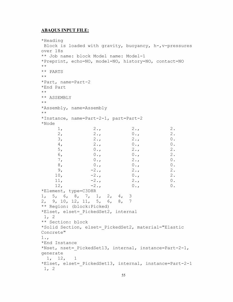
ABAQUS INPUT FILE:

*HeadingBlock is loaded with gravity, buoyancy, h-,v-pressuresover 18s ** Job name: block Model name: Model-1 *Preprint, echo=NO, model=NO, history=NO, contact=NO** ** PARTS ** *Part, name=Part-2*End Part ** ** ASSEMBLY ** *Assembly, name=Assembly** *Instance, name=Part-2-1, part=Part-2*Node

1, 2., 2., 2. 2, 2., 0., 2. 3, 2., 2., 0. 4, 2., 0., 0. 5, 0., 2., 2. 6, 0., 0., 2. 7, 0., 2., 0. 8, 0., 0., 0. 9, -2., 2., 2. 10, -2., 0., 2. 11, -2., 2., 0. 12, -2., 0., 0.

*Element, type=C3D8R1, 5, 6, 8, 7, 1, 2, 4, 3 2, 9, 10, 12, 11, 5, 6, 8, 7 ** Region: (block:Picked)*Elset, elset=_PickedSet2, internal1, 2** Section: block *Solid Section, elset=_PickedSet2, material="ElasticConcrete" 1.,*End Instance *Nset, nset=_PickedSet13, internal, instance=Part-2-1, generate

1, 12, 1 *Elset, elset=_PickedSet13, internal, instance=Part-2-11, 2

55

--------

*Nset, nset=_PickedSet15, internal, instance=Part-2-12, 4*Elset, elset=_PickedSet15, internal, instance=Part-2-11,*Nset, nset=_PickedSet16, internal, instance=Part-2-110, 12*Elset, elset=_PickedSet16, internal, instance=Part-2-12,*Nset, nset=_PickedSet20, internal, instance=Part-2-1, generate

1, 12, 1 *Elset, elset=_PickedSet20, internal, instance=Part-2-11, 2*Elset, elset=__PickedSurf22_S4, internal, instance=Part-2-1 1, 2*Surface, type=ELEMENT, name=_PickedSurf22, internal__PickedSurf22_S4, S4*Elset, elset=__PickedSurf23_S1, internal, instance=Part-2-1 2,*Surface, type=ELEMENT, name=_PickedSurf23, internal__PickedSurf23_S1, S1*End Assembly** ** MATERIALS ** *Material, name="Elastic Concrete"*Density150.,*Elastic 5.52096e+08, 0.21** ** BOUNDARY CONDITIONS ** ** Name: BC-1 Type: Displacement/Rotation*Boundary_PickedSet16, 1, 1_PickedSet16, 2, 2_PickedSet16, 6, 6** Name: BC-2 Type: Displacement/Rotation*Boundary_PickedSet15, 2, 2** --------------------------------------------------------

** ** STEP: load

56

** *Step, name=load*Dynamic,alpha=-0.05,direct,nohaf2.,6.,** ** LOADS ** ** Name: Buoyancy Type: Body force*Dload _PickedSet20, BYNU, 1.** Name: Gravity Type: Gravity*Dload _PickedSet13, GRAV, 1., 0., -1., 0.** Name: Horizontal Type: Pressure*Dsload _PickedSurf23, PNU, 1.** Name: Vertical Type: Pressure*Dsload _PickedSurf22, PNU, 1.** ** OUTPUT REQUESTS** *Restart, write, frequency=1** ** FIELD OUTPUT: F-Output-1** *Output, field, variable=PRESELECT, frequency=1** ** HISTORY OUTPUT: H-Output-1** *Output, history, variable=PRESELECT*El Print, freq=999999*Node Print, freq=999999*End Step

COMMON.H FILE:

PARAMETER(JSURFELEMENTS=2)PARAMETER(NUM_ELS=2)COMMON /SURF_ORIENT/1 LIST_EL(JSURFELEMENTS),1 PLANE_INFO(30,JSURFELEMENTS),1 LIST_EL2(NUM_ELS),1 RMIN_X(NUM_ELS), RMIN_Y(NUM_ELS),

RMIN_Z(NUM_ELS), 57

1 RMAX_X(NUM_ELS), RMAX_Y(NUM_ELS),RMAX_Z(NUM_ELS),

1 VOL(NUM_ELS),1 SCALE_X, SCALE_Y, AREA, WVELX, WVELY,1 DES, G, PI, D, H, WL, T, A1, A2, CD, CL, CS

PARAMETERS.DAT FILE:

1.900000E+00 32.400000E+00 3.141593E+00 16.000000E+00 16.000000E+00 409.000000E+00 18.000000E+00 1.000000E+00 1.000000E+00 1.000000E+00 1.000000E+00 1.000000E+00

ELEMENT.DAT FILE:

2 11 1

0.100000E+01 0.000000E+00 0.000000E+00 0.000000E+00 0.400000E+01

0.100000E+01 0.000000E+00 0.000000E+00 -0.200000E+01 0.400000E+01

0.000000E+00 -0.100000E+01 0.000000E+00 0.000000E+00 0.400000E+01

0.000000E+00 -0.100000E+01 0.000000E+00 0.200000E+01 0.400000E+01

0.000000E+00 0.000000E+00 0.100000E+01 -0.200000E+01 0.400000E+01

0.000000E+00 0.000000E+00 0.100000E+01 0.000000E+00 0.400000E+01

2 0.100000E+01 0.000000E+00 0.000000E+00 0.200000E+01

0.400000E+01 0.100000E+01 0.000000E+00 0.000000E+00 0.000000E+00

0.400000E+01 0.000000E+00 -0.100000E+01 0.000000E+00 0.000000E+00

0.400000E+01 0.000000E+00 -0.100000E+01 0.000000E+00 0.200000E+01

0.400000E+01 0.000000E+00 0.000000E+00 0.100000E+01 -0.200000E+01

0.400000E+01 0.000000E+00 0.000000E+00 0.100000E+01 0.000000E+00

0.400000E+01 58

2 1 0.0000E+00 0.2000E+01 0.0000E+00 0.2000E+01

0.0000E+00 0.2000E+01 0.8000E+01 2 -0.2000E+01 0.0000E+00 0.0000E+00 0.2000E+01

0.0000E+00 0.2000E+01 0.8000E+01

59

APPENDIX C

FIXED BRIDGE EXAMPLE

60

ABAQUS INPUT FILE:

Not included (1000+ pages), on CD.

COMMON.H FILE:


RMIN_Z(NUM_ELS),1 RMAX_X(NUM_ELS), RMAX_Y(NUM_ELS),

RMAX_Z(NUM_ELS),1 VOL(NUM_ELS),1 SCALE_X, SCALE_Y, AREA, WVELX, WVELY,1 DES, G, PI, D, H, WL, T, A1, A2, CD, CL, CS

PARMETERS.DAT FILE:

1.900000E+00 32.400000E+00 3.141593E+00 16.000000E+00 9.000000E+00 409.000000E+00 6.000000E+00 2.000000E+00 2.000000E+00 3.141593E+00

ELEMENT.DAT FILE:

Not included (2000+pages), on CD.

61

APPENDIX D

SIMPLY-SUPPORTED BRIDGE EXAMPLE

62

ABAQUS INPUT FILE:

Not included (1000+ pages), on CD

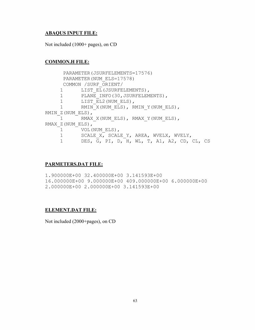
COMMON.H FILE:


RMIN_Z(NUM_ELS),1 RMAX_X(NUM_ELS), RMAX_Y(NUM_ELS),

RMAX_Z(NUM_ELS),1 VOL(NUM_ELS),1 SCALE_X, SCALE_Y, AREA, WVELX, WVELY,1 DES, G, PI, D, H, WL, T, A1, A2, CD, CL, CS

PARMETERS.DAT FILE:

1.900000E+00 32.400000E+00 3.141593E+00 16.000000E+00 9.000000E+00 409.000000E+00 6.000000E+00 2.000000E+00 2.000000E+00 3.141593E+00

ELEMENT.DAT FILE:

Not included (2000+pages), on CD

63

APPENDIX E

ABAQUS TUTORIAL

64

1. Open Terminal

2. Type Command: swsetup abaqus-6.5

3. Type Command: abaqus cae

4. In “Start Session” window, click on “Create Model Database”.

In Module: Part,

1. Click “Create Part”.

2. In “Create Part” window,

a. Name: type Beam

b. Modeling Space: 3D

c. Shape: Solid

d. Type: Extrusion

e. Approximate size: type 9.

f. Click on “Continue…”.

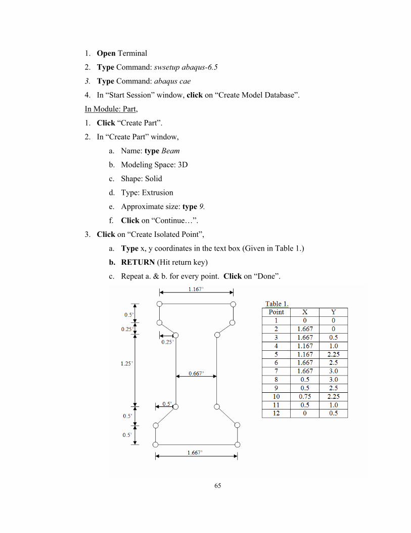
3. Click on “Create Isolated Point”,

a. Type x, y coordinates in the text box (Given in Table 1.)

b. RETURN (Hit return key)

c. Repeat a. & b. for every point. Click on “Done”.

65

4. Click on “Create Lines: Connected”, select the first point, then second until all

points are connected with a single line.

5. Click on “Done” Twice

6. In “Edit Base Extrusion”, choose

a. Type: Blind

b. Depth: type 16’

7. Click on “Ok”.

In Module: Property,

1. Click on “Create Material”

2. Name: type Concrete

3. Click on “General”,

a. Click on “Density”

b. Leave “Use temperature-dependent data” unchecked.

c. Leave “Number of field variables:” to O.

d. For “Mass Density”, Type 150 (lbs/ft2).

4. Click on “Mechanical”

a. Click on “Elasticity”

b. Click on “Elastic”

c. Leave Type: Isotropic

d. Leave “Use temperature-dependent data” unchecked

e. Leave “Number of field variables:” to O

f. Leave “Moduli time scale (for viscoelasticity):” long-term

g. For “Young’s Modulus”: Type 552096.E3 (lbs/ft2).

h. For “Poisson’s Ratio”: Type 0.21

i. Click on “OK”.

5. Click on “Create Section”,

a. Name: type Cross-Section

b. Category: Solid

c. Type: Homogeneous

d. Click on “Continue…”

6. In “Edit Section” window,

66

https://552096.E3

a. Select Concrete for “Material”.

b. Type 1 for “Plane stress/strain thickness”.

c. Click on “OK”

7. Click on “Assign Section”, notice in prompt area it says to “Select the regions to

be assigned a section”, click on the beam.….

8. Click on “Done”.

9. Click on “Ok”.

In Module: Assembly,

1. Click on “Instance Part”

2. Select Beam

3. Click on “OK” (notice that the beam is now blue this means the part is now a

instance)

In Module: Step,

1. Click on “Create Step”,

a. Name: Type Gravity

b. Insert new step after: Initial

c. Procedure type: General

d. Select “Static, General”

e. Click on “Continue…”

4. In “Edit Step” window, for description type Beam is loaded with it's own weight.

5. Click on “OK”.

6. Click on “Create Step”,

a. Name: Type Load

b. Insert new step after: Initial

c. Procedure type: General

d. Select “Static, General”


7. In “Edit Step” window, for description type Pressure is applied to bottom surface

of beam.


67

In Module: Load,

1. Click on “Create Boundary Condition”

2. In “Create Boundary Condition” window,

a. Name: type Pinned.

b. Step: select Initial

c. Category: Mechanical

d. Types for Selected Step: Displacement/Rotation


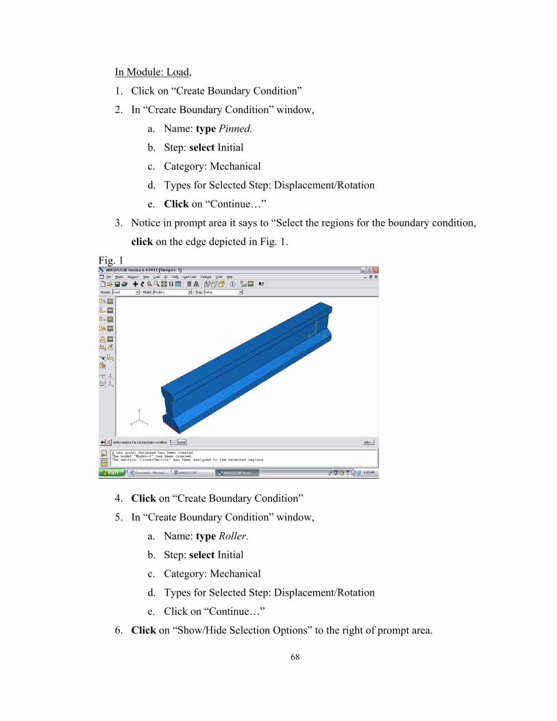
3. Notice in prompt area it says to “Select the regions for the boundary condition,

click on the edge depicted in Fig. 1.

Fig. 1

4. Click on “Create Boundary Condition”

5. In “Create Boundary Condition” window,

a. Name: type Roller.

b. Step: select Initial


d. Types for Selected Step: Displacement/Rotation


6. Click on “Show/Hide Selection Options” to the right of prompt area.

68

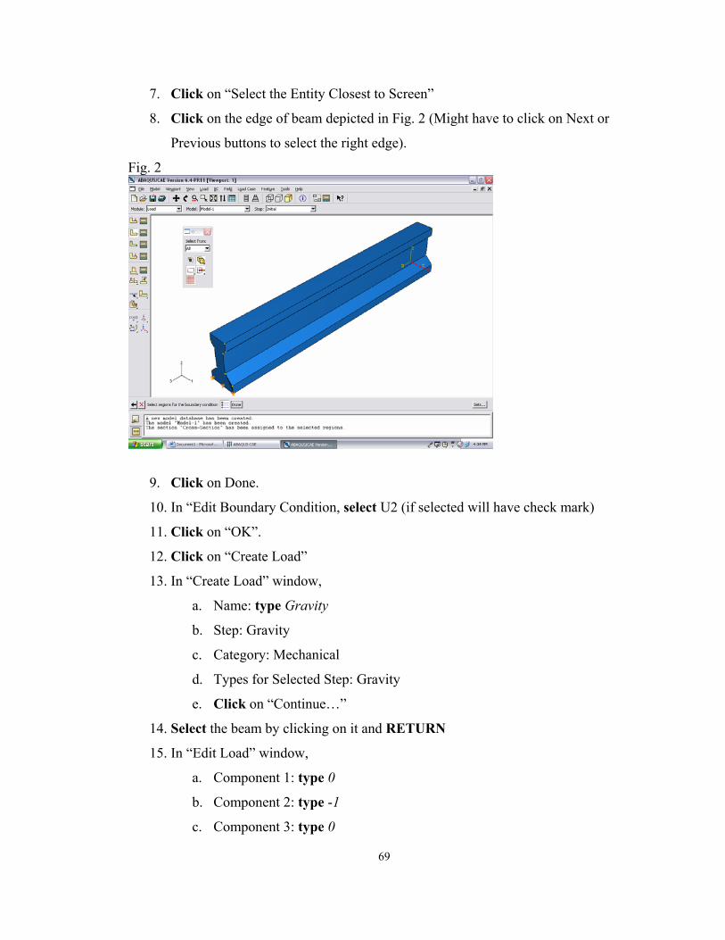
7. Click on “Select the Entity Closest to Screen”

8. Click on the edge of beam depicted in Fig. 2 (Might have to click on Next or

Previous buttons to select the right edge).

Fig. 2

9. Click on Done.

10. In “Edit Boundary Condition, select U2 (if selected will have check mark)


12. Click on “Create Load”

13. In “Create Load” window,

a. Name: type Gravity

b. Step: Gravity


d. Types for Selected Step: Gravity


14. Select the beam by clicking on it and RETURN

15. In “Edit Load” window,

a. Component 1: type 0

b. Component 2: type -1

c. Component 3: type 0

69

d. Amplitude: (Ramp)

e. Click on “OK”. (Yellow arrows pointing downward should appear)

16. Click on “Create Load”

17. In “Create Load” window,

a. Name: type Pressure

b. Step: Load


d. Types for Selected Step: Pressure


18. Click on “Show/Hide Selection Options” to the right of prompt area.

19. Click on “Select the Entity Closest to Screen”

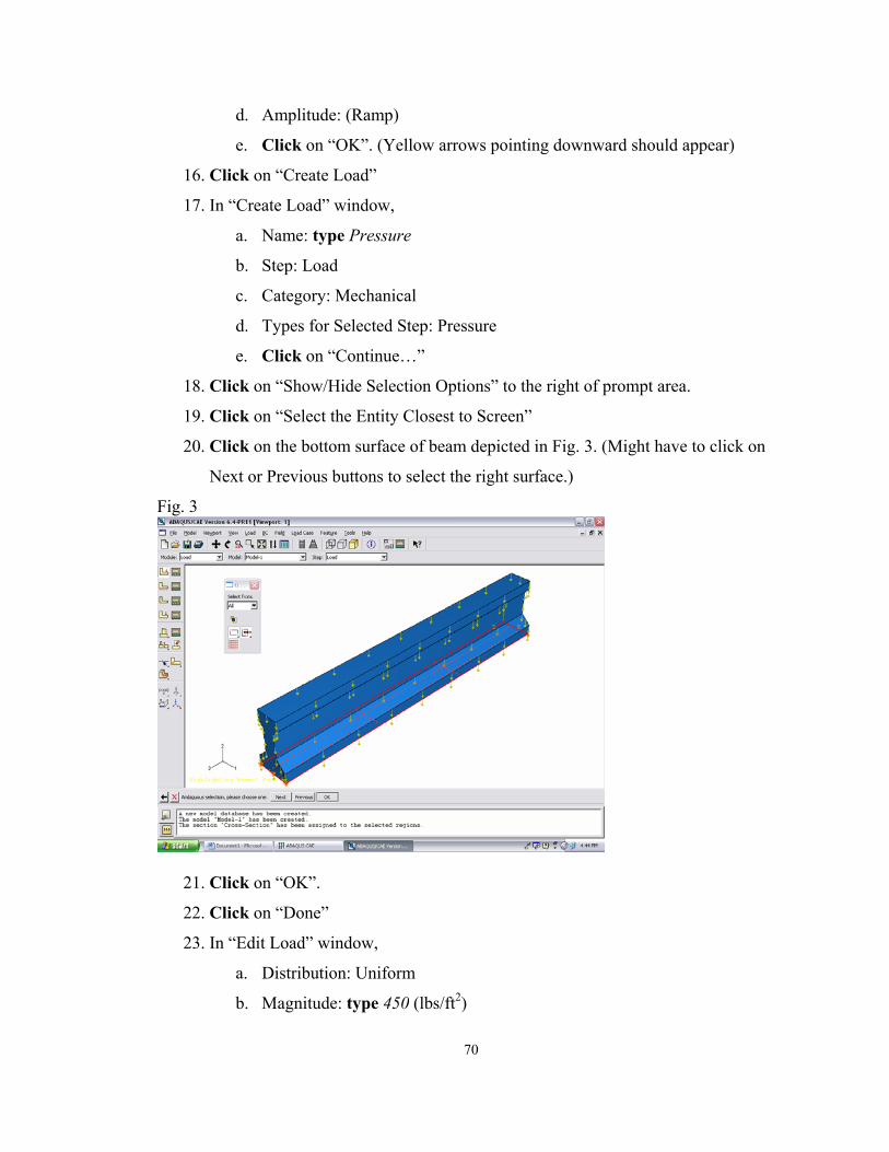
20. Click on the bottom surface of beam depicted in Fig. 3. (Might have to click on

Next or Previous buttons to select the right surface.)

Fig. 3


22. Click on “Done”

23. In “Edit Load” window,

a. Distribution: Uniform

b. Magnitude: type 450 (lbs/ft2)

70

c. Amplitude: (Ramp)

d. Click on “OK”

In Module: Mesh

Notice that beam is now yellow, therefore we must partition beam into smaller parts.

1. Click on “Tools” (in the main menu bar).

2. Click on “Datum”

3. In “Create Datum” window,

a. Select “Point”

b. Select “Offset from point”

c. Click on “Apply”

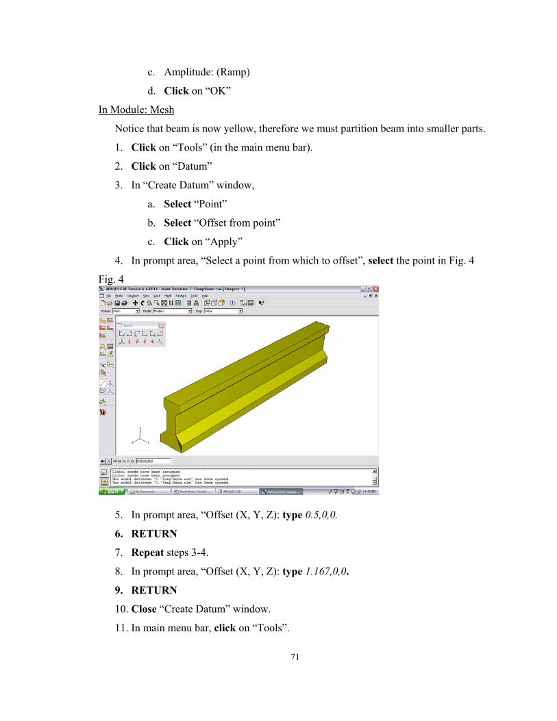
4. In prompt area, “Select a point from which to offset”, select the point in Fig. 4

Fig. 4

5. In prompt area, “Offset (X, Y, Z): type 0.5,0,0.

6. RETURN

7. Repeat steps 3-4.

8. In prompt area, “Offset (X, Y, Z): type 1.167,0,0.

9. RETURN

10. Close “Create Datum” window.

11. In main menu bar, click on “Tools”.

71

12. Click on “Partition”.

13. In “Create Partition” window,

a. Select “cell” as “Type”

b. Select “Define cutting plane” as “Method”

c. Click on “Apply”.

d. In prompt area, “How do you want to specify the plane?”, select 3 Points

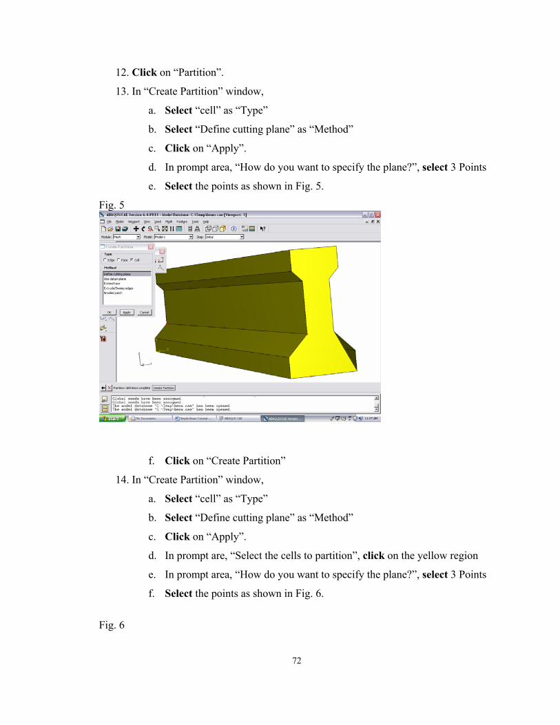
e. Select the points as shown in Fig. 5.

Fig. 5

f. Click on “Create Partition”

14. In “Create Partition” window,

a. Select “cell” as “Type”

b. Select “Define cutting plane” as “Method”

c. Click on “Apply”.

d. In prompt are, “Select the cells to partition”, click on the yellow region

e. In prompt area, “How do you want to specify the plane?”, select 3 Points

f. Select the points as shown in Fig. 6.

Fig. 6

72

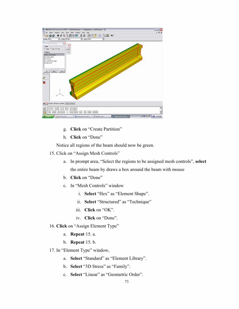
g. Click on “Create Partition”

h. Click on “Done”

Notice all regions of the beam should now be green.

15. Click on “Assign Mesh Controls”

a. In prompt area, “Select the regions to be assigned mesh controls”, select

the entire beam by draws a box around the beam with mouse

b. Click on “Done”

c. In “Mesh Controls” window

i. Select “Hex” as “Element Shape”.

ii. Select “Structured” as “Technique”

iii. Click on “OK”.

iv. Click on “Done”.

16. Click on “Assign Element Type”

a. Repeat 15. a.

b. Repeat 15. b.

17. In “Element Type” window,

a. Select “Standard” as “Element Library”.

b. Select “3D Stress” as “Family”.

c. Select “Linear” as “Geometric Order”. 73

d. Click on “Ok”

18. Click on “Seed Part Instance”

19. In prompt area, type 1 for “Global element size (approximate):”

20. RETURN

21. Click on “Mesh Part Instance”

22. Click on “Yes”.

23. Click on “Auto Fix View” icon to adjust view.

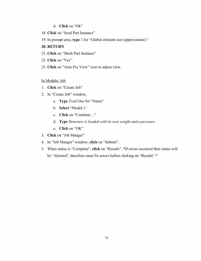
In Module: Job

1. Click on “Create Job”

2. In “Create Job” window,

a. Type Trail One for “Name”.

b. Select “Model-1’.

c. Click on “Continue…”

d. Type Structure is loaded with its own weight and a pressure.

e. Click on “OK”

3. Click on “Job Manger”

4. In “Job Manger” window, click on “Submit”.

5. When status is “Complete”, click on “Results”. *If errors occurred then status will

be “Aborted”, therefore must fix errors before clicking on “Results”.*

74

APPENDIX F

ABAQUS/WAVE FORCE STEPS

75

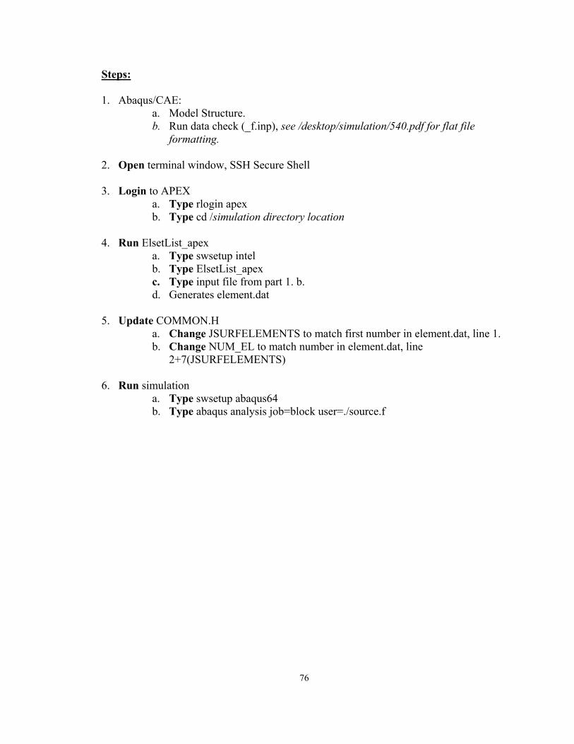
Steps:

1. Abaqus/CAE: a. Model Structure. b. Run data check (_f.inp), see /desktop/simulation/540.pdf for flat file

formatting.

2. Open terminal window, SSH Secure Shell

3. Login to APEX a. Type rlogin apex b. Type cd /simulation directory location

4. Run ElsetList_apex a. Type swsetup intel b. Type ElsetList_apex c. Type input file from part 1. b. d. Generates element.dat

5. Update COMMON.H a. Change JSURFELEMENTS to match first number in element.dat, line 1. b. Change NUM_EL to match number in element.dat, line

2+7(JSURFELEMENTS)

6. Run simulation a. Type swsetup abaqus64 b. Type abaqus analysis job=block user=./source.f

76

Documents

WAVE FORCES ON BRIDGES Mary-Margaret Dickey