Wave-induced stress and breaking of sea ice in a coupled

Wave-induced stress and breaking of sea ice in a coupledhydrodynamic–discrete-element wave–ice modelAgnieszka Herman1

1Institute of Oceanography, University of Gdansk, Poland

Correspondence to: A. Herman ([email protected])

Abstract. In this paper, a coupled sea ice–wave model is developed and used to analyze the variability of wave-induced stress

and breaking in sea ice. The sea ice module is a discrete-element bonded-particle model, in which ice is represented as cuboid

“grains” floating on the water surface that can be connected to their neighbors by elastic “joints”. The joints may break if

instantaneous stresses acting on them exceed their strength. The wave part is based on an open-source version of the Non-

Hydrostatic WAVE model (NHWAVE). The two parts are coupled with proper boundary conditions for pressure and velocity,5

exchanged at every time step. In the present version, the model operates in two dimensions (one vertical and one horizontal)

and is suitable for simulating compact ice in which heave and pitch motion dominates over surge. In a series of simulations

with varying sea ice properties and incoming wavelength it is shown that wave-induced stress reaches maximum values at

a certain distance from the ice edge. The value of maximum stress depends on both ice properties and characteristics of

incoming waves, but, crucially for ice breaking, the location at which the maximum occurs does not change with the incoming10

wavelength. Consequently, both regular and random (Jonswap spectrum) waves break the ice into floes with almost identical

sizes. The width of the zone of broken ice depends on ice strength and wave attenuation rates in the ice.

1 Introduction

Interactions between sea ice and waves are a defining characteristic of the marginal ice zone (MIZ), loosely defined as a region

of the ice cover adjacent to the ice edge and directly influenced by the neighboring open ocean. In recent years, as the sea ice15

extent in polar and subpolar regions decreases and thick, multi-year ice is replaced with thinner, weaker seasonal ice, conditions

typical for MIZ (ice concentration lower than 90%, small floe sizes, patchy distribution of floes on the sea surface, etc.) tend

to occur over larger and larger areas. There is a growing observational and modeling evidence that wave–ice interactions

play an important role in the observed expansion of MIZ and negative trends in sea ice extent (see, e.g., Asplin et al., 2012,

2014; Thomson and Rogers, 2014; Thomson et al., 2016). Thin, fragmented sea ice is susceptible to further breaking and,20

depending on ambient weather and oceanic conditions, melting, which facilitates faster ice drift, decrease in ice concentration,

increase in wind fetch, and thus creates more favorable conditions for wave propagation and generation, leading to still stronger

fragmentation. These – and many other – feedbacks show that it is crucial to include (the effects of) wave–ice interactions in

numerical ocean–sea ice–atmosphere models in order to be able to reliably reproduce the observed processes and forecast future

changes on both synoptic and climate scales. Parameterizations of wave–ice interactions for large-scale, continuum models are25

1

The Cryosphere Discuss., doi:10.5194/tc-2017-95, 2017Manuscript under review for journal The CryosphereDiscussion started: 29 May 2017c© Author(s) 2017. CC-BY 3.0 License.

crucial for further development of those models. However, although appreciable effort has been made in that direction in recent

years (Dumont et al., 2011; Doble and Bidlot, 2013; Squire et al., 2013; Williams et al., 2013, 2017), our understanding of

many aspects of wave–ice interactions is still too limited to allow formulating such parameterizations, especially those suitable

for a wide range of conditions. Strong fragmentation of the ice into many small floes, and highly energetic environment due

to the presence of waves make the MIZ a very difficult, demanding location for field work. Due to low temporal resolution of5

satellite data in polar regions, they provide only snapshots of sea ice conditions, making it difficult or impossible to infer details

of processes acting on time scales comparable with a typical wave period. Therefore, the amount of observational data from the

MIZ, necessary for validation of numerical models, remains very limited. Consequently, many seemingly basic processes are

only poorly understood. For example, the functional form describing the rate of change of wave height with distance from the

ice edge is far from established. Whereas most observations and models suggest exponential attenuation of waves propagating10

into the MIZ (e.g., Squire et al., 2009; Vaughan et al., 2009; Dumont et al., 2011), recent observations by Kohout et al. (2014)

provide a different picture. During a storm event in the Southern Ocean, they observed exponential decay of wave height with

distance for small waves, but much slower, approximately linear decay for waves exceeding 3 m in height. This led to the ice

break-up hundreds of kilometers from the open ocean. Kohout et al. (2014) showed also the existence of strong correlation

between the trends in the sea ice extent and significant wave height at various sections of the Southern Ocean during both ice15

growth and melting seasons – providing yet another example of how important sea ice–wave interactions are on larger scales.

Review papers by Squire et al. (1995) and Squire (2007, 2011) provide a good overview of the state-of-the-art research

related to wave–ice interactions. Problems studied in this context include, but are not limited to: wave propagation, attenuation

and scattering by various ice types, e.g., continuous ice sheets, broken compact ice, (groups of) individual ice floes, and

inhomogeneities like pressure ridges, cracks etc.; motion of ice floes (and other floating objects, including very large floating20

structures) on waves and wave-induced floe collisions; sea ice breaking by waves. Considering relatively rich literature on wave

propagation in sea ice and wave-induced motion of ice floes/sheets (see, e.g., Squire, 1983; Liu and Mollo-Christensen, 1988;

Shen and Ackley, 1991; Meylan and Squire, 1994; Meylan, 2002; Wang and Shen, 2011; Montiel et al., 2012, 2016; Sutherland

and Rabault, 2016, and references there, as this list is by far not complete), the number of studies on sea ice breaking by waves

is remarkably limited and – as Squire et al. (1995) aptly put it – they are to a large degree based on “anecdotal evidence”. In25

a series of papers published in 1980s, V. Squire analyzed wave propagation in continuous, land-fast ice and basic mechanisms

of wave-induced ice breaking (see, e.g., Squire, 1984a, b). In their review paper, Squire et al. (1995) describe qualitatively the

process of breaking of land-fast ice by swell waves, in which elongated, parallel strips of ice are progressively separated from

the initially continuous ice sheet. They write that “the width of the strips, and hence the diameter of the floes created by the

process, is remarkably consistent and appears in the sparse evidence available to be rather insensitive to the spectral structure30

of the sea, but highly dependent on ice thickness.” Consistently, their modeling results showed that the location of maximum

flexural strain in the ice relative to the ice edge depends mainly on ice thickness rather than wave period. Notwithstanding these

conclusions, a close relationship between the incoming wavelength and floe sizes produced by breaking is usually assumed, as

for example in the above-mentioned parameterizations by Williams et al. (2013) and others.

2


Since the pioneering works described above, few studies have been devoted specifically to the analysis of sea ice breaking by35

waves. In a modeling study of ice motion on waves, Meylan and Squire (1994) analyzed flexural strain variability in ice floes

of different sizes and thicknesses. Langhorne et al. (1998) analyzed experimentally and numerically the fatigue behavior of

first-year sea ice subject to repeated bending stress and demonstrated that the time history of strain acting on the ice is crucial

for predicting its breaking. In a subsequent work, Langhorne et al. (2001) extended their earlier work to estimate lifetime of

landfast ice subject to waves with given characteristics. Based on ship observations of ice breaking during a strong-wave event5

in the Barents Sea, Collins et al. (2015) analyzed the role of nonlinear wave processes and the resulting strong modulation

of wave amplitude in ice breaking, in accordance with much earlier observations and theoretical results of Liu and Mollo-

Christensen (1988). Using results of Squire et al. (2009) and Vaughan et al. (2009) to estimate the evolution of wave energy

spectra in the Arctic sea ice, Vaughan and Squire (2011) estimated ice breaking probabilities in function of the distance from

the ice edge, based on the probability density functions of the sea surface curvature. This approach, employed also by Kohout10

and Meylan (2008), assumes a simple relationship between strain (estimated directly from the shape of the wave profile) and

stress in the ice.

In this paper, a coupled sea ice–wave model is proposed suitable for simulating ice–wave interactions in the time domain,

including computation of instantaneous stresses in ice and ice breaking. The model consists of a bonded-particle discrete-

element sea ice model, similar to that of Herman (2016), and a wave model based on the code of the Non-Hydrostatic WAVE15

(NHWAVE) model by Ma et al. (2012, 2014). The two parts are coupled with proper boundary conditions exchanged at every

time step. The type of a discrete-element model (DEM) used here, in which bonds connecting grains behave as elastic “rods”,

is particularly suitable for studying sea ice–wave interactions due to oscillatory nature of these processes, prohibiting inelastic

effects from becoming significant (see, e.g., Fox and Squire, 1994).

Apart from providing a detailed description of the model, the main goal of this work is, first, to analyze spatiotemporal20

variability of wave-induced stress in ice floes with varying thickness and sizes, and second, to analyze the time evolution of

breaking and the final breaking patterns produced by regular and irregular waves. The paper is structured as follows: Section 2

contains the definitions and assumptions underlying the model, followed by the description of the model equations and cou-

pling between the wave and ice modules. The results of simulations are presented in Section 3. Finally, Section 4 provides a

discussion and a summary.25

2 Model description

The model consists of two parts, the sea ice and the wave module, exchanging information at every time step. The wave

part is based on the Version 2.0 of the Non-Hydrostatic WAVE (NHWAVE) model developed by Ma et al. (2012) and avail-

able at https://sites.google.com/site/gangfma/nhwave. NHWAVE solves three-dimensional incompressible

Navier-Stokes equations in vertically-scaled σ-coordinates. For the purpose of this work, NHWAVE has been extended to allow30

non-free surface boundary conditions under the (moving) ice, as described in detail further in Section 2.2.3. The second com-

ponent is a discrete-element bonded-particle sea ice model. It is based on similar ideas and assumptions as the DESIgn model

3


by Herman (2016), with certain modifications crucial for representing ice motion and bending on the oscillating sea surface (in

DESIgn, which is essentially two-dimensional in the horizontal plane, these effects are treated in a very rudimentary way, with

a number of unrealistic assumptions).

Recently, Ma et al. (2016) and Orzech et al. (2016) implemented in NHWAVE equations for floating objects and other solid

“obstacles”. Their method is based on immersed boundary techniques (Mittal and Iaccarino, 2005; Ha et al., 2014), suitable

for modeling interactions between fully or partially submerged solid bodies (fixed or moving) and the surrounding fluid. The5

algorithms of Orzech et al. (2016) are not yet included in the publicly available version of NHWAVE (although the code

does contain basic treatment of fixed obstacles); the present model, developed independently, shares many features with their

approach, but due to a number of assumptions related to the shape and the characteristics of motion of the floating objects, it is

much less general, suitable for the specific configuration analyzed in this work. On the other hand, the model of Orzech et al.

(2016) assumes that floating objects are rigid bodies, making it unsuitable for an analysis of ice deformation and breaking,10

crucial for the present study.

2.1 Definitions and assumptions

The model is two-dimensional in the xz plane. The waves are unidirectional and propagate along the x axis; the z axis is

directed vertically upward, with z = 0 at the mean water level. The sea ice is composed of discrete elements (called grains) of

cuboidal shape that are floating on the water surface and may be bonded to their neighbors with elastic bonds. The grains are15

rigid bodies, so that the deformation of the sea ice is accommodated only by the bonds, which may break during the simulation

if stresses acting on them exceed their strength.

In the present version of the model it is assumed that the horizontal resolution of the wave model, ∆x, and the sizes of the

grains are adjusted, i.e., every one of the i= 1, . . . ,Nx grid cells of the wave model is either ice-free or fully covered with ice

(Fig. 1). Let us denote a set of indices of ice-covered cells as Ig. All grain-related variables and equations referenced further are20

relevant for i ∈ Ig. Similarly, as bonding is possible only between grains occupying neighboring cells, we may define a set of

bond indices Ib so that i ∈ Ib if and only if both i ∈ Ig and (i+ 1) ∈ Ig. (To avoid renumbering of bonds during a simulation,

broken bonds are not removed from the list, but their strength is set to zero – see further.)

The grains have length 2li = ∆x, thickness hi, and mass density ρi. The model equations are formulated for an ice “strip”

with unit width in the y direction. The position of the center of the ith grain is [xi,zi], and the deviation of its orientation25

from the horizontal position due to rotation in the xz plane is denoted with θi. The motion of the grains is described by

the translational velocity [ui,wi] and the angular velocity ωi. For each grain, the center of mass and the center of rotation are

assumed identical, so that the off-diagonal elements of the mass and buoyancy matrices vanish. For rotation within the xz plane,

the moment of inertia per unit grain width Ig,i = ρilihi

6 (h2i + 4l2i ). The mass per unit grain width is mi = 2ρilihi. A direct

implication of the assumption regarding the grains’ positions relative to the wave model cells is that ui ≡ 0 and xi is constant,30

which makes the model applicable only to compact sea ice in which the drift and oscillatory surge motion is insignificant.

These limitations will be relaxed in the future versions.

4


All bonds are cuboid and their geometric properties are: thickness hb,i and length lb,i = λ(li+li+1) = λ∆x, where λ ∈ (0,1]

is a coefficient deciding whether the elastic deformation is distributed across the grains (λ= 1) or limited to narrow zones at

the grains’ boundaries (λ→ 0). As in the case of grains, it is assumed that the bonds have unit widths in the y direction.

Additionally, the bonds have the following material properties: Young’s modulus Eb,i, ratio of the normal to shear stiffness

λns,i; tensile strength σt,br,i; compressive strength σc,br,i, and shear strength τbr,i. From this set of properties, the normal and

shear stiffness can be calculated: kn,i = Eb,i/lb,i and kt,i = kn,i/λns,i, respectively. Finally, the relevant moments of inertia5

(again, per unit bond width) are Ib,i = 112h

3b,i.

Due to the assumption of no motion along the x direction, no contact model is necessary for neighboring grains that are not

bonded to each other. (If surge is taken into account, repulsive contact forces between touching grains should be implemented,

e.g., the Hertzian model, as used in Herman, 2016).

In the vertical direction, the model domain is bounded by z =−H(x) and z = η(x,t), where H(x) denotes the (time-10

independent) water depth and η(x,t) denotes the instantaneous water surface elevation. The total instantaneous water depth is

D(x,t) =H(x) + η(x,t).

2.2 Equations and boundary conditions

2.2.1 Wave model

As already mentioned, the wave-related part of the model is based on NHWAVE. Its full description can be found in Ma et al.15

(2012, 2014); therefore, only a summary of the most important model features is given here. NHWAVE solves incompressible,

nonhydrostatic Navier-Stokes equations in a three-dimensional domain, formulated in Cartesian horizontal coordinates and

boundary-following vertical σ-coordinates, defined as:

σ = (z+H)/(H + η) = (z+H)/D, (1)

for z ∈ [−H(x),η(x,t)]. In the xz-space, in which the present coupled ice–wave model is formulated, the governing equations20

are:

∂D

∂t+∂(Du)∂x

+∂ω

∂σ= 0, (2)

∂(Du)∂t

+∂(Du2 + 1

2gD2)

∂x+∂(Duω)∂σ

= gD∂H

∂x− D

ρ

(∂p

∂x+∂p

∂σ

∂σ

∂x

)+DSτx , (3)

∂(Dw)∂t

+∂(Duw)∂x

+∂(Dwω)∂σ

= −1ρ

∂p

∂σ+DSτz

, (4)

where g denotes acceleration due to gravity, p – the dynamic pressure, u, w are water velocity components in x and z direction,25

respectively, ω is the velocity component perpendicular to the σ-surfaces, and (Sτx ,Sτz ) are turbulent diffusion terms, assumed

equal to zero in the present work. The free surface is obtained explicitly from the vertically-integrated continuity equation (2).

To close the system of equations, (2)–(4) are supplemented by the Poisson equation for pressure (Ma et al., 2012; Orzech et al.,

2016).

5


At the bottom, z =−H , the kinematic and free-slip boundary conditions for velocity, and the Neumann boundary condition30

for pressure are:

w = −u∂h∂x, (5)

∂u

∂σ= 0, (6)

∂p

∂σ= −ρD∂w

∂t. (7)

Boundary conditions at the free surface, z = η, not covered with ice are:5

w =∂η

∂t+u

∂η

∂x, (8)

∂u

∂σ= 0, (9)

p = 0. (10)

In the model applications presented in this work, sponge layers are applied at the left and right boundary, and waves are

generated inside the model domain (Ma et al., 2014).10

2.2.2 Sea ice model

The sea-ice-related part of the model can be formulated as a set of the following ordinary differential equations:

dθidt

= ωi, i ∈ Ig, (11)

dzidt

= wi, i ∈ Ig, (12)

Ig,idωidt

= Mwv,i +Mb,i−Mb,i−1 + li(Ft,i−Ft,i−1), i ∈ Ig, (13)15

midwidt

= Fwv,i +Fz,i−Fz,i−1, i ∈ Ig, (14)

dMb,i

dt= −kn,iIb,i(ωi−ωi+1), i ∈ Ib, (15)

dFt,idt

= kt,ihb,ivt,i, i ∈ Ib, (16)

dFz,idt

= kn,ihb,ivz,i, i ∈ Ib. (17)

Equations (11) and (12) are definitions of the angular and translational velocities of the grains, respectively. The angular-20

momentum equations (13) describe changes of ωi due to moments of forces acting on the grains. Analogously, the linear-

momentum equations (14) describe changes of the vertical velocity wi due to forces acting on the grains. The terms on the

right-hand-side of (13) and (14) can be calculated from the remaining equations (15)–(17). As in all DEMs, the bonds transmit

both torques and forces. Relevant in the present configuration are: bending moments Mb,i, resulting from the relative rotation

(rolling) of the bonded grains in the xz plane; torques liFt,i acting on the grain boundaries due to tangential forces resulting25

from translational shear displacement of the grains (with velocity vt,i); and the vertical component of the sum of normal and

6


tangential forces, Fz,i, resulting from relative displacement of the grains (with vertical velocity vz,i). As can be seen, in (15)–

(17) linear relationships between displacement and force are assumed, which is typical for DEM models, see Herman (2016)

and, for a detailed algorithm for calculating the displacements and forces in a fully 3D case, Wang (2009) and Wang and

Alonso-Marroquin (2009).

Note that, in a general case, although the value of Ft,i characterizes the bond connecting two neighboring grains, the torque

related to this force acting on these grains would be different if li 6= li+1. Note also that the horizontal component of the normal5

and tangential forces would be relevant only for horizontal displacements of the grains, which are not taken into account here.

Finally, the first terms on the right-hand-side of (13) and (14) denote the net moment of forces and the net vertical force,

respectively, from the wave motion underneath the ice. They are calculated by integrating the contribution from waves over the

wetted surface of the grains. Their detailed formulation is given further in Section 2.2.3.

As noted earlier, all forces and moments are formulated for a unit width of grains and bonds.10

The stresses acting on bonds are calculated according to the classical beam theory, so that:

τi =|Ft,i|hb,i

, i ∈ Ib, (18)

σc,i =Fn,ihb,i

+|Mb,i|hb,iIb,i

, i ∈ Ib, (19)

σt,i = −Fn,ihb,i

+|Mb,i|hb,iIb,i

, i ∈ Ib, (20)

where Fn,i denotes the normal force (i.e., along the bond length). The stresses are evaluated for every bond at every model time15

step. If at least one of the three stress components exceeds the bond strength, i.e., if τi > τbr,i or σc,i > σc,br,i or σt,i > σt,br,i,

the bond breaks. In bonded-particle models this is typically achieved by instantaneously setting the Young’s modulus, as well

as the forces and moments transmitted by this bond, to zero. This approach, based on an assumption that breaking happens

infinitely fast, is well known to produce too brittle behavior, unrealistic in many materials. In the present model, breaking is

extended in time by assuming that stresses acting on a bond that undergoes breaking drop to zero gradually over a certain time20

tbr. Numerical tests showed that tbr ∼ 0.1 s is enough to remove spurious effects associated with instantaneous breaking. The

influence of tbr on the model behavior is demonstrated in Section 3.2.

2.2.3 Sea ice–wave coupling

In the present model, the discretization of the model domain in the vertical direction is modified so that a prescribed number

Nl,ice out the total of Nl layers is used to accommodate the ice (Fig. 1). That is, the uppermost Nl,ice layers have a constant25

thickness equal to hf/Nl,ice, where hf denotes the draft of the ice. The remaining Nl−Nl,ice layers are divided uniformly

from the bottom, z =−H(x) to z = η(x,t)−hf . Thus, the thickness of the upper model layers does not vary in time and

at each time step the ice grains’ boundaries coincide with boundaries of the cells of the wave model. This fact significantly

simplifies the formulation of boundary conditions along the horizontal and vertical ice surfaces. At the lower surface of the ice

7


we have:30

1D

∂p

∂σ= −ρ∂wi

∂t, (21)

w = wi. (22)

Analogously, at the vertical ice surfaces:

∂p

∂x= −ρ∂ui

∂t, (23)

u = ui. (24)5

(Note that ui = 0 in the present model version.) In both cases, a free-slip condition is assumed for velocity components tan-

gential to the ice surface.

In the immersed-boundary method, the influence of the ice on the surrounding water is taken into account by adding an

additional forcing term Fice to the momentum equations at the second step of the two-step second-order Runge-Kutta scheme,

used in NHWAVE to numerically integrate the governing equations (Ha et al., 2014; Ma et al., 2016). By definition, Fice 6= 010

only along the boundaries of floating/submerged objects (points marked with red crosses in Fig. 1). Details of the formulation

of this force can be found in Ha et al. (2014) and in references cited there. Linear interpolation of velocities close to ice

boundaries is used, as recommended by Fadlun et al. (2000) and Ha et al. (2014).

To close the wave–ice interaction problem, the forcing from water to the ice has to be passed to the ice model. This forcing

can be obtained by integrating the dynamic pressure p over the surface area of an submerged object. Due to the specific15

geometry and assumptions described in previous sections, the formulation of this forcing is relatively straightforward. The

moment Mwv,i used in (13), and the vertical component of the wave-induced force Fwv,i in (14) are:

Mwv,i =

xi+li∫

xi−li

p(l)ni× ridl, i ∈ Ig, (25)

Fwv,i = cosθi

xi+li∫

xi−li

p(l)dl, i ∈ Ig, (26)

where l denotes distance along the lower grain surface, ni = [−sinθi,cosθi] is a unit vector normal to that surface, and ri is a20

vector of length l tangential to it. Assuming linear variability of pressure between pi−1 and pi, as well as between pi and pi+1,

it is straightforward to evaluate the integrals in (25) and (26) to obtain:

Mwv,i =l3i3d

(pi+1− pi−1), i= 1, . . . ,Ng, (27)

Fwv,i = 2li

[pi +

2li8d

(pi+1− 2pi + pi−1)]

cosθi, i= 1, . . . ,Ng. (28)

2.3 Numerical implementation25

The code of the sea ice model is written as an additional module included in NHWAVE. A simplified flowchart of the coupled

model is shown in Fig. 2. Due to more strict stability requirements of the sea ice part of the model, it is solved with a shorter

8


time step ∆tice = γt∆twave, with γt < 1. In simulations presented in this paper, γt = 1/150 was used. The time step of the

ice model is limited by the grain size used and by mechanical ice properties, with more stiff ice (higher Eb) requiring smaller

∆tice.

3 Results

In this section, the model is applied to a series of simulations in which a single ice floe with a given thickness hi and length Lo

is moving on waves with a given open-water wavelength Lw,0. A summary of the model setting is given in Table 1. The water5

depth is constant H = 10 m, and the water column is divided into Nl = 30 layers. The number of “ice layers” Nl,ice depends

on the ice thickness, but is never lower than 3. A number of combinations of hi, Lo and Lw,0 are considered, with the range of

values 0.3–3.0 m, 5–500 m and 25–84 m, respectively. For H = 10 m, the range of Lw,0 corresponds to wave periods between

4.04 and 9.19 s and to kH values between 2.5 and 0.75 (where k denotes the wave number). The thickness of both grains and

bonds is identical.10

The simulations were performed first without ice breaking in order to analyze the spatiotemporal variability of stress in the

ice, as described in Section 3.1. Subsequently, the bonds’ strength was reduced to a number of values to study ice breaking

pattern, analyzed in Section 3.2.

3.1 Stress variability in continuous ice

During the motion of the model ice on waves, the bonds undergo tensile, compressive and shear stress related to the rela-15

tive displacement and rotation of neighboring grains. In the simulations described here, the compressive and tensile stresses

had comparable amplitudes, whereas the shear stress was two–three orders of magnitude lower. All bond breaking events in

simulations from Section 3.2 happened due to tensile failure and therefore σt,i is analyzed here as the most relevant stress

component.

The amplitude of stress acting on bonds increases from zero at the ice edge (where the amplitude of zi is largest) towards20

a maximum value σt,max at a certain distance from the ice edge, as can be seen in the diagrams in Fig. 3. Figure 4a,c shows

the value of σt,max for different combinations of ice thickness and floe lengths; the location of the stress maximum (measured

relative to the ice edge) is shown in Fig. 4b,d. For a given ice thickness, the value of σt,max increases with increasing floe size,

as the floes’ response changes from rigid motion (very small floes) to flexural motion (larger floes). Up from a certain floe size,

equal to approximately two wavelengths, no further increase of σt,max is observed. For a given floe length, the influence of ice25

thickness on σt,max is less trivial: there is a certain value of hi for which σt,max reaches the highest value, and for larger floes

this maximum (Fig. 4a) shifts towards thicker ice. The reason for the drop of stress in very thick ice is that a lot of wave energy

is reflected at the ice edge, leading to lower amplitudes within the ice itself. For very small floes, σt,max occurs in the middle

of the floe and thus is ice-thickness independent; for larger floes, location of σt,max moves further from the ice edge with

increasing ice thickness (Fig. 4d). For a given ice thickness, location of σt,max moves away from the ice edge with increasing30

floe size (Fig. 4b).

9


Apart from the ice properties, the value and location of σt,max are influenced by the characteristics of the incoming waves, as

shown in Fig. 5 for two selected ice thicknesses and for a range of floe lengths. For a given open-water wavelength Lw,0, σt,max

increases with increasing floe length up to a certain “saturation” value (Fig. 5a,c). On the other hand, for large floes there’s a

certain open-water wavelength producing maximum tensile stress (assuming the same incident wave amplitude). Again, this is

related to wave reflection at the ice edge. For very short waves, strong reflection leads to lower wave amplitude within the ice;

for very long waves, on the other hand, reflection and damping within the ice are weaker, but the wave steepness is small as5

well, leading to less intense flexural motion of the ice. Most importantly, the location of σt,max is almost independent of the

incoming wavelength (Fig. 5b,d; note that the size of the grains, and thus the effective resolution of the model, equals 0.5 m,

so that the differences seen in the figures, especially in the case of hi = 0.5 m, amount to just two–three grains).

For large floes, a few stress maxima with decreasing amplitude can be observed behind the main one, as shown in Fig. 6. In

the floe “interior”, the stress amplitude decreases gradually, depending on the damping rate (which depends on ice thickness10

and wave characteristics). At the rear side of the floe, small-amplitude ripples are observed before the stress drops to zero. As

already mentioned, small floes have only one stress maximum, as they undergo bending around their symmetry axis (Fig. 6b).

3.2 Breaking of uniform ice by regular waves

The spatiotemporal variability of tensile stress in the ice, described above, is crucial for the evolution of ice breaking and the

resulting floe-size distribution. Figure 7 illustrates how breaking of a large floe (Lo = 500 m) progresses from the ice edge15

deeper and deeper into the ice, producing small floes with lengths comparable to the distance of σt,max to the ice edge. An

individual wave is “responsible” for a few breaking events (between one and three in the case shown in Fig. 7; up to five in

other analyzed cases) and thus produces a few new ice floes. In weaker ice, the number of new cracks per wave period tends

to be larger, i.e., breaking progresses into the ice faster than in stronger, thicker ice. Moreover, as can be expected, the final

width of the zone of broken ice is ice-strength dependent as well and, in the cases analyzed, increases roughly linearly with20

decreasing bond strength (not shown). The resulting breaking pattern is not perfectly regular, but the floe-size distribution is

very narrow. In the simulation presented in Fig. 7, in which the distance of σt,max from the ice edge equaled 8 m (yellow curve

in Fig. 5b), only four floe sizes were obtained, 6.5, 7.0, 7.5 and 8.0 m, with the mode of the distribution at 7.0 m. Generally,

the location of σt,max appears to constitute an upper bound on the size of floes detached from the edge of continuous ice, and

breaking takes place not farther than a few grains in front of that limiting location.25

Once the small floes break off the receding ice edge, they begin to move as almost-rigid bodies, changing their vertical

position and rotating around their symmetry axis (Fig. 8). In the present model, in which the horizontal component of ice

motion is not included, neighboring grains do not interact with each other if they are not bonded. Thus, a very important

mechanism of wave-energy attenuation is not taken into account: floe–floe collisions. Consequently, the model produces lower

attenuation rates in broken ice than in the initial continuous ice sheet (Fig. 8b). This behavior is fully consistent with the30

model assumptions, but not realistic. As a result, the width of the zone of broken ice is likely overestimated in the present

model version. However, this drawback hardly influences the overall breaking patterns, as they are very robust to changes of

the model configuration. As an example, Figure 9 shows the results of a simulation analogous to that presented in Fig. 7, but

10


with incoming waves with a Jonswap energy spectrum. As can be seen, even though the waves are irregular and breaking takes

places in short episodes (associated with wave groups) separated by quieter periods without formation of new cracks, the final

floe-size distribution is as regular as that produced by sine waves.

Finally, it is worth noticing that the regular floe pattern described above is obtained only in simulations in which the “de-

layed” bond breaking mechanism, described at the end of Section 2.2.2, was activated. Figure 10 compares the results of two

similar simulations, one with instantaneous and one with “delayed” bond breaking. If breaking is instantaneous, sudden drop5

to zero of all stress components at the broken location produces short-wave disturbance propagating out of this location in

both directions (Fig. 10b). The excess stress related to that disturbance, combined with stress induced by the propagating wave,

leads to rapid bond breaking in neighborhood of the initial breakage, producing very small ice floes, typically 2–3 grains in size

(compare Fig. 10a to Fig. 7b). If, to the contrary, the drop of stress during bond breaking is extended over a time period of just

less than 0.1 s, it is sufficient to suppress the amplitude of the breaking-induced disturbance to insignificant levels (Fig. 10c).10

Consequently, no additional breaking takes place around the initial crack.

4 Discussion and conclusions

In this paper, a coupled wave–ice model was used to analyze wave-induced stress in sea ice and the resulting patterns of sea ice

breaking. The most important results can be summarized as follows: (i) breaking of a continuous ice sheet by waves produces

floes of almost equal sizes, dependent on the thickness/strength of the ice, but not on the characteristics of the incoming waves;15

(ii) this breaking pattern results from the fact that maximum tensile stress experienced by the ice is located at a distance from

the ice edge that does not depend on incoming wavelength; (iii) the incoming wave characteristics, together with ice properties,

decide upon the value of the maximum stress, thus deciding whether breaking takes place or the ice remains intact; (iv) for a

given floe size, there exist ice thickness and incident wave length for which the stress reaches maximum and thus the breaking

probability is highest.20

As no attempt at calibrating the model against observational data was made, the numbers obtained as a result of the simu-

lations might be not realistic. Also, as has been already mentioned in the previous section, there are a number of mechanisms

of wave-energy dissipation that are not included in the present version of the model (floe–floe collisions, ice–water friction,

etc.). However, these facts do not affect the general conclusions formulated above. The present results agree with the findings

of Squire et al. (1995), described in the introduction, and provide another evidence – obtained with a very different model25

than that of Squire and colleagues – in favor of the hypothesis that it is the ice itself (its thickness and strength) and not the

incident waves that decide upon the dominating floe size in MIZ, at least during the initial stages of ice breaking (at later stages,

many other factors lead to further fragmentation of ice floes, producing wide, heavy-tailed floe-size distributions typically ob-

served in inner parts of MIZ). If further research confirms these results, it will have important consequences for formulating

parameterizations of wave–ice interactions for large-scale sea ice models, so that the information on incoming waves is used30

to determine whether breaking of ice takes place, but the parameters of the floe-size distribution are estimated based on ice

properties themselves.

11


The model presented in this paper is undergoing further development as part of a research project currently in progress. In the

new version, horizontal ice motion and ice contact mechanics will be implemented (by adapting algorithms from the DESIgn

model; see Herman, 2016), enabling to run the model to study floe–floe collisions and situations with significant drift and/or

surge motion of ice. It is also worth noticing that the code can be easily extended by, e.g., replacing the free-slip boundary

conditions for velocity at the wetted surface of the ice with other types of boundary conditions, or by including wind or other

processes already implemented in NHWAVE.5

Author contributions. A. Herman designed and implemented the model, planned and performed the simulations, analyzed the results, and

wrote the text.

Acknowledgements. This work has been supported by the Polish National Science Centre research grant No. 2015/19/B/ST10/01568 (“Discrete-

element sea ice modeling – development of theoretical and numerical methods”).

12


References10

Asplin, M., Galley, R., Barber, D., and Prinsenberg, S.: Fracture of summer perennial sea ice by ocean swell as a result of Arctic storms, J.

Geophys. Res., 117, C06 025, doi:10.1029/2011JC007221, 2012.

Asplin, M., Scharien, R., Else, B., Howell, S., Barber, D., Papakyriakou, T., and Prinsenberg, S.: Implications of fractured Arctic perennial

ice cover on thermodynamic and dynamic sea ice processes, J. Geophys. Res., 119, 2327–2343, doi:10.1002/2013JC009557, 2014.

Collins, C., Rogers, W., Marchenko, A., and Babanin, A.: In situ measurements of an energetic wave event in the Arctic marginal ice zone,5

Geophys. Res. Lett., 42, doi:10.1002/2015GL063063, 2015.

Doble, M. and Bidlot, J.-R.: Wave buoy measurements at the Antarctic sea ice edge compared with an enhanced ECMWF WAM: Progress

towards global waves-in-ice modelling, Ocean Modelling, 70, 166–173, doi:/10.1016/j.ocemod.2013.05.012, 2013.

Dumont, D., Kohout, A., and Bertino, L.: A wave-based model for the marginal ice zone including floe breaking parameterization, J. Geophys.

Res., 116, C04 001, doi:10.1029/2010JC006682, 2011.10

Fadlun, E., Verzicco, R., Orlandi, P., and Mohd-Yusof, J.: Combined immersed-boundary finite-difference methods for three-dimensional

complex flow simulations, J. Comput. Phys., 161, 35–60, doi:10.1006/jcph.2000.6484, 2000.

Fox, C. and Squire, V.: On the oblique reflexion and transmission of ocean waves at shore fast sea ice, Phil. Trans. R. Soc. Lond A, 347,

185–218, 1994.

Ha, T., Shim, J., Lin, P., and Cho, Y.-S.: Three-dimensional numerical simulation of solitary wave run-up using the IB method, Coastal15

Engng, 84, 38–55, doi:10.1016/j.coastaleng.2013.11.003, 2014.

Herman, A.: Discrete-Element bonded-particle Sea Ice model DESIgn, version 1.3a – model description and implementation, Geosci. Model

Dev., 9, 1219–1241, doi:10.5194/gmd-9-1219-2016, 2016.

Kohout, A. and Meylan, M.: An elastic plate model for wave attenuation and ice floe breaking in the marginal ice zone, J. Geophys. Res.,

113, C09 016, doi:10.1029/2007JC004434, 2008.20

Kohout, A., Williams, M., Dean, S., and Meylan, M.: Storm-induced sea-ice breakup and the implications for ice extent, Nature, 509, 604–

607, doi:10.1038/nature13262, 2014.

Langhorne, P., Squire, V., Fox, C., and Haskell, T.: Break-up of sea ice by ocean waves, Annals Glaciology, 27, 438–442, 1998.

Langhorne, P., Squire, V., Fox, C., and Haskell, T.: Lifetime estimation for land-fast ice sheet subjected to ocean swell, Annals Glaciology,

33, 333–338, 2001.25

Liu, A. and Mollo-Christensen, E.: Wave propagation in a solid ice pack, J. Phys. Oceanogr., 18, 1702–1712, 1988.

Ma, G., Shi, F., and Kirby, J.: Shock-capturing non-hydrostatic model for fully dispersive surface wave processes, Ocean Modelling, 43–44,

22–35, doi:10.1016/j.ocemod.2011.12.002, 2012.

Ma, G., Kirby, J., and Shi, F.: Non-hydrostatic wave model NHWAVE: Documentation and user’s manual (version 2.0), Department of Civil

and Environmental Engineering, Old Dominion University, 2014.30

Ma, G., Farahani, A., Kirby, J., and Shi, F.: Modeling wave-structure interactions by an immersed boundary method in a σ-coordinate model,

Ocean Engng, 125, 238–247, doi:10.1016/j.oceaneng.2016.08.027, 2016.

Meylan, M.: Wave response of an ice floe of arbitrary geometry, J. Geophys. Res., 107, 3005, doi:10.1029/2000JC000713, 2002.

Meylan, M. and Squire, V.: The response of ice floes to ocean waves, J. Geophys. Res., 99, 891–900, doi:10.1029/93JC02695, 1994.

Mittal, R. and Iaccarino, G.: Immersed boundary methods, Annu. Rev. Fluid Mech., 37, 239–261,35

doi:10.1146/annurev.fluid.37.061903.175743, 2005.

13


Montiel, F., Bennetts, L., and Squire, V.: The transient response of floating elastic plates to wavemaker forcing in two dimensions, J. Fluids

Structures, 28, 416–433, doi:10.1016/j.jfluidstructs.2011.10.007, 2012.

Montiel, F., Squire, V., and Bennetts, L.: Reflection and transmission of ocean wave spectra by a band of randomly distributed ice floes, Ann.

Glaciology, 56, 315–322, doi:10.3189/2015AoG69A556, 2016.

Orzech, M., Shi, F., Veeramony, J., Bateman, S., Calantoni, J., and Kirby, J.: Incorporating floating surface objects into a fully dispersive

surface wave model, Ocean Modelling, 102, 14–26, doi:10.1016/j.ocemod.2016.04.007, 2016.5

Shen, H. and Ackley, S.: A one-dimensional model for wave-induced ice-floe collisions, Annals Glaciology, 15, 87–95, 1991.

Squire, V.: Numerical modelling of realistic ice floes in ocean waves, Annals Glaciology, 4, 277–282, 1983.

Squire, V.: How waves break up inshore fast ice, Polar Record, 22, 281–285, 1984a.

Squire, V.: A theoretical, laboratory, and field study of ice-coupled waves, J. Geophys. Res., 89, 8069–8079, 1984b.

Squire, V.: Of ocean waves and sea-ice revisited, Cold Regions Sci. Tech., 49, 110–133, 2007.10

Squire, V.: Past, present and impendent hydroelastic challenges in the polar and subpolar seas, Phil. Trans. R. Soc. A, 369, 2813–2831,

doi:10.1098/rsta.2011.0093, 2011.

Squire, V., Dugan, J., Wadhams, P., Rottier, P., and Liu, A.: Of ocean waves and sea ice, Annu. Rev. Fluid Mech., 27, 115–168, 1995.

Squire, V., Vaughan, G., and Bennetts, L.: Ocean surface wave evolvement in the Arctic Basin, Geophys. Res. Lett., 36, L22 502,

doi:10.1029/2009GL040676, 2009.15

Squire, V., Williams, T., and Bennetts, L.: Better operational forecasting for contemporary Arctic via ocean wave integration, Int. J. Offshore

Polar Engng, 23, 1–8, 2013.

Sutherland, G. and Rabault, J.: Observations of wave dispersion and attenuation in landfast ice, J. Geophys. Res., xx, xxx,

doi:10.1002/2015JC011446, 2016.

Thomson, J. and Rogers, W.: Swell and sea in the emerging Arctic Ocean, Geophys. Res. Lett., 41, 3136–3140, doi:10.1002/2014GL059983,20

2014.

Thomson, J., Fan, Y., Stammerjohn, S., Stopa, J., Rogers, W., Girard-Ardhuin, F., Ardhuin, F., Shen, H., Perrie, W., Shen, H., Ackley, S.,

Babanin, A., Liu, Q., Guest, P., Maksym, T., Wadhams, P., Fairall, C., Persson, O., Doble, M., Graber, H., Lund, B., Squire, V., Gemmrich,

J., Lehner, S., Holt, B., Meylan, M., Brozena, J., and Bidlot, J.-R.: Emerging trends in the sea state of the Beaufort and Chukchi seas,

Ocean Modelling, 105, 1–12, doi:10.1016/j.ocemod.2016.02.009, 2016.25

Vaughan, G. and Squire, V.: Wave induced fracture probabilities for arctic sea-ice, Cold Regions Sci. Tech., 67, 31–36,

doi:10.1016/j.coldregions.2011.02.003, 2011.

Vaughan, G., Bennetts, L., and Squire, V.: The decay of flexural-gravity waves in long sea ice transects, Proc. Royal Soc. A, 465, 2785–2812,

doi:10.1098/rspa.2009.0187, 2009.

Wang, R. and Shen, H.: A continuum model for the linear wave propagation in ice-covered oceans: An approximate solution, Ocean Mod-30

elling, 38, 244–250, doi:10.1016/j.ocemod.2011.04.002, 2011.

Wang, Y.: A new algorithm to model the dynamics of 3-D bonded rigid bodies with rotations, Acta Geotechnica, 4, 117–127, 2009.

Wang, Y. and Alonso-Marroquin, F.: A finite deformation method for discrete modeling: particle rotation and parameter calibration, Gran.

Matter, 11, 331–343, 2009.

Williams, T., Bennetts, L., Squire, V., Dumont, D., and Bertino, L.: Wave-ice interactions in the marginal ice zone. Part 1: Theoretical35

foundations, Ocean Modelling, 71, 81–91, doi:10.1016/j.ocemod.2013.05.010, 2013.

14


Williams, T., Rampal, P., and Bouillon, S.: Wave-ice interactions in the neXtSIM sea-ice model, The Cryosphere Discuss., doi:10.5194/tc-

2017-24, 2017.

15


{{

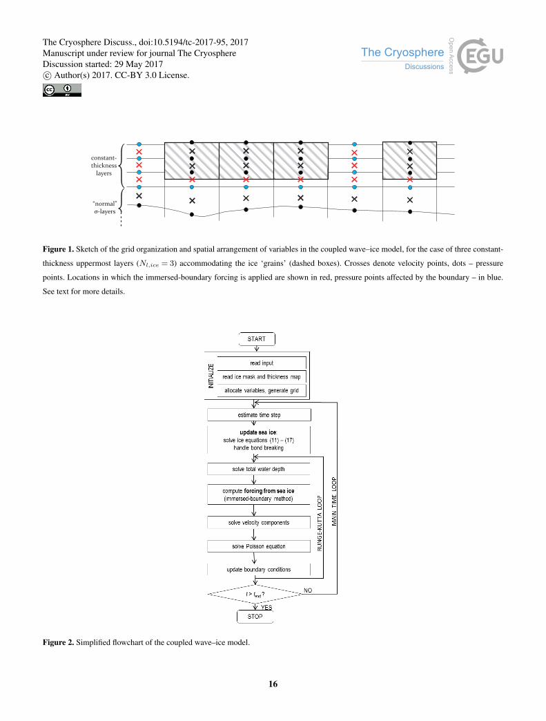
constant-thickness

layers

“normal”-layersσ

Figure 1. Sketch of the grid organization and spatial arrangement of variables in the coupled wave–ice model, for the case of three constant-

thickness uppermost layers (Nl,ice = 3) accommodating the ice ‘grains’ (dashed boxes). Crosses denote velocity points, dots – pressure

points. Locations in which the immersed-boundary forcing is applied are shown in red, pressure points affected by the boundary – in blue.

See text for more details.

Figure 2. Simplified flowchart of the coupled wave–ice model.

16


(a) (b)0

10

20

30

40

50

Tim

e (s

)

-1

-0.5

0

0.5

1

0 100 200 300 400 500

Distance from floe edge (m)

0

0.5

1

Am

pl. o

f zi (

cm)

0

10

20

30

40

50

Tim

e (s

)

0

500

1000

1500

2000

2500

3000

3500

0 100 200 300 400 500


0

2000

4000

Am

pl. o

f σt (

Pa)

σt,max

Figure 3. Simulated space–time variability of the ice vertical displacement zi (a) and the tensile stress σt (b) for an ice floe with length

Lo = 500 m; ice thickness hi = 0.5 m, open-water wavelength Lw,0 = 42 m. Lower diagrams show the amplitude of zi and σt in function

of the distance from the ice edge. Magenta dot in (b) marks σt,max.

(a) (b)

0 0.5 1 1.5 2 2.5 3 3.5

Ice thickness (m)

0

1000

2000

3000

4000

5000

6000

7000

σt,m

ax (

Pa)

Lo = 10 m

Lo = 20 m

Lo = 25 m

Lo = 250 m

0 0.5 1 1.5 2 2.5 3 3.5

Ice thickness (m)

4

6

8

10

12

14

16

18

20

Loca

tion

of σ

t,max

(m

)

Lo = 10 m

Lo = 20 m

Lo = 25 m

Lo = 250 m

(c) (d)

101 102

Floe length (m)

0

1000

2000

3000

4000

5000

6000

7000

σt,m

ax (

Pa)

hi = 0.5 m

hi = 1.0 m

hi = 2.0 m

101 102

Floe length (m)

2

4

6

8

10

12

14

16

18

Loca

tion

of σ

t,max

(m

)

hi = 0.5 m

hi = 1.0 m

hi = 2.0 m

Figure 4. Simulated maximum tensile stress σt,max (a,c) and location (distance from the up-wave ice edge) at which it occurs (b,d) for

different ice thickness hi and floe length Lo values; open-water wavelength Lw,0 = 42 m. Note that the x-axis in (c,d) is logarithmic.

17


(a) (b)

101 102

Floe length (m)

0

500

1000

1500

2000

2500

3000

3500

4000

σt,m

ax (

Pa)

Lw,0 = 84 m

Lw,0 = 63 m

Lw,0 = 42 m

Lw,0 = 25 m

101 102

Floe length (m)

2

3

4

5

6

7

8

9

Loca

tion

of σ

t,max

(m

)

Lw,0 = 84 m

Lw,0 = 63 m

Lw,0 = 42 m

Lw,0 = 25 m

(c) (d)

101 102

Floe length (m)

0

1000

2000

3000

4000

5000

6000

7000

σt,m

ax (

Pa)

Lw,0 = 84 m

Lw,0 = 63 m

Lw,0 = 42 m

Lw,0 = 25 m

101 102

Floe length (m)

2

4

6

8

10

12

14

Loca

tion

of σ

t,max

(m

)

Lw,0 = 84 m

Lw,0 = 63 m

Lw,0 = 42 m

Lw,0 = 25 m

Figure 5. Simulated maximum tensile stress σt,max (a,c) and location (distance from the upwave ice edge) at which it occurs (b,d) for

different floe length Lo and open-water wavelength Lw,0 values; ice thickness hi = 0.5 m (a,b) and hi = 1.0 m (c,d). Note that the x-axis is

logarithmic.

(a) (b)

0 100 200 300 400 500


0

500

1000

1500

2000

2500

3000

3500

4000

Am

plitu

de o

f σt (

Pa)

Lo = 5 m

Lo = 10 m

Lo = 15 m

Lo = 20 m

Lo = 25 m

Lo = 50 m

Lo = 100 m

Lo = 250 m

Lo = 500 m

0 5 10 15 20 25 30


0

500

1000

1500

2000

2500

3000

3500

4000

Am

plitu

de o

f σt (

Pa)

Lo = 5 m

Lo = 10 m

Lo = 15 m

Lo = 20 m

Lo = 25 m

Lo = 50 m

Lo = 100 m

Lo = 250 m

Lo = 500 m

Figure 6. Amplitude of the tensile stress σt in function of the distance from the upwave ice edge for different floe length Lo; open-water

wavelength Lw,0 = 42 m, ice thickness hi = 0.5 m. The plot in (b) is a close-up of the region to the left of the dashed line in (a).

18


(a) (b)

0 100 200 300 400 500


0

50

100

150

Tim

e (s

)

0

500

1000

1500

2000

2500

50 100 150


10

15

20

25

30

35

40

45T

ime

(s)

0

500

1000

1500

2000

2500

Figure 7. Simulated space–time variability of the tensile stress σt for an ice floe with length Lo = 500 m undergoing progressive breaking;

ice thickness hi = 0.5 m, open-water wavelength Lw,0 = 42 m, bond strength 2500 Pa. The plot in (b) is a subset of that in (a); breaking

events are marked with magenta dots, broken bonds with dashed lines.

0 100 200 300 400 500


0

1000

2000

3000

Am

pl. o

f σt (

Pa)

(a)

0 100 200 300 400 500


0

0.2

0.4

0.6

0.8

Am

pl. o

f zi (

cm) (b)

without breakingwith breaking

Figure 8. Amplitude of the tensile stress σt (a) and vertical ice displacement (b) in simulations without and with ice breaking. Floe length

Lo = 500 m, ice thickness hi = 0.5 m, open-water wavelength Lw,0 = 42 m, bond strength 2500 Pa.

19


(a) (b)

0 100 200 300 400 500


0

50

100

150

200

Tim

e (s

)

0

100

200

300

400

500

600

700

800

40 60 80 100 120 140


60

65

70

75

80

85

90

95

Tim

e (s

)

0

100

200

300

400

500

600

700

800

Figure 9. As in Fig. 7, but for irregular incoming waves with Jonswap energy spectrum (wave height and peak period corresponding to those

of sine waves used in simulation from Fig. 7).

(a)

50 100 150


10

15

20

25

30

35

40

45

Tim

e (s

)

0

500

1000

1500

2000

2500

40 60 80 100 120


0

1000

2000

σt (

Pa)

(b)before breaking0.01s after breaking0.02s after breaking

40 60 80 100 120


0

1000

2000

σt (

Pa)

(c)

Figure 10. Comparison of the model behavior in simulations with instantaneous and “delayed” bond breaking: space–time variability of the

tensile stress σt in a simulation analogous to that shown in Fig. 7, but with instantaneous bond breaking (a); and details of σt in vicinity

of a selected breaking event from a simulation with instantaneous (b) and “delayed” (c) bond breaking. The curves in (b,c) show σt along

a selected fragment of the ice floe before (blue) and shortly after (red and yellow) breaking, dashed black lines mark the location where

breaking took place.

20


Table 1. Model parameters used in the simulations in Section 3.

Variable Value

Constant parameters:

Water depth H 10 m

Basin length 1500 m

Horizontal grid size ∆x 0.5 m

Number of σ-layers Nl 30

Number of “ice layers” Nl,ice max{3,3hi}Width of sponge layers 125 m

Internal-wavemaker location 290 m

Bond length parameter λ 0.5

Normal to shear stiffness ratio λns 1.5

Young’s modulus Eb 1.0 · 109 Pa

Time step ratio γt 150

Wave amplitude a 0.025 m

Variable parameters:

Floe length Lo 5–500 m

Ice thickness hi 0.3–3.0 m

Open-water wavelength Lw,0 25–84 m

Bond tensile strength σt,br 1500–3000 Pa

(∞ in simulations without breaking)

21


Documents

Wave-induced stress and breaking of sea ice in a coupled