Wavefront aberration measurements and corrections … aberration... · Wavefront aberration measurements and ... Donald Gavel,4 Daren Dillon,4 Scot Olivier,5 and Joel Kubby1 1Jack

Wavefront aberration measurements and corrections through thick tissue using fluorescent

microsphere reference beacons

Oscar Azucena,1,*

Justin Crest,2 Jian Cao,

2 William Sullivan,

2 Peter Kner,

3

Donald Gavel,4 Daren Dillon,

4 Scot Olivier,

5 and Joel Kubby

1

1Jack Baskin School of Engineering, Univ. of California, Santa Cruz, 1156 High St., Santa Cruz, CA 95064, USA 2Molecular, Cell, and Developmental Biology, Univ. of California, Santa Cruz, 1156 High St., CA 95064, USA

3 Department of Biochemistry and Biophysics, University of California, San Francisco, 600-16th St., Box 2240, CA 94158, USA

4Laboratory for Adaptive Optics, University of California, 1156 High St., Santa Cruz CA 95064, USA 5Physics and Advanced Technologies, Lawrence Livermore National Laboratory,

7000 East Avenue, Livermore, CA 94550, USA *[email protected]

Abstract: We present a new method to directly measure and correct the aberrations introduced when imaging through thick biological tissue. A Shack-Hartmann wavefront sensor is used to directly measure the wavefront error induced by a Drosophila embryo. The wavefront measurements are taken by seeding the embryo with fluorescent microspheres used as “artificial guide-stars.” The wavefront error is corrected in ten millisecond steps by applying the inverse to the wavefront error on a micro-electro-mechanical deformable mirror in the image path of the microscope. The results show that this new approach is capable of improving the Strehl ratio by 2 times on average and as high as 10 times when imaging through 100 µm of tissue. The results also show that the isoplanatic half-width is approximately 19 µm resulting in a corrected field of view 38 µm in diameter around the guide-star.

©2010 Optical Society of America

OCIS codes: (220.1080) Adaptive optics; (160.2540) Fluorescent; (010.7350) Wavefront sensing.

References and links

1. A. Van Helden, “The Invention of the Telescope,” Trans. Am. Phil. Soc. 67, 20–21 (1977). 2. A. Dunn, and R. Richards-Kortum, “Three-dimensional computation of light scattering from cells,” IEEE J. Sel.

Top. Quantum Electron. 2(4), 898–905 (1996). 3. M. Schwertner, M. J. Booth, and T. Wilson, “Specimen-induced distortions in light microscopy,” J. Microsc.

228(1), 97–102 (2007). 4. M. Schwertner, M. J. Booth, M. A. Neil, and T. Wilson, “Measurement of specimen-induced aberrations of

biological samples using phase stepping interferometry,” J. Microsc. 213(1), 11–19 (2004). 5. A. Neil Campbell and Jane B. Reece, Biology, Benjamin Cummings, San Francisco, 2002. 6. H. W. Babcock, “The possibility of compensating astronomical seeing,” Publ. Astron. Soc. Pac. 65, 229–236

(1953). 7. J. W. Hardy, Adaptive Optics for Astronomical Telescopes, Oxford University Press, New York, 1998. 8. J. Liang*, B. Grimm, S. Goelz, and J. F. Bille, “Objective measurement of wave aberrations of the human eye

with the use of a Hartmann-Shack wave-front sensor,” J. Opt. Soc. Am. A 11(7), 1949 (1994). 9. J. Liang, D. R. Williams, and D. T. Miller, “Supernormal vision and high-resolution retinal imaging through

adaptive optics,” J. Opt. Soc. Am. A 14(11), 2884–2892 (1997). 10. M. J. Booth, “Adaptive optics in microscopy,” Philos. Trans. R. Soc. London, Ser. A 365(1861), 2829–2843

(2007). 11. M. Feierabend, M. Rückel, and W. Denk, “Coherence-gated wave-front sensing in strongly scattering samples,”

Opt. Lett. 29(19), 2255–2257 (2004). 12. L. Diaz Santana Haro, and J. C. Dainty, “Single-pass measurements of the wave-front aberrations of the human

eye by use of retinal lipofuscin autofluorescence,” Opt. Lett. 24(1), 61–63 (1999). 13. J. L. Beverage, R. V. Shack, and M. R. Descour, “Measurement of the three-dimensional microscope point

spread function using a Shack-Hartmann wavefront sensor,” J. Microsc. 205(1), 61–75 (2002).

#129768 - $15.00 USD Received 10 Jun 2010; revised 14 Jul 2010; accepted 16 Jul 2010; published 30 Jul 2010(C) 2010 OSA 2 August 2010 / Vol. 18, No. 16 / OPTICS EXPRESS 17521

14. Invitrogen Corporation, Fluorescence SpectraViewer, http://www.invitrogen.com/site/us/en/home/support/Research-Tools/Fluorescence-SpectraViewer.reg.us.html, Last Accessed: 3/24/2010.

15. W. F. Rothwell, and W. Sullivan, Fluorescent analysis of Drosophila embryos. In Drosophila Protocols. W. Sullivan, M. Ashburner, and R.S. Hawley, editors. Cold Spring Harbor Laboratory Press, Cold Spring Harbor, NY, pp. 141–157 (2000).

16. S. Guldbrand, C. Simonsson, M. Goksör, M. Smedh, and M. B. Ericson, “Two-photon fluorescence correlation microscopy combined with measurements of point spread function; investigations made in human skin,” Opt. Express 18(15), 15289–15302 (2010).

17. A. DeMarais, D. Oldis, and J. M. Quattro, “Matrotrophic Transfer of Fluorescent Microspheres in Poeciliid Fishes,” Copeia 2005(3), 632–636 (2005).

18. B. A. Rowning, J. Wells, M. Wu, J. C. Gerhart, R. T. Moon, and C. A. Larabell, “Microtubule-mediated transport of organelles and localization of beta-catenin to the future dorsal side of Xenopus eggs,” Proc. Natl. Acad. Sci. U.S.A. 94(4), 1224–1229 (1997).

19. R. F. Kalpin, D. R. Daily, and W. Sullivan, “Use of dextran beads for live analysis of the nuclear division and nuclear envelope breakdown/reformation cycles in the Drosophila embryo,” Biotechniques 17(4), 730–733 (1994).

20. O. Azucena, J. Cao, J. Crest, W. Sullivan, P. Kner, S. O. Don Gavel, and J. Kubby, “Implementation of adaptive optics in fluorescent microscopy using wavefront sensing and correction,” Proc. SPIE 7595, 75950I (2010).

21. S. Thomas, T. Fusco, A. Tokovinin, M. Nicolle, V. Michau, and G. Rousset, “Comparison of centroid computation algorithms in a Shack-Hartmann sensor,” Mon. Not. R. Astron. Soc. 371(1), 323–336 (2006).

22. A. Lisa Poyneer, D. T. Gavel, J. M. Brase, Fast wave-front reconstruction in large adaptive optics systems with use of the Fourier transform,” J. Opt. Soc. Am. A 19, 2100–2111 (2003).

23. J. Porter, H. Queener, J. Lin, K. Thorn, and A. Awwal, Adaptive Optics for Vision Science, Wiley-Interscience, New Jersey, 2006.

24. L. A. Poyneer, “Scene-based Shack-Hartmann wave-front sensing: analysis and simulation,” Appl. Opt. 42(29), 5807–5815 (2003).

25. Peter Kner, Jian Cao, Oscar Azucena, Justin Crest, Zvi Kam, John Sedat, David Agard, Don Gavel, S. Olivier, Joel Kubby and William Sullivan, “Optical Aberrations in Drosophila Embryos,” submitted to J. Biomed. Opt. (2010).

26. C. R. Vogel, and Q. Yang, “Modeling, simulation, and open-loop control of a continuous facesheet MEMS deformable mirror,” J. Opt. Soc. Am. A 23(5), 1074–1081 (2006).

1. Introduction

Changes in the index of refraction due to tissue composition limit the resolving power of biological microscopy [1–4]. This effect is more pronounced in deep tissue imaging where the light travels through many layers of cellular structures including cytoplasm and the plasma membrane. Many important biological processes occur in deep tissue such as stem cell division, neurogenesis and the key developmental events following fertilization [5]. A method that can be used to improve deep tissue imaging is Adaptive Optics (AO). AO is a technique used in astronomy to directly measure and correct the aberration introduced by turbulence in the optical path [6,7]. AO has also been applied to vision science to enhance our understanding of the human eye [8,9].

The idea for using adaptive optics for microscopy is relatively new and a lot of work is still needed [10]. Most adaptive optics microscope systems so far have not directly measured the wavefront due to the complexity of adding a wavefront sensor in an optical system and the lack of natural point-source references such as the “guide-stars” used in astronomy and vision science. Instead, most AO scanning microscopy systems have corrected the wavefront by optimizing a signal received at a photo-detector by using a hill-climbing algorithm [10]. While other research programs are using adaptive optics in microscopy, there has been no prior work using implanted “guide-star” reference beacons and wavefront sensing to directly measure the physical quantity that is corrected by the deformable mirror, as we have done here. The use of artificial “guide-stars” has been successfully demonstrated and adopted as the standard in most fields in which AO is used, but has only rarely been implemented in biological imaging. Marcus Feierabend et al. developed a method of obtaining direct wavefront measurements in highly scattering samples by using a short pulse of light [11]. The length of the pulse served to distinguish scattered light coming from the focus by using a coherence-gating technique. This method worked well but it requires a sample with a relatively high scattering coefficient. Booth described some of the difficulties associated with the utilization of a Shack-Hartmann Wavefront Sensor (SHWS) in AO microscopy [10]. Most


of these difficulties can be overcome if a suitable fluorescent point source reference beacon could be found. Haro et al. developed a technique that utilized the natural fluorescence of lipofuscin in the eye to form an incoherent point like source for conventional Shack-Hartmann sensing [12]. However the use of lipofuscin is limited to retinal imaging in adult patients where lipusfuscin accumulates in the retina with age. Beverage, Shack, and Descour used a fluorescent microsphere to measure the three dimensional point spread function of a 40X objective by measuring the wavefront at the aperture of the objective [13], but they did not extend these measurements to wavefront measurements for light propagating through biological samples. A method for directly measuring and correcting the wavefront aberrations induced by a Drosophila embryo using a Shack-Hartmann wavefront sensor, a deformable mirror and light emitted from an embedded florescent microsphere will be presented. The Drosophila embryo is well suited to analysis as it is approximately 200 µm in diameter, rich in cytoplasm and amenable to experimental manipulation.

Fluorescent microspheres, with a large variety of colors, are typically used in biology to study different biological characteristics [14–19]. The microspheres can be engineered with coatings to preserve them in different conditions and can be made to target different biological tissues, organelles, cell walls, or other biological structures [14]. They can be introduced into the sample by different mechanisms such as negative pressure injection, pressure injection, matrotrophycally, diffusion and others [16–18]. In particular, fluorescent microspheres have been injected previously in Drosophila embryos [19]. Sufficiently small fluorescent microspheres, as described below, are diffraction limited when imaged by the Shack-Hartmann wavefront sensor enabling their use as point source reference beacons for the operation of the Shack-Hartmann wavefront sensor. Azucena et al. shows that multiple beads can also be used to directly measure the wavefront [20]. The wavefront measurements from multiple beads and a single bead differ only in the higher-order aberrations (e.g. above the 7

th

order Zernike).

2. Methods

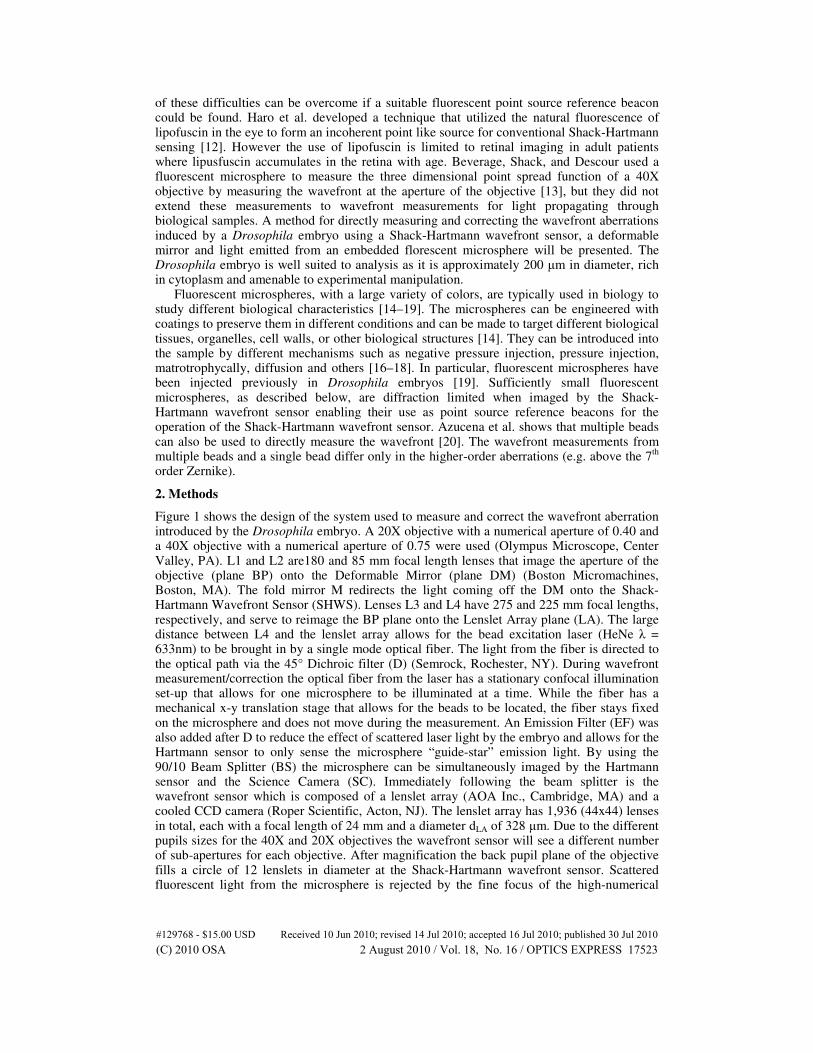
Figure 1 shows the design of the system used to measure and correct the wavefront aberration introduced by the Drosophila embryo. A 20X objective with a numerical aperture of 0.40 and a 40X objective with a numerical aperture of 0.75 were used (Olympus Microscope, Center Valley, PA). L1 and L2 are180 and 85 mm focal length lenses that image the aperture of the objective (plane BP) onto the Deformable Mirror (plane DM) (Boston Micromachines, Boston, MA). The fold mirror M redirects the light coming off the DM onto the Shack-Hartmann Wavefront Sensor (SHWS). Lenses L3 and L4 have 275 and 225 mm focal lengths, respectively, and serve to reimage the BP plane onto the Lenslet Array plane (LA). The large distance between L4 and the lenslet array allows for the bead excitation laser (HeNe λ = 633nm) to be brought in by a single mode optical fiber. The light from the fiber is directed to the optical path via the 45° Dichroic filter (D) (Semrock, Rochester, NY). During wavefront measurement/correction the optical fiber from the laser has a stationary confocal illumination set-up that allows for one microsphere to be illuminated at a time. While the fiber has a mechanical x-y translation stage that allows for the beads to be located, the fiber stays fixed on the microsphere and does not move during the measurement. An Emission Filter (EF) was also added after D to reduce the effect of scattered laser light by the embryo and allows for the Hartmann sensor to only sense the microsphere “guide-star” emission light. By using the 90/10 Beam Splitter (BS) the microsphere can be simultaneously imaged by the Hartmann sensor and the Science Camera (SC). Immediately following the beam splitter is the wavefront sensor which is composed of a lenslet array (AOA Inc., Cambridge, MA) and a cooled CCD camera (Roper Scientific, Acton, NJ). The lenslet array has 1,936 (44x44) lenses in total, each with a focal length of 24 mm and a diameter dLA of 328 µm. Due to the different pupils sizes for the 40X and 20X objectives the wavefront sensor will see a different number of sub-apertures for each objective. After magnification the back pupil plane of the objective fills a circle of 12 lenslets in diameter at the Shack-Hartmann wavefront sensor. Scattered fluorescent light from the microsphere is rejected by the fine focus of the high-numerical


aperture objective and does not impact the centroids of the Shack-Hartmann spots as described below.

Fig. 1. Microscope set up with a Deformable Mirror (DM) and a Shack-Hartmann Wavefront Sensor (SHWS). Dichroic filter (D) allows the laser light to be focused onto the sample. Beam Splitter (BS) allows for both the Science Camera (SC) and the SHWS to simultaneously see the fluorescent microsphere.

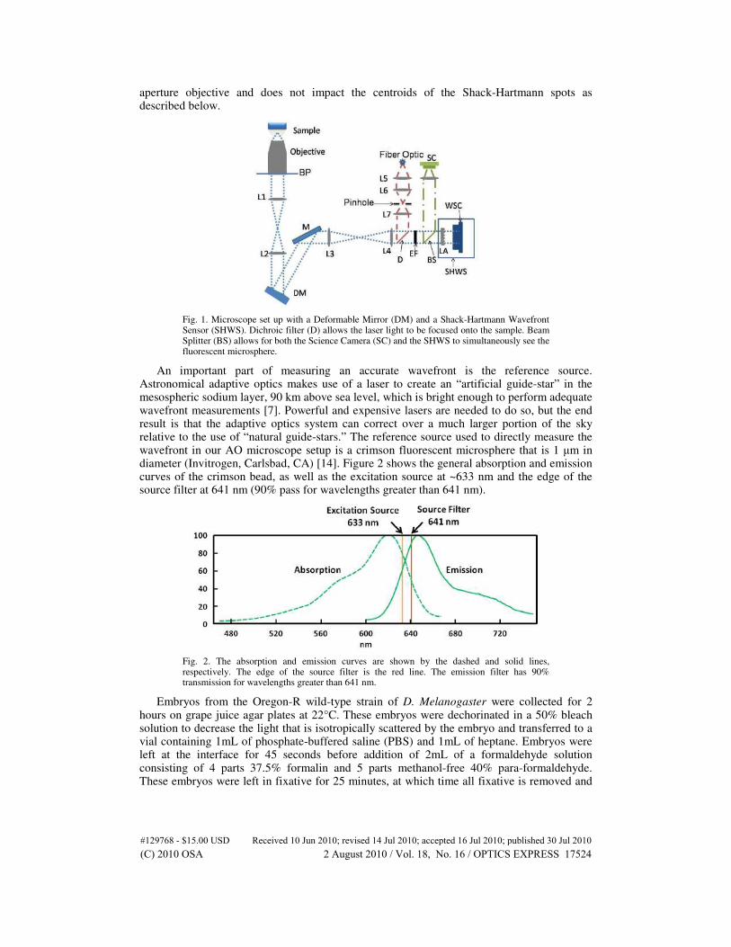
An important part of measuring an accurate wavefront is the reference source. Astronomical adaptive optics makes use of a laser to create an “artificial guide-star” in the mesospheric sodium layer, 90 km above sea level, which is bright enough to perform adequate wavefront measurements [7]. Powerful and expensive lasers are needed to do so, but the end result is that the adaptive optics system can correct over a much larger portion of the sky relative to the use of “natural guide-stars.” The reference source used to directly measure the wavefront in our AO microscope setup is a crimson fluorescent microsphere that is 1 µm in diameter (Invitrogen, Carlsbad, CA) [14]. Figure 2 shows the general absorption and emission curves of the crimson bead, as well as the excitation source at ~633 nm and the edge of the source filter at 641 nm (90% pass for wavelengths greater than 641 nm).

Fig. 2. The absorption and emission curves are shown by the dashed and solid lines, respectively. The edge of the source filter is the red line. The emission filter has 90% transmission for wavelengths greater than 641 nm.

Embryos from the Oregon-R wild-type strain of D. Melanogaster were collected for 2 hours on grape juice agar plates at 22°C. These embryos were dechorinated in a 50% bleach solution to decrease the light that is isotropically scattered by the embryo and transferred to a vial containing 1mL of phosphate-buffered saline (PBS) and 1mL of heptane. Embryos were left at the interface for 45 seconds before addition of 2mL of a formaldehyde solution consisting of 4 parts 37.5% formalin and 5 parts methanol-free 40% para-formaldehyde. These embryos were left in fixative for 25 minutes, at which time all fixative is removed and


the embryos are hand devittelinized and stored in PBTA (1x PBS, 1% Bovine Serum Albumin (BSA), 0.05% Triton X-100, 0.02% Sodium Azide) [15].

Following the typical embryo preparation for imaging as described above, the embryos were desiccated for 6 minutes. This step helps to maintain a negative pressure inside the embryo and allows for the microsphere solution to stay in the embryo upon injection. The microspheres were diluted in a 1:1000 phosphate-buffered saline solution. A microinjection manipulator and pull glass capillary tube were used to inject the solution into the embryo.

3. Results

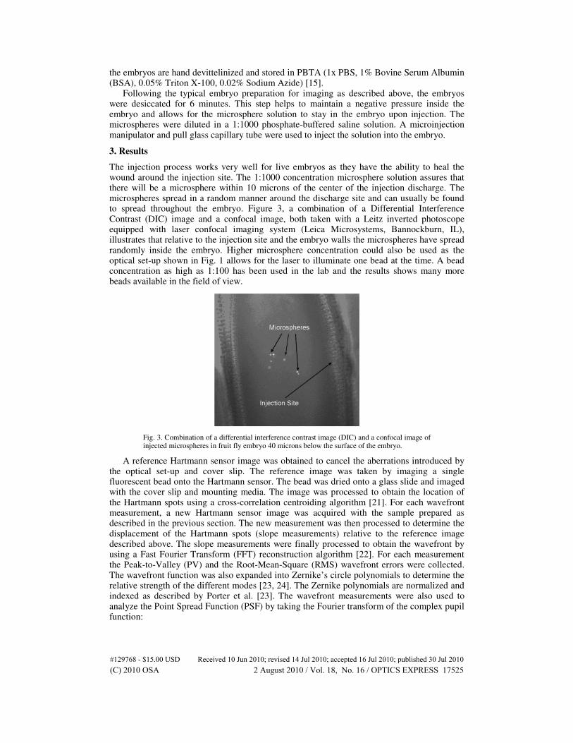
The injection process works very well for live embryos as they have the ability to heal the wound around the injection site. The 1:1000 concentration microsphere solution assures that there will be a microsphere within 10 microns of the center of the injection discharge. The microspheres spread in a random manner around the discharge site and can usually be found to spread throughout the embryo. Figure 3, a combination of a Differential Interference Contrast (DIC) image and a confocal image, both taken with a Leitz inverted photoscope equipped with laser confocal imaging system (Leica Microsystems, Bannockburn, IL), illustrates that relative to the injection site and the embryo walls the microspheres have spread randomly inside the embryo. Higher microsphere concentration could also be used as the optical set-up shown in Fig. 1 allows for the laser to illuminate one bead at the time. A bead concentration as high as 1:100 has been used in the lab and the results shows many more beads available in the field of view.

Fig. 3. Combination of a differential interference contrast image (DIC) and a confocal image of injected microspheres in fruit fly embryo 40 microns below the surface of the embryo.

A reference Hartmann sensor image was obtained to cancel the aberrations introduced by the optical set-up and cover slip. The reference image was taken by imaging a single fluorescent bead onto the Hartmann sensor. The bead was dried onto a glass slide and imaged with the cover slip and mounting media. The image was processed to obtain the location of the Hartmann spots using a cross-correlation centroiding algorithm [21]. For each wavefront measurement, a new Hartmann sensor image was acquired with the sample prepared as described in the previous section. The new measurement was then processed to determine the displacement of the Hartmann spots (slope measurements) relative to the reference image described above. The slope measurements were finally processed to obtain the wavefront by using a Fast Fourier Transform (FFT) reconstruction algorithm [22]. For each measurement the Peak-to-Valley (PV) and the Root-Mean-Square (RMS) wavefront errors were collected. The wavefront function was also expanded into Zernike’s circle polynomials to determine the relative strength of the different modes [23, 24]. The Zernike polynomials are normalized and indexed as described by Porter et al. [23]. The wavefront measurements were also used to analyze the Point Spread Function (PSF) by taking the Fourier transform of the complex pupil function:


{ }

2

,

2

0, 0

2( ', ') exp ( ', ')

( , )( ', ')

x y

f f

FT P x y i w x y

PSF x yFT P x y

ξ ηλ λ

ξ η

πλ

= =

= =

∗

= (1)

Where P is one inside the pupil and zero everywhere else, x’ and y’ are the coordinates at the pupil plane, ξ and η are the spatial frequency in the transform domain, x and y are the coordinates at the image plane, w is the wavefront measurement, and λ is the wavelength at which the measurement was taken.

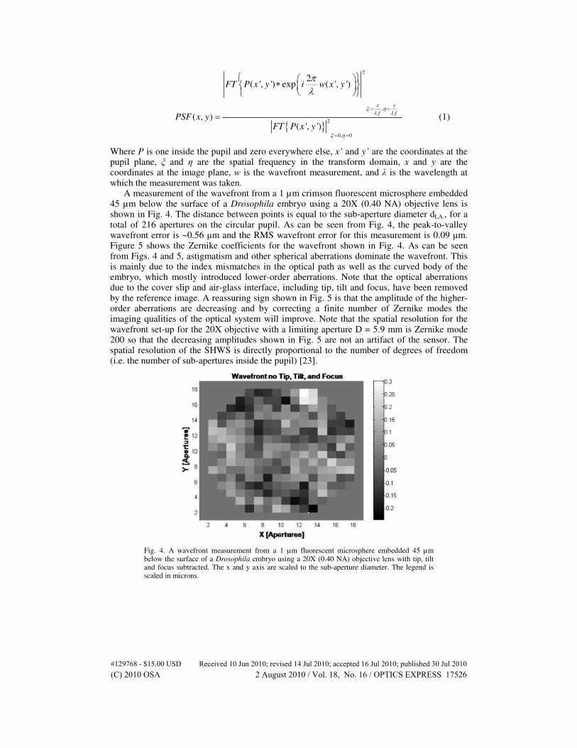
A measurement of the wavefront from a 1 µm crimson fluorescent microsphere embedded 45 µm below the surface of a Drosophila embryo using a 20X (0.40 NA) objective lens is shown in Fig. 4. The distance between points is equal to the sub-aperture diameter dLA., for a total of 216 apertures on the circular pupil. As can be seen from Fig. 4, the peak-to-valley wavefront error is ~0.56 µm and the RMS wavefront error for this measurement is 0.09 µm. Figure 5 shows the Zernike coefficients for the wavefront shown in Fig. 4. As can be seen from Figs. 4 and 5, astigmatism and other spherical aberrations dominate the wavefront. This is mainly due to the index mismatches in the optical path as well as the curved body of the embryo, which mostly introduced lower-order aberrations. Note that the optical aberrations due to the cover slip and air-glass interface, including tip, tilt and focus, have been removed by the reference image. A reassuring sign shown in Fig. 5 is that the amplitude of the higher-order aberrations are decreasing and by correcting a finite number of Zernike modes the imaging qualities of the optical system will improve. Note that the spatial resolution for the wavefront set-up for the 20X objective with a limiting aperture D = 5.9 mm is Zernike mode 200 so that the decreasing amplitudes shown in Fig. 5 are not an artifact of the sensor. The spatial resolution of the SHWS is directly proportional to the number of degrees of freedom (i.e. the number of sub-apertures inside the pupil) [23].

Fig. 4. A wavefront measurement from a 1 µm fluorescent microsphere embedded 45 µm below the surface of a Drosophila embryo using a 20X (0.40 NA) objective lens with tip, tilt and focus subtracted. The x and y axis are scaled to the sub-aperture diameter. The legend is scaled in microns.


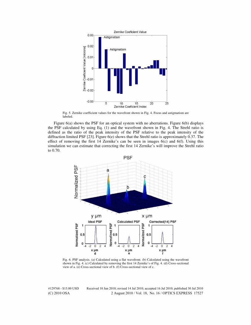
Fig. 5. Zernike coefficient values for the wavefront shown in Fig. 4. Focus and astigmatism are labeled.

Figure 6(a) shows the PSF for an optical system with no aberrations. Figure 6(b) displays the PSF calculated by using Eq. (1) and the wavefront shown in Fig. 4. The Strehl ratio is defined as the ratio of the peak intensity of the PSF relative to the peak intensity of the diffraction limited PSF [23]. Figure 6(e) shows that the Strehl ratio is approximately 0.37. The effect of removing the first 14 Zernike’s can be seen in images 6(c) and 6(f). Using this simulation we can estimate that correcting the first 14 Zernike’s will improve the Strehl ratio to 0.70.

Fig. 6. PSF analysis. (a) Calculated using a flat wavefront. (b) Calculated using the wavefront shown in Fig. 4. (c) Calculated by removing the first 14 Zernike’s of Fig. 4. (d) Cross-sectional view of a. (e) Cross-sectional view of b. (f) Cross-sectional view of c.


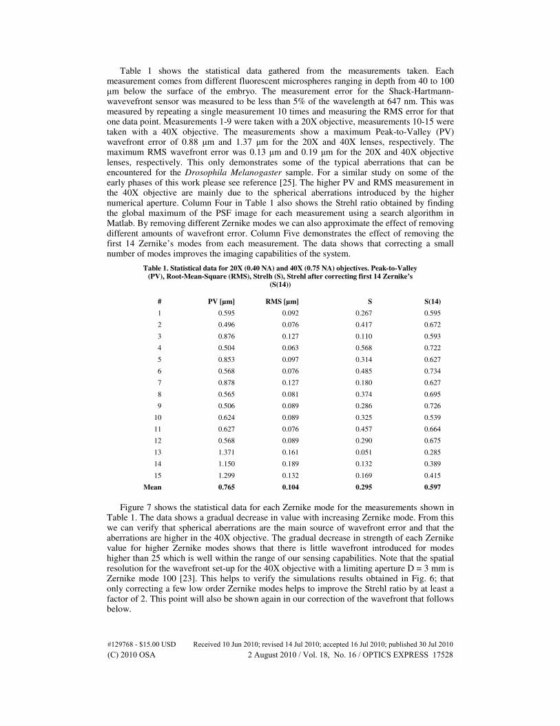
Table 1 shows the statistical data gathered from the measurements taken. Each measurement comes from different fluorescent microspheres ranging in depth from 40 to 100 µm below the surface of the embryo. The measurement error for the Shack-Hartmann-wavevefront sensor was measured to be less than 5% of the wavelength at 647 nm. This was measured by repeating a single measurement 10 times and measuring the RMS error for that one data point. Measurements 1-9 were taken with a 20X objective, measurements 10-15 were taken with a 40X objective. The measurements show a maximum Peak-to-Valley (PV) wavefront error of 0.88 µm and 1.37 µm for the 20X and 40X lenses, respectively. The maximum RMS wavefront error was 0.13 µm and 0.19 µm for the 20X and 40X objective lenses, respectively. This only demonstrates some of the typical aberrations that can be encountered for the Drosophila Melanogaster sample. For a similar study on some of the early phases of this work please see reference [25]. The higher PV and RMS measurement in the 40X objective are mainly due to the spherical aberrations introduced by the higher numerical aperture. Column Four in Table 1 also shows the Strehl ratio obtained by finding the global maximum of the PSF image for each measurement using a search algorithm in Matlab. By removing different Zernike modes we can also approximate the effect of removing different amounts of wavefront error. Column Five demonstrates the effect of removing the first 14 Zernike’s modes from each measurement. The data shows that correcting a small number of modes improves the imaging capabilities of the system.

Table 1. Statistical data for 20X (0.40 NA) and 40X (0.75 NA) objectives. Peak-to-Valley (PV), Root-Mean-Square (RMS), Strelh (S), Strehl after correcting first 14 Zernike’s

(S(14))

# PV [µm] RMS [µm] S S(14)

1 0.595 0.092 0.267 0.595

2 0.496 0.076 0.417 0.672

3 0.876 0.127 0.110 0.593

4 0.504 0.063 0.568 0.722

5 0.853 0.097 0.314 0.627

6 0.568 0.076 0.485 0.734

7 0.878 0.127 0.180 0.627

8 0.565 0.081 0.374 0.695

9 0.506 0.089 0.286 0.726

10 0.624 0.089 0.325 0.539

11 0.627 0.076 0.457 0.664

12 0.568 0.089 0.290 0.675

13 1.371 0.161 0.051 0.285

14 1.150 0.189 0.132 0.389

15 1.299 0.132 0.169 0.415

Mean 0.765 0.104 0.295 0.597

Figure 7 shows the statistical data for each Zernike mode for the measurements shown in Table 1. The data shows a gradual decrease in value with increasing Zernike mode. From this we can verify that spherical aberrations are the main source of wavefront error and that the aberrations are higher in the 40X objective. The gradual decrease in strength of each Zernike value for higher Zernike modes shows that there is little wavefront introduced for modes higher than 25 which is well within the range of our sensing capabilities. Note that the spatial resolution for the wavefront set-up for the 40X objective with a limiting aperture D = 3 mm is Zernike mode 100 [23]. This helps to verify the simulations results obtained in Fig. 6; that only correcting a few low order Zernike modes helps to improve the Strehl ratio by at least a factor of 2. This point will also be shown again in our correction of the wavefront that follows below.


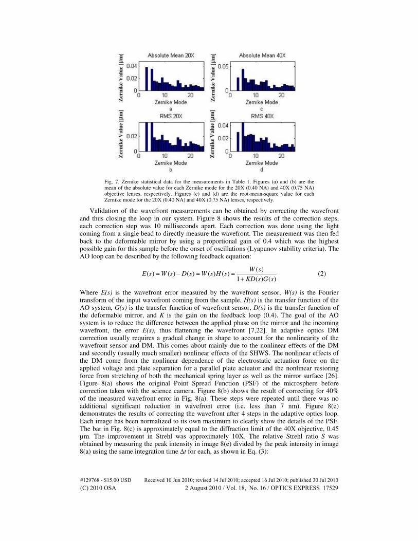
Fig. 7. Zernike statistical data for the measurements in Table 1. Figures (a) and (b) are the mean of the absolute value for each Zernike mode for the 20X (0.40 NA) and 40X (0.75 NA) objective lenses, respectively. Figures (c) and (d) are the root-mean-square value for each Zernike mode for the 20X (0.40 NA) and 40X (0.75 NA) lenses, respectively.

Validation of the wavefront measurements can be obtained by correcting the wavefront and thus closing the loop in our system. Figure 8 shows the results of the correction steps, each correction step was 10 milliseconds apart. Each correction was done using the light coming from a single bead to directly measure the wavefront. The measurement was then fed back to the deformable mirror by using a proportional gain of 0.4 which was the highest possible gain for this sample before the onset of oscillations (Lyapunov stability criteria). The AO loop can be described by the following feedback equation:

( )

( ) ( ) ( ) ( ) ( )1 ( ) ( )

W sE s W s D s W s H s

KD s G s= − = =

+ (2)

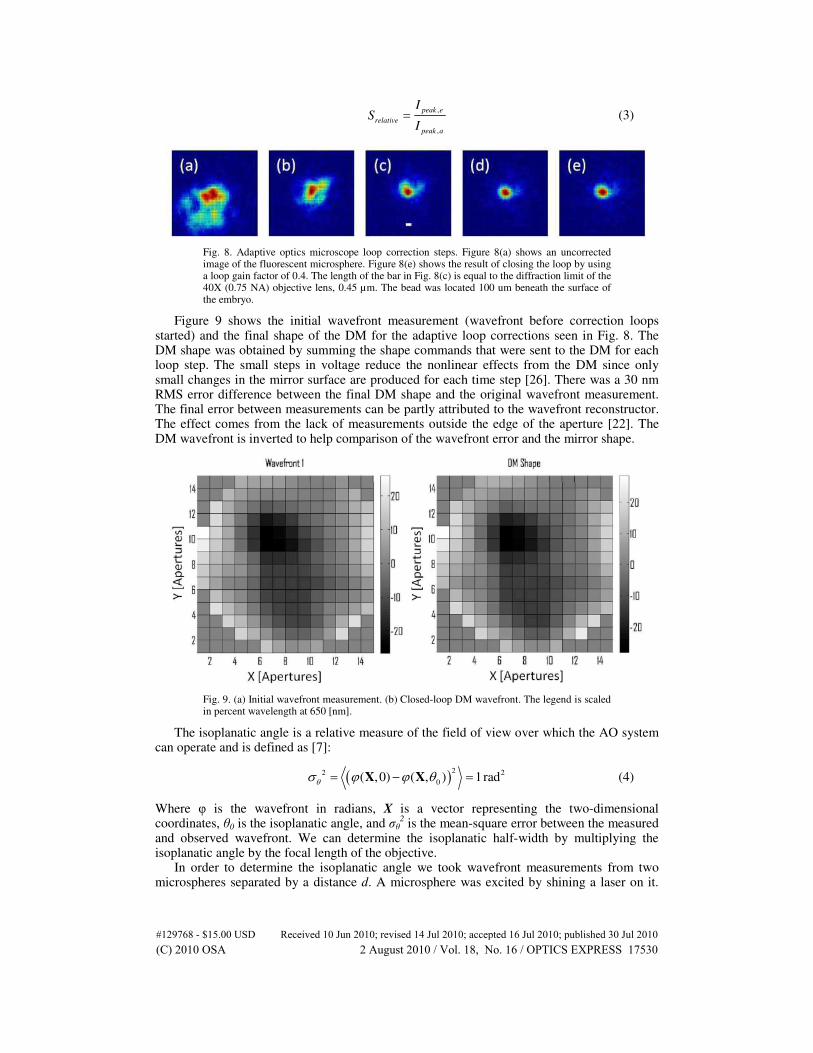
Where E(s) is the wavefront error measured by the wavefront sensor, W(s) is the Fourier transform of the input wavefront coming from the sample, H(s) is the transfer function of the AO system, G(s) is the transfer function of wavefront sensor, D(s) is the transfer function of the deformable mirror, and K is the gain on the feedback loop (0.4). The goal of the AO system is to reduce the difference between the applied phase on the mirror and the incoming wavefront, the error E(s), thus flattening the wavefront [7,22]. In adaptive optics DM correction usually requires a gradual change in shape to account for the nonlinearity of the wavefront sensor and DM. This comes about mainly due to the nonlinear effects of the DM and secondly (usually much smaller) nonlinear effects of the SHWS. The nonlinear effects of the DM come from the nonlinear dependence of the electrostatic actuation force on the applied voltage and plate separation for a parallel plate actuator and the nonlinear restoring force from stretching of both the mechanical spring layer as well as the mirror surface [26]. Figure 8(a) shows the original Point Spread Function (PSF) of the microsphere before correction taken with the science camera. Figure 8(b) shows the result of correcting for 40% of the measured wavefront error in Fig. 8(a). These steps were repeated until there was no additional significant reduction in wavefront error (i.e. less than 7 nm). Figure 8(e) demonstrates the results of correcting the wavefront after 4 steps in the adaptive optics loop. Each image has been normalized to its own maximum to clearly show the details of the PSF. The bar in Fig. 8(c) is approximately equal to the diffraction limit of the 40X objective, 0.45 µm. The improvement in Strehl was approximately 10X. The relative Strehl ratio S was obtained by measuring the peak intensity in image 8(e) divided by the peak intensity in image 8(a) using the same integration time ∆t for each, as shown in Eq. (3):


,

,

peak e

relative

peak a

IS

I= (3)

Fig. 8. Adaptive optics microscope loop correction steps. Figure 8(a) shows an uncorrected image of the fluorescent microsphere. Figure 8(e) shows the result of closing the loop by using a loop gain factor of 0.4. The length of the bar in Fig. 8(c) is equal to the diffraction limit of the 40X (0.75 NA) objective lens, 0.45 µm. The bead was located 100 um beneath the surface of the embryo.

Figure 9 shows the initial wavefront measurement (wavefront before correction loops started) and the final shape of the DM for the adaptive loop corrections seen in Fig. 8. The DM shape was obtained by summing the shape commands that were sent to the DM for each loop step. The small steps in voltage reduce the nonlinear effects from the DM since only small changes in the mirror surface are produced for each time step [26]. There was a 30 nm RMS error difference between the final DM shape and the original wavefront measurement. The final error between measurements can be partly attributed to the wavefront reconstructor. The effect comes from the lack of measurements outside the edge of the aperture [22]. The DM wavefront is inverted to help comparison of the wavefront error and the mirror shape.

Fig. 9. (a) Initial wavefront measurement. (b) Closed-loop DM wavefront. The legend is scaled in percent wavelength at 650 [nm].

The isoplanatic angle is a relative measure of the field of view over which the AO system can operate and is defined as [7]:

( )22 2

0( ,0) ( , ) 1radθσ ϕ ϕ θ= − =X X (4)

Where φ is the wavefront in radians, X is a vector representing the two-dimensional coordinates, θ0 is the isoplanatic angle, and σθ

2 is the mean-square error between the measured

and observed wavefront. We can determine the isoplanatic half-width by multiplying the isoplanatic angle by the focal length of the objective.

In order to determine the isoplanatic angle we took wavefront measurements from two microspheres separated by a distance d. A microsphere was excited by shining a laser on it.


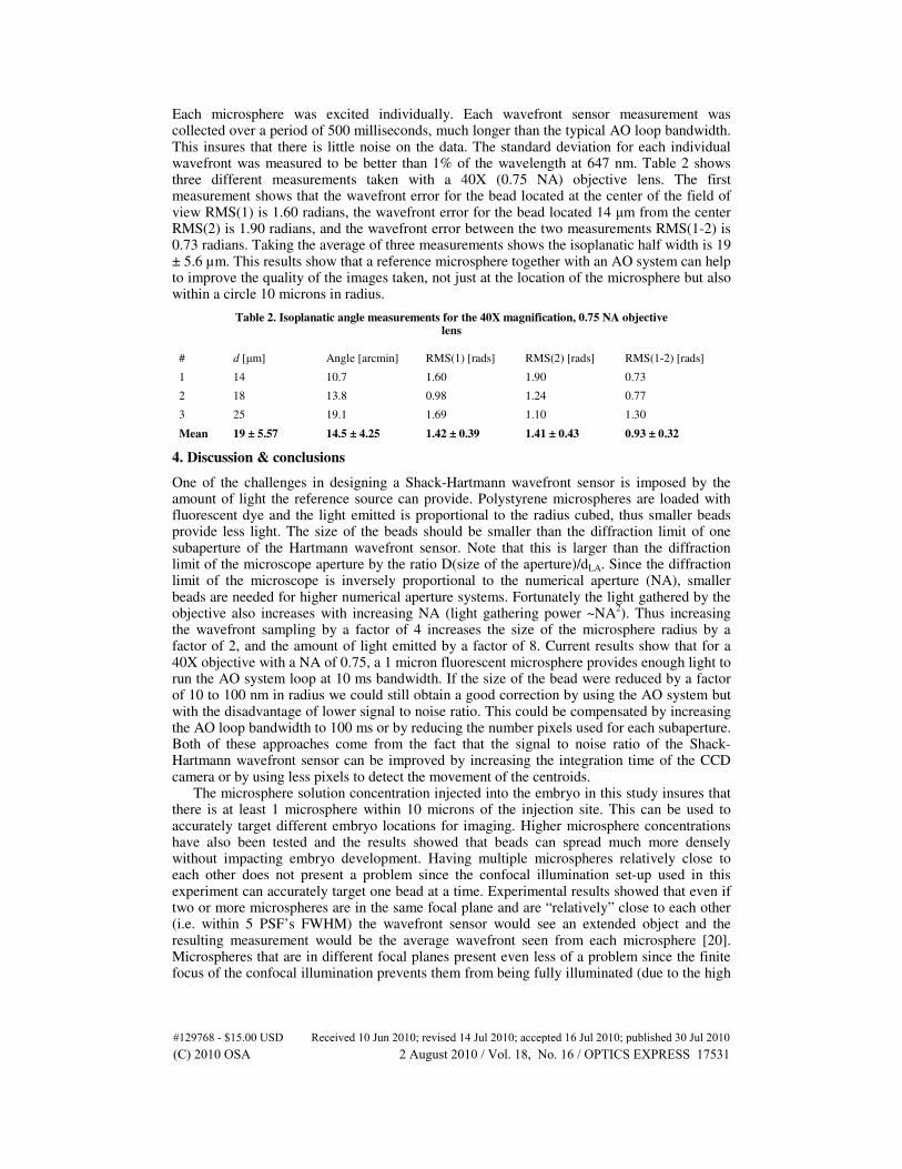
Each microsphere was excited individually. Each wavefront sensor measurement was collected over a period of 500 milliseconds, much longer than the typical AO loop bandwidth. This insures that there is little noise on the data. The standard deviation for each individual wavefront was measured to be better than 1% of the wavelength at 647 nm. Table 2 shows three different measurements taken with a 40X (0.75 NA) objective lens. The first measurement shows that the wavefront error for the bead located at the center of the field of view RMS(1) is 1.60 radians, the wavefront error for the bead located 14 µm from the center RMS(2) is 1.90 radians, and the wavefront error between the two measurements RMS(1-2) is 0.73 radians. Taking the average of three measurements shows the isoplanatic half width is 19 ± 5.6 µm. This results show that a reference microsphere together with an AO system can help to improve the quality of the images taken, not just at the location of the microsphere but also within a circle 10 microns in radius.

Table 2. Isoplanatic angle measurements for the 40X magnification, 0.75 NA objective lens

# d [µm] Angle [arcmin] RMS(1) [rads] RMS(2) [rads] RMS(1-2) [rads]

1 14 10.7 1.60 1.90 0.73

2 18 13.8 0.98 1.24 0.77

3 25 19.1 1.69 1.10 1.30

Mean 19 ± 5.57 14.5 ± 4.25 1.42 ± 0.39 1.41 ± 0.43 0.93 ± 0.32

4. Discussion & conclusions

One of the challenges in designing a Shack-Hartmann wavefront sensor is imposed by the amount of light the reference source can provide. Polystyrene microspheres are loaded with fluorescent dye and the light emitted is proportional to the radius cubed, thus smaller beads provide less light. The size of the beads should be smaller than the diffraction limit of one subaperture of the Hartmann wavefront sensor. Note that this is larger than the diffraction limit of the microscope aperture by the ratio D(size of the aperture)/dLA. Since the diffraction limit of the microscope is inversely proportional to the numerical aperture (NA), smaller beads are needed for higher numerical aperture systems. Fortunately the light gathered by the objective also increases with increasing NA (light gathering power ~NA

2). Thus increasing

the wavefront sampling by a factor of 4 increases the size of the microsphere radius by a factor of 2, and the amount of light emitted by a factor of 8. Current results show that for a 40X objective with a NA of 0.75, a 1 micron fluorescent microsphere provides enough light to run the AO system loop at 10 ms bandwidth. If the size of the bead were reduced by a factor of 10 to 100 nm in radius we could still obtain a good correction by using the AO system but with the disadvantage of lower signal to noise ratio. This could be compensated by increasing the AO loop bandwidth to 100 ms or by reducing the number pixels used for each subaperture. Both of these approaches come from the fact that the signal to noise ratio of the Shack-Hartmann wavefront sensor can be improved by increasing the integration time of the CCD camera or by using less pixels to detect the movement of the centroids.

The microsphere solution concentration injected into the embryo in this study insures that there is at least 1 microsphere within 10 microns of the injection site. This can be used to accurately target different embryo locations for imaging. Higher microsphere concentrations have also been tested and the results showed that beads can spread much more densely without impacting embryo development. Having multiple microspheres relatively close to each other does not present a problem since the confocal illumination set-up used in this experiment can accurately target one bead at a time. Experimental results showed that even if two or more microspheres are in the same focal plane and are “relatively” close to each other (i.e. within 5 PSF’s FWHM) the wavefront sensor would see an extended object and the resulting measurement would be the average wavefront seen from each microsphere [20]. Microspheres that are in different focal planes present even less of a problem since the finite focus of the confocal illumination prevents them from being fully illuminated (due to the high


NA) and hence they are not the brightest object in the field of view. Microspheres that are in different focal planes do show up as a background light in the wavefront sensor camera. It has been shown by Thomas et al. [21] that a robust centroiding algorithm, like the cross-correlation technique used here, does not sense the background and only detects the brightest object in the field of view, be it an extended or point source. This still holds true even for a very small signal to noise ratio (i.e. the background would add to the peak of the Hartmann spot centroid but it does not move it). The same can be said for light that is being scattered inside the embryo. It adds to the background but it does not change the wavefront sensor measurement.

An emerging field in adaptive optics is tomography AO, where multiple light sources together with multiple SHWS are used. The information from each wavefront sensor is then processed using a reconstructor to acquire a tomographic image of the changes in the index of refraction in the optical path [7]. One of the advantages of using tomography AO is that it can provide information on the depth dependence of variations in the index of refraction in the tissue thus allowing for the AO system to correct for the wavefront aberrations only in the optical path. This technique can also extend the isoplanatic angle by correcting wavefront aberrations that are common to a larger field of view. By depositing multiple fluorescent beads into the biological sample and using multiple wavefront sensors we can also apply the tomographic techniques that have been developed for astronomical AO.

An adaptive optics microscope was designed using a Shack-Hartmann wavefront sensor and a Micro-Electro-Mechanical Systems (MEMS) deformable mirror to directly measure and correct the wavefront error induced by a Drosophila embryo. The wavefront measurements were taken by using a new method of seeding an embryo with fluorescent microspheres that are used as “artificial guide-stars.” The maximum wavefront error for a 40X magnification, 0.75 NA objective lens was 1.37 µm and 0.19 µm for the peak-to-valley and root-mean-square, respectively. The residual wavefront error after correction was 7 nm RMS. The measurements also show that the isoplanatic half-width is approximately 19 µm resulting in a field of view of 38 µm in total. Analysis of the data demonstrated that this approach can improve the Strehl ratio by 2 times on average and as high as 10 times when imaging through 100 µm of tissue.

Acknowledgments

This research has been supported by the National Science Foundation Science & Technology Center for Adaptive Optics (CfAO), managed by the University of California at Santa Cruz under Cooperative Agreement No. AST 9876783 and by funding from the National Science Foundation Center for Biophotonics Science & Technology (CBST), managed by the University of California, Davis, under Cooperative Agreement No. PHY 0120999. This research was also supported by a grant from the California Institute for Regenerative Medicine (Grant Number RT1-01095-1). The contents of this publication are solely the responsibility of the authors and do not necessarily represent the official views of CIRM or any other agency of the State of California. Oscar Azucena was supported by a University of California Systemwide Biotechnology Research & Education Program GREAT Training Grant #2008-19, Jian Cao and Justin Crest were supported by NIH (GM046409), William Sullivan by the California Institute for Quantitative Biosciences (QB3) and Peter Kner by the Center for Biophotonics Science and Technology.


Documents

Wavefront aberration measurements and corrections … aberration... · Wavefront aberration measurements and ... Donald Gavel,4 Daren Dillon,4 Scot Olivier,5 and Joel Kubby1 1Jack