Embed Size (px)
Citation preview
Wavelet Analysis and Its Applications The subject of wavelet analysis has recently drawn a great deal of attention from mathematical scientists in various disciplines. It is creating a common link between mathematicians, physicists, and electrical engineers. This book series will consist of both monographs and edited volumes on the theory and applications of this rapidly developing subject. Its objective is to meet the needs of academic, industrial, and governmental researchers, as well as to provide instructional material for teaching at both the undergrad-uate and graduate levels.
This fourth volume of the series is a compilation of twelve papers de-voted to wavelet analysis of geophysical processes. In addition to an intro-ductory review article written by the editors, this volume covers such important areas as atmospheric turbulence, seismic data analysis, detec-tion of signals in noisy environments, multifractal analysis, and analysis of long memory geophysical processes. The series editor is grateful to Profes-sor Foufoula-Georgiou and Dr. Kumar for their effort in compiling and ed-iting this excellent volume, and would like to thank the authors for their very fine contributions.
This is a volume in WAVELET ANALYSIS A N D ITS APPLICATIONS
CHARLES K. CHUI, SERIES EDITOR Texas A&M University, College Station, Texas
A list of titles in this series appears at the end of this volume.
Wavelets in Geophysics
Edited by
Efi Foufoula-Georgiou Si. Anthony Falls Hydraulic Laboratory Department of Civil Engineering University of Minnesota Minneapolis, Minnesota
Praveen Kumar Universities Space Research Association Hydrological Sciences Branch NASA-Goddard Space Flight Center Greenbelt, Maryland
® ACADEMIC PRESS
San Diego New York Boston London Sydney Tokyo Toronto
This book is printed on acid-free paper, fe)
Copyright © 1994 by ACADEMIC PRESS, INC. All Rights Reserved. No part of this publication may be reproduced or transmitted in any form or by any means, electronic or mechanical, including photocopy, recording, or any information storage and retrieval system, without permission in writing from the publisher.
Academic Press, Inc. A Division of Harcourt Brace & Company 525 B Street, Suite 1900, San Diego, California 92101-4495
United Kingdom Edition published by Academic Press Limited 24-28 Oval Road, London NW1 7DX
Library of Congress Cataloging-in-Publication Data
Wavelets in geophysics / edited by Efi Foufoula-Georgiou, Praveen Kumar.
p. cm. — (Wavelet analysis and its applications ; v. 4) Includes bibliographical references and index. ISBN 0-12-262850-0 I. Foufoula-Georgiou, Efi, II. Kumar, Praveen. III. Series.
QC806.W38 1994 550'.l'5152433-dc20 94-16953
CIP
PRINTED IN THE UNITED STATES OF AMERICA 94 95 96 97 98 99 MM 9 8 7 6 5 4 3 2 1
To Katerina, Thomas
and Ilina
Contributors
Numbers in parentheses indicate the pages on which the authors'contributions begin.
J O H N D. ALBERTSON (81), Hydrologie Science, University of California at Davis, Davis, California 95616
KEVIN E. BREWER (213), Department of Geological Sciences/172, University of Nevada, Reno, Reno, Nevada 89557
YVES BRUNET (129), Laboratoire de Bioclimatologie, INRA, BP 81, 33883 Villenave dOrnon, France
CHIA R. CHU (81), Department of Civil Engineering, National Central University, Chungli, Taiwan
SERGE COLLINEAU (129), Laboratoire de Bioclimatologie, INRA, BP 81, 33883 Villenave dOrnon, France
ANTHONY DAVIS (249), Universities Space Research Association, NASA-Goddard Space Flight Center, Greenbelt, Maryland 20771
E F I FOUFOULA-GEORGIOU (1), St. Anthony Falls Hydraulic Laboratory, Department of Civil Engineering, University of Minnesota, Minneapolis, Minnesota 55414
NlMAL K. K. GAMAGE (45), Program in Atmospheric and Oceanic Sciences, Astrophysics, Planetary and Atmospheric Sciences Department, University of Colorado, Boulder, Colorado 80309
PETER GUTTORP (325), Department of Statistics, University of Washington, Seattle, Washington 98195
CARL R. HAGELBERG (45), National Center for Atmospheric Research, Boulder, Colorado 80307
J. F. HOWELL (107), Oceanic and Atmospheric Sciences, Oregon State University, Corvallis, Oregon 97331
GABRIEL G. KATUL (81), School of the Environment, Duke University, Durham, North Carolina 27708
PRAVEEN KUMAR (1), Universities Space Research Association, Hydrological Sciences Branch, NASA-Goddard Space Flight Center, Greenbelt, Maryland 20771
SARAH A. LITTLE (167), Department of Geology and Geophysics, Woods Hole Océanographie Institution, Woods Hole, Massachusetts 02543
ix
x Contributors
PAUL C. LIU (151), NOAA Great Lakes Environmental Research Laboratory, Ann Arbor, Michigan 48109
L. MAHRT (107), Oceanic and Atmospheric Sciences, Oregon State University, Corvallis, Oregon 97331
ALEXANDER MARSHAK (249), Science Systems and Applications, Inc., Lanham, Maryland 20706
MARC B. PARLANGE (81), Hydrologie Science, and Department of Agricultural
and Biological Engineering, University of California at Davis, Davis, California 95616
DONALD B. PERCIVAL (325), Applied Physics Laboratory, University of Washington, Seattle, Washington 98195
CHRIS J. PIKE (183), Centre for Cold Ocean Resources Engineering (C-CORE), Memorial University of Newfoundland, St. John's, Newfoundland, Canada AIB 3X5
NAOKI SAITO (299), Schlumberger-Doll Research, Old Quarry Road, Ridgefield, Connecticut 06877, and Department of Mathematics, Yale University, New Haven, Connecticut 06520
STEPHEN W. WHEATCRAFT (213), Department of Geological Sciences/172,
University of Nevada, Reno, Reno, Nevada 89557
WARREN WISCOMBE (249), NASA-Goddard Space Flight Center, Climate and Radiation Branch, Greenbelt, Maryland 20771
Preface
Over the past decade, wavelet transforms have been formalized into a rigorous mathematical framework and have found numerous applications in diverse areas such as harmonic analysis, numerical analysis, signal and image pro-cessing, nonlinear dynamics, fractal and multifractal analysis, and others. Although wavelet transforms originated in geophysics (for the analysis of seismic signals), it is only very recently that they are being used again in the geophysical sciences. Properties that make wavelets attractive are t i m e -frequency localization, orthogonality, multirate filtering, and scale-space analysis, to name a few.
This volume is the first collection of papers using wavelet transforms for the understanding, analysis, and description of geophysical processes. It in-cludes applications of wavelets to atmospheric turbulence, ocean wind waves, characterization of hydraulic conductivity, seafloor bathymetry, seismic data, detection of signals from noisy data, multifractal analysis, and analysis of long memory geophysical processes. Most of the papers included in this volume were presented at the American Geophysical Union (AGU) Spring Meeting in Balti-more, May 1993, in a special Union session organized by us entitled "Applica-tions of Wavelet Transforms in Geophysics." We feel that this volume will serve geophysicists as an introduction to the versatile and powerful wavelet analysis tools and will stimulate further applications of wavelets in geophysics as well as mathematical developments dictated by unique demands of applications.
The first chapter in this volume is a review article by Kumar and Foufoula-Georgiou. The purpose of this article is to provide the unfamiliar reader with a basic introduction to wavelets and key references for further study. Wavelet transforms are contrasted with the Fourier transforms and windowed Fourier transforms that are well known to geophysicists; this contrast highlights the important property of time—frequency localization in wavelet transforms, which is essential for the analysis of nonstationary and transient signals. Continuous and discrete, as well as orthogonal, nonorthogonal, and biortho-gonal wavelet transforms are then reviewed, and the concept of multiresolution analysis is presented. Several examples of one- and two-dimensional wavelets and information on wavelet construction are given. Finally, some sources of available wavelet analysis software packages are included which may help the interested reader get started in exploring wavelets.
The next four chapters present results from the application of wavelet analysis to atmospheric turbulence. In Chapter 2, Hagelberg and Gamage develop a wavelet-based signal decomposition technique that preserves inter-mittent coherent structures. Coherent structures in velocity and temperature in the atmospheric boundary layer account for a large portion of flux transport of momentum, heat, trace chemicals, and particulates. The authors' technique partitions signals into two components: one containing coherent structures characterized by sharp transitions and intermittent occurrence, and the other
xi
X l l Preface
containing the remaining portion of the signal (essentially characterized by smaller length scales and the absence of coherent events). They apply this decomposition to vertical velocity, virtual potential temperature, and buoyancy flux density fields. Chapter 3, by Katul, Albertson, Chu, and Parlange, applies orthonormal wavelets to atmospheric surface layer velocity measurements to describe space-time relations in the inertial subrange. The local nature of the orthonormal wavelet transform in physical space aids the identification of events contributing to inertial subrange intermittency buildup, which can then be suppressed to eliminate intermittency effects on the statistical structure of the inertial subrange.
In Chapter 4, Howell and Mahrt develop an adaptive method for decom-posing a time series into orthogonal modes of variation. In contrast to conven-tional partitioning, the cutoff scales are allowed to vary with record position according to the local physics of the flow by utilizing the Haar wavelet decom-position. For turbulence data, this decomposition is used to distinguish four modes of variation. The two larger modes, determined by spatially constant cutoff scales, are characterized as the mesoscale and large eddy modes. The two smaller scale modes are separated by a scale that depends on the local transport characteristics of the flow. This adaptive cutoff scale separates the transporting eddy mode, responsible for most of the flux, from the nontrans-porting nearly isotropic motions. Chapter 5, by Brunet and Collineau, applies wavelets to the analysis of turbulent motions above a maize crop. Their results indicate that organized turbulence exhibits the same structure above a forest and a maize crop, apart from a scale factor, and supports the interesting pos-tulate that transfer processes over plant canopies are dominated by popula-tions of canopy-scale eddies, with universal characteristics. The authors also propose a methodology for separating turbulence data into large- and small-scale components using the filtering properties of the wavelet transform.
In Chapter 6, Liu applies wavelet spectrum analysis to ocean wind waves. The results reveal significant new insights on wave grouping parameteriza-tions, phase relations during wind wave growth, and detection of wave breaking characteristics. Chapter 7, by Little, demonstrates the usefulness of wavelet analysis in studying seafloor bathymetry and especially identifying the loca-tion and scarp-facing direction of ridge-parallel faulting. In Chapter 8, Pike proposes a wavelet-based methodology for the analysis of high resolution acoustic signals for sub-seabed feature extraction and classification of scatter-ers. The key idea is that of displaying the energy dissipation in the t i m e -frequency plane, which allows a more distinct description of the signal (com-pared to the Fourier transform spectra) and thus provides a better means of extracting seabed properties by correlating them to the attenuation of high resolution acoustic signals. In Chapter 9, Brewer and Wheatcraft investigate the wavelet transform as a tool for reconstructing small-scale variability in hydraulic conductivity fields by incorporating the scale and location informa-tion of each sample when interpolating to a finer grid. The developed multiscale reconstruction method is compared to traditional interpolation schemes and is used to examine the issue of optimum sample size and density for stationary and fractal random fields.
Preface Xlll
Chapter 10, by Davis, Marshak, and Wiscombe, explores the use of wave-lets for multifractal analysis of geophysical phenomena. They show the appli-cability of wavelet transforms to compute simple yet dynamically meaningful statistical properties of one dimensional geophysical series. Turbulent velocity and cloud liquid water content are used as examples to demonstrate the need for stochastic models having both additive (nonstationary) and multiplicative (intermittent) features. Merging wavelet and multifractal analysis seems promising for both wavelet and multifractal communities and is especially promising for geophysics, where many signals show structures at all observa-ble scales and are often successfully described within a multifractal frame-work.
The wavelet transform partitions the frequency axis in a particular way: it iteratively partitions the low-frequency components, leaving the high-fre-quency components intact at each iteration. For some processes or applications this partition might not achieve the best decomposition, as partition of the high-frequency bands might also be necessary. Wavelet packets provide such a partition and are used in Chapter 11, by Saito, for simultaneous signal compression and noise reduction of geophysical signals. A maximum entropy criterion is used to obtain the best basis out of the many bases that the redun-dant wavelet packet representation provides. The method is applied to syn-thetic signals and to some geophysical data, for example, a radioactivity profile of subsurface formation and a migrated seismic section. Finally, in Chapter 12, Percival and Guttorp examine a particular measure of variability for long memory processes (the Allan variance) within the wavelet framework and show that this variance can be interpreted as a Haar wavelet coefficient variance. This suggests an approach to assessing the variability of general wavelet classes which will be useful in the study of power-law processes extensively used for the description of geophysical time series. A fairly extensive bibliog-raphy of wavelet analysis in geophysics is included at the end of this volume.
Several individuals provided invaluable help in the completion of this vol-ume. Special thanks go to the reviewers of the book chapters who volunteered their time and expertise and provided timely and thoughtful reviews. The first author thanks Mike Jasinski, Hydrologie Sciences Branch at NASA-Goddard Space Flight Center and the Universities Space Research Association for their support during the completion of this project. We are grateful to Charu Gupta Kumar, who converted most of the chapters to I^T^X format and typeset and edited the entire volume. Without her expertise and dedication the timely completion of this volume would not have been possible. Finally, we also thank the Academic Press Editor, Peter Renz, for his efficient help during the final stages of this project.
Efi Foufoula-Georgiou Praveen Kumar Minneapolis, Minnesota Greenbelt, Maryland March, 1994
Wavele t Analys i s in Geophys ics : A n Introduct ion
Praveen Kumar and Efi Foufoula-Georgiou
Abstract. Wavelet analysis is a rapidly developing area of mathematical and application-oriented research in many disciplines of science and engineering. The wavelet transform is a localized transform in both space (time) and frequency, and this property can be advantageously used to extract information from a signal that is not possible to unravel with a Fourier or even windowed Fourier transform. Wavelet transforms originated in geophysics in early 1980's for the analysis of seismic signal. After a decade of significant mathematical formalism they are now also being exploited for the analysis of several other geophysical processes such as atmospheric turbulence, space-time rainfall, ocean wind waves, seafloor bathymetry, geologic layered structures, climate change, among others. Due to their unique properties, well suited for the analysis of natural phenomena, it is anticipated that there will be an explosion of wavelet applications in geophysics in the next several years. This chapter provides a basic introduction to wavelet transforms and their most important properties. The theory and applications of wavelets is developing very rapidly and we see this chapter only as a limited basic introduction to wavelets which we hope to be of help to the unfamiliar reader and provide motivation and references for further study.
§1. Pro logue
The concept of wavelet transforms was formalized in early 1980's in a series of papers by Morlet et al. [42, 43], Grossmann and Morlet [24], and Goupillaud, Grossmann and Morlet [23]. Since this formalism and some significant work by Meyer ([38, 39] and references therein), Mallat [30, 31], Daubechies [13, 15], and Chui [6] among others, the wavelets have become pervasive in several diverse areas such as mathematics, physics, digital sig-nal processing, vision, numerical analysis, and geophysics, to name a few. Wavelet transforms are integral transforms using integration kernels called wavelets. These wavelets are essentially used in two ways when studying
Wavelets in Geophysics 1 Efi Foufoula-Georgiou and Praveen Kumar (eds.), pp. 1-43. Copyright 1994 by Academic Press, Inc. All rights of reproduction in any form reserved. ISBN 0-12-262850-0
2 P. Kumar and E. Foufoula-Georgiou
processes or signals: (i) as an integration kernel for analysis to extract information about the process, and (ii) as a basis for representation or characterization of the process. Evidently, in any analysis or representa-tion, the choice of the basis function (or kernel) determines the kind of information tha t can be extracted about the process. This leads us to the following questions: (1) what kind of information can we extract using wavelets? and (2) how can we obtain a representation or description of the process using wavelets?
The answer to the first question lies on the important property of wavelets called time-frequency localization. The advantage of analyzing a signal with wavelets as the analyzing kernels is tha t it enables one to study features of the signal locally with a detail matched to their scale, i.e., broad features on a large scale and fine features on small scales. This property is especially useful for signals tha t are either non-stationary, or have short lived transient components, or have features at different scales, or have singularities. The answer to the second question is based on seeing wavelets as the elementary building blocks in a decomposition or series expansion akin to the familiar Fourier series. Thus, a representation of the process using wavelets is provided by an infinite series expansion of dilated and translated versions of a mother wavelet, each multiplied by an appropriate coefficient. For processes with finite energy this wavelet series expansion is optimal, i.e., it offers an optimal approximation to the original signal, in the least squares sense.
In what follows we give a brief introduction to the mathematics of wavelet transforms and where possible an intuitive explanation of these results. The intention of this introduction is two fold: (i) to provide the unfamiliar reader with a basic introduction to wavelets, and (ii) to prepare the reader to grasp and appreciate the results of the articles tha t follow as well as the potential of wavelet analysis for geophysical processes. At times we have sacrificed mathematical rigor for clarity of presentation in an a t t empt to not obscure the basic idea with too much detail. We also hasten to add tha t this review is far from complete both in terms of the breadth of topics chosen for exposition and in terms of the treatment of these topics. For example, the important topic of wavelet packets has not been discussed (see for example [53], [8], and the article by Saito [50] in this volume). It is recommended tha t the interested reader who is not a mathematician and is meeting wavelet analysis for the first time begins with the book by Meyer [39] and continues with the books by Daubechies [15] and Benedetto and Frazier [3]. There are also several nice introductory articles on several aspects of wavelets, as for example, those by Mallat [30, 31], Rioul and Vetterli [47], and the article by Farge [19] on turbulence, among others. Also, considerable insight can be gained by the nice book reviews by Meyer [40] and Daubechies [18].
Wavelet Analysis in Geophysics: An Introduction 3
This article is organized as follows. Section 2 discusses Fourier and windowed Fourier transforms and introduces continuous wavelet trans-forms and their time-frequency localization properties. In section 3, the wavelet transform is presented as a time-scale transform, and the wavelet variance and covariance (alternatively called wavelet spectrum and cospec-t rum) are discussed. A link is also made between non-stationary processes and wavelet transforms akin to the link between stationary processes and Fourier transforms. Section 4 presents some examples of commonly used one-dimensional wavelets (Haar wavelet, Mexican hat wavelet, and Mor-let wavelet). In section 5, discrete wavelet transforms (orthogonal, non-orthogonal, and biorthogonal) are introduced and the concept of multires-olution analysis presented. In section 6, we present extensions of contin-uous and discrete wavelets in a two-dimensional space. Finally, in section 7 we present some concluding remarks and give information on obtaining available software packages for wavelet analysis.
§2. T i m e - F r e q u e n c y A n a l y s i s
The original motive for the development of wavelet transform was (see [23]) " . . . of devising a method of acquisition, transformation and recording of a seismic trace (i.e., a function of one variable, the time) so as to satisfy the requirements listed below:
1. The contributions of different frequency bands (i.e., of the differ-ent intervals of the Fourier conjugate variable) are kept reasonably separated.
2. This separation is achieved without excessive loss of resolution in the t ime variable (subject, of course, to the limitation of the uncertainty principle).
3. The reconstruction of the original function from its "representation" or "transform" is obtained by a method which is (a) capable of giving arbitrary high precision; (b) is robust, in the sense of being stable under small perturbations. "
The first two conditions essentially characterize the property known as time-frequency localization. Recall tha t although the Fourier transform of a function / (£) , given as
/
oo
f(t)e-^dt, (1) -oo
gives the information about the frequency content of a process or signal, it gives no information about the location of these frequencies in the t ime domain. For example figures la ,b show two signals - the first consisting of
4 P. Kumar and E. Foufoula-Georgiou
50 100 angular frequency
50 100 angular frequency
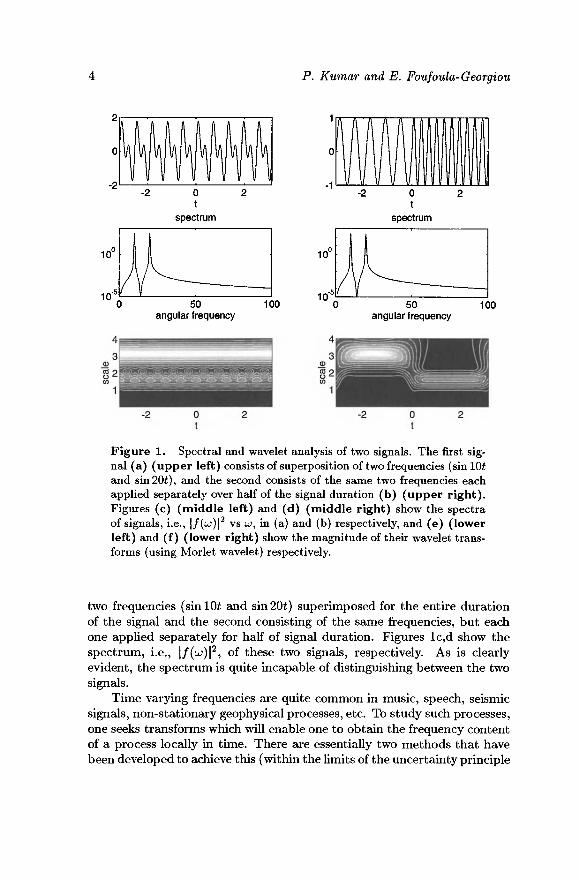
Figure 1. Spectral and wavelet analysis of two signals. The first sig-nal (a) (upper left) consists of superposition of two frequencies (sinlOt and sin20£), and the second consists of the same two frequencies each applied separately over half of the signal duration (b) (upper right). Figures (c) (middle left) and (d) (middle right) show the spectra of signals, i.e., | / (ω) |2 vs � , in (a) and (b) respectively, and (e) (lower left) and (f) (lower right) show the magnitude of their wavelet trans-forms (using Morlet wavelet) respectively.
two frequencies (sin 10t and sin 20t) superimposed for the entire duration of the signal and the second consisting of the same frequencies, but each one applied separately for half of signal duration. Figures lc,d show the spectrum, i.e., | / (o ; ) | 2 , of these two signals, respectively. As is clearly evident, the spectrum is quite incapable of distinguishing between the two signals.
Time varying frequencies are quite common in music, speech, seismic signals, non-stationary geophysical processes, etc. To study such processes, one seeks transforms which will enable one to obtain the frequency content of a process locally in time. There are essentially two methods tha t have been developed to achieve this (within the limits of the uncertainty principle
Wavelet Analysis in Geophysics: An Introduction 5
which states tha t one cannot obtain arbitrary good localization in bo th t ime and frequency): (a) windowed Fourier transform, and (b) wavelet transform. These two methods are discussed in the following subsections. Figures le,f display the magnitude of the wavelet transform of the signals shown in Figures la ,b , and clearly show the ability of the wavelet transform to distinguish between the two signals.
2 .1 . W i n d o w e d Fourier transform
2 .1 .1 . Def ini t ion
In the Fourier transform framework, time localization can be achieved by windowing the da ta at various times, say, using a windowing function #(£), and then taking the Fourier transform. Tha t is, the windowed Fourier transform (also called the short-time fourier transform), G/ (CJ , i ) , is given by
(2)
(3)
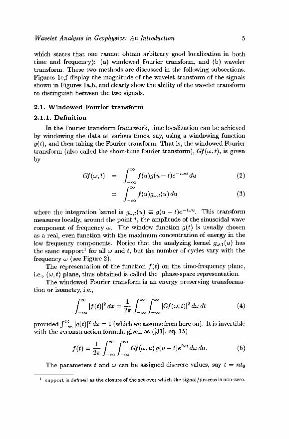
where the integration kernel is gtj,t(u) = g(u — t)e~iuju. This transform measures locally, around the point £, the amplitude of the sinusoidal wave component of frequency � . The window function g(t) is usually chosen as a real, even function with the maximum concentration of energy in the low frequency components. Notice tha t the analyzing kernel <7ω,*(ΐί) has the same support1 for all � and £, but the number of cycles vary with the frequency � (see Figure 2).
The representation of the function f(t) on the time-frequency plane, i.e., (CJ,£) plane, thus obtained is called the phase-space representation.
The windowed Fourier transform is an energy preserving transforma-tion or isometry, i.e.,
(4)
provided / ^ |g(£)|2 dx = 1 (which we assume from here on). It is invertible with the reconstruction formula given as ([31], eq. 15)
(5)
The parameters t and � can be assigned discrete values, say t = nt0
1 support is defined as the closure of the set over which the signal/process is non-zero.
6 P. Kumar and E. Foufoula-Georgiou
Figure 2. Real (solid lines) and imaginary parts (dot-dashed lines) of the analyzing kernel g{t)e~tuJt of the windowed Fourier transform at different frequencies: (a) (top) � = 3, (b) (middle) � = 6 and (c) (bottom) � = 9. The dotted line indicates a Gaussian window function g(t).
and � = mcjo, and we obtain the discrete windowed Fourier transform
/
oo f{u)g{u-nt0)e-im"°udu. (6)
-OO
For the discrete windowed Fourier transform to be invert ible, the condition CJO^O < 2π must hold (see [15], sections 3.4 and 4.1).
2 � . 2 . T ime- frequency local ization
In order to study the time-frequency localization property of the win-dowed Fourier transform, we need to study the properties of |<7ω,*|2 and \çju>,t |2 since they determine the features of f(t) tha t are extracted. Indeed, using Parseval's theorem, equation (3) can be written as
1 f°° A (7)
Wavelet Analysis in Geophysics: An Introduction 7
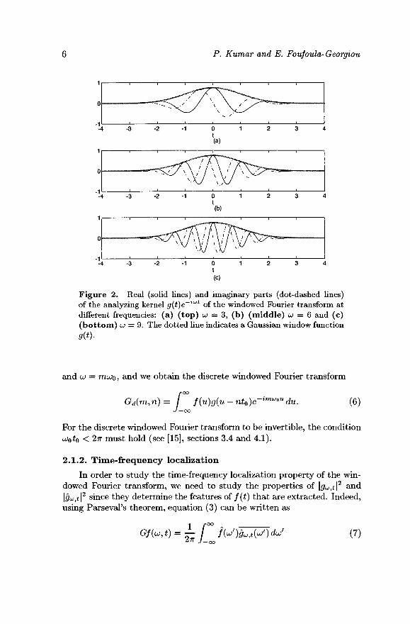
Figure 3. Uncertainties in time (top) and frequency (bottom) lo-calization in a windowed Fourier Transform for a generic function g{t).
where ^ ^ ( u / ) is the Fourier transform of gu,t(u) and overbar indicates complex conjugate. Let us define the s tandard deviations of gu^ and gu^ as ag and ag respectively, i.e.,
and
(9)
These parameters measure the spread of the function | ^ ? < | and \gUjt |, about t and CJ, respectively (see Figure 3). Owing to the uncertainty principle, the products of σ2, and σ | satisfy (see [31])
(10)
(8)
i.e., arbi trary high precision in both t ime and frequency cannot be achieved. The equality in the above equation is achieved only when g(t) is the Gaus-sian, i.e.,
(H) When the Gaussian function is used as a window, the windowed Fourier transform is called the Gabor transform [22].
8 P. Kumar and E. Foufoula-Georgiou
1 ^� 1 8,
� � '
°g .1 � � | 1
1 g) 1
1 ^� 1 8
� 8 .
1 ^� | §
1 ^
1 ^ � | §
� � J
� * U
� 8
to
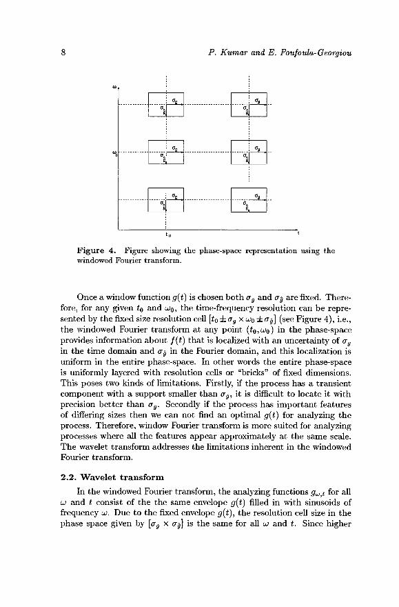
Figure 4. Figure showing the phase-space representation using the windowed Fourier transform.
Once a window function g(t) is chosen both ag and � § are fixed. There-fore, for any given to and CJQ, the time-frequency resolution can be repre-sented by the fixed size resolution cell [t0 ±� 9 � � � ±� 9] (see Figure 4), i.e., the windowed Fourier transform at any point (£o5^o) in the phase-space provides information about f(t) tha t is localized with an uncertainty of ag
in the t ime domain and � 9 in the Fourier domain, and this localization is uniform in the entire phase-space. In other words the entire phase-space is uniformly layered with resolution cells or "bricks" of fixed dimensions. This poses two kinds of limitations. Firstly, if the process has a transient component with a support smaller than σ^, it is difficult to locate it with precision bet ter than ag. Secondly if the process has important features of differing sizes then we can not find an optimal g{i) for analyzing the process. Therefore, window Fourier transform is more suited for analyzing processes where all the features appear approximately at the same scale. The wavelet transform addresses the limitations inherent in the windowed Fourier transform.
2.2 . Wave le t transform
In the windowed Fourier transform, the analyzing functions g„t for all � and t consist of the the same envelope g(t) filled in with sinusoids of frequency � . Due to the fixed envelope g(t), the resolution cell size in the phase space given by [� 9 χ � $] is the same for all � and t. Since higher
Wavelet Analysis in Geophysics: An Introduction 9
frequency (or short wavelength) features have smaller support , it would be desirable to have an analyzing function, say � (�), such tha t its s tandard deviation � � is small when � {�) characterizes high frequency components and vice-versa. This was achieved by decomposing the function f(t) using a two parameter family of functions called wavelets (see [42] and [43]). One of the two parameters is the translation parameter as in the windowed Fourier transform case, but the other parameter is a dilation parameter λ instead of the frequency parameter � .
2 .2 .1 . Def ini t ion
The wavelet transform of a function f(t) with finite energy is defined as the integral transform with a family of functions xjj\)t{u) = ~7� � (� � ^) and is given as
2. zero mean, i.e., J ^ t / ^ ^ d i = 0, although higher order moments
(12)
Here λ is a scale parameter, t a location parameter and the functions ip\jt(u) are called wavelets. In case � \^(� ) is complex, we use the complex con-jugate � � t(u) in the above integration. Changing the value of λ has the effect of dilating (λ > 1) or contracting (λ < 1) the function � (�) (see Fig-ure 5a), and changing t has the effect of analyzing the function f(t) around the point t. The normalizing constant -4^ is chosen so tha t
for all scales λ (notice the identity � (�) = V>i,o(0)· We also choose the normalization j \� (�)\2 dt = 1. The wavelet transform Wf(X^t) is often denoted as the inner product ( / , � \$)-
Notice tha t in contrast to the windowed Fourier transform case, the number of cycles in the wavelet � \^(� ) does not change with the dilation (scale) parameter λ but the support length does. We will see shortly tha t when λ is small, which corresponds to small support length, the wavelet transform picks up higher frequency components and vice-versa.
The choice of the wavelet � {�) is neither unique nor arbitrary. The function � {�) is a function with unit energy chosen so tha t it has:
1. compact support , or sufficiently fast decay, to obtain localization in space;
10 P. Kumar and E. Foufoula-Georgiou
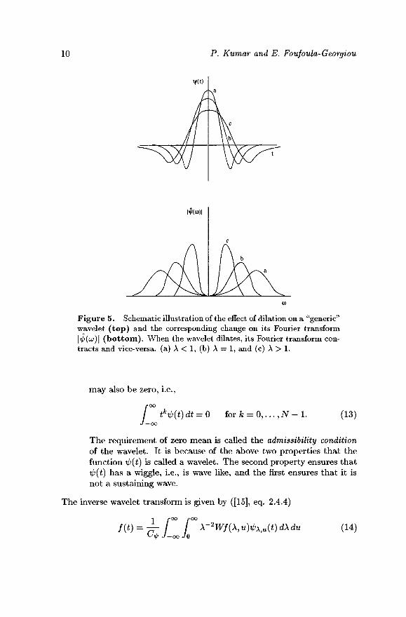
|� (� )|
Figure 5. Schematic illustration of the effect of dilation on a "generic" wavelet (top) and the corresponding change on its Fourier transform |^(ω) | (bottom). When the wavelet dilates, its Fourier transform con-tracts and vice-versa, (a) λ < 1, (b) λ = 1, and (c) λ > 1.
may also be zero, i.e.,
tktp(t) dt = 0 for k = 0 , . . . , N - 1. /
(13)
The requirement of zero mean is called the admissibility condition of the wavelet. It is because of the above two properties tha t the function i/j(t) is called a wavelet. The second property ensures tha t ip(t) has a wiggle, i.e., is wave like, and the first ensures tha t it is not a sustaining wave.
The inverse wavelet transform is given by ([15], eq. 2.4.4)
1 /«oo /*oo
f(t) = 7T / X-2Wf(X,u)<pXiU(t)dXdu W J-ooJO
(14)
Wavelet Analysis in Geophysics: An Introduction 11
where
(15)
The wavelet transform is also an energy preserving transformation, i.e., an isometry (up to a proportionality constant) , tha t is,
(16)
2 .2 .2 . T ime- frequency local ization
In order to understand the behavior of the wavelet transform in the fre-quency domain as well, it is useful to recognize that the wavelet transform W/(A,£), using Parseval's theorem, can be equivalently writ ten as
(17)
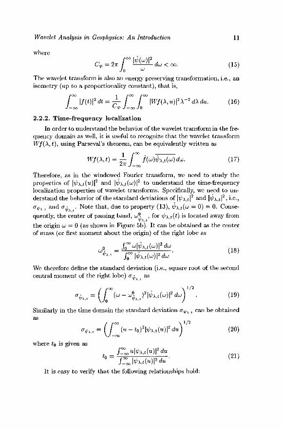
Therefore, as in the windowed Fourier transform, we need to study the properties of \ip\}t(u)\2 and |^A,<(<^)|2 to understand the time-frequency localization properties of wavelet transforms. Specifically, we need to un-derstand the behavior of the s tandard deviations of |^λ,*|2 and |^λ,*|2, i-e-> <� � � >� and σ? . Note that , due to property (13), � \^(� = 0) = 0. Conse-quently, the center of passing band, CJ°~ , for tp\yt(t) is located away from
the origin � = 0 (as shown in Figure 5b). It can be obtained as the center of mass (or first moment about the origin) of the right lobe as
(18)
We therefore define the s tandard deviation (i.e., square root of the second central moment of the right lobe) � τ as
(19)
Similarly in the t ime domain the standard deviation � � � t can be obtained as
(20)
(21)
where to is given as
It is easy to verify tha t the following relationships hold:
12 P. Kumar and E. Foufoula-Georgiou
1. The s tandard deviation � � � t satisfies
� � � ,� = � � � �,� - (22)
2. The s tandard deviation � ;, satisfies
3. The center of passing band αΛ corresponding to the wavelet iß\yt (u)
satisfies the relationship
� °; = - ^ . (24)
From the above relationships one can easily see that as λ increases, i.e., as the function dilates, both � °7 and � ,?, decrease indicating that the center of passing band shifts towards low frequency components and the uncer-tainty also decreases, and vice-versa (see also figure 5). In the phase-space, the resolution cell for the wavelet transform around the point (ίο,ω^ )
is given by [to ± λσ^10 x Alf0 ± A
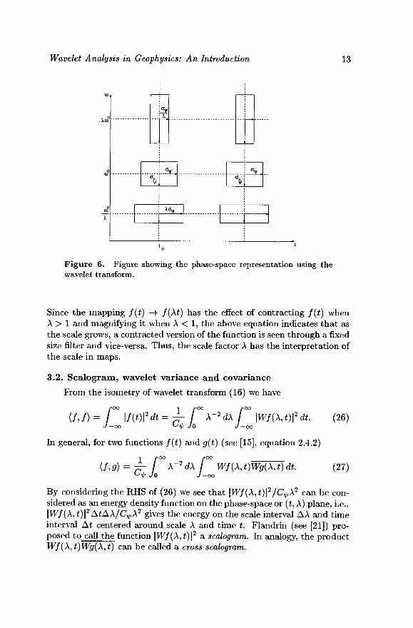
lf0] (see Figure 6) which has variable dimensions depending on the scale parameter λ. However, the area of the resolution cell [� � � t x � ? ] remains independent of the scale or location parameter. In other words, the phase space is layered with resolution cells of varying dimensions which are functions of scale such that they have a constant area. Therefore, due to the uncertainty principle, an increased resolution in the time domain for the time localization of high frequency components comes with a cost: an increased uncertainty in the frequency localization as measured by � ? . One may also interpret the wavelet transform as a mathematical microscope where the magnification is given by 1/λ.
§3. Wavelets and Time-Scale Analysis
3.1. Time-scale transform
Useful information can also be extracted by interpreting the wavelet transform (12) as a time-scale transform. This was well illustrated by Rioul and Vetterli (see [47]) and is sketched below. In the wavelet transform (12) when the scale λ increases, the wavelet becomes more spread out and takes only long time behavior into account, as seen above. However by change of variables, equation (12) can also be written as
(25)
Wavelet Analysis in Geophysics: An Introduction 13
HL
� � ^
Figure 6. Figure showing the phase-space representation using the wavelet transform.
Since the mapping f(t) —> f(Xt) has the effect of contracting f(t) when λ > 1 and magnifying it when λ < 1, the above equation indicates tha t as the scale grows, a contracted version of the function is seen through a fixed size filter and vice-versa. Thus, the scale factor λ has the interpretation of the scale in maps.
3.2 . Sca logram, wavelet variance and covariance
From the isometry of wavelet transform (16) we have
In general, for two functions f(t) and g(t) (see [15], equation 2.4.2)
(26)
(27)
By considering the RHS of (26) we see tha t |W/(A,£) | 2 /C^A2 can be con-sidered as an energy density function on the phase-space or (£, λ) plane, i.e., |W/(A, �)\2� �� � /� � \2 gives the energy on the scale interval Δλ and t ime interval At centered around scale λ and t ime t. Flandrin (see [21]) pro-posed to call the function |W/(A,£)|2 a scalogram. In analogy, the product Wf(\,t)Wg(\,t) can be called a cross scalogram.
14 P. Kumar and E. Foufoula-Georgiou
Equation (26) can also be written as
(28)
(29)
where
gives the energy content of a function f(t) at scale λ, i.e., it gives the marginal density function of energy at different scales λ. The function E(X) has been referred to as wavelet variance (see [4]) or wavelet spectrum (see [25]). In analogy, the function
(30)
has been referred to as wavelet covariance (see [4]) or wavelet cross-spectrum (see [25]).
Notice tha t for a given wavelet ip(t) the center of passing band � °«
at scale λ is related to that at unit scale through the relation (see equation (24))
(31)
Using this relationship, the scale information can be translated to frequency information. Using � � — —� ^ X~2dX and substituting in equation (28) we get
n
(32)
By defining
the above equation can be written as
(33)
(34)
One would therefore expect tha t � '(� ), and thus JE7(A), is related to the power spectrum S/(u>) of f(t). This indeed is the case. It can be shown (see [25]) tha t
(35)
where � � � (� ) is the spectrum of the wavelet at scale λ. Tha t is, E(s) is the weighted average of the power spectrum of f(t) where the weights are
Wavelet Analysis in Geophysics: An Introduction 15
given by the power spectrum of ip\(t). This relation is interesting although in characterizing a process through E(X) or � '{� ), all location information is lost, it does provide certain useful insight ([36], and [27]).
3 .3 . Non- s ta t ionar i t y and t h e Wigner-Vi l l e s p e c t r u m
One reason for the remarkable success of the Fourier transform in the study of stationary stochastic processes is the relationship between the autocorrelation function and the spectrum as illustrated by the following diagram:
T X(t) £± � (� )
R(r) = 8[X(t)X{t - r)] <=i S(u>) = \� (� ) |2
where R(r) and 5(CJ) are the auto-covariance function and the power spec-t rum of the stochastic process X(t), respectively. If an analogous rela-tionship could be developed for non-stationary processes using the wavelet transform, then the properties of the wavelet transform could be harnessed in a more useful way. It turns out that , indeed, such a relationship can be developed.
The wavelet spectrum E(X) or � '(� ) discussed in the previous sec-tion although interesting in its own right, takes us away from the non-stationarity of the process since it is obtained by integrating over t. We, therefore, need something else. This is provided by the Wigner-Ville spec-t rum. Let us define a general (non-stationary) covariance function R(t, s) as
R(t,s)=S[X(t)X(s)].
Then the Wigner-Ville spectrum (WVS) is defined as (see [11] for a dis-cussion of WVS and other time-frequency distributions)
/
oo
� R(t+^,t--)e-iurdT. (36)
The WVSx(t, � ) is an energy density function as
/
oo
WVSx(t,w)duj (37) -co
i.e., we get the instantaneous energy by integrating over all frequencies, and the total energy can be obtained as
(38)
16 P. Kumar and E. Foufoula-Georgiern
The relationship of interest to us is given by the relation between the scalo-gram and the WVS
(39)
i.e., the scalogram can be obtained by affine smoothing (i.e., smoothing at different scales in t and � directions) of the WVS of X with the WVS of the wavelet. This relationship has been developed by Flandrin (see [21]). As of this writing, we are unaware of any inverse relation to obtain the WVSx from the scalogram. We can put the key result of this subsection in the following diagrammatic form:
We, therefore, see tha t there is an inherent link between the study of non-stationary processes and wavelet transforms akin to the link between sta-tionary processes and Fourier transforms.
§4. E x a m p l e s of One-Dimens ional Wave le t s
Due to the flexibility in choosing a wavelet, several functions have been used as wavelets and it would be difficult to provide an exhaustive list. We present here some commonly used wavelets (Haar wavelet, Mexican ha t wavelet, and Morlet wavelet) in one-dimensional applications.
4 .1 . Haar wavelet
The Haar wavelet is the simplest of all wavelets and is given as
(40)
In a one-dimensional discretely sampled signal this wavelet can be seen as performing a differencing operation, i.e., as giving differences of non-overlapping averages of observations. In two dimensions an interpretation of the discrete orthogonal Haar wavelet transform has been given in [28].
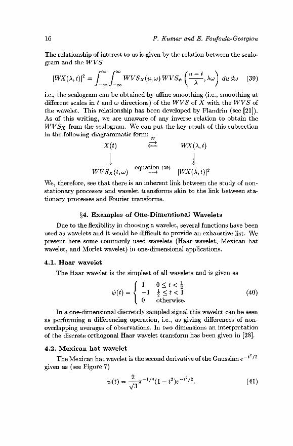
4.2 . M e x i c a n hat wavelet
The Mexican hat wavelet is the second derivative of the Gaussian e~l ' 2
given as (see Figure 7)
(41)
Wavelet Analysis in Geophysics: An Introduction 17
Figure 7. Mexican hat wavelet.
The constant is chosen such tha t || � \\2= 1. This wavelet, being the second derivative of a commonly used smoothing function (the Gaussian), has found application in edge detection (see [34] and [35]).
4 .3 . Mor le t wavelet
The Morlet wavelet is given by
� (� = � � "1 / 4^-^-6"
which is usually approximated as
� * )e
-t2/2
� (� _ _ - 1 / 4 � - � � � * � - * 2 / 2 CJO > 5.
(42)
(43)
Since for � � > 5, the second term in (42) is negligible, i.e., � (�) « 0, satisfying the admissibility condition. By Morlet wavelet we now refer to (43). This wavelet is complex, enabling one to extract information about the ampli tude and phase of the process being analyzed. The constant is chosen so tha t || � \\2= 1. The Fourier transform of (43) is given by
� (� ) = � _ _ - l / 4 -(� -� 0)2/2 (44)
This wavelet has been used quite often in analysis of geophysical pro-cesses (for e.g. see [45]) so we shall study it in a little more detail. The Fourier transform of the scaled wavelet � \}� (�) is given as
λ̂,ο(ω) = � � -�/*� -^-^)'/2 = λ π _ ι / 4 6 - ^ - ω ) * _
This wavelet has the property tha t its Fourier transform is supported
18 P. Kumar and E. Foufoula-Georgiou
Real and imaginary parts of Morlet wavelet
0.5l·
Oh
0.8
0.6
0.2
\y : . .\y
3 (a)
Spectrum of Morlet wavelet
-2 0 2 frequency
10 (b)
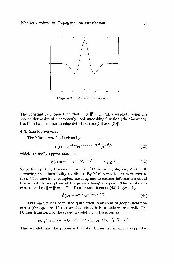
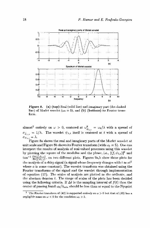
Figure 8. (a) (top) Real (solid line) and imaginary part (dot-dashed line) of Morlet wavelet (� � = 5), and (b) (bottom) its Fourier trans-form.
almost2 entirely on � > 0, centered at u°j — � � /� with a spread of = l /λ . The wavelet � � ^ itself is centered at t with a spread of � � � ,
� � � , = � . Figure 8a shows the real and imaginary parts of the Morlet wavelet at
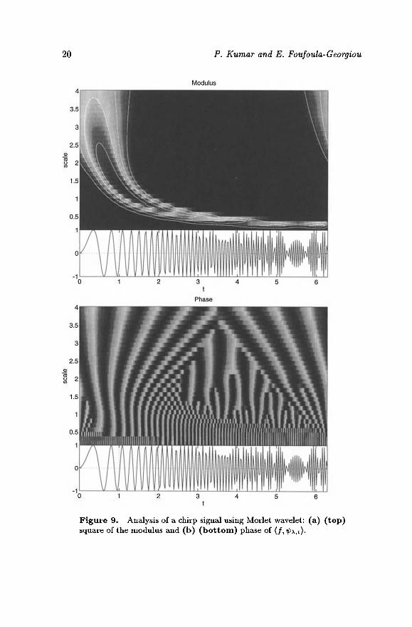
unit scale and Figure 8b shows its Fourier transform (with ωυ = 5 ) . One can interpret the results of analysis of real-valued processes using this wavelet by plotting the square of the modulus and the phase, i.e., | ( / , ip\, t)\2 and
on two different plots. Figures 9a,b show these plots for - 1 Im(f,il>xit) Re(f,tf>x,t) tan
the analysis of a chirp signal (a signal whose frequency changes with t as at2
where a is some constant). The wavelet transform was obtained using the Fourier transforms of the signal and the wavelet through implementation of equation (17). The scales of analysis are plotted as the ordinate, and the abscissa denotes t. The range of scales of the plots has been decided using the following criteria. If At is the sampling interval of f(t) then the center of passing band o;o/Amin should be less than or equal to the Nyquist
2 T h e Fourier t r ans fo rm of (42) is suppor t e d ent i re ly ο η ω > 0 b u t t h a t of (43) has a negligible m a s s o n w < 0 for t he condi t ion UJQ > 5.
Wavelet Analysis in Geophysics: An Introduction 19
frequency, i.e., o;o/Amin < 2π / 2Δί , implying
UlpAt Amin > . (45)
The maximum scale of analysis is obtained by considering the spread of ip\j. Recognizing tha t |^λ,ί | decays to 99.9% of its value at 3� � � t , we impose the condition 3σ^,λ f < (£m a x — £min) /2, i.e., the wavelet support should be contained within the da ta range, giving
(46) "Oiax *� � � �
The discretization of λ and t for implementation on discrete da ta is dis-cussed in the following sections.
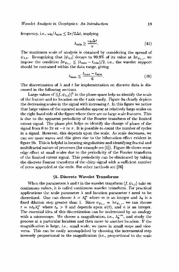
Large values of | ( / , � � ^)\2 in the phase-space help us identify the scale of the feature and its location on the t axis easily. Figure 9a clearly depicts the decreasing scales in the signal with increasing t. In this figure we notice tha t large values of the squared modulus appear at relatively large scales on the right hand side of the figure where there are no large scale features. This is due to the apparent periodicity of the Fourier transform of the limited extent signal. The phase plot helps us identify the change of phase of the signal from 0 to 2π or — � to π . It is possible to count the number of cycles in a signal. However, this depends upon the scale. As scale decreases, we can see more waves and this gives rise to the bifurcation effect evident in figure 9b. This is helpful in locating singularities and identifying fractal and multifractal na ture of processes (for example see [1]). Figure 9b shows some edge effect at small scales due to the periodicity of the Fourier transform of the limited extent signal. This periodicity can be eliminated by taking the discrete Fourier transform of the chirp signal with a sufficient number of zeros appended at the ends. For other methods see [26].
§5. D i scre te Wavele t Transforms
When the parameters λ and t in the wavelet transform (/ , � � ^) take on continuous values, it is called continuous wavelet transform. For practical applications the scale parameter λ and location parameter t need to be discretized. One can choose λ = λ™ where m is an integer and λ0 is a fixed dilation step greater than 1. Since � � � = \� � � , we can choose t = ntoX™ where to > 0 and depends upon ip(t), and n is an integer. The essential idea of this discretization can be understood by an analogy with a microscope. We choose a magnification, i.e., A^"m, and study the process at a particular location and then move to another location. If the magnification is large, i.e., small scale, we move in small steps and vice-versa. This can be easily accomplished by choosing the incremental step inversely proportional to the magnification (i.e., proportional to the scale
20 P. Kumar and E. Foufoula-Georgiou
Modulus
Phase
Figure 9. Analysis of a chirp signal using Morlet wavelet: (a) (top) square of the modulus and (b) (bottom) phase of (/, ip\,t).
Wavelet Analysis in Geophysics: An Introduction 21
\™) which the above method of discretization of t accomplishes. We then define
1 , , f - n t 0 A g \ � ™,� (*) = ~� ^� (—3^—)
ν Λ ο Λο = Ä 0 - m / V ( A 0 - m i - n i 0 ) . (47)
The wavelet transform
(/, t/>m,»> = \-m/2 J f(t)ip(\-mt - nt0) dt (48)
is called the discrete wavelet transform. In the case of the continuous wavelet transform we saw tha t (f, ip\ft)
for λ > 0 and t G (—οο,οο) completely characterizes the function f(t). In fact, one could reconstruct f(t) using (14). Using the discrete wavelet ipmin (with � decreasing sufficiently fast) and appropriate choices of λο and £o> we can also completely characterize f(t). In fact, we can write f(t) as a series expansion, as we shall see in the following subsections. We first s tudy orthogonal wavelets and then the general case.
5 .1 . Orthogonal wavelet transforms and mult ireso lut ion analys is
5 .1 .1 . Orthogona l wavelet transforms
Consider the discrete wavelet transform for λο = 2 and t0 = 1, i.e.,
i f ne}rri
</V» ( 0 = 2 - » / V ( 2 - r a t - n) = — � ( - ¥ — ) . (49)
For the purpose of this subsection, let ipm,n{t) denote the above discretiza-tion rather than the general discretization given by equation (47). We will also use the identity ^oo(^) = � (�)· It is possible to construct a certain class of wavelets ip(t) such tha t ipm,n(t) are orthonormal, i.e.,
/ · � � �,� (^)� � � ',� '(� dt = J m m / £ n n / (50)
where 6{j is the Kronecker delta function given as
%J \0 otherwise. ^ '
The above condition implies tha t these wavelets are orthogonal to their dilates and translates. One can construct ^ m ) „ ( i ) tha t are not only or-thonormal, but such tha t they form a complete orthonormal basis for all functions tha t have finite energy [30]. This implies tha t all such functions f(t) can be approximated, up to arbitrary high precision, by a linear com-
22 P. Kumar and E. Foufoula-Georgiou
bination of the wavelets ipmjn(t), i.e., oo oo
/(*)= � � Dm^m,n(t) (52) m= — oo n = —oo
where the first summation is over scales (from small to large) and at each scale we sum over all translates. The coefficients are obtained as
Dm,n = (�,� � �,� ) = I f ^)� m,� {1) dt
and, therefore, we can write oo oo
/(*)= � � (/^m,n)^m,„(i). (53) m— — oo n= — oo
From (53) it is easy to see how wavelets provide a time-scale representation of the process where time location and scale are given by indices n and m, respectively. The equality in equation (53) is in the mean square sense. The above series expansion is akin to a Fourier series with the following differences:
1. The series is double indexed with the indices indicating scale and location;
2. The basis functions have the time-scale (time-frequency) localization property in the sense discussed in section 2.2.
By using an intermediate scale mo, equation (53) can be broken up as two sums
oo oo mo oo
/ ( * ) = Σ Σ (�'� ™,� )� ,� ,� (*)+ Σ Σ </ '</>m,n>V>m,n(i) · m = m o + l n= — oo m— — con— — oo
(54) It turns out tha t one can find functions 0m )n(O defined analogous to
0m,n(i) = 2 - m / 2 0 ( 2 - m i - n ) (55) and satisfying certain properties enumerated in appendix A, such tha t the first sum on the RHS of equation (54) can be written as a linear combination of � � �� ,� (see [30]), i.e.,
oo oo oo
( ' ) = Σ Σ < / > ^ m , n ) t f m , n ( t ) · ( 5 6 ) � = — oo m = m o + l n = — oo
Consequently, oo m 0 oo
/ ( * ) = Σ < / , 4 > m „ , n > < £ m o , » W + Σ Σ < / > ^ m , n ) t f m , n ( t ) ( 5 7 ) n= — oo m=—oon= — oo
Wavelet Analysis in Geophysics: An Introduction 23
The function 0m,n(O is called a scaling function and satisfies J � (�) dt = 1 among its other properties. For example, the scaling function correspond-ing to the Haar wavelet is the characteristic function of the interval [0,1) given as
(58)
The scaling functions and wavelets play a profound role in the analysis of processes using orthogonal wavelets. This analysis framework is known as the wavelet multiresolution analysis framework and is discussed below. Ap-pendix B describes a class of orthogonal wavelets developed by Daubechies [13] and Appendix C briefly discusses the implementation algorithm by Mallat [30].
5.1.2. Multiresolution representat ion Equation (56) states that all the features of the process /(£), that are
larger than the scale 2m°, can be approximated by a linear combination of the translates (over n) of the scaling function <f)(t) at the fixed scale 2m°. Let us represent this approximation by PmQj', i.e.,
(59)
(60)
(61)
(62)
(63)
(64)
Let us now define
so that equation (57) becomes
Since mo is arbitrary we also have
from which we can obtain by subtraction
or in general
This equation characterizes the basic structure of the orthogonal wavelet decomposition (53). As mentioned before Pmf(t) contains all the informa-tion about features in f(t) that are larger than the scale 2m. From equation
24 P. Kumar and E. Foufoula-Georgiou
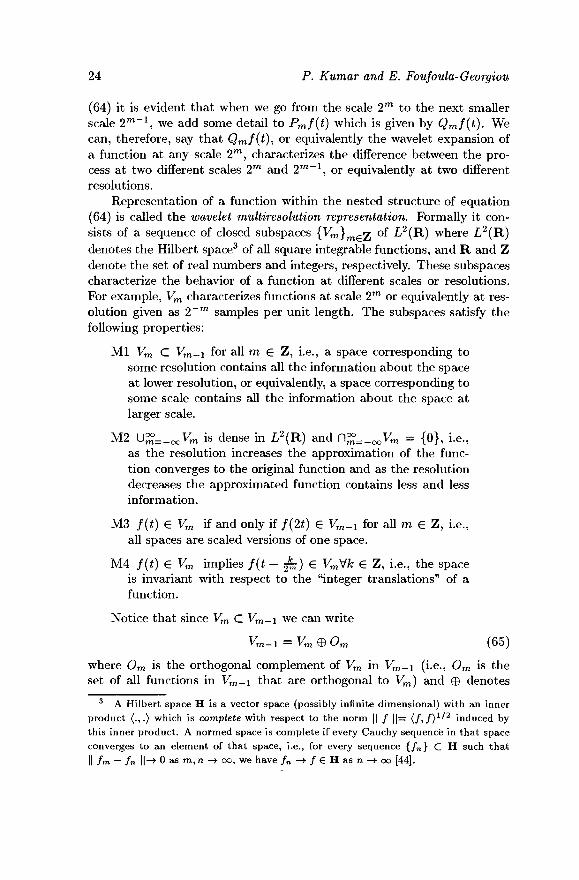
(64) it is evident tha t when we go from the scale 2 m to the next smaller scale 2 m _ 1 , we add some detail to Pmf(t) which is given by Qmf(t). We can, therefore, say tha t Q m / ( i ) , or equivalently the wavelet expansion of a function at any scale 2 m , characterizes the difference between the pro-cess at two different scales 2 m and 2 m _ 1 , or equivalently at two different resolutions.
Representation of a function within the nested structure of equation (64) is called the wavelet multiresolution representation. Formally it con-sists of a sequence of closed subspaces {Vr
m}m €2 °f L2(H) where L2(H) denotes the Hubert space3 of all square integrable functions, and R and Z denote the set of real numbers and integers, respectively. These subspaces characterize the behavior of a function at different scales or resolutions. For example, Vm characterizes functions at scale 2 m or equivalently at res-olution given as 2 _ m samples per unit length. The subspaces satisfy the following properties:
M l Vm C Vm-i for all m G Z, i.e., a space corresponding to some resolution contains all the information about the space at lower resolution, or equivalently, a space corresponding to some scale contains all the information about the space at larger scale.
M2 U^U.ooVm is dense in L 2 ( R ) and f l ^ . ^ V ^ = {0}, i.e., as the resolution increases the approximation of the func-tion converges to the original function and as the resolution decreases the approximated function contains less and less information.
M3 f(t) G Vm if and only if f(2t) G Vm_i for all m G Z, i.e., all spaces are scaled versions of one space.
M4 f(t) G Vm implies f(t - ^ r ) G VmVk G Z, i.e., the space is invariant with respect to the "integer translations" of a function.
Notice tha t since Vm C Vm-i we can write
Vm-i=Vm®Om (65)
where Om is the orthogonal complement of Vm in Vm_i (i.e., Om is the set of all functions in Vm-i tha t are orthogonal to Vm) and 0 denotes
3 A Hubert space H is a vector space (possibly infinite dimensional) with an inner product (.,.) which is complete with respect to the norm || / | |= (/, f)1/2 induced by this inner product. A normed space is complete if every Cauchy sequence in that space converges to an element of that space, i.e., for every sequence {/n} C H such that || fm — fn ||—y 0 as m, n -> oo, we have / „ - ^ / G H a s n - > o o [44].
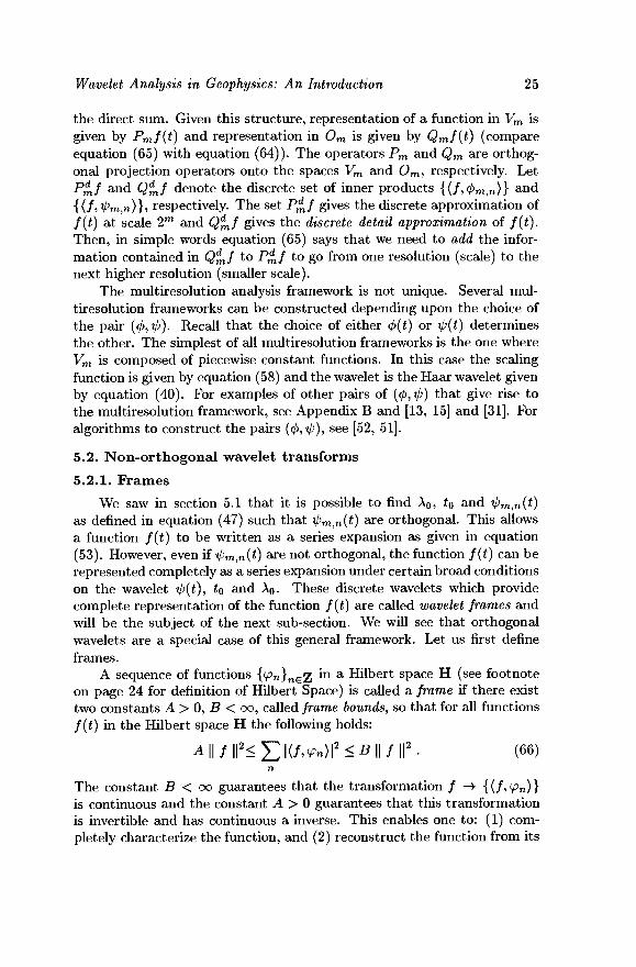
Wavelet Analysis in Geophysics: An Introduction 25
the direct sum. Given this structure, representation of a function in Vm is given by Pmf(t) and representation in 0m is given by Qmf(t) (compare equation (65) with equation (64)). The operators Pm and Qm are orthog-onal projection operators onto the spaces Vm and 0 m , respectively. Let P^f and Qmf denote the discrete set of inner products { ( / , </>m,n)} and {(�,� � �,� )}·, respectively. The set P^f gives the discrete approximation of f(t) at scale 2 m and Q^f gives the discrete detail approximation of f(t). Then, in simple words equation (65) says tha t we need to add the infor-mation contained in Q m / to P^f to go from one resolution (scale) to the next higher resolution (smaller scale).
The multiresolution analysis framework is not unique. Several mul-tiresolution frameworks can be constructed depending upon the choice of the pair (� ,� ). Recall tha t the choice of either � (�) or ip(t) determines the other. The simplest of all multiresolution frameworks is the one where Vm is composed of piecewise constant functions. In this case the scaling function is given by equation (58) and the wavelet is the Haar wavelet given by equation (40). For examples of other pairs of (� ,� ) t ha t give rise to the multiresolution framework, see Appendix B and [13, 15] and [31]. For algorithms to construct the pairs (� ,� ), see [52, 51].
5.2. N o n - o r t h o g o n a l wavelet transforms
5 .2 .1 . Frames
We saw in section 5.1 tha t it is possible to find λο, to and ipmin(t) as defined in equation (47) such tha t � � � ,� {�) are orthogonal. This allows a function f(t) to be written as a series expansion as given in equation (53). However, even if ^ m , n ( 0 are not orthogonal, the function f(t) can be represented completely as a series expansion under certain broad conditions on the wavelet r/>(i), t0 and λο· These discrete wavelets which provide complete representation of the function f(t) are called wavelet frames and will be the subject of the next sub-section. We will see tha t orthogonal wavelets are a special case of this general framework. Let us first define frames.
A sequence of functions {� � }� £� m a Hilbert space H (see footnote
on page 24 for definition of Hilbert Space) is called a frame if there exist two constants A > 0, B < oo, called frame bounds, so tha t for all functions f(t) in the Hilbert space H the following holds:
A | | / | | 2 < £ | < / , v > „ > l 2 < B | l / l l 2 · (66) n
The constant B < oo guarantees tha t the transformation / —> { ( / , � � ) } is continuous and the constant A > 0 guarantees tha t this transformation is invertible and has continuous a inverse. This enables one to: (1) com-pletely characterize the function, and (2) reconstruct the function from its
26 P. Kumar and E. Foufoula-Georgiou
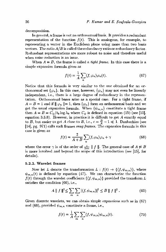
decomposition. In general, a frame is not an orthonormal basis. It provides a redundant
representation of the function f(t). This is analogous, for example, to representing a vector in the Euclidean plane using more than two basis vectors. The ratio A/B is called the redundancy ratio or redundancy factor. Redundant representations are more robust to noise and therefore useful when noise reduction is an issue.
When A = B, the frame is called a tight frame. In this case there is a simple expansion formula given as
� (�) = \� (� ,� � )� � {�). (67) n
Notice tha t this formula is very similar to the one obtained for an or-thonormal set {� � }· In this case, however, {� � } niay not even be linearly independent, i.e., there is a large degree of redundancy in the represen-tation. Orthonormal bases arise as a special case. For a tight frame, if A = B = 1 and if || � � \\= 1, then {� � } form an orthonormal basis and we get the usual expansion formula. When {^m,n} constitute a tight frame then A = B = C^ / io log^o where � � is defined in equation (15) (see [15], equation 3.3.8). However, in practice it is difficult to get A exactly equal to £?, but easier to get A close to B, i.e., e = -j — 1 <£ 1. Daubechies (see [14], pg. 971) calls such frames snug frames. The expansion formula in this case is given as
/ ( � ) = �� � � (/^>«+^ (68) n
where the error 7 is of the order of 2x7 || / ||· The general case of A 96 B is more involved and beyond the scope of this introduction (see [15], for details).
5.2 .2 . Wave le t frames
Now let L denote the transformation L : f(t) -l· {(/ , � � � , � )} , where tpm,n(t) is defined by equation (47). We can characterize the function f(t) through the wavelet coefficients { ( / , ipm,n)} provided the transform L satisfies the condition (66), i.e.,
� ||/� � 2<� � � />'/� »>� 2^� /� � 2· (69) m n
Given discrete wavelets, we can obtain simple expansions such as in (67) and (68), provided ^ m > n constitute a frame, i.e.,
W) = I � � </ ' VVn>̂ m,nW· (70) m n
Wavelet Analysis in Geophysics: An Introduction 27
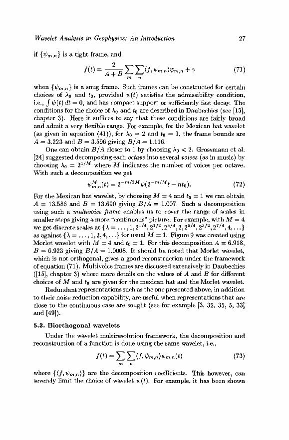
if {� � �,� } is a tight frame, and
/ ( � ) = � � � � � <·� ^>">^."+-� (7i) m n
when {� � �,� } is a snug frame. Such frames can be constructed for certain choices of λο and £o, provided ip(t) satisfies the admissibility condition, i.e., J � (�) dt — 0, and has compact support or sufficiently fast decay. The conditions for the choice of λο and to are described in Daubechies (see [15], chapter 3). Here it suffices to say tha t these conditions are fairly broad and admit a very flexible range. For example, for the Mexican hat wavelet (as given in equation (41)), for λο = 2 and to = 1, the frame bounds are A = 3.223 and B = 3.596 giving B/A = 1.116.
One can obtain B/A closer to 1 by choosing λο < 2. Grossmann et al. [24] suggested decomposing each octave into several voices (as in music) by choosing λο — 2 1 / / M where M indicates the number of voices per octave. With such a decomposition we get
� ™� (� = 2 - m / 2 A V ( 2 " m / M * - nto). (72)
For the Mexican hat wavelet, by choosing M = 4 and to = 1 we can obtain A = 13.586 and B = 13.690 giving B/A = 1.007. Such a decomposition using such a multivoice frame enables us to cover the range of scales in smaller steps giving a more "continuous" picture. For example, with M = 4 we get discrete scales at {λ = . . . , 1 , 2 1 / 4 , 2 1 / 2 , 2 3 / 4 , 2 , 2 5 / 4 , 2 3 / 2 , 2 7 / 4 , 4 , . . . } as against {λ = . . . , 1 ,2 ,4 , . . . } for usual M = 1. Figure 9 was created using Morlet wavelet with M = 4 and t0 = 1. For this decomposition A = 6.918, B = 6.923 giving B/A = 1.0008. It should be noted tha t Morlet wavelet, which is not orthogonal, gives a good reconstruction under the framework of equation (71). Multivoice frames are discussed extensively in Daubechies ([15], chapter 3) where more details on the values of A and B for different choices of M and to are given for the mexican hat and the Morlet wavelet.
Redundant representations such as the one presented above, in addition to their noise reduction capability, are useful when representations tha t are close to the continuous case are sought (see for example [3, 32, 35, 5, 33] and [49]).
5.3 . B ior thogona l wavele ts
Under the wavelet multiresolution framework, the decomposition and reconstruction of a function is done using the same wavelet, i.e.,
�(*) = � � (� ™.»)� ™.»� (73) m n
where { ( / , ^ m , n ) } are the decomposition coefficients. This however, can severely limit the choice of wavelet � (�). For example, it has been shown
28 P. Kumar and E. Foufoula-Georgiern
(see [15], theorem 8.1.4) tha t the only real and compactly supported sym-metric or antisymmetric wavelet under a multiresolution framework is the Haar wavelet. In certain applications however, real symmetric wavelets which are smoother and have bet ter frequency localization than the Haar wavelet may be needed. In such situations, biorthogonal wavelets come to the rescue. It is possible to construct two sets of wavelets {ipm^n} and {� � � ,� } such tha t
/(') = � � ^- .")</ � � ( � ) (74) m n
= EE</^™.»>^.«w· (75) m n
That is, one can accomplish decomposition using one set of wavelets and reconstruction using another. The wavelets ißmyn(t) = ^ 7 7 ^ ( 2 ^ — n ) a n ( ^
� � �,� ^) = 2^72^(2^ ~ n ) n e e d t 0 S a t i s fy
EEK/></Vn>|2 < B\\f\\* (76) m n
� � � /'Vw*)!2 ^ è\\f\\2 (77) m n
{� � �,� ,� � � ',� ') = ^mm'^nn' (78)
where B and B are some constants and condition (78) is the condition of biorthonormality. Given such a biorthonormal set, it is possible to con-struct corresponding scaling functions {� � �,� } a n d {<j>m,n} such tha t
\� � �,� ·)� � �,� '/ — ^� � '· v ' * V
Notice tha t nothing is said about the orthogonality of {� � � ,� }, {� � �,� }, {� � �,� } a n d {� � �,n) themselves. In general they form a linearly indepen-dent basis. Also, there is no condition of orthogonality between the wavelets � (�) and V>(£), a n d the corresponding scaling functions � (�) and 0(£), re-spectively. Given these wavelets and scaling functions, one can construct a multiresolution nest, as in the orthonormal case, i.e.,
• · · c v2 c Vi c v0 c y_i c K-2 c · · ·
• · · C V2 C Vi C Vo C VLi C V-2 C ■ ■ ■ with Vm — span{0 m j „} and Vm = span{0m > n } and the complementary spaces Om = span{^ m > n } and O m = s p a n { ^ m > n } . The spaces Vm and Om (Vm and O m , respectively) are not orthogonal complements in general. Equation (78), however, implies tha t
Vm JL Öm and Vm J- O m . (80)
Wavelet Analysis in Geophysics: An Introduction 29
Another advantage of biorthogonal wavelets is (see [15], section 8.3) tha t one can have ip(t) and zp(t) with different vanishing moments. For example, if ip(t) has more vanishing moments than � {�), one can obtain higher da t a compression using ( / , V>m,n) and a good reconstruction using
the sum being restricted to some finite values.
§6. Two-Dimens iona l Wave le t s
6 .1 . Cont inuous wavele ts
The continuous analogue of wavelet transform (12) is obtained by treat-ing u — (u 1,1*2) and t = (£1,^2) as vectors. Therefore for the two dimen-sional case
(81)
(82)
� > 0
An analogous inversion formula also holds, i.e.,
The condition of admissibility of a wavelet remains the same, i.e.,
1. compact support or sufficiently fast decay; and
2. fft{t)dt = 0. Two examples of two-dimensional wavelets are discussed in the follow-
ing subsection.
6 .1 .1 . Two-d imens iona l Morlet wavelet
Define the vector t = (£1,^2) on the two-dimensional plane with \t\ = \Jt\ -+-1\. Then the two dimensional Morlet wavelet is defined as
(83)
(84)
with Fourier transform
where Ω = {� \, � <� ) is an arbitrary point on the two-dimensional frequency plane, and Ω° = (ω^,ωί,) is a constant. The superscript � indicates the
30 P. Kumar and E. Foufoula-Georgiou
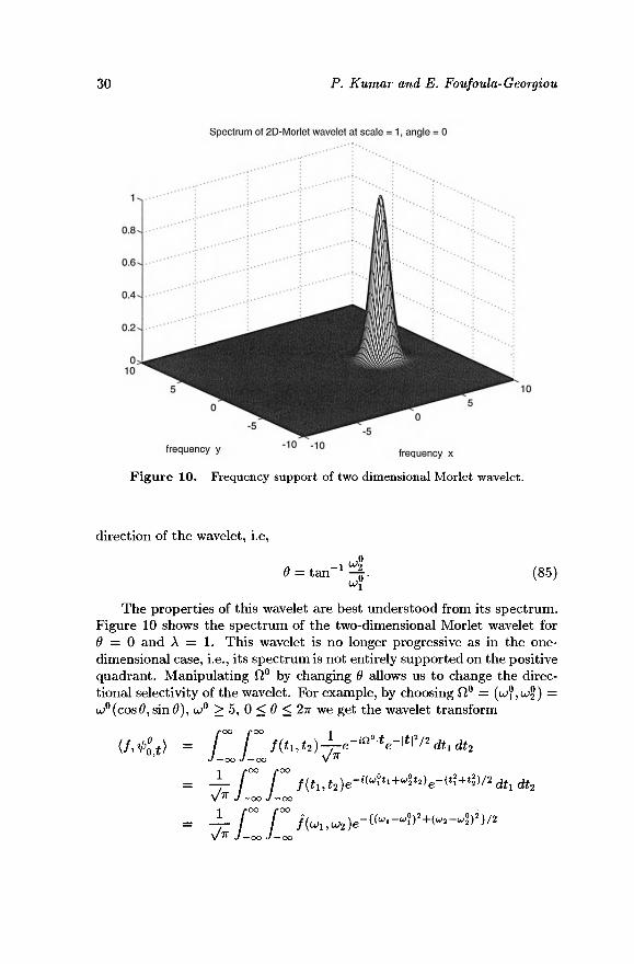
Figure 10. Frequency support of two dimensional Morlet wavelet.
direction of the wavelet, i.e,
^ t a n - 1 ^ . (85)
The properties of this wavelet are best understood from its spectrum. Figure 10 shows the spectrum of the two-dimensional Morlet wavelet for 0 = 0 and λ = 1. This wavelet is no longer progressive as in the one-dimensional case, i.e., its spectrum is not entirely supported on the positive quadrant . Manipulating Ω0 by changing � allows us to change the direc-tional selectivity of the wavelet. For example, by choosing Ω° = (ω?, � ^) = u;°(cos0,sin0), � ° > 5, 0 < � < 2π we get the wavelet transform
Wavelet Analysis in Geophysics: An Introduction 31
The last equation is obtained by using Parseval's theorem. At any arbitrary scale λ, equation (86) can be written as
\ /»OO /«OO 0 0
V^ J — OO J — OO
The above equation indicates tha t the wavelet transform {�,� �� *) extracts
the frequency contents of the function f(t) around the frequency coordi-nates (� �/� ,� ^/� ) = (� ° cos0/A,u;0 sin0/A) with a radial uncertainty of � ? = Ι /λ , at the location t. Therefore, by fixing λ and traversing along
0, directional information at a fixed scale λ can be extracted, and by fix-ing � and traversing along λ, scale information in a fixed direction can be obtained.
6.1 .2 . Halo wavelet
Often the directional selectivity offered by Morlet wavelet is not desired and one wishes to pick frequencies with no preferential direction. Dallard and Spedding [12] defined a wavelet by modifying the Morlet wavelet and called it the Halo wavelet because of its shape in the Fourier space. The wavelet itself is defined through its Fourier transform
� (� ) = � � -(� � � � °�>2/2 (88)
where n is a normalizing constant. As can be seen from the above expression this wavelet has no directional specificity.
6.2. Orthogona l wavele ts
For two-dimensional multiresolution representation, consider the func-tion / ( i i ,£2 ) £ I / 2 (R 2 ) . A multiresolution approximation of L 2 ( R 2 ) is a sequence of subspaces tha t satisfy the two-dimensional extension of prop-erties M l through M4 enumerated in the definition of the one-dimensional multiresolution approximation. We denote such a sequence of subspaces of L 2 ( R 2 ) by ( ^ m ) m G z · T k e a PP r o x i m a - t ion of the function / ( i i , Î 2 ) at the resolution m, i.e., 2 2 m samples per unit area, is the orthogonal projection on the vector space Vm.
A two-dimensional multiresolution approximation is called separable if each vector space Vm can be decomposed as a tensor product of two identical subspaces V^ of L 2 ( R ) , i.e., the representation is computed by filtering the signal with a low pass filter of the form Φ( ί ι , t2) = � (��)� ^2).
32 P. Kumar and E. Foufoula-Georgiou
For a separable multiresolution approximation of L 2 ( R 2 ) ,
Vm = t £ ® V £ (89)
where 0 represents a tensor product. It, therefore, follows (by expanding y m + i as in (89) and using property M l ) tha t the orthogonal complement 0m of Vm in Vm+\ consists of the direct sum of three subspaces, i.e.,
Om = {VL®Oln)®{Ol®V^)®{0]n®0]n). (90)
The orthonormal basis for Vm is given by
( 2 m * ( 2 m t i - n , 2 m t 2 - f c ) ) ( n fc)eZ2 = ( 2 m ^ m ( 2 m i 1 - n )^» m ( 2 m i 2 - f c ) ) ( n k ) ^ .
' <91> Analogous to the one-dimensional case, the detail function at the resolution m is equal to the orthogonal projection of the function on to the space Om
which is the orthogonal complement of Vm in V^+i . An orthonormal basis for Om can be built based on Theorem 4 in Mallat (1989a, pg. 683) who shows tha t if 4>{t\) ls the one dimensional wavelet associated with the scaling function � (�� ), then the three "wavelets" Φ 1 ^ , ^ ) — � (��)� (�2)·> Φ 2 ( ί ι , ί 2 ) = � {� )� {�2) and Φ 3 ( ί ι , ί 2 ) = � {� )� {�2) are such tha t
i V ^ m n / î ) ^ Trink") ^ m n k ) ( n k)£%2 J
is an orthonormal basis for Om. The discrete approximation of the function f(ti,t2) at a resolution m
is obtained through the inner products
Pif = {(f,*rnnk)(nk)€Z*} = { ( / . 0 π ,η ^ » * ) (Μ ) 6 Ζ » } (92)
The discrete detail approximation of the function is obtained by the inner product of / ( i i ,£2) with each of the vectors of the orthonormal basis of Om. This is, thus, given by
Ä 7 = {(/,*L,*)(n,fc)<Ez2}> (93)
Ä 2 / = {(/,*L,*)(„,fc)€z*K (94) and
Q£/ = {(/,*3m„*)(n,fc)€Z'}· (95)
The corresponding continuous approximation will be denoted by Qmf(t), Qmf(t) and Qmf(t) respectively. For implementation to discrete da ta see [31]·
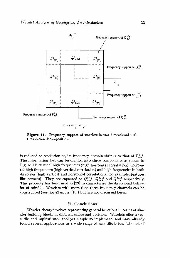
The decomposition of Om into the sum of three subspaces (see equa-tion (90)) acts like spatially oriented frequency channels. Assume tha t we have a discrete process at some resolution m + 1 whose frequency domain is shown in Figure 11 as the domain of Pm+if. When the same process
Wavelet Analysis in Geophysics: An Introduction 33
� 3
� 2 � � (� )
� 3 � 3(� )
Frequency support of Pmf
� 1 � (� )
Ψ (ω)
Frequency support of Q mf
� 3
� 2
� 3
Frequency support of Q ^2f
Frequency support of P f
.Frequency support of Q mf
� = ( œt , cot ) 1 2
Figure 11 . Frequency support of wavelets in two dimensional mul-tiresolution decomposition.
is reduced to resolution ra, its frequency domain shrinks to tha t of P^f. The information lost can be divided into three components as shown in Figure 11: vertical high frequencies (high horizontal correlation), horizon-tal high frequencies (high vertical correlation) and high frequencies in bo th direction (high vertical and horizontal correlations, for example, features like corners). They are captured as Q ^ / , Q^f a n d Qmf respectively. This property has been used in [29] to characterize the directional behav-ior of rainfall. Wavelets with more than three frequency channels can be constructed (see, for example, [10]) but are not discussed herein.
§7. Conclus ions
Wavelet theory involves representing general functions in terms of sim-pler building blocks at different scales and positions. Wavelets offer a ver-satile and sophisticated tool yet simple to implement, and have already found several applications in a wide range of scientific fields. The list of

34 P. Kumar and E. Foufoula-Georgiou
Table I Anonymous ftp site information for wavelet related software.
1 FTP site cs.nyu.edu playfair.stanford.edu simplicity.stanford.edu gdr.bath.ac.uk pascal.math.yale.edu
[email protected] cml.rice.edu
1 wuarchive.wustl.edu
Directory pub/wave pub/software/wavelets /pub/taswell /pub/masgpn /pub/software/xwpl
e-mail request /pub/dsp/software edu/math/msdos/modelling
References/Notes f [35, 33], C programs 1 MATLAB Scripts MATLAB scripts S software Wavelet Packet Laboratory for KHOROS MATLAB scripts C programs
wavelet applications increases at a fast pace and includes to date signal pro-cessing, coding, fractals, statistics, image processing, astrophysics, physics, turbulence, mathematics, numerical analysis, economics, medical research, target detection, industrial applications, quantum mechanics, geophysics etc. (see, for example, the edited volumes by Chui [7], Ruskai et al. [48], Benedetto and Frazier [3], Farge et al. [20], Meyer and Roques [41], Combes et al. [9], and Beylkin et al. [2], among others). A general li terature survey on wavelets can be found in [46]. In geophysics, significant progress has already been made in studying and unraveling structure of several geophys-ical processes using wavelets (see the extended bibliography of wavelets in geophysics at the end of this volume). We have no doubt tha t the study of geophysical phenomena, which are by nature complex, and take place and interact at a range of scales of interest, will continue to benefit from the use of the powerful and versatile tools tha t wavelet analysis has to offer.
There are a number of useful sources of information about wavelet pub-lications and computer software for the implementation of wavelet analysis. An electronic information service called "wavelet digest" exists (at the t ime of this writing) on the Internet with the address waveletumath.scarolina.edu. Several anonymous ftp sites exist on the Internet from where software for wavelet analysis can be obtained. In Table I we provide a brief list (known to the authors at the time this was written) solely for the purpose of infor-mation to readers, without any recommendations, or reference to suitability or correctness of these codes.
A. Propert i e s of Scaling Funct ion
The scaling function satisfies the following properties:
1. j 4>(t)dt = 1, i.e., the scaling function is an averaging function-, compare this with the wavelet tha t satisfies / � (�) dt = 0.
Wavelet Analysis in Geophysics: An Introduction 35
2. || � (�) | |= 1, i.e., the scaling function is normalized to have unit norm.
3. f � � � ,� (�)� � �',� '(t) dt = 0, i.e., the scaling function is orthogonal to all the wavelets.
4. j ' � � � ,� (�)� � �,� '(�) dt = Snn>, i.e., the scaling function is orthogonal to all its translates at any fixed scale. Note tha t unlike the wavelets, the scaling function is not orthogonal to its dilates. In fact,
5. (j)(t) = � � ��(� )� (2� — � ), i.e., the scaling function at some scale can be obtained as a linear combination of itself at the next scale (h(n) are some coefficients called the scaling coefficients). This is a two-scale difference equation (see [16] and [17] for a detailed t reatment of such equations).
6. The scaling function and wavelet are related to each other. In fact, one can show tha t
� {�) = � /9{� )� {2�-� ) (A.l) n
where g(n) are coefficients derived from h(n). Tha t is, the wavelets can be obtained as a linear combination of dilates and translates of the scaling function.
For the particular case of Haar wavelet (see equation (40)) and the corre-sponding scaling function (equation (58)) h(0) = h(l) = 1 and h{n) = 0 for all other n, and g(l) = —g(0) = 1 and g(n) = 0 for all other n.
B . Daubech ie s ' Wave le t s
Daubechies [13] developed a class of compactly supported scaling func-tions and wavelets denoted as ( ^ , � /� ). They were obtained through the solution of the following two-scale difference equations:
2N-1
� (� = y/2 � � � )� {2� - n) (� ·�)
2ΛΓ - 1
tl>(t) = j2 � 9{� )� {2�-� ) (Β.2) n=0
where g(n) = (-l)nh(2N - n + 1) for n = 0 , 1 , . . . , 2N - 1. (B.3)
For techniques to solve the above equations see [52]. The scaling coefficients h(n) are obtained from solutions of high order polynomials ([15], chapter 6, and [51]) and satisfy the following constraints:
36 P. Kumar and E. Foufoula-Georgiou
1. A necessary and sufficient condition for the existence of a solution to the above two-scale difference equations is
2ΛΓ - 1
� M») = \/2· (� .4) n=0
2. Integer translations and dilations of </>(£) and � (�) form an orthog-onal family if the scaling coefficients satisfy
2 J V - 1
J2 h(n - 2k)h(n - 21) = Skl for all k and I. (B.5) n=0
3. The constraints 2 7 V - 1
� {-l)n~lnkh{n) = 0 for k = 0 , 1 , . . . , N - 1 (B.6)
yield the result tha t � (�) has N vanishing moments, i.e.,
tktp(t) at = 0 for k = 0 , 1 , . . . , N - 1. (B.7) /�
Daubechies' wavelets of this class have the following properties:
1. They are compactly supported with support length 2N — 1. The scaling function also has the same support length.
2. As iV increases, the regularity of � � and � � also increases. In fact � � ,� � £ CaN (the- set of continuous functions tha t are a^ order differential) where (iV, α^γ) pairs for some iV are given as (see [13])
{(2,0.5 - e), (3,0.915), (4,1.275), (5,1.596), (6,1.888), (7,2.158)}.
3. Condition (B.7) of vanishing moments of � (�) implies tha t up to Nth order derivatives of the Fourier transform of � (�) at the origin are zero, i.e.,
-^� ^� = 0) = 0 for k = 0 , 1 , . . . , iV - 1. (B.8)
This property essentially implies a form of localization of the Fourier transform � (� ).
Figures B l and B2 show the scale function and the corresponding wavelets for N = 2 and TV = 5 respectively. The figures also depict the magnitude of their Fourier transforms. As can be seen the regularity of the wavelets and the scale functions increase as N increases.
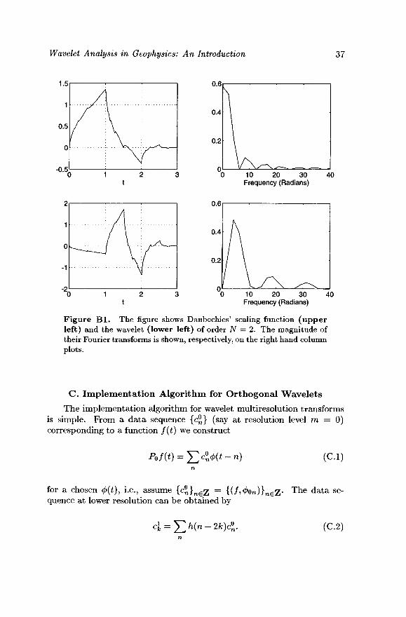
Wavelet Analysis in Geophysics: An Introduction 37
10 20 30 Frequency (Radians)
40
10 20 30 Frequency (Radians)
40
Figure B l . The figure shows Daubechies' scaling function (upper left) and the wavelet (lower left) of order N = 2. The magnitude of their Fourier transforms is shown, respectively, on the right hand column plots.
C. I m p l e m e n t a t i on Algor i thm for Orthogonal Wave le t s
The implementation algorithm for wavelet multiresolution transforms is simple. From a da ta sequence {c^} (say at resolution level m = 0) corresponding to a function f(t) we construct
� „/(*) = � <£#'-") (C.I)
for a chosen <£(£), i.e., assume { c ° } n €£ = { ( / ,0On)} n G z · The da ta se-quence at lower resolution can be obtained by
ci = 5>(»-2*)<$. (C.2)
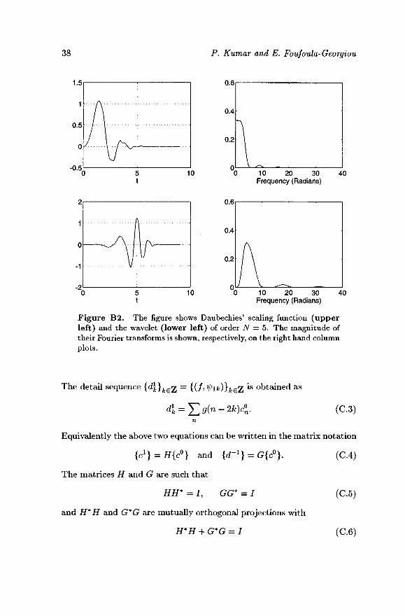
38 P. Kumar and E. Foufoula-Georgiou
10 20 30 Frequency (Radians)
10 20 30 Frequency (Radians)
40
40
Figure B2. The figure shows Daubechies' scaling function (upper left) and the wavelet (lower left) of order N = 5. The magnitude of their Fourier transforms is shown, respectively, on the right hand column plots.
The detail sequence {^}f c Gz = {(/ '^i^)}fceZ 1S obtained as
d\ = Y,g{n-2k)cl (C.3)
Equivalently the above two equations can be written in the matr ix notat ion
{c1} = H{c0} and {d" 1 } = G{c 0 } . (C.4)
The matrices H and G are such tha t
HH* = / , GG* = I (C.5)
and H*H and G*G are mutually orthogonal projections with
H*H + G*G = I (C.6)
Wavelet Analysis in Geophysics: An Introduction 39
where H* and G* are adjoints of H and G respectively and i" is the identity matrix. Also,
GH* = 0 and HG* = 0. (C.7)
The algorithm given in equation (C.2) and (C.3) can be recursively im-plemented and the da ta and details at lower and lower resolutions can be obtained. This also highlights another important feature. Once we have the coefficients h{n), we never need to construct the scale function 0(f) or the wavelet � (�) for implementation on a discrete da ta set. The assump-tion involved, however, is tha t c^ = f f(t)(f)(t — n)dt, i.e., the integration kernel is � (�) corresponding to the chosen /i(n)'s. The reconstruction of the original sequence can be achieved by using
c™-1=2Y^h(n-2k)cÎ + 2j2g(n-2k)dZ (C.8) k k
and is exact.
R e f e r e n c e s
1. Arneodo, A., G. Grasseau and M. Holschneider, Wavelet transform of multifractals, Physical Rev. Let, 61(20), 2281-2284, 1988.
2. Beylkin, G., R. R. Coifman, I. Daubechies, S. G. Mallat, Y. Meyer, L. A. Raphael, M. B. Ruskai (eds.), Wavelets and Their Applications, Jones and Bartlet t Publishers, Boston, 1991.
3. Benedetto J. J., and M. W. Frazier (eds.), Wavelets: Mathematics and Applications, CRC Press, Boca Raton, Florida, 1993.
4. Brunet , Y. and S. Collineau, Wavelet analysis of diurnal and nocturnal turbulence above a maize crop, This Volume, 1994.
5. Burt , P. J., Fast filter transforms for image processing, Computer Graphics and Image Processing, Vol. 16, 20-51, 1981.
6. Chui, C. K., An Introduction to Wavelets, Wavelet Analysis and its Applications, Vol. 1, Academic Press, New York, 1992.
7. Chui, C. K., Wavelets - a Tutorial in Theory and Applications, Wavelet Analysis and its Applications, Vol. 2, Academic Press, New York, 1992.
8. Coifman, R. R., Y. Meyer and V. Wickerhauser, Size properties of wavelet-packets, in Ruskai et al., 453-470, 1992.
9. Combes, J. M., A. Grossman, Ph. Tchamitchian (eds.), Wavelets: Time-Frequency Methods and Phase-Space, Proc. of the Int. Conf., Marseille, Frace, Decemberl4-18, 1987, Springer-Verlag, 1989.
10. Cohen, A., Non-separable bidimensional wavelet bases, Revista Mathematica Iberoamericana, 9(1), 51-137, 1993.
11. Cohen, L., Time-frequency distributions-a review, Proc. of the IEEE, 77(7), 941-981, 1989.
40 P. Kumar and E. Foufoula-Georgiou
12. Daliard, T. and G. R. Spedding, 2-D wavelet transforms, Preprint, 1990.
13. Daubechies, L, Orthonormal bases of compactly supported wavelets, Commun, on Pure and Appl. Math., Vol. XLI, 901-996, 1988.
14. Daubechies, I., The wavelet transform, time-frequency localization and signal analysis, IEEE Trans. Info. Theory, 36(5), 1990.
15. Daubechies, I., Ten Lectures on Wavelets, SIAM, 1992. 16. Daubechies, I. and J. C. Lagarias, Two-scale difference equations I. ex-
istence and global regularity of solutions, SIAM J. Math. Anal., 22(5), 1388-1410, 1991.
17. Daubechies, I. and J. C. Lagarias, Two-scale difference equations II. local regularity, infinite products of matrices and fractals, SIAM J. Math. Anal., 23(4), 1031-1079, 1992.
18. Daubechies, I., Review of the Books: Wavelets and Operators, Y. Meyer, (Cambridge University Press, New York, 1993, Cambridge Studies in Advanced Mathematics, 37, Translation from the french edition, Paris, 1990, by D.H. Salinger) and Wavelets: Algorithms and Applications, Y. Meyer, (SIAM, Philadelphia, 1993, Translation form the french edition, by R. D. Ryan), Science, 262, 1589-1591, 1993.
19. Farge, M., Wavelet transforms and their applications to turbulence, Annu. Rev. Fluid Mech., 24, 395-457, 1992.
20. Farge, M., J. R. Hunt, J. C. Vassilicos (eds.), Wavelets, Fractals and Fourier Transforms: New Developments and New Applications, Oxford University Press, Oxford, 1991.
21. Flandrin, P., Time-frequency and time-scale, IEEE Fourth Annual ASSP Workshop on Spectrum Estimation and Modeling, Minneapolis, Minnesota, 77-80, 1988.
22. Gabor, D., Theory of communications, J. Inst. Elec. Eng., Vol. 93, 429-457, 1946.
23. Goupillaud, P., A. Grossmann and J. Morlet, Cycle-octave and related transforms in seismic signal analysis, Geoexploration, 23, 85-102, 1984.
24. Grossmann, A. and J. Morlet, Decomposition of Hardy functions into square integrable wavelets of constant shape, SIAM J. math. Anal. 15(4), 723-736, 1984.
25. Hudgins L. H., M. E. Mayer and C. A. Friehe, Fourier and wavelet analysis of atmospheric turbulence, in Progress in Wavelet Analysis and Applications, Y. Meyer and S. Roques, eds., 491-498, Editions Frontiers, 1993.
26. Jawerth, B, and W. Sweldens, An overview of wavelet based multires-olution analyses, to appear, SIAM review, 1994.
27. Katul , G. G., J. D. Albertson, C. R. Chu, and M. B. Parlange, Inter-mittency in atmospheric turbulence using orthonormal wavelet, This Volume, 1994.
Wavelet Analysis in Geophysics: An Introduction 41
28. Kumar, P. and E. Foufoula-Georgiou, A multicomponent decomposi-tion of spatial rainfall fields: 1. segregation of large and small-scale features using wavelet transforms, Water Resour. Res., 29(8), 2515-2532, 1993.
29. Kumar, P. and E. Foufoula-Georgiou, A multicomponent decomposi-tion of spatial rainfall fields: 2. self-similarity in fluctuations, Water Resour. Res., 29(8), 2533-2544, 1993.
30. Mallat, S., A theory for multiresolution signal decomposition: the wavelet representation, IEEE Tran, on Pattern Anal, and Mach. Intel., 11(7), 674-693, 1989.
31. Mallat, S, Multifrequency channel decomposition of images and wavelet models, IEEE Trans, on Acoustics, Speech and Signal Anal. 37(12), 2091-2110. Dec. 1989.
32. Mallat, S., Zero-crossings of a wavelet transform, IEEE Trans. Inform. Theory, 37(4), 1019-1033, 1991.
33. Mallat, S. and L. Hwang, Singularity detection and processing with wavelets, IEEE Trans. Inform. Theory, 38(2), 617-643, 1992.
34. Mallat, S. and S. Zhong, Wavelet transform maxima and multiscale edges, in Wavelets and Their Applications, M. B. Ruskai, G. Beylkin, R. Coifman, I. Daubechies, S. Mallat, Y. Meyer, L. Raphael, eds., Jones and Bart let t , Boston, 1992.
35. Mallat, S. and S. Zhong, Complete signal representation from multi-scale edges, IEEE Trans. Pattern Anal. Machine Intell, 14(7),710-732, 1992.
36. Meneveau, C., Analysis of turbulence in the orthonormal wavelet rep-resentation, J. Fluid Mech., 332, 469-520, 1991.
37. Meyer, Y., Ondolettes et applications, J. Annu. Soc. Math., Soc. Fran-çaise Math. , Paris, France, pp. 1-15., 1990.
38. Meyer, Y., Wavelets and Operators, (Translation from the French Edi-tion, Paris, 1990, by D. H. Salinger) Cambridge University Press, New York, 1993, Cambridge Studies in Advanced Mathematics , 37.
39. Meyer, Y., Wavelets: Algorithms and Applications, SI AM, Philadel-phia, 1993.
40. Meyer, Y., Review of Books An introduction to wavelets by C. K. Chui, and Ten Lectures on Wavelets by I. Daubechies, Bulletin (New Series) of the American Mathematical Society, 28(2), 350-360, 1993.
41. Meyer, Y. and S. Roques (eds.), Progress in Wavelet Analysis and Applications, Editions Frontieres, France, 1993.
42. Morlet, J., G. Arens, E. Fourgeau, and D. Giard, Wave propogation and sampling theory- par t 1: complex signal and scattering in multilayered media, Geophysics, 47(2), 203-221, 1982.
43. Morlet, J., G^ Arens, E. Fourgeau, and D. Giard, Wave propogation and sampling theory- part 2: sampling theory and complex waves,
42 P. Kumar and E. Foufoula-Georgiou
Geophysics, 47(2), 222-236, 1982. 44. Naylor, A. W. and G. R. Sell, Linear Operator Theory in Engineering
and Science, Springer-Verlag, New York, 1982. 45. Pike, C. J., Analysis of high resolution marine seismic data using the
wavelet transform, This Volume, 1994. 46. Pittner, S., J. Schneid, and C. W. Ueberhuber, Wavelet Literature
Survey, Institute for Applied and Numerical Mathematics, Technical University Vienna, Wien, Austria, 1993.
47. Rioul, 0 . and M. Vetterli, Wavelets and signal processing, IEEE Signal Processing Magazine, 14-38, Oct. 1991.
48. Ruskai, M. B., G. Beylkin, R. Coifman, I. Daubechies, S. Mallat, Y. Meyers, and L. Raphael (eds.), Wavelets and Their Applications, Jones and Bartlett Publishers, 1992.
49. Saito, N. and G. Beylkin, Multiresolution representations using the auto-correlation functions of compactly supported wavelets, IEEE Trans, on Signal Processing, 41(12), 3584-3590, 1993.
50. Saito, N., Simultaneous noise suppression and signal compression using a library of orthonormal bases and the minimum description length criterion, This volume, 1994.
51. Strichartz, R. S., How to make wavelets, The Amer. Mathematical Monthly, 100(6), 539-556, 1993.
52. Strang, G., Wavelets and dilation equations: a brief introduction, SIAM Rev., 31(4), 614-627, 1989.
53. Wickerhauser, V., Lectures on wavelet packets algorithms, Preprint, Dept. of Math., Washington Univ., 1991.
The first author would like to thank Mike Jasinski and the Hydrologie Sciences Branch at NASA-Goddard Space Flight Center for the support during the course of this work. The second author would like to acknowl-edge the support of National Science Foundation grants BSC-8957469 and EAR-9117866, and NASA grant NAG 5-2108. We would also like to ac-knowledge the thoughtful comments of Don Per ci val, Naoki Saito and Paul Liu on this chapter.
Praveen Kumar Universities Space Research Association/ Hydrological Sciences Branch (Code 974) NASA-Goddard Space Flight Center Greenbelt, MD 20771 [email protected]
Wavelet Analysis in Geophysics: An Introduction 43
Efi Foufoula-Georgiou St. Anthony Falls Hydraulic Laboratory Department of Civil and Mineral Engineering University of Minnesota Minneapolis, Minnesota 55414 e-mail: efiUmykonos.safhl.umn.edu