Wavelet-Based Parameter Estimation for TrendContaminated Fractionally Differenced Processes

Peter F. Craigmile Donald B. Percival Peter Guttorp

NRCSET e c h n i c a l R e p o r t S e r i e s

NRCSE-TRS No. 047

May 30, 2000

The NRCSE was established in 1996 through a cooperative agreement with the United StatesEnvironmental Protection Agency which provides the Center's primary funding.

Wavelet-Based Parameter Estimation for Trend

Contaminated Fractionally Di�erenced Processes

Peter F. Craigmile, 1 Donald B. Percival 2;3 and Peter Guttorp 1.

1Department of Statistics, Box 354322, University of Washington, Seattle. WA 98195{4322.

2Applied Physics Laboratory, Box 355640, University of Washington, Seattle. WA 98195{5640.

3MathSoft Inc., 1700 Westlake Avenue North, Suite 500, Seattle. WA 98109{3044.

Correspondence Address:

Peter F. Craigmile,

Department of Statistics,

Box 354322,

University of Washington,

Seattle. WA 98195{4322.

1

Wavelet-Based Parameter Estimation for Trend

Contaminated Fractionally Di�erenced Processes

Peter F. Craigmile, 1 Donald B. Percival 2;3 and Peter Guttorp 1.

Last updated May 30, 2000.

1Department of Statistics, Box 354322, University of Washington, Seattle. WA 98195{4322.

2Applied Physics Laboratory, Box 355640, University of Washington, Seattle. WA 98195{5640.

3MathSoft Inc., 1700 Westlake Avenue North, Suite 500, Seattle. WA 98109{3044.

Abstract:

A common problem in the analysis of time series is how to deal with a possible trend component,

which is usually thought of as large scale (or low frequency) variations or patterns in the series

that might be best modelled separately from the rest of the series. Trend is often confounded

with low frequency stochastic uctuations, particularly in the case of models such as fractionally

di�erenced (FD) processes, which can account for long memory dependence (slowly decaying auto-

correlation) and can be extended to encompass non-stationary processes exhibiting quite signi�cant

low frequency components. In this paper we assume a model of polynomial trend plus FD noise

and apply the discrete wavelet transform (DWT) to separate a time series into pieces that can be

used to estimate both the FD parameters and the trend. The estimation of the FD parameters is

based on an approximate maximum likelihood approach that is made possible by the fact that the

DWT decorrelates FD processes approximately. We demonstrate our methodology by applying it

to a popular climate dataset.

Keywords: fractionally di�erenced processes; discrete wavelet transform; trend; limit distribution;

con�dence intervals.

2

1 Introduction

In recent years long memory processes have been used to model natural phenomena in areas such as

atmospheric sciences, geosciences and hydrology. Such processes are characterised by slowly decaying

autocorrelations which can be hard to model using short term models such as the auto-regressive

moving average (ARMA) class of models (Box, Jenkins, and Reinsel (1994)). One common example

of a long memory process, the fractionally di�erenced (FD) process (Granger and Joyeux (1980),

Hosking (1981)), extends existing (integer) integrated processes. The succinct de�nition of an FD

process in terms of its spectral density function allows for a varied range of estimation methods.

Considering the FD process singly, a common method of parameter estimation involves calculating

the exact likelihood and maximising with respect to the parameters. Beran (1994) gives a review and

evaluation of this. He concludes that two factors hampering such methods in practice are (1) slow

computations (a consideration that is becoming less and less important with current technology) and

(2) inaccuracies due to a large number of computations. The second can be a signi�cant problem in

this framework because the matrix calculations involved are O(N2). Various approximate likelihood

methods have been proposed to overcome this (Beran (1994)). Some of these methods exploit

fast transforms of the data such as the FFT (Robinson (1994)) or wavelet transforms (Wornell

(1995), McCoy and Walden (1996)). Jensen (2000) considers a wavelet method for estimation of

auto-regressive, fractionally integrated, moving average (ARFIMA) processes.

There is less literature in the case of such a process being contaminated by a trend component. The

topic of long-range dependence and trends is dealt with in Smith (1989a), Smith (1989b) and Smith

(1993). Teverovsky and Taqqu (1997) consider tests for long memory dependence in the presence

of two types of trend (shifting means and slowly decaying trend). Percival and Bruce (1998) extend

the wavelet based approximate likelihood estimates of McCoy and Walden (1996) to work in the

presence of polynomial trends. Beran (1999) uses variable bandwidth smoothing to estimate such

processes with additive trend.

In this paper we consider estimation of the parameters of a trend contaminated FD process using

the discrete wavelet transform (DWT). Wavelet transforms of such time series are useful because:

1. They approximately de-correlate FD and related processes. We will show the resulting wavelet

3

coeÆcients form a near independent Gaussian sequence, simplifying the statistics signi�cantly;

2. Wavelets have excellent time and frequency localisation, which can be useful for expressing

local deviations from a statistical model;

3. Wavelets can separate certain non-linear trends from noise, thus allowing us to analyse depen-

dent time series with a trend.

In this paper we concentrate on polynomial trends, but it is easy using the �nal two properties to

extend these results to other smooth and non-smooth trends (see Craigmile, Percival, and Guttorp

(2000a) for further details on this).

By using the wavelet coeÆcients of the transform in a multivariate Gaussian model (with an assumed

simpli�ed correlation structure of the coeÆcients), we can estimate the parameters using maximum

likelihood. In particular we consider two models:

� White noise wavelet model - we assume the wavelet coeÆcients are independent both within

and across wavelet scales;

� AR(1) wavelet model. We show that there is often a small lag-one auto-correlation between

wavelet coeÆcients on a speci�c scale. As an approximation to this we assume independence

across scales, and an AR(1) model per each wavelet scale.

We consider limits theorem and approximate con�dence intervals for the parameters in these models,

and Monte Carlo simulations are used to assess these methods. We end by applying the theory to a

northern hemisphere temperature dataset obtained from the Climate Research Unit, University of

East Anglia, UK.

2 The Discrete Wavelet Transform

Suppose X = (X0 : : : XN�1) is the observed time series with N divisible by 2J for some integer

J . For an even integer L, let fhlgL�1l=0 denote a Daubechies (Daubechies (1992)) wavelet �lter. By

de�nition this �lter has a square gain function given by

H1(f) � 2 sinL(�f)PL

2�1

l=0

�L2�1+ll

�cos2l(�f): (1)

4

Note that the square gain function does not uniquely specify the wavelet �lter. Daubechies distin-

guishes between two types:

� The extremal phase, D(L), �lters are the ones which exhibit the smallest delay (have maximum

cumulative energy) over other choices of wavelet �lter;

� The least asymmetric, LA(L), �lters are de�ned for L=8,10,. . . . These �lters are closest to

that of a linear phase �lter.

We refer to the D(2) wavelet as the Haar wavelet for historical reasons. All these wavelet �lters are

useful because they can reduce polynomials to zero due to an inherent di�erencing in the �lter.

Corresponding to the �lter we let W denote a N � N orthonormal DWT matrix of level J . The

DWT coeÆcients are then given by W =WX. We partition these coeÆcients as

W = (W1;W2; : : : ;WJ ;VJ )

� Wj are the N=2j wavelet coeÆcients associated with changes in average on scale �j � 2j�1

and with times spaced �j � 2j units apart;

� VJ are the N=2J scaling coeÆcients associated with averages on scale �J � 2J�1 and with

times spaced �J � 2J units apart.

Equivalent to the matrix form, the \pyramid algorithm" (Mallat (1989)) can be used to calculate

W hierarchically (see e.g. Percival and Walden (2000) for a step-by-step guide to this algorithm).

Letting Lj � (2j � 1)(L � 1) + 1, the jth level wavelet coeÆcients can also be computed using the

jth level wavelet �lter fhj;lgLj�1l=0 :

Wj;k =

Lj�1Xl=0

hj;lX2j(k+1)�l�l mod Nj�1j = 1 : : : J; k = 0 : : : Nj � 1

where fhj;lg has a square gain function given by

Hj(f) � H1(2j�1f)

j�2Yk=0

H1(12 � 2kf): (2)

5

The DWT handles �ltering operations periodically. That is to say a number of the wavelet coeÆ-

cients on each level are a weighted sum of points at the start and the end of the original signal. In

particular the �rst Bj � d(L�2)(1�2�j )e wavelet coeÆcients are a�ected by this circularity problem.

We call these coeÆcients the boundary dependent coeÆcients. The remainingMj � N=2j�Bj are un-

a�ected by boundaries and are named the boundary independent coeÆcients. We let M �PJj=1Mj

denote the total number of boundary-independent wavelet coeÆcients. As we shall see the statistical

properties of the two sets of wavelet coeÆcients are very di�erent.

3 Fractionally Di�erenced Processes

The fractionally di�erenced (FD) process is an example of a long memory dependence model in

which the covariance fades slowly over increasing lags. The process was originally proposed by

Granger and Joyeux (1980) and Hosking (1981) as an extension to ARIMA(0; d; 0) models to allow

for fractional values of d.

De�nition 3.1 Let d 2 [�1=2; 1=2) and �2� > 0. We say that fXtgt2Z is a FD(d; �2� ) or

ARFIMA(0; d; 0) process if it has spectral density function:

SX(f) = �2� j2 sin(�f)j�2d for jf j � 1=2: (3)

d is known as the di�erence parameter and �2� is the innovation variance. The auto-covariance

sequence for this process is given by

sX;k = �2�(�1)k�(1� 2d)

�(1� d+ k)�(1� d� k):

When d = 0, fXtg is a white noise (i.e. uncorrelated) process. Extending this model by letting

d � 1=2 in equation (3), we obtain a class of non-stationary processes which are stationary if we

di�erence bd+ 1=2c times. Beran (1994) lists further properties of FD processes.

Suppose we observe a realisation of a Gaussian FD(d; �2� ) process, fXtgN�1t=0 . By the linearity of the

DWT, the wavelet coeÆcients are clearly Gaussian. We also have that the Daubechies level j wavelet

�lter acts as an approximate band-pass �lter with pass-band [2�(j+1); 2�j ] (see Daubechies (1992)).

6

This approximation improves with increasing L, and hence it can be argued from the spectral

representation theorem for stationary processes that boundary independent wavelet coeÆcients at

di�erent scales are asymptotically uncorrelated. We will use this approximation in our modelling

procedure.

Theorem 3.2 When d < (L + 1)=2 the boundary independent wavelet coeÆcients within a given

level j are a portion of a zero mean stationary process with auto-covariance sequence given by

�2��j;� (d) �Z 1=2

�1=2ei2�f�Sj(f) df; (4)

where we de�ne

Sj(f) � 2�j2j�1Xk=0

Hj(2�j(f + k))SX(2

�j(f + k)): (5)

By Tew�k and Kim (1992), the boundary-independent wavelet coeÆcients of an FD process are

approximately uncorrelated. To verify this fact we check that Sj(�) is close to the spectral density

function (SDF) for a white noise process, i.e. Sj(�) is approximately at. Figure 1 illustrates this for

an FD(0.25,1) process analysed using a LA(8) wavelet �lter. The top left panel shows the spectrum of

the process along with the approximate band-passes that correspond to the �rst four wavelet levels.

The top right panel shows Sj(�) for j = 1 : : : 4. The lower panels illustrate the approximations to

this spectrum used in the paper. If we assume that the wavelet coeÆcients are uncorrelated per

each wavelet level, we obtain the at spectra given in the lower left panel. Clearly the lower right

panel show spectra that better model the true spectrum of the wavelet coeÆcients. In this case we

assume that the wavelets on each level follow an AR(1) model, where the AR parameters are given

by �j;1(d)=�j;0(d) and hence depend on d alone.

For future use, we note that the �rst two derivatives of �j;� (d) for d < (L+ 1)=2 are

�0j;� (d) � @@d�j;� (d) = �4

Z 1=2

0log(sin(�f))Hj(f) cos(2

j+1�f�)(2 sin(�f))�2d df

and,

�00j;� (d) � @2

@d2�j;� (d) = 8

Z 1=2

0(log(sin(�f)))2Hj(f) cos(2

j+1�f�)(2 sin(�f))�2d df:

(These follows from Leibnitz's rule which allows us to interchange di�erentiation and integration).

7

4 A Model for Trend

Let fXtgN�1t=0 be a Gaussian FD(d; �2� ) process and fTtgN�1

t=0 be a deterministic polynomial trend of

order K. The data we observe is the sum of these two elements, Yt � Tt +Xt. Suppose we perform

a DWT on the data fYtg. Since the error process is Gaussian and the trend is deterministic, the

observed data are Gaussian. By the linearity of the transform the wavelet coeÆcients are Gaussian.

Because a Daubechies wavelet �lter of order L has L=2 embedded di�erencing operations we can

zero out a trend of polynomial order K in the boundary-independent wavelet coeÆcients if K � L2 ;

i.e., only the boundary wavelet and scaling coeÆcients will contain the trend component. The result

due to Tew�k and Kim (1992) also holds for this model since the trend component is not included

in the boundary independent coeÆcients. Thus boundary-independent wavelet coeÆcients can be

regarded approximately as either uncorrelated or following an AR(1) model on each level.

5 The White Noise Discrete Wavelet Transform Model

In this section we consider the simplest model for estimating the parameters of the FD process

using the wavelet coeÆcients (the next section explores the re�nement given by the AR(1) model).

Denote the boundary-independent wavelet coeÆcients by f(Ww)j;k : j = 1 : : : J; k = 0 : : : Mj � 1gand assume they form an independent sample with (Ww)j;k � N(0; �j;0(d)�

2� ): The likelihood for

this model is given by

LN (d; �2� j(Ww)j;k) =

JYj=1

Mj�1Yk=0

(2��j;0(d)�2� )�1=2 exp

� (Ww)

2j;k

2�j;0(d)�2�

!:

If we let Rj �PMj�1

k=0 (Ww)2j;k denote the sum of squares of the jth level boundary independent

wavelet coeÆcients and M =PJ

j=1Mj , the log-likelihood is

lN (d; �2� j(Ww)j;k) = �M

2log(2��2� )�

JXj=1

Mj

2log(�j;0(d)) �

JXj=1

Rj

2�j;0(d)�2�; (6)

which is maximised by

�̂2�;N(d) � 1

M

JXj=1

Rj

�j;0(d)(7)

8

for a given d. Substituting this estimate into equation (6) we obtain the pro�le log-likelihood with

respect to d:

lN (d; �̂2�;N (d)j(Ww)j;k) = �M

2

�log(2��̂2�;N (d)) + 1

��

JXj=1

Mj

2log(�j;0(d)): (8)

Maximising with respect to d yields d̂N .

5.1 Limit Theory for the White Noise Wavelet Model

For any twice di�erentiable function g, de�ne the two operators

�1(g(x)) =@@xg(x)

g(x)and �2(g(x)) =

@

@x�1(g(x)) =

@2

@x2g(x)

g(x)�

@@xg(x)

g(x)

!2

:

Let �L � f(d; �2� ) : d < L + 1 and �2� > 0g. Suppose that �0 2 �L denotes the true value of the

parameters which are estimated in our model by �̂N 2 �L.

Theorem 5.1 As N !1

(a) (Consistency) (�̂N � �0)!p 0;

(b) (Joint Asymptotic Normality)pN(�̂N � �0)!d N(0;��1(�0)); where

�(�) � 1

2

264

PJj=1 2

�j �21(�j;0(d)) ��2�

PJj=1 2

�j �1(�j;0(d))

��2�

PJj=1 2

�j �1(�j;0(d)) ��4�

375 ;

(c) (Marginal Asymptotic Normality of d̂N)pN(d̂N � d0)!d N(0; �2d0), where

�2d � 2

24� JX

j=1

2�j �21(�j;0(d))

��� JXj=1

2�j �1(�j;0(d))�235

�1

:

This limit theorem also holds if we replacepN by

pM and replace �2d by ~�2d �

2h(PJ

j=1(Mj=M) �21(�j;0(d))) � (

PJj=1(Mj=M) �1(�j;0(d)))

2i�1

. Monte Carlo studies indicate that

these replacements yield a better small sample approximation.

Corollary 5.2 (Exact distribution of �̂2�;N(d0)) Under the white noise DWT model �̂2�;N (d0) =d

M�1�2��2M .

9

6 The AR(1) Discrete Wavelet Transform Model

Figure 1 suggests that a better approximation to the spectrum of the boundary-independent wavelet

coeÆcients may be to assume that within each level f(Ww)j;k, : k = 0; : : : ;Mj � 1g is a portion of

an AR(1) process (as before we assume independence between the levels). Thus

(Ww)j;k = �j(d)(Ww)j;k�1 + (Zw)j;k k = 1 : : : Mj � 1;

where we assume the element of f(Zw)j;k � N(0; �j(d)�2� ) : j = 1; : : : ; J; k = 1; : : : ;Mj � 1g are

mutually independent with one another. For any given level j, the Yule{Walker equations (see e.g.

Box, Jenkins, and Reinsel (1994)) yield

�j(d) = �j;1(d)=�j;0(d);

�j(d) = �j;0(d)(1 � �2j (d)): (9)

The likelihood for this model is

LN (d; �2� j(Ww)j;k) =

JYj=1

�(2�)Mj=2j�j(d; �2� )j�1=2 exp(�

1

2W T

w;j ��1j (d) Ww;j)

�;

whereWw;j denotes the vector of boundary-independent wavelet coeÆcients for level j, and �j(d; �2� )

denotes the covariance matrix associated with the AR(1) wavelet coeÆcient model. From Box,

Jenkins, and Reinsel (1994) it can be shown the log-likelihood is given by

lN (d; �2� j(Ww)j;k) = �M

2log(2��2� )�

1

2

JXj=1

hMj log(�j(d))� log(1� �2j(d))

i

� 1

2�2�

JXj=1

24 (Ww)

2j;0(1� �2j (d))

�j(d)+

Mj�1Xk=1

(Zw)2j;k

�j(d)

35 : (10)

If we maximise with respect to �2� , we obtain

�̂2�;N(d) = M�1JX

j=1

24(Ww)

2j;0(1� �2j (d))

�j(d)+

Mj�1Xk=1

(Zw)2j;k

�j(d)

35

and the pro�le log-likelihood is then

lN (d; �̂2�;N (d)j(Ww)j;k) = �M

2

hlog(2��̂2�;N (d)) + 1

i� 1

2

JXj=1

hMj log(�j(d)) � log(1� �2j (d))

i:

10

6.1 Limit Theory for the AR(1) Wavelet Model

The limit theory for the AR(1) wavelet model follows in a similar way to the white noise model.

Theorem 6.1 Suppose �̂N ; �0 2 �L. As N !1,

(a) (Consistency) (�̂N � �0)!p 0;

(b) (Joint Asymptotic Normality)pN(�̂N � �0)!d N(0;��1AR(�0)); where

�AR(�) � 1

2

264

PJj=1 2

�j �21(�j(d)) ��2�

PJj=1 2

�j �1(�j(d))

��2�

PJj=1 2

�j �1(�j(d)) ��4�

375 ;

(c) (Marginal Asymptotic Normality of d̂N)pN(d̂N � d0)!d N(0; �2AR(d0)), where

�2AR(d) � 2hPJ

j=1 2�j�2

1(�j(d)) � (PJ

j=1 2�j�1(�j(d)))

2i�1

:

7 Approximate Con�dence Intervals for the Di�erence Parameter

We can obtain approximate 100(1��)% con�dence intervals (CIs) for d based upon the white noise

or AR(1) wavelet models via either the log-likelihood ratio statistic

2 log �(d; �̂2�;N (d)) � 2(lN (d̂N ; �̂2�;N (d̂N ))� lN (d; �̂

2�;N (d)));

the Wald test statistic

Wald(d; �̂2�;N (d)) � � @@d lN (d; �̂

2�;N (d))

���d=d̂N

(d̂N � d)2;

or the Rao test statistic

Rao(d; �̂2�;N (d)) � �@@d lN (d; �̂

2�;N (d))

2

@2

@d2 lN (d; �̂2�;N (d))

:

Asymptotically all these test statistics are the same, so approximate 100(1��)% con�dence intervals

for d are given by fd : \Test Statistic" � �21;�g. Given the normal assumption made for the

boundary-independent wavelet coeÆcients, this interval is asymptotically valid.

11

8 Monte Carlo Studies

We simulated realisations of FD(d; �2� ) processes using the Davies{Harte scheme (Davies and Harte

(1987),Wood and Chan (1994)) as follows:

� Let dI � bd+ 1=2c and dF � d� dI ;

� Simulate a realisation of an FD(dF ; �2� ) process using the Davies{Harte scheme;

� Cumulatively sum the realisation dI times to obtain a realisation of an FD(d; �2� ) process;

� Add the deterministic trend component.

The Davies{Harte scheme requires certain conditions to satis�ed for it to be an exact simulation

method. Gneiting (1999) shows these conditions are valid for dF 2 [0; 1=2). To date there is no

general proof that the conditions holds for dF 2 [�1=2; 0), but numerical calculations indicate their

validation for the combinations of N and dF used here. In the simulations that follow we set �2� � 1,

since we can factorise this error out from the wavelet variances.

8.1 Estimation of d

Figures 2 - 5 illustrate the results of a Monte Carlo study for estimating d using the white noise

and AR(1) wavelet models. The Haar, D4 and LA8 wavelet �lters were used for this simulation

and d ranged between 0 and 1.5. (note that these limit theorems do not hold for the Haar wavelet

�lter when d=1.5). The studies were performed minimising the �rst derivative of the log-pro�le

likelihood for values of d ranging in [-1,3] (an arbitrary choice of range). There were two possibilities

for calculating �j;0(d), depending on the form of Hj(f):

� Exact form: Use equation (2) and numerical integration (a Gauss rule was used);

� Band-pass Approximation: Hj(f) is the squared gain �lter for an approximate band-pass �lter

with band-pass given by [2�(j+1); 2�j ]. Then �j;0(d) � 2(j+1)=�R �=2j�=2(j+1)(2 sin(w))

�2ddw.

12

The lag one covariance and derivatives follow similarly. For each combination of factors in the

Monte Carlo study we repeated the experiment 1024 times. The standard deviations of each statistic

tabulated were calculated by generating 2048 bootstrap samples.

For d=0 we obtain the best estimates with the Haar wavelet and band-pass approximation, although

it is interesting to note the AR(1) wavelet model estimates are slightly better that the white noise

wavelet model. Now to the case of d 6= 0. The estimation bias is not shown in these �gures.

In general the bias decreases as we increase the wavelet order, and is bounded by �0:04 (with

a maximum standard deviation of 0.003). This is because we obtain better decorrelation across

wavelet scales when we use longer wavelet �lters. The bias is smaller for the exact wavelet variance

calculation compared to the band-pass, and for the AR(1) wavelet model compared to the white

noise wavelet model.

Standard deviations of the estimates tend to be more stable using the exact variance calculation,

whereas they increase with the band-pass approximation. (The standard deviations of the standard

deviations are bounded by 0.0025). Standard deviations are smaller for the AR(1) wavelet model

compared to the white noise model. Except for d=0.25, the root mean square error (RMSE) is

less for the exact wavelet calculation than the band-pass (the standard deviations of the RMSEs

are bounded by 0.0025). This error is always smaller for the AR(1) wavelet model. As expected

all the estimation errors decrease with increasing sample size (the squared bias is generally a small

contribution to the MSE, by comparing the RMSE with the standard deviations). The plots labelled

\theory" correspond to the square root of the variance given by the Gaussian limit theory divided

by root N (we used ~�2d rather than �2d throughout). We can see the agreement between the root

mean square error and the asymptotic theory increases with N . For the band-pass AR(1) wavelet

model we observe, for given values of L and N that the limit variances are equal over all values of

d. The reason why they are not equal across values of L are because we use ~�2d rather than �2d.

By the inherent di�erencing of the wavelet �lter (Daubechies (1992)), we obtain the same simulation

results if we add a polynomial trend of order K as long as L=2 � min(K + 1; bd� 1=2c).

13

8.2 Coverage Probabilities

Table 1 shows a Monte Carlo study of the coverage percentages for di�erent FD processes based on

1024 replications, a 95% con�dence interval and three di�erent wavelet �lters. The length of time

series used was N=1024. Both the AR(1) wavelet and white noise wavelet models were used. It is

clear to see that coverage probabilities increased with wavelet �lter, and decreased with increasing

di�erence parameter d. There was little di�erence between the AR(1) wavelet model and the white

noise wavelet model, except for the Wald test statistic. In that case the coverage probability went

above 95% for d > 0.

9 Example

Figure 6 shows a time series plot of the monthly deviation in the average Northern hemisphere

temperature (in units of degrees Celsius) from 1854 to 1998, relative to the monthly average over the

period 1961 to 1990. The sample size is N=1664. The data comes from the Climate Research Unit,

University of East Anglia, UK. This is a newly updated version of the dataset which incorporates

combinations of grid data (over the sea and land) from 1000 extra sites, new reference periods and

an increased resolution. Visually there is an indication of an upward trend and increased variability

at the start of the series.

There has been much interest in earlier versions of this time series. These data ranged from 1851

to 1989 and were averaged over a di�erent reference period (1950{1979). Smith (1993) illustrates

the problem of trying to �t an auto-regressive model to the data. Using an estimate of d based on

a spectral estimate, he concludes signi�cant long memory behaviour of the series, with d ranging

from 0.290 to 0.403 (depending on the choice of two key parameters in the estimator). He �nds a

signi�cant linear trend, adapting for long memory. Alternatively, using a kernel smoother Beran

(1999) obtains an ML estimate for d of 0.33 with a 95% CI of [0.19,0.46]. At the 5% level he

concludes no signi�cant trend (the author also analyses the land and sea averages individually and

concludes the former to have a trend, and the latter to not.) We now analyse the updated series

using our proposed methodology, which allows us to estimate d even if data is contaminated by a low

order polynomial (as may be the case here.) We �rst assess whether an FD(d) process is reasonable

14

for this series.

Figure 7 shows a periodogram of the data. If we take the log of the spectrum (equation 3) we obtain

with sample rate �t = 1=12

log(SX(f)) = log(2�2� )� 2d log(2 sin(�f�t));

for 0 < f < 12�t . For small x, sin(x) � x and thus

log(SX(f)) � log(2�2� )� 2d log(2�f�t): (11)

Hence for small f , an FD process is a good model if the log spectrum versus log frequency is

approximately a straight line, as in this case. By calculating the slope of the line for small enough f

we obtain an estimate of d. For this dataset we obtain an estimate of 0.445 for f � 1:5, indicating

evidence of long memory. The one anomaly in the spectrum is the peak of 2.92dB at f = 0:994

(a period of about one year). Noting that the peak is broad-band we remove it via least squares

harmonic analysis by �tting the model

Yk = A1 cos(0:994 � 2�k�t) +B1 sin(0:994 � 2�k�t)

+A2 cos(1:001 � 2�k�t) +B2 sin(1:001 � 2�k�t) +Xk;

for k = 0 : : : N�1. This least squares model is valid for long memory dependence by Yajima (1988).

We now continue analysis with the residuals of this model. Figure 8 shows a time series plot of these

residuals and the associated periodogram, which { with the elimination of the peak { can now be

entertained as the empirical spectrum for an FD process.

Using an LA(8) wavelet �lter (which can handle a cubic polynomial trend) and analysing to level

J = 7, we obtain the DWT decomposition of the residuals shown in �gure 9. The solid vertical lines

denote the partition between the boundary-dependent (outside) and boundary-independent wavelet

coeÆcients (inside) on each wavelet level. The boundary-independent wavelet coeÆcients on lower

scales (j = 1; 2; 3) are more variable in earlier years, breaking the wavelet model assumptions for

estimating d. We can also look at normal Q-Q plots and ACFs for the boundary-independent wavelet

coeÆcients on each scale (see Figure 10). The Gaussian assumption for the data seems reasonable,

although the non-constant variance is evident in the lower wavelet levels by the over-dispersion in

the Q-Q plots. Lag 1 auto-correlation on levels 4 and 5 imply that the AR(1) wavelet model is more

15

appropriate than the white noise model. If we ignore the non-constant variance problem we obtain

an estimate of d̂N = 0:361 (with a 95% CI of [0.317,0.408]) and �̂2�;N(d̂N ) = 0:045 using the AR(1)

model. The white noise model estimate yields a slightly higher d.

To assess the a�ect of non-constant variance, we repeated our analysis using just the last 96 years

of data (removing the peak around f = 1 again). In this case the hetroscedacity in the boundary-

independent wavelet coeÆcients reduces, and we obtain using the AR(1) wavelet model d̂N = 0:368

(with a 95% CI of [0:323; 0:415]) and �̂2�;N (d̂N ) = 0:032. The increased variability at the start of

series has little e�ect on the estimate of d, but �̂2�;N(d̂N ) is reduced somewhat.

An alternative procedure to handle the periodicity at around one year is to analyse the yearly

averages (see Figure 11). A periodogram similar to Figure 7 show evidence of long memory in this

case. We perform a DWT on these data using a D(6) �lter to level J = 4 (the lower values of L and

J are dictated by the decrease in sample size). The equivalent diagnostic plots show few problems in

the distribution of the boundary-independent wavelet coeÆcients (probably due to the small sample

sizes { note that we can only handle a quadratic trend now). When we use the AR(1) wavelet model,

we obtain d̂N = 0:343 (with a 95% CI of [0:101; 0:648]) and �̂2�;N(d̂N ) = 0:020, comparable with the

previous results. The smaller value of the innovation variance is due to the averaging involved.

Using the simple bootstrap estimate of Sabatini (1999) we obtain a 95% CI for d̂N of [0:191; 0:553],

a slightly smaller interval.

Thus, independently of the possible presence of a low order polynomial trend of order K (as long

as L=2 � K + 1), there is evidence of signi�cant implies that an alternative analysis is possible

by averaging the monthly data. In that case we still have evidence of long memory, but cannot

conclude that the process is stationary. These deductions support the ideas of Smith (1993) and

Beran (1999) that we should be cautious in testing for a signi�cant trend in this series, unless we can

adequately account for the long memory dependence (we investigate the question of the signi�cance

of the trend in Craigmile, Percival, and Guttorp (2000a)).

16

10 Conclusions

In this paper we have investigated estimation of the parameters of trend contaminated FD processes

using the DWT. Our proposed method is valuable in the case of low order polynomial trend (relative

to the wavelet order), since it provides for an elegant partitioning of the noise and trend components.

This leads to an eÆcient, asymptotically unbiased estimator of d (the wavelet transform is O(N) and

the solution of the pro�le likelihood equation is fast if we use division schemes such as the bisection

method, or a Newton-Raphson algorithm). We can also improve estimation by modelling the within

wavelet scale correlations using an AR(1) model, and using exact wavelet variance calculations rather

than the band-pass approximation (in Craigmile, Percival, and Guttorp (2000b) we investigate

further the decorrelation properties of the DWT with respect to parameter estimation).

We make three comments regarding applying these methods in practice. In the Northern hemisphere

series, we needed to remove a signi�cant sinusoidal component, which was incompatible with the FD

process. An alternative procedure would be to note that this anomaly is contained in the boundary-

independent wavelet coeÆcients for level 3. Removing these coeÆcients from the likelihood equations

and reducing M and Mj accordingly leads to a less eÆcient estimate of d, but is clearly useful in

modelling other series for which an FD model does not �t for a subset of wavelet coeÆcients.

Secondly, in estimating the parameters of a polynomial trend contaminated FD process, we should

always pick J to be as large as possible. In that case we will have the largest sample of boundary

independent wavelet coeÆcients. If we are interested in some non-linear trends, this choice of J can

di�er (see Craigmile, Percival, and Guttorp (2000a) for more details). Thirdly, we can use these

methods to decide when it is sensible to di�erence a process. This can be useful for providing a

more accurate estimate of d when the FD process in non-stationary (the Monte Carlo studies we

present illustrate a loss of eÆciency especially in this case for small sample sizes and low wavelet

orders).

The results presented in this paper extend naturally to, e.g. ARFIMA(p; d; q) processes by modelling

the autoregressive and moving average component in the spectrum of the process. Estimation via

likelihood follows naturally, with equivalent limit theorems. The limit variance of the di�erence

parameter will then depend on the other parameters in the spectrum. When extending the results

to other error processes we need to assess the extent to which we decompose trend and the error

17

process and whether the white noise or AR(1) wavelet model �ts to the boundary-independent

wavelet coeÆcients in this case. For the former we need equivalent results such as that given in

Tew�k and Kim (1992) for the FD process. Plots such as Figure 1 allows us to investigate the latter.

Acknowledgements

The authors gratefully acknowledge support for this research from an STTR grant from AFOSR

(MathSoft, Inc., and the University of Washington), an NSF grant (University of Washington) and

an EPA grant (National Research Center for Statistics and the Environment).

11 Proofs

Proof of 3.2 For d < (L + 1)=2, the wavelet coeÆcients have mean zero by the di�erencing

properties of the Daubechies wavelet �lter. When fXtg is stationary (d < 1=2) the theorem follows

from Exercise [348b] of Percival and Walden (2000). To establish the result for d � 1=2 we need

only show that equation (4) is �nite when � = 0 for all j since Sj(�) is then the SDF for a stationary

process. For brevity de�ne CL(l) ��L2+l�1l

�. Then

�2��j;0(d) =

Z 1=2

�1=2Hj(f)SX(f) df = 2�2�

Z 1=2

0Hj(f) (2 sin(�f))

�2d df:

For j = 1, we have (using equation (1))

�1;0(d) =22�2d

�

L2�1X

l=0

CL(l)

Z �2

0cos2l(w) sinL�2d(w) dw;

by the substitution w = �f . Using standard results the �nal integral exists for L � 2d > �1 i.e.

d < (L+ 1)=2. Since L is even, standard trignometry yields for j > 1

�j;0(d) =2j+(j�1)L+1�2d

�

Xl0

::Xlj�1

CL(l0) : : : ; CL(lj�1)

Z �2

0sinL�2d(w)

j�2Yk=0

cos2L(2kw)

� cos2lj�1(2j�1w)j�2Yk=0

sin2lk(2kw) dw;

which exists for d < (L+ 1)=2.

18

Lemma 11.1 (Convergence Implications) Let Aj(�) � Rj=(�j;0(d)�2� ) (j=1, . . . , J). Suppose

�0 2 �L. Then as N !1

(a) Aj(�0) � �2Mjare independent for each j;

(b) For each j, Aj(�0)=Mj !as 1;

(c) Mj � N2�j;

(d) M � N .

Proof (a) holds by the assumptions of the white noise model, (b) holds by the Strong Law of

Large Numbers, the proofs of (c) and (d) are obvious.

Lemma 11.2 (Derivatives of White Noise model likelihood) For � 2 �L, let _lN (�) denote

the vector of derivatives of equation (6) with respect to d and �2� respectively, and let �lN (�) be the

2� 2 matrix of second derivatives. Then

�2_lN (�) =

266664

JXj=1

(Mj �Aj(�))�1(�j;0(d))

M �PJj=1Aj(�)

�2�

377775 ; (12)

and

�2�lN (�) =

2666664

JXj=1

h(Mj �Aj(�))�2(�j;0(d)) +Aj(�)�

21(�j;0(d))

i PJj=1Aj(�)�1(�j;0(d))

�2�PJj=1Aj(�)�1(�j;0(d))

�2�

2PJ

j=1Aj(�)�M

(�2� )2

3777775 : (13)

Proof We can rewrite equation (6) as

�2lN (�) = M log(2��2� ) +JX

j=1

hAj(�) +Mj log(�j;0(d))

i: (14)

Result follows by taking derivatives of this equation and noting that

@

@dAj(�) = �Aj(�)�1(�j;0(d));

@2

@d2Aj(�) = �Aj(�)

��2(�j;0(d)) ��2

1(�j;0(d))�;

@

@�2�Aj(�) = �Aj(�)

�2�:

19

Lemma 11.3 (Strong Laws for the derivatives) Suppose �0 2 �L. Then as N !1,

N�1 _lN (�0)!as 0 and �N�1�lN (�0)!as �(�0) for �(�) de�ned in Theorem 5.1.

Proof Result follows directly from Lemmas 11.1 and 11.2.

Lemma 11.4 For d < (L+1)=2 de�ne fL(d) � �2;0(d)=�1;0(d). Then fL(d) is a strictly increasing

function of d.

Proof For L = 2 it can be shown that

f2(d) =6

(2� d)(3 � d);

which is a strictly increasing function for d < 32 . Since f 0L(d) is a continuous function of L and d,

one can validate graphically that f 0L(d) > 0 for a particular L > 2 and d < (L+1)=2 (see Craigmile

(2000)).

Lemma 11.5 (Existency and Consistency of ML Estimates) Suppose �̂N ; �0 2 �L. Then

with probability converging to 1, there exist solutions �̂N of the likelihood equation such that �̂N !p �0

as N !1.

Proof We follow the proof of Lehmann (1997), P430. For r > 0, let Qr � f� 2 �L : j�� �0j = rg.We want to show that

P (lN (�) < lN (�0) for all � 2 Qr)! 1;

as N ! 1. This implies that the likelihood equations have a local maximum inside Qr. Since the

equations are satis�ed at a local maximum, for any r > 0 with probability converging to one, the

likelihood equations have a solution within Qr. Now de�ne

j(�; �0) � �j;0(d0)�2�;0

�j;0(d)�2�:

20

Then Aj(�) = Aj(�0) j(�; �0), and by equation (14)

2N�1 (lN (�)� lN (�0)) = �MN

log(2��2� )�1

N

JXj=1

hAj(�) +Mj log(�j;0(d))

i

+M

Nlog(2��2�;0) +

1

N

JXj=1

hAj(�0) +Mj log(�j;0(d0))

i

=M

N

�log(�2�;0)� log(�2� )

�+

JXj=1

N�1 (Aj(�0)�Aj(�))

+JX

j=1

Mj

N(log(�j;0(d0))� log(�j;0(d)))

=JX

j=1

Mj

Nlog( j(�; �0)) +

JXj=1

Aj(�0)

N(1� j(�; �0)):

Now j(�; �0) � 0 for all �, since we have a ratio of variances. Thus by Lemma 11.1, as N !1

�j;N(�; �0) � Mj

Nlog( j(�; �0)) +

Aj(�0)

N(1� j(�; �0))

!as 2�j [log( j(�; �0)) + 1� j(�; �0)]

� �j(�; �0)

which is a function of r and is non-positive for � 2 Qr (since log(x) + 1 � x � 0 for x > 0). By

independence of the Aj(�0)'s (j = 1; : : : ; J)

JXj=1

�j;N(�; �0) !as

JXj=1

�j(�; �0)

which is also non-positive for � 2 Qr. This term is negative if at least one of the summands is

negative. This is indeed the case if we show for � 2 Qr

1(�; �0)

2(�; �0)6= 1;

which is equivalent to proving that for d; d0 < (L+ 1)=2

fL(d) 6= fL(d0):

This is con�rmed by Lemma 11.4. Thus with probability one the likelihood evaluated at � 2 Qr is

smaller than that at �0. If we let r ! 0 we obtain the consistency result by always taking the root

of the likelihood equations closest to �0.

21

Proof of 5.1 Consistency follows from Lemma 11.5. A Taylor series expansion for _lN (�̂N ) about

�0 is given by

_lN (�̂N ) = _lN (�0) + �lN (��)(�̂N � �0)

where �� lies between �0 and �̂N . Since _lN (�̂N ) = 0

_lN (�0) = [��lN (��)](�̂N � �0): (15)

To show asymptotic normality ofpN(�̂N � �0) we �rst show as N !1

N�1=2 _lN (�0)!d N(0;�(�0)):

We will prove by the Cramer{Wold theorem. Let � � (�1; �2)T 2 R2 and consider the characteristic

function of N�1=2�T _lN (�0). By Lemma 11.1 we can show for large N

�N�1=2�T _lN (�0)(t) � exp

0@�t2

2

JXj=1

2�j

2

�1�1(�j;0(d0)) +

�2�2�;0

!21A :

By the uniqueness of characteristic functions, N�1=2�T _lN (�0) convergences to a

N

�0;PJ

j=1 2�(j+1)

��1�1(�j;0(d0)) + (�2=�

2�;0)�2�

random variable. Note that the variance

term is equal to �T�(�0)�. The asymptotic normality of �̂N follows by dividing equation (15) bypN , and using Lemma 11.5 and Lemma 11.3 along with the above to show

(1) N�1=2 _lN (�0)!d N(0;�(�0));

(2) �N�1�lN (�0)!p �(�0);

(3) N�1h�lN (�0)� �lN (�

�)i!p 0.

Invertibility of �(�0) and Slutsky's theorem yields the required result. For the marginal asymptotic

distribution of d̂N use the Cramer{Wold theorem with the vector (1; 0). �2d corresponds to the �rst

diagonal element of ��1(�0).

Proof of 5.2 �̂2�;N(d0) =M�1�2�PJ

j=1Aj(�0) =d M�1�2��

2M :

22

Proposition 11.6 For � 2 �L the �rst two derivatives of the log-likelihood are given by

(_lN (�))1 = �JX

j=1

Mj

2�1(�j(d)) +

1

2

JXj=1

�1(1� �j(d))

+1

2�2�

JXj=1

24(Ww)

2j;0

�j;0(d)�1(�j;0(d)) +

Mj�1Xk=1

(Zw)2j;k

�j(d)�1(�j(d))

35 ;

( _lN (�))2 =M

2�2�

"�̂2�;N(d0)

�2�� 1

#

and,

(�lN (�))1;1 = �JX

j=1

Mj

2�2(�j(d)) +

1

2

JXj=1

�2(1� �2j (d))

+1

2�2�

JXj=1

"(Ww)

2j;0

�j;0(d)

h�2(�j;0(d)) ��2

1(�j;0(d))i

+

Mj�1Xk=1

(Zw)2j;k

�j(d)

h�2(�j(d))��2

1(�j(d))i35 ;

(�lN (�))1;2 = (�lN (�))2;1 = � 1

2�4�

JXj=1

24(Ww)

2j;0

�j;0(d)�1(�j;0(d)) +

Mj�1Xk=1

(Zw)2j;k

�j(d)�1(�j(d))

35 ;

(�lN (�))2;2 =M

2�4�

"2�̂2�;N()

�2�� 1

#;

where

�0j(d) � @

@d�j(d) = �0j;0(d)(1 � �2j (d))� 2�j;1(d)�

0j(d);

�00j (d) =@2

@d2�j(d) = �00j;0(d)(1 � �2j(d)) � 2�0j;0(d)�

0j(d)�j(d)� 2�0j;1(d)�

0j(d)� 2�j;1(d)�

00j (d);

�0j(d) � @

@d�j(d) =

�0j;1(d)

�j;0(d)� �j(d)�1(�j;0(d));

�00j (d) � @2

@d2�j(d) =

�00j;1(d)

�j;0(d)� �0j;1(d)

�j;0(d)�1(�j;0(d)) � �0j(d)�1(�j;0(d)) � �j(d)�2(�j;0(d)):

Proof Result follows by taking derivatives of equations (9) and (10).

Proof of 6.1 Proceed as in the white noise case using Proposition 11.6.

23

References

Beran, J. (1994). Statistics for Long Memory Processes, Volume 61 of Monographs on Statistics

and Applied Probability. New York: Chapman and Hall.

Beran, J. (1999). Estimating trends, long range dependence and non-stationarity. (to appear).

Box, G. E. P., G. M. Jenkins, and G. C. Reinsel (1994). Time series analysis, forecasting and

control (third edition). Prentice-Hall.

Craigmile, P. F. (2000). Wavelet Based Estimation for Trend Contaminated Long Memory Pro-

cesses. Ph. D. thesis, University of Washington. To appear.

Craigmile, P. F., D. B. Percival, and P. Guttorp (2000a). Assessing non-linear trends using the

discrete wavelet transform. Technical report, National Research Center for Statistics and the

Environment, University of Washington.

Craigmile, P. F., D. B. Percival, and P. Guttorp (2000b). Decorrelation properties of wavelet

based estimators for fractionally di�erenced processes. In Proceedings of the 3ecm, Progress in

Mathematics. Birkh�auser Verlag.

Daubechies, I. (1992). Ten Lectures on Wavelets. Number 61 in CBMS-NSF Series in Applied

Mathematics. Philadelphia: SIAM.

Davies, R. B. and D. S. Harte (1987). Tests for Hurst e�ect. Biometrika 74, 95{101.

Gneiting, T. (1999). Power-law correlations, related models for long-range dependence, and fast

simulation. Submitted for publication.

Granger, C. W. J. and R. Joyeux (1980). An introduction to long-memory time series models and

fractional di�erencing. Journal of Time Series Analysis 1, 15{29.

Hosking, J. R. M. (1981). Fractional di�erencing. 68 (1), 165{176.

Jensen, M. J. (2000). An alternative maximum likelihood estimator of long-memory processes

using compactly supported wavelets. Journal of Economic Dynamics and Control 24 (3), 361{

387.

Lehmann, E. L. (1997). Theory of Point Estimation. Springer-Verlag.

Mallat, S. (1989). A theory for multiresolution signal decomposition: The wavelet representation.

Pattern Analysis and Machine Intelligence, IEEE Transactions on 11 (7), 674{693.

24

McCoy, E. and A. Walden (1996). Wavelet analysis and synthesis of stationary long-memory

processes. J. Computational and Graphical Statistics 5(1), 26{56.

Percival, D. and A. Bruce (1998). Wavelet-based approximate maximum likelihood estimates for

trend-contaminated fractional di�erence processes. MathSoft Research Report 67.

Percival, D. and A. Walden (2000). Wavelet Methods for Time Series Analysis. Cambridge Uni-

versity Press.

Robinson, P. M. (1994). Rates of convergence and optimal spectral bandwidth for long range

dependence. Probability Theory and Related Fields 99, 443{473.

Sabatini, A. M. (1999). Wavelet-based estimation of 1/f-type signal parameters: con�dence inter-

vals using the bootstrap. IEEE Transactions on Signal Processing 47 (12).

Smith, R. L. (1989a). Extreme value analysis of environmental time series: An application to

trend detection in ground-level ozone. Statistical Science 4, 367{377.

Smith, R. L. (1989b). Reply to comments on \Extreme value analysis of environmental time series:

An application to trend detection in ground-level ozone". Statistical Science 4, 389{393.

Smith, R. L. (1993). Long-range dependence and global warming. In Statistics for the Environ-

ment, pp. 141{161. Wiley (New York).

Teverovsky, V. and M. Taqqu (1997). Testing for long-range dependence in the presence of shifting

means or a slowly declining trend, using a variance-type estimator. Journal of Time Series

Analysis 18, 279{304.

Tew�k, A. and M. Kim (1992, March). Correlation structure of the discrete wavelet coeÆcients

of fractional Brownian motion. IEEE Trans. Information Theory 38, 904{909.

Wood, A. T. A. and G. Chan (1994). Simulation of stationary Gaussian processes in [0; 1]d. Journal

of Computational and Graphical Statistics 3, 409{432.

Wornell, G. W. (1995). Signal Processing with Fractals: A Wavelet-Based Approach. Upper Saddle

River, New Jersey: Prentice Hall.

Yajima, Y. (1988). On estimation of a regression model with long-memory stationary errors. The

Annals of Statistics 16, 791{807.

25

frequency

Spe

ctru

m (

dB)

0.0 0.1 0.2 0.3 0.4 0.5

12

34

Spectrum of FD(0.25,1) Process

W1W2W3W4

frequency

Spe

ctru

m (

dB)

0.0 0.1 0.2 0.3 0.4 0.5

-2-1

01

23

4

W1

W2

W3

W4

Spectrum of Wavelet Coeffs

frequency

Spe

ctru

m (

dB)

0.0 0.1 0.2 0.3 0.4 0.5

-2-1

01

23

4

W1

W2

W3

W4

White Noise

frequency

Spe

ctru

m (

dB)

0.0 0.1 0.2 0.3 0.4 0.5

-2-1

01

23

4

W1

W2

W3

W4

AR(1)

Figure 1: Going from left to right, top to bottom, the plots show SDFs of an FD(0.25,1) process

(with the approximate band-passes marked for each wavelet level W1 : : : W4), the LA(8) wavelet

coeÆcients, and under the white noise and AR(1) wavelet models.

26

0.0 0.5 1.0 1.5

0.0 0.5 1.0 1.5

0.0 0.5 1.0 1.5

N= 256 N= 512 N= 1024

0.02

0.04

0.06

0.08

0.10

0.02

0.04

0.06

0.08

0.10

0.02

0.04

0.06

0.08

0.10

SE

RM

SE

The

ory

Difference Parameter, d

L = 2

L = 4

L = 8

Figure 2: Summary of simulations to estimate the di�erence parameter for N = 256, 512, 1024 and

L = 2, 4, 8 (with 1024 replications for each case). The white noise wavelet model was used with a

band-pass approximation for the wavelet variances. The bootstrap standard deviation (calculated

using 2048 bootstrap samples) of each statistic was bounded by 0.003.

27

0.0 0.5 1.0 1.5

0.0 0.5 1.0 1.5

0.0 0.5 1.0 1.5

N= 256 N= 512 N= 1024

0.02

0.04

0.06

0.08

0.10

0.02

0.04

0.06

0.08

0.10

0.02

0.04

0.06

0.08

0.10

SE

RM

SE

The

ory

Difference Parameter, d

L = 2

L = 4

L = 8

Figure 3: Summary of simulations to estimate the di�erence parameter for N = 256, 512, 1024

and L = 2, 4, 8 (with 1024 replications for each case). The white noise wavelet model was used

with exact wavelet variances. The bootstrap standard deviation (calculated using 2048 bootstrap

samples) of each statistic was bounded by 0.003.

28

0.0 0.5 1.0 1.5

0.0 0.5 1.0 1.5

0.0 0.5 1.0 1.5

N= 256 N= 512 N= 1024

0.02

0.04

0.06

0.08

0.10

0.02

0.04

0.06

0.08

0.10

0.02

0.04

0.06

0.08

0.10

SE

RM

SE

The

ory

Difference Parameter, d

L = 2

L = 4

L = 8

Figure 4: Summary of simulations to estimate the di�erence parameter for N = 256, 512, 1024

and L = 2, 4, 8 (with 1024 replications for each case). The AR(1) wavelet model was used with a

band-pass approximation for the wavelet variances. The bootstrap standard deviation (calculated

using 2048 bootstrap samples) of each statistic was bounded by 0.003.

29

0.0 0.5 1.0 1.5

0.0 0.5 1.0 1.5

0.0 0.5 1.0 1.5

N= 256 N= 512 N= 1024

0.02

0.04

0.06

0.08

0.10

0.02

0.04

0.06

0.08

0.10

0.02

0.04

0.06

0.08

0.10

SE

RM

SE

The

ory

Difference Parameter, d

L = 2

L = 4

L = 8

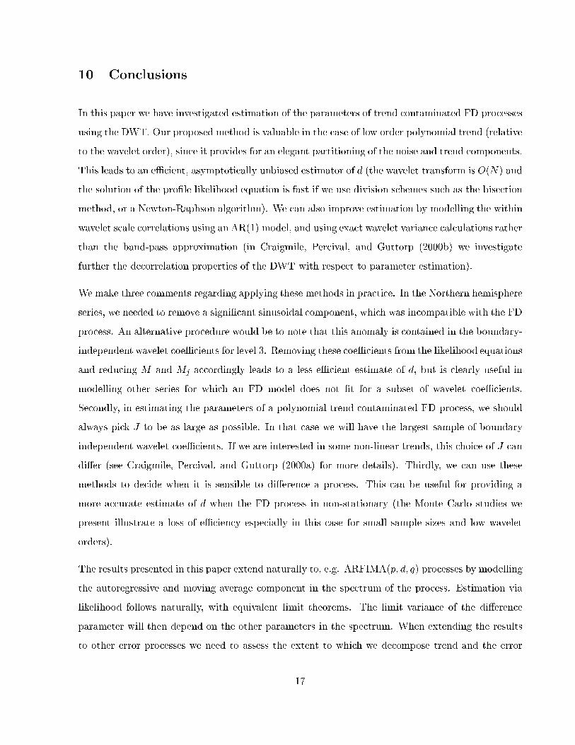
Figure 5: Summary of simulations to estimate the di�erence parameter for N = 256, 512, 1024 and

L = 2, 4, 8 (with 1024 replications for each case). The AR(1) wavelet model was used with exact

wavelet variances. The bootstrap standard deviation (calculated using 2048 bootstrap samples) of

each statistic was bounded by 0.003.

30

Year

Ave

rage

tem

pera

ture

rel

ativ

e to

196

1-19

90

1860 1880 1900 1920 1940 1960 1980 2000

-1.5

-1.0

-0.5

0.0

0.5

1.0

Figure 6: Northern Hemisphere temperature series. The series is the monthly di�erences in degrees

Celsius from 1854 to 1998 relative to the monthly average over the period 1961 to 1990. Source of

this dataset is the Climate Research Unit, University of East Anglia, UK.

Frequency

Spe

ctru

m (

dB)

0 1 2 3 4 5 6

-40

-30

-20

-10

010

Log Frequency

Spe

ctru

m (

dB)

-6 -4 -2 0 2

-40

-30

-20

-10

010

Figure 7: A periodogram of the northern hemisphere temperature set. The log of the spectrum is

shown versus the frequency and log of the frequency. The line on the lower �gure denotes the least

squares �t for f � 12=8.

31

Year

Res

idua

l tem

pera

ture

rela

tive

to

1860 1880 1900 1920 1940 1960 1980 2000-1.5

-1.0

-0.5

0.0

0.5

1.0

Frequency

Spec

trum

(dB)

0 1 2 3 4 5 6

-40-

30-2

0-10

010

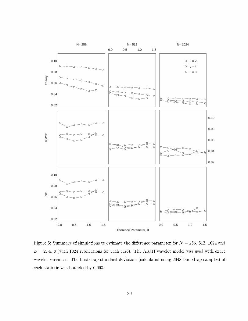
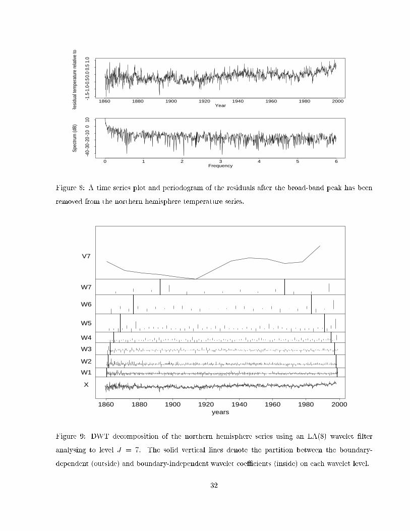
Figure 8: A time series plot and periodogram of the residuals after the broad-band peak has been

removed from the northern hemisphere temperature series.

years1860 1880 1900 1920 1940 1960 1980 2000

X

W1

W2

W3

W4

W5

W6

W7

V7

Figure 9: DWT decomposition of the northern hemisphere series using an LA(8) wavelet �lter

analysing to level J = 7. The solid vertical lines denote the partition between the boundary-

dependent (outside) and boundary-independent wavelet coeÆcients (inside) on each wavelet level.

32

lag0 5 10 15 20 25 30

0.0

0.2

0.4

0.6

0.8

1.0

W1

lag0 5 10 15 20 25

0.0

0.2

0.4

0.6

0.8

1.0

W2

lag0 5 10 15 20-0

.20.0

0.2

0.4

0.6

0.8

1.0

W3

lag0 5 10 15

-0.2

0.0

0.2

0.4

0.6

0.8

1.0

W4

lag0 5 10 15

-0.4

0.0

0.2

0.4

0.6

0.8

1.0

W5

lag0 2 4 6 8 10 12

-0.4

0.0

0.2

0.4

0.6

0.8

1.0

W6

•

••

•

•

•

••

•

•

••

•

•

•

•

•• •

•

•

••

••

••

•

•

••• •

•

•

•

••

•

•

••• •

•

••

• ••

••

•

•

•••

•

••

• •

••

••

••

••

•

••

•••

••••

•

•

• •

••

•

•••••

•• •

•

••

•

••

••

•

••••

•••

•• • •

•

••

••

••••

••

••

•

••• •

•• •• ••

•

••

•

••

••• ••

••

•

••

•••

•

•• •••

••

••

•••••

• • • ••

•••• •

•••• •

•

•

• •• ••

••

•

••••

••

•••

•

•••••

•

••

••

•• •

•••

••

•••

••

•

•

•••

•

• •••

••

•••

•

••• • ••

•

•

• •• ••

•• • • • •

• •••

••

•

••••

•

•••

•

••••••• •

•••••

• ••••

••• • ••••

••

•••

••

••

•

•

•••

••

•

•

• •

••• •

••

• ••

••

••

••

•

••

••

•

••

•

••

••

• • •• •

••

•••

• •

••••••

••

•••

••• ••

•

•

• ••

•

•• •

•••••

•••

••

•

•••

••

•

•

• • ••

•

•••

•••

•

••

••

•

•

•

•• • ••

•••

•

•

•

•• • ••

•

•••

••

•• •••

••

••••

••

•• • •

•

••• •

•

•

•••

• •• •

•••

•

••

• ••

••

••

•

••

••• •••

••

•• • •

•

•

•

•• ••

••••

•

••

••••

• •

•

•• •

••

• •••

•

•

••

••

••

••• ••• ••• •

••• •

••

•

••

• • ••

•

••• •• •••••

•• •• •• •

•• ••• •

•

••••

••

• ••••

•••

•••

•

••••

• • ••• •••

• •••••

••• •

••••

••

••

•

•• • ••

•• ••

••

••••••

•• ••

•• •• • •

••

••••

•

•••••

•• ••• •••

•

• ••

• ••

••

•• ••• •• •

•

•• •

•• •

••••

• •••

•

•••

•• ••

• •• ••• • ••

••

• •

•• ••• • • •• •

•

•

••

••

•

•

•••••

•• ••

•••

•

•• ••

••

••

•

••

•••• • •

• ••• •

•

••• •

•

•

••• •

••

• ••• •••

•••

•

•

•• •

W1

w

-3 -2 -1 0 1 2 3

-0.5

0.0

0.5

••

•

• •

•

••

••

•

••

•

•

••

•

•

•

•

•

•

•

••••

•

•

• •

•••

•

••

•

••

•

•

•

•

••

•

•••

•

••••

•

• •• ••

•

•

••

••

•• •

••

••

•••

•••

••• ••

•• •• ••

•

•

•

•

• ••••

•••• ••• ••

••

•

•••

•

•••••

•

••

•

•• •••

•

•• • •

• ••

••

•••

•••

••••• •

•

•

••

•

•• •

••

••

• •••• •

•

•••

••• •

•

••• •

•

• •

••••••

•

• •• • ••

••

•

••••• • ••

•••

•••

•••

••

•• •

••• ••

•

•••

••

•••

• • ••••

••

•

•

•

••• •

•

•

• •• • •

••

••

•

••

••

••••

•

••

• ••••

•• •• •••

•

•• •••

•

•••

•••

• ••

••

•

•

•• •••

••

•• •

••

•

•

••

••• • ••

•

•••

• ••

•••

•• •••

• • ••• ••

•• ••

•

•

•••

••

•

•••

• •• ••

•••

•• • ••• •

•••

•

••••

•

••

•

• • ••••

••• •

••

•• •

W2

w

-3 -2 -1 0 1 2 3-0

.50.0

0.5

1.0

•• •

•

•

•

•••

•

••

•

••

• •

•

•

•

•

•

•

•

•

•

•

••

•

••

••••

••

••

•

•

•••

•

•

•• •

••

•

•

••

•

•

••

•

•

•

•

• ••

•• •• •

••

• •

•

••

•••

•

••

•

•

•

•

•

•••

• •

••

•

• •

•

•• •

•

•

•

• ••••

••

••

••

• • •

•

•••

•

••• •

••

•

•

•

•

•

•

••

••••

••

• ••

•••

•

• ••

•

••

•

•• •

•

• ••

••••

•

• •

••

•

•

• •

•

••

•

••• ••

••

••

• ••

•

••

•

•

•

W3

w

-3 -2 -1 0 1 2 3

-0.6

-0.2

0.0

0.2

0.4

0.6

•

•

•

•

•

•

•

•

•

•

•••

•

•

•

•

•

•

•

•

•

•

••

••

•

•

•

• •

•

••

•

••

•

•

••

•

•

•

••

•

•

••

•

•

•

•

•••

•

•

••

••

•

••

•••

••

••

•

••

•

•

••

•

••

•

•

• •

•

•

•

•

•

•

••••

W4

w

-2 -1 0 1 2

-0.6

-0.2

0.0

0.2

0.4

0.6

•

•

•

•

••

• •••

•

••

••

•

•

•

•

•

•

•

•

•

• •• ••

••

•

•

•

•

••

•

•

•

•••

•

••

W5

w

-2 -1 0 1 2

-0.5

0.0

0.5

1.0

1.5

•

•

•

•

• •

•

•

• • •

••

•

•

•

•

•

•

•

W6

w

-2 -1 0 1 2

-0.5

0.0

0.5

Figure 10: Normal Q-Q plots and ACFs of the �rst six wavelet scales for the Northern hemisphere

dataset

YearYea

rly A

vera

ge te

mpe

ratu

re r

elat

ive

to 1

961-

1990

1860 1880 1900 1920 1940 1960 1980 2000

-0.6

-0.4

-0.2

0.0

0.2

0.4

0.6

Figure 11: Yearly average of the monthly di�erences in degrees Celsius from 1854 to 1998 relative

to the monthly average over the period 1961 to 1990.

33

White noise wavelet model AR(1) wavelet model

N L J d LogLik Wald Rao LogLik Wald Rao

1024 2 9 0.00 93.85 93.85 93.75 94.04 94.24 94.34

1024 2 9 0.25 88.96 87.99 87.11 89.36 88.57 87.50

1024 2 9 0.50 80.96 78.91 77.93 80.96 81.15 76.95

1024 2 9 0.75 83.59 82.52 82.23 81.15 83.59 76.37

1024 2 9 1.00 82.32 82.23 83.30 80.66 83.69 76.37

1024 2 9 1.25 53.91 54.79 57.23 61.04 66.60 57.81

1024 2 9 1.50 48.93 48.44 50.88 59.38 66.31 55.47

1024 4 8 0.00 94.24 94.92 94.14 93.46 93.75 93.75

1024 4 8 0.25 91.89 92.29 91.21 93.26 93.07 92.68

1024 4 8 0.50 92.48 92.38 90.43 93.07 93.46 91.41

1024 4 8 0.75 90.92 90.43 89.45 93.26 94.92 89.16

1024 4 8 1.00 89.26 88.38 88.18 90.72 95.80 86.72

1024 4 8 1.25 87.01 87.40 88.18 87.21 95.02 76.86

1024 4 8 1.50 73.83 75.00 77.05 68.85 88.67 51.86

1024 8 7 0.00 94.92 95.80 94.24 94.63 94.43 94.63

1024 8 7 0.25 94.04 95.12 92.77 94.63 95.02 94.63

1024 8 7 0.50 92.48 93.85 91.89 93.55 94.43 92.97

1024 8 7 0.75 92.38 92.77 91.11 93.26 95.21 91.31

1024 8 7 1.00 92.09 92.19 90.43 94.14 96.88 90.43

1024 8 7 1.25 88.87 89.75 89.45 92.48 97.95 84.38

1024 8 7 1.50 87.89 88.67 88.77 89.94 98.54 73.73

Table 1: Monte Carlo Simulation of Coverages for Log Likelihood, Wald and Rao 95% Approximate

Con�dence intervals, for various wavelet �lters using the two wavelet estimation models. Each run

had 1024 replications. A band-pass wavelet variance approximation was used.

34