Embed Size (px)
Citation preview
EARTHQUAKE ENGINEERING AND STRUCTURAL DYNAMICSEarthquake Engng Struct. Dyn. 2008; 37:1333–1348Published online 21 April 2008 in Wiley InterScience (www.interscience.wiley.com). DOI: 10.1002/eqe.820
Wavelet-based simulation of spectrum-compatibleaftershock accelerograms
S. Das and V. K. Gupta∗,†
Department of Civil Engineering, Indian Institute of Technology Kanpur, Kanpur 208016, India
SUMMARY
In damage-based seismic design it is desirable to account for the ability of aftershocks to cause furtherdamage to an already damaged structure due to the main shock. Availability of recorded or simulatedaftershock accelerograms is a critical component in the non-linear time-history analyses required for thispurpose, and simulation of realistic accelerograms is therefore going to be the need of the profession fora long time to come. This paper attempts wavelet-based simulation of aftershock accelerograms for twoscenarios. In the first scenario, recorded main shock and aftershock accelerograms are available along withthe pseudo-spectral acceleration (PSA) spectrum of the anticipated main shock motion, and an accelerogramhas been simulated for the anticipated aftershock motion such that it incorporates temporal features ofthe recorded aftershock accelerogram. In the second scenario, a recorded main shock accelerogram isavailable along with the PSA spectrum of the anticipated main shock motion and PSA spectrum andstrong motion duration of the anticipated aftershock motion. Here, the accelerogram for the anticipatedaftershock motion has been simulated assuming that temporal features of the main shock accelerogram arereplicated in the aftershock accelerograms at the same site. The proposed algorithms have been illustratedwith the help of the main shock and aftershock accelerograms recorded for the 1999 Chi–Chi earthquake.It has been shown that the proposed algorithm for the second scenario leads to useful results even whenthe main shock and aftershock accelerograms do not share the same temporal features, as long as strongmotion duration of the anticipated aftershock motion is properly estimated. Copyright q 2008 John Wiley& Sons, Ltd.
Received 8 November 2007; Revised 9 March 2008; Accepted 12 March 2008
KEY WORDS: damage-based design; wavelet transform; aftershocks; synthetic accelerogram
1. INTRODUCTION
The existing earthquake design philosophy does not envisage any role of aftershocks assumingthat those are too weak to cause further damage to an already damaged structure during the main
∗Correspondence to: V. K. Gupta, Department of Civil Engineering, Indian Institute of Technology Kanpur, Kanpur208016, India.
†E-mail: [email protected]
Copyright q 2008 John Wiley & Sons, Ltd.
1334 S. DAS AND V. K. GUPTA
shock. This assumption is not always true, particularly when the main shock causes significantdegradation in the stiffness and/or strength of the structure and the aftershocks are too strong forthe weakened structure. In this situation, even though the structure survives the main shock, itmay collapse during one of the aftershocks. It may be noted that aftershocks occur soon after themain shock and thus it is impractical to repair the damaged structure before the occurrence of theaftershocks. Therefore, as shown by Gupta et al. [1], the yield design levels may have to be raisedto account for aftershocks, particularly when the arrival of energy during the main shock takesplace over a shorter duration.
A proper evaluation of the seismic performance of a structure during a main shock and followingaftershocks would require time-history analyses by using the accelerograms corresponding to themain shock and first few aftershocks. These accelerograms should be compatible with the (design)main shock motion anticipated at the site and in keeping with the present practice of seismic hazardcharacterization, compatibility with the pseudo-spectral acceleration (PSA) spectrum representingsuch an action becomes desirable [2]. Availability of the recorded accelerograms for aftershocksis severely limited at this stage, and even when those are available, their compatibility with thedesign main shock motion is not guaranteed. It is therefore necessary to simulate aftershockaccelerograms that are compatible with the PSA spectrum of the anticipated main shock motion,and no simulation technique seems to have been developed till date to address this long-standingneed of the profession.
An attempt is made in this paper to simulate an accelerogram for an anticipated aftershock motionat a site conditional to the anticipated main shock motion at the same site. It is therefore assumedthat the PSA spectrum and the time–frequency characteristics of the anticipated main shock motionare available. Further, some information is assumed to be available about the anticipated aftershockmotion, either in the form of its time–frequency characteristics or in the form of its PSA spectrumand strong motion duration. Algorithms are thus developed for the following two specific situations,depending on what kind of information is available about the anticipated aftershock motion. Inone, the aftershock accelerogram is simulated to possess the given time–frequency characteristics,specified via a recorded aftershock accelerogram, such that it is consistent with the given PSAspectrum of the anticipated main shock motion. It is assumed that the main shock accelerogram isalso available for the same site as the recorded aftershock accelerogram. In the second situation,the PSA spectrum and strong motion duration of the anticipated aftershock motion are knowninstead of its time–frequency characteristics. In the case of main shocks, these two parameters maybe estimated in terms of the seismological parameters such as magnitude and epicentral distance(e.g. [3–6]), and it is therefore expected that similar models will be available in the time to comefor the aftershocks as well. For the purpose of this paper, these are treated as the input parametersto be provided by the user. The algorithms proposed for both situations are illustrated with thehelp of the main shock and aftershock records of 1999 Chi–Chi earthquake (magnitude ML =7.3,focal depth h=10.33km).
The algorithms proposed in this paper are based on the use of the wavelet transform; hence, abrief review of the wavelet transform as used in the paper is given first for the sake of completeness.
2. REVIEW OF THE WAVELET TRANSFORM
Let f (t) be a function belonging to L2(R)—a space of all finite energy functions. This can bedecomposed into wavelet coefficients and reconstructed back from those by using the wavelet
Copyright q 2008 John Wiley & Sons, Ltd. Earthquake Engng Struct. Dyn. 2008; 37:1333–1348DOI: 10.1002/eqe
WAVELET-BASED SIMULATION 1335
transformation and the inverse wavelet transformation, respectively. The continuous wavelet trans-formation of f (t) is defined with respect to a basis function, �(t), as
W� f (a,b)=〈 f,�a,b〉=∫ ∞
−∞f (t)�̄a,b(t)dt, a,b∈� (1)
with �̄(t) being the complex conjugate of
�a,b(t)=1
|a|1/2�
(t−b
a
)(2)
Here, a is a scale parameter that controls the frequency content of the dilated basis function and bis the shift parameter that localizes the basis function at and around t=b. The function f (t) canbe reconstructed back from the wavelet coefficients, W� f (a,b), as
f (t)= 1
2�C�
∫ ∞
−∞
∫ ∞
−∞1
a2W� f (a,b)�a,b(t)da db (3)
with
C� =∫ ∞
−∞|�̂(�)|2
|�| d�<∞ (4)
In Equation (4), �̂(�) is the Fourier transform of the basis function, �(t), defined as
�̂(�)= 1√2�
∫ ∞
−∞�(t)e−i�t dt (5)
For the present study, the modified L-P wavelet basis as proposed by Basu and Gupta [7] isused. This is represented as
�(t)= 1
�√
�−1
sin(��t)−sin(�t)
t(6)
with � taken as 21/4. For �=2, this basis becomes the same as the L-P basis [8] with poorerfrequency localization and improved time localization. On discretizing and taking a j (=� j ) andbi =(i−1)�b as the discretized values of a and b, respectively [7], f (t) can be reconstructed fromits wavelet coefficients as
f (t)=∑jf j (t) (7)
with
f j (t)= K�b
a j
∑iW� f (a j ,bi )�a j ,bi (t) (8)
and
K = 1
4�C�
(�− 1
�
)(9)
Copyright q 2008 John Wiley & Sons, Ltd. Earthquake Engng Struct. Dyn. 2008; 37:1333–1348DOI: 10.1002/eqe
1336 S. DAS AND V. K. GUPTA
Here, �b is taken as 0.02 s. Further, the decomposed time history f j (t) has energy in the periodband, (2a j/�,2a j ). Thus, if a total number of 32 decomposed time histories are considered withj =−21 to 10, f (t) would span over the period band, 0.044–11.32 s, which is deemed to besufficient for most earthquake accelerograms.
3. SYNTHESIS WITH RECORDED AFTERSHOCK MOTION
For the algorithm developed in this section, a pair of main shock and aftershock accelerogramsrecorded at the same site is assumed to be available such that those have similar temporal featuresas desired in the motions to be simulated. The PSA spectrum for the main shock that will precedethe aftershock motion to be simulated is also assumed to be available. The idea here is that wemodify the recorded aftershock accelerogram, without disturbing the temporal variations of differentfrequency waves, such that the modified motion becomes consistent with the PSA spectrum ofthe anticipated main shock and the recorded main shock motion. There are two wavelet-basedmethods in which such a modification appears possible.
In the first method (Method I), it is assumed that the PSA spectrum of the aftershock motion tobe simulated enjoys the same relationship with the given PSA spectrum of the anticipated mainshock as that by the PSA spectrum of the recorded aftershock motion (with the PSA spectrum ofthe recorded main shock motion). In other words, the period-dependent main-shock-to-aftershockattenuation in PSA spectrum is assumed to remain invariant from event to event. This appearsreasonable if the recorded motions are carefully chosen to accurately reflect the characteristicsexpected in the design motions. Thus, if PSAMain(T ) is the smoothed PSA spectrum of the givenmain shock accelerogram and PSAAft(T ) is the smoothed PSA spectrum of the given aftershockaccelerogram, a non-dimensional factor
�(T )= PSAAft(T )
PSAMain(T )(10)
would describe the period-dependent attenuation from the main shock motion to the aftershockmotion. Thus, the PSA spectrum of the anticipated aftershock can be estimated as
DSAft(T )=�(T )DSMain(T ) (11)
where DSMain(T ) is the (design) PSA spectrum for the anticipated main shock. The recordedaccelerogram of the aftershock may now be modified so as to be compatible with DSAft(T ),following the (wavelet-based) procedure of Mukherjee and Gupta [9]. This procedure preservesthe temporal features of the recorded accelerogram in different frequency bands and works wellfor any combination of the target spectrum and the PSA spectrum of the recorded accelerogram.It may be noted that Method I depends significantly on the correct estimation of DSMain(T ).At very long periods, both PSAMain(T ) and PSAAft(T ) approach zero values and therefore �(T )
may not be reliably estimated. As a result, the modified accelerogram may become unrealistic inthe contribution of very long periods.
For the other method (Method II), it will be desirable to recall the procedure of Mukherjee andGupta [9]. In this procedure, the recorded accelerogram f (t) is decomposed into 32 time histo-ries, f j (t), j =−21,−20, . . . ,10 spanning over the period bands, 0.044–0.053, 0.053–0.063, . . . ,9.52–11.32 s, respectively. Each of these time histories is now uniformly scaled by a suitable
Copyright q 2008 John Wiley & Sons, Ltd. Earthquake Engng Struct. Dyn. 2008; 37:1333–1348DOI: 10.1002/eqe
WAVELET-BASED SIMULATION 1337
scaling factor, � j , so that the accelerogram
f̄ (t)=10∑
j=−21� j f j (t) (12)
becomes compatible with the given PSA spectrum. The factors, � j , j =−21,−20, . . . ,10 areobtained iteratively. In Method II, it is proposed to obtain the scaling factors that would modify therecorded main shock accelerogram so as to be compatible with the PSA spectrum of the anticipatedmain shock motion, and to use those factors in Equation (12) for modifying the recorded aftershockaccelerogram (taken as f (t)).
It may be noted that the scaling factor � j denotes the factor by which the contribution ofthe frequency band corresponding to the scale parameter a j to the recorded motion is scaledup/down for consistency of the modified motion with the target PSA spectrum. This factor is atrue indicator of the change in energy levels between the parent motion and the target motion onlyat higher values of j . Owing to sensitivity of the PSA value (of the target motion) at a periodto the � j ’s corresponding to the bands of longer periods, the � j values for lower j’s undergogreater adjustments (than those demanded by the actual differences in the energy levels) in theprocedure of Mukherjee and Gupta [9] and thus are more fictitious than those for the greater j’s.By assuming identical scaling factors for the main shock and aftershock motions, Method II islikely to lead to aftershock accelerograms with unrealistic PSA values at shorter periods. At longerperiods, however, � j becomes almost the same as the ratio, DSMain(T )/PSAMain(T ), and then,both Methods I and II would lead to the aftershock accelerograms with very similar PSA spectra.
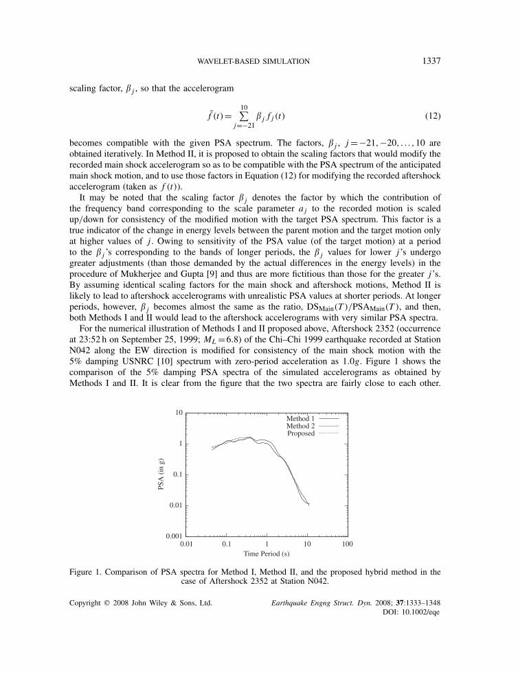
For the numerical illustration of Methods I and II proposed above, Aftershock 2352 (occurrenceat 23:52 h on September 25, 1999; ML =6.8) of the Chi–Chi 1999 earthquake recorded at StationN042 along the EW direction is modified for consistency of the main shock motion with the5% damping USNRC [10] spectrum with zero-period acceleration as 1.0g. Figure 1 shows thecomparison of the 5% damping PSA spectra of the simulated accelerograms as obtained byMethods I and II. It is clear from the figure that the two spectra are fairly close to each other.
0.001
0.01
0.1
1
10
0.01 0.1 1 10 100
PSA
(in
g)
Time Period (s)
Method 1Method 2Proposed
Figure 1. Comparison of PSA spectra for Method I, Method II, and the proposed hybrid method in thecase of Aftershock 2352 at Station N042.
Copyright q 2008 John Wiley & Sons, Ltd. Earthquake Engng Struct. Dyn. 2008; 37:1333–1348DOI: 10.1002/eqe
1338 S. DAS AND V. K. GUPTA
At very long periods, however, the spectrum for Method I appears to be having an unrealistic rateof decay with increase in period, possibly due to the problems with the estimation of �(T ) at verylong periods as discussed above.
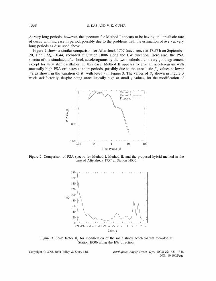
Figure 2 shows a similar comparison for Aftershock 1757 (occurrence at 17:57 h on September20, 1999; ML =6.44) recorded at Station H006 along the EW direction. Here also, the PSAspectra of the simulated aftershock accelerograms by the two methods are in very good agreementexcept for very stiff oscillators. In this case, Method II appears to give an accelerogram withunusually high PSA ordinates at short periods, possibly due to the unrealistic � j values at lowerj’s as shown in the variation of � j with level j in Figure 3. The values of � j shown in Figure 3work satisfactorily, despite being unrealistically high at small j values, for the modification of
0.001
0.01
0.1
1
0.01 0.1 1 10 100
PSA
(in
g)
Time Period (s)
Method 1Method 2Proposed
Figure 2. Comparison of PSA spectra for Method I, Method II, and the proposed hybrid method in thecase of Aftershock 1757 at Station H006.
0
20
40
60
80
100
120
140
160
180
-21 -19 -17 -15 -13 -11 -9 -7 -5 -3 -1 1 3 5 7 9
β j
Level, j
Figure 3. Scale factor � j for modification of the main shock accelerogram recorded atStation H006 along the EW direction.
Copyright q 2008 John Wiley & Sons, Ltd. Earthquake Engng Struct. Dyn. 2008; 37:1333–1348DOI: 10.1002/eqe
WAVELET-BASED SIMULATION 1339
-0.6-0.3
0 0.3 0.6 0.9
0 10 20 30 40 50 60 70 80
accl
(g)
Time (s)
Modified
-0.02-0.01
0 0.01 0.02 0.03
0 10 20 30 40 50 60 70 80ac
cl (
g)
Recorded
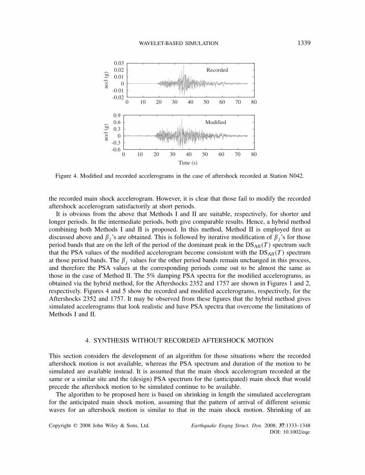
Figure 4. Modified and recorded accelerograms in the case of aftershock recorded at Station N042.
the recorded main shock accelerogram. However, it is clear that those fail to modify the recordedaftershock accelerogram satisfactorily at short periods.
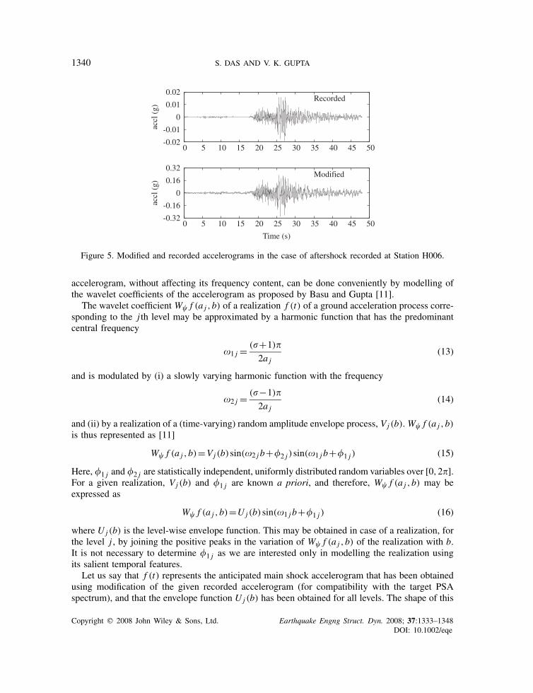
It is obvious from the above that Methods I and II are suitable, respectively, for shorter andlonger periods. In the intermediate periods, both give comparable results. Hence, a hybrid methodcombining both Methods I and II is proposed. In this method, Method II is employed first asdiscussed above and � j ’s are obtained. This is followed by iterative modification of � j ’s for thoseperiod bands that are on the left of the period of the dominant peak in the DSAft(T ) spectrum suchthat the PSA values of the modified accelerogram become consistent with the DSAft(T ) spectrumat those period bands. The � j values for the other period bands remain unchanged in this process,and therefore the PSA values at the corresponding periods come out to be almost the same asthose in the case of Method II. The 5% damping PSA spectra for the modified accelerograms, asobtained via the hybrid method, for the Aftershocks 2352 and 1757 are shown in Figures 1 and 2,respectively. Figures 4 and 5 show the recorded and modified accelerograms, respectively, for theAftershocks 2352 and 1757. It may be observed from these figures that the hybrid method givessimulated accelerograms that look realistic and have PSA spectra that overcome the limitations ofMethods I and II.
4. SYNTHESIS WITHOUT RECORDED AFTERSHOCK MOTION
This section considers the development of an algorithm for those situations where the recordedaftershock motion is not available, whereas the PSA spectrum and duration of the motion to besimulated are available instead. It is assumed that the main shock accelerogram recorded at thesame or a similar site and the (design) PSA spectrum for the (anticipated) main shock that wouldprecede the aftershock motion to be simulated continue to be available.
The algorithm to be proposed here is based on shrinking in length the simulated accelerogramfor the anticipated main shock motion, assuming that the pattern of arrival of different seismicwaves for an aftershock motion is similar to that in the main shock motion. Shrinking of an
Copyright q 2008 John Wiley & Sons, Ltd. Earthquake Engng Struct. Dyn. 2008; 37:1333–1348DOI: 10.1002/eqe
1340 S. DAS AND V. K. GUPTA
-0.32
-0.16
0
0.16
0.32
0 5 10 15 20 25 30 35 40 45 50
accl
(g)
Time (s)
Modified
-0.02
-0.01
0
0.01
0.02
0 5 10 15 20 25 30 35 40 45 50ac
cl (
g)
Recorded
Figure 5. Modified and recorded accelerograms in the case of aftershock recorded at Station H006.
accelerogram, without affecting its frequency content, can be done conveniently by modelling ofthe wavelet coefficients of the accelerogram as proposed by Basu and Gupta [11].
The wavelet coefficient W� f (a j ,b) of a realization f (t) of a ground acceleration process corre-sponding to the j th level may be approximated by a harmonic function that has the predominantcentral frequency
�1 j = (�+1)�
2a j(13)
and is modulated by (i) a slowly varying harmonic function with the frequency
�2 j = (�−1)�
2a j(14)
and (ii) by a realization of a (time-varying) random amplitude envelope process, Vj (b). W� f (a j ,b)is thus represented as [11]
W� f (a j ,b)=Vj (b)sin(�2 j b+�2 j )sin(�1 j b+�1 j ) (15)
Here, �1 j and �2 j are statistically independent, uniformly distributed random variables over [0,2�].For a given realization, Vj (b) and �1 j are known a priori, and therefore, W� f (a j ,b) may beexpressed as
W� f (a j ,b)=Uj (b)sin(�1 j b+�1 j ) (16)
where Uj (b) is the level-wise envelope function. This may be obtained in case of a realization, forthe level j , by joining the positive peaks in the variation of W� f (a j ,b) of the realization with b.It is not necessary to determine �1 j as we are interested only in modelling the realization usingits salient temporal features.
Let us say that f (t) represents the anticipated main shock accelerogram that has been obtainedusing modification of the given recorded accelerogram (for compatibility with the target PSAspectrum), and that the envelope function Uj (b) has been obtained for all levels. The shape of this
Copyright q 2008 John Wiley & Sons, Ltd. Earthquake Engng Struct. Dyn. 2008; 37:1333–1348DOI: 10.1002/eqe
WAVELET-BASED SIMULATION 1341
function for a level j describes the arrival pattern of energy in the waves in the frequency bandcorresponding to the level j . In the absence of any other known linkage between the main shockand aftershock motions, it is assumed here that the identical pattern of energy arrival will holdgood for various aftershocks to be recorded at the same station. This appears reasonable as longas the mechanism of energy release at source during the aftershock can be assumed to be similarto that during the main shock. Considering that the main shocks result from tens or hundreds ofkilometers fault ruptures as against aftershocks that are associated with smaller faults resultingin simpler rupture mechanisms, this assumption may not usually hold good. The impact of thisassumption will therefore be examined later through a numerical study.
Keeping the shape of the envelope function unchanged at all levels, the main shock accelerogrammay be shrunk by a shrink factor k (usually k<1; k>1 implies stretching) and the wavelet coefficientW� f (a j ,b) may be modified to W̄� f (a j ,b) such that
W̄� f (a j ,b)=Uj (b̄)sin(�1 j b+�1 j ) (17)
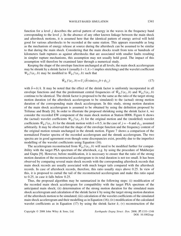
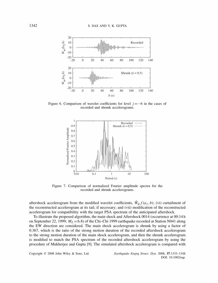
with b̄=b/k. It may be noted that the effect of the shrink factor is uniformly incorporated in allenvelope functions and that the predominant central frequencies of W̄� f (a j ,b) and W� f (a j ,b)continue to be identical. The shrink factor is proposed to be the same as the ratio of the target strongmotion duration (of the aftershock accelerogram to be simulated) to the (actual) strong motionduration of the corresponding main shock accelerogram. In this study, strong motion durationof the main shock accelerogram is assumed to be obtained by using the definition proposed byTrifunac and Brady [6]. In order to illustrate the proposed shrinking using the shrink factor k, weconsider the recorded EW component of the main shock motion at Station H006. Figure 6 showsthe (actual) wavelet coefficients W� f (a j ,b) for the original motion and the (modelled) waveletcoefficients W̄� f (a j ,b) for the shrunk motion with k=0.5, in the case of j =−6 and �1 j assumedarbitrarily. It may be observed that the shape of the envelope function and the frequency content ofthe original motion remain unchanged in the shrunk motion. Figure 7 shows a comparison of thenormalized Fourier spectra of the recorded accelerogram and the shrunk accelerogram. The twospectra are in good agreement even though some discrepancies exist, possibly due to the imperfectmodelling of the wavelet coefficients using Equation (16).
The accelerogram reconstructed from W̄� f (a j ,b) will need to be modified further for compat-ibility with the target PSA spectrum of the aftershock, e.g. by using the procedure of Mukherjeeand Gupta [9]. However, before modification, it is necessary to ensure that the ratio of the strongmotion duration of the reconstructed accelerogram to its total duration is not too small. It has beenobserved by comparing several main shock records with the corresponding aftershock records thatmain shock records are usually associated with much longer tails compared with the aftershockrecords. In case of aftershock records, therefore, this ratio usually stays above 0.25. In view ofthis, it is proposed to curtail the tail of the reconstructed accelerogram and make this ratio equalto 0.25, in case it falls below 0.25.
Thus, the proposed algorithm may be summarized in the following steps: (i) modification ofthe recorded main shock accelerogram for compatibility with the target PSA spectrum of theanticipated main shock; (ii) determination of the strong motion duration for the simulated mainshock accelerogram and calculation of the shrink factor k by using the target strong motion durationof the aftershock motion to be simulated; (iii) calculation of the wavelet coefficients of the simulatedmain shock accelerogram and their modelling as in Equation (16); (iv) modification of the calculatedwavelet coefficients as in Equation (17) by using the shrink factor k; (v) reconstruction of the
Copyright q 2008 John Wiley & Sons, Ltd. Earthquake Engng Struct. Dyn. 2008; 37:1333–1348DOI: 10.1002/eqe
1342 S. DAS AND V. K. GUPTA
-20
-10
0
10
20
-20 0 20 40 60 80 100 120 140
Wψ
f(a j
,b)
b (s)
Shrunk (k = 0.5)
-20
-10
0
10
20
-20 0 20 40 60 80 100 120 140W
ψf(
a j,b
) Recorded
Figure 6. Comparison of wavelet coefficients for level j=−6 in the cases ofrecorded and shrunk accelerograms.
0
0.1
0.2
0.3
0.4
0.5
0.6
0.7
0.8
0.9
1
0.01 0.1 1 10 100
Nor
mal
ized
Fou
rier
Am
plitu
de
Period (s)
RecordedShrunk (k = 0.5)
Figure 7. Comparison of normalized Fourier amplitude spectra for therecorded and shrunk accelerograms.
aftershock accelerogram from the modified wavelet coefficients, W̄� f (a j ,b); (vi) curtailment ofthe reconstructed accelerogram at its tail, if necessary; and (vii) modification of the reconstructedaccelerogram for compatibility with the target PSA spectrum of the anticipated aftershock.
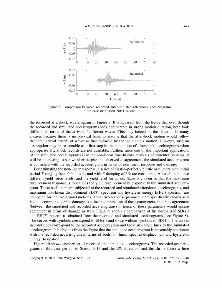
To illustrate the proposed algorithm, the main shock and Aftershock 0014 (occurrence at 00:14 hon September 22, 1999; ML =6.8) of the Chi–Chi 1999 earthquake recorded at Station N041 alongthe EW direction are considered. The main shock accelerogram is shrunk by using a factor of0.367, which is the ratio of the strong motion duration of the recorded aftershock accelerogramto the strong motion duration of the main shock accelerogram, and then the shrunk accelerogramis modified to match the PSA spectrum of the recorded aftershock accelerogram by using theprocedure of Mukherjee and Gupta [9]. The simulated aftershock accelerogram is compared with
Copyright q 2008 John Wiley & Sons, Ltd. Earthquake Engng Struct. Dyn. 2008; 37:1333–1348DOI: 10.1002/eqe
WAVELET-BASED SIMULATION 1343
-0.16
-0.08
0
0.08
0.16
0 10 20 30 40 50 60 70 80
accl
(g)
Time (s)
Recorded
-0.16
-0.08
0
0.08
0.16
0 10 20 30 40 50 60 70 80ac
cl (
g)
Simulated
Figure 8. Comparison between recorded and simulated aftershock accelerogramsin the case of Station N041 record.
the recorded aftershock accelerogram in Figure 8. It is apparent from the figure that even thoughthe recorded and simulated accelerograms look comparable in strong motion duration, both lookdifferent in terms of the arrival of different waves. This may indeed be the situation in manya cases because there is no physical basis to assume that the aftershock motion would followthe same arrival pattern of waves as that followed by the main shock motion. However, such anassumption may be reasonable as a first step in the simulation of aftershock accelerograms whenappropriate aftershock records are not available. Further, since one of the important applicationsof the simulated accelerograms is in the non-linear time-history analyses of structural systems, itwill be interesting to see whether despite the observed disagreement, the simulated accelerogramis consistent with the recorded accelerogram in terms of non-linear response and damage.
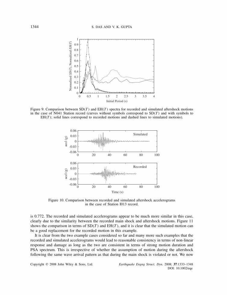
For estimating the non-linear response, a series of elastic–perfectly plastic oscillators with initialperiod T ranging from 0.044 to 4 s and with F-damping of 5% are considered. All oscillators havedifferent yield force levels, and the yield level for an oscillator is chosen so that the maximumdisplacement response is four times the yield displacement in response to the simulated accelero-gram. These oscillators are subjected to the recorded and simulated aftershock accelerograms, andmaximum non-linear displacement SD(T ) spectrum and hysteresis energy EH(T ) spectrum arecompared for the two ground motions. These two response parameters are specifically chosen as itis quite common to define damage as a linear combination of these parameters, and thus, agreement(between the simulated and recorded accelerograms) in terms of these parameters would ensureagreement in terms of damage as well. Figure 9 shows a comparison of the normalized SD(T )
and EH(T ) spectra as obtained from the recorded and simulated accelerograms (see Figure 8).The curves with symbols correspond to EH(T ) and those without symbols to SD(T ). The curvesin solid lines correspond to the recorded accelerogram and those in dashed lines to the simulatedaccelerogram. It is obvious from the figure that the simulated accelerogram is reasonably consistentwith the recorded accelerogram in terms of both non-linear spectral displacement and hysteresisenergy dissipation.
Figure 10 shows another set of recorded and simulated accelerograms. The recorded accelero-grams in this case pertain to Station I013 and the EW direction, and the shrink factor k here
Copyright q 2008 John Wiley & Sons, Ltd. Earthquake Engng Struct. Dyn. 2008; 37:1333–1348DOI: 10.1002/eqe
1344 S. DAS AND V. K. GUPTA
0
0.1
0.2
0.3
0.4
0.5
0.6
0.7
0.8
0.9
1
0 0.5 1 1.5 2 2.5 3 3.5 4
Nor
mal
ized
SD(T
), N
orm
aliz
ed E
H(T
)
Initial Period (s)
Figure 9. Comparison between SD(T ) and EH(T ) spectra for recorded and simulated aftershock motionsin the case of N041 Station record (curves without symbols correspond to SD(T ) and with symbols to
EH(T ); solid lines correspond to recorded motions and dashed lines to simulated motions).
-0.06
-0.03
0
0.03
0.06
0 20 40 60 80 100
accl
(g)
Time (s)
Recorded
-0.06
-0.03
0
0.03
0.06
0 20 40 60 80 100
accl
(g)
Simulated
Figure 10. Comparison between recorded and simulated aftershock accelerogramsin the case of Station I013 record.
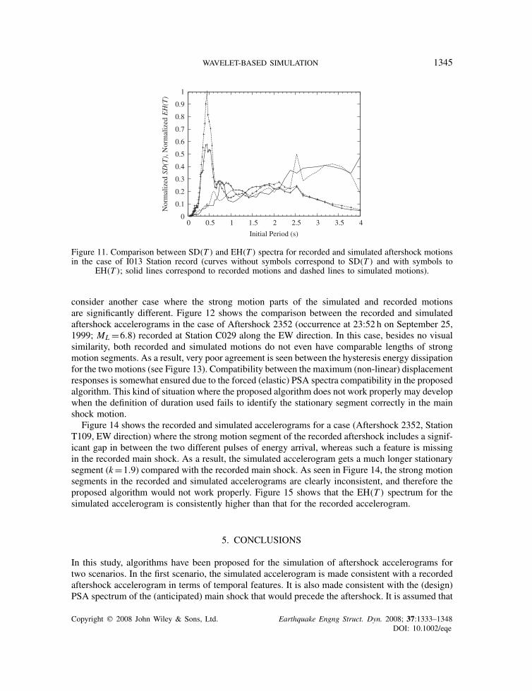
is 0.772. The recorded and simulated accelerograms appear to be much more similar in this case,clearly due to the similarity between the recorded main shock and aftershock motions. Figure 11shows the comparison in terms of SD(T ) and EH(T ), and it is clear that the simulated motion canbe a good replacement for the recorded motion in this example.
It is clear from the two example cases considered so far and many more such examples that therecorded and simulated accelerograms would lead to reasonable consistency in terms of non-linearresponse and damage as long as the two are consistent in terms of strong motion duration andPSA spectrum. This is irrespective of whether the assumption of motion during the aftershockfollowing the same wave arrival pattern as that during the main shock is violated or not. We now
Copyright q 2008 John Wiley & Sons, Ltd. Earthquake Engng Struct. Dyn. 2008; 37:1333–1348DOI: 10.1002/eqe
WAVELET-BASED SIMULATION 1345
0
0.1
0.2
0.3
0.4
0.5
0.6
0.7
0.8
0.9
1
0 0.5 1 1.5 2 2.5 3 3.5 4
Nor
mal
ized
SD(T
), N
orm
aliz
ed E
H(T
)
Initial Period (s)
Figure 11. Comparison between SD(T ) and EH(T ) spectra for recorded and simulated aftershock motionsin the case of I013 Station record (curves without symbols correspond to SD(T ) and with symbols to
EH(T ); solid lines correspond to recorded motions and dashed lines to simulated motions).
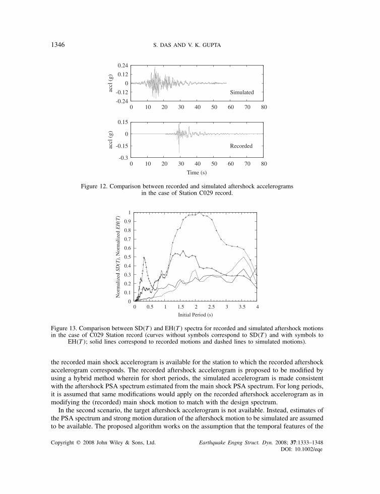
consider another case where the strong motion parts of the simulated and recorded motionsare significantly different. Figure 12 shows the comparison between the recorded and simulatedaftershock accelerograms in the case of Aftershock 2352 (occurrence at 23:52 h on September 25,1999; ML =6.8) recorded at Station C029 along the EW direction. In this case, besides no visualsimilarity, both recorded and simulated motions do not even have comparable lengths of strongmotion segments. As a result, very poor agreement is seen between the hysteresis energy dissipationfor the two motions (see Figure 13). Compatibility between the maximum (non-linear) displacementresponses is somewhat ensured due to the forced (elastic) PSA spectra compatibility in the proposedalgorithm. This kind of situation where the proposed algorithm does not work properly may developwhen the definition of duration used fails to identify the stationary segment correctly in the mainshock motion.
Figure 14 shows the recorded and simulated accelerograms for a case (Aftershock 2352, StationT109, EW direction) where the strong motion segment of the recorded aftershock includes a signif-icant gap in between the two different pulses of energy arrival, whereas such a feature is missingin the recorded main shock. As a result, the simulated accelerogram gets a much longer stationarysegment (k=1.9) compared with the recorded main shock. As seen in Figure 14, the strong motionsegments in the recorded and simulated accelerograms are clearly inconsistent, and therefore theproposed algorithm would not work properly. Figure 15 shows that the EH(T ) spectrum for thesimulated accelerogram is consistently higher than that for the recorded accelerogram.
5. CONCLUSIONS
In this study, algorithms have been proposed for the simulation of aftershock accelerograms fortwo scenarios. In the first scenario, the simulated accelerogram is made consistent with a recordedaftershock accelerogram in terms of temporal features. It is also made consistent with the (design)PSA spectrum of the (anticipated) main shock that would precede the aftershock. It is assumed that
Copyright q 2008 John Wiley & Sons, Ltd. Earthquake Engng Struct. Dyn. 2008; 37:1333–1348DOI: 10.1002/eqe
1346 S. DAS AND V. K. GUPTA
-0.3
-0.15
0
0.15
0 10 20 30 40 50 60 70 80
accl
(g)
Time (s)
Recorded
-0.24
-0.12
0
0.12
0.24
0 10 20 30 40 50 60 70 80ac
cl (
g)
Simulated
Figure 12. Comparison between recorded and simulated aftershock accelerogramsin the case of Station C029 record.
0
0.1
0.2
0.3
0.4
0.5
0.6
0.7
0.8
0.9
1
0 0.5 1 1.5 2 2.5 3 3.5 4
Nor
mal
ized
SD(T
), N
orm
aliz
ed E
H(T
)
Initial Period (s)
Figure 13. Comparison between SD(T ) and EH(T ) spectra for recorded and simulated aftershock motionsin the case of C029 Station record (curves without symbols correspond to SD(T ) and with symbols to
EH(T ); solid lines correspond to recorded motions and dashed lines to simulated motions).
the recorded main shock accelerogram is available for the station to which the recorded aftershockaccelerogram corresponds. The recorded aftershock accelerogram is proposed to be modified byusing a hybrid method wherein for short periods, the simulated accelerogram is made consistentwith the aftershock PSA spectrum estimated from the main shock PSA spectrum. For long periods,it is assumed that same modifications would apply on the recorded aftershock accelerogram as inmodifying the (recorded) main shock motion to match with the design spectrum.
In the second scenario, the target aftershock accelerogram is not available. Instead, estimates ofthe PSA spectrum and strong motion duration of the aftershock motion to be simulated are assumedto be available. The proposed algorithm works on the assumption that the temporal features of the
Copyright q 2008 John Wiley & Sons, Ltd. Earthquake Engng Struct. Dyn. 2008; 37:1333–1348DOI: 10.1002/eqe
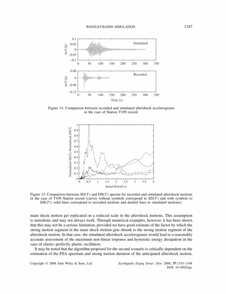
WAVELET-BASED SIMULATION 1347
-0.12
-0.06
0
0.06
0 50 100 150 200 250 300 350
accl
(g)
Time (s)
Recorded
-0.1
-0.05
0
0.05
0.1
0 50 100 150 200 250 300 350ac
cl (
g)
Simulated
Figure 14. Comparison between recorded and simulated aftershock accelerogramsin the case of Station T109 record.
0
0.1
0.2
0.3
0.4
0.5
0.6
0.7
0.8
0.9
1
0 0.5 1 1.5 2 2.5 3 3.5 4
Nor
mal
ized
SD(T
), N
orm
aliz
ed E
H(T
)
Initial Period (s)
Figure 15. Comparison between SD(T ) and EH(T ) spectra for recorded and simulated aftershock motionsin the case of T109 Station record (curves without symbols correspond to SD(T ) and with symbols to
EH(T ); solid lines correspond to recorded motions and dashed lines to simulated motions).
main shock motion get replicated on a reduced scale in the aftershock motions. This assumptionis unrealistic and may not always work. Through numerical examples, however, it has been shownthat this may not be a serious limitation, provided we have good estimate of the factor by which thestrong motion segment in the main shock motion gets shrunk to the strong motion segment of theaftershock motion. In that case, the simulated aftershock accelerograms would lead to a reasonablyaccurate assessment of the maximum non-linear response and hysteretic energy dissipation in thecase of elastic–perfectly plastic oscillators.
It may be noted that the algorithm proposed for the second scenario is critically dependent on theestimation of the PSA spectrum and strong motion duration of the anticipated aftershock motion.
Copyright q 2008 John Wiley & Sons, Ltd. Earthquake Engng Struct. Dyn. 2008; 37:1333–1348DOI: 10.1002/eqe

1348 S. DAS AND V. K. GUPTA
Statistical analyses therefore need to be carried out to establish correlations of the PSA spectraand strong motion durations of aftershocks with the PSA spectra and strong motion durations ofmain shocks. This aspect will be dealt with in another paper by the authors.
ACKNOWLEDGEMENTS
The authors are grateful to Dr Chien-Fu Wu of Seismology Center of Central Weather Bureau, Taipei,Taiwan for making the recorded data for the Chi–Chi earthquake and its aftershocks available for thisstudy.
REFERENCES
1. Gupta VK, Nielsen SRK, Kirkegaard PH. A preliminary prediction of seismic damage-based degradation in RCstructures. Earthquake Engineering and Structural Dynamics 2001; 30:981–993.
2. Hancock J, Watson-Lamprey J, Abrahamson NA, Bommer JJ, Markatis A, McCoy E, Mendis R. An improvedmethod of matching response spectra of recorded earthquake ground motion using wavelets. Journal of EarthquakeEngineering 2006; 10(1):67–89.
3. Johnson RA. An earthquake spectrum prediction technique. Bulletin of the Seismological Society of America1973; 63(4):1255–1274.
4. McGuire RK. Seismic design spectra and mapping procedures using hazard analysis based directly on oscillatorresponse. Earthquake Engineering and Structural Dynamics 1977; 5:211–234.
5. Kamiyama M, Yanagisawa E. A statistical model for estimating response spectra of strong earthquake groundmotions with emphasis on local soil conditions. Soils and Foundations 1986; 26(2):16–32.
6. Trifunac MD, Brady AG. A study on the duration of strong earthquake ground motion. Bulletin of the SeismologicalSociety of America 1975; 65:581–626.
7. Basu B, Gupta VK. Seismic response of SDOF systems by wavelet modelling of nonstationary processes. Journalof Engineering Mechanics (ASCE) 1998; 124(10):1142–1150.
8. Daubechies I. Ten Lectures on Wavelets. Society for Industrial and Applied Mathematics: Philadelphia, PA,U.S.A., 1992.
9. Mukherjee S, Gupta VK. Wavelet-based generation of spectrum-compatible time-histories. Soil Dynamics andEarthquake Engineering 2002; 22:799–804.
10. USNRC. Design Response Spectra for Seismic Design of Nuclear Power Plants, Regulatory Guide 1.60. UnitedStates Nuclear Regulatory Commission, 1973.
11. Basu B, Gupta VK. Stochastic seismic response of single-degree-of-freedom systems through wavelets. EngineeringStructures 2000; 22:1714–1722.
Copyright q 2008 John Wiley & Sons, Ltd. Earthquake Engng Struct. Dyn. 2008; 37:1333–1348DOI: 10.1002/eqe