Embed Size (px)
DESCRIPTION
image compression
Citation preview

Wavelets (Chapter 7)
CS474/674 – Prof. Bebis

STFT (revisited)
• Time/Frequency localization depends on window size. • Once you choose a particular window size, it will be the same
for all frequencies. • Many signals require a more flexible approach - vary the
window size to determine more accurately either time or frequency.

The Wavelet Transform
• Overcomes the preset resolution problem of the STFT by using a variable length window:
!– Use narrower windows at high frequencies for better time
resolution. !
– Use wider windows at low frequencies for better frequency resolution.

The Wavelet Transform (cont’d)
Wide windows do not provide good localization at high frequencies.
The Wavelet Transform (cont’d)
Use narrower windows at high frequencies.
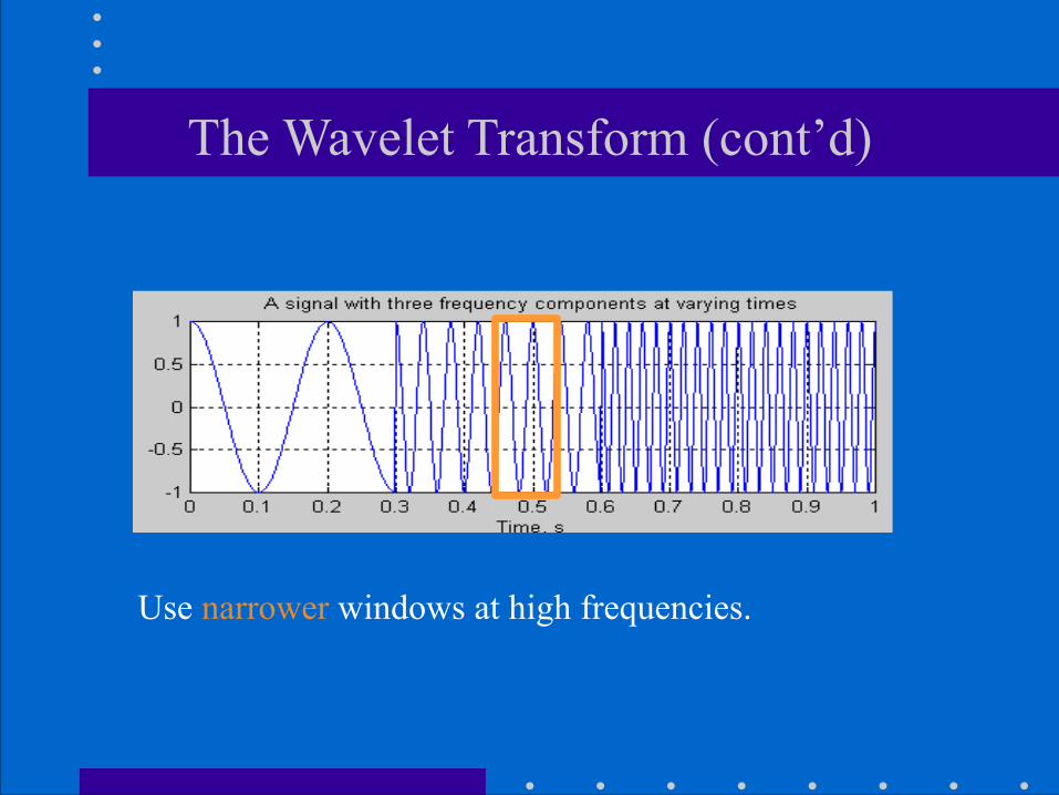
The Wavelet Transform (cont’d)
Narrow windows do not provide good localization at low frequencies.

The Wavelet Transform (cont’d)
Use wider windows at low frequencies.

What are Wavelets?• Wavelets are functions that “wave” above and below the
x-axis, have (1) varying frequency, (2) limited duration, and (3) an average value of zero. !
• This is in contrast to sinusoids, used by FT, which have infinite energy.
Sinusoid Wavelet

What are Wavelets? (cont’d)• Like sines and cosines in FT, wavelets are used as basis
functions ψk(t) in representing other functions f(t): !!!!
• Span of ψk(t): vector space S containing all functions f(t) that can be represented by ψk(t).
( ) ( )k kk
f t a tψ=∑

What are Wavelets? (cont’d)!
• There are many different wavelets:
MorletHaar Daubechies

(dyadic/octave grid)
What are Wavelets? (cont’d)
( ) jk tψ=
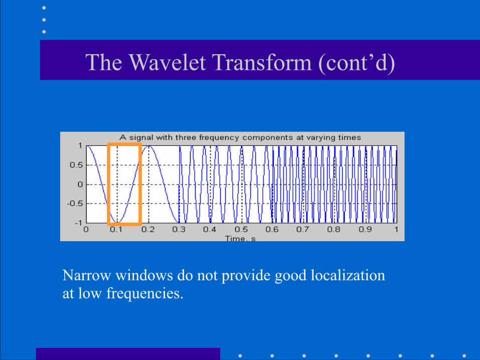
What are Wavelets? (cont’d)
time localization
scale/frequency localization
( )/2( ) 2 2 j jjk t t kψ ψ= −
j

Continuous Wavelet Transform (CWT)
( )1( , )t
tC s f t dtssτ
τ ψ ∗ −% &= ' () *∫
Continuous Wavelet Transform of signal f(t)
translation parameter, measure of time
scale parameter (measure of frequency)
Mother wavelet (window)
normalization constant
Forward CWT:
Scale = 1/j = 1/Frequency

CWT: Main Steps
1. Take a wavelet and compare it to a section at the start of the original signal. !
2. Calculate a number, C, that represents how closely correlated the wavelet is with this section of the signal. The higher C is, the more the similarity.

CWT: Main Steps (cont’d)
3. Shift the wavelet to the right and repeat steps 1 and 2 until you've covered the whole signal.

CWT: Main Steps (cont’d)
4. Scale the wavelet and repeat steps 1 through 3. !!!!!!!5. Repeat steps 1 through 4 for all scales.

Coefficients of CTW Transform
( )1( , )t
tC s f t dtssτ
τ ψ ∗ −% &= ' () *∫
• Wavelet analysis produces a time-scale view of the input signal or image.

Continuous Wavelet Transform (cont’d)
• Inverse CWT:
1( ) ( , ) ( )s
tf t C s d dsss τ
ττ ψ τ
−= ∫ ∫
double integral!

FT vs WT
weighted by F(u)
weighted by C(τ,s)

Properties of Wavelets
• Simultaneous localization in time and scale - The location of the wavelet allows to explicitly represent
the location of events in time. - The shape of the wavelet allows to represent different
detail or resolution.

Properties of Wavelets (cont’d)
• Sparsity: for functions typically found in practice, many of the coefficients in a wavelet representation are either zero or very small. !!!
• Linear-time complexity: many wavelet transformations can be accomplished in O(N) time.
1( ) ( , ) ( )s
tf t C s d dsss τ
ττ ψ τ
−= ∫ ∫

Properties of Wavelets (cont’d)
• Adaptability: wavelets can be adapted to represent a wide variety of functions (e.g., functions with discontinuities, functions defined on bounded domains etc.). – Well suited to problems involving images, open or closed
curves, and surfaces of just about any variety. – Can represent functions with discontinuities or corners more
efficiently (i.e., some have sharp corners themselves).

Discrete Wavelet Transform (DWT)
( ) ( )jk jkk j
f t a tψ=∑∑
( )/2( ) 2 2 j jjk t t kψ ψ= −
(inverse DWT)
(forward DWT)
where
*( ) ( )jkjkt
a f t tψ=∑

DFT vs DWT
• FT expansion: !!!!
• WT expansion
or
one parameter basis
( ) ( )l ll
f t a tψ=∑
( ) ( )jk jkk j
f t a tψ=∑∑
two parameter basis

Multiresolution Representation using
( ) ( )jk jkk j
f t a tψ=∑ ∑
( )f t
( )jk tψ
j
fine details
coarse details
wider, large translations

Multiresolution Representation using
( ) ( )jk jkk j
f t a tψ=∑ ∑
( )f t
( )jk tψ
j
fine details
coarse details

Multiresolution Representation using
( ) ( )jk jkk j
f t a tψ=∑ ∑
( )f t
( )jk tψ
j
fine details
coarse details
narrower, small translations

Multiresolution Representation using
high resolution (more details)
low resolution (less details)
…
( ) ( )jk jkk j
f t a tψ=∑ ∑
( )f t
1̂( )f t
2̂ ( )f t
ˆ ( )sf t
( )jk tψ
j

Prediction Residual Pyramid (revisited)
• In the absence of quantization errors, the approximation pyramid can be reconstructed from the prediction residual pyramid. !• Prediction residual pyramid can be represented more efficiently.
(with sub-sampling)

Efficient Representation Using “Details”
details D2
L0
details D3
details D1
(no sub-sampling)

Efficient Representation Using Details (cont’d)
representation: L0 D1 D2 D3
A wavelet representation of a function consists of (1)a coarse overall approximation (2)detail coefficients that influence the function at various scales.
(decomposition or analysis)in general: L0 D1 D2 D3…DJ

Reconstruction (synthesis)H3=L2+D3
details D2
L0
details D3
H2=L1+D2
H1=L0+D1
details D1
(no sub-sampling)
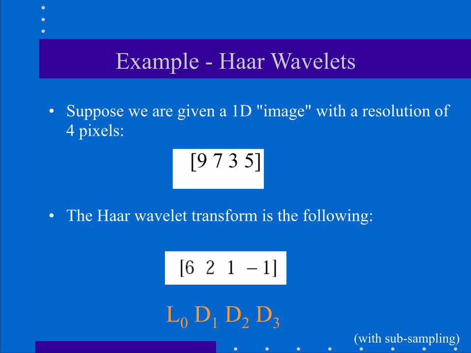
Example - Haar Wavelets
• Suppose we are given a 1D "image" with a resolution of 4 pixels:
[9 7 3 5] !
• The Haar wavelet transform is the following:
L0 D1 D2 D3(with sub-sampling)

Example - Haar Wavelets (cont’d)
• Start by averaging the pixels together (pairwise) to get a new lower resolution image: !
!• To recover the original four pixels from the two
averaged pixels, store some detail coefficients.

Example - Haar Wavelets (cont’d)
• Repeating this process on the averages gives the full decomposition:

Example - Haar Wavelets (cont’d)
• The Harr decomposition of the original four-pixel image is:
!!• We can reconstruct the original image to a resolution
by adding or subtracting the detail coefficients from the lower-resolution versions.
2 1 -1

Example - Haar Wavelets (cont’d)
Note small magnitude detail coefficients!
Dj
Dj-1
D1L0
How to compute Di ?

Multiresolution Conditions• If a set of functions can be represented by a weighted
sum of ψ(2jt - k), then a larger set, including the original, can be represented by a weighted sum of ψ(2j
+1t - k):
time localization
scale/frequency localization
low resolution
high resolution
j

Multiresolution Conditions (cont’d)• If a set of functions can be represented by a weighted
sum of ψ(2jt - k), then a larger set, including the original, can be represented by a weighted sum of ψ(2j
+1t - k):
Vj: span of ψ(2jt - k): ( ) ( )j k jkk
f t a tψ=∑
Vj+1: span of ψ(2j+1t - k): 1 ( 1)( ) ( )j k j k
kf t b tψ+ +=∑
1j jV V +⊆

Nested Spaces Vj
ψ(t - k)
ψ(2t - k)
ψ(2jt - k)
…
V0
V1
Vj
Vj : space spanned by ψ(2jt - k)
Multiresolution conditions à nested spanned spaces:
( ) ( )jk jkk j
f t a tψ=∑ ∑f(t) ϵ Vj
Basis functions:
i.e., if f(t) ϵ V j then f(t) ϵ V j+1
1j jV V +⊂

How to compute Di ?
( ) ( )jk jkk j
f t a tψ=∑ ∑f(t) ϵ Vj
IDEA: define a set of basis functions that span the differences between Vj

Orthogonal Complement Wj
• Let Wj be the orthogonal complement of Vj in Vj+1
Vj+1 = Vj + Wj
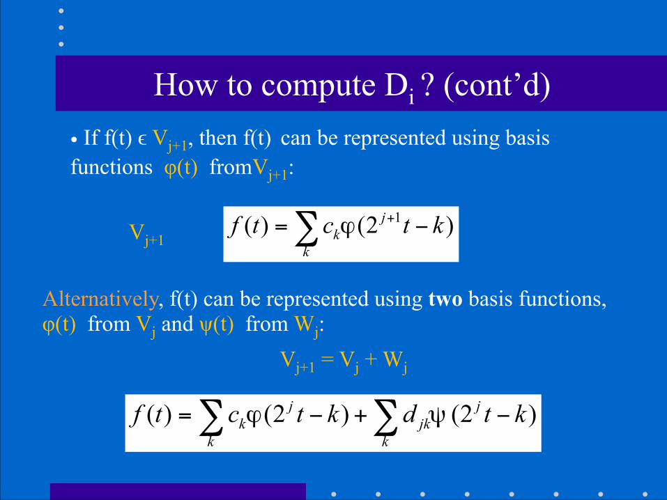
How to compute Di ? (cont’d)• If f(t) ϵ Vj+1, then f(t) can be represented using basis functions φ(t) fromVj+1: !!!!
1( ) (2 )jk
kf t c t kϕ += −∑
( ) (2 ) (2 )j jk jk
k kf t c t k d t kϕ ψ= − + −∑ ∑
Vj+1 = Vj + Wj
Alternatively, f(t) can be represented using two basis functions, φ(t) from Vj and ψ(t) from Wj:
Vj+1

Think of Wj as a means to represent the parts of a function in Vj+1 that cannot be represented in Vj
1( ) (2 )jk
kf t c t kϕ += −∑
( ) (2 ) (2 )j jk jk
k kf t c t k d t kϕ ψ= − + −∑ ∑
Vj, Wj
How to compute Di ? (cont’d)
differences between Vj and Vj+1

How to compute Di ? (cont’d)• à using recursion on Vj:
( ) ( ) (2 )jk jk
k k jf t c t k d t kϕ ψ= − + −∑ ∑∑
V0 W0, W1, W2, … basis functions basis functions
Vj+1 = Vj-1+Wj-1+Wj = …= V0 + W0 + W1 + W2 + … + Wj
if f(t) ϵ Vj+1 , then:
Vj+1 = Vj + Wj

Summary: wavelet expansion (Section 7.2)
• Efficient wavelet decompositions involves a pair of waveforms (mother wavelets): !
!!
• The two shapes are translated and scaled to produce wavelets (wavelet basis) at different locations and on different scales.
φ(t) ψ(t)
φ(t-k) ψ(2jt-k)
encode low resolution info
encode details or high resolution info

Summary: wavelet expansion (cont’d)
• f(t) is written as a linear combination of φ(t-k) and ψ(2jt-k) :
( ) ( ) (2 )jk jk
k k jf t c t k d t kϕ ψ= − + −∑ ∑∑
scaling function wavelet function
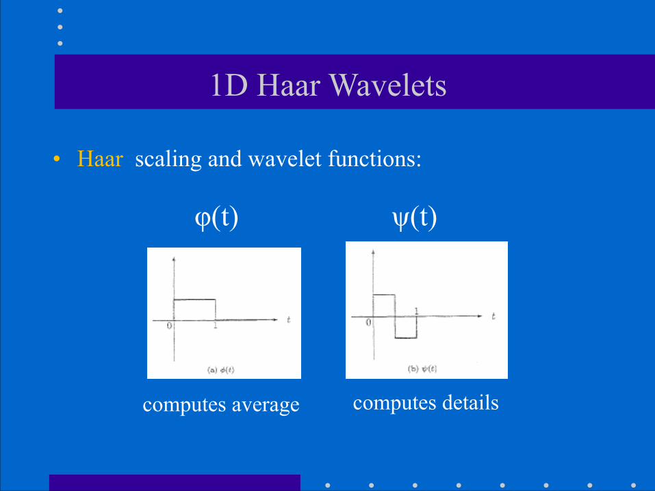
1D Haar Wavelets
• Haar scaling and wavelet functions:
computes average computes details
φ(t) ψ(t)

1D Haar Wavelets (cont’d)
• Think of a one-pixel image as a function that is constant over [0,1) !!
• We will denote by V0 the space of all such functions.
Example:0 1

1D Haar Wavelets
• Think of a two-pixel image as a function having two constant pieces over the intervals [0, 1/2) and [1/2,1) !!!
• We will denote by V1 the space of all such functions. !
• Note that
Examples: 0 ½ 1
0 1V V⊂
= +
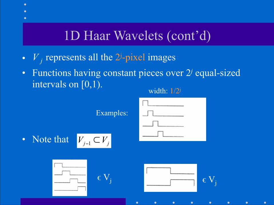
1D Haar Wavelets (cont’d)• V j represents all the 2j-pixel images • Functions having constant pieces over 2j equal-sized
intervals on [0,1). !!!
• Note that
Examples:
width: 1/2j
ϵ Vj ϵ Vj
1j jV V− ⊂

1D Haar Wavelets (cont’d)
V0, V1, ..., V j are nested
i.e.,
VJ … !V2 V1
coarse details
fine details
1j jV V +⊂

1D Haar Wavelets (cont’d)
• Mother scaling function: !!
!• Let’s define a basis for V j :
0 1
note alternative notation: ( ) ( )ji jix xϕ ϕ≡
1

1D Haar Wavelets (cont’d)

1D Haar Wavelets (cont’d)
• Suppose Wj is the orthogonal complement of Vj in Vj+1

1D Haar Wavelets (cont’d)
• Mother wavelet function: !!!!
• Note that φ(x) . ψ(x) = 0 (i.e., orthogonal)
1-1
0 1/2 1
0 1 . = 0 1
-1 0 1/2 1
1

1D Haar Wavelets (cont’d)
• Mother wavelet function: !!!!
• Let’s define a basis ψ ji for Wj :
1-1
0 1
( ) ( )ji jix xψ ψ≡note alternative notation:
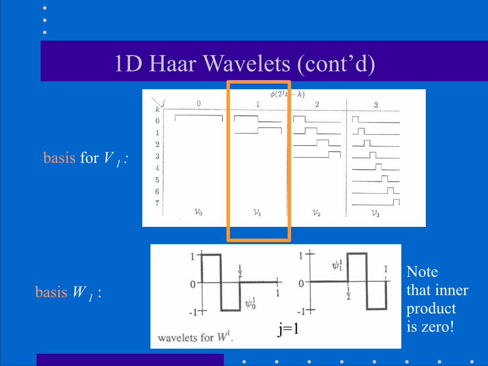
1D Haar Wavelets (cont’d)
j=1
basis W 1 :
basis for V 1 :
Note that inner product is zero!

1D Haar Wavelets (cont’d)
Basis functions ψ ji of W j Basis functions φ ji of V j
form a basis in V j+1
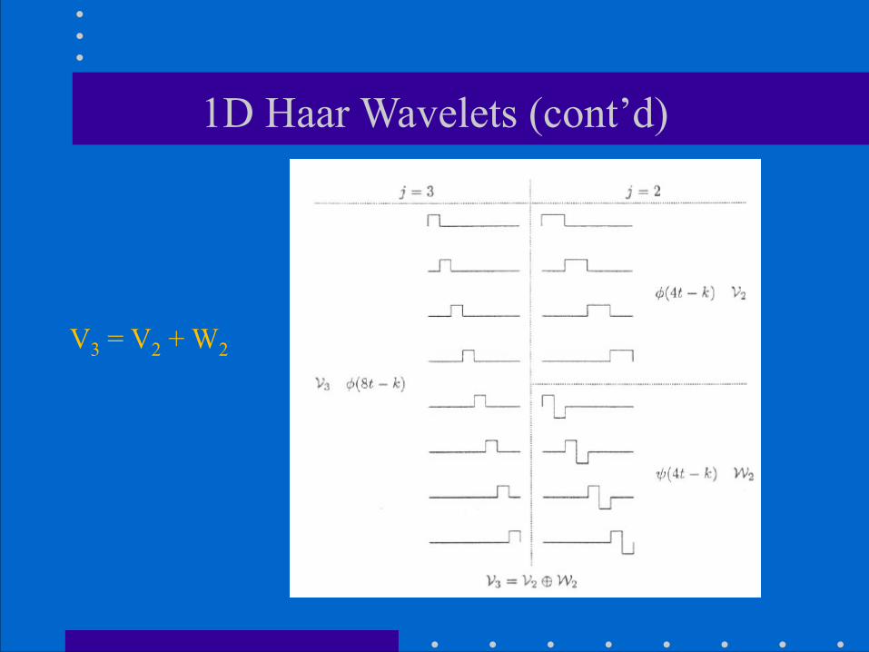
1D Haar Wavelets (cont’d)
V3 = V2 + W2

1D Haar Wavelets (cont’d)
V2 = V1 + W1

1D Haar Wavelets (cont’d)
V1 = V0 + W0
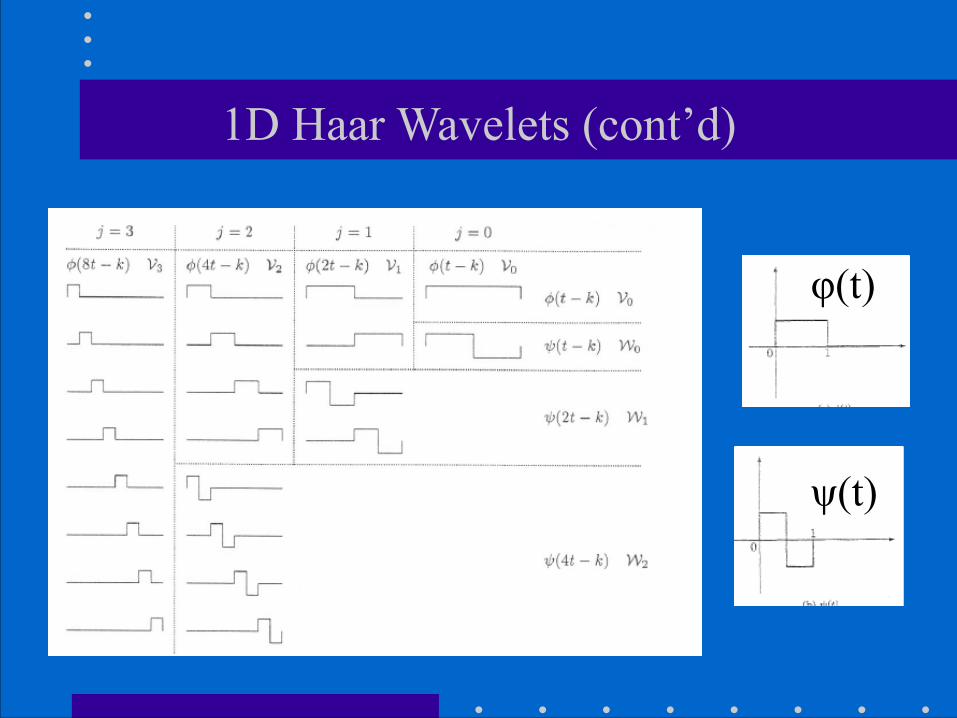
1D Haar Wavelets (cont’d)
ψ(t)
φ(t)

Example - Haar basis (revisited)

Decomposition of f(x)
V2
φ0,2(x)
φ1,2(x)
φ2,2(x)
φ3,2(x)
f(x)=

Decomposition of f(x) (cont’d)
V1and W1
V2=V1+W1
φ0,1(x)
φ1,1(x)
ψ0,1(x)
ψ1,1(x)

Example - Haar basis (revisited)
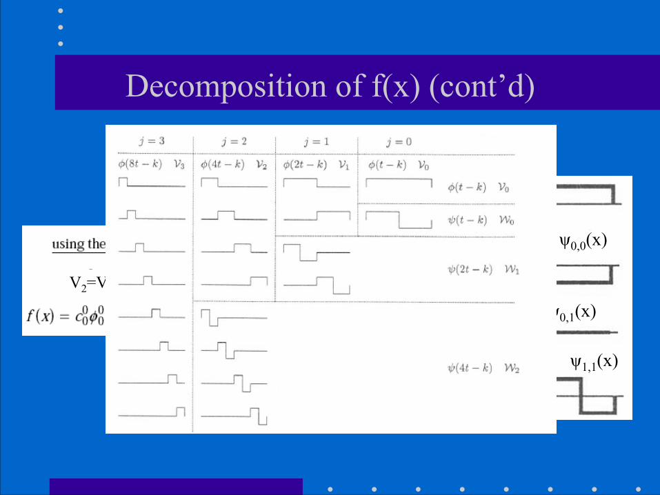
Decomposition of f(x) (cont’d)
V2=V1+W1=V0+W0+W1
V0 ,W0 and W1
φ0,0(x)
ψ0,0(x)
ψ0,1(x)
ψ1,1(x)

Example - Haar basis (revisited)

Example

Example (cont’d)

Filter banks (analysis)
• The lower resolution coefficients can be calculated from the higher resolution coefficients by a tree-structured algorithm (filter bank).
a0k (j=0)
a1k (j=1)
ψ(t - k)
0 0 0ˆ ( ) ( )k k
k jf t a tψ=∑∑
1 1 1ˆ ( ) ( )k k
k jf t a tψ=∑∑
ψ(2t - k) Example:

Filter banks (analysis) (cont’d)• The lower resolution coefficients can be calculated
from the higher resolution coefficients by a tree-structured algorithm (filter bank).
h0(-n) is a lowpass filter and h1(-n) is a highpass filter
Subband encoding!

Example - Haar basis (revisited)
[9 7 3 5]low-pass, down-sampling
high-pass, down-sampling
(9+7)/2 (3+5)/2 (9-7)/2 (3-5)/2 V1 basis functions

Filter banks (analysis) (cont’d)

Example - Haar basis (revisited)
[9 7 3 5]
high-pass, down-sampling
low-pass, down-sampling
(8+4)/2 (8-4)/2
V1 basis functions

Convention for illustrating 1D Haar wavelet decomposition
x x x x x x … x x
detailaverage
…
re-arrange:
re-arrange:
V1 basis functions
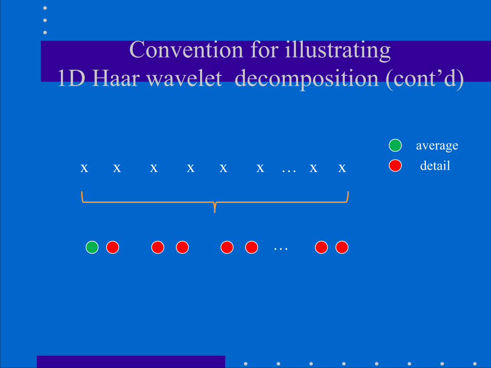
Convention for illustrating 1D Haar wavelet decomposition (cont’d)
x x x x x x … x x detailaverage
…

Orthogonality and normalization
• The Haar basis forms an orthogonal basis • It can become orthonormal through the following
normalization:
since ( ) 2 , ( ) 2j jji jix xϕ ψ− −= =
/2
/2
( ) 1/ 2 (2 ) 2 (2 )
( ) 1/ 2 (2 ) 2 (2 )
j j j j ji
j j j j ji
x x i x i
x x i x i
φ φ φ
ψ ψ ψ
−
−
= − = −
= − = −

Examples of lowpass/highpass analysis filters
Daubechies
Haarh0
h1
h0
h1

Filter banks (synthesis)
• The higher resolution coefficients can be calculated from the lower resolution coefficients using a similar structure.

Filter banks (synthesis) (cont’d)

Examples of lowpass/highpass synthesis filters
Daubechies
Haar (same as for analysis):
+
g0
g1
g0
g1

2D Haar Wavelet Transform
• The 2D Haar wavelet decomposition can be computed using 1D Haar wavelet decompositions (i.e., 2D Haar wavelet basis is separable).
• Two decompositions – Standard decomposition – Non-standard decomposition
• Each decomposition corresponds to a different set of 2D basis functions.

Standard Haar wavelet decomposition
• Steps ! (1) Compute 1D Haar wavelet decomposition of each row of
the original pixel values. !
(2) Compute 1D Haar wavelet decomposition of each column of the row-transformed pixels.

Standard Haar wavelet decomposition (cont’d)
x x x … x x x x … x !… … . x x x ... x
(1) row-wise Haar decomposition:
…
detailaverage
…
… … .
…
…
… … .
re-arrange terms

Standard Haar wavelet decomposition (cont’d)
(1) row-wise Haar decomposition:
…
detailaverage
…
…… … .
…
… … . …
row-transformed resultfrom previous slide:

Standard Haar wavelet decomposition (cont’d)
(2) column-wise Haar decomposition:
…
detailaverage
…
…… … .
……
…… … .
…
row-transformed result column-transformed result

Example
……
…… … .
row-transformed result
…
… … .
re-arrange terms

Example (cont’d)
……
…… … .
column-transformed result

2D Haar basis for standard decompositionTo construct the standard 2D Haar wavelet basis, consider all possible outer products of 1D basis functions.
φ0,0(x)
ψ0,0(x)
ψ0,1(x)
ψ1,1(x)
V2=V0+W0+W1
Example:

2D Haar basis for standard decompositionTo construct the standard 2D Haar wavelet basis, consider all possible outer products of 1D basis functions.
φ00(x), φ00(x) ψ00(x), φ00(x) ψ01(x), φ00(x)
( ) ( )ji jix xϕ ϕ≡ ( ) ( )j
i jix xψ ψ≡

2D Haar basis of standard decomposition
( ) ( )ji jix xϕ ϕ≡
( ) ( )ji jix xψ ψ≡
V2
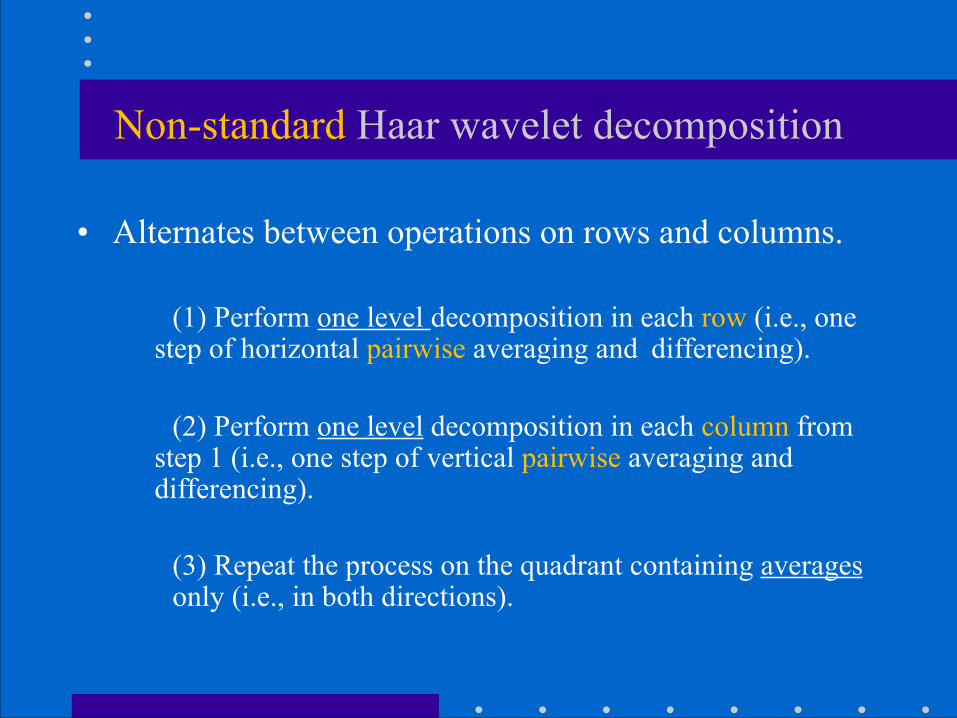
Non-standard Haar wavelet decomposition
• Alternates between operations on rows and columns. ! (1) Perform one level decomposition in each row (i.e., one
step of horizontal pairwise averaging and differencing). ! (2) Perform one level decomposition in each column from
step 1 (i.e., one step of vertical pairwise averaging and differencing).
! (3) Repeat the process on the quadrant containing averages
only (i.e., in both directions).

Non-standard Haar wavelet decomposition (cont’d)
x x x … x x x x … x !… … . x x x . . . x
one level, horizontal Haar decomposition:
……
… … .
…
……
… … .
one level, vertical Haar decomposition:
…
Note: averaging/differencing of detail coefficients shown

Non-standard Haar wavelet decomposition (cont’d)
one level, horizontal Haar decomposition on “green” quadrant
one level, vertical Haar decomposition on “green” quadrant
……
… … .
……
re-arrange terms
……
…… … .
…
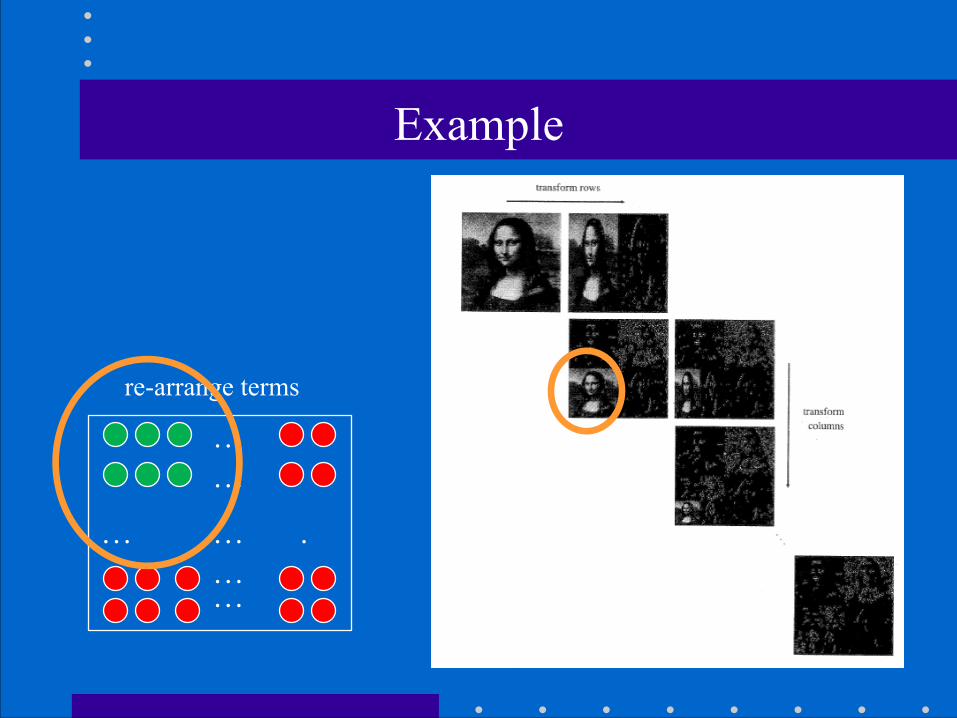
Example
……
… … .
……
re-arrange terms

Example (cont’d)
……
…… … .
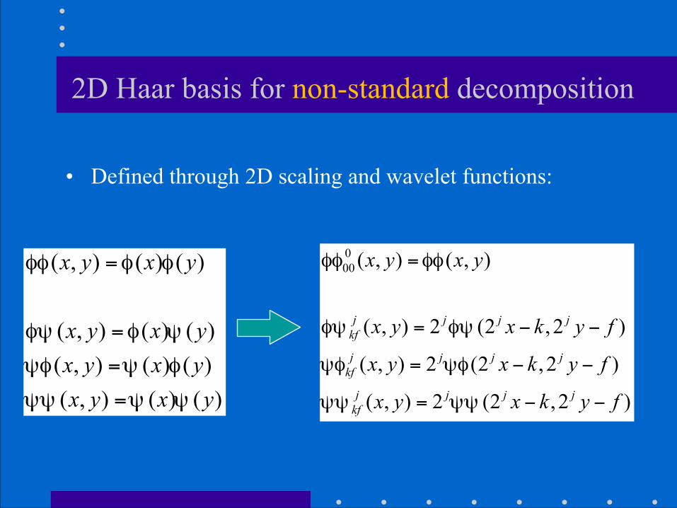
2D Haar basis for non-standard decomposition
!• Defined through 2D scaling and wavelet functions:
( , ) ( ) ( )
( , ) ( ) ( )( , ) ( ) ( )( , ) ( ) ( )
x y x y
x y x yx y x yx y x y
φφ φ φ
φψ φ ψ
ψφ ψ φ
ψψ ψ ψ
=
=
=
=
000 ( , ) ( , )
( , ) 2 (2 ,2 )
( , ) 2 (2 ,2 )
( , ) 2 (2 ,2 )
j j j jkf
j j j jkf
j j j jkf
x y x y
x y x k y f
x y x k y f
x y x k y f
φφ φφ
φψ φψ
ψφ ψφ
ψψ ψψ
=
= − −
= − −
= − −

2D Haar basis for non-standard decomposition (cont’d)
000 ( , ) ( , )
( , ) 2 (2 ,2 )
( , ) 2 (2 ,2 )
( , ) 2 (2 ,2 )
j j j jkf
j j j jkf
j j j jkf
x y x y
x y x k y f
x y x k y f
x y x k y f
φφ φφ
φψ φψ
ψφ ψφ
ψψ ψψ
=
= − −
= − −
= − −
LL
LH: intensity variations along columns (horizontal edges)
HL: intensity variations along rows (vertical edges)HH: intensity variations along diagonals
LL: average Detail coefficients
• Three sets of detail coefficients (i.e., subband encoding)

2D Haar basis for non-standard decomposition (cont’d)
( ) ( )ji jix xϕ ϕ≡
( ) ( )ji jix xψ ψ≡
V2

Forward/Inverse DWT(using textbook’s notation)
i=H,V,D !Hà LH Và HL Dà HH
LL
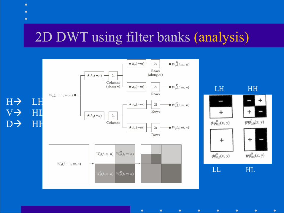
2D DWT using filter banks (analysis)
Hà LH Và HL Dà HH
LH HH
LL HL

Illustrating 2D wavelet decomposition
The wavelet transform can be applied again on the lowpass-lowpass version of the image, yielding seven subimages.
LL LH
HL HH
LL
HH
HL
LH

2D IDWT using filter banks (synthesis)
Hà LH Và HL Dà HH

Applications• Noise filtering • Image compression
– Fingerprint compression • Image fusion • Recognition G. Bebis, A. Gyaourova, S. Singh, and I. Pavlidis, "Face Recognition by
Fusing Thermal Infrared and Visible Imagery", Image and Vision Computing, vol. 24, no. 7, pp. 727-742, 2006.
• Image matching and retrieval Charles E. Jacobs Adam Finkelstein David H. Salesin, "Fast
Multiresolution Image Querying", SIGRAPH, 1995.

Image Querying
“query by content” or “query by example” !Typically, the K best matches are reported.

Fast Multiresolution Image Querying
painted low resolution target
queries