Embed Size (px)
Citation preview
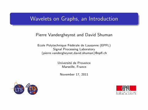
Wavelets on Graphs, an Introduction
Pierre Vandergheynst and David Shuman
Ecole Polytechnique Federale de Lausanne (EPFL)Signal Processing Laboratory
{pierre.vandergheynst,david.shuman}@epfl.ch
Universite de ProvenceMarseille, France
November 17, 2011
Intro Spectral Graph Theory Wavelets on Graphs Chebyshev Approximation Distributed Processing Open Issues
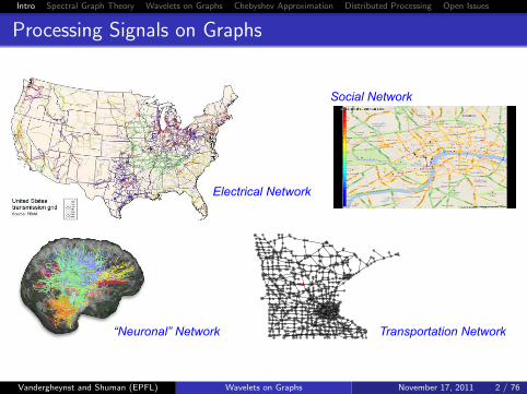
Processing Signals on GraphsProcessing Signals on Graphs
2
Electrical Network
Transportation Network“Neuronal” Network
Social Network
Vandergheynst and Shuman (EPFL) Wavelets on Graphs November 17, 2011 2 / 76
Intro Spectral Graph Theory Wavelets on Graphs Chebyshev Approximation Distributed Processing Open Issues
Outline
1 Introduction
2 Spectral Graph Theory Background� Definitions
� Differential Operators on Graphs
� Graph Laplacian Eigenvectors
� Two Applications of Graph Laplacian Eigenvectors
� Graph Downsampling
� Filtering on Graphs
3 Wavelet Constructions on Graphs
4 Approximate Graph Multiplier Operators
5 Distributed Signal Processing via the Chebyshev Approximation
6 Open Issues and Challenges
Vandergheynst and Shuman (EPFL) Wavelets on Graphs November 17, 2011 3 / 76
Intro Spectral Graph Theory Wavelets on Graphs Chebyshev Approximation Distributed Processing Open Issues
Spectral Graph Theory Notation
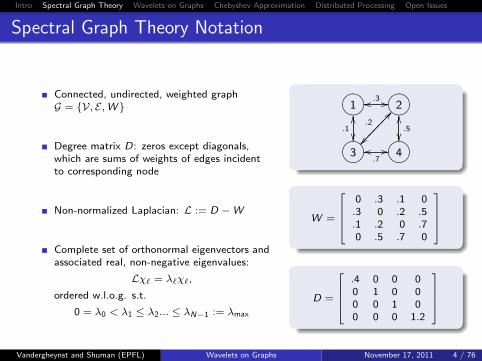
Connected, undirected, weighted graphG = {V, E,W }
Degree matrix D: zeros except diagonals,which are sums of weights of edges incidentto corresponding node
Non-normalized Laplacian: L := D −W
Complete set of orthonormal eigenvectors andassociated real, non-negative eigenvalues:
Lχ` = λ`χ`,
ordered w.l.o.g. s.t.
0 = λ0 < λ1 ≤ λ2... ≤ λN−1 := λmax
?>=<89:;1.3 //
.1��
?>=<89:;2
.5��
oo
.2
���������
?>=<89:;3
@@�������
OO
.7//?>=<89:;4
OO
oo
W =
0 .3 .1 0.3 0 .2 .5.1 .2 0 .70 .5 .7 0
D =
.4 0 0 00 1 0 00 0 1 00 0 0 1.2
Vandergheynst and Shuman (EPFL) Wavelets on Graphs November 17, 2011 4 / 76
Intro Spectral Graph Theory Wavelets on Graphs Chebyshev Approximation Distributed Processing Open Issues
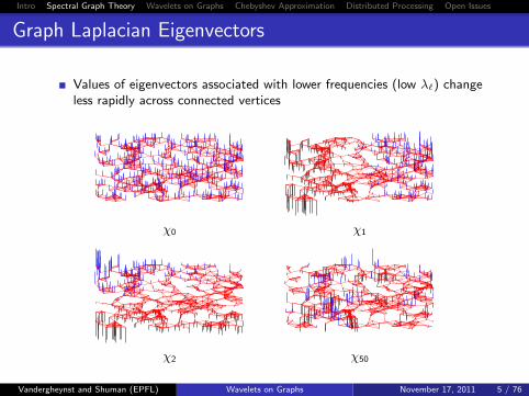
Graph Laplacian Eigenvectors
Values of eigenvectors associated with lower frequencies (low λ`) changeless rapidly across connected vertices
χ0 χ1
χ2 χ50
Vandergheynst and Shuman (EPFL) Wavelets on Graphs November 17, 2011 5 / 76
Intro Spectral Graph Theory Wavelets on Graphs Chebyshev Approximation Distributed Processing Open Issues
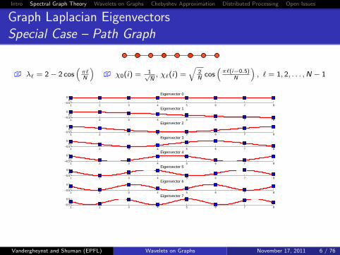
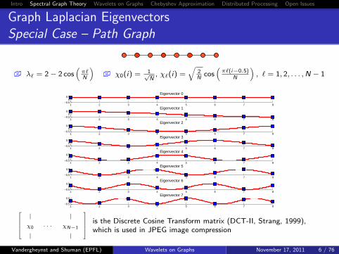
Graph Laplacian EigenvectorsSpecial Case – Path Graph
� λ` = 2− 2 cos(π`N
)� χ0(i) = 1√
N, χ`(i) =
√2N
cos(π`(i−0.5)
N
), ` = 1, 2, . . . ,N − 1
1 2 3 4 5 6 7 8−0.5
00.5
Eigenvector 0
1 2 3 4 5 6 7 8−0.5
00.5
Eigenvector 1
1 2 3 4 5 6 7 8−0.5
00.5
Eigenvector 2
1 2 3 4 5 6 7 8−0.5
00.5
Eigenvector 3
1 2 3 4 5 6 7 8−0.5
00.5
Eigenvector 4
1 2 3 4 5 6 7 8−0.5
00.5
Eigenvector 5
1 2 3 4 5 6 7 8−0.5
00.5
Eigenvector 6
1 2 3 4 5 6 7 8−0.5
00.5
Eigenvector 7
| |
χ0 · · · χN−1
| |
is the Discrete Cosine Transform matrix (DCT-II, Strang, 1999),which is used in JPEG image compression
Vandergheynst and Shuman (EPFL) Wavelets on Graphs November 17, 2011 6 / 76
Intro Spectral Graph Theory Wavelets on Graphs Chebyshev Approximation Distributed Processing Open Issues
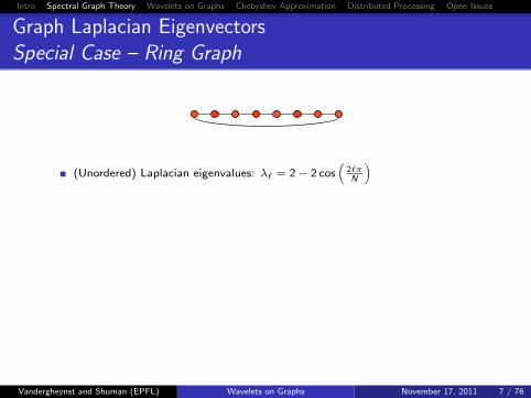
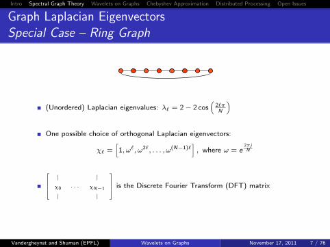
Graph Laplacian EigenvectorsSpecial Case – Ring Graph
(Unordered) Laplacian eigenvalues: λ` = 2− 2 cos(
2`πN
)
One possible choice of orthogonal Laplacian eigenvectors:
χ` =[1, ω`, ω2`, . . . , ω(N−1)`
], where ω = e
2πjN
| |
χ0 · · · χN−1
| |
is the Discrete Fourier Transform (DFT) matrix
Vandergheynst and Shuman (EPFL) Wavelets on Graphs November 17, 2011 7 / 76
Intro Spectral Graph Theory Wavelets on Graphs Chebyshev Approximation Distributed Processing Open Issues
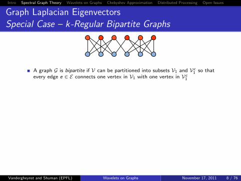
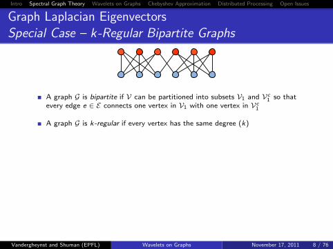
Graph Laplacian EigenvectorsSpecial Case – k-Regular Bipartite Graphs
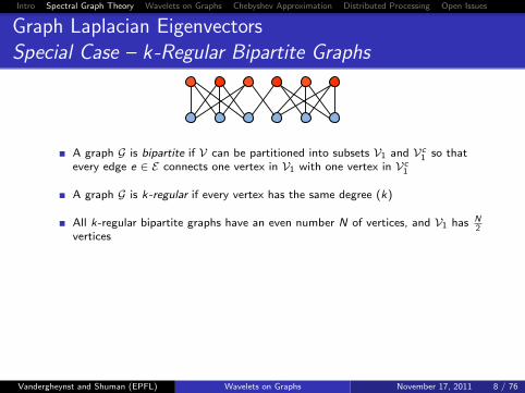
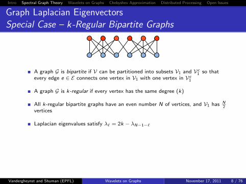
A graph G is bipartite if V can be partitioned into subsets V1 and Vc1 so that
every edge e ∈ E connects one vertex in V1 with one vertex in Vc1
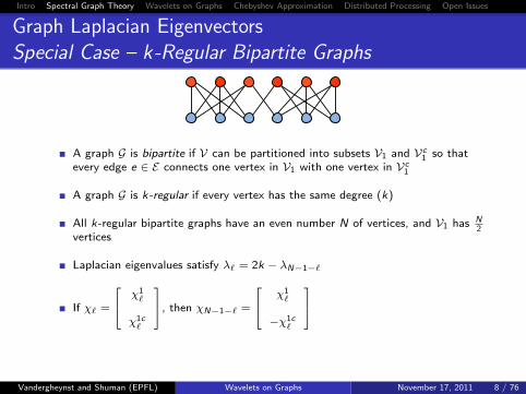
A graph G is k-regular if every vertex has the same degree (k)
All k-regular bipartite graphs have an even number N of vertices, and V1 has N2
vertices
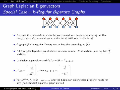
Laplacian eigenvalues satisfy λ` = 2k − λN−1−`
If χ` =
χ1`
χ1c`
, then χN−1−` =
χ1`
−χ1c`
For Lnorm, λ` = 2− λN−1−` and the Laplacian eigenvector property holds forany (non-regular) bipartite graph as well
Vandergheynst and Shuman (EPFL) Wavelets on Graphs November 17, 2011 8 / 76
Intro Spectral Graph Theory Wavelets on Graphs Chebyshev Approximation Distributed Processing Open Issues
Graph Laplacian EigenvectorsSpecial Case – k-Regular Bipartite Graphs
A graph G is bipartite if V can be partitioned into subsets V1 and Vc1 so that
every edge e ∈ E connects one vertex in V1 with one vertex in Vc1
A graph G is k-regular if every vertex has the same degree (k)
All k-regular bipartite graphs have an even number N of vertices, and V1 has N2
vertices
Laplacian eigenvalues satisfy λ` = 2k − λN−1−`
If χ` =
χ1`
χ1c`
, then χN−1−` =
χ1`
−χ1c`
For Lnorm, λ` = 2− λN−1−` and the Laplacian eigenvector property holds forany (non-regular) bipartite graph as well
Vandergheynst and Shuman (EPFL) Wavelets on Graphs November 17, 2011 8 / 76
Intro Spectral Graph Theory Wavelets on Graphs Chebyshev Approximation Distributed Processing Open Issues
Outline
1 Introduction
2 Spectral Graph Theory Background� Definitions
� Differential Operators on Graphs
� Graph Laplacian Eigenvectors
� Two Applications of Graph Laplacian Eigenvectors
� Graph Downsampling
� Filtering on Graphs
3 Wavelet Constructions on Graphs
4 Approximate Graph Multiplier Operators
5 Distributed Signal Processing via the Chebyshev Approximation
6 Open Issues and Challenges
Vandergheynst and Shuman (EPFL) Wavelets on Graphs November 17, 2011 9 / 76
Intro Spectral Graph Theory Wavelets on Graphs Chebyshev Approximation Distributed Processing Open Issues
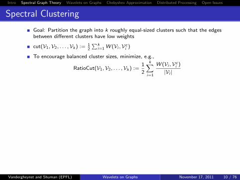
Spectral Clustering
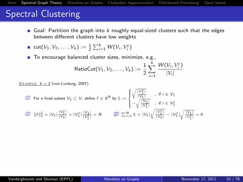
Goal: Partition the graph into k roughly equal-sized clusters such that the edgesbetween different clusters have low weights
cut(V1,V2, . . . ,Vk ) := 12
∑ki=1 W (Vi ,Vc
i )
To encourage balanced cluster sizes, minimize, e.g.,
RatioCut(V1,V2, . . . ,Vk ) :=1
2
k∑i=1
W (Vi ,Vci )
|Vi |
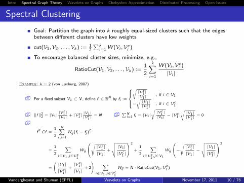
Example: k = 2 (von Luxburg, 2007)
� For a fixed subset V1 ⊂ V, define f ∈ RN by fi :=
√|Vc
1|
|V1|, if i ∈ V1
−√|V1||Vc
1| , if i ∈ Vc
1
� ‖f ‖22 = |V1|
|Vc1 ||V1|
+ |Vc1 ||V1||Vc
1| = N �
∑Ni=1 fi = |V1|
√|Vc
1|
|V1|− |Vc
1 |√|V1||Vc
1| = 0
�
fTLf =1
2
N∑i,j=1
Wij (fi − fj )2
=1
2
∑i∈V1,j∈Vc
1
Wij
√ |Vc1 ||V1|
+
√√√√ |V1||Vc
1 |
2
+1
2
∑i∈Vc
1,j∈V1
Wij
−√ |Vc1 ||V1|
−
√√√√ |V1||Vc
1 |
2
=
(|V1||Vc
1 |+|Vc
1 ||V1|
+ 2
) ∑i∈V1,j∈Vc
1
Wij = N · RatioCut(V1,Vc1 )
Vandergheynst and Shuman (EPFL) Wavelets on Graphs November 17, 2011 10 / 76
Intro Spectral Graph Theory Wavelets on Graphs Chebyshev Approximation Distributed Processing Open Issues
Spectral Clustering
Goal: Partition the graph into k roughly equal-sized clusters such that the edgesbetween different clusters have low weights
cut(V1,V2, . . . ,Vk ) := 12
∑ki=1 W (Vi ,Vc
i )
To encourage balanced cluster sizes, minimize, e.g.,
RatioCut(V1,V2, . . . ,Vk ) :=1
2
k∑i=1
W (Vi ,Vci )
|Vi |
Example: k = 2 (von Luxburg, 2007)
� For a fixed subset V1 ⊂ V, define f ∈ RN by fi :=
√|Vc
1|
|V1|, if i ∈ V1
−√|V1||Vc
1| , if i ∈ Vc
1
� ‖f ‖22 = |V1|
|Vc1 ||V1|
+ |Vc1 ||V1||Vc
1| = N �
∑Ni=1 fi = |V1|
√|Vc
1|
|V1|− |Vc
1 |√|V1||Vc
1| = 0
�
fTLf =1
2
N∑i,j=1
Wij (fi − fj )2
=1
2
∑i∈V1,j∈Vc
1
Wij
√ |Vc1 ||V1|
+
√√√√ |V1||Vc
1 |
2
+1
2
∑i∈Vc
1,j∈V1
Wij
−√ |Vc1 ||V1|
−
√√√√ |V1||Vc
1 |
2
=
(|V1||Vc
1 |+|Vc
1 ||V1|
+ 2
) ∑i∈V1,j∈Vc
1
Wij = N · RatioCut(V1,Vc1 )
Vandergheynst and Shuman (EPFL) Wavelets on Graphs November 17, 2011 10 / 76
Intro Spectral Graph Theory Wavelets on Graphs Chebyshev Approximation Distributed Processing Open Issues
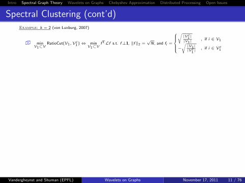
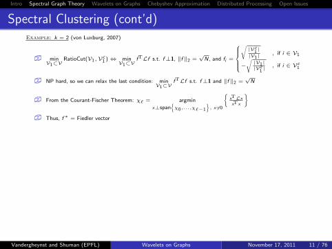
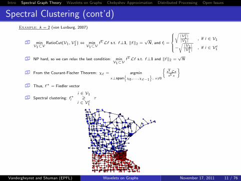
Spectral Clustering (cont’d)Example: k = 2 (von Luxburg, 2007)
� minV1⊂V
RatioCut(V1,Vc1 )⇔ min
V1⊂VfTLf s.t. f⊥1, ‖f ‖2 =
√N, and fi =
√|Vc
1|
|V1|, if i ∈ V1
−√|V1||Vc
1| , if i ∈ Vc
1
� NP hard, so we can relax the last condition: minV1⊂V
fTLf s.t. f⊥1 and ‖f ‖2 =√
N
� From the Courant-Fischer Theorem: χ` = argmin
x⊥span{χ0,...,χ`−1
}, x 6=0
{xTLxxTx
}
� Thus, f ∗ = Fiedler vector
� Spectral clustering: f ∗i
i ∈ V1≷
i ∈ Vc1
τ
Vandergheynst and Shuman (EPFL) Wavelets on Graphs November 17, 2011 11 / 76
Intro Spectral Graph Theory Wavelets on Graphs Chebyshev Approximation Distributed Processing Open Issues
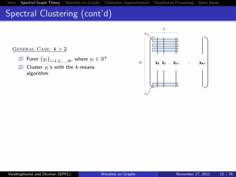
Spectral Clustering (cont’d)
General Case: k > 2
� Form {yi}i=1,2,...,N , where yi ∈ Rk
� Cluster yi ’s with the k-meansalgorithm
k
N χ0 χ1 χk-1 χN-1 … …
yn
y1
Vandergheynst and Shuman (EPFL) Wavelets on Graphs November 17, 2011 12 / 76
Intro Spectral Graph Theory Wavelets on Graphs Chebyshev Approximation Distributed Processing Open Issues
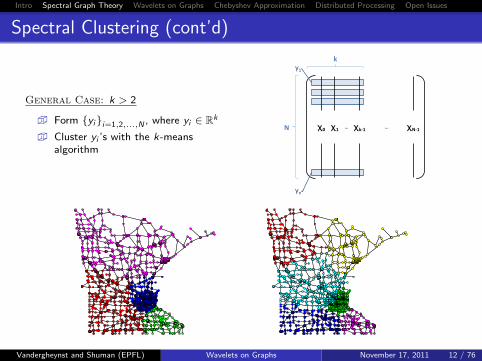
Spectral Clustering (cont’d)
General Case: k > 2
� Form {yi}i=1,2,...,N , where yi ∈ Rk
� Cluster yi ’s with the k-meansalgorithm
k
N χ0 χ1 χk-1 χN-1 … …
yn
y1
Vandergheynst and Shuman (EPFL) Wavelets on Graphs November 17, 2011 12 / 76
Intro Spectral Graph Theory Wavelets on Graphs Chebyshev Approximation Distributed Processing Open Issues
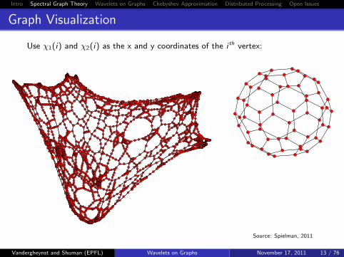
Graph Visualization
Use χ1(i) and χ2(i) as the x and y coordinates of the i th vertex:
Source: Spielman, 2011
Vandergheynst and Shuman (EPFL) Wavelets on Graphs November 17, 2011 13 / 76
Intro Spectral Graph Theory Wavelets on Graphs Chebyshev Approximation Distributed Processing Open Issues
Outline
1 Introduction
2 Spectral Graph Theory Background� Definitions
� Differential Operators on Graphs
� Graph Laplacian Eigenvectors
� Two Applications of Graph Laplacian Eigenvectors
� Graph Downsampling
� Filtering on Graphs
3 Wavelet Constructions on Graphs
4 Approximate Graph Multiplier Operators
5 Distributed Signal Processing via the Chebyshev Approximation
6 Open Issues and Challenges
Vandergheynst and Shuman (EPFL) Wavelets on Graphs November 17, 2011 14 / 76
Intro Spectral Graph Theory Wavelets on Graphs Chebyshev Approximation Distributed Processing Open Issues
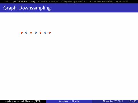
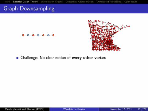
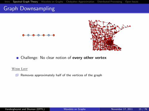
Graph Downsampling
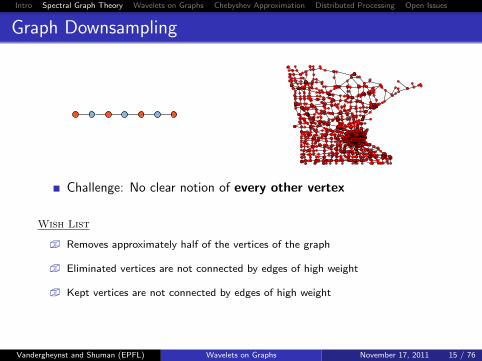
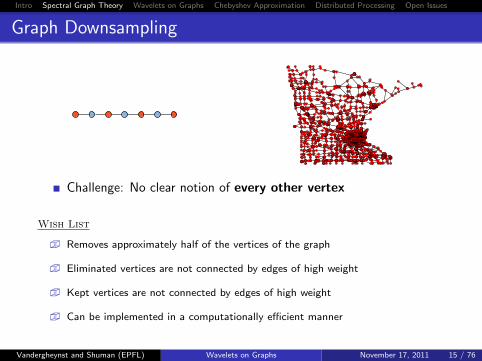
Challenge: No clear notion of every other vertex
Wish List
� Removes approximately half of the vertices of the graph
� Eliminated vertices are not connected by edges of high weight
� Kept vertices are not connected by edges of high weight
� Can be implemented in a computationally efficient manner
Vandergheynst and Shuman (EPFL) Wavelets on Graphs November 17, 2011 15 / 76
Intro Spectral Graph Theory Wavelets on Graphs Chebyshev Approximation Distributed Processing Open Issues
Graph Downsampling
Challenge: No clear notion of every other vertex
Wish List
� Removes approximately half of the vertices of the graph
� Eliminated vertices are not connected by edges of high weight
� Kept vertices are not connected by edges of high weight
� Can be implemented in a computationally efficient manner
Vandergheynst and Shuman (EPFL) Wavelets on Graphs November 17, 2011 15 / 76
Intro Spectral Graph Theory Wavelets on Graphs Chebyshev Approximation Distributed Processing Open Issues
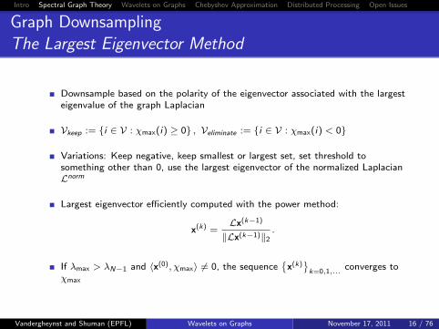
Graph DownsamplingThe Largest Eigenvector Method
Downsample based on the polarity of the eigenvector associated with the largesteigenvalue of the graph Laplacian
Vkeep := {i ∈ V : χmax(i) ≥ 0} , Veliminate := {i ∈ V : χmax(i) < 0}
Variations: Keep negative, keep smallest or largest set, set threshold tosomething other than 0, use the largest eigenvector of the normalized LaplacianLnorm
Largest eigenvector efficiently computed with the power method:
x(k) =Lx(k−1)
‖Lx(k−1)‖2.
If λmax > λN−1 and 〈x(0), χmax〉 6= 0, the sequence{
x(k)}
k=0,1,...converges to
χmax
Vandergheynst and Shuman (EPFL) Wavelets on Graphs November 17, 2011 16 / 76
Intro Spectral Graph Theory Wavelets on Graphs Chebyshev Approximation Distributed Processing Open Issues
Graph DownsamplingThe Largest Eigenvector Method – Examples
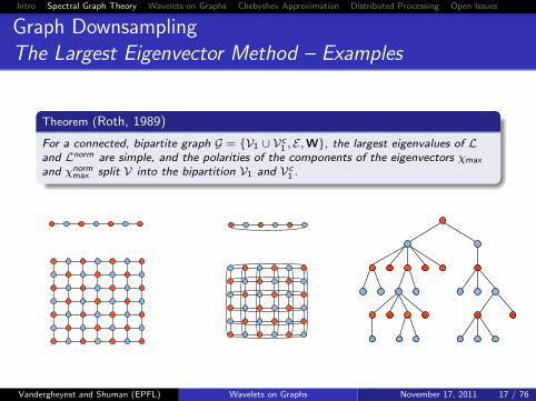
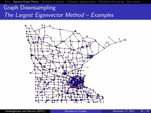
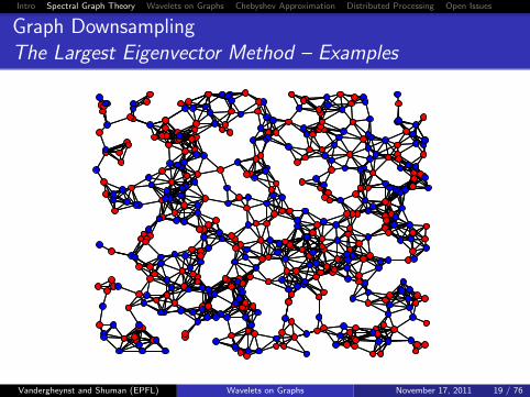
Theorem (Roth, 1989)
For a connected, bipartite graph G = {V1 ∪ Vc1 , E,W}, the largest eigenvalues of L
and Lnorm are simple, and the polarities of the components of the eigenvectors χmax
and χnormmax split V into the bipartition V1 and Vc
1 .
Vandergheynst and Shuman (EPFL) Wavelets on Graphs November 17, 2011 17 / 76
Intro Spectral Graph Theory Wavelets on Graphs Chebyshev Approximation Distributed Processing Open Issues
Graph DownsamplingThe Largest Eigenvector Method – Examples
Vandergheynst and Shuman (EPFL) Wavelets on Graphs November 17, 2011 18 / 76
Intro Spectral Graph Theory Wavelets on Graphs Chebyshev Approximation Distributed Processing Open Issues
Graph DownsamplingThe Largest Eigenvector Method – Examples
Vandergheynst and Shuman (EPFL) Wavelets on Graphs November 17, 2011 19 / 76
Intro Spectral Graph Theory Wavelets on Graphs Chebyshev Approximation Distributed Processing Open Issues
Graph DownsamplingConnections with Graph Coloring and Spectral Clustering
A graph G = {V, E,W} is k-colorable if there exists a partition of V into subsetsV1,V2, . . . ,Vk such that if i ∼ j , then i and j are in different subsets in thepartition
The chromatic number C of a graph G is the smallest k such that G isk-colorable
The chromatic number is equal to 2 if and only if the graph is bipartite
In graph downsampling, we are interested in finding an approximate 2-coloringwith few edges connecting vertices in the same subsets
In some sense dual to the spectral clustering problem
Vandergheynst and Shuman (EPFL) Wavelets on Graphs November 17, 2011 20 / 76
Intro Spectral Graph Theory Wavelets on Graphs Chebyshev Approximation Distributed Processing Open Issues
Graph DownsamplingConnections with Nodal Domains
+0 –– +
–
+
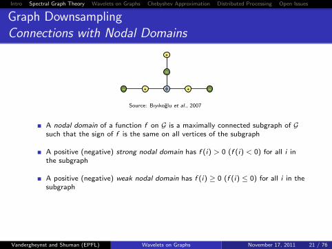
Source: Bıyıkoglu et al., 2007
A nodal domain of a function f on G is a maximally connected subgraph of Gsuch that the sign of f is the same on all vertices of the subgraph
A positive (negative) strong nodal domain has f (i) > 0 (f (i) < 0) for all i inthe subgraph
A positive (negative) weak nodal domain has f (i) ≥ 0 (f (i) ≤ 0) for all i in thesubgraph
# weak nodal domains of f on G ≤ # strong nodal domains of f on G
Graph downsampling is closely related to the problem of maximizing the numberof nodal domains
Vandergheynst and Shuman (EPFL) Wavelets on Graphs November 17, 2011 21 / 76
Intro Spectral Graph Theory Wavelets on Graphs Chebyshev Approximation Distributed Processing Open Issues
Graph DownsamplingConnections with Nodal Domains
+0 –– +
–
+
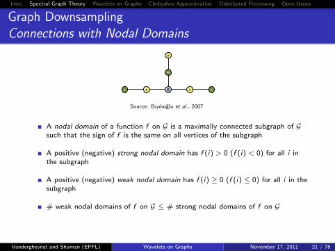
Source: Bıyıkoglu et al., 2007
A nodal domain of a function f on G is a maximally connected subgraph of Gsuch that the sign of f is the same on all vertices of the subgraph
A positive (negative) strong nodal domain has f (i) > 0 (f (i) < 0) for all i inthe subgraph
A positive (negative) weak nodal domain has f (i) ≥ 0 (f (i) ≤ 0) for all i in thesubgraph
# weak nodal domains of f on G ≤ # strong nodal domains of f on G
Graph downsampling is closely related to the problem of maximizing the numberof nodal domains
Vandergheynst and Shuman (EPFL) Wavelets on Graphs November 17, 2011 21 / 76
Intro Spectral Graph Theory Wavelets on Graphs Chebyshev Approximation Distributed Processing Open Issues
Graph DownsamplingConnections with Nodal Domains
+0 –– +
–
+
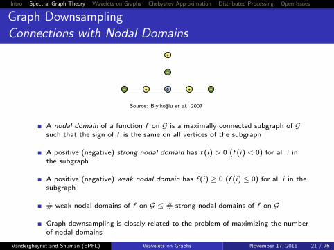
Source: Bıyıkoglu et al., 2007
A nodal domain of a function f on G is a maximally connected subgraph of Gsuch that the sign of f is the same on all vertices of the subgraph
A positive (negative) strong nodal domain has f (i) > 0 (f (i) < 0) for all i inthe subgraph
A positive (negative) weak nodal domain has f (i) ≥ 0 (f (i) ≤ 0) for all i in thesubgraph
# weak nodal domains of f on G ≤ # strong nodal domains of f on G
Graph downsampling is closely related to the problem of maximizing the numberof nodal domains
Vandergheynst and Shuman (EPFL) Wavelets on Graphs November 17, 2011 21 / 76
Intro Spectral Graph Theory Wavelets on Graphs Chebyshev Approximation Distributed Processing Open Issues
Graph DownsamplingConnections with Nodal Domains (cont’d)
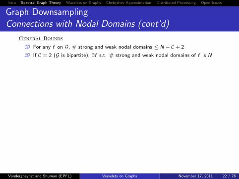
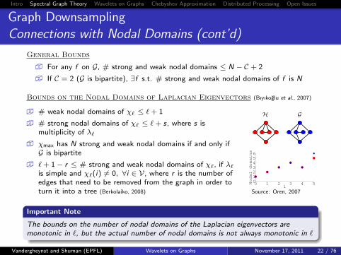
General Bounds
� For any f on G, # strong and weak nodal domains ≤ N − C + 2
� If C = 2 (G is bipartite), ∃f s.t. # strong and weak nodal domains of f is N
Bounds on the Nodal Domains of Laplacian Eigenvectors (Bıyıkoglu et al., 2007)
� # weak nodal domains of χ` ≤ `+ 1
� # strong nodal domains of χ` ≤ `+ s, where s ismultiplicity of λ`
� χmax has N strong and weak nodal domains if and only ifG is bipartite
� `+ 1− r ≤ # strong and weak nodal domains of χ`, if λ`is simple and χ`(i) 6= 0, ∀i ∈ V, where r is the number ofedges that need to be removed from the graph in order toturn it into a tree (Berkolaiko, 2008)
H G
H
0 1 2 3 4 50123456
l
Nodal domains
Source: Oren, 2007
Important Note
The bounds on the number of nodal domains of the Laplacian eigenvectors aremonotonic in `, but the actual number of nodal domains is not always monotonic in `
Vandergheynst and Shuman (EPFL) Wavelets on Graphs November 17, 2011 22 / 76
Intro Spectral Graph Theory Wavelets on Graphs Chebyshev Approximation Distributed Processing Open Issues
Graph DownsamplingConnections with Nodal Domains (cont’d)
General Bounds
� For any f on G, # strong and weak nodal domains ≤ N − C + 2
� If C = 2 (G is bipartite), ∃f s.t. # strong and weak nodal domains of f is N
Bounds on the Nodal Domains of Laplacian Eigenvectors (Bıyıkoglu et al., 2007)
� # weak nodal domains of χ` ≤ `+ 1
� # strong nodal domains of χ` ≤ `+ s, where s ismultiplicity of λ`
� χmax has N strong and weak nodal domains if and only ifG is bipartite
� `+ 1− r ≤ # strong and weak nodal domains of χ`, if λ`is simple and χ`(i) 6= 0, ∀i ∈ V, where r is the number ofedges that need to be removed from the graph in order toturn it into a tree (Berkolaiko, 2008)
H G
H
0 1 2 3 4 50123456
l
Nodal domains
Source: Oren, 2007
Important Note
The bounds on the number of nodal domains of the Laplacian eigenvectors aremonotonic in `, but the actual number of nodal domains is not always monotonic in `
Vandergheynst and Shuman (EPFL) Wavelets on Graphs November 17, 2011 22 / 76
Intro Spectral Graph Theory Wavelets on Graphs Chebyshev Approximation Distributed Processing Open Issues
Filtering on Graphs
Filtering: represent an input signal as a combination of othersignals, and amplify or attenuate the contributions of some of thecomponent signals
In classical signal processing, the most common choice of basis isthe complex exponentials, which results in frequency filtering
Not difficult to extend this notion to signals on graphs via theeigenvectors of the graph Laplacian
Vandergheynst and Shuman (EPFL) Wavelets on Graphs November 17, 2011 23 / 76
Intro Spectral Graph Theory Wavelets on Graphs Chebyshev Approximation Distributed Processing Open Issues
Graph Fourier Transform
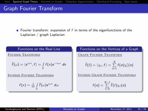
Fourier transform: expansion of f in terms of the eigenfunctions of theLaplacian / graph Laplacian
Functions on the Real Line
Fourier Transform
f (ω) = 〈e iωx , f 〉 =∫R
f (x)e−iωx dx
Inverse Fourier Transform
f (x) = 12π
∫R
f (ω)e iωx dω
Functions on the Vertices of a Graph
Graph Fourier Transform
f (`) = 〈χ`, f 〉 =N∑
n=1
f (n)χ∗` (n)
Inverse Graph Fourier Transform
f (n) =N−1∑
=0
f (`)χ`(n)
Vandergheynst and Shuman (EPFL) Wavelets on Graphs November 17, 2011 24 / 76
Intro Spectral Graph Theory Wavelets on Graphs Chebyshev Approximation Distributed Processing Open Issues
Fourier Multiplier Operator (Filter)
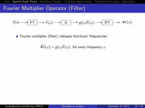
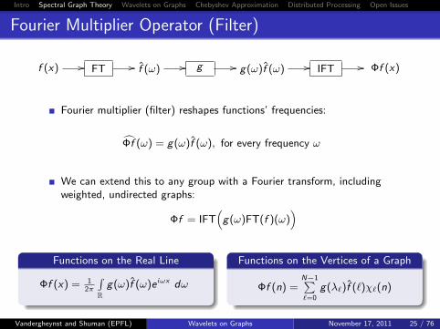
f (x) // FT // f (ω) // g // g(ω)f (ω) // IFT // Φf (x)
Fourier multiplier (filter) reshapes functions’ frequencies:
Φf (ω) = g(ω)f (ω), for every frequency ω
We can extend this to any group with a Fourier transform, includingweighted, undirected graphs:
Φf = IFT(g(ω)FT(f )(ω)
)
Functions on the Real Line
Φf (x) = 12π
∫R
g(ω)f (ω)e iωx dω
Functions on the Vertices of a Graph
Φf (n) =N−1∑
=0
g(λ`)f (`)χ`(n)
Vandergheynst and Shuman (EPFL) Wavelets on Graphs November 17, 2011 25 / 76
Intro Spectral Graph Theory Wavelets on Graphs Chebyshev Approximation Distributed Processing Open Issues
Fourier Multiplier Operator (Filter)
f (x) // FT // f (ω) // g // g(ω)f (ω) // IFT // Φf (x)
Fourier multiplier (filter) reshapes functions’ frequencies:
Φf (ω) = g(ω)f (ω), for every frequency ω
We can extend this to any group with a Fourier transform, includingweighted, undirected graphs:
Φf = IFT(g(ω)FT(f )(ω)
)
Functions on the Real Line
Φf (x) = 12π
∫R
g(ω)f (ω)e iωx dω
Functions on the Vertices of a Graph
Φf (n) =N−1∑
=0
g(λ`)f (`)χ`(n)
Vandergheynst and Shuman (EPFL) Wavelets on Graphs November 17, 2011 25 / 76
Intro Spectral Graph Theory Wavelets on Graphs Chebyshev Approximation Distributed Processing Open Issues
Generalized Graph Multiplier Operators
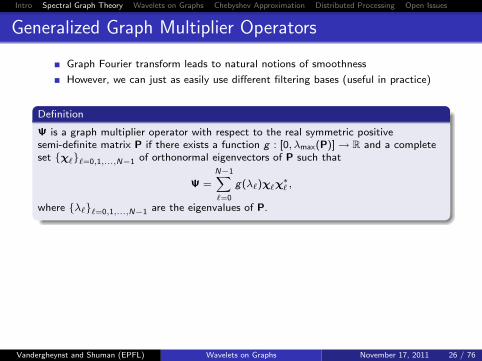
Graph Fourier transform leads to natural notions of smoothness
However, we can just as easily use different filtering bases (useful in practice)
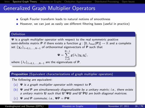
Definition
Ψ is a graph multiplier operator with respect to the real symmetric positivesemi-definite matrix P if there exists a function g : [0, λmax(P)]→ R and a completeset {χ`}`=0,1,...,N−1 of orthonormal eigenvectors of P such that
Ψ =
N−1∑`=0
g(λ`)χ`χ∗` ,
where {λ`}`=0,1,...,N−1 are the eigenvalues of P.
Proposition (Equivalent characterizations of graph multiplier operators)
The following are equivalent:
(a) Ψ is a graph multiplier operator with respect to P.
(b) Ψ and P are simultaneously diagonalizable by a unitary matrix; i.e., there existsa unitary matrix U such that U∗ΨU and U∗PU are both diagonal matrices.
(c) Ψ and P commute; i.e., ΨP = PΨ.
Vandergheynst and Shuman (EPFL) Wavelets on Graphs November 17, 2011 26 / 76
Intro Spectral Graph Theory Wavelets on Graphs Chebyshev Approximation Distributed Processing Open Issues
Generalized Graph Multiplier Operators
Graph Fourier transform leads to natural notions of smoothness
However, we can just as easily use different filtering bases (useful in practice)
Definition
Ψ is a graph multiplier operator with respect to the real symmetric positivesemi-definite matrix P if there exists a function g : [0, λmax(P)]→ R and a completeset {χ`}`=0,1,...,N−1 of orthonormal eigenvectors of P such that
Ψ =
N−1∑`=0
g(λ`)χ`χ∗` ,
where {λ`}`=0,1,...,N−1 are the eigenvalues of P.
Proposition (Equivalent characterizations of graph multiplier operators)
The following are equivalent:
(a) Ψ is a graph multiplier operator with respect to P.
(b) Ψ and P are simultaneously diagonalizable by a unitary matrix; i.e., there existsa unitary matrix U such that U∗ΨU and U∗PU are both diagonal matrices.
(c) Ψ and P commute; i.e., ΨP = PΨ.
Vandergheynst and Shuman (EPFL) Wavelets on Graphs November 17, 2011 26 / 76
Intro Spectral Graph Theory Wavelets on Graphs Chebyshev Approximation Distributed Processing Open Issues
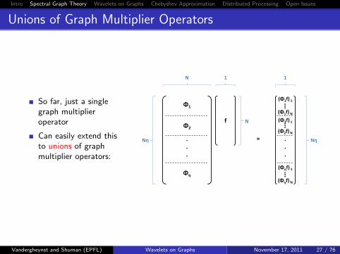
Unions of Graph Multiplier Operators
So far, just a singlegraph multiplieroperator
Can easily extend thisto unions of graphmultiplier operators:
(Φηf) 1
f
(Φ1f) 1
Φ2
Φη
1N 1
NηNη
N
=...
…
(Φ1f) N
Φ1
…
(Φηf) N
.
.
.
(Φ2f) 1
(Φ2f) N
…
Vandergheynst and Shuman (EPFL) Wavelets on Graphs November 17, 2011 27 / 76
Intro Spectral Graph Theory Wavelets on Graphs Chebyshev Approximation Distributed Processing Open Issues
Outline
1 Introduction
2 Spectral Graph Theory Background
3 Wavelet Constructions on Graphs
4 Approximate Graph Multiplier Operators
5 Distributed Signal Processing via the Chebyshev Approximation
6 Open Issues and Challenges
Vandergheynst and Shuman (EPFL) Wavelets on Graphs November 17, 2011 28 / 76
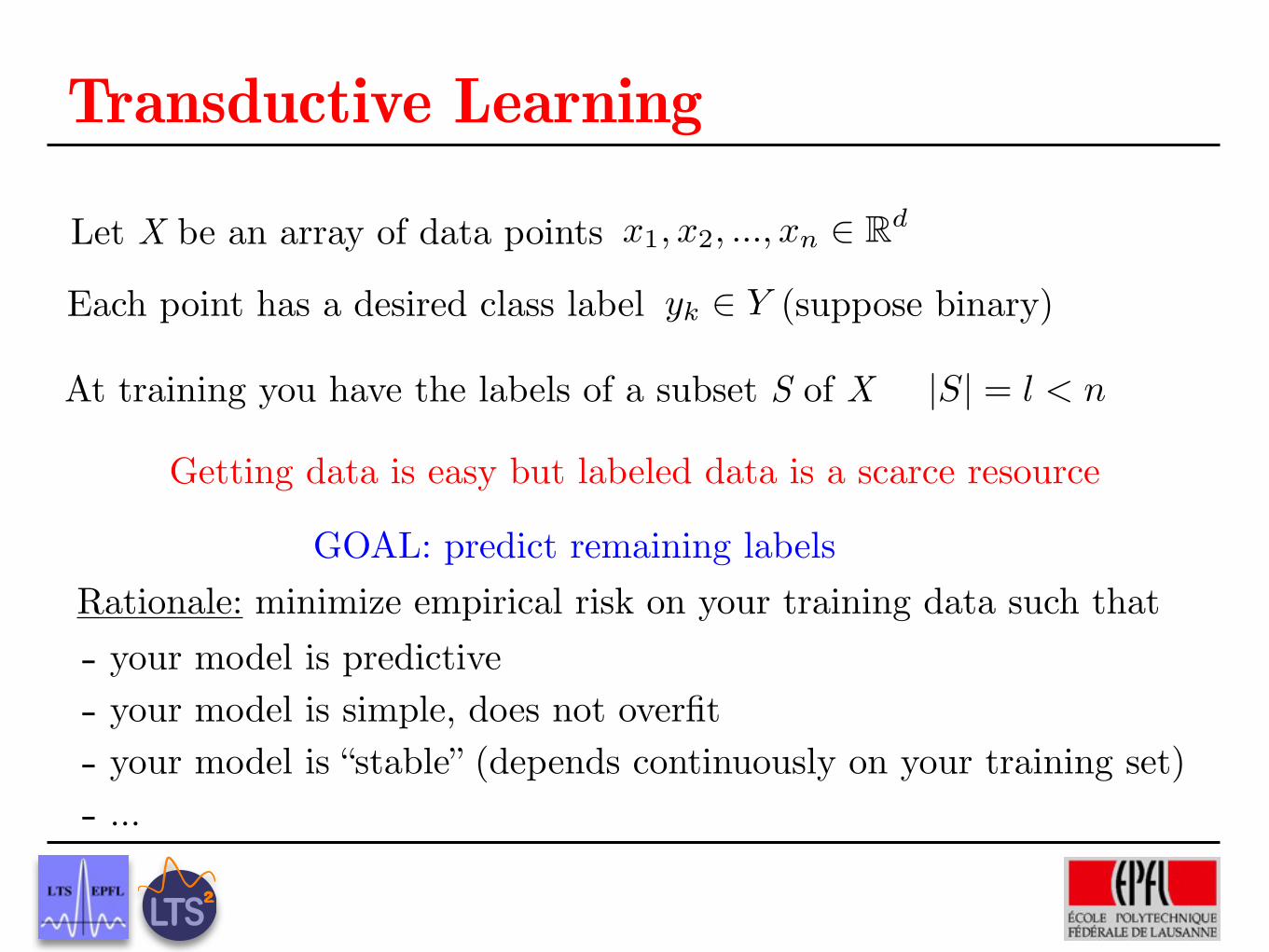
Each point has a desired class label (suppose binary)
x1, x2, ..., xn 2 Rd
|S| = l < n
Transductive Learning
Let X be an array of data points
yk 2 Y
At training you have the labels of a subset S of X
GOAL: predict remaining labelsRationale: minimize empirical risk on your training data such that- your model is predictive- your model is simple, does not overfit- your model is “stable” (depends continuously on your training set)- ...
Getting data is easy but labeled data is a scarce resource
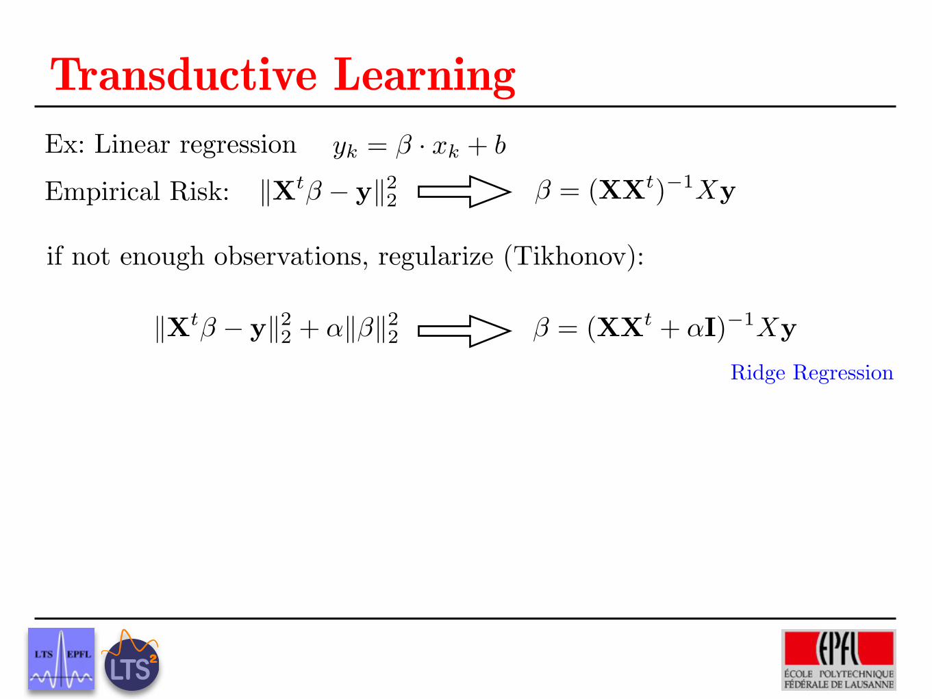
kXt� � yk22
yk = � · xk + b
� = (XXt)�1Xy
� = (XXt + ↵I)�1XykXt� � yk22 + ↵k�k2
2
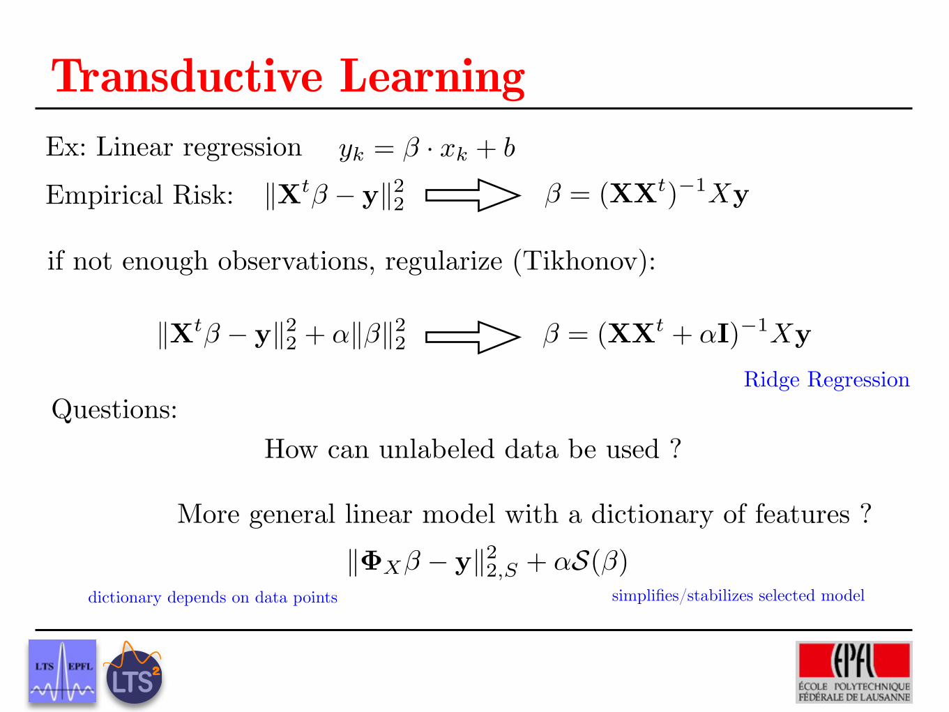
Transductive LearningEx: Linear regressionEmpirical Risk:
if not enough observations, regularize (Tikhonov):
Ridge Regression
kXt� � yk22
yk = � · xk + b
� = (XXt)�1Xy
� = (XXt + ↵I)�1XykXt� � yk22 + ↵k�k2
2
Transductive LearningEx: Linear regressionEmpirical Risk:
if not enough observations, regularize (Tikhonov):
Ridge Regression
k�X� � yk22,S + ↵S(�)
How can unlabeled data be used ?Questions:
More general linear model with a dictionary of features ?
dictionary depends on data points simplifies/stabilizes selected model
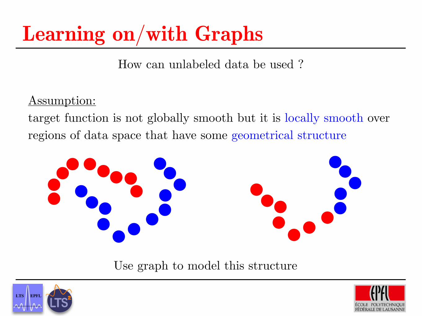
Learning on/with GraphsHow can unlabeled data be used ?
Assumption: target function is not globally smooth but it is locally smooth over regions of data space that have some geometrical structure
Use graph to model this structure
�f =X
i,j2X
Wij(f(xi)� f(xj))2
= f tLf
kXtS� � yk2
2 + ↵k�k22 + ��tXLXt�
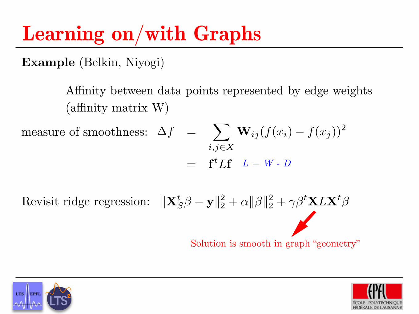
Learning on/with GraphsExample (Belkin, Niyogi)
Affinity between data points represented by edge weights (affinity matrix W)
measure of smoothness:
Revisit ridge regression:
L = W - D
Solution is smooth in graph “geometry”
�X
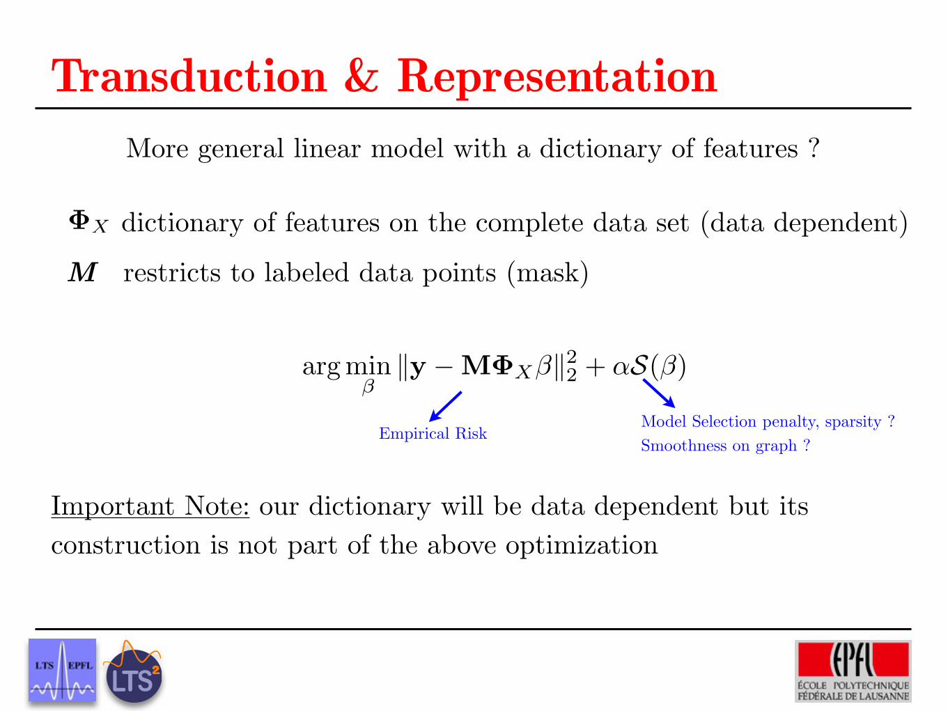
arg min�ky �M�X�k2
2 + ↵S(�)
Transduction & RepresentationMore general linear model with a dictionary of features ?
dictionary of features on the complete data set (data dependent)
M restricts to labeled data points (mask)
Empirical RiskModel Selection penalty, sparsity ?Smoothness on graph ?
Important Note: our dictionary will be data dependent but its construction is not part of the above optimization
�s,a(x) =1s�
�x� a
s
⇥
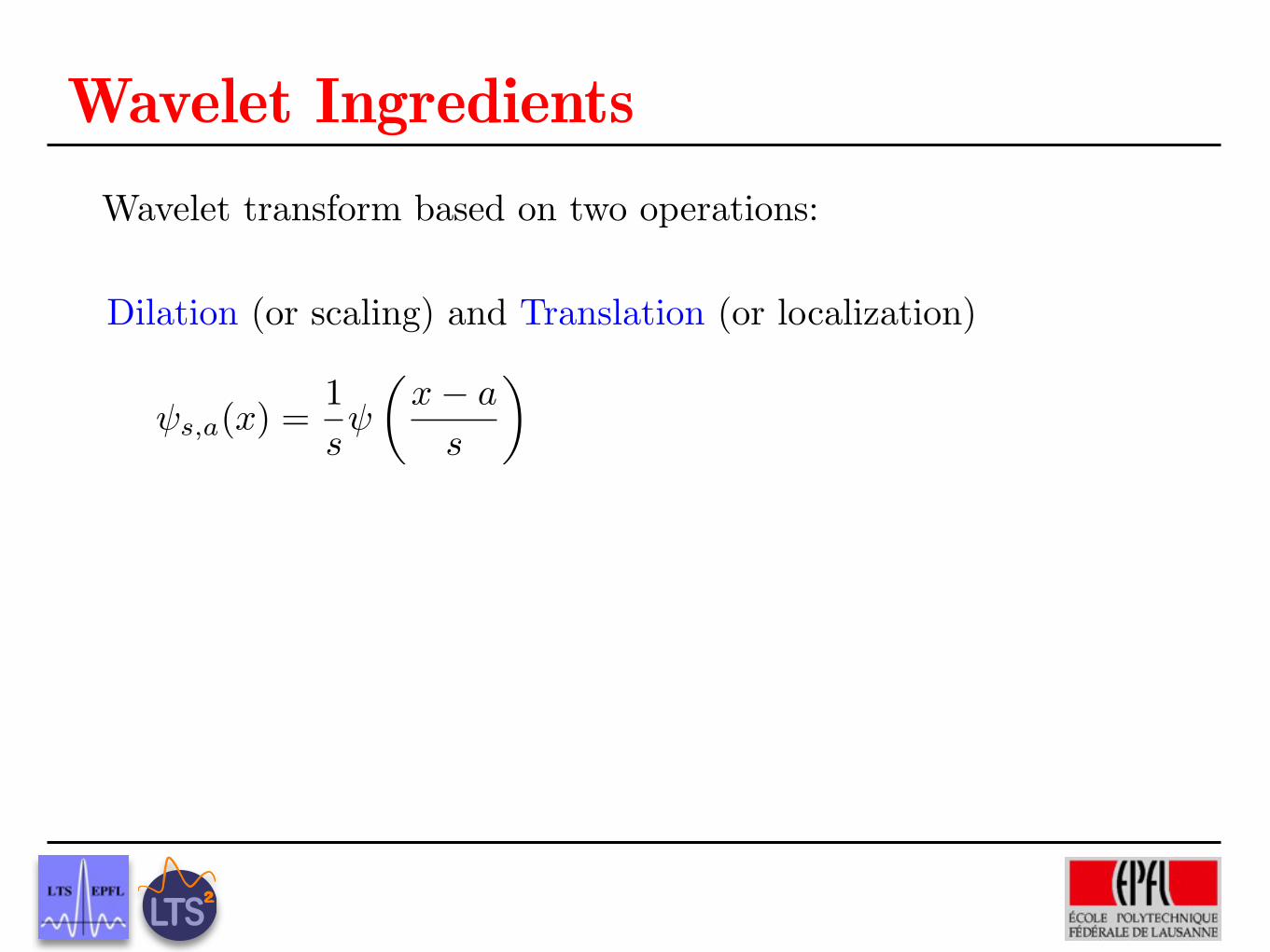
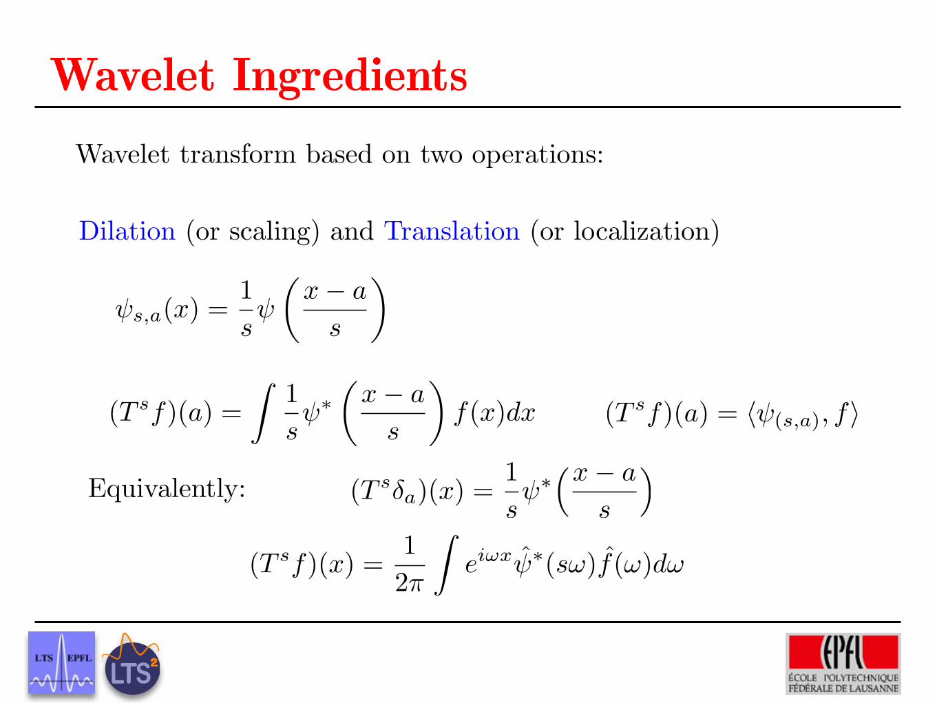
Wavelet IngredientsWavelet transform based on two operations:
Dilation (or scaling) and Translation (or localization)
�s,a(x) =1s�
�x� a
s
⇥
(T sf)(a) =⇤
1s��
�x� a
s
⇥f(x)dx (T sf)(a) = ��(s,a), f⇥
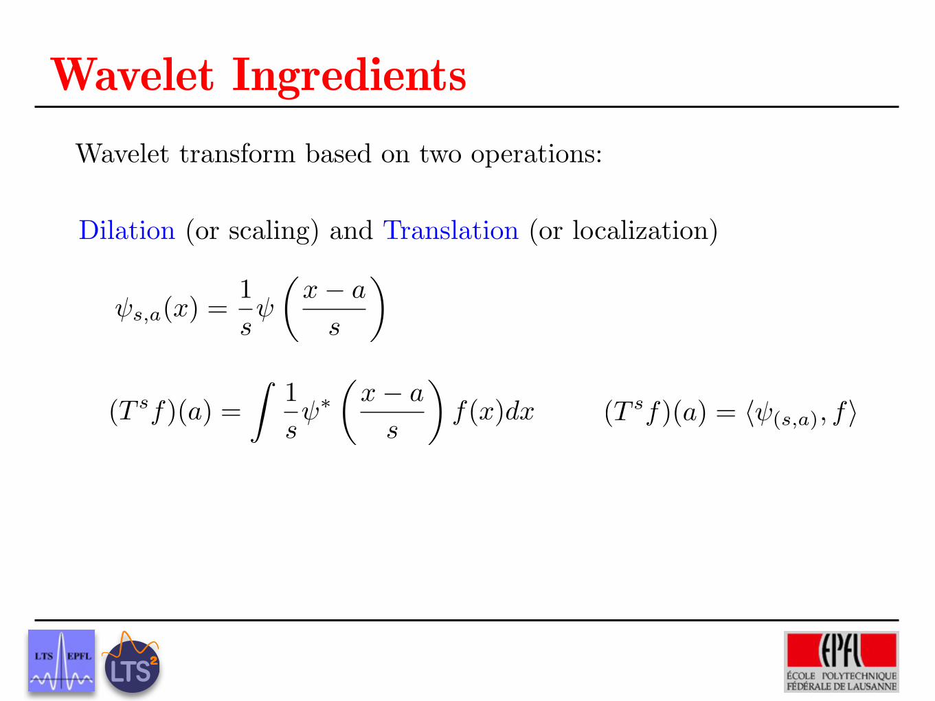
Wavelet IngredientsWavelet transform based on two operations:
Dilation (or scaling) and Translation (or localization)
�s,a(x) =1s�
�x� a
s
⇥
(T sf)(a) =⇤
1s��
�x� a
s
⇥f(x)dx (T sf)(a) = ��(s,a), f⇥
Wavelet IngredientsWavelet transform based on two operations:
Dilation (or scaling) and Translation (or localization)
(T s�a)(x) =1s⇥�
�x� a
s
⇥
(T sf)(x) =12�
�ei�x⇥�(s⇤)f(⇤)d⇤
Equivalently:
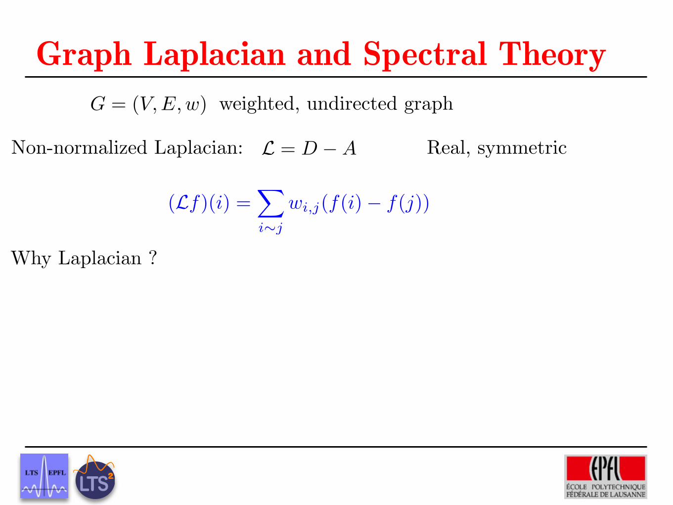
L = D �A
(Lf)(i) =�
i�j
wi,j(f(i)� f(j))
G = (V,E, w)
Graph Laplacian and Spectral Theory
Non-normalized Laplacian: Real, symmetric
Why Laplacian ?
weighted, undirected graph
L = D �A
(Lf)(i) =�
i�j
wi,j(f(i)� f(j))
G = (V,E, w)
Graph Laplacian and Spectral Theory
Non-normalized Laplacian: Real, symmetric
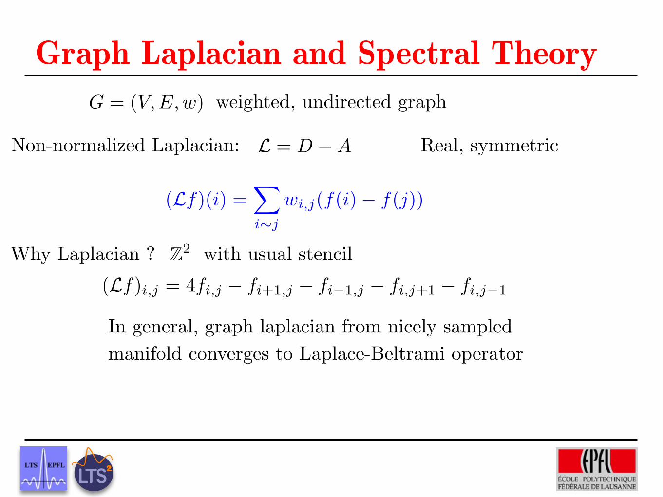
Why Laplacian ? Z2
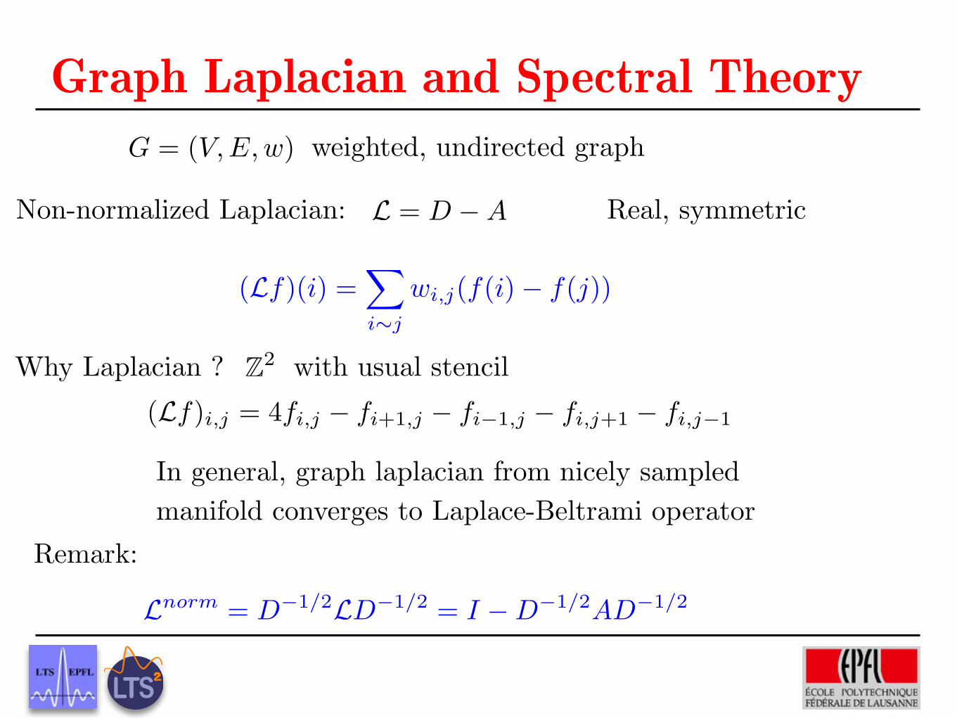
(Lf)i,j = 4fi,j � fi+1,j � fi�1,j � fi,j+1 � fi,j�1
with usual stencil
In general, graph laplacian from nicely sampled manifold converges to Laplace-Beltrami operator
weighted, undirected graph
L = D �A
(Lf)(i) =�
i�j
wi,j(f(i)� f(j))
G = (V,E, w)
Graph Laplacian and Spectral Theory
Non-normalized Laplacian: Real, symmetric
Lnorm = D�1/2LD�1/2 = I �D�1/2AD�1/2
Remark:
Why Laplacian ? Z2
(Lf)i,j = 4fi,j � fi+1,j � fi�1,j � fi,j+1 � fi,j�1
with usual stencil
In general, graph laplacian from nicely sampled manifold converges to Laplace-Beltrami operator
weighted, undirected graph
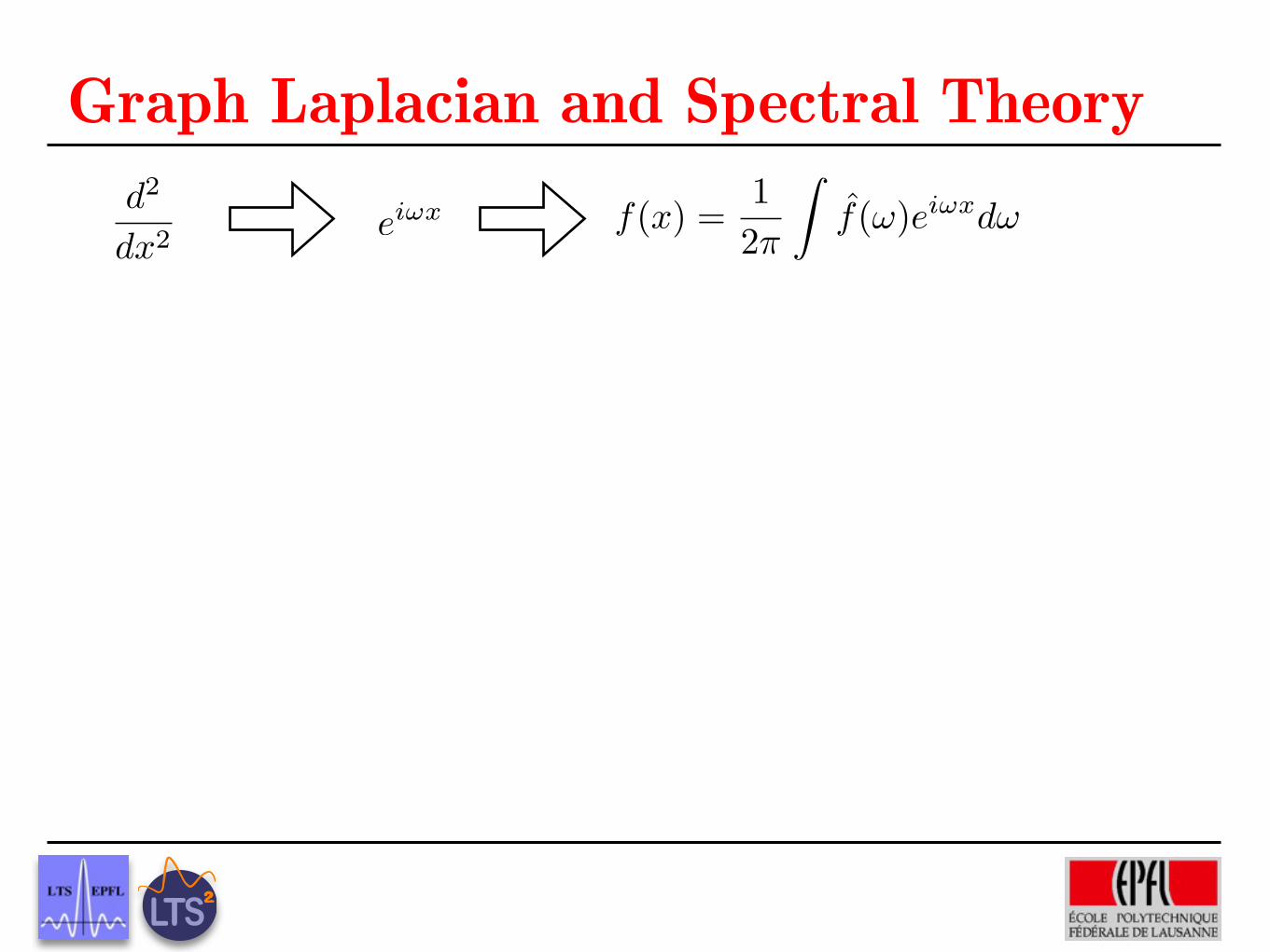
ei�x f(x) =12�
�f(⇥)ei�xd⇥
d2
dx2
Graph Laplacian and Spectral Theory
ei�x f(x) =12�
�f(⇥)ei�xd⇥
d2
dx2
Graph Laplacian and Spectral Theory
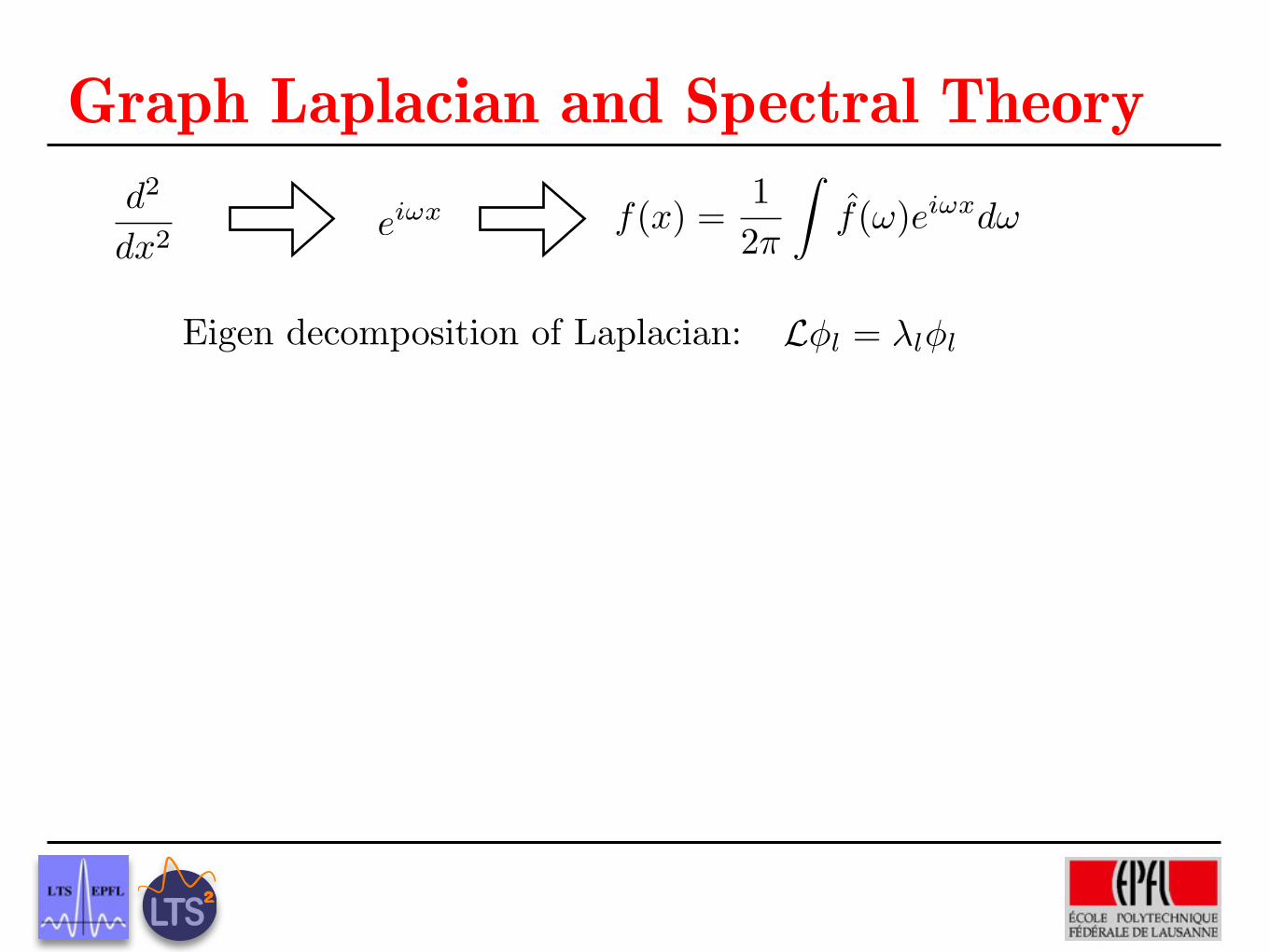
L⇥l = �l⇥lEigen decomposition of Laplacian:
ei�x f(x) =12�
�f(⇥)ei�xd⇥
d2
dx2
Graph Laplacian and Spectral Theory
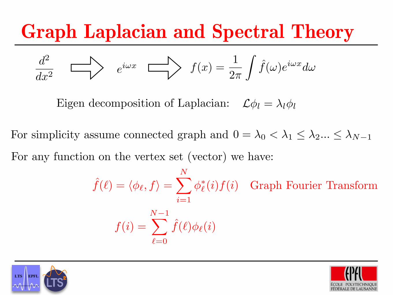
L⇥l = �l⇥lEigen decomposition of Laplacian:
0 = �0 < �1 � �2... � �N�1
f(⇤) = ��⇥, f⇥ =N�
i=1
��⇥ (i)f(i)
f(i) =N�1�
⇥=0
f(⇥)�⇥(i)
Graph Fourier Transform
For simplicity assume connected graph and
For any function on the vertex set (vector) we have:
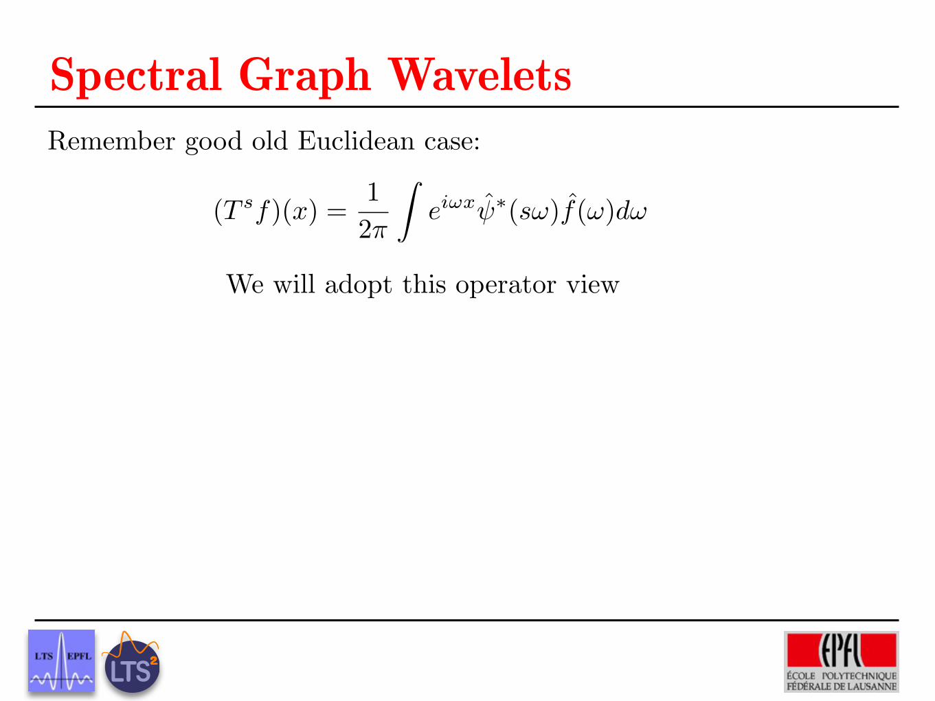
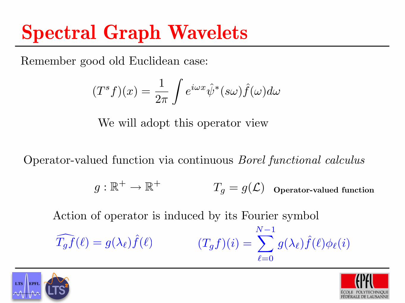
Spectral Graph WaveletsRemember good old Euclidean case:
(T sf)(x) =12�
�ei�x⇥�(s⇤)f(⇤)d⇤
We will adopt this operator view
Spectral Graph WaveletsRemember good old Euclidean case:
(T sf)(x) =12�
�ei�x⇥�(s⇤)f(⇤)d⇤
We will adopt this operator view
g : R+ � R+ Tg = g(L)
�Tgf(⇤) = g(��)f(⇤) (Tgf)(i) =N�1�
⇥=0
g(�⇥)f(⌅)⇥⇥(i)
Operator-valued function via continuous Borel functional calculus
Operator-valued function
Action of operator is induced by its Fourier symbol
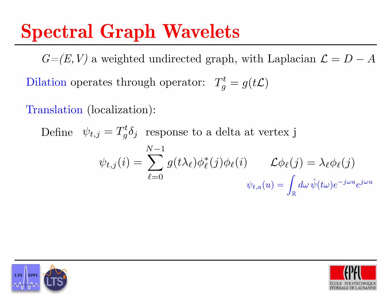
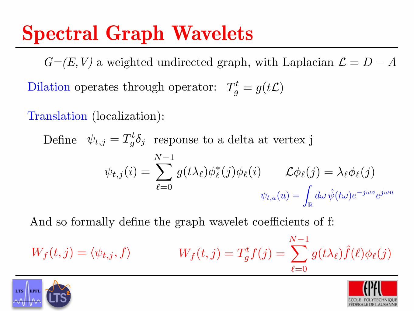
Spectral Graph WaveletsL = D �AG=(E,V) a weighted undirected graph, with Laplacian
Spectral Graph Wavelets
T tg = g(tL)Dilation operates through operator:
L = D �AG=(E,V) a weighted undirected graph, with Laplacian
Spectral Graph Wavelets
T tg = g(tL)Dilation operates through operator:
L�`(j) = �`�`(j)
⇥t,j = T tg�j
⇤t,j(i) =N�1�
⇤=0
g(t�⇤)⇥⇥⇤ (j)⇥⇤(i)
�t,a(u) =�
Rd⇥ �(t⇥)e�j�aej�u
Translation (localization):
Define response to a delta at vertex j
L = D �AG=(E,V) a weighted undirected graph, with Laplacian
Spectral Graph Wavelets
T tg = g(tL)Dilation operates through operator:
L�`(j) = �`�`(j)
⇥t,j = T tg�j
⇤t,j(i) =N�1�
⇤=0
g(t�⇤)⇥⇥⇤ (j)⇥⇤(i)
�t,a(u) =�
Rd⇥ �(t⇥)e�j�aej�u
Translation (localization):
Define response to a delta at vertex j
Wf (t, j) = ��t,j , f⇥ Wf (t, j) = T tgf(j) =
N�1�
⇥=0
g(t�⇥)f(⌃)⇥⇥(j)
And so formally define the graph wavelet coefficients of f:
L = D �AG=(E,V) a weighted undirected graph, with Laplacian
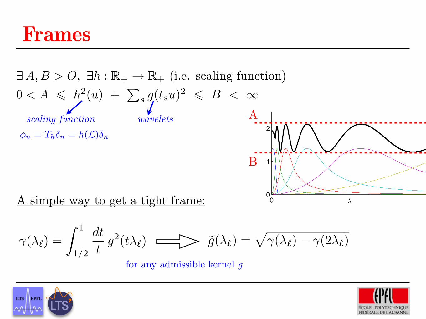
�(�`) =Z 1
1/2
dt
tg2(t�`) g(�`) =
p�(�`)� �(2�`)
�n = Th�n = h(L)�n
Frames
9A, B > O, 9h : R+ ! R+ (i.e. scaling function)
0 < A 6 h2(u) +
Ps g(tsu)
2 6 B < 1
scaling function wavelets
0 100
1
2
!
A
B
A simple way to get a tight frame:
for any admissible kernel g
−1 0 1−10
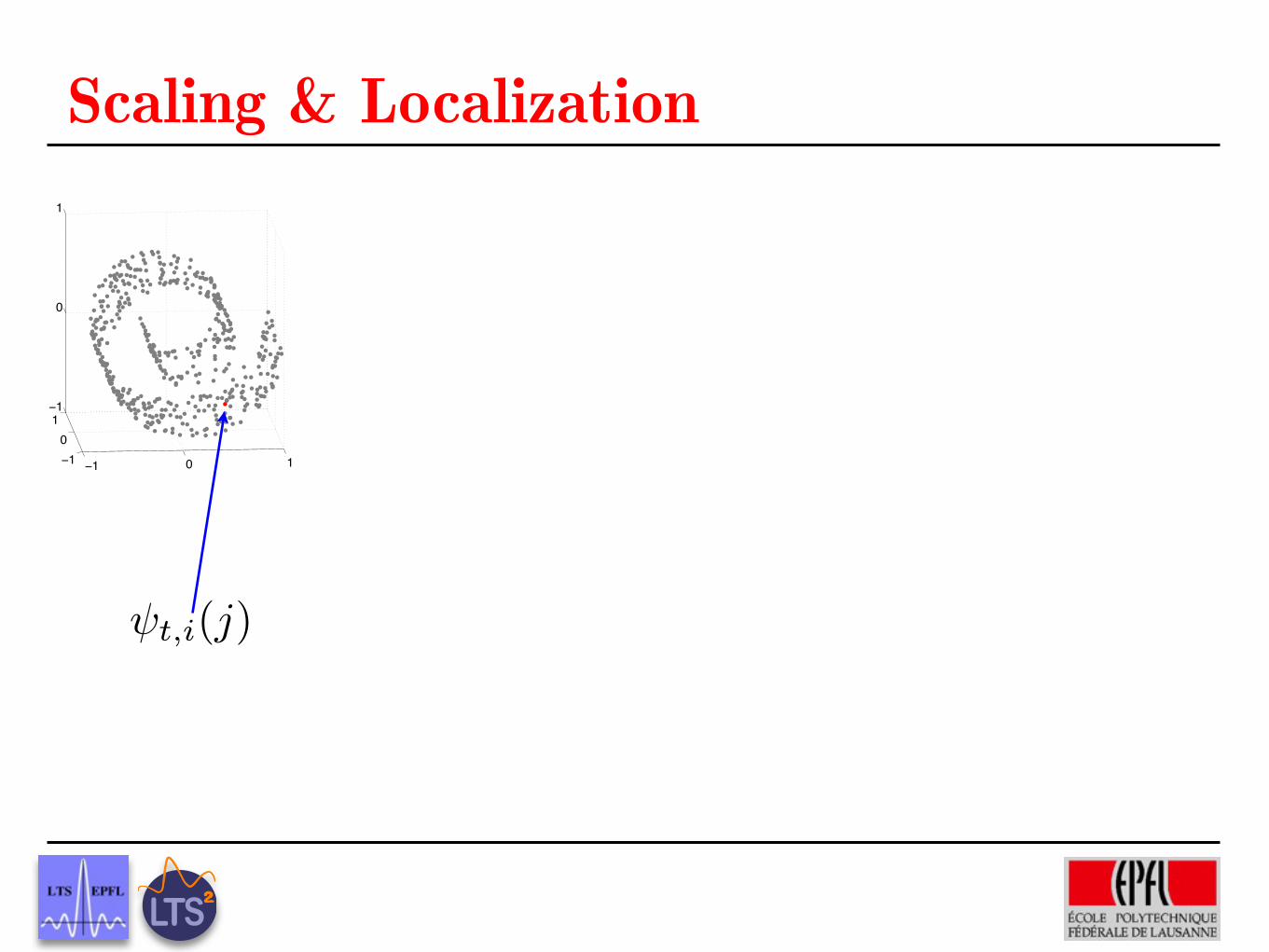
1−1
0
1
t,i(j)
Scaling & Localization
−1 0 1−10
1−1
0
1
t,i(j)
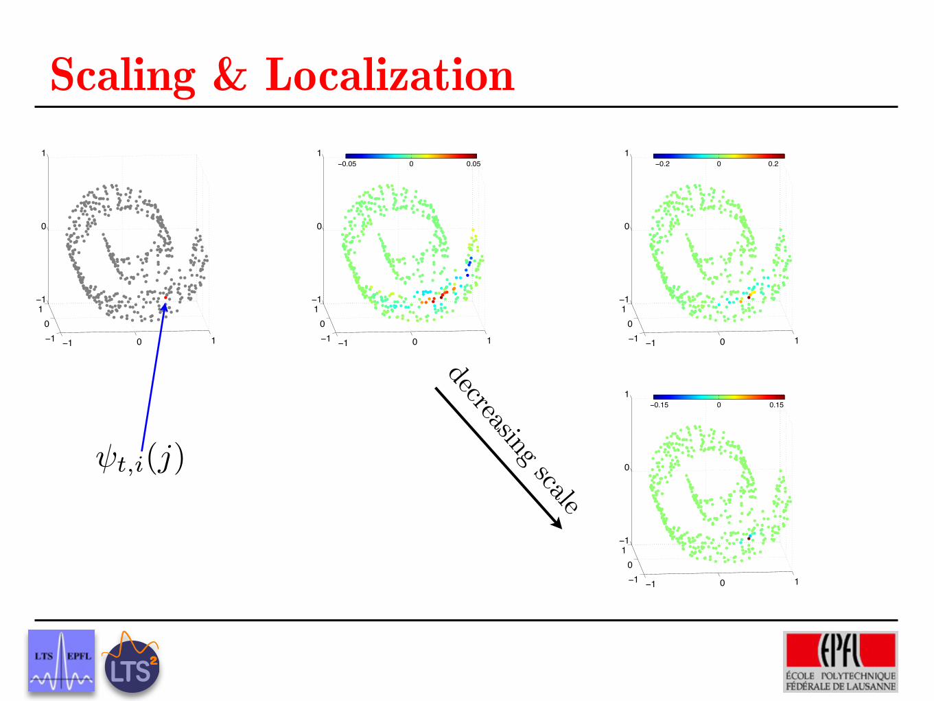
Scaling & Localization
−1 0 1−10
1−1
0
1
−0.05 0 0.05
−1 0 1−10
1−1
0
1
−0.2 0 0.2
−1 0 1−10
1−1
0
1
−0.15 0 0.15
decreasing scale
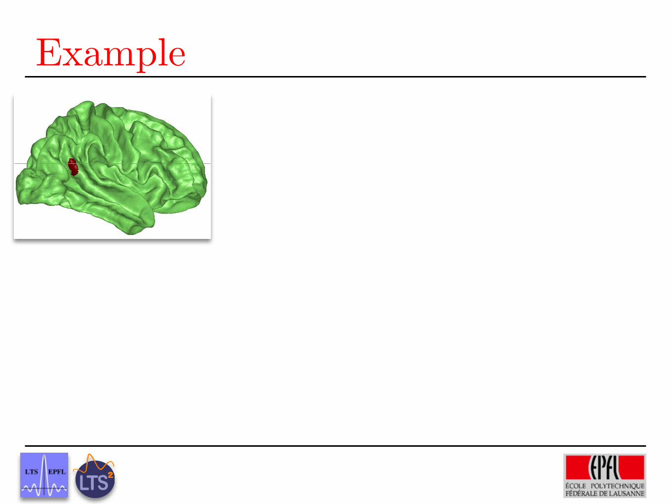
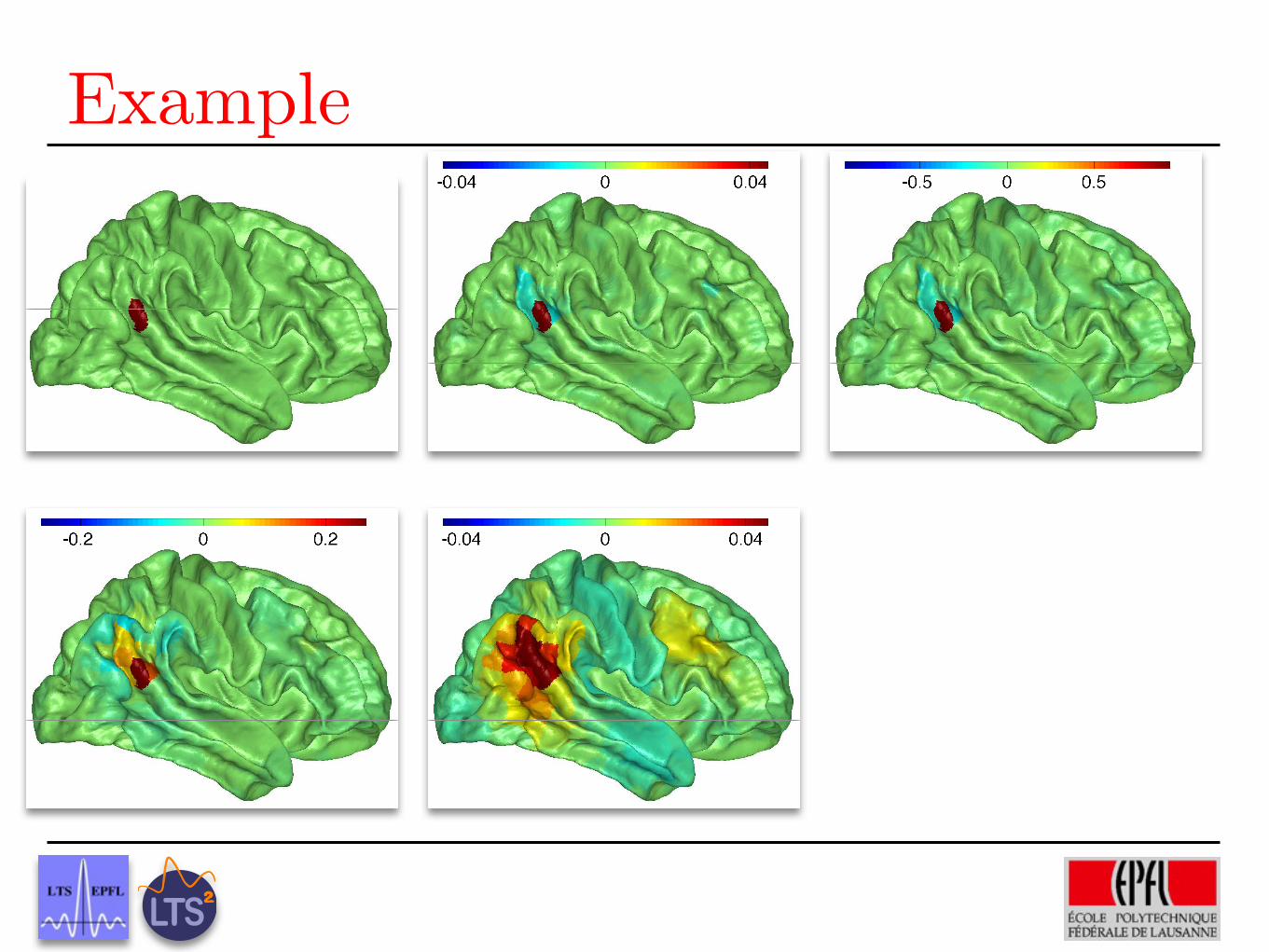
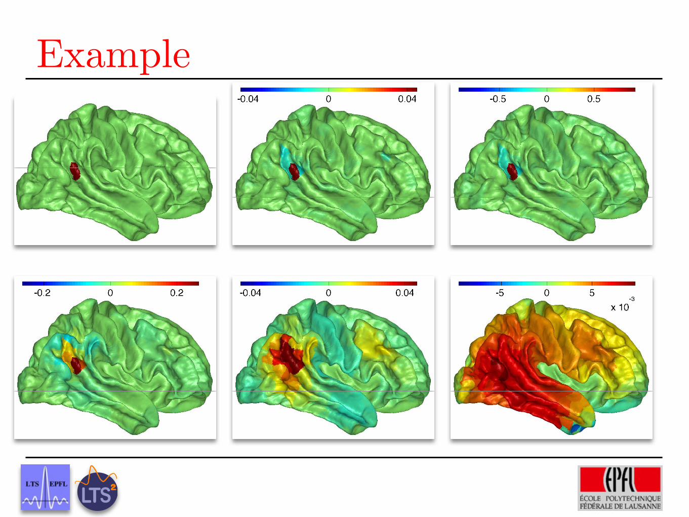
Example
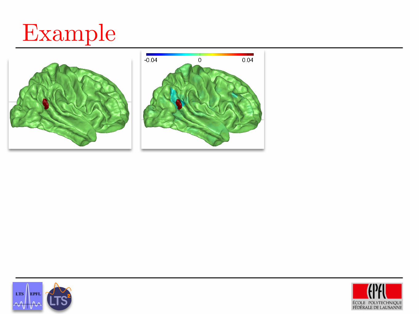
Example
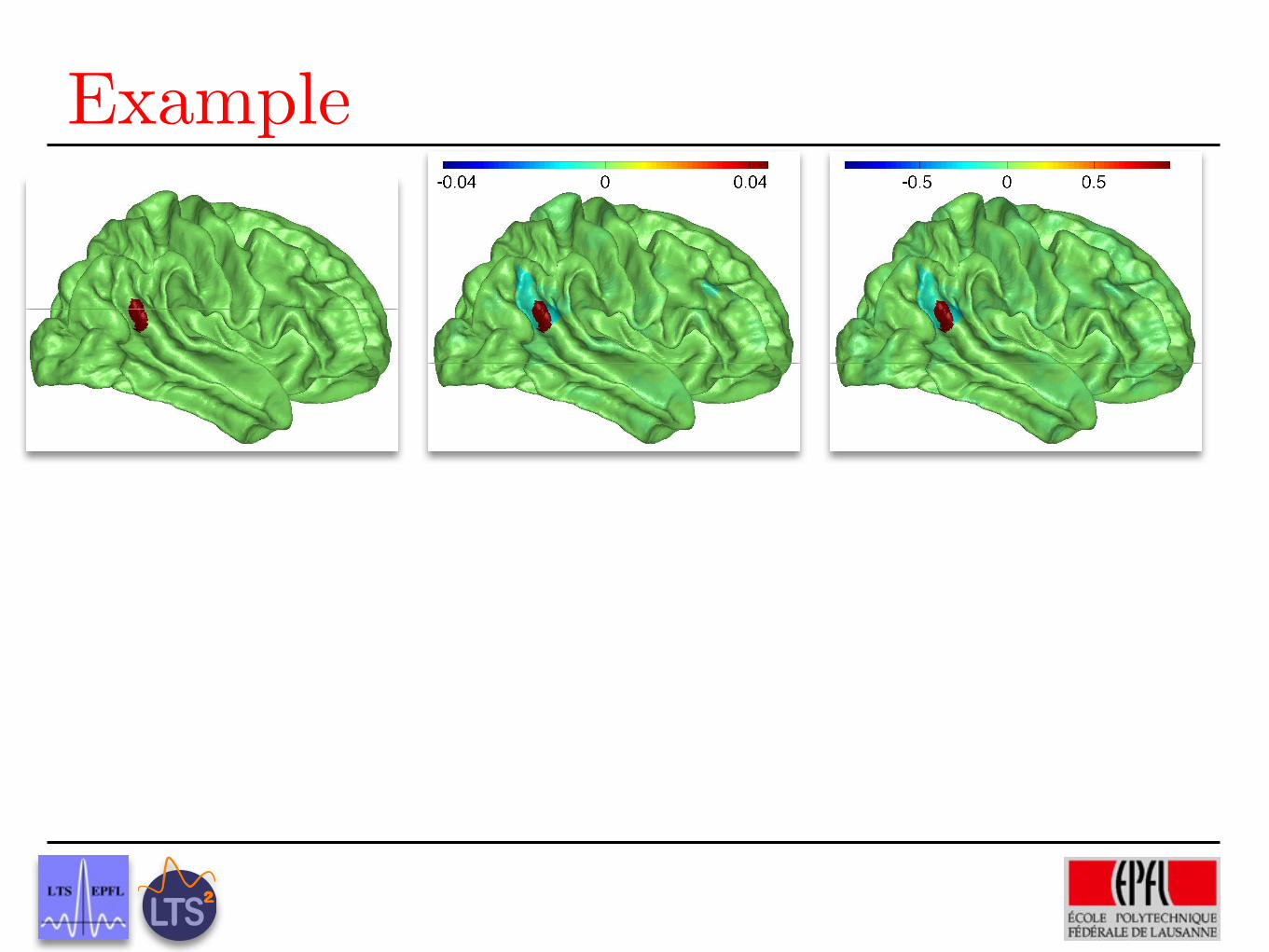
Example
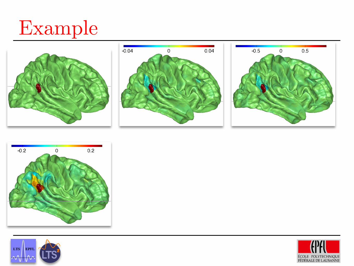
Example
Example
Example
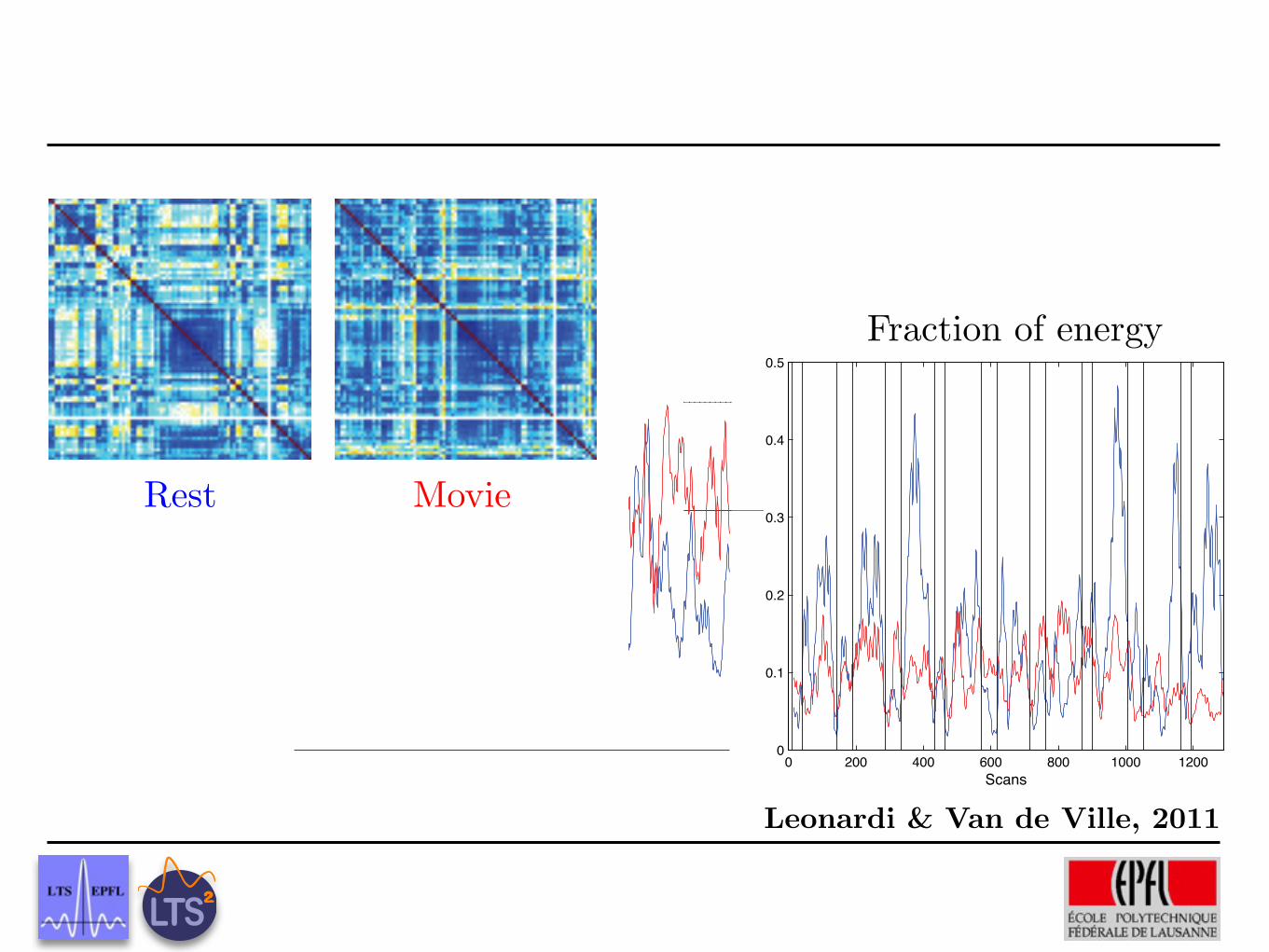
Fig. 1. Signed Laplacian matrices L for 90-region functionalconnectivity graphs during resting (left) and movies condition(right). Warm colors represent positive entries, cold colorsnegative ones; degree capped at 1 to enhance visibility.
3. RESULTS
3.1. Functional Connectivity Graph
We used fMRI data acquired from one subject during al-ternating resting and movies conditions on a 3T scan-ner (TR/TE/FA = 1.1s/27ms/90!, matrix = 64!64, voxelsize = 3.75!3.75!4.2mm3, 21 contiguous transverse slices,1.05mm gap, 2598 volumes) [11]. After realignment, fMRIdata was parcellated into 90 regions according to the Auto-mated Anatomical Labeling (AAL) atlas and regional meantime series were extracted. The time series correspondingto the same condition (rest or movies) were then concate-nated and each one decomposed using the discrete wavelettransform. Pair-wise interregional correlations between thewavelet coefficients at the different scales were estimated.The resulting 90 ! 90 correlation matrices can be inter-preted as functional connectivity in a specific frequency band[12, 13]. We used both the resting and movies correlation ma-trices obtained from the low-frequency interval 0.03-0.06Hz(scale 4) for our further analyses. The adjacency matrix A isobtained by setting the diagonal to 0 (i.e., removing loops).Fig. 1 shows the Laplacian matrices L for the resting andmovies condition, respectively.
3.2. Scaling Function and Wavelet Kernels
The scaling function and wavelet generating kernels for J =3 scales, and the eigenvalues of L are shown in Fig. 2. It in-dicates that, overall, the connectivity is increased during themovies condition (larger eigenvalues than for the resting con-dition) and that the number of eigenvalues at each scale tj iscomparable between the two conditions.
3.3. Decomposing the FMRI Signal Using the SGWT
For the decomposition, we used the original regional timecourses f that alternated between the resting and movies con-dition, that is, before concatenation. We normalized f ateach scan to remove variations in global energy between thetwo conditions and minimize effects of scanner drifts and
0 5 10 15 20 25 30 35 40 45 50ï0.5
0
0.5
1
0 5 10 15 20 25 30 35 40ï0.5
0
0.5
1
Fig. 2. Scaling function h(!) (blue curve), wavelet kernelsg(t!!), frame bound (black dotted line) and eigenvalues ofthe Laplacian matrices L (black spikes) for the resting (top)and movies condition (bottom).
movements artifacts (i.e., ||f ||2 = 1 for each scan). Wedecomposed f using both the SGWT constructed from the”resting connectivity graph” (resting frame) and the SGWTconstructed from the ”movies connectivity graph” (moviesframe). Fig. 3 shows the sum of the energy of the waveletcoefficients over all brain regions at each scan after applyinga moving average of length 24, in accordance with temporalscale 4. At the finest scale, we can see that, during the rest-ing conditions, the energy of the wavelet coefficients in theresting frame is smaller than in the movies frame (i.e., blueline below red line) (Table 1). This relation is reversed dur-ing the movies block, where the energy of the coefficients inthe movies frame is smaller (red line below blue line). Atthe coarse scale the behavior is reversed: during the rest-ing conditions, the energy of the resting-frame coefficientsis lager than that of the movies-frame coefficients (i.e., blueline above red line), whereas during the movies conditions theenergy in the movies frame is larger (i.e., red line above blueline). This shows that decomposing the fMRI data using theSGWT adapted to the condition results in fewer large coef-ficients at the finest scale and more large coefficients at thecoarsest scale. The resting frame thus better captures large-scale coherent activity during the resting condition than themovies frame and the inverse is true during the movies condi-tion.
4. CONCLUSION
We constructed graph wavelets and applied them as a newspatial transformation to fMRI data. The graph structure wasdefined by temporal information; i.e., functional connectivitybetween the different brain regions. We extended the existingSGWT as a Parseval frame (which provides energy conser-vation and easy analysis/synthesis) and generalized it to neg-ative edge weights. These extensions allowed applying the
����
Leonardi & Van de Ville, 2011
Rest Movie
0 200 400 600 800 1000 12000
0.1
0.2
0.3
0.4
0.5
Scans
Frac
tiona
l ene
rgy
0 200 400 600 800 1000 12000
0.1
0.2
0.3
0.4
0.5
Scans
Fig. 3. Sum of the energy of the wavelet coefficients at the finest (left) and coarsest scale (right) over all brain regions, temporallyaveraged over 24 scans. fMRI data was decomposed using the SGWT built from the connectivity graphs of the resting (blue)or the movies condition (red). Vertical bars indicate on- and off-set of the movies condition.
Scale ConditionRest Movies
Finest R MCoarsest M R
Table 1. Comparison of the energy of the wavelet coefficientsat the finest and the coarsest scale for the resting and moviesconditions. R indicates that the energy of the coefficients issmaller in the resting than in the movies frame; M indicatesthat the energy in the movies frame is smaller.
transform to fMRI data and comparing the energy of the co-efficients across different scales as a fraction of the energy ofthe original signal. As a proof of concept, we showed that thedecomposition of the fMRI signal using the SGWT matchedto the condition was characterized by larger wavelet coeffi-cients at the coarse scale than when using the SGWT adaptedto a different condition. The extended SGWT is a promisingspatial representation for fMRI data analysis since it repre-sents joint activation/deactivation of multiple brain regions atdifferent scales.
5. ACKNOWLEDGEMENTS
The authors thank Dr. Jonas Richiardi for the help with the fMRIdata preprocessing and Hamdi Eryilmaz, Prof. Patrik Vuilleumierand Dr. Sophie Schwartz for providing them with the fMRI data.
6. REFERENCES
[1] D.K. Hammond, P. Vandergheynst, and R. Gribonval,“Wavelets on graphs via spectral graph theory,” Appl CompHarm Anal, in press.
[2] R.R. Coifman and M. Maggioni, “Diffusion wavelets,” ApplComp Harm Anal, vol. 21, no. 21, pp. 53–94, 2006.
[3] M. Crovella and E. Kolaczyk, “Graph wavelets for spatial traf-fic analysis,” in Proc IEEE INFOCOM, 2003.
[4] P. Besson, C. Delmaire, V. Le Thuc, S. Lehericy, F. Pasquier,and X. Leclerc, “Graph wavelet applied to human brain con-nectivity,” in Biomedical Imaging: From Nano to Macro, 2009.ISBI ’09. IEEE International Symposium on, 2009, pp. 1326–1329.
[5] D.K. Hammond, K. Raoaroor, L. Jacques, and P. Van-dergheynst, “Image denoising with nonlocal spectral graphwavelets,” in SIAM Conference on Imaging Science, 2010.
[6] Michael Breakspear, Ed T Bullmore, Kevin Aquino, PrithaDas, and Leanne M Williams, “The multiscale character ofevoked cortical activity.,” Neuroimage, vol. 30, no. 4, pp.1230–1242, May 2006.
[7] E. Bullmore and O. Sporns, “Complex brain networks: graphtheoretical analysis of structural and functional systems.,” NatRev Neurosci, vol. 10, no. 3, pp. 186–198, Mar 2009.
[8] Y. Meyer, “Principe d’incertitude, bases hilbertiennes et al-gbres d’oprateurs,” Seminaire Bourbaki, vol. 662, pp. 209–223, 1986.
[9] Y.P. Hou, “Bounds for the least laplacian eigenvalue of a signedgraph,” Acta Math Sin, vol. 21 (4), no. 21, pp. 955–960, 2005.
[10] J. Kunegis, S. Schmidt, A. Lommatzsch, J. Lerner, E.W. DeLuca, and S. Albayrak, “Spectral analysis of signed graphs forclustering, prediction and visualization,” in Proc SDM, 2010.
[11] H. Eryilmaz, D. Van De Ville, S. Schwartz, and P. Vuilleumier,“Impact of transient emotions on functional connectivity dur-ing subsequent resting state: A wavelet correlation approach.,”Neuroimage, Oct in press.
[12] S. Achard, R. Salvador, B. Whitcher, J. Suckling, and E. Bull-more, “A resilient, low-frequency, small-world human brainfunctional network with highly connected association corticalhubs.,” J Neurosci, vol. 26, no. 1, pp. 63–72, Jan 2006.
[13] J. Richiardi, H. Eryilmaz, S. Schwartz, P. Vuilleumier, andD. Van De Ville, “Decoding brain states from fmri connec-tivity graphs.,” Neuroimage, Jun in press.
����
Fraction of energy
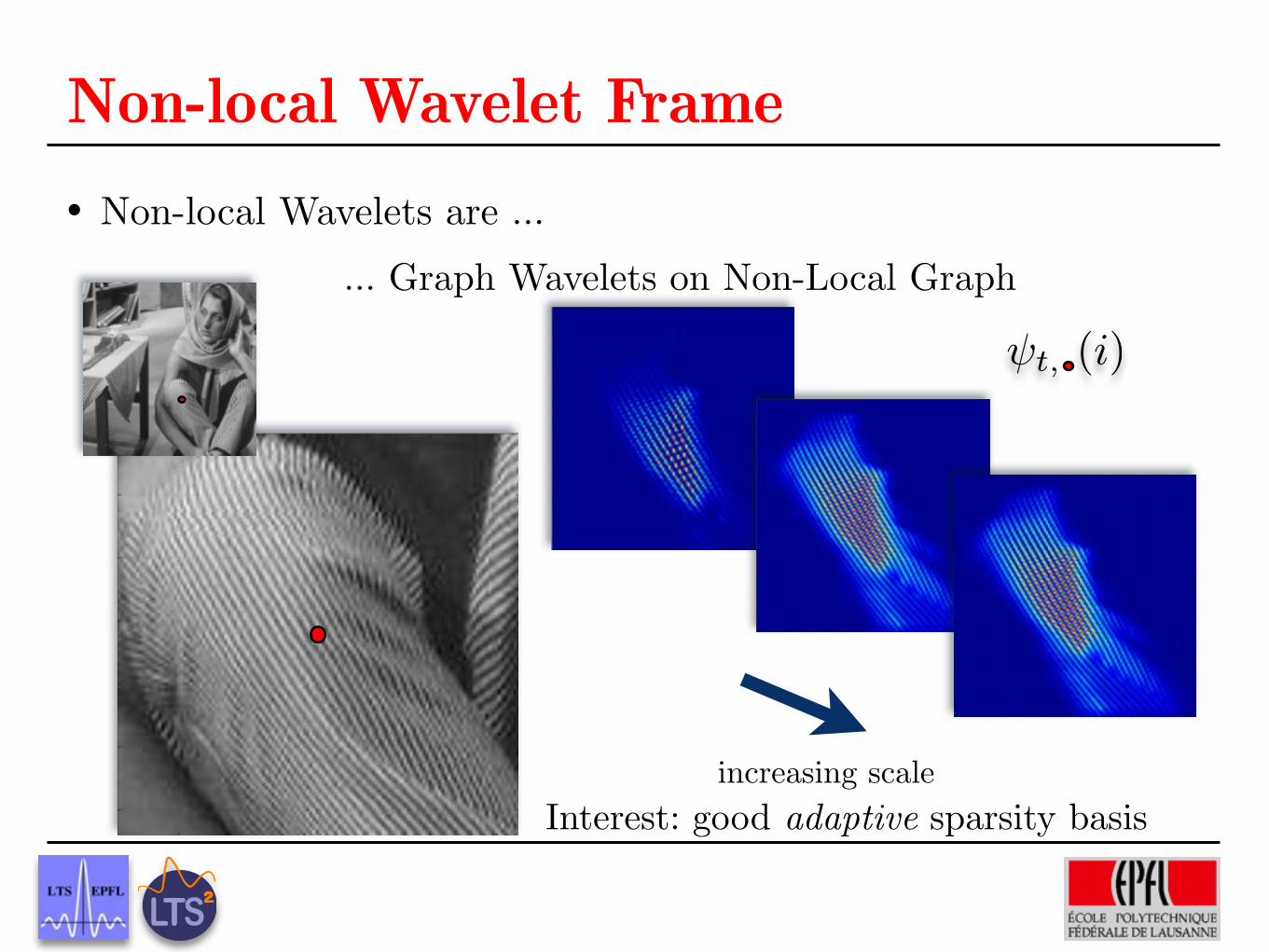
Non-local Wavelet Frame Non-local Wavelets are ...
... Graph Wavelets on Non-Local Graph
increasing scale
t, (i)
Interest: good adaptive sparsity basis
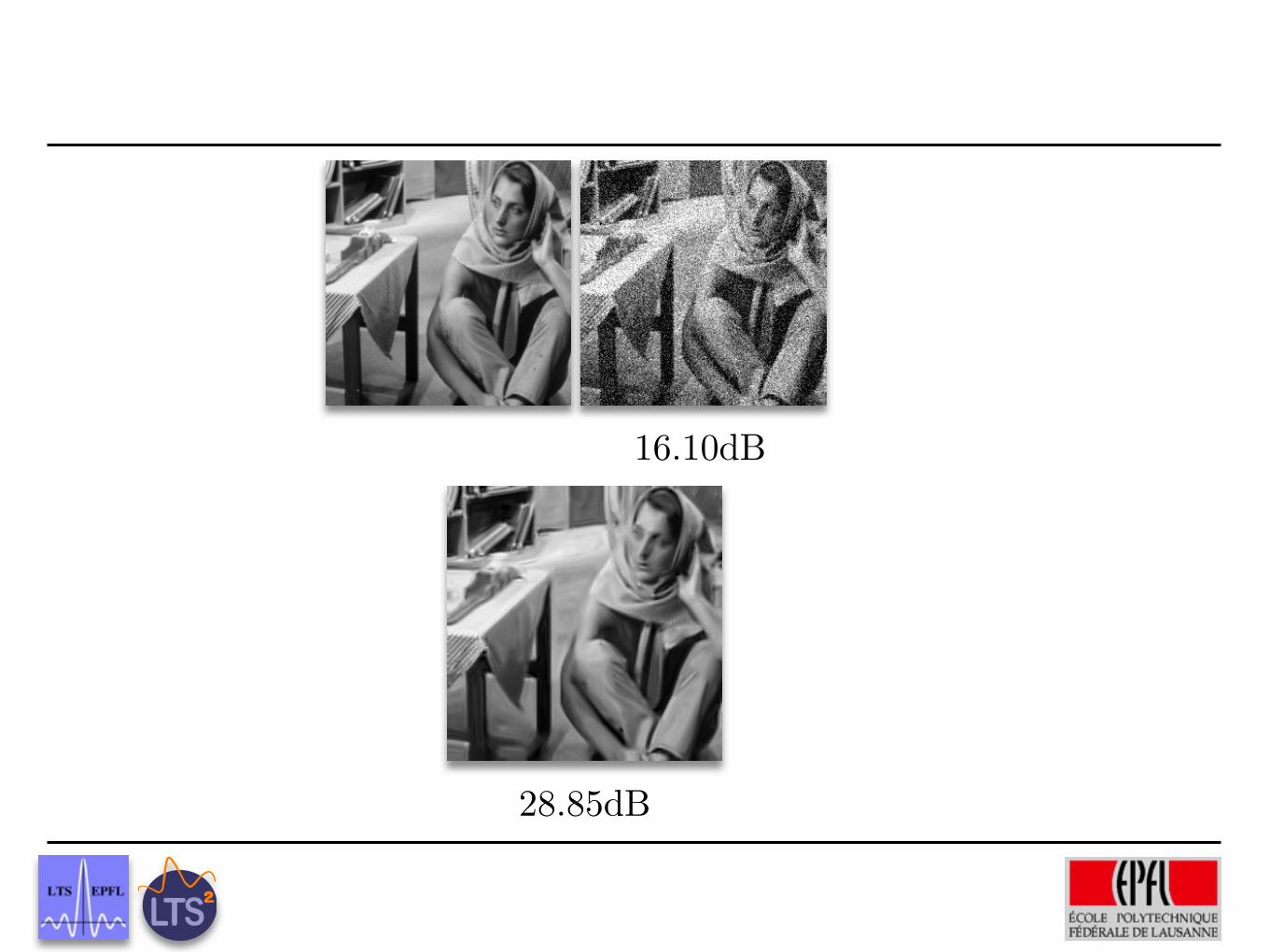
16.10dB
28.85dB
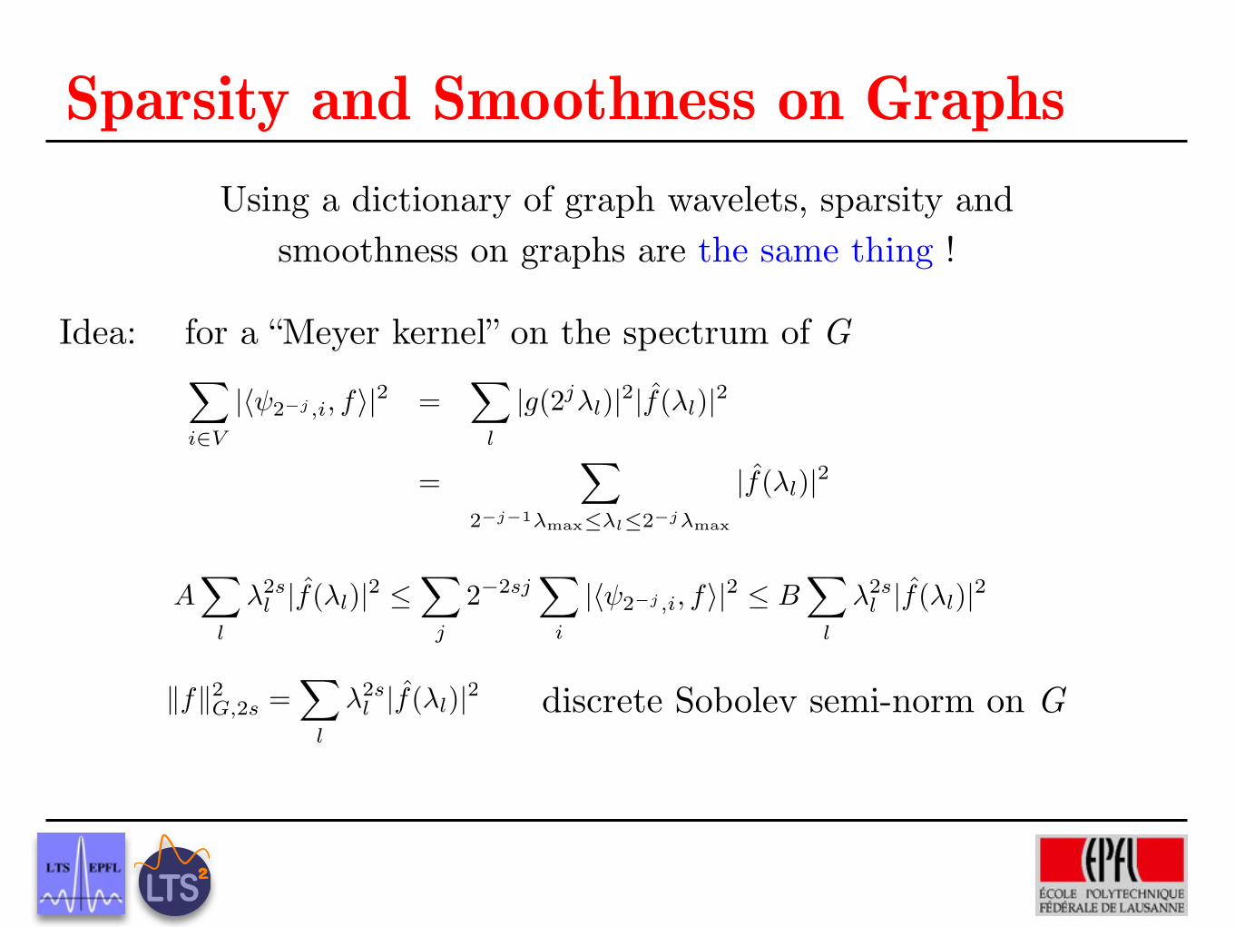
Sparsity and Smoothness on GraphsUsing a dictionary of graph wavelets, sparsity and
smoothness on graphs are the same thing !
Sparsity and Smoothness on GraphsUsing a dictionary of graph wavelets, sparsity and
smoothness on graphs are the same thing !
X
i2V
|h 2�j ,i, fi|2 =X
l
|g(2j�l)|2|f(�l)|2
=X
2�j�1�max
�l2�j�max
|f(�l)|2
AX
l
�2sl |f(�l)|2
X
j
2�2sjX
i
|h 2�j ,i, fi|2 BX
l
�2sl |f(�l)|2
kfk2G,2s =
X
l
�2sl |f(�l)|2
Idea: for a “Meyer kernel” on the spectrum of G
discrete Sobolev semi-norm on G
−98 −96 −94 −92 −90 −8844
46
48
−98 −96 −94 −92 −90 −8844
46
48
−98 −96 −94 −92 −90 −8844
46
48
−98 −96 −94 −92 −90 −8844
46
48
−98 −96 −94 −92 −90 −8844
46
48
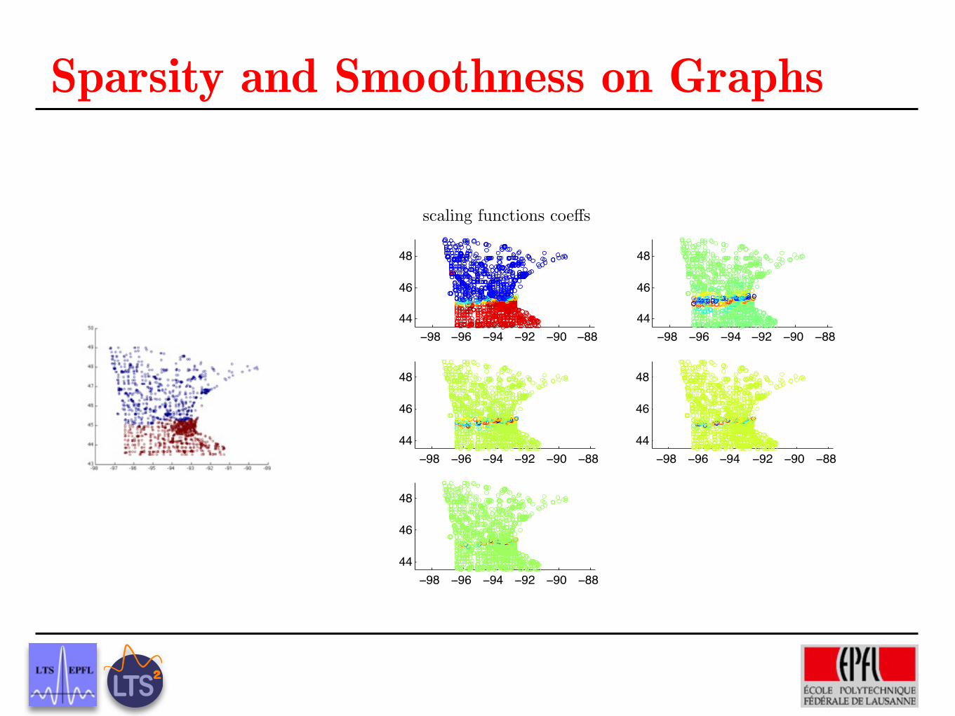
Sparsity and Smoothness on Graphs
scaling functions coeffs
arg min�ky �M�X�k2
2 + ↵k�k1
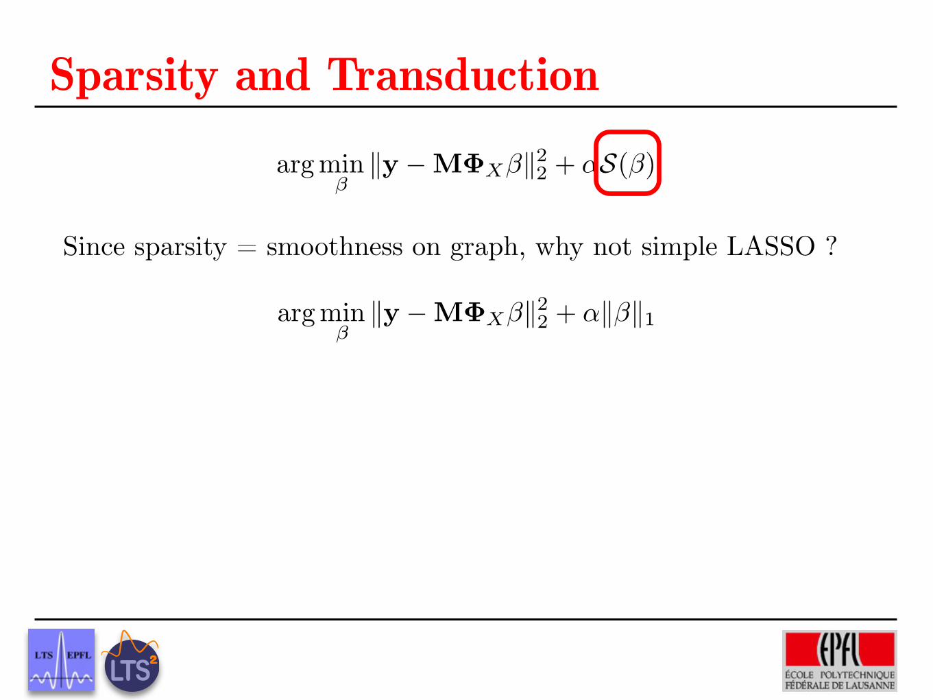
Sparsity and Transduction
Since sparsity = smoothness on graph, why not simple LASSO ?
arg min�ky �M�X�k2
2 + ↵S(�)
arg min�ky �M�X�k2
2 + ↵k�k1
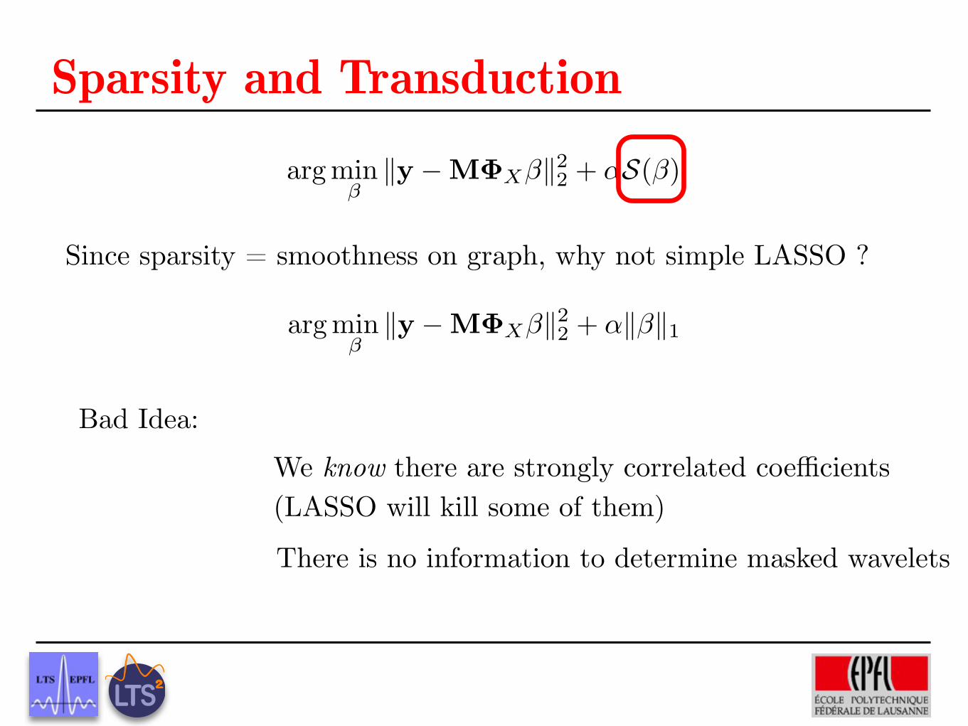
Sparsity and Transduction
Since sparsity = smoothness on graph, why not simple LASSO ?
arg min�ky �M�X�k2
2 + ↵S(�)
Bad Idea:We know there are strongly correlated coefficients (LASSO will kill some of them)
There is no information to determine masked wavelets
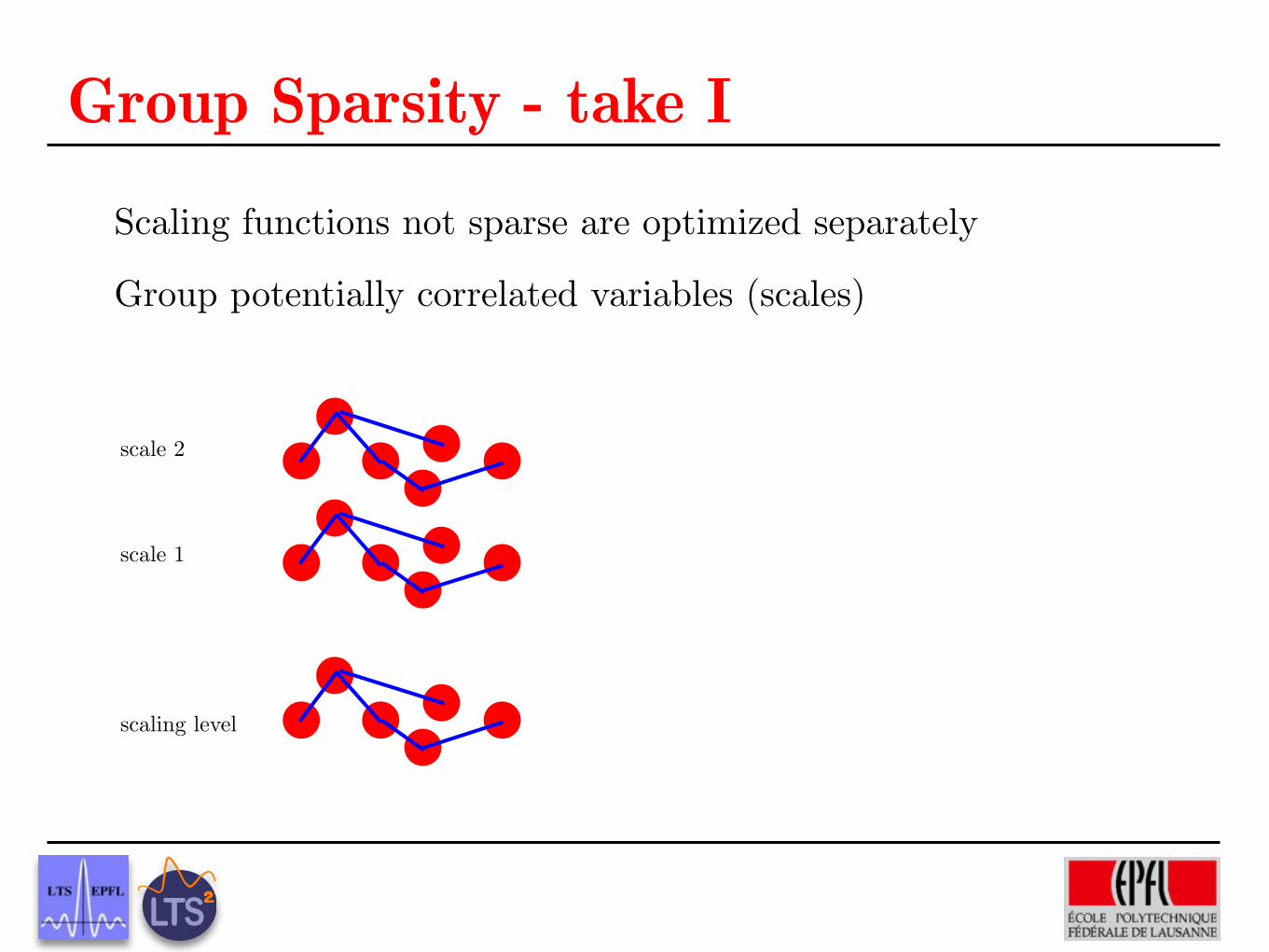
scaling level
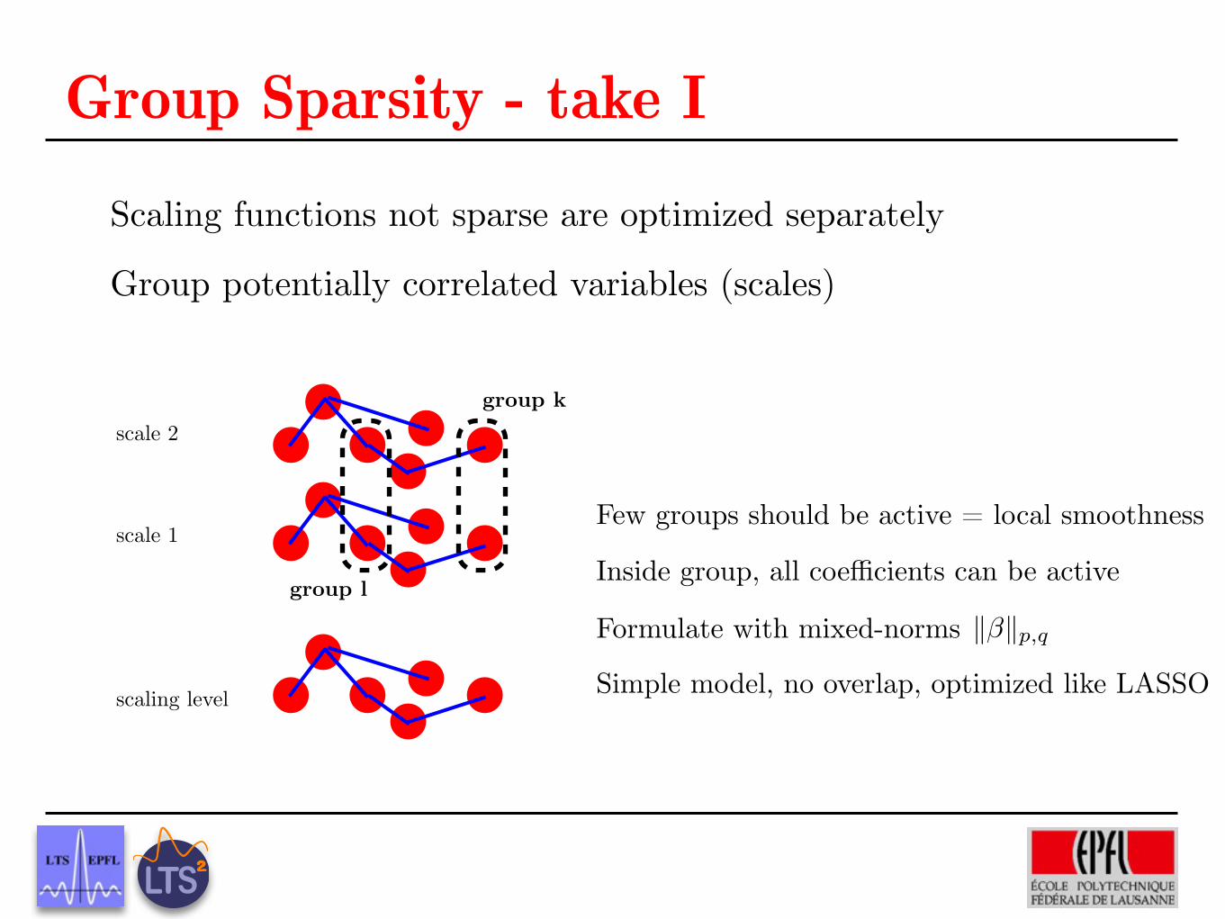
Group Sparsity - take IScaling functions not sparse are optimized separately
Group potentially correlated variables (scales)
scale 1
scale 2

scaling level
Group Sparsity - take IScaling functions not sparse are optimized separately
Group potentially correlated variables (scales)
scale 1
scale 2
group l
scaling level
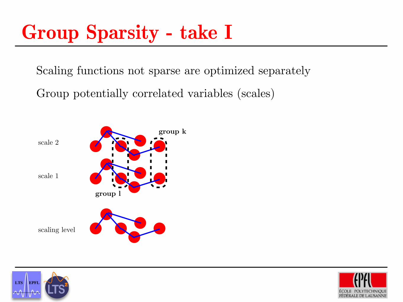
Group Sparsity - take IScaling functions not sparse are optimized separately
Group potentially correlated variables (scales)
scale 1
scale 2group k
group l
scaling level
Group Sparsity - take IScaling functions not sparse are optimized separately
Group potentially correlated variables (scales)
scale 1
scale 2group k
group l
Few groups should be active = local smoothness
Inside group, all coefficients can be active
Simple model, no overlap, optimized like LASSO
Formulate with mixed-norms k�kp,q
Preliminary Results
Ground truth
Wavelets on trees, graphs and high dimensional data
For a regression problem, our estimator for f is
f(x) =!
!,k,j
a!,k,j !!,k,j(x) (12)
whereas for binary classification we output sign(f).
Note that conditional on all subfolders of X!k having
at least one labeled point, a!,k,j is unbiased, E[a!,k,j ] =a!,k,j . For small folders there is a non-negligible prob-ability of having empty subfolders, so overall a!,k,j isbiased. However, by Theorem 1, for smooth functionsthese coe!cients are exponentially small in ". Thefollowing theorem quantifies the expected L2 error ofboth the estimate a!,k,j , and the function estimate f .Its proof is in the supplementary material.
Theorem 4 Let f be (C,#) Holder, and define C1 =C2"+1. Assume that the labeled samples si ! S " Xwere randomly chosen from the uniform distributionon X with replacement. Let f be the estimator (12)with coe!cients estimated via Eq. (11). Up to o(1/|S|)terms, the mean squared error of coe!cient estimatesis bounded by
E[a!,k,j # a!,k,j ]2 ! 1
|S|C2
1B2!
#(X"k)
2!
1!e!|S|B#(X"k)
(13)
+ 1B e!|S|B#(X"
k) · a2!,k,j
The resulting overall MSE is bounded by
E $f # f$2 = 1N
!
i
(f(xi)# f(xi))2
% C21B
2!
|S|
!
!,k,j
B2"(!!1)
1# e!|S|B" (14)
+ 22!+1C21
B
!
!,k,j
e!|S|B"
(B2"+1
)!!1
The first term in (13) is the estimation error whereasthe second term is the approximation error, e.g. thebias-variance decomposition. For su!ciently largefolders, with |S|B$(X!
k) & 1, the estimation error de-cays with the number of labeled points as |S|!1, and issmaller for smoother functions (larger #). The approx-imation error, due to folders empty of labeled points,decays exponentially with |S| and with folder size.
The values B and B can be easily extracted from agiven tree. Theorem 4 thus provides a non-parametricrisk analysis that depends on a single parameter, theassumed smoothness class # of the target function.
5. Numerical Results
We present preliminary numerical results of our SSLscheme on several datasets. More results and Matlab
0 20 40 60 80 1000
5
10
15
20
25
30
# of labeled points (out of 1500)
Test
Err
or
(%)
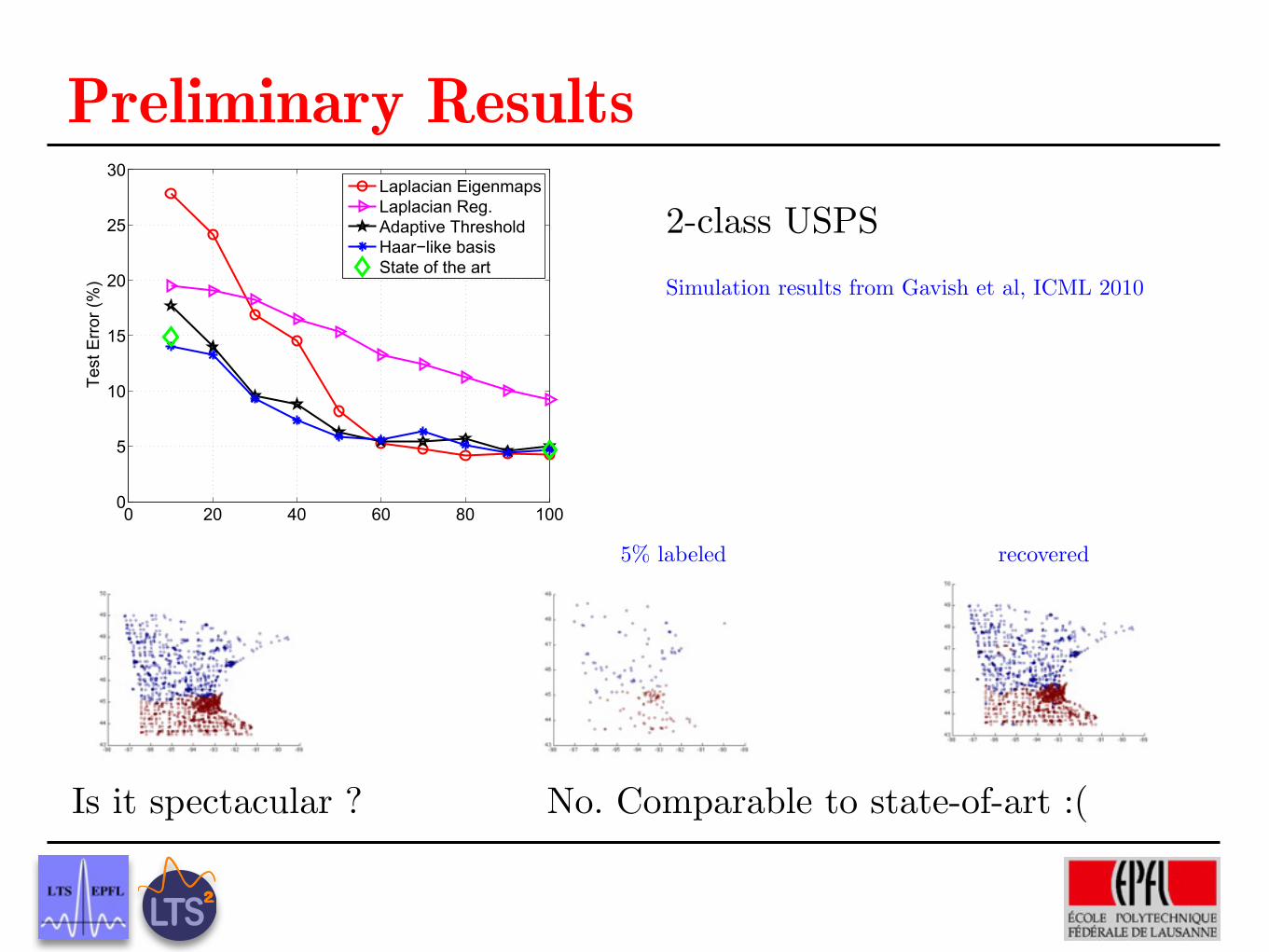
Laplacian EigenmapsLaplacian Reg.Adaptive ThresholdHaar!like basisState of the art
Figure 2. Results on the USPS benchmark.
code appear in supplementary material. We focus ontwo well-known handwritten digit data sets, MNISTand USPS. These are natural choices due to the inher-ent multiscale structures present in handwritten digits.
Given a dataset X of N digits, of which only a smallsubset S is labeled, we first use all samples inX to con-struct an a!nity matrix Wi,j described below. A treeis constructed as follows: At the finest level, " = L,we have N singleton folders: XL
i = {xi}. Each coarselevel is constructed from a finer level as follows: Ran-dom (centroid) points are selected s.t. no two are con-nected by an edge of weight larger than a ”radius”parameter. This yields a partition of the current levelaccording to the nearest centroid. The partition el-ements constitute the points of the coarser level. Acoarse a!nity matrix is constructed, where the edgeweight between two partition elements C and D is"
i"C,j"D W 2ij where W is the a!nity matrix of the
finer level graph. The motivation for squaring thea!nities at each new coarse level is to capture struc-tures at di"erent scales. As the choice of centroidsis (pseudo) random, so is the resulting partition tree.With the partition tree at hand, we construct a Haar-like basis induced by the tree and estimate the co-e!cients of the target label function as described inSection 4.
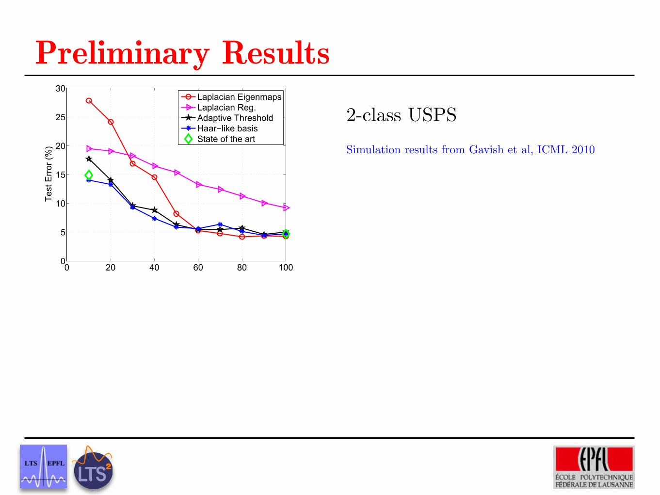
We compare our method to Laplacian Eigenmaps(Belkin & Niyogi, 2003), with |S|/5 eigenfunctions, assuggested by the authors, and to the Laplacian Reg-ularization approach of (Zhu et al., 2003). For thelatter, we also consider an adaptive threshold for clas-sification (sign(y > qth)), with qth chosen such thatthe proportion of test labeled points of each class isequal to its value in the training set2.
2Note that this method is di!erent from the class massnormalization approach of (Zhu et al., 2003).
Simulation results from Gavish et al, ICML 2010
2-class USPS
Preliminary Results
Ground truth
Wavelets on trees, graphs and high dimensional data
For a regression problem, our estimator for f is
f(x) =!
!,k,j
a!,k,j !!,k,j(x) (12)
whereas for binary classification we output sign(f).
Note that conditional on all subfolders of X!k having
at least one labeled point, a!,k,j is unbiased, E[a!,k,j ] =a!,k,j . For small folders there is a non-negligible prob-ability of having empty subfolders, so overall a!,k,j isbiased. However, by Theorem 1, for smooth functionsthese coe!cients are exponentially small in ". Thefollowing theorem quantifies the expected L2 error ofboth the estimate a!,k,j , and the function estimate f .Its proof is in the supplementary material.
Theorem 4 Let f be (C,#) Holder, and define C1 =C2"+1. Assume that the labeled samples si ! S " Xwere randomly chosen from the uniform distributionon X with replacement. Let f be the estimator (12)with coe!cients estimated via Eq. (11). Up to o(1/|S|)terms, the mean squared error of coe!cient estimatesis bounded by
E[a!,k,j # a!,k,j ]2 ! 1
|S|C2
1B2!
#(X"k)
2!
1!e!|S|B#(X"k)
(13)
+ 1B e!|S|B#(X"
k) · a2!,k,j
The resulting overall MSE is bounded by
E $f # f$2 = 1N
!
i
(f(xi)# f(xi))2
% C21B
2!
|S|
!
!,k,j
B2"(!!1)
1# e!|S|B" (14)
+ 22!+1C21
B
!
!,k,j
e!|S|B"
(B2"+1
)!!1
The first term in (13) is the estimation error whereasthe second term is the approximation error, e.g. thebias-variance decomposition. For su!ciently largefolders, with |S|B$(X!
k) & 1, the estimation error de-cays with the number of labeled points as |S|!1, and issmaller for smoother functions (larger #). The approx-imation error, due to folders empty of labeled points,decays exponentially with |S| and with folder size.
The values B and B can be easily extracted from agiven tree. Theorem 4 thus provides a non-parametricrisk analysis that depends on a single parameter, theassumed smoothness class # of the target function.
5. Numerical Results
We present preliminary numerical results of our SSLscheme on several datasets. More results and Matlab
0 20 40 60 80 1000
5
10
15
20
25
30
# of labeled points (out of 1500)
Test
Err
or
(%)
Laplacian EigenmapsLaplacian Reg.Adaptive ThresholdHaar!like basisState of the art
Figure 2. Results on the USPS benchmark.
code appear in supplementary material. We focus ontwo well-known handwritten digit data sets, MNISTand USPS. These are natural choices due to the inher-ent multiscale structures present in handwritten digits.
Given a dataset X of N digits, of which only a smallsubset S is labeled, we first use all samples inX to con-struct an a!nity matrix Wi,j described below. A treeis constructed as follows: At the finest level, " = L,we have N singleton folders: XL
i = {xi}. Each coarselevel is constructed from a finer level as follows: Ran-dom (centroid) points are selected s.t. no two are con-nected by an edge of weight larger than a ”radius”parameter. This yields a partition of the current levelaccording to the nearest centroid. The partition el-ements constitute the points of the coarser level. Acoarse a!nity matrix is constructed, where the edgeweight between two partition elements C and D is"
i"C,j"D W 2ij where W is the a!nity matrix of the
finer level graph. The motivation for squaring thea!nities at each new coarse level is to capture struc-tures at di"erent scales. As the choice of centroidsis (pseudo) random, so is the resulting partition tree.With the partition tree at hand, we construct a Haar-like basis induced by the tree and estimate the co-e!cients of the target label function as described inSection 4.
We compare our method to Laplacian Eigenmaps(Belkin & Niyogi, 2003), with |S|/5 eigenfunctions, assuggested by the authors, and to the Laplacian Reg-ularization approach of (Zhu et al., 2003). For thelatter, we also consider an adaptive threshold for clas-sification (sign(y > qth)), with qth chosen such thatthe proportion of test labeled points of each class isequal to its value in the training set2.
2Note that this method is di!erent from the class massnormalization approach of (Zhu et al., 2003).
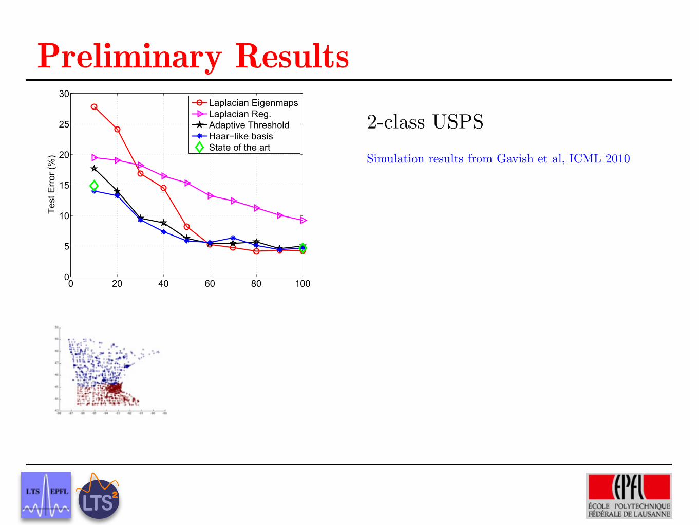
Simulation results from Gavish et al, ICML 2010
2-class USPS
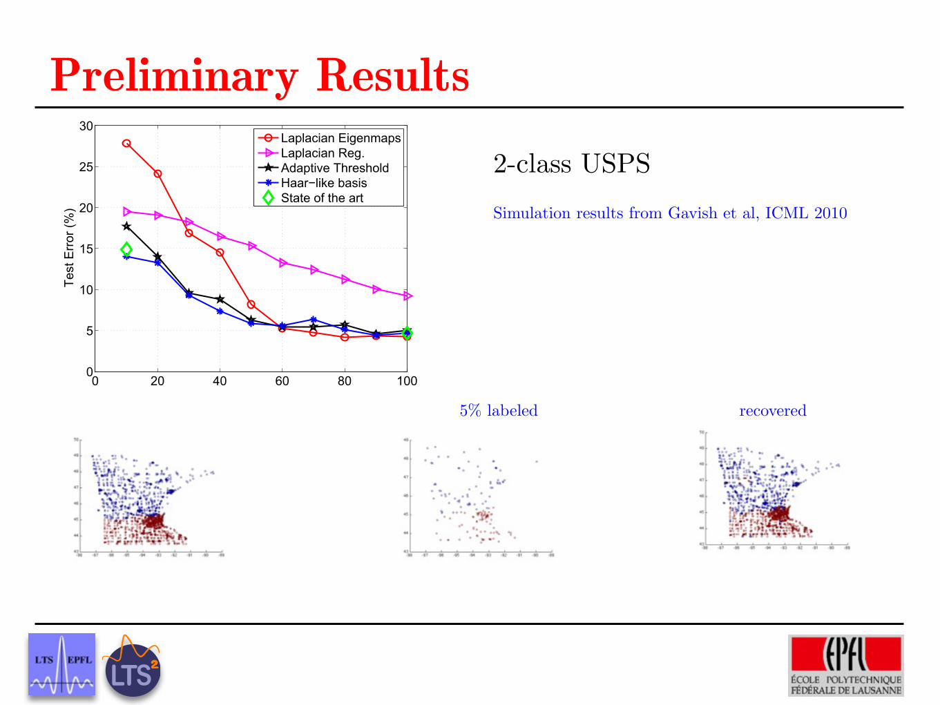
Preliminary Results
Ground truth
5% labeled recovered
Wavelets on trees, graphs and high dimensional data
For a regression problem, our estimator for f is
f(x) =!
!,k,j
a!,k,j !!,k,j(x) (12)
whereas for binary classification we output sign(f).
Note that conditional on all subfolders of X!k having
at least one labeled point, a!,k,j is unbiased, E[a!,k,j ] =a!,k,j . For small folders there is a non-negligible prob-ability of having empty subfolders, so overall a!,k,j isbiased. However, by Theorem 1, for smooth functionsthese coe!cients are exponentially small in ". Thefollowing theorem quantifies the expected L2 error ofboth the estimate a!,k,j , and the function estimate f .Its proof is in the supplementary material.
Theorem 4 Let f be (C,#) Holder, and define C1 =C2"+1. Assume that the labeled samples si ! S " Xwere randomly chosen from the uniform distributionon X with replacement. Let f be the estimator (12)with coe!cients estimated via Eq. (11). Up to o(1/|S|)terms, the mean squared error of coe!cient estimatesis bounded by
E[a!,k,j # a!,k,j ]2 ! 1
|S|C2
1B2!
#(X"k)
2!
1!e!|S|B#(X"k)
(13)
+ 1B e!|S|B#(X"
k) · a2!,k,j
The resulting overall MSE is bounded by
E $f # f$2 = 1N
!
i
(f(xi)# f(xi))2
% C21B
2!
|S|
!
!,k,j
B2"(!!1)
1# e!|S|B" (14)
+ 22!+1C21
B
!
!,k,j
e!|S|B"
(B2"+1
)!!1
The first term in (13) is the estimation error whereasthe second term is the approximation error, e.g. thebias-variance decomposition. For su!ciently largefolders, with |S|B$(X!
k) & 1, the estimation error de-cays with the number of labeled points as |S|!1, and issmaller for smoother functions (larger #). The approx-imation error, due to folders empty of labeled points,decays exponentially with |S| and with folder size.
The values B and B can be easily extracted from agiven tree. Theorem 4 thus provides a non-parametricrisk analysis that depends on a single parameter, theassumed smoothness class # of the target function.
5. Numerical Results
We present preliminary numerical results of our SSLscheme on several datasets. More results and Matlab
0 20 40 60 80 1000
5
10
15
20
25
30
# of labeled points (out of 1500)
Test
Err
or
(%)
Laplacian EigenmapsLaplacian Reg.Adaptive ThresholdHaar!like basisState of the art
Figure 2. Results on the USPS benchmark.
code appear in supplementary material. We focus ontwo well-known handwritten digit data sets, MNISTand USPS. These are natural choices due to the inher-ent multiscale structures present in handwritten digits.
Given a dataset X of N digits, of which only a smallsubset S is labeled, we first use all samples inX to con-struct an a!nity matrix Wi,j described below. A treeis constructed as follows: At the finest level, " = L,we have N singleton folders: XL
i = {xi}. Each coarselevel is constructed from a finer level as follows: Ran-dom (centroid) points are selected s.t. no two are con-nected by an edge of weight larger than a ”radius”parameter. This yields a partition of the current levelaccording to the nearest centroid. The partition el-ements constitute the points of the coarser level. Acoarse a!nity matrix is constructed, where the edgeweight between two partition elements C and D is"
i"C,j"D W 2ij where W is the a!nity matrix of the
finer level graph. The motivation for squaring thea!nities at each new coarse level is to capture struc-tures at di"erent scales. As the choice of centroidsis (pseudo) random, so is the resulting partition tree.With the partition tree at hand, we construct a Haar-like basis induced by the tree and estimate the co-e!cients of the target label function as described inSection 4.
We compare our method to Laplacian Eigenmaps(Belkin & Niyogi, 2003), with |S|/5 eigenfunctions, assuggested by the authors, and to the Laplacian Reg-ularization approach of (Zhu et al., 2003). For thelatter, we also consider an adaptive threshold for clas-sification (sign(y > qth)), with qth chosen such thatthe proportion of test labeled points of each class isequal to its value in the training set2.
2Note that this method is di!erent from the class massnormalization approach of (Zhu et al., 2003).
Simulation results from Gavish et al, ICML 2010
2-class USPS
Preliminary Results
Ground truth
5% labeled recovered
Is it spectacular ? No. Comparable to state-of-art :(
Wavelets on trees, graphs and high dimensional data
For a regression problem, our estimator for f is
f(x) =!
!,k,j
a!,k,j !!,k,j(x) (12)
whereas for binary classification we output sign(f).
Note that conditional on all subfolders of X!k having
at least one labeled point, a!,k,j is unbiased, E[a!,k,j ] =a!,k,j . For small folders there is a non-negligible prob-ability of having empty subfolders, so overall a!,k,j isbiased. However, by Theorem 1, for smooth functionsthese coe!cients are exponentially small in ". Thefollowing theorem quantifies the expected L2 error ofboth the estimate a!,k,j , and the function estimate f .Its proof is in the supplementary material.
Theorem 4 Let f be (C,#) Holder, and define C1 =C2"+1. Assume that the labeled samples si ! S " Xwere randomly chosen from the uniform distributionon X with replacement. Let f be the estimator (12)with coe!cients estimated via Eq. (11). Up to o(1/|S|)terms, the mean squared error of coe!cient estimatesis bounded by
E[a!,k,j # a!,k,j ]2 ! 1
|S|C2
1B2!
#(X"k)
2!
1!e!|S|B#(X"k)
(13)
+ 1B e!|S|B#(X"
k) · a2!,k,j
The resulting overall MSE is bounded by
E $f # f$2 = 1N
!
i
(f(xi)# f(xi))2
% C21B
2!
|S|
!
!,k,j
B2"(!!1)
1# e!|S|B" (14)
+ 22!+1C21
B
!
!,k,j
e!|S|B"
(B2"+1
)!!1
The first term in (13) is the estimation error whereasthe second term is the approximation error, e.g. thebias-variance decomposition. For su!ciently largefolders, with |S|B$(X!
k) & 1, the estimation error de-cays with the number of labeled points as |S|!1, and issmaller for smoother functions (larger #). The approx-imation error, due to folders empty of labeled points,decays exponentially with |S| and with folder size.
The values B and B can be easily extracted from agiven tree. Theorem 4 thus provides a non-parametricrisk analysis that depends on a single parameter, theassumed smoothness class # of the target function.
5. Numerical Results
We present preliminary numerical results of our SSLscheme on several datasets. More results and Matlab
0 20 40 60 80 1000
5
10
15
20
25
30
# of labeled points (out of 1500)
Test
Err
or
(%)
Laplacian EigenmapsLaplacian Reg.Adaptive ThresholdHaar!like basisState of the art
Figure 2. Results on the USPS benchmark.
code appear in supplementary material. We focus ontwo well-known handwritten digit data sets, MNISTand USPS. These are natural choices due to the inher-ent multiscale structures present in handwritten digits.
Given a dataset X of N digits, of which only a smallsubset S is labeled, we first use all samples inX to con-struct an a!nity matrix Wi,j described below. A treeis constructed as follows: At the finest level, " = L,we have N singleton folders: XL
i = {xi}. Each coarselevel is constructed from a finer level as follows: Ran-dom (centroid) points are selected s.t. no two are con-nected by an edge of weight larger than a ”radius”parameter. This yields a partition of the current levelaccording to the nearest centroid. The partition el-ements constitute the points of the coarser level. Acoarse a!nity matrix is constructed, where the edgeweight between two partition elements C and D is"
i"C,j"D W 2ij where W is the a!nity matrix of the
finer level graph. The motivation for squaring thea!nities at each new coarse level is to capture struc-tures at di"erent scales. As the choice of centroidsis (pseudo) random, so is the resulting partition tree.With the partition tree at hand, we construct a Haar-like basis induced by the tree and estimate the co-e!cients of the target label function as described inSection 4.
We compare our method to Laplacian Eigenmaps(Belkin & Niyogi, 2003), with |S|/5 eigenfunctions, assuggested by the authors, and to the Laplacian Reg-ularization approach of (Zhu et al., 2003). For thelatter, we also consider an adaptive threshold for clas-sification (sign(y > qth)), with qth chosen such thatthe proportion of test labeled points of each class isequal to its value in the training set2.
2Note that this method is di!erent from the class massnormalization approach of (Zhu et al., 2003).
Simulation results from Gavish et al, ICML 2010
2-class USPS

Group Sparsity - take II (outlook)Group definition too restrictive
No “spatial” (neighborhood) information
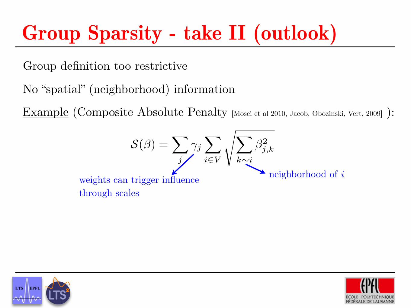
Group Sparsity - take II (outlook)Group definition too restrictive
No “spatial” (neighborhood) information
S(�) =X
j
�j
X
i2V
sX
k⇠i
�2j,k
neighborhood of i
Example (Composite Absolute Penalty [Mosci et al 2010, Jacob, Obozinski, Vert, 2009] ):
weights can trigger influence through scales
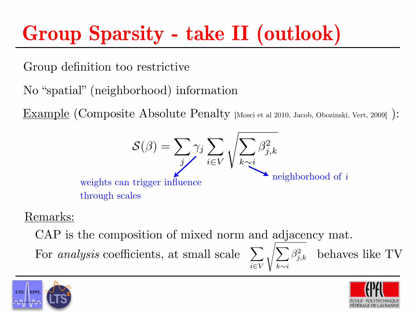
Group Sparsity - take II (outlook)Group definition too restrictive
No “spatial” (neighborhood) information
S(�) =X
j
�j
X
i2V
sX
k⇠i
�2j,k
neighborhood of i
Example (Composite Absolute Penalty [Mosci et al 2010, Jacob, Obozinski, Vert, 2009] ):
weights can trigger influence through scales
X
i2V
sX
k⇠i
�2j,k
Remarks:CAP is the composition of mixed norm and adjacency mat.For analysis coefficients, at small scale behaves like TV
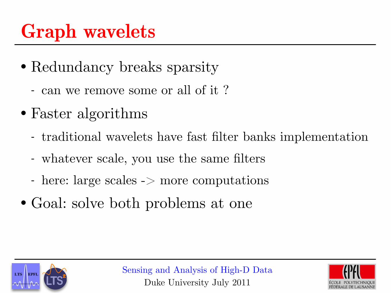
Sensing and Analysis of High-D DataDuke University July 2011
Graph wavelets Redundancy breaks sparsity- can we remove some or all of it ?
Faster algorithms- traditional wavelets have fast filter banks implementation- whatever scale, you use the same filters- here: large scales -> more computations
Goal: solve both problems at one
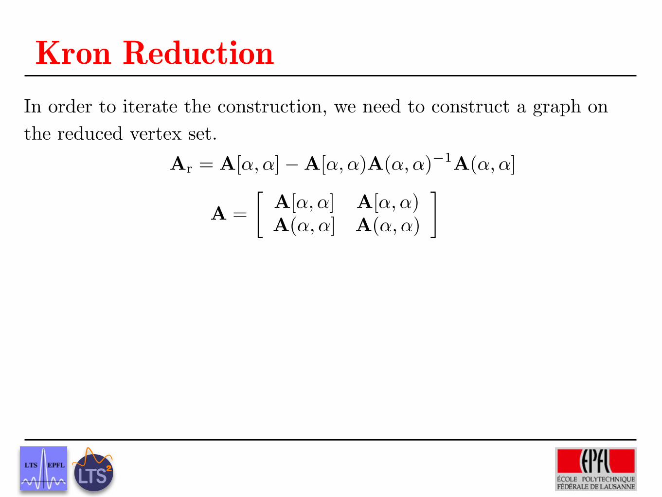
Ar = A[↵,↵]�A[↵,↵)A(↵,↵)�1A(↵,↵]
A =
A[↵,↵] A[↵,↵)A(↵,↵] A(↵,↵)
�
Kron ReductionIn order to iterate the construction, we need to construct a graph on the reduced vertex set.
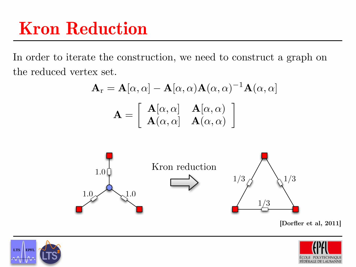
Ar = A[↵,↵]�A[↵,↵)A(↵,↵)�1A(↵,↵]
A =
A[↵,↵] A[↵,↵)A(↵,↵] A(↵,↵)
�
Kron ReductionIn order to iterate the construction, we need to construct a graph on the reduced vertex set.
2 F. Dorfler and F. Bullo
is the loopy Laplacian matrix. In various applications of circuit theory and relateddisciplines it is desirable to obtain a lower dimensional electrically-equivalent networkfrom the viewpoint of certain boundary nodes (or terminals) � � {1, . . . , n}, |�| ⌅ 2.If ⇥ = {1, . . . , n}\� denotes the set of interior nodes, then, after appropriately labelingthe nodes, the current-balance equations can be partitioned as
�I�I⇥
⇥=
�Q�� Q�⇥
Q⇥� Q⇥⇥
⇥ �V�
V⇥
⇥. (1.1)
Gaussian elimination of the interior voltages V⇥ in equations (1.1) gives an electrically-equivalent reduced network with |�| nodes obeying the reduced current-balances
I� +QacI⇥ = QredV� , (1.2)
where the reduced conductance matrixQred ⇧ R|�|⇥|�| is again a loopy Laplacian givenby the Schur complement of Q with respect to the interior nodes ⇥, that is, Qred =Q���Q�⇥Q
�1⇥⇥Q⇥�. The accompanying matrix Qac = �Q�⇥Q
�1⇥⇥ ⇧ R|�|⇥(n�|�|) maps
internal currents to boundary currents in the reduced network. In case that I⇥ is thevector of zeros, the (i, j)-element of Qred is the current at boundary node i due to aunit potential at boundary node j and a zero potential at all other boundary nodes.From here the reduced network can be further analyzed as an |�|-port with currentinjections I� +QacI⇥ and transfer conductance matrix Qred.
This reduction of an electrical network via a Schur complement of the associatedconductance matrix is known as Kron reduction due to the seminal work of GabrielKron [37], who identified fundamental interconnections among physics, linear algebra,and graph theory [33, 38]. The Kron reduction of a simple tree-like network with-out current injections or shunt conductances is illustrated in Figure 1.1, an examplefamiliar to every engineering student as the Y �� transformation.
8
8
8
30
1.0 1.0
1.0Kron reduction
8
8
8
1/3
1/31/3
Fig. 1.1. Kron reduction of a star-like electrical circuit with three boundary nodes ⇥�, oneinterior node •⇥ , and with unit conductances resulting in a reduced triangular reduced circuit.
Literature Review. The Kron reduction of networks is ubiquitous in circuittheory and related applications in order to obtain lower dimensional electrically-equivalent circuits. It appears for instance in the behavior, synthesis, and analysis ofresistive circuits [56, 60, 59], particularly in the context of large-scale integration chips[48, 53, 1]. When applied to the impedance matrix of a circuit rather than the admit-tance matrix, Kron reduction is also referred to as the “shortage operator” [2, 3, 35].Kron reduction is a standard tool in the power systems community to obtain station-ary and dynamically-equivalent reduced models for power flow studies [58, 10, 61], orin the reduction of di⇥erential-algebraic power network and RLC circuit models tolower dimensional purely dynamic models [45, 52, 5, 18, 20]. A recent application ofKron reduction is monitoring in smart power grids [17] via synchronized phasor mea-surement units. Kron reduction is also crucial for reduced order modeling, analysis,
[Dorfler et al, 2011]
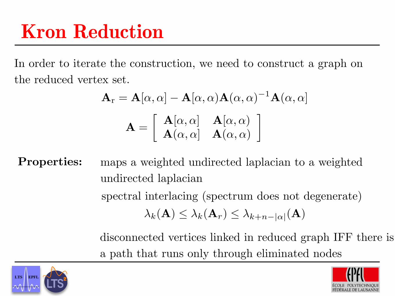
Ar = A[↵,↵]�A[↵,↵)A(↵,↵)�1A(↵,↵]
A =
A[↵,↵] A[↵,↵)A(↵,↵] A(↵,↵)
�
�k(A) �k(Ar) �k+n�|↵|(A)
Kron Reduction
Properties:
In order to iterate the construction, we need to construct a graph on the reduced vertex set.
maps a weighted undirected laplacian to a weighted undirected laplacianspectral interlacing (spectrum does not degenerate)
disconnected vertices linked in reduced graph IFF there is a path that runs only through eliminated nodes
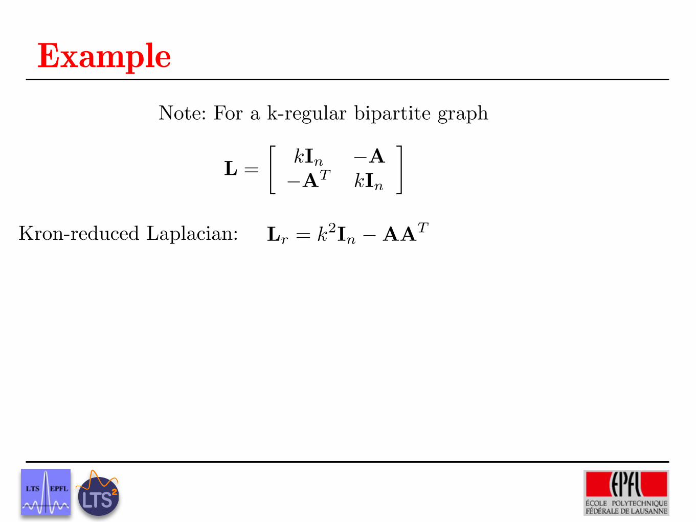
L =
kIn �A�AT kIn
�
Lr = k2In �AAT
ExampleNote: For a k-regular bipartite graph
Kron-reduced Laplacian:
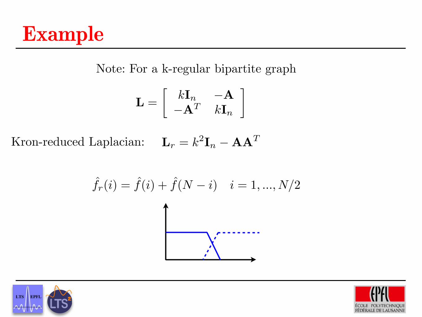
L =
kIn �A�AT kIn
�
Lr = k2In �AAT
ExampleNote: For a k-regular bipartite graph
Kron-reduced Laplacian:
fr(i) = f(i) + f(N � i) i = 1, ..., N/2
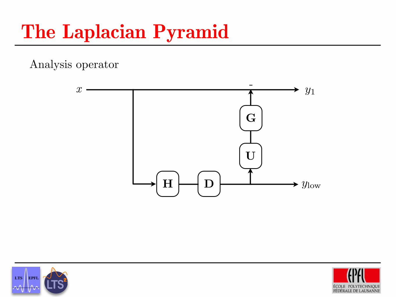
The Laplacian PyramidAnalysis operator
y1
ylow
H D
U
G
-x

The Laplacian PyramidAnalysis operator
y0
y1
H D U
G
-x
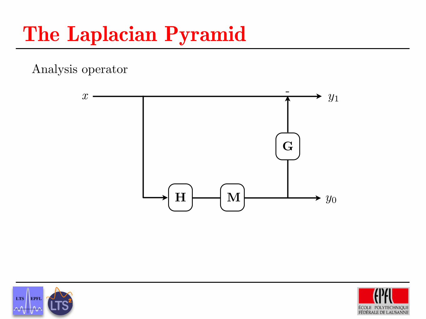
The Laplacian PyramidAnalysis operator
y0
y1
H M
G
-x
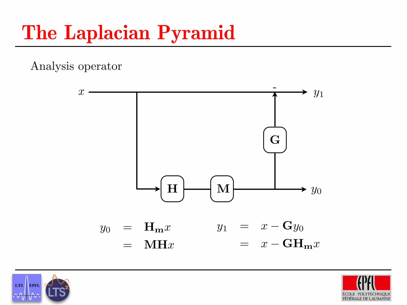
The Laplacian PyramidAnalysis operator
y0
y1
H M
G
-x
y0 = Hmx
= MHx
y1 = x�Gy0
= x�GHmx

The Laplacian PyramidAnalysis operator
y0
y1
H M
G
-x
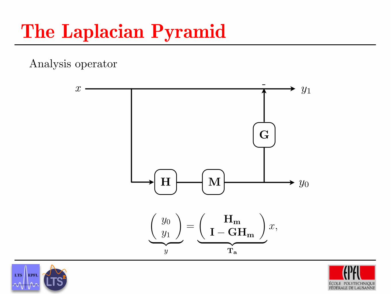
The Laplacian PyramidAnalysis operator
y0
y1
H M
G
-x
upsampling by masking operator M where M is a diagonal matrix with onesat on-diagonal entries correspond to the location of the selected vertices, andzeros elsewhere.
Then we will pass the output of the masking block through a second filterg in order to reconstruct the original function. Finally, the reconstructionerror is easily computed by taking di�erence of the original signal and theoutput of the second filter.
Consider an input graph-signal x ⇤ Rn. In our notation, y0 = Hmxdenotes the output of h-filtering followed by masking operator. This is theoutput of the lowpass channel in the LP framework.
y0 = Hmx
= MHx
= MVHVTx, (5.1)
where V = [v0|v1|...|vn�1] is the matrix of the eigenvectors of graph Lapla-cian L and H is a diagonal matrix with on-diagonal entries {h(�l)}n�1
l=0 ando�-diagonal entries equal to zero. Recall that the multiplier is the real-valuedfunction h : R+ ⇥ R+.
The output of the highpass channel is then given by y1 = x�Gy0 whichis equal to the reconstruction error.
y1 = x�Gx
= x�VGVTx, (5.2)
where V is defined earlier and G is a diagonal matrix with on-diagonal entries{g(�l)}n�1
l=0 and o�-diagonal entries equal to zero. Note that for the secondfilter we use the multiplier g : R+ ⇥ R+.
The analysis operator Ta is then defined in
�y0
y1
⇥
⇧ ⌅⇤ ⌃y
=
�Hm
I�GHm
⇥
⇧ ⌅⇤ ⌃Ta
x, (5.3)
where y0, y1 ⇤ Rn are the coarse and prediction error coe⇤cients respectively.Fig. 5.1 shows the analysis part of the graph Laplacian Pyramid.
30
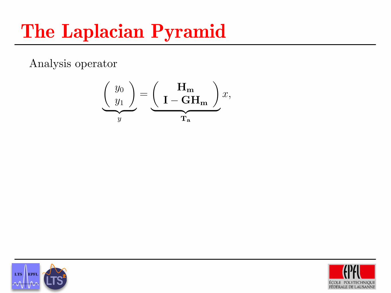
The Laplacian PyramidAnalysis operator
upsampling by masking operator M where M is a diagonal matrix with onesat on-diagonal entries correspond to the location of the selected vertices, andzeros elsewhere.
Then we will pass the output of the masking block through a second filterg in order to reconstruct the original function. Finally, the reconstructionerror is easily computed by taking di�erence of the original signal and theoutput of the second filter.
Consider an input graph-signal x ⇤ Rn. In our notation, y0 = Hmxdenotes the output of h-filtering followed by masking operator. This is theoutput of the lowpass channel in the LP framework.
y0 = Hmx
= MHx
= MVHVTx, (5.1)
where V = [v0|v1|...|vn�1] is the matrix of the eigenvectors of graph Lapla-cian L and H is a diagonal matrix with on-diagonal entries {h(�l)}n�1
l=0 ando�-diagonal entries equal to zero. Recall that the multiplier is the real-valuedfunction h : R+ ⇥ R+.
The output of the highpass channel is then given by y1 = x�Gy0 whichis equal to the reconstruction error.
y1 = x�Gx
= x�VGVTx, (5.2)
where V is defined earlier and G is a diagonal matrix with on-diagonal entries{g(�l)}n�1
l=0 and o�-diagonal entries equal to zero. Note that for the secondfilter we use the multiplier g : R+ ⇥ R+.
The analysis operator Ta is then defined in
�y0
y1
⇥
⇧ ⌅⇤ ⌃y
=
�Hm
I�GHm
⇥
⇧ ⌅⇤ ⌃Ta
x, (5.3)
where y0, y1 ⇤ Rn are the coarse and prediction error coe⇤cients respectively.Fig. 5.1 shows the analysis part of the graph Laplacian Pyramid.
30
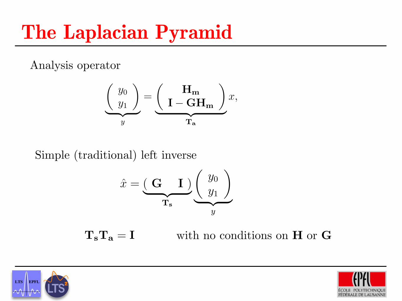
The Laplacian PyramidAnalysis operator
upsampling by masking operator M where M is a diagonal matrix with onesat on-diagonal entries correspond to the location of the selected vertices, andzeros elsewhere.
Then we will pass the output of the masking block through a second filterg in order to reconstruct the original function. Finally, the reconstructionerror is easily computed by taking di�erence of the original signal and theoutput of the second filter.
Consider an input graph-signal x ⇤ Rn. In our notation, y0 = Hmxdenotes the output of h-filtering followed by masking operator. This is theoutput of the lowpass channel in the LP framework.
y0 = Hmx
= MHx
= MVHVTx, (5.1)
where V = [v0|v1|...|vn�1] is the matrix of the eigenvectors of graph Lapla-cian L and H is a diagonal matrix with on-diagonal entries {h(�l)}n�1
l=0 ando�-diagonal entries equal to zero. Recall that the multiplier is the real-valuedfunction h : R+ ⇥ R+.
The output of the highpass channel is then given by y1 = x�Gy0 whichis equal to the reconstruction error.
y1 = x�Gx
= x�VGVTx, (5.2)
where V is defined earlier and G is a diagonal matrix with on-diagonal entries{g(�l)}n�1
l=0 and o�-diagonal entries equal to zero. Note that for the secondfilter we use the multiplier g : R+ ⇥ R+.
The analysis operator Ta is then defined in
�y0
y1
⇥
⇧ ⌅⇤ ⌃y
=
�Hm
I�GHm
⇥
⇧ ⌅⇤ ⌃Ta
x, (5.3)
where y0, y1 ⇤ Rn are the coarse and prediction error coe⇤cients respectively.Fig. 5.1 shows the analysis part of the graph Laplacian Pyramid.
30
TsTa = I
Simple (traditional) left inverse
Figure 5.1: Analysis scheme in graph Laplacian pyramid.
The usual inverse transform of the LP for reconstruction of the originalsignal is also given in
x = ( G I )⇧ ⌅⇤ ⌃Ts
�y0
y1
⇥
⇧ ⌅⇤ ⌃y
. (5.4)
First, we predict the original signal by filtering of the coarse version y0 andadd the reconstruction error y1 to recover the original signal x completely.Fig. 5.2 shows the usual inverse transform of the graph LP.
Figure 5.2: Usual synthesis scheme in graph Laplacian pyramid.
It is easy to check that TsTa = I for any Hm,G. In fact, it shows that LPcan be perfectly reconstructed with any pairs of filters Hm,G. Analogouslyto the classical Laplacian pyramid, since the graph LP is also a redundanttransform, an infinite number of left inverses are admitted as synthesis oper-ator. The most important one among those is the pseudo inverse
Ta† = (Ta
TTa)�1Ta
T . (5.5)
As it is discussed previously in classical Laplacian pyramid, the impor-tance of the pseudo inverse as a synthesis operator is its ability to eliminatethe influence of those errors which are added to the transform coe⇤cients yand are orthogonal to the range of the analysis operator Ta. So, if instead ofhaving access to y = Tsx we have y = y+e, then the pseudo inverse providesthe solution x = Ta
†y that minimizes the residual ||Tax� y||2.
31
with no conditions on H or G
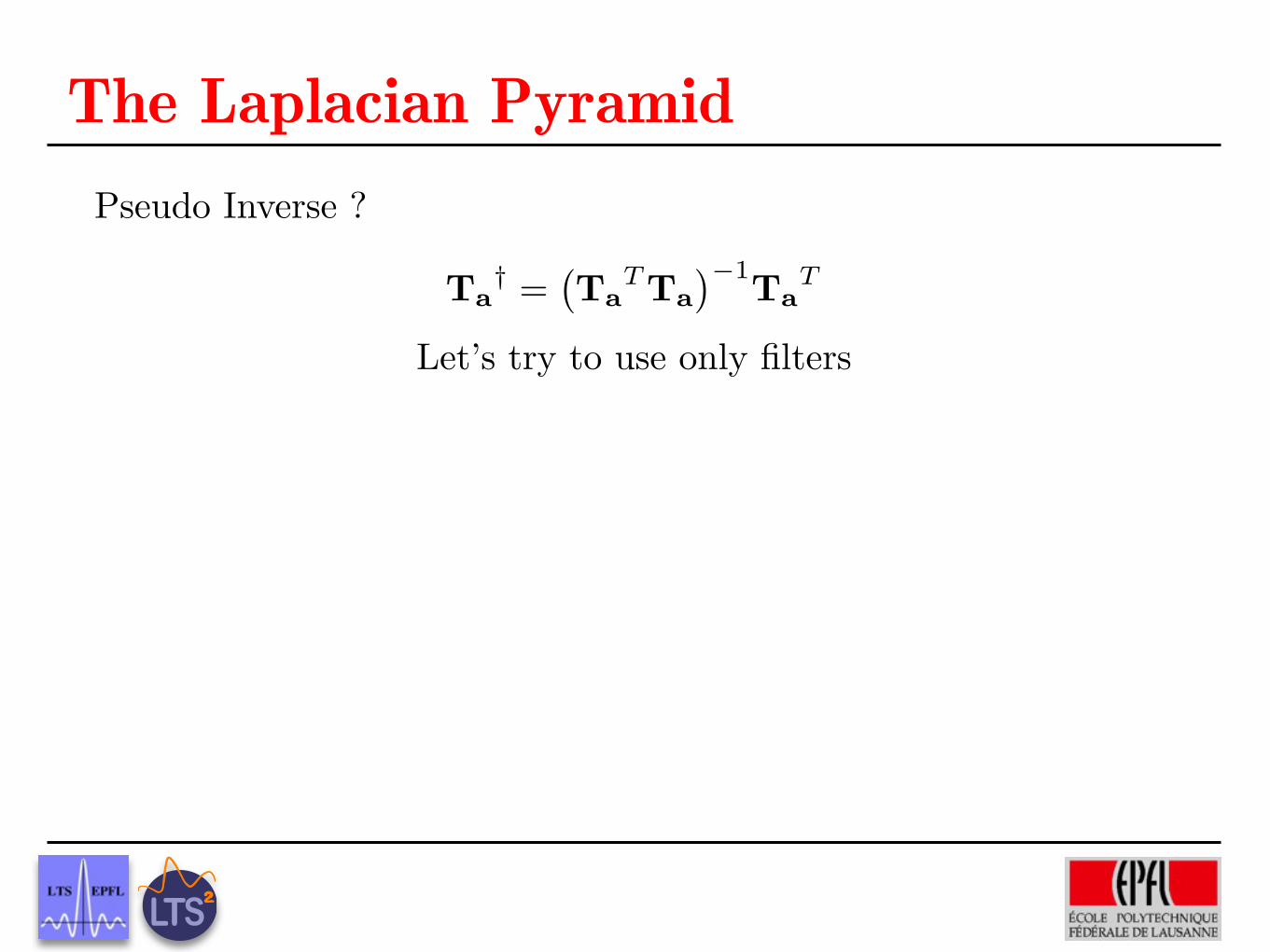
Ta† =
�Ta
T Ta
��1TaT
The Laplacian PyramidPseudo Inverse ?
Let’s try to use only filters
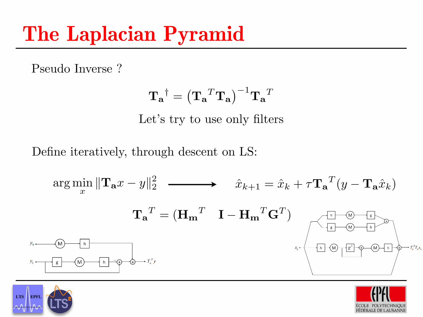
Ta† =
�Ta
T Ta
��1TaT
The Laplacian PyramidPseudo Inverse ?
Let’s try to use only filters
arg minx
kTax� yk22 xk+1 = xk + ⌧Ta
T (y �Taxk)
TaT = (Hm
T I�HmT GT )
Define iteratively, through descent on LS:
Figure 5.3: Complementary operator TaT for synthesis part of the graph LP.
Figure 5.4: Complementary operator TaTT for synthesis part of the graph
LP.
Figure 5.5: Iterative reconstruction of the graph-signal using gradient descentmethod.
34
Figure 5.3: Complementary operator TaT for synthesis part of the graph LP.
Figure 5.4: Complementary operator TaTT for synthesis part of the graph
LP.
Figure 5.5: Iterative reconstruction of the graph-signal using gradient descentmethod.
34
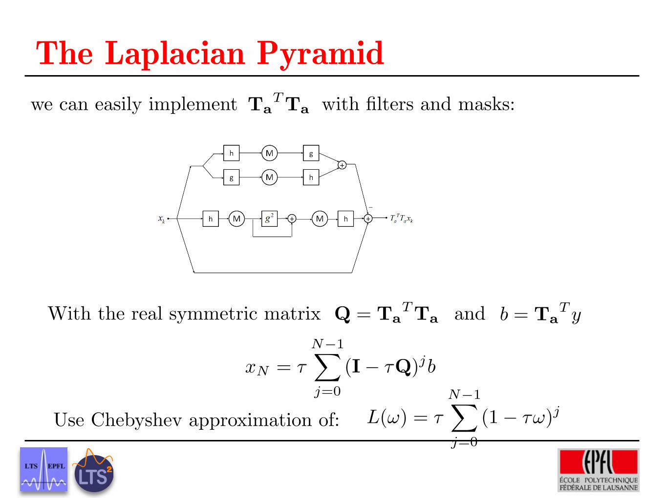
TaT Ta
Q = TaT Ta b = Ta
T y
xN = ⌧
N�1X
j=0
(I� ⌧Q)jb
L(!) = ⌧N�1X
j=0
(1� ⌧!)j
The Laplacian PyramidFigure 5.3: Complementary operator Ta
T for synthesis part of the graph LP.
Figure 5.4: Complementary operator TaTT for synthesis part of the graph
LP.
Figure 5.5: Iterative reconstruction of the graph-signal using gradient descentmethod.
34
we can easily implement with filters and masks:
With the real symmetric matrix and
Use Chebyshev approximation of:
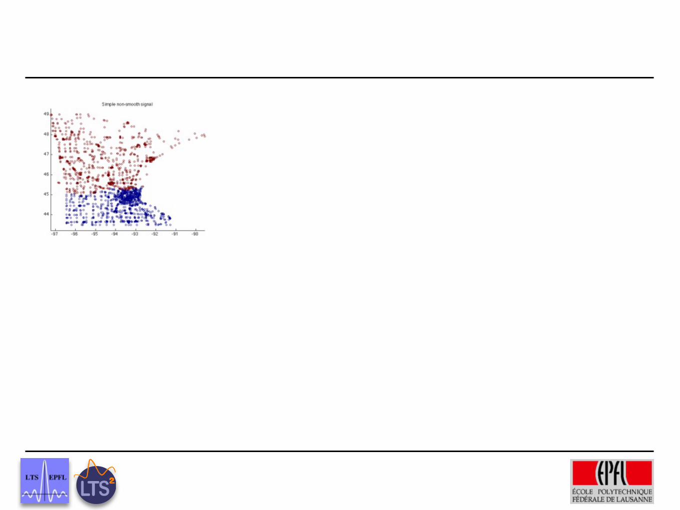

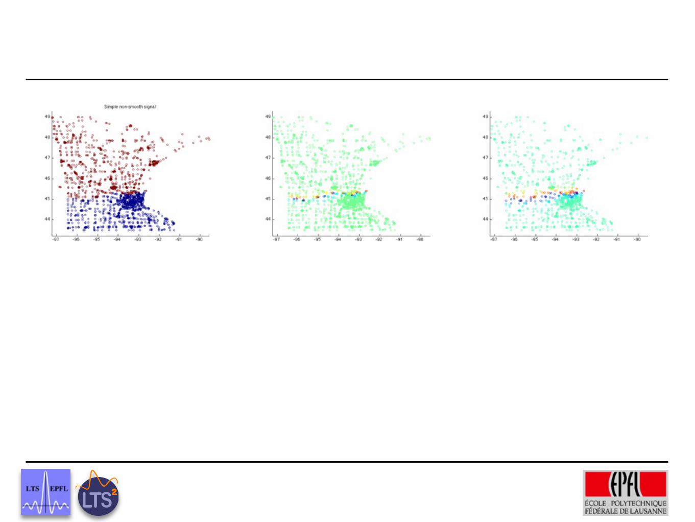
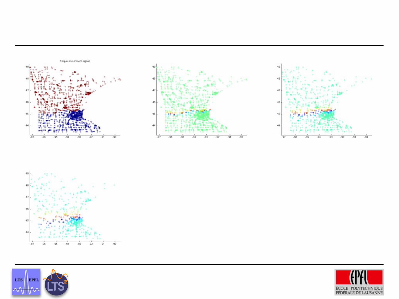
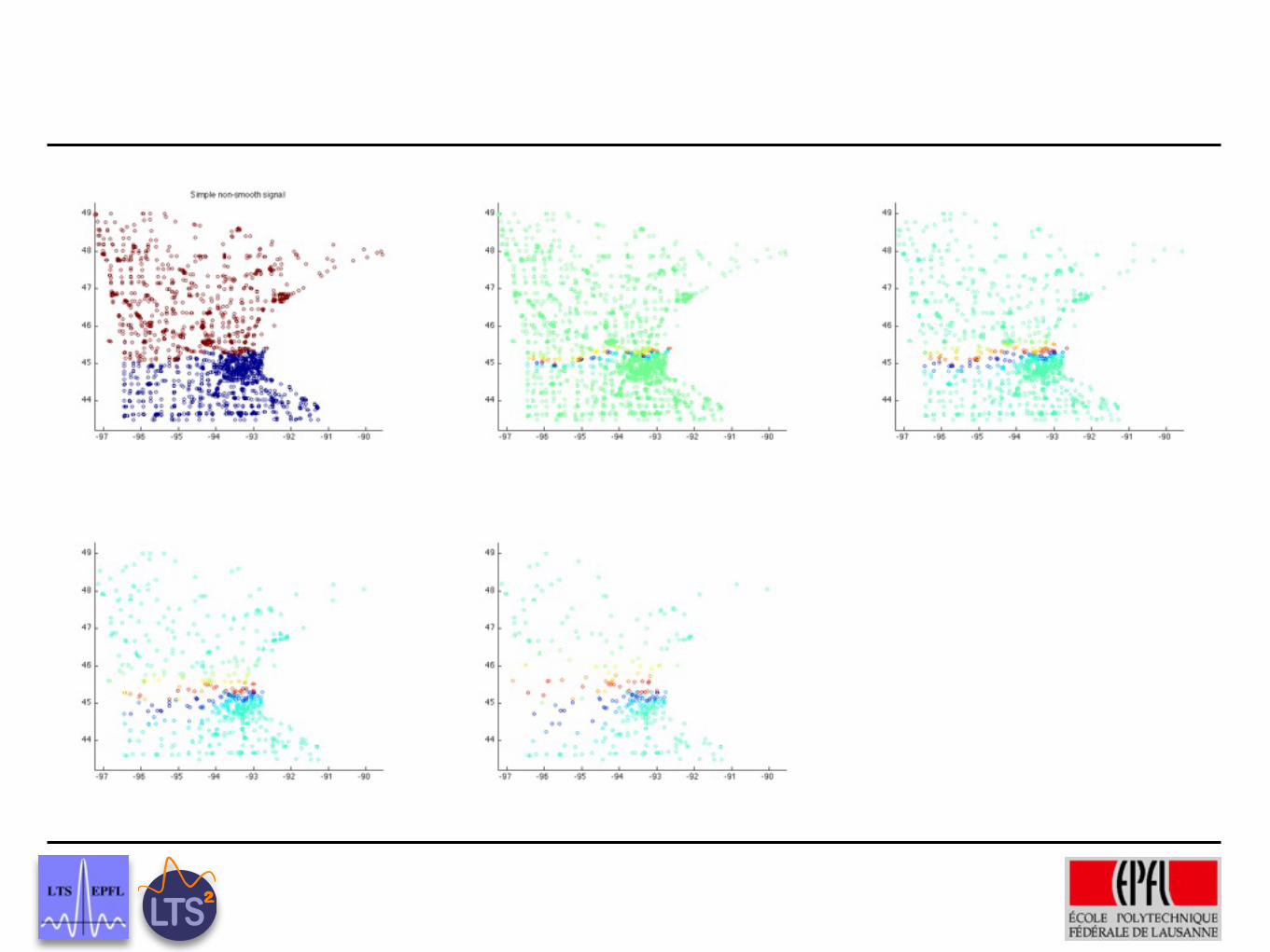
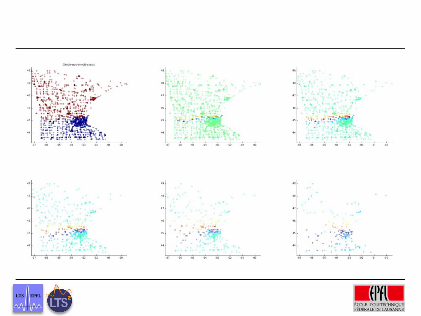
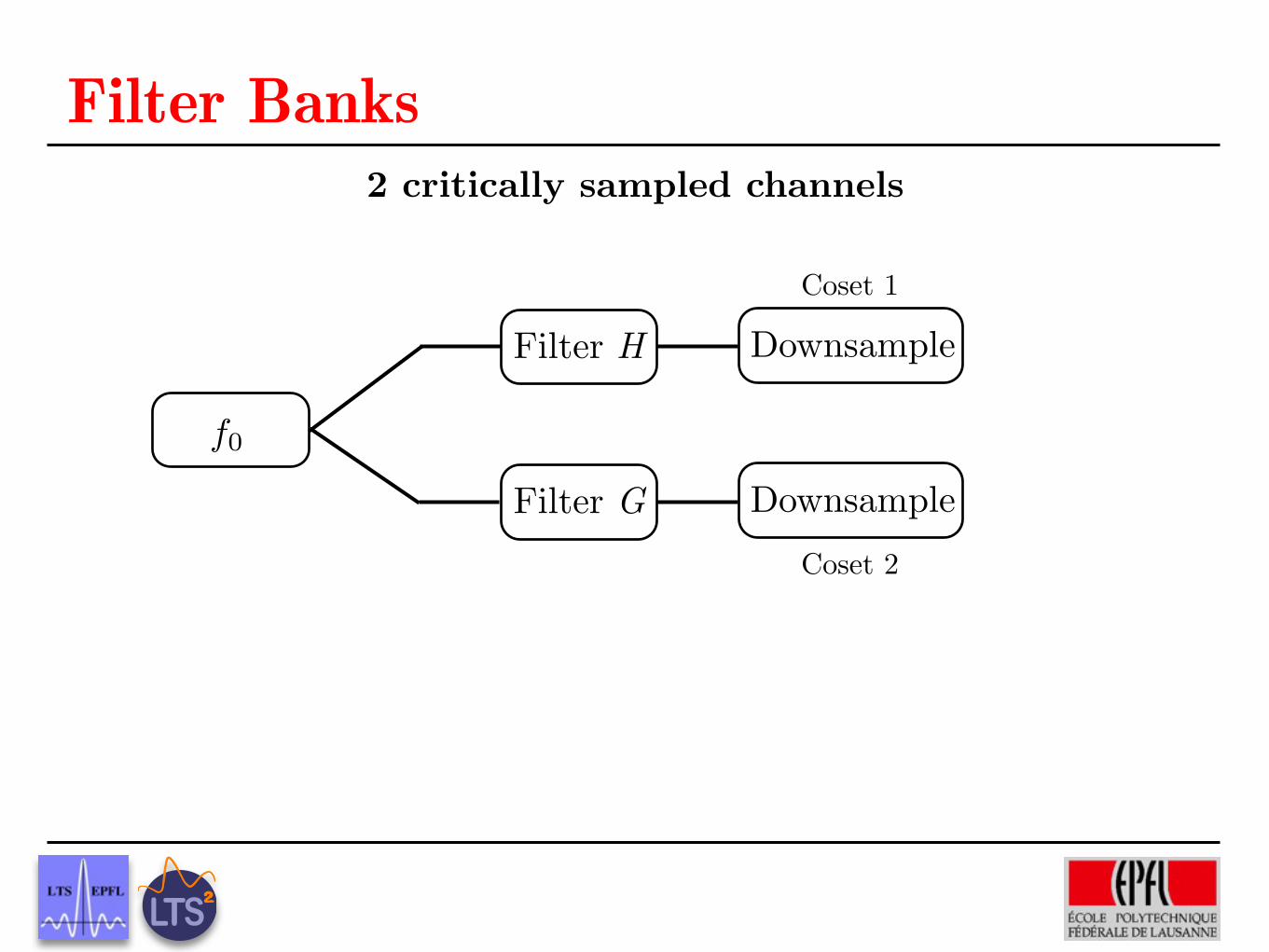
f0
Filter Banks2 critically sampled channels
Filter H
Filter G
Downsample
Downsample
Coset 1
Coset 2
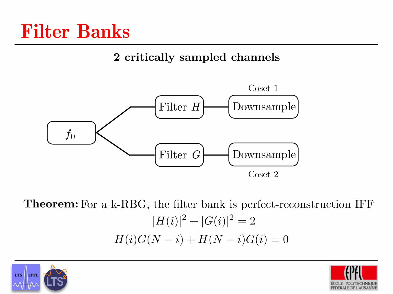
f0
Filter Banks2 critically sampled channels
Filter H
Filter G
Downsample
Downsample
Coset 1
Coset 2
|H(i)|2 + |G(i)|2 = 2
H(i)G(N � i) + H(N � i)G(i) = 0
Theorem: For a k-RBG, the filter bank is perfect-reconstruction IFF
Intro Spectral Graph Theory Wavelets on Graphs Chebyshev Approximation Distributed Processing Open Issues
Outline
1 Introduction
2 Spectral Graph Theory Background
3 Wavelet Constructions on Graphs
4 Approximate Graph Multiplier Operators
5 Distributed Signal Processing via the Chebyshev Approximation
6 Open Issues and Challenges
Vandergheynst and Shuman (EPFL) Wavelets on Graphs November 17, 2011 59 / 76
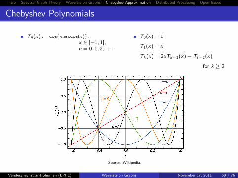
Intro Spectral Graph Theory Wavelets on Graphs Chebyshev Approximation Distributed Processing Open Issues
Chebyshev Polynomials
Tn(x) := cos(n arccos(x)
),
x ∈ [−1, 1],n = 0, 1, 2, . . .
T0(x) = 1
T1(x) = x
Tk (x) = 2xTk−1(x)− Tk−2(x)
for k ≥ 2
Source: Wikipedia.
Vandergheynst and Shuman (EPFL) Wavelets on Graphs November 17, 2011 60 / 76
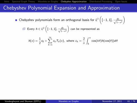
Intro Spectral Graph Theory Wavelets on Graphs Chebyshev Approximation Distributed Processing Open Issues
Chebyshev Polynomial Expansion and Approximation
Chebyshev polynomials form an orthogonal basis for L2
([−1, 1], dx√
1−x2
)� Every h ∈ L2
([−1, 1], dx√
1−x2
)can be represented as
h(x) =1
2c0 +
∞∑k=1
ckTk (x), where ck =2
π
∫ π
0cos(kθ)h(cos(θ))dθ
K th order Chebyshev approximation to a continuous function on aninterval provides a near-optimal approximation (in the sup norm) amongstall polynomials of degree K
Shifted Chebyshev Polynomials
� To shift the domain from [-1,1] to [0,A], define
T k (x) := Tk
( x
α− 1), where α :=
A
2
� T k (x) = 2α
(x − α)T k−1(x)− T k−2(x) for k ≥ 2
Vandergheynst and Shuman (EPFL) Wavelets on Graphs November 17, 2011 61 / 76
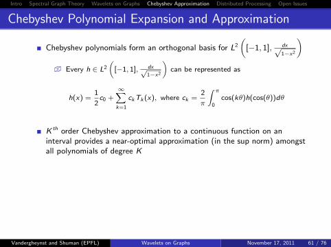
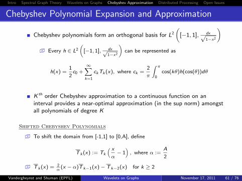
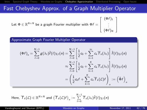
Intro Spectral Graph Theory Wavelets on Graphs Chebyshev Approximation Distributed Processing Open Issues
Fast Chebyshev Approx. of a Graph Multiplier Operator
Let Φ ∈ RN×N be a graph Fourier multiplier with Φf =
(Φf )1
...(Φf )N
Approximate Graph Fourier Multiplier Operator
(Φf )n =N−1∑`=0
g(λ`)f (`)χ`(n) =N−1∑`=0
[1
2c0 +
∞∑k=1
ckT k(λ`)
]f (`)χ`(n)
≈N−1∑`=0
[1
2c0 +
K∑k=1
ckT k(λ`)
]f (`)χ`(n)
=
(1
2c0f +
K∑k=1
ckT k(L)f
)n
:=(
Φf)
n
Here, T k(L) ∈ RN×N and(T k(L)f
)n
:=N−1∑
=0
T k(λ`)f (`)χ`(n)
Vandergheynst and Shuman (EPFL) Wavelets on Graphs November 17, 2011 62 / 76
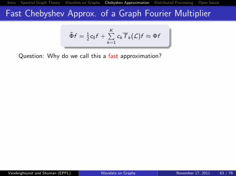
Intro Spectral Graph Theory Wavelets on Graphs Chebyshev Approximation Distributed Processing Open Issues
Fast Chebyshev Approx. of a Graph Fourier Multiplier
Φf = 12c0f +
K∑k=1
ckT k(L)f ≈ Φf
Question: Why do we call this a fast approximation?
Answer: From the Chebyshev polynomial recursion property, we have:
T 0(L)f = f
T 1(L)f =1
αLf − f , where α :=
λmax
2
T k(L)f =2
α(L − αI )
(T k−1(L)f
)− T k−2(L)f
=2
αLT k−1(L)f − 2T k−1(L)f − T k−2(L)f
Does not require explicit computation of the eigenvectors of the Laplacian
Computational cost proportional to # nonzero entries in the Laplacian
This corresponds to the number of edges in the communication graph
Large, sparse graph ⇒ Φf far more efficient than Φf
Vandergheynst and Shuman (EPFL) Wavelets on Graphs November 17, 2011 63 / 76
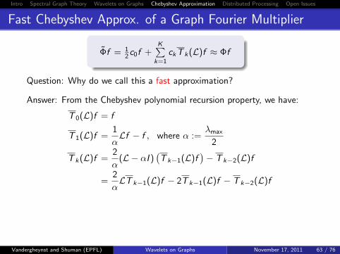
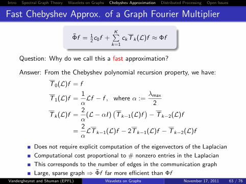
Intro Spectral Graph Theory Wavelets on Graphs Chebyshev Approximation Distributed Processing Open Issues
Fast Chebyshev Approx. of a Graph Fourier Multiplier
Φf = 12c0f +
K∑k=1
ckT k(L)f ≈ Φf
Question: Why do we call this a fast approximation?
Answer: From the Chebyshev polynomial recursion property, we have:
T 0(L)f = f
T 1(L)f =1
αLf − f , where α :=
λmax
2
T k(L)f =2
α(L − αI )
(T k−1(L)f
)− T k−2(L)f
=2
αLT k−1(L)f − 2T k−1(L)f − T k−2(L)f
Does not require explicit computation of the eigenvectors of the Laplacian
Computational cost proportional to # nonzero entries in the Laplacian
This corresponds to the number of edges in the communication graph
Large, sparse graph ⇒ Φf far more efficient than ΦfVandergheynst and Shuman (EPFL) Wavelets on Graphs November 17, 2011 63 / 76
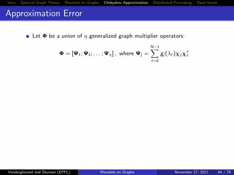
Intro Spectral Graph Theory Wavelets on Graphs Chebyshev Approximation Distributed Processing Open Issues
Approximation Error
Let Φ be a union of η generalized graph multiplier operators:
Φ = [Ψ1; Ψ2; . . . ; Ψη] , where Ψj =N−1∑`=0
gj(λ`)χ`χ∗`
Define B(K) := maxj=1,2,...,η
{sup
λ∈[0,λmax]
{∣∣gj(λ)− pKj (λ)
∣∣}}
Proposition
|||Φ− Φ|||2 := maxf 6=0
‖(Φ−Φ)f‖2‖f‖2
≤ B(K)√ηN.
Proposition (see, e.g., Mason and Handscomb, 2003)
If gj(·) has M + 1 continuous derivatives for all j , then B(K) = O(K−M
).
Vandergheynst and Shuman (EPFL) Wavelets on Graphs November 17, 2011 64 / 76
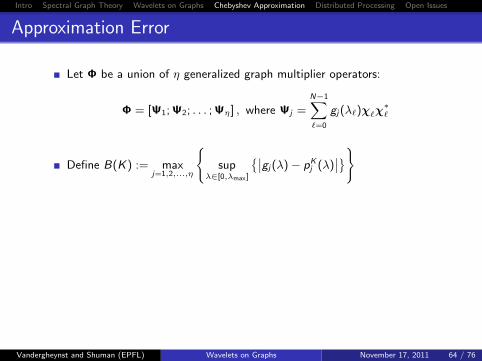
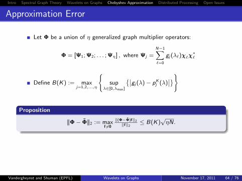
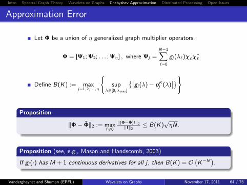
Intro Spectral Graph Theory Wavelets on Graphs Chebyshev Approximation Distributed Processing Open Issues
Outline
1 Introduction
2 Spectral Graph Theory Background
3 Wavelet Constructions on Graphs
4 Approximate Graph Multiplier Operators
5 Distributed Signal Processing via the Chebyshev Approximation
6 Open Issues and Challenges
Vandergheynst and Shuman (EPFL) Wavelets on Graphs November 17, 2011 65 / 76
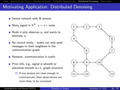
Intro Spectral Graph Theory Wavelets on Graphs Chebyshev Approximation Distributed Processing Open Issues
Motivating Application: Distributed Denoising
Sensor network with N sensors
Noisy signal in RN : y = x+ noise
Node n only observes yn and wants toestimate xn
No central entity - nodes can only sendmessages to their neighbors in thecommunication graph
However, communication is costly
Prior info, e.g., signal is smooth or
piecewise smooth w.r.t. graph structure
� If two sensors are close enough to
communicate, their observations are
more likely to be correlated
?>=<89:;1 //
��
?>=<89:;2 //oo ?>=<89:;3
AAAAAAAAoo
?>=<89:;4
AAAAAAAA
OO
?>=<89:;5
``AAAAAAAA
��?>=<89:;6
��
``AAAAAAAA ?>=<89:;7
~~}}}}}}}
OO
?>=<89:;8 //
��
?>=<89:;9
��
OO
oo // ?>=<89:;10oo
>>}}}}}}}
AAAAAAA
?>=<89:;11
OO
// ?>=<89:;12
OO
oo ?>=<89:;13
``AAAAAAA
Vandergheynst and Shuman (EPFL) Wavelets on Graphs November 17, 2011 66 / 76
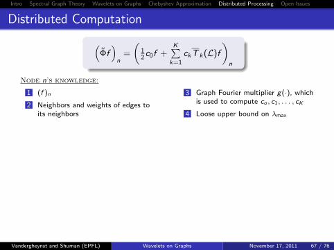
Intro Spectral Graph Theory Wavelets on Graphs Chebyshev Approximation Distributed Processing Open Issues
Distributed Computation
(Φf)
n=
(12c0f +
K∑k=1
ckT k(L)f
)n
Node n’s knowledge:
1 (f )n
2 Neighbors and weights of edges toits neighbors
3 Graph Fourier multiplier g(·), whichis used to compute co , c1, . . . , cK
4 Loose upper bound on λmax
Task: Compute (T k(L)f )n, k ∈ {1, 2, . . . ,K} in a distributed manner
(T 1(L)f )n = 1α
(Lf )n − (f )n = 1α
f0 Ln,2 0 0 0 Ln,6 0 0 0 −(f )n
(T k (L)f
)n
=(
2αLT k−1(L)f
)n−(
2T k−1(L)f)
n−(T k−2(L)f
)n
To get (T 2(L)f )n, suffices to compute (LT 1(L)f )n = `T1(L)f0 Ln,2 0 0 0 Ln,6 0 0 0
2K |E |scalar
messages
Vandergheynst and Shuman (EPFL) Wavelets on Graphs November 17, 2011 67 / 76
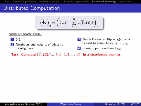
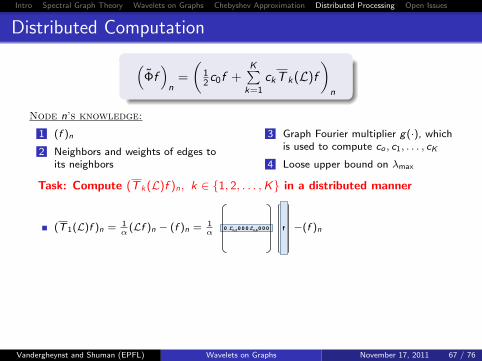
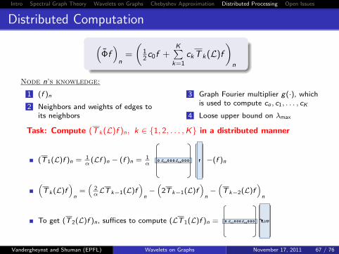
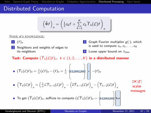
Intro Spectral Graph Theory Wavelets on Graphs Chebyshev Approximation Distributed Processing Open Issues
Distributed Denoising - Method 1
Prior: signal is smooth w.r.t the underlying graph structure
Regularization term: fTLf = 12
∑n∈V
∑m∼n
wm,n [f (m)− f (n)]2
� fTLf = 0 iff f is constant across all vertices
� fTLf is small when signal f has similar values at neighboring vertices
connected by an edge with a large weight
Distributed regularization problem:
argminf
τ
2‖f − y‖2
2 + fTLf (1)
Proposition
The solution to (1) is given by Ry, where R is a graph Fourier multiplieroperator with multiplier g(λ`) = τ
τ+2λ`.
Vandergheynst and Shuman (EPFL) Wavelets on Graphs November 17, 2011 68 / 76
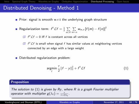
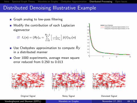
Intro Spectral Graph Theory Wavelets on Graphs Chebyshev Approximation Distributed Processing Open Issues
Distributed Denoising Illustrative Example
Graph analog to low-pass filtering
Modify the contribution of each Laplacian
eigenvector
� f∗(n) = (Ry)n =N−1∑
=0
[τ
τ+2λ`
]y(`)χ`(n)
Use Chebyshev approximation to compute Ryin a distributed manner
Over 1000 experiments, average mean squareerror reduced from 0.250 to 0.013
0 5 10 150
0.1
0.2
0.3
0.4
0.5
0.6
0.7
0.8
0.9
1
λ
Exact MultiplierChebyshev Polynomial Approximation, K=5Chebyshev Polynomial Approximation, K=15
Original Signal Noisy Signal Denoised Signal
Vandergheynst and Shuman (EPFL) Wavelets on Graphs November 17, 2011 69 / 76
Intro Spectral Graph Theory Wavelets on Graphs Chebyshev Approximation Distributed Processing Open Issues
Distributed Denoising - Method 2
Prior: signal is p.w. smooth w.r.t. graph ⇔ SGWT coefficients sparse
Regularize via LASSO (Tibshirani, 1996):
mina
12‖y −W ∗a‖2
2 + µ‖a‖1
Solve via iterative soft thresholding (Daubechies et al., 2004):
a(β) = Sµτ(a(β−1) + τW
(y −W ∗a(β−1)
)), β = 1, 2, . . .
D-LASSO (Mateos et al., 2010) solves in distributed fashion, but requires2|E | messages of length N(J + 1) at each iteration
We solve the LASSO with the approximate wavelet operator via thedistributed Chebyshev computation method
The communication workload only scales with network size through |E |,otherwise independent of N
‖W ∗a∗ −W ∗a∗‖22 ≤
‖y‖32
µ
√N(J + 1)B(K)
Vandergheynst and Shuman (EPFL) Wavelets on Graphs November 17, 2011 70 / 76
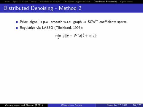
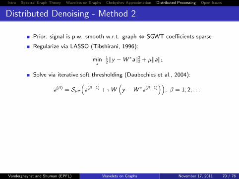
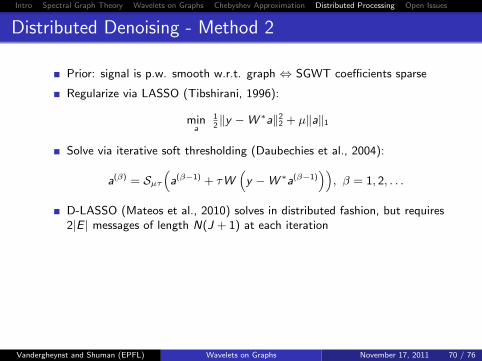
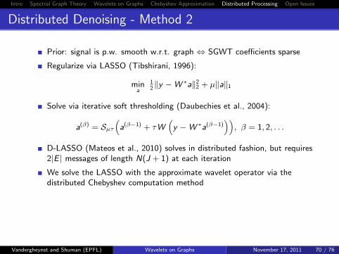
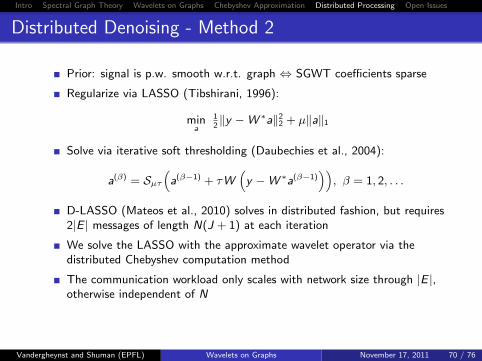
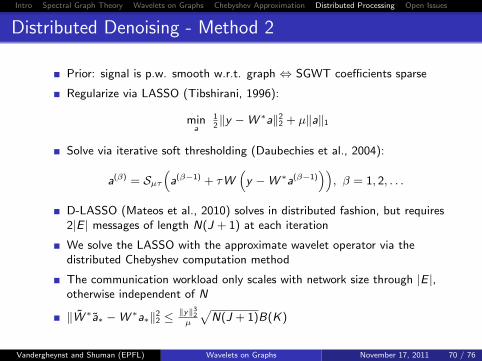
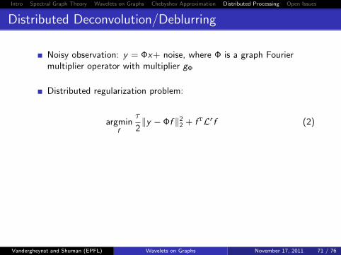
Intro Spectral Graph Theory Wavelets on Graphs Chebyshev Approximation Distributed Processing Open Issues
Distributed Deconvolution/Deblurring
Noisy observation: y = Φx+ noise, where Φ is a graph Fouriermultiplier operator with multiplier gΦ
Distributed regularization problem:
argminf
τ
2‖y − Φf ‖2
2 + fTLr f (2)
Proposition
The solution to (2) is given by Ry, where R is a graph Fourier multiplier
operator with multiplier g(λ`) = τgΦ(λ`)τg2
Φ(λ`)+2λr`.
Compute Ry in a distributed manner
Vandergheynst and Shuman (EPFL) Wavelets on Graphs November 17, 2011 71 / 76
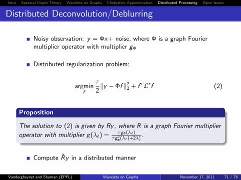
Intro Spectral Graph Theory Wavelets on Graphs Chebyshev Approximation Distributed Processing Open Issues
Distributed Semi-Supervised Classification
Finite number of classes {1, 2, . . . ,C}
We know the class labels for l vertices on the graph (l << N)
Want to determine the labels for the other vertices in a distributed manner
Many centralized solutions (e.g., Zhou et al., 2004) force the labels to besmooth with respect to the intrinsic structure of the graph by
argmaxj∈{1,2,...,κ}
F optnj , where Fopt is the solution to
Fopt = argminF∈RN×κ
κ∑j=1
{τ‖F:,j − Y:,j‖2
2 + ‖F:,j‖2H}
� ‖f‖2H = 〈f, f〉H := 〈f,Pf〉 = fTPf for different choices
of real, symmetric, positive semi-definite matrices P
0 1 0
0 0 0
κ
l
.
.
.
1 0 0
N
…
0 0 1
0 0 0
0 0 0
u
Y =
Vandergheynst and Shuman (EPFL) Wavelets on Graphs November 17, 2011 72 / 76
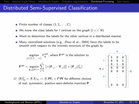
Intro Spectral Graph Theory Wavelets on Graphs Chebyshev Approximation Distributed Processing Open Issues
Distributed Semi-Supervised Classification (cont’d)
Equivalent to κ separate minimization problems:
Fopt:,j = argmin
f∈RN
{τ‖f − Y:,j‖2
2 + fTPf}
(3)
Solution to (3) is given by RY:,j , where R is a generalized graphmultiplier operator (with respect to P) with a multiplier of τ
τ+λ
This type of framework provides a way to distribute a number of existing(centralized) semi-supervised classification and regression methods fromthe machine learning literature
Vandergheynst and Shuman (EPFL) Wavelets on Graphs November 17, 2011 73 / 76
Intro Spectral Graph Theory Wavelets on Graphs Chebyshev Approximation Distributed Processing Open Issues
Summary
A number of distributed signal processing tasks can be represented asapplications of graph multiplier operators
We approximate the graph multipliers by Chebyshev polynomials
The recurrence relations of the Chebyshev polynomials make theapproximate operators readily amenable to distributed computation
The communication required to perform distributed computations onlyscales with the size of the network through the number of edges in thecommunication graph
The proposed method is well-suited to large-scale networks with sparsecommunication graphs
Vandergheynst and Shuman (EPFL) Wavelets on Graphs November 17, 2011 74 / 76
Intro Spectral Graph Theory Wavelets on Graphs Chebyshev Approximation Distributed Processing Open Issues
Outline
1 Introduction
2 Spectral Graph Theory Background
3 Wavelet Constructions on Graphs
4 Approximate Graph Multiplier Operators
5 Distributed Signal Processing via the Chebyshev Approximation
6 Open Issues and Challenges
Vandergheynst and Shuman (EPFL) Wavelets on Graphs November 17, 2011 75 / 76
Intro Spectral Graph Theory Wavelets on Graphs Chebyshev Approximation Distributed Processing Open Issues
Further Reading
Spectral Graph Theory, Laplacian Eigenvectors, and Nodal Domains
F. K. Chung, Spectral Graph Theory. Vol. 92 of the CBMS Regional Conference Series in Mathematics,AMS Bokstore, 1997.
T. Bıyıkoglu, J. Leydold, and P. F. Stadler, Laplacian Eigenvectors of Graphs. Lecture Notes inMathematics, vol. 1915, Springer, 2007.
Spectral Clustering
U. von Luxburg, “A tutorial on spectral clustering,” Stat. Comput., vol. 17, no. 4, pp. 395–416, 2007.
Chebyshev Polynomials
J. C. Mason and D. C. Handscomb, Chebyshev Polynomials. Chapman and Hall, 2003.
Spectral Graph Wavelet Transform and Distributed Processing
D. K. Hammond, P. Vandergheynst, and R. Gribonval, “Wavelets on graphs via spectral graph theory,”
Appl. Comput. Harmon. Anal., vol. 30, no. 2, pp. 129–150, Mar. 2011.
D. I Shuman, P. Vandergheynst, and P. Frossard, “Chebyshev polynomial approximation for distributed
signal processing,”in Proc. Int. Conf. Distr. Comput. Sensor Sys. (DCOSS), Barcelona, Spain, Jun. 2011.
Vandergheynst and Shuman (EPFL) Wavelets on Graphs November 17, 2011 76 / 76
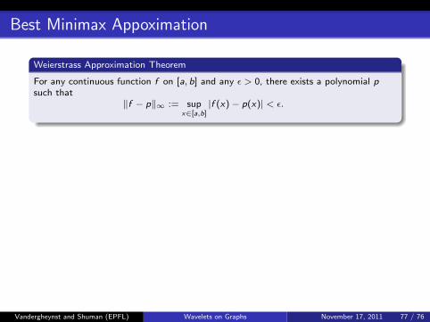
Best Minimax Appoximation
Weierstrass Approximation Theorem
For any continuous function f on [a, b] and any ε > 0, there exists a polynomial psuch that
‖f − p‖∞ := supx∈[a,b]
|f (x)− p(x)| < ε.
� Catch: The degree of the approximating polynomial may be large
� What is the best we can do when the degree of the approximating polynomial isbounded?
� Consider approximation space Pn, with elements pn(x) = a0 + a1x + . . .+ anxn
Questions
1 Does there exist p∗n ∈ Pn such that ‖f − p∗n ‖∞ = infpn∈Pn
‖f − pn‖∞?
Yes
2 If so, is it unique?
Yes
3 What are the characteristic properties of p∗n ?
4 How do we compute p∗n ?
Vandergheynst and Shuman (EPFL) Wavelets on Graphs November 17, 2011 77 / 76
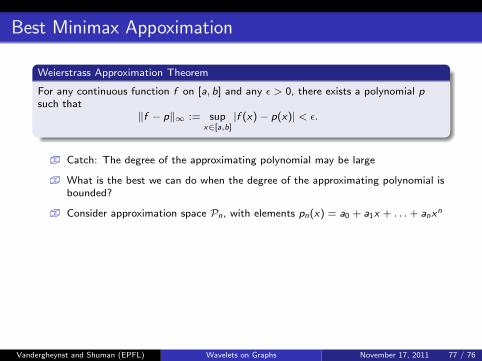
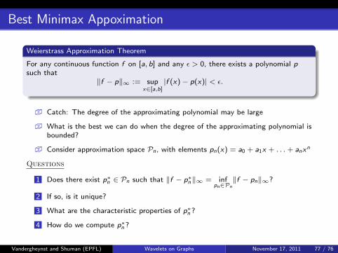
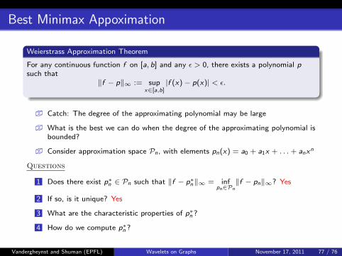
Best Minimax Appoximation
Weierstrass Approximation Theorem
For any continuous function f on [a, b] and any ε > 0, there exists a polynomial psuch that
‖f − p‖∞ := supx∈[a,b]
|f (x)− p(x)| < ε.
� Catch: The degree of the approximating polynomial may be large
� What is the best we can do when the degree of the approximating polynomial isbounded?
� Consider approximation space Pn, with elements pn(x) = a0 + a1x + . . .+ anxn
Questions
1 Does there exist p∗n ∈ Pn such that ‖f − p∗n ‖∞ = infpn∈Pn
‖f − pn‖∞? Yes
2 If so, is it unique? Yes
3 What are the characteristic properties of p∗n ?
4 How do we compute p∗n ?
Vandergheynst and Shuman (EPFL) Wavelets on Graphs November 17, 2011 77 / 76
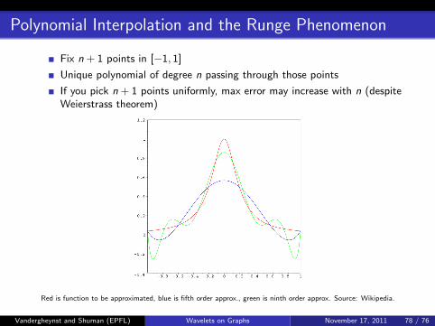
Polynomial Interpolation and the Runge Phenomenon
Fix n + 1 points in [−1, 1]
Unique polynomial of degree n passing through those points
If you pick n + 1 points uniformly, max error may increase with n (despiteWeierstrass theorem)
Red is function to be approximated, blue is fifth order approx., green is ninth order approx. Source: Wikipedia.
Vandergheynst and Shuman (EPFL) Wavelets on Graphs November 17, 2011 78 / 76
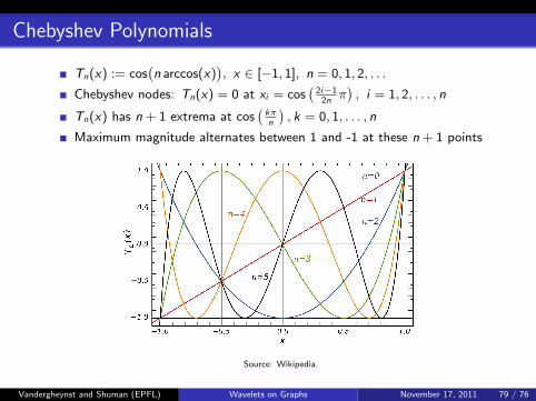
Chebyshev Polynomials
Tn(x) := cos(n arccos(x)
), x ∈ [−1, 1], n = 0, 1, 2, . . .
Chebyshev nodes: Tn(x) = 0 at xi = cos(
2i−12nπ), i = 1, 2, . . . , n
Tn(x) has n + 1 extrema at cos(
kπn
), k = 0, 1, . . . , n
Maximum magnitude alternates between 1 and -1 at these n + 1 points
Source: Wikipedia.
Vandergheynst and Shuman (EPFL) Wavelets on Graphs November 17, 2011 79 / 76
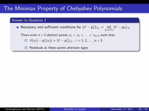
The Minimax Property of Chebyshev Polynomials
Answer to Question 3
Necessary and sufficient conditions for ‖f − p∗n ‖∞ = infpn∈Pn
‖f − pn‖∞
There exist n + 2 distinct points x1 < x2 < . . . < xn+2 such that:
� |f (xi )− p∗n (xi )| = ‖f − p∗n ‖∞ , i = 1, 2, . . . , n + 2
� Residuals at these points alternate signs
Application: argminpn−1∈Pn−1
‖xn − pn−1‖∞ = xn − 12n−1 Tn(x)
Answer to Question 4
Polynomial interpolation with the n + 1 points chosen to be the Chebyshevnodes (zeros) of Tn+1(x)
Puts more of the interpolation points towards the ends than uniform choice
Can iterate by setting new interpolation points to be those with the largestmagnitude of error in previous round
Near-optimal and the error decreases as you consider higher degree polynomials
Vandergheynst and Shuman (EPFL) Wavelets on Graphs November 17, 2011 80 / 76
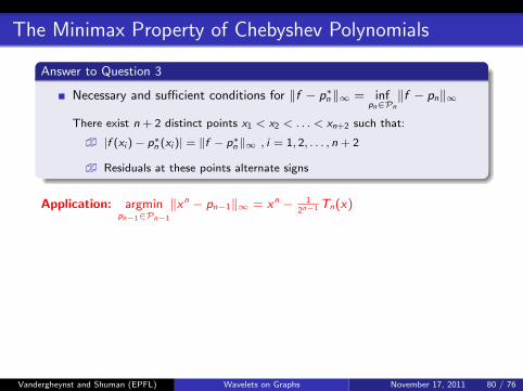
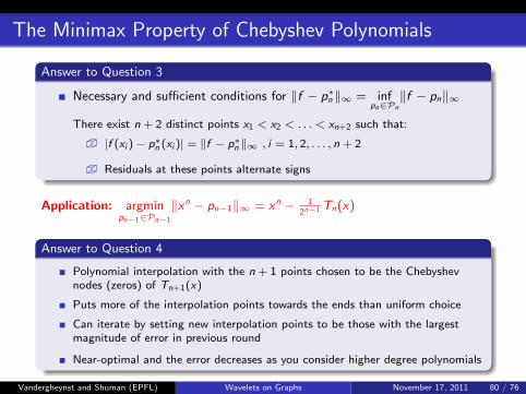
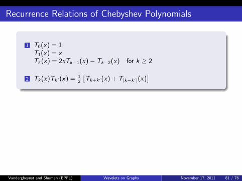
Recurrence Relations of Chebyshev Polynomials
1 T0(x) = 1T1(x) = xTk(x) = 2xTk−1(x)− Tk−2(x) for k ≥ 2
2 Tk(x)Tk′(x) = 12
[Tk+k′(x) + T|k−k′|(x)
]
Shifted Chebyshev Polynomials
� To shift the domain from [-1,1] to [0,A], define
T k(x) := Tk
( x
α− 1), where α :=
A
2
� T k(x) = 2α (x − α)T k−1(x)− T k−2(x) for k ≥ 2
Vandergheynst and Shuman (EPFL) Wavelets on Graphs November 17, 2011 81 / 76
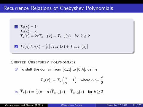
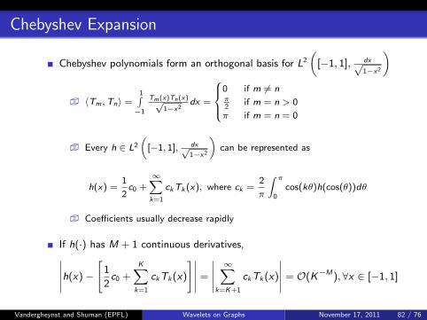
Chebyshev Expansion
Chebyshev polynomials form an orthogonal basis for L2
([−1, 1], dx√
1−x2
)
� 〈Tm,Tn〉 =1∫−1
Tm(x)Tn(x)√1−x2
dx =
0 if m 6= nπ2
if m = n > 0
π if m = n = 0
� Every h ∈ L2
([−1, 1], dx√
1−x2
)can be represented as
h(x) =1
2c0 +
∞∑k=1
ckTk (x), where ck =2
π
∫ π
0cos(kθ)h(cos(θ))dθ
� Coefficients usually decrease rapidly
If h(·) has M + 1 continuous derivatives,∣∣∣∣∣h(x)−
[1
2c0 +
K∑k=1
ckTk(x)
]∣∣∣∣∣ =
∣∣∣∣∣∞∑
k=K+1
ckTk(x)
∣∣∣∣∣ = O(K−M), ∀x ∈ [−1, 1]
Vandergheynst and Shuman (EPFL) Wavelets on Graphs November 17, 2011 82 / 76


![机器学习讨论班 - wds.ac.cnwds.ac.cn/portal/summer2019/ppt/11.pdf[1] Defferrard M, Bresson X, Vandergheynst P. Convolutional neural networks on graphs with fast localized spectral](https://img.pdfslide.net/doc/110x75/602bb7b7827b6962653d49a7/oeeec-wdsaccnwdsaccnportalsummer2019ppt11pdf-1-defferrard.jpg)