Embed Size (px)
Citation preview
WAVELETS
RONALD A. DeVORE and BRADLEY J. LUCIER
1. Introduction
The subject of “wavelets” is expanding at such a tremendous rate that it isimpossible to give, within these few pages, a complete introduction to all aspects ofits theory. We hope, however, to allow the reader to become sufficiently acquaintedwith the subject to understand, in part, the enthusiasm of its proponents towardits potential application to various numerical problems. Furthermore, we hope thatour exposition can guide the reader who wishes to make more serious excursions intothe subject. Our viewpoint is biased by our experience in approximation theory anddata compression; we warn the reader that there are other viewpoints that are eithernot represented here or discussed only briefly. For example, orthogonal waveletswere developed primarily in the context of signal processing, an application whichwe touch on only indirectly. However, there are several good expositions (e.g.,[Da1] and [RV]) of this application. A discussion of wavelet decompositions inthe context of Littlewood-Paley theory can be found in the monograph of Frazier,Jawerth, and Weiss [FJW]. We shall also not attempt to give a complete discussionof the history of wavelets. Historical accounts can be found in the book of Meyer[Me] and the introduction of the article of Daubechies [Da1]. We shall try to giveenough historical commentary in the course of our presentation to provide somefeeling for the subject’s development.
The term “wavelet” (originally called wavelet of constant shape) was introducedby J. Morlet. It denotes a univariate function ψ (multivariate wavelets exist as welland will be discussed subsequently), defined on R, which, when subjected to thefundamental operations of shifts (i.e., translation by integers) and dyadic dilation,yields an orthogonal basis of L2(R). That is, the functions ψj,k := 2k/2ψ(2k· − j),j, k ∈ Z, form a complete orthonormal system for L2(R). In this work, weshall call such a function an orthogonal wavelet, since there are many general-izations of wavelets that drop the requirement of orthogonality. The Haar functionH := χ[0,1/2) − χ[1/2,1), which will be discussed in more detail in the section thatfollows, is the simplest example of an orthogonal wavelet. Orthogonal wavelets withhigher smoothness (and even compact support) can also be constructed. But beforeconsidering that and other questions, we wish first to motivate the desire for suchwavelets.
A version of this paper appeared in Acta Numerica, A. Iserles, ed., Cambridge University
Press, v. 1 (1992), pp. 1–56. This work was supported in part by the National Science Foundation(grants DMS-8922154 and DMS-9006219), the Air Force Office of Scientific Research (contract
89-0455-DEF), the Office of Naval Research (contracts N00014-90-1343, N00014-91-J-1152, and
N00014-91-J-1076), the Defense Advanced Research Projects Agency (AFOSR contract 90-0323),and the Army High Performance Computing Research Center at the University of Minnesota.
1
2 RONALD A. DEVORE AND BRADLEY J. LUCIER
−1 0 1
φ
j − 1
2kj
2kj + 1
2k
φ(2k· − j)
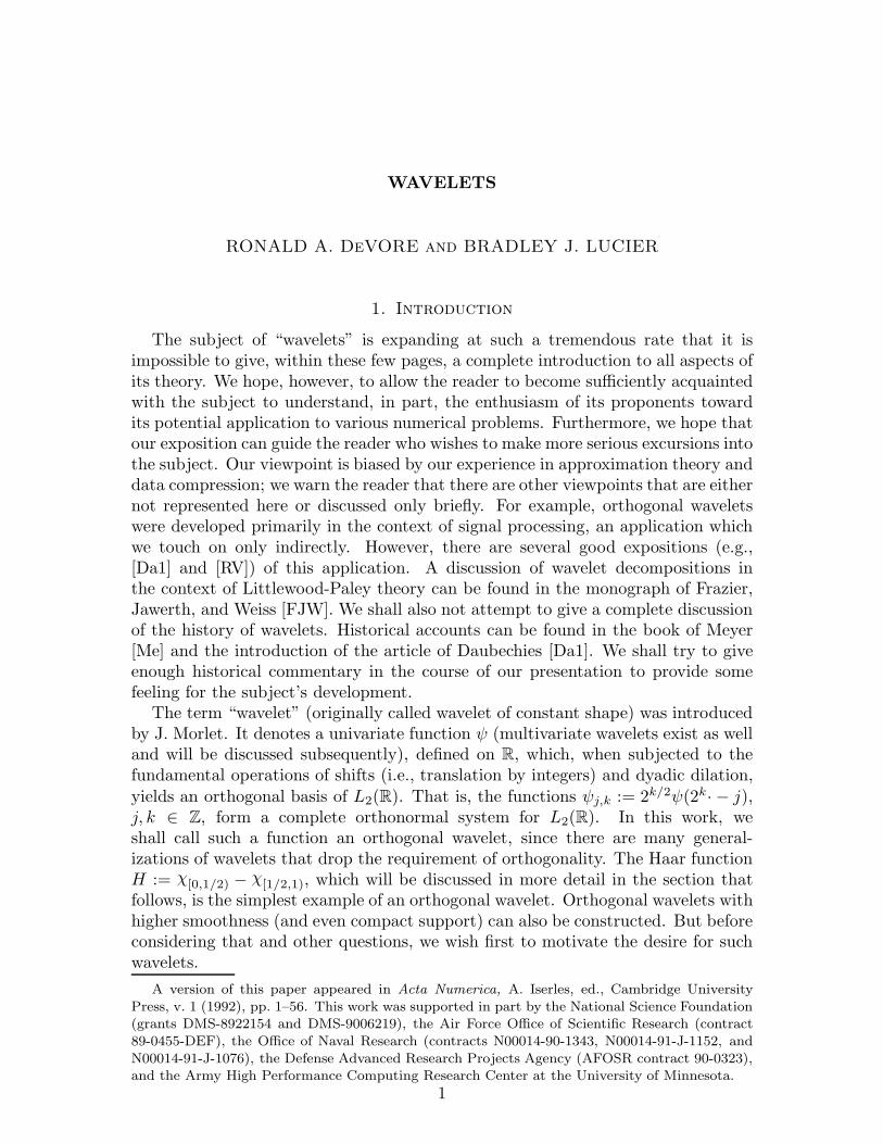
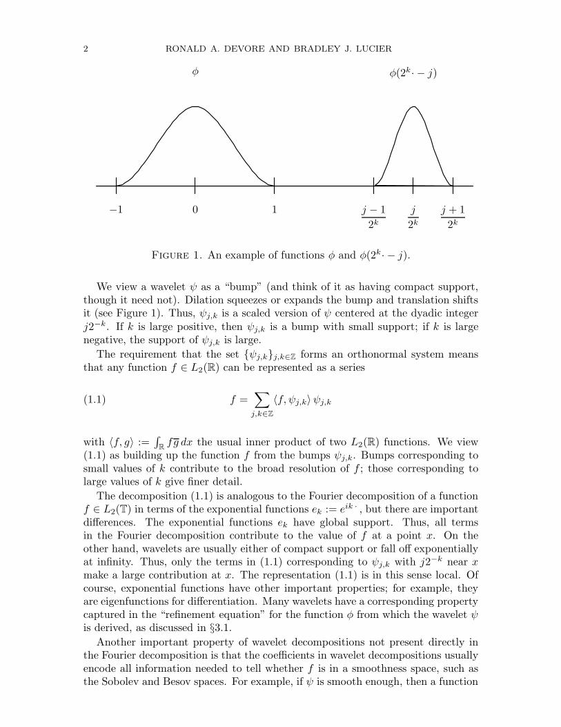
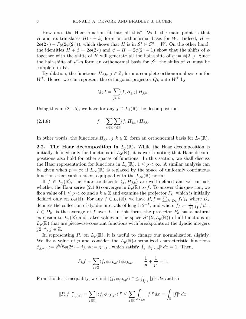
Figure 1. An example of functions φ and φ(2k· − j).
We view a wavelet ψ as a “bump” (and think of it as having compact support,though it need not). Dilation squeezes or expands the bump and translation shiftsit (see Figure 1). Thus, ψj,k is a scaled version of ψ centered at the dyadic integerj2−k. If k is large positive, then ψj,k is a bump with small support; if k is largenegative, the support of ψj,k is large.
The requirement that the set ψj,kj,k∈Z forms an orthonormal system meansthat any function f ∈ L2(R) can be represented as a series
(1.1) f =∑
j,k∈Z
〈f, ψj,k〉ψj,k
with 〈f, g〉 :=∫Rfg dx the usual inner product of two L2(R) functions. We view
(1.1) as building up the function f from the bumps ψj,k. Bumps corresponding tosmall values of k contribute to the broad resolution of f ; those corresponding tolarge values of k give finer detail.
The decomposition (1.1) is analogous to the Fourier decomposition of a functionf ∈ L2(T) in terms of the exponential functions ek := eik · , but there are importantdifferences. The exponential functions ek have global support. Thus, all termsin the Fourier decomposition contribute to the value of f at a point x. On theother hand, wavelets are usually either of compact support or fall off exponentiallyat infinity. Thus, only the terms in (1.1) corresponding to ψj,k with j2−k near xmake a large contribution at x. The representation (1.1) is in this sense local. Ofcourse, exponential functions have other important properties; for example, theyare eigenfunctions for differentiation. Many wavelets have a corresponding propertycaptured in the “refinement equation” for the function φ from which the wavelet ψis derived, as discussed in §3.1.
Another important property of wavelet decompositions not present directly inthe Fourier decomposition is that the coefficients in wavelet decompositions usuallyencode all information needed to tell whether f is in a smoothness space, such asthe Sobolev and Besov spaces. For example, if ψ is smooth enough, then a function
WAVELETS 3
f is in the Lipschitz space Lip(α, L∞(R)), 0 < α < 1, if and only if
(1.2) supj,k
2k(α+12)|〈f, ψj,k〉|
is finite, and (1.2) is an equivalent seminorm for Lip(α, L∞(R)).All this would be of little more than theoretical interest if it were not for the
fact that one can efficiently compute wavelet coefficients and reconstruct functionsfrom these coefficients. Such algorithms, known as “fast wavelet transforms” arethe analogue of the Fast Fourier Transform and follow simply from the refinementequation mentioned above.
In many numerical applications, the orthogonality of the translated dilates ψj,kis not vital. There are many variants of wavelets, such as the prewavelets proposedby Battle [Ba] and the φ-transform of Frazier and Jawerth [FJ], that do not requireorthogonality. Typically, for a given function ψ, one wants the translated dilatesψj,k, j, k ∈ Z, to form a stable basis (also called a Riesz basis) for L2(R). Thismeans that each f ∈ L2(R) has a unique series decomposition in terms of the ψj,k,and that the ℓ2 norm of the coefficients in this series is equivalent to ‖f‖L2(R) (thiswill be discussed in more detail in §3.1). In other applications, when approximatingin L1(R), for example, one must abandon the requirement that ψj,k, j, k ∈ Z, forma stable basis of L1(R), because none exists. (The Haar system is a Schauder basisfor L1([0, 1]), for example, but the representation is not L1([0, 1])-stable.) For suchapplications, one can use redundant representations of f , with ψ a box spline, forexample.
We have, to this point, restricted our discussion to univariate wavelets. Thereare several constructions of multivariate wavelets but the final form of this theoryis yet to be decided. We shall discuss two methods for constructing multivariatewavelets; one is based on tensor products while the other is truly multivariate.
The plan of the paper is as follows. Section 2 is meant to introduce the topicof wavelets by studying the simplest orthogonal wavelets, which are the Haar func-tions. We discuss the decomposition of Lp(R) using the Haar expansion, the char-acterization of certain smoothness spaces in terms of the coefficients in the Haarexpansion, the fast Haar transform, and multivariate Haar functions. Section 3concerns itself with the construction of wavelets. It begins with a discussion ofthe properties of shift-invariant spaces, and then gives an overview of the construc-tion of univariate wavelets and prewavelets within the framework of multiresolution.Later, mention is made of Daubechies’ specific construction of orthonormal waveletsof compact support. We finish with a discussion of wavelets in several dimensions.
Section 4 examines how to calculate the coefficients of wavelet expansions viathe so-called Fast Wavelet Transform. Section 5 is concerned with the characteri-zation of functions in certain smoothness classes called Besov spaces in terms of thesize of wavelet coefficients. Section 6 turns to numerical applications. We brieflymention some uses of wavelets in nonlinear approximation, data compression (and,more specifically, image compression), and numerical methods for partial differen-tial equations.
2. The Haar Wavelets
2.1. Overview. The Haar functions are the most elementary wavelets. While
4 RONALD A. DEVORE AND BRADLEY J. LUCIER
they have many drawbacks, chiefly their lack of smoothness, they still illustrate inthe most direct way some of the main features of wavelet decompositions. For thisreason, we shall consider in some detail the properties that make them suitable fornumerical applications. We hope that the detail we provide at this stage will rendermore convincing some of the later statements we make, without proof, about moregeneral wavelets.
We consider first the univariate case. Let H := χ[0,1/2) − χ[1/2,1) be the Haarfunction that takes the value 1 on the left half of [0, 1] and the value −1 on theright half. By translation and dilation, we form the functions
(2.1.1) Hj,k := 2k/2H(2k· − j), j, k ∈ Z.
Then, Hj,k is supported on the dyadic interval Ij,k := [j2−k, (j + 1)2−k).It is easy to see that these functions form an orthonormal system. In fact,
given two of these functions Hj,k, Hj′,k′ , k′ ≥ k and (j, k) 6= (j′, k′), we have
two possibilities. The first is that the dyadic intervals Ij,k and Ij′,k′ are disjoint,in which case
∫RHj,kHj′,k′ = 0 (because the integrand is identically zero). The
second possibility is that k′ > k and Ij′,k′ is contained in one of the halves J of Ij,k.In this case Hj,k is constant on J while Hj′,k′ takes the values ±1 equally often onits support. Hence, again
∫RHj,kHj′,k′ = 0.
We want next to show that Hj,k | j, k ∈ Z is complete in L2(R). The followingdevelopment gives us a chance to introduce the concept of multiresolution, whichis the main vehicle for constructing wavelets and which will be discussed in moredetail in the section that follows. Let S := S0 denote the subspace of L2(R) thatconsists of all piecewise-constant functions with integer breakpoints; i.e., functionsin S are constant on each interval [j, j+1), j ∈ Z. Then S is a shift-invariant space:if S ∈ S, each of its shifts, S( · + k), k ∈ Z, is also in S. A simple orthonormalbasis for S is given by the shifts of the function φ := χ[0,1]. Namely, each S ∈ Shas a unique representation
(2.1.2) S =∑
j∈Z
c(j)φ( · − j), (c(j)) ∈ ℓ2(Z).
By dilation, we can form a scale of spaces
Sk := S(2k · ) | S ∈ S, k ∈ Z.
Thus, Sk is the space of piecewise-constant L2(R) functions with breakpoints atthe dyadic integers j2−k. The normalized dyadic shifts φj,k := 2k/2φ(2k· − j) =
2k/2φ(2k( · − j2−k)) with step j2−k, j ∈ Z, of the function φ(2k · ), form an or-thonormal basis for Sk. However, to avoid possible confusion, we note that thetotality of all such functions φj,k is not a basis for the space L2(R) because there
is redundancy. For example, φ = (φ0,1 + φ1,1)/√2.
Clearly, we have Sk ⊂ Sk+1, k ∈ Z, so the spaces Sk get “thicker” as k getslarger and “thinner” as k gets smaller. We are interested in the limiting spaces
(2.1.3) S∞ :=⋃
Sk and S−∞ :=⋂
Sk,
WAVELETS 5
since these spaces hold the key to showing that the Haar basis is complete. Weclaim that
(2.1.4) S∞ = L2(R) and S−∞ = 0.
The first of these claims is equivalent to the fact that any function in L2(R) canbe approximated arbitrarily well (in the L2(R) norm) by the piecewise-constantfunctions from Sk provided k is large enough. For example, it is enough to ap-proximate f by its best L2(R) approximation from Sk. This best approximation isgiven by the orthogonal projector Pk from L2(R) onto Sk. It is easy to see that
Pkf(x) =1
|Ij,k|
∫
Ij,k
f, x ∈ Ij,k, j ∈ Z.
To verify the second claim in (2.1.4), we suppose that f ∈ ⋂Sk. Then, f isconstant on each of (−∞, 0) and [0,∞), and since f ∈ L2(R), we must have f = 0a.e. on each of these intervals.
Now, consider again the projector Pk from L2(R) onto Sk. By (2.1.4), Pkf → f ,k → ∞. We also claim that Pkf → 0, k → −∞. Indeed, if this were false, then wecould find a C > 0 and a subsequence mj → −∞ for which ‖Pmj
f‖L2(R) ≥ C forall mj . By the weak-∗ compactness of L2(R), we can also assume that Pmj
f → g,weak-∗, for some g ∈ L2(R). Now, for any m ∈ Z, all Pmj
f are in Sm for mj
sufficiently large and negative. Since Sm is weak-∗ closed, g ∈ Sm. Hence g ∈ ⋂Smimplies g = 0 a.e. This gives a contradiction because by orthogonality
∫
R
|Pmjf |2 dx =
∫
R
fPmjf dx→
∫
R
fg dx = 0.
It follows that each f ∈ L2(R) can be represented by the series
(2.1.5) f =∑
k∈Z
(Pkf − Pk−1f) =∑
k∈Z
Qkf, Qk−1 := Pk − Pk−1
because the partial sums, Pnf − P−nf , of this series tend to f as n→ ∞.To complete the construction of the Haar wavelets, we need the following simple
remarks about projections. If Y ⊂ X are two closed subspaces of L2(R) and PXand PY are the orthogonal projectors onto these spaces, then Q := PX − PY is theorthogonal projector from L2(R) onto X⊖Y , the orthogonal complement of Y in X(this follows from the identity PY PX = PY ). Thus, the operator Qk−1 := Pk−Pk−1
appearing in (2.1.5) is the orthogonal projector onto W k−1 := Sk ⊖ Sk−1. Thespaces W k are the dilates of the wavelet space
(2.1.6) W := S1 ⊖ S0.
Since the spaces W k, k ∈ Z, are mutually orthogonal, we have W k ⊥ W j, j 6= k,and (2.1.5) shows that L2(R) is the orthogonal direct sum of the W k:
(2.1.7) L2(R) =⊕
k∈Z
W k.
6 RONALD A. DEVORE AND BRADLEY J. LUCIER
How does the Haar function fit into all this? Well, the main point is thatH and its translates H( · − k) form an orthonormal basis for W . Indeed, H =2φ(2 · )− P0(2φ(2 · )), which shows that H is in S1 ⊖ S0 =W . On the other hand,the identities H + φ = 2φ(2 · ) and φ − H = 2φ(2 · − 1) show that the shifts of φtogether with the shifts of H will generate all the half-shifts of η := φ(2 · ). Since
the half-shifts of√2 η form an orthonormal basis for S1, the shifts of H must be
complete in W .By dilation, the functions Hj,k, j ∈ Z, form a complete orthonormal system for
W k. Hence, we can represent the orthogonal projector Qk onto W k by
Qkf =∑
j∈Z
〈f,Hj,k〉Hj,k.
Using this in (2.1.5), we have for any f ∈ L2(R) the decomposition
(2.1.8) f =∑
k∈Z
∑
j∈Z
〈f,Hj,k〉Hj,k.
In other words, the functions Hj,k, j, k ∈ Z, form an orthonormal basis for L2(R).
2.2. The Haar decomposition in Lp(R). While the Haar decomposition isinitially defined only for functions in L2(R), it is worth noting that Haar decom-positions also hold for other spaces of functions. In this section, we shall discussthe Haar representation for functions in Lp(R), 1 ≤ p <∞. A similar analysis canbe given when p = ∞ if L∞(R) is replaced by the space of uniformly continuousfunctions that vanish at ∞, equipped with the L∞(R) norm.
If f ∈ Lp(R), the Haar coefficients 〈f,Hj,k〉 are well defined and we can askwhether the Haar series (2.1.8) converges in Lp(R) to f . To answer this question, wefix a value of 1 ≤ p <∞ and a k ∈ Z and examine the projector Pk, which is initiallydefined only on L2(R). For any f ∈ L2(R), we have Pkf =
∑I∈Dk
fIχI where Dkdenotes the collection of dyadic intervals of length 2−k, and where fI :=
1|I|
∫If dx,
I ∈ Dk, is the average of f over I. In this form, the projector Pk has a naturalextension to Lp(R) and takes values in the space Sk(χ, Lp(R)) of all functions inLp(R) that are piecewise-constant functions with breakpoints at the dyadic integersj2−k, j ∈ Z.
In representing Pk on Lp(R), it is useful to change our normalization slightly.We fix a value of p and consider the Lp(R)-normalized characteristic functions
φj,k,p := 2k/pφ(2k· − j), φ := χ[0,1], which satisfy∫R|φj,k,p|p dx = 1. Then,
Pkf =∑
j∈Z
〈f, φj,k,p′〉φj,k,p,1
p+
1
p′= 1.
From Holder’s inequality, we find |〈f, φj,k,p′〉|p ≤∫Ij,k
|f |p dx and so
‖Pkf‖pLp(R)=
∑
j∈Z
|〈f, φj,k,p′〉|p ≤∑
j∈Z
∫
Ij,k
|f |p dx =
∫
R
|f |p dx.
WAVELETS 7
Therefore, Pk is a bounded operator with norm 1 on the space Lp(R).If f ∈ Lp(R), then since Pk is a projector of norm one,
(2.2.1) ‖f − Pkf‖Lp(R) = infS∈Sk
‖(I − Pk)(f − S)‖Lp(R) ≤ 2 dist(f,Sk)Lp(R).
It follows that Pkf → f in Lp(R) for each f ∈ Lp(R).On the other hand, consider Pkf as k → −∞. If f is continuous and of compact
support then at most 2 terms in Pkf are nonzero for k large negative and eachcoefficient is ≤ C2k/p
′
. Hence ‖Pkf‖Lp(R) → 0 provided p′ < ∞, i.e., p > 1. Thisshows that
(2.2.2) f =∑
k∈Z
(Pkf − Pk−1f) =∑
k∈Z
∑
j∈Z
〈f,Hj,k〉Hj,k.
in the sense of Lp(R) convergence. We see that the Haar representation holds forfunctions in Lp(R) provided p > 1.
But what happens when p = 1? Well, as is typical for orthogonal decompositions,the expansion (2.2.2) cannot be valid. Indeed, each of the functions appearing onthe right in (2.2.2) has mean value zero. If g ∈ L1(R) has mean value zero and f isan arbitrary function from L1(R), then
∫
R
|f − g| dx ≥ |∫
R
f dx−∫
R
g dx| = |∫
R
f dx|.
This means that the sum in (2.2.2) cannot possibly converge in L1(R) to f unlessf has mean value zero.
The above phenomenon is typical of decompositions for orthogonal wavelets ψ:They cannot represent all functions in L1(R). However, if ψ is smooth enough, therepresentation (2.2.2) will hold for the Hardy space H1(R) used in place of L1(R),and in fact this representation will then hold for functions in the Hardy spacesHp(R) for a certain range of 0 < p < 1 that depends on the smoothness of ψ. Weshall not discuss further the behavior of orthogonal wavelets in Hp spaces but theinterested reader can consult Frazier and Jawerth [FJ] for a corresponding theoryin a slightly different setting.
2.3. Smoothness spaces. We noted earlier the important fact that wavelet de-compositions provide a description of smoothness spaces in terms of the waveletcoefficients. We wish to illustrate this point with the Haar wavelets and the Lip-schitz spaces in Lp(R), 1 < p <∞.
The Lipschitz spaces Lip(α, Lp(R)) of Lp(R), 0 < α ≤ 1, 1 ≤ p ≤ ∞, consist ofall functions f ∈ Lp(R) for which
‖f − f( · + h)‖Lp(R) = O(hα), h→ 0.
A seminorm for this space is provided by
|f |Lip(α,Lp(R)) := sup0<h<∞
h−α‖f − f( · + h)‖Lp(R).
8 RONALD A. DEVORE AND BRADLEY J. LUCIER
The relationship between the smoothness of f and the size of its Haar coefficientsrests on three fundamental inequalities. The first of these says that for a fixed k ∈ Z,the Haar functions Hj,k, j ∈ Z, are Lp(R)-stable. Because of the disjoint supportof the Hj,k, j ∈ Z, stability takes the following particularly simple form: for anysequence (c(j)) ∈ ℓp(Z) and S =
∑j∈Z
c(j)Hj,k, we have
(2.3.1) ‖S‖Lp(R) =
(∑
j∈Z
|c(j)|p2kp(1/2−1/p)
)1/p
.
This follows by integrating the identity
|S|p =∑
j∈Z
|c(j)|p|Hj,k|p.
The other two inequalities are related to the approximation properties of Sk andthe projectors Pk:(2.3.2)
(J) ‖f − Pkf‖Lp(R) ≤ 2 · 2−kα|f |Lip(α,Lp(R)), 0 < α ≤ 1, 1 ≤ p ≤ ∞.
(B) |S|Lip(1/p,Lp(R)) ≤ 2 · 2k/p‖S‖Lp(R), S ∈ Sk(χ, Lp(R)), 1 ≤ p ≤ ∞.
The first of these, often called a Jackson inequality (after similar inequalities estab-lished by D. Jackson for polynomial approximation), tells how well functions fromLip(α, Lp(R)) can be approximated by the elements of Sk. The second inequal-ity is known as a Bernstein inequality because of its similarity with the classicalBernstein inequalities for polynomials, established by S. Bernstein.
We shall prove (2.3.2) (J) and (B) for 1 ≤ p <∞. If I ∈ Dk and h := |I| = 2−k,then, for all x ∈ I, we obtain
|f(x)− fI | ≤1
|I|
∫
I
|f(x)− f(y)| dy
≤(
1
|I|
∫
I
|f(x)− f(y)|p dy)1/p
≤(
1
|I|
∫ h
−h
|f(x)− f(x+ s)|p ds)1/p
.
If we raise these last inequalities to the power p, integrate over I, and then sumover all I ∈ Dk, we obtain
‖f − Pkf‖pLp(R)≤ 1
h
∫ h
−h
∫
R
|f(x)− f(x+ s)|p dx ds ≤ 2|h|αp|f |pLip(α,Lp(R)),
which implies the Jackson inequality.The Jackson inequality can also be proved from more general principles. Since
the Pk have norm 1 on Lp(R) and are projectors, we have
(2.3.3) ‖f − Pkf‖Lp(R) ≤ (1 + ‖Pk‖) dist(f,Sk)Lp(R) ≤ 2 dist(f,Sk)Lp(R).
Thus, the Jackson inequality follows from the fact that functions in Lip(α, Lp(R))can be approximated by the elements of Sk with an error not exceeding the rightside of (2.3.2)(J).
WAVELETS 9
To prove the Bernstein inequality, we note that any S =∑j∈Z
c(j)χIj,k in
Sk(χ, Lp(R)) has norm:
(2.3.4) ‖S‖pLp(R)=
∑
j∈Z
|c(j)|p|Ij,k| =∑
j∈Z
|c(j)|p2−k.
We fix an h > 0. If h ≥ 2−k (i.e., h−1/p ≤ 2k/p), then
h−1/p‖S( · + h) − S‖Lp(R) ≤ 2k/p(‖S( · + h)‖Lp(R) + ‖S‖Lp(R)) = 2 · 2k/p‖S‖Lp(R).
If h < 2−k then
|S(x+ h)− S(x)| =
0, x ∈ [j2−k, (j + 1)2−k − h),
|c(j + 1)− c(j)|, x ∈ [(j + 1)2−k − h, (j + 1)2−k).
Therefore
h−1/p‖S( · + h) − S‖Lp(R) = h−1/p
(∑
j∈Z
|c(j + 1)− c(j)|ph)1/p
= 2k/p(∑
j∈Z
|c(j + 1)− c(j)|p2−k)1/p
= 2k/p‖S( · + 2−k)− S‖Lp(R) ≤ 2 · 2k/p‖S‖Lp(R).
With the Jackson and Bernstein inequalities in hand, it is now easy to show that
(2.3.5) |f |Lip(α,Lp(R)) ≈ supk∈Z
2k(α+1/2−1/p)
(∑
j∈Z
|〈f,Hj,k〉|p)1/p
, 0 < α < 1/p.
(It will be convenient to use the notation A ≈ B to mean that the two ratios A/Band B/A of the functions A and B are bounded from above independently of thevariables; in (2.3.5), independently of f .) First, from the Jackson inequality,
‖Pkf −Pk−1f‖Lp(R) ≤ ‖f −Pkf‖Lp(R) + ‖f −Pk−1f‖Lp(R) ≤ C 2−kα|f |Lip(α,Lp(R)).
If we write Pkf−Pk−1f =∑j∈Z
〈f,Hj,k−1〉Hj,k−1 and replace ‖Pkf−Pk−1f‖Lp(R)
by the sum in (2.3.1) (with c(j) = 〈f,Hj,k−1〉), we obtain that the right side of(2.3.5) does not exceed a multiple of the left.
To reverse this inequality, we fix a value of h and choose n ∈ Z so that 2−n ≤h ≤ 2−n+1. We write f =
∑k∈Z
wk with wk := (Pk+1f − Pkf) and estimate
(2.3.6) ‖f( · + h) − f‖Lp(R)
≤∑
k≥n
‖wk( · + h)− wk‖Lp(R) +∑
k<n
‖wk( · + h)− wk‖Lp(R).
10 RONALD A. DEVORE AND BRADLEY J. LUCIER
The first sum does not exceed(supk≥n
2kα‖wk‖Lp(R)
)(∑
k≥n
2−kα)
≤ Chα supk≥n
2kα‖wk‖Lp(R).
Similarly, using the Bernstein inequality, the second sum does not exceed
h1/p∑
k<n
|wk|Lip(1/p,Lp(R)) ≤ C h1/p∑
k<n
2k/p‖wk‖Lp(R)
≤ C h1/p(supk<n
2kα‖wk‖Lp(R)
)(∑
k<n
2k(1/p−α))
≤ C hα supk<n
2kα‖wk‖Lp(R).
If we write wk =∑j∈Z
〈f,Hj,k〉Hj,k and use (2.3.1) to replace ‖wk‖Lp(R) by
2k(1/2−1/p)
(∑
j∈Z
|〈f,Hj,k〉|p)1/p
in each of these expressions, and then use the resulting expression in (2.3.6), weobtain
‖f( · + h)− f‖Lp(R) ≤ Chα supk∈Z
2k(α+1/2−1/p)
(∑
j∈Z
|〈f,Hj,k〉|p)1/p
,
which shows that the left side of (2.3.5) does not exceed a multiple of the right.The restriction α < 1/p arises because the Haar function is not smooth; for
smoother wavelets, the range of α can be increased.
2.4. The fast Haar transform. In numerical applications of the Haar decompo-sition, one must work with only a finite number of the functions Hj,k. The choiceof which functions to use is often made as follows. Given a function f ∈ L2(R), wechoose a large value of n, compatible with the accuracy we wish to achieve, andwe replace f by Pnf with Pn, as before, the L2(R) projector onto Sn, the spaceof piecewise-constant functions in L2(R) with breakpoints at the dyadic integersj2−n, j ∈ Z. If f has compact support then Pnf is a finite linear combination ofthe characteristic functions χI , I ∈ Dn. If f does not have compact support, itis necessary to truncate this sum (which is justified because
∫R\[−a,a]
|f |2 dx → 0,
a→ ∞).We can now write
(2.4.1) Pnf = (Pnf − Pn−1f) + · · ·+ (P1f − P0f) + P0f = P0f +
n−1∑
k=0
Qkf,
which is a finite Haar decomposition. We have started this decomposition with P0fbut we could have equally well started at any other dyadic level.
WAVELETS 11
The fast Haar transform gives an efficient method for finding the coefficients inthe expansions
(2.4.2) Qkf =∑
j∈Z
d(j, k)Hj,k, d(j, k) := 〈f,Hj,k, 〉
and
(2.4.3) Pkf =∑
j∈Z
c(j, k)φj,k, c(j, k) := 〈f, φj,k〉.
These coefficients are related to the integrals of f over the intervals Ij,k :=[j2−k, (j + 1)2−k):
c(j, k) = 2k/2∫
Ij,k
f dx,
d(j, k) = 2k/2[ ∫
I2j,k+1
f dx−∫
I2j+1,k+1
f dx
].
Therefore, if the coefficients c(j, k + 1), j ∈ Z, are known, then
(2.4.4)
c(j, k) =1√2(c(2j, k + 1) + c(2j + 1, k + 1)),
d(j, k) =1√2(c(2j, k + 1)− c(2j + 1, k + 1)).
In other words, starting with the known values of c(j, n) at level n, we can iter-atively compute all values d(j, k) and c(j, k) needed for (2.4.1) from (2.4.4). Thecomputation of the c(j, k) at dyadic levels k 6= 0 is necessary for the recurrenceeven though we are in the end not interested in their values.
There is a similar formula for reconstructing a function from its Haar coefficients.Now, suppose that we know the coefficients appearing in (2.4.1), i.e., the valuesc(j, 0), j ∈ Z, and d(j, k), j ∈ Z, k = 1, . . . , n, and we wish to find c(j, n), i.e., toreconstruct f . For this we need only use the recursive formulas
c(2j, k + 1) =1√2(c(j, k) + d(j, k)),
c(2j + 1, k + 1) =1√2(c(j, k)− d(j, k)).
More information on the structure of the fast Haar transform can be found in §5.2.5. Multivariate Haar functions. There is a simple method to constructmultivariate wavelets from a given univariate wavelet, which, for the Haar wavelets,takes the following form. Let φ0 := φ = χ[0,1] and φ1 := ψ = H and let V
denote the set of vertices of the cube Ω := [0, 1]d. For each v = (v1, . . . , vd) in
V and x = (x1, . . . , xd) from Rd, we let ψv(x) :=∏di=1 φvi(xi). The functions
ψv are piecewise constant, taking the values ±1 on the d-tants of Ω. The set
12 RONALD A. DEVORE AND BRADLEY J. LUCIER
Ψ := ψv | v ∈ V, v 6= 0 is the set of multidimensional Haar functions; there are2d − 1 of them. They generate by dilation and translation an orthonormal basisfor L2(R
d). That is, the collection of functions 2kd/2ψv(2k· − j), j ∈ Zd, k ∈ Z,
v ∈ V \ 0, forms a complete orthonormal basis for L2(Rd).
Another way to view the multidimensional Haar functions is to consider theshift-invariant space S of piecewise-constant functions on the dyadic cubes of unitlength in Rd. A basis for S is provided by the shifts of χ[0,1]d. Note that the space Sis the tensor product of the univariate spaces of piecewise-constant functions withinteger breakpoints. The collection of all shifts of the Haar functions ψv ∈ Ψ formsan orthonormal basis for the space W := S1 ⊖ S0. Properties of the multivariateHaar wavelets follow from the univariate Haar function. For example, there is afast Haar transform and a characterization of smoothness spaces in terms of Haarcoefficients. We leave the formulation of these properties to the reader.
3. The Construction of Wavelets
3.1. Overview. We turn now to the construction of smoother orthogonal wave-lets. Almost all constructions of orthogonal wavelets begin by using multiresolu-tion, which was introduced by Mallat [Ma] (an interesting exception, presented byStromberg [St], apparently gave the first smooth orthogonal wavelets). We beginwith a brief overview of multiresolution that we will expand on in later sections.
Let φ ∈ L2(Rd) and let S := S(φ) be the shift-invariant subspace of L2(R
d)generated by φ. That is, S(φ) is the L2(R
d) closure of finite linear combinations ofφ and its shifts φ( · + j), j ∈ Zd. By dilation, we form the scale of spaces
(3.1.1) Sk := S(2k · ) | S ∈ S.
Then Sk is invariant under dyadic shifts j2−k, j ∈ Zd. In the construction of Haarfunctions, we had d = 1, and S was the space of piecewise-constant functions withinteger breakpoints. That is, S = S(φ) with φ := χ := χ[0,1]. Other examples forthe reader to keep in mind, which result in smoother wavelets, are to take for S thespace of cardinal spline functions of order r in L2(R). A cardinal spline is a piecewisepolynomial function defined on R, of local degree < r, that has breakpoints at theintegers and has global smoothness Cr−2. Then S = S(Nr) with Nr the (nonzero)cardinal B-spline that has knots at 0, 1, . . . , r. These B-splines are easiest to definerecursively: N1 := χ and Nr := Nr−1 ∗N1, with the usual operation of convolution
f ∗ g(x) :=∫
R
f(x− y)g(y) dy.
For example, N2 is a hat function, N3 a C1 piecewise quadratic, and so on. In themultivariate case, the primary examples to keep in mind are the tensor productof univariate B-splines: N(x) := N(x1, . . . , xd) := N(x1) · · ·N(xd), and the boxsplines, which will be introduced and discussed later.
Multiresolution begins with certain assumptions on the scale of spaces Sk andshows under these assumptions how to construct an orthogonal wavelet ψ from the
WAVELETS 13
generating function φ. The usual assumptions are:
(3.1.2)
(i) Sk ⊂ Sk+1, k ∈ Z;
(ii)⋃
Sk = L2(Rd);
(iii)⋂
Sk = 0;(iv) φ( · − j)j∈Zd forms an L2(R
d)-stable basis for S.
We have already seen the role of (ii) and (iii) in the context of Haar decompositions.The assumption (iv) means that there exist positive constants C1 and C2 such thateach S ∈ S has a unique representation
(3.1.3)
(i) S =∑
j∈Zd
c(j)φ( · − j), and
(ii) C1‖S‖L2(Rd) ≤( ∑
j∈Zd
|c(j)|2)1/2
≤ C2‖S‖L2(Rd).
If φ has L2(Rd)-stable shifts then it follows by a change of variables that for each
k ∈ Z, the function 2kd/2φ(2k · ) has L2(Rd)-stable 2−kZd shifts. We shall mention
later how the assumption (3.1.2)(iv) can be weakened.Assumption (3.1.2)(i) is a severe restriction on the underlying function φ. Be-
cause each space Sk is obtained from S by dilation, we see that (3.1.2)(i) is satisfiedif and only if S ⊂ S1, or, equivalently, if φ is in the space S1. From the L2(R
d)-stability of the set φ( · − j)j∈Zd , this is equivalent to
(3.1.4) φ(x) =∑
j∈Zd
a(j)φ(2x− j)
for some sequence (a(j)) ∈ ℓ2(Zd). Equation (3.1.4) is called the refinement equa-
tion for φ, since it says that φ can be expressed as a linear combination of thescaled functions φ(2 · − j), which are at the finer dyadic level. We shall discussthe refinement equation in more detail later and for now only point out that thisequation is well known for the B-spline of order r, for which it takes the form
(3.1.5) Nr(x) = 2−r+1r∑
j=0
(r
j
)Nr(2x− j).
Because of (3.1.2)(i), the wavelet space
W := S1 ⊖ S0
is a subspace of S1. By dilation, we obtain the scaled wavelet spaces W k, k ∈ Z.Then, W k is orthogonal to Sk and
(3.1.6) Sk+1 = Sk ⊕W k.
14 RONALD A. DEVORE AND BRADLEY J. LUCIER
Since W j ⊂ Sk for j < k, it follows that Wj and Wk are orthogonal. From thisand (3.1.2)(ii) and (iii), we obtain
(3.1.7) L2(Rd) =
⊕
k∈Z
W k.
We find wavelets by showing that W is shift invariant and finding its generators.For example, when d = 1, W is a principal shift-invariant space, that is, it canbe generated by one element ψ, i.e. W = S(ψ). Of course, there are many suchgenerators ψ for W . In the multivariate case, the space W will be generated by2d − 1 such functions.
We find an orthogonal wavelet in one dimension by determining a ψ whose shiftsform an orthonormal basis for W . Indeed, once such a function ψ is found, thescaled functions ψj,k := 2k/2ψ(2k· − j) will then form an orthonormal basis forL2(R).
Generators ψ for W whose shifts are not orthogonal are nonorthogonal wavelets.For example, if ψ has shifts that are L2(R)-stable (but not orthonormal), the func-tions ψj,k := 2k/2ψ(2k· − j) form an L2(R)-stable basis for L2(R). While they donot form an orthonormal system, they still possess orthogonality between levels,
∫
R
ψj,kψj′,k′ dx = 0, k 6= k′,
which is enough for most applications. After Battle [Ba], we call such functions ψprewavelets.
The construction of (univariate) orthogonal wavelets introduced by Mallat [Ma],begins with a function φ that has orthonormal shifts (rather than just L2(R)-stability). Mallat shows that the function
(3.1.8) ψ :=∑
j∈Z
(−1)ja(1− j)φ(2 · − j),
with (a(j)) the refinement coefficients of (3.1.4), is an orthogonal wavelet. (Itis easy to check that ψ is orthogonal to the shifts of φ by using the refinementequation (3.1.4)). A construction similar to that of Mallat was used by Chui andWang [CW1] and Micchelli [Mi] to produce prewavelets. In the construction ofprewavelets, they begin with a function φ that has L2(R)-stable shifts (but notnecessarily orthonormal shifts). Then a formula similar to (3.1.8) gives a prewaveletψ (see (3.4.15)).
To find generators for the wavelet space W , we shall follow the construction ofde Boor, DeVore, and Ron [BDR1], which is somewhat different from that of Mallat.We simply take suitable functions η in the space S1 and consider their orthogonalprojections Pη onto the space S. The error function w := η−Pη is then an elementof W . By choosing appropriate functions η, we obtain a set of generators for W .In one dimension, only one function is needed to generate W and any reasonablechoice for η results in such a generator. The most obvious choices, η := φ(2 · ) orη := φ(2 · − 1), lead to the wavelet (3.1.8) or its prewavelet analogue.
WAVELETS 15
If we begin with the orthonormalized shifts of the B-spline φ = Nr as the basisfor S, the construction of Mallat gives the spline wavelets ψ of Battle-Lemarie (see,e.g., [Ba]), which have smoothness Cr−2. The support of ψ is all of R, althoughψ does decay exponentially at infinity. More details are given in §3.4. If we donot orthonormalize the shifts, we obtain the spline prewavelets of Chui and Wang[CW], which have compact support (in fact minimal support among all functionsin W ).
It is a more substantial problem to construct smooth orthogonal wavelets ofcompact support and this was an outstanding achievement of Daubechies [Da] (see§3.5). Daubechies’ construction depends on finding a compactly supported func-tion φ ∈ Cr that satisfies the assumptions of multiresolution and has orthonormal
shifts. In this way, she is able to apply Mallat’s construction to obtain a compactlysupported orthogonal wavelet ψ in Cr.
The construction of multivariate wavelets by multiresolution is based on similarideas. We want now to find a set of generators Ψ = ψ for the wavelet spaceW . There are typically 2d − 1 functions in Ψ. This is an orthogonal wavelet setif the totality of functions ψj,k, j ∈ Zd, k ∈ Z, ψ ∈ Ψ, forms an orthonormalbasis for L2(R
d). For this to hold, it is sufficient to have orthogonality between
ψ( · − j) and ψ( · − j′), (j, ψ) 6= (j′, ψ). If the shifts of the functions ψ ∈ Ψ forman L2(R
d)-stable basis for W , we say this is a prewavelet set. In this case, we shall
still have the orthogonality between levels: ψj,k ⊥ ψj′,k′ if k 6= k′. Sometimes we
also require orthogonality between ψ ∈ Ψ and all of the ψ( · − j), j ∈ Zd, ψ 6= ψ.Because the construction of multivariate wavelets is significantly more complicatedand more poorly understood than the construction of wavelets of one variable, weshall postpone the discussion of multivariate wavelets until §3.6.
In the following sections, we shall show how to construct wavelets and prewaveletsin the setting of multiresolution. These constructions depend on a good descriptionof the space S := S(φ) in terms of Fourier transforms, which is the topic of thenext section.
3.2. Shift-invariant spaces. Because multiresolution is based on a family ofshift-invariant spaces, it is useful to have in mind the structure of these spacesbefore proceeding with the construction of wavelets and prewavelets. The struc-ture of shift-invariant spaces and their application to approximation and waveletconstruction were developed in a series of papers by de Boor, DeVore, and Ron[BDR], [BDR1], [BDR2]; much of the material in our presentation is taken fromthese references.
We recall that a closed subspace S of L2(Rd) is shift invariant if S( · +j), j ∈ Zd,
is in S whenever S ∈ S. We have already encountered the space S(φ), which isthe L2(R
d)-closure of finite linear combinations of the shifts of φ. We say thatsuch a space is a principal shift-invariant space (in analogy with principal ideals).More generally, if Φ is a finite set of L2(R
d) functions, then the space S(Φ) is theL2(R
d)-closure of finite linear combinations of the shifts of the functions φ ∈ Φ. Ofcourse, a general shift-invariant subspace of L2(R
d) need not be finitely generated.
We are interested in describing the space S(Φ) in terms of its Fourier transforms.
16 RONALD A. DEVORE AND BRADLEY J. LUCIER
We let
f(x) :=
∫
Rd
f(y)e−ix·y dy
denote the Fourier transform of an L1(Rd) function f . The Fourier transform has a
natural extension from L1(Rd)∩L2(R
d) to L2(Rd) and more generally to tempered
distributions. We assume that the reader is familiar with the rudiments of Fouriertransform theory.
The Fourier transform of f( · + t), t ∈ Rd, is etf ; we shall use the abbreviatednotation
et(x) := eix·t
for the exponential functions. Now, suppose that the shifts of φ form an L2(Rd)-
stable basis for S(φ). Then from (3.1.3), each S ∈ S(φ) can be written as S =∑j∈Zd c(j)φ( · − j) with (c(j)) ∈ ℓ2(Z
d). Therefore,
(3.2.1) S(y) =∑
j∈Zd
c(j)e−j(y)φ(y) = τ(y)φ(y), τ(y) :=∑
j∈Zd
c(j)e−j(y).
Here τ is an L2(Td) function (i.e., of period 2π in each of the variables y1, . . . , yd).
The L2(Rd)-stability of the shifts of φ can easily be seen to be equivalent to the
statement
(3.2.2) ‖τ‖L2(Td) ≈ ‖S‖L2(Rd).
The characterization (3.2.1) allows one to readily decide when a function is inS(φ). Even when the shifts of φ are not L2(R
d)-stable, one can characterize S(φ)by (see [BDR])
(3.2.3) S(φ) = S = τ φ ∈ L2(Rd) | τ is 2π-periodic.
By dilation, (3.2.3) gives a characterization of the scaled spaces Sk, S = S(φ). Forexample, the functions in S1 are characterized by S = τ η ∈ L2(R
d), η := φ(2 · ),with τ a 4π-periodic function.
A similar characterization holds for a finite set Φ of generators for a shift-invariant space S(Φ). We say that this set provides L2(R
d)-stable shifts if thetotality of all functions φ( · − j), j ∈ Zd, φ ∈ Φ, forms an L2(R
d)-stable basis forS(Φ). In this case, a function S ∈ S(Φ) is described by its Fourier transform
S =∑
φ∈Φ
τφφ,
where the functions τφ, φ ∈ Φ, are in L2(Td) and
‖S‖L2(Rd) ≈∑
φ∈Φ
‖τφ‖L2(Td).
It is clear that the values at points congruent modulo 2π of the Fourier transform
of a function S in S(φ) are related. If we know φ(x) and S(x), then, because τ has
WAVELETS 17
period 2π, all other values S(x+α), α ∈ 2πZd, are determined. It is natural to tryto remove this redundancy. The following bracket product is useful for this purpose.If f and g are in L2(R
d), we define
(3.2.4) [f, g] :=∑
β∈2πZd
f( · + β)g( · + β).
Then [f, g] is a function in L1(Td).
One particular use of the bracket product is to relate inner products on Rd toinner products on Td. For example, if f, g ∈ L2(R
d) and j ∈ Zd, then
(3.2.5) (2π)d∫
Rd
f(x)g(x− j) dx =
∫
Rd
ej(y)f(y)g(y)dy =
∫
Td
ej(θ)[f , g](θ) dθ.
Thus, these inner products are the Fourier coefficients of [f , g]. In particular, a
function f is orthogonal to all the shifts of g if and only if [f , g] = 0 a.e., in whichcase one obtains that all shifts of f are orthogonal to all the shifts of g (which alsofollows directly by a simple change of variables).
Another application of the bracket product is to relate integrals over Rd tointegrals over Td. For example, if S = τ φ with τ of period 2π, then
(3.2.6) (2π)d‖S‖L2(Rd) = ‖τ [φ, φ]1/2‖L2(Td).
Returning to L2(Rd)-stability for a moment, it follows from (3.2.6) and (3.2.2) that
the shifts of φ are L2(Rd)-stable if and only if C1 ≤ [φ, φ] ≤ C2, a.e., for constants
C1, C2 > 0. Also, the shifts of φ are orthonormal if and only if [φ, φ] = 1 a.e. Forexample, if we begin with a function φ with L2(R
d)-stable shifts, then the functionφ∗ with Fourier transform
(3.2.7) φ∗ :=φ
[φ, φ]1/2
has orthonormal shifts (this is the standard way to orthogonalize the shifts of
φ). Incidentally, this orthogonalization procedure applies whenever [φ, φ] vanishesonly on a set of measure zero in Td, in particular for any compactly supported φ.That is, it is not necessary to assume that φ has L2(R
d)-stable shifts in order toorthonormalize its shifts
The bracket product is useful in describing projections onto shift-invariantspaces. Let φ be an arbitrary L2(R
d) function and let P := Pφ denote the L2(Rd)
projector onto the space S(φ). Then for each f ∈ L2(Rd), Pf is the best L2(R
d)approximation to f from S(φ). It was shown in [BDR] that
(3.2.8) P f =[f , φ]
[φ, φ]φ.
Here and later, we use the convention that 0/0 = 0. We note some properties
of (3.2.8). First, [f , φ] is 2π-periodic and therefore the form of P f matches that
18 RONALD A. DEVORE AND BRADLEY J. LUCIER
required by (3.2.3). If φ has orthonormal shifts, then [φ, φ] = 1 a.e., and in view
of (3.2.5), the formula (3.2.8) is the usual one for the L2(Rd) projector. If φ/[φ, φ]
is the Fourier transform of an L2(Rd) function γ (this holds, for example, if φ has
L2(Rd)-stable shifts), then
(3.2.9) Pf =∑
j∈Zd
γj(f)φ( · − j), γj(f) :=
∫
Rd
f(x)γ(x− j) dx,
as follows from (3.2.5). Whenever φ has compact support and L2(Rd)-stable shifts,
the function γ decays exponentially.The bracket product is also useful in describing properties of shift-invariant
spaces S(Φ) that are generated by a finite set Φ of functions from L2(Rd). The
properties of the generating set Φ are contained in its Gramian
(3.2.10) G(Φ) :=([φ, ψ]
)φ,ψ∈Φ
.
This is a matrix of 2π-periodic functions from L1(Td). For example, the shifts of
the functions in Φ form an orthonormal basis for S(Φ) if and only if G(Φ) is theidentity matrix a.e. on Td. The generating set Φ provides an L2(R
d)-stable basisfor S(Φ) if and only if G(Φ) and G(Φ)−1 exist and are a.e. bounded on Td withrespect to some (and then every) matrix norm. For proofs, see [BDR2].
3.3. The conditions of multiresolution. The question arises as to when theconditions (3.1.2) of multiresolution are satisfied for a function φ ∈ L2(R
d). Wemention, without proof, two sufficient conditions on φ for (3.1.2)(ii) and (iii) tohold. Jia and Micchelli [JM] have shown that if the shifts of φ are L2(R
d)-stable,if φ satisfies the refinement equation (3.1.4) with coefficients (a(j)) in ℓ1(Z
d), andif∑j∈Zd |φ(x+ j)| is in L2(T
d), then (3.1.2)(ii) and (iii) are satisfied.
On the other hand, in [BDR1] it is shown that (3.1.2)(ii) and (iii) are satisfiedwhenever φ ∈ L2(R
d) satisfies the refinement condition (3.1.2)(i) and, in addition,
supp[φ, φ] = Td; by this we mean that [φ, φ] vanishes only on a set of measurezero. In particular, these conditions are satisfied whenever φ has compact supportand satisfies the refinement condition. Since these conditions are satisfied for allfunctions φ that we shall encounter (in fact for all functions φ that have beenconsidered in wavelet construction by multiresolution), it is not necessary to verifyseparately (3.1.2)(ii) and (iii)—they automatically hold. We also note that in theconstruction of wavelets and prewavelets in [BDR1] it is not necessary to assumethat φ has L2(R
d)-stable shifts.We now discuss the refinement condition (3.1.2)(i). In view of the characteriza-
tion (3.2.3) of shift-invariant spaces, this condition is equivalent to
(3.3.1) φ = Aη, η := φ(2 · )
for some 4π-periodic function A. If φ has L2(Rd)-stable shifts then this condition
becomes the refinement equation (3.1.4) and A(y) =∑j∈Zd a(j)e−j/2 in the sense
of L2(2Td) convergence.
WAVELETS 19
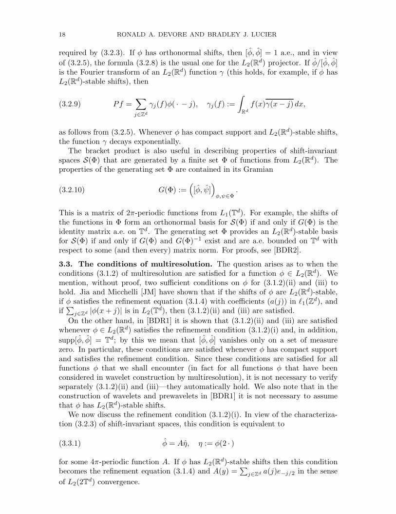
It was shown in [BDR1] that one can construct generators for the wavelet spaceW even when (3.1.2)(iv) does not hold. For example, this condition can be replaced
by the assumption that supp φ = Rd. We also note that if [φ, φ] is nonzero a.e., thenwe can always find a generator φ∗ for S with orthonormal shifts, so the condition(3.1.2)(ii) is satisfied for this generator (and the other conditions of multiresolutionremain the same). However, the generator φ∗ does not satisfy the same refinementequation as φ (for example, the refinement equation for φ∗ may be an infinite sumeven if the equation for φ is a finite sum) and φ∗ may not have compact supporteven if φ has compact support, so the construction that gives φ∗ is not completelysatisfactory. Furthermore, we would like to describe the wavelets and prewaveletsdirectly in terms of the original φ. This is especially the case when φ does nothave L2(R
d)-stable shifts, since then we can say nothing about the decay of φ∗even when φ has compact support. In the remainder of this presentation, we shallassume that φ has L2(R
d)-stable shifts.
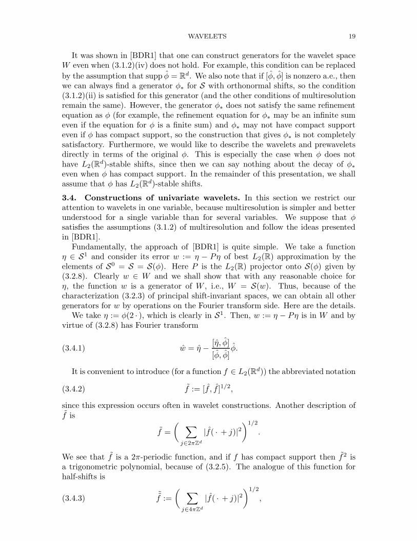
3.4. Constructions of univariate wavelets. In this section we restrict ourattention to wavelets in one variable, because multiresolution is simpler and betterunderstood for a single variable than for several variables. We suppose that φsatisfies the assumptions (3.1.2) of multiresolution and follow the ideas presentedin [BDR1].
Fundamentally, the approach of [BDR1] is quite simple. We take a functionη ∈ S1 and consider its error w := η − Pη of best L2(R) approximation by theelements of S0 = S = S(φ). Here P is the L2(R) projector onto S(φ) given by(3.2.8). Clearly w ∈ W and we shall show that with any reasonable choice forη, the function w is a generator of W , i.e., W = S(w). Thus, because of thecharacterization (3.2.3) of principal shift-invariant spaces, we can obtain all othergenerators for w by operations on the Fourier transform side. Here are the details.
We take η := φ(2 · ), which is clearly in S1. Then, w := η − Pη is in W and byvirtue of (3.2.8) has Fourier transform
(3.4.1) w = η − [η, φ]
[φ, φ]φ.
It is convenient to introduce (for a function f ∈ L2(Rd)) the abbreviated notation
(3.4.2) f := [f , f ]1/2,
since this expression occurs often in wavelet constructions. Another description off is
f =
( ∑
j∈2πZd
|f( · + j)|2)1/2
.
We see that f is a 2π-periodic function, and if f has compact support then f2 isa trigonometric polynomial, because of (3.2.5). The analogue of this function forhalf-shifts is
(3.4.3)˜f :=
( ∑
j∈4πZd
|f( · + j)|2)1/2
,
20 RONALD A. DEVORE AND BRADLEY J. LUCIER
which is now a 4π-periodic function. In particular f has orthonormal half-shifts if
and only if˜f = 2−d/2 a.e., and L2(R
d)-stable half-shifts if and only if C1 ≤ ˜f ≤ C2,
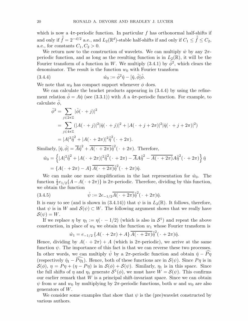
a.e., for constants C1, C2 > 0.We return now to the construction of wavelets. We can multiply w by any 2π-
periodic function, and as long as the resulting function is in L2(R), it will be the
Fourier transform of a function in W . We multiply (3.4.1) by φ2, which clears thedenominator. The result is the function w0 with Fourier transform
(3.4.4) w0 := φ2η − [η, φ]φ.
We note that w0 has compact support whenever φ does.We can calculate the bracket products appearing in (3.4.4) by using the refine-
ment relation φ = Aη (see (3.3.1)) with A a 4π-periodic function. For example, to
calculate φ,
φ2 =∑
j∈2πZ
|φ( · + j)|2
=∑
j∈4πZ
(|A( · + j)|2|η( · + j)|2 + |A( · + j + 2π)|2|η( · + j + 2π)|2)
= |A|2 ˜η2 + |A( · + 2π)|2 ˜η2( · + 2π).
Similarly, [η, φ] = A˜η2+ A( · + 2π)˜η
2( · + 2π). Therefore,
w0 =|A|2 ˜η2 + |A( · + 2π)|2 ˜η2( · + 2π)− AA˜η
2 − A( · + 2π)A˜η2( · + 2π)
η
= A( · + 2π)−AA( · + 2π)˜η2( · + 2π)η.
We can make one more simplification in the last representation for w0. Thefunction 1
2e1/2A−A( · +2π) is 2π-periodic. Therefore, dividing by this function,we obtain the function
(3.4.5) ψ := 2e−1/2A( · + 2π)˜η2( · + 2π)η.
It is easy to see (and is shown in (3.4.14)) that ψ is in L2(R). It follows, therefore,that ψ is in W and S(ψ) ⊂W . The following argument shows that we really haveS(ψ) =W .
If we replace η by η1 := η( · − 1/2) (which is also in S1) and repeat the aboveconstruction, in place of w0 we obtain the function w1 whose Fourier transform is
w1 = e−1/2 A( · + 2π) + AA( · + 2π)˜η2( · + 2π)η.
Hence, dividing by A( · + 2π) + A (which is 2π-periodic), we arrive at the samefunction ψ. The importance of this fact is that we can reverse these two processes.
In other words, we can multiply ψ by a 2π-periodic function and obtain η − P η
(respectively η1 − P η1). Hence, both of these functions are in S(ψ). Since Pη is inS(φ), η = Pη + (η − Pη) is in S(φ) + S(ψ). Similarly, η1 is in this space. Sincethe full shifts of η and η1 generate S1(φ), we must have W = S(ψ). This confirmsour earlier remark that W is a principal shift-invariant space. Since we can obtainψ from w and w0 by multiplying by 2π-periodic functions, both w and w0 are alsogenerators of W .
We consider some examples that show that ψ is the (pre)wavelet constructed byvarious authors.
WAVELETS 21
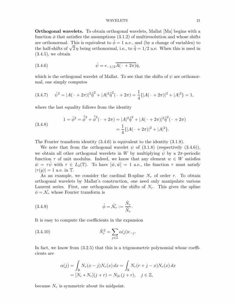
Orthogonal wavelets. To obtain orthogonal wavelets, Mallat [Ma] begins with afunction φ that satisfies the assumptions (3.1.2) of multiresolution and whose shifts
are orthonormal. This is equivalent to φ = 1 a.e., and (by a change of variables) to
the half-shifts of√2 η being orthonormal, i.e., to ˜η = 1/2 a.e. When this is used in
(3.4.5), we obtain
(3.4.6) ψ = e−1/2A( · + 2π)η,
which is the orthogonal wavelet of Mallat. To see that the shifts of ψ are orthonor-mal, one simply computes
(3.4.7) ψ2 = |A( · + 2π)|2 ˜η2 + |A|2 ˜η2( · + 2π) =1
4|A( · + 2π)|2 + |A|2 = 1,
where the last equality follows from the identity
(3.4.8)1 = φ2 =
˜φ2+
˜φ2( · + 2π) = |A|2 ˜η2 + |A( · + 2π)|2 ˜η2( · + 2π)
=1
4|A( · + 2π)|2 + |A|2.
The Fourier transform identity (3.4.6) is equivalent to the identity (3.1.8).We note that from the orthogonal wavelet ψ of (3.1.8) (respectively (3.4.6)),
we obtain all other orthogonal wavelets in W by multiplying ψ by a 2π-periodicfunction τ of unit modulus. Indeed, we know that any element w ∈ W satisfiesw = τ ψ with τ ∈ L2(T). To have [w, w] = 1 a.e., the function τ must satisfy|τ(y)| = 1 a.e. in T.
As an example, we consider the cardinal B-spline Nr of order r. To obtainorthogonal wavelets by Mallat’s construction, one need only manipulate variousLaurent series. First, one orthogonalizes the shifts of Nr. This gives the splineφ = Nr whose Fourier transform is
(3.4.9) φ = Nr :=Nr
Nr.
It is easy to compute the coefficients in the expansion
(3.4.10) N2r =
∑
j∈Z
α(j)e−j .
In fact, we know from (3.2.5) that this is a trigonometric polynomial whose coeffi-cients are
α(j) =
∫
R
Nr(x− j)Nr(x) dx =
∫
R
Nr(r + j − x)Nr(x) dx
= [Nr ∗Nr](j + r) = N2r(j + r), j ∈ Z,
because Nr is symmetric about its midpoint.
22 RONALD A. DEVORE AND BRADLEY J. LUCIER
The polynomial ρ2r(z) := zr∑j∈Z
α(j)z−j is the Euler-Frobenius polynomial of
order 2r, which plays a prominent role in cardinal spline interpolation (see [Sch1]).It is well known that ρ2r has no zeros on |z| = 1. Hence, the reciprocal 1/ρ2r isanalytic in a nontrivial annulus that contains the unit circle in its interior. Onecan easily find the coefficients of reciprocals and square roots of Laurent series
inductively. By finding the coefficients of ρ−1/22r , we obtain the coefficients β(j)
appearing in the expansion
(3.4.11) φ(x) = Nr(x) =∑
j∈Z
β(j)Nr(x− j).
Because ρ2r has no zeros on |z| = 1, we conclude that the coefficients β(j) decreaseexponentially. The spline Nr together with its shifts form an orthonormal basis forthe cardinal spline space S(Nr). They are sometimes referred to as the Franklinbasis for S(Nr).
Now that we have the spline φ := Nr in hand, we can obtain the spline waveletψ = N ∗
r of Battle-Lemarie [Ba] from formula (3.1.8). For this, we need to findthe refinement equation for φ. We begin with the refinement equation (3.1.5) for
the B-spline Nr, which we write in terms of Fourier transforms as Nr = A0η0with η0 := Nr(2 · ) and A0 = 2−r+1
∑rj=0
(rj
)e−j/2 a 4π-periodic trigonometric
polynomial. It follows that
(3.4.12) φ = Aη, η := Nr(2 · ), A(y) =φ(y)
12 φ(y/2)
= Nr(y/2)N−1r (y)A0(y).
In terms of the B-spline Nr, this gives
(3.4.13) ψ(y) = e−1/2(y)A(y + 2π)η(y) =1
2e−1/2(y)A(y + 2π)N−1
r (y/2)Nr(y/2).
In other words, to find the orthogonal spline wavelet ψ of (3.4.13), we need to
multiply out the various Laurent expansions making up A( · + 2π)N−1r ( · /2). This
gives the coefficients γ(j), j ∈ Z, in the representation
ψ(x) =∑
j∈Z
γ(j)Nr(2x− j).
We emphasize that each of the Laurent series converges in an annulus containingthe unit circle. This means that the coefficients γ(j) converge exponentially to zerowhen j → ±∞.
Prewavelets. For the construction of prewavelets, we do not assume that theshifts of φ are orthonormal, but only that they are L2(R)-stable, i.e., we assume(3.1.2)(iv). Then, it is easy to see that the function ψ defined by (3.4.5) is aprewavelet. Indeed, we already know that ψ is a generator for W and it is enoughto check that it has L2(R)-stable shifts. For this, we compute
(3.4.14)ψ2
4= |A( · + 2π)|2 ˜η4( · + 2π)˜η
2+ |A|2 ˜η4 ˜η2( · + 2π).
WAVELETS 23
Since the shifts of φ are L2(R)-stable, so are the half-shifts of η. This means that
C1 ≤ ˜η ≤ C2 for constants C1, C2 > 0. Moreover, the formula
φ2 = |A|2 ˜η2 + |A( · + 2π)|2 ˜η2( · + 2π)
shows that C1 ≤ |A|2 + |A( · + 2π)|2 ≤ C2, again for positive constants C1, C2.
Combining this information with (3.4.14) shows that ψ is bounded above and belowby positive constants, so that ψ has L2(R)-stable shifts. This also shows thatψ is in L2(R). The prewavelet ψ was introduced by Chui and Wang [CW] andindependently by Micchelli [M].
We can also find a direct representation for ψ in terms of the shifts of φ(2 · ).For this we need the Fourier coefficients µ(j) (of e−j/2) for the 4π-periodic function
2A˜η:
µ(j) :=1
4π
∫ 2π
−2π
2A˜η2ej/2 =
1
4π
∫
R
2φηej/2 =
∫
R
φη( ·+j/2) =∫
R
φ(x)φ(2x+j) dx.
Using this in (3.4.5), we find that
(3.4.15) ψ =∑
j∈Z
(−1)j+1µ(j − 1)φ(2 · − j), µ(j) :=
∫
R
φ(x)φ(2x+ j) dx.
If φ has compact support, then clearly ψ also has compact support. Chui andWang [CW1] posed the interesting question whether ψ has the smallest supportamong all the elements in W , to which they gave the following answer. We assumethat A is a polynomial, i.e., that φ satisfies a finite refinement equation. Next, wenote that because W ⊂ S1, any w ∈W is represented as
(3.4.16) w(y) = e−1/2(y)B(y+ 2π)η(y)
with B of period 4π. If B =∑M
j=m b(j)e−j/2 is a Laurent polynomial with
b(m)b(M) 6= 0, then w has compact support, and we define the length of B tobe M − m. We know that there are nonzero polynomials B that satisfy (3.4.16)
for some w because ˜η2is a polynomial (since η has compact support) and (3.4.5)
implies that for B0 := A˜η2, w is the prewavelet ψ ∈W .
B0 may not have minimal length among all such polynomials, however, becauseit may be possible to cancel certain symmetric factors from B0. To see this, we writeB0(y) = eM (y/2)P (e−iy/2) with P an algebraic polynomial, and we let Q(z2) :=∏λ(z−λ), with the product taken over all λ with λ and −λ both zeros of P . Then,
the factorization P (z) = Q(z2)P∗(z) gives the factorization B0(y) = τ(y)B∗(y)with τ a trigonometric polynomial of period 2π that does not vanish. Therefore,the function ψ∗ with Fourier transform
(3.4.17) ψ∗(y) = e−1/2(y)B∗(y + 2π)η(y), B∗(y) := τ−1(y)B0(y),
is inW and has smaller length than B0. A simple argument (which we do not give)shows that B∗ has smallest length. For most prewavelets of interest, B∗ = B0.
24 RONALD A. DEVORE AND BRADLEY J. LUCIER
0 1
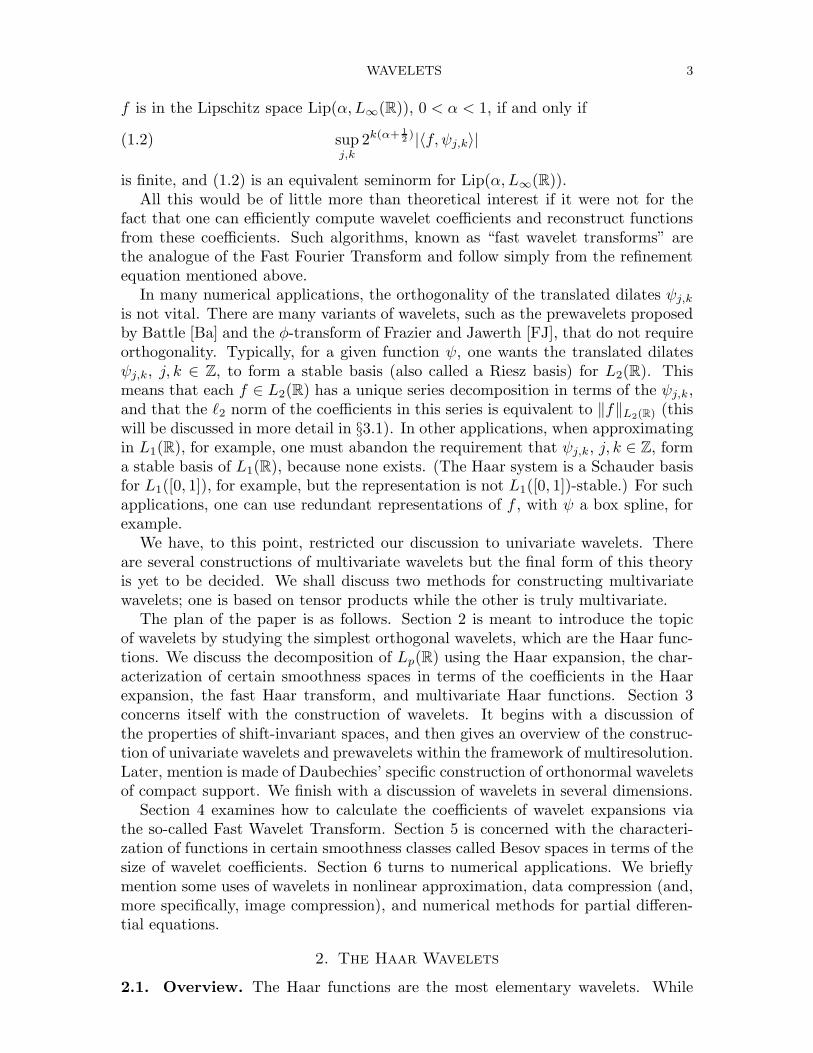
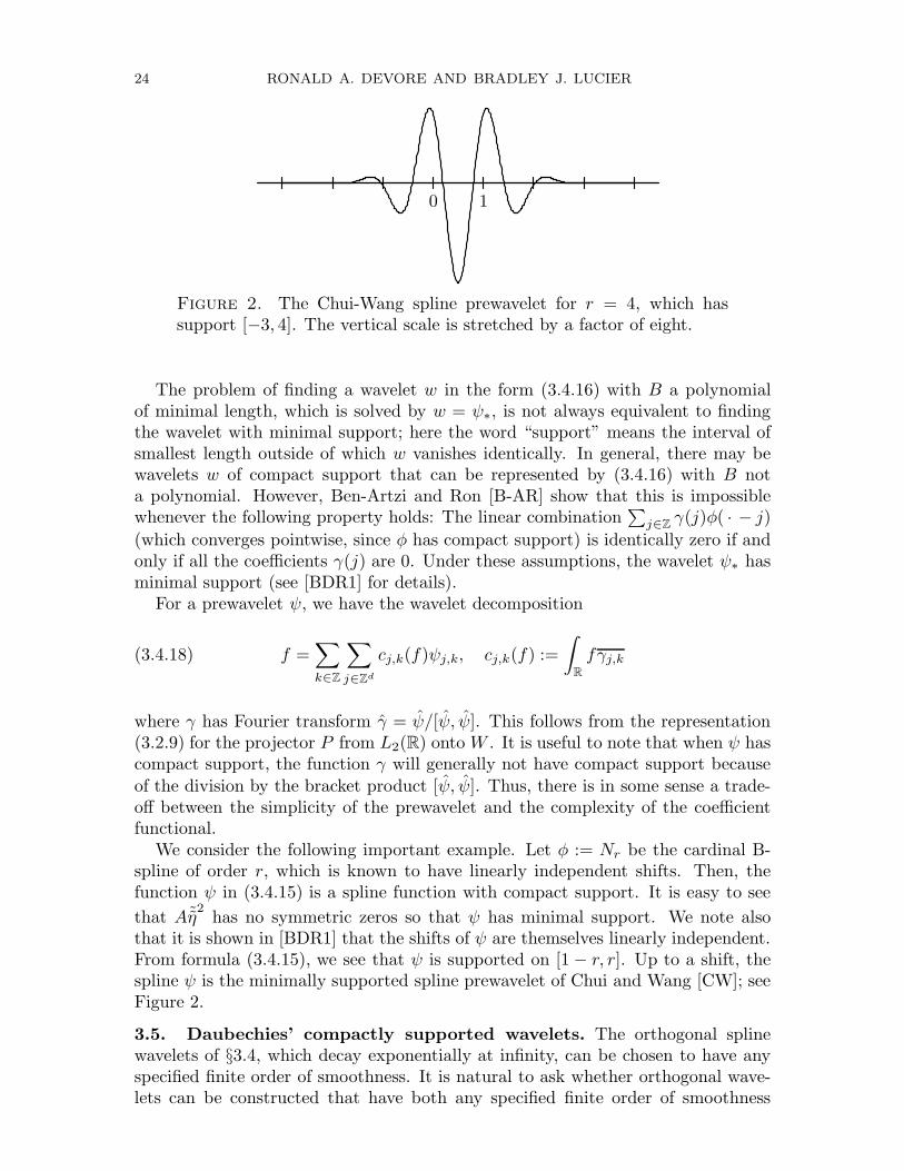
Figure 2. The Chui-Wang spline prewavelet for r = 4, which hassupport [−3, 4]. The vertical scale is stretched by a factor of eight.
The problem of finding a wavelet w in the form (3.4.16) with B a polynomialof minimal length, which is solved by w = ψ∗, is not always equivalent to findingthe wavelet with minimal support; here the word “support” means the interval ofsmallest length outside of which w vanishes identically. In general, there may bewavelets w of compact support that can be represented by (3.4.16) with B nota polynomial. However, Ben-Artzi and Ron [B-AR] show that this is impossiblewhenever the following property holds: The linear combination
∑j∈Z
γ(j)φ( · − j)
(which converges pointwise, since φ has compact support) is identically zero if andonly if all the coefficients γ(j) are 0. Under these assumptions, the wavelet ψ∗ hasminimal support (see [BDR1] for details).
For a prewavelet ψ, we have the wavelet decomposition
(3.4.18) f =∑
k∈Z
∑
j∈Zd
cj,k(f)ψj,k, cj,k(f) :=
∫
R
fγj,k
where γ has Fourier transform γ = ψ/[ψ, ψ]. This follows from the representation(3.2.9) for the projector P from L2(R) ontoW . It is useful to note that when ψ hascompact support, the function γ will generally not have compact support becauseof the division by the bracket product [ψ, ψ]. Thus, there is in some sense a trade-off between the simplicity of the prewavelet and the complexity of the coefficientfunctional.
We consider the following important example. Let φ := Nr be the cardinal B-spline of order r, which is known to have linearly independent shifts. Then, thefunction ψ in (3.4.15) is a spline function with compact support. It is easy to see
that A˜η2has no symmetric zeros so that ψ has minimal support. We note also
that it is shown in [BDR1] that the shifts of ψ are themselves linearly independent.From formula (3.4.15), we see that ψ is supported on [1− r, r]. Up to a shift, thespline ψ is the minimally supported spline prewavelet of Chui and Wang [CW]; seeFigure 2.
3.5. Daubechies’ compactly supported wavelets. The orthogonal splinewavelets of §3.4, which decay exponentially at infinity, can be chosen to have anyspecified finite order of smoothness. It is natural to ask whether orthogonal wave-lets can be constructed that have both any specified finite order of smoothness
WAVELETS 25
and compact support. A celebrated construction of Daubechies [Da] leads to suchwavelets, which are frequently used in numerical applications. Space prohibits usfrom giving all the details of Daubechies’ construction, but the following discussionwill outline the basic ideas.
To construct a compactly supported wavelet with a prescribed smoothness or-der r and compact support, one finds a special finite sequence (a(j)) such thatthe refinement equation (3.1.4) has a solution φ ∈ Cr with orthogonal shifts. Theorthogonal wavelet ψ of (3.4.5) will then obviously have compact support and thesame smoothness. Before we begin, it is necessary to understand which propertiesof the sequence (a(j)) guarantee the existence of a function φ with the desiredproperties, i.e., we need to understand the nature of solutions to the refinementequation (3.1.4). This has been studied in another context, namely, in subdivi-sion algorithms for computer aided geometric design (see, for example, the paperof Cavaretta, Dahmen, and Micchelli [CDM] for a discussion of subdivision). Aswas pointed out by Dahmen and Micchelli [DM], it is possible to derive part ofDaubechies’ construction from the subdivision approach. However, we shall de-scribe Daubechies’ original construction.
Let r be a nonnegative integer that corresponds to the desired order of smooth-ness, and let (a(j)) with a(j) = 0, |j| > m, and a(m) 6= 0, be the sequence of therefinement equation (3.1.4) for the function φ we want to construct. The sequence(a(j)) and the Fourier transform of φ are related by
(3.5.1) φ(y) = A(y/2)φ(y/2), A(y) :=1
2
m∑
j=−m
a(j)e−ijy.
Here we use a slightly different normalization for the refinement function (A(y) =12A(2y)). If φ is continuous at 0 and φ(0) = 1, we can, at least in a formal sense,
write
(3.5.2) φ(y) = limk→∞
Ak(y)
where
(3.5.3) Ak(y) :=k∏
j=1
A(y/2j).
We note that A∗k(y) := Ak(2
ky) is a trigonometric polynomial of degree (2k −1)m. The key to Daubechies’ construction is to impose conditions on A (which aretherefore conditions on the sequence (a(j))) that not only make (3.5.2) rigorous butalso guarantee that the function φ defined by (3.5.2) has the desired smoothnessand has orthonormal shifts.
We first note that if the shifts of φ are orthonormal then, as was shown in (3.4.8),
(3.5.4) |A(y)|2 + |A(y + π)|2 = 1, y ∈ T.
The converse to this is almost true. Namely, Daubechies’ construction shows that(3.5.4) together with some mild assumptions (related to the convergence in (3.5.3))
26 RONALD A. DEVORE AND BRADLEY J. LUCIER
imply the orthonormality of the shifts of φ. For this, the following identities, whichfollow from (3.5.4) by induction, are useful:
(3.5.5)2k−1∑
j=0
|A∗k(y + j2−k2π)|2 = 1, k = 1, 2 . . . .
We next want to see what properties of A guarantee smoothness for φ. Thestarting point is the following observation. If
∫Rφ(x) dx 6= 0, then integrating the
refinement equation (3.1.4) gives∑
j∈Za(j) = 2. Hence, A(0) = 1 and A(π) = 0.
We can therefore write
(3.5.6) A(y) = (1 + eiy)Nα(y), ‖α‖L∞(T) = 2−θ, α(0) = 2−N ,
for a suitable integer N > 0, a real number θ, and a function α.By carefully estimating the partial products Ak, it can be shown that whenever
A satisfies (3.5.6) for some θ > 1/2, the product (3.5.2) converges to a functionin L2(R) that decays like |x|−θ as |x| → ∞. The limit function is the Fouriertransform of the solution φ to the refinement equation (3.5.1). We see that thelarger we can make θ in (3.5.6), the smoother φ is. For example, if θ > r + 1, thenφ is in Cr.
What is the role of the integer N in (3.5.6)? Practically, one must increaseN to find a function α(y) that satisfies (3.5.6) for large θ. In addition, the localapproximation properties of the spaces Sk(φ) are determined by N ; see §5.
Once it is shown that there is a function φ that satisfies the refinement equationfor the given sequence (a(j)), it remains to show that φ has compact support andorthonormal shifts. Here the arguments have the same character as those usedto analyze subdivision algorithms for the graphical display of curves and surfaces.Assume that A satisfies (3.5.4) and (3.5.6) for some θ > 1/2 and let χ denote thecharacteristic function of [−1/2, 1/2]. Then χ(y) = (sin y/2)/(y/2). We define φkto be the function whose Fourier transform is φk(y) := Ak(y)χ(2
−ky). It can thenbe shown that
(3.5.7)
∫
R
|φ(y)− φk(y)|2 dy → 0, k → ∞.
If A∗k =
∑j a
∗(j, k)e−j , then∑j a
∗(j, k)χ(x−j) has Fourier transform A∗k(y)χ(y)
and φk(y) = A∗k(2
−ky)χ(2−ky). Therefore,
(3.5.8) φk(x) =∑
j∈Z
a∗(j, k)2kχ(2kx− j).
Since the coefficients a∗(j, k) of A∗k are 0 for |j| > (2k − 1)m, we obtain that
φk is supported in [−m,m]. Letting k → ∞, we obtain from (3.5.7) that φ isalso supported on [−m,m]. From (3.5.8), (3.5.5), and the orthonormality of thefunctions 2k/2χ(2k· − j), j ∈ Z, we have
∫
R
φk(x)φk(x− ℓ) dx = 2k∑
µ−ν=2kℓ
a∗(µ, k)a∗(ν, k) = δ(ℓ), ℓ ∈ Z.
WAVELETS 27
Here the last equality follows by expanding the identity (3.5.5). Letting k → ∞,we obtain that φ( · − j)j∈Z is an orthonormal system.
The above outline shows that a Cr, compactly supported function φ with or-thonormal shifts exists if (3.5.4) and (3.5.6) hold for a sequence (a(j)) and twonumbers N and θ > r + 1. The following arguments show that such sequencesexist.
We look for an A of the form (3.5.6) with α a trigonometric polynomial with
real coefficients. Then, |α(y)|2 = α(y)α(y) = α(y)α(−y) is an even trigonometricpolynomial, and
|α(y)|2 = T (cos y) = T (1− 2 sin2 y/2) = R(sin2 y/2)
with R an algebraic polynomial. The identity (3.5.4) now becomes
(cos2 y/2)NR(sin2 y/2) + (sin2 y/2)NR(cos2 y/2) = 2−2N .
With t := sin2 y/2, we have
(3.5.9) (1− t)NR(t) + tNR(1− t) = 2−2N .
Therefore, to find A, we must find an algebraic polynomial R that satisfies(3.5.9). It is easy to see that the degree of R must be at least N − 1. We can findR of this degree by writing R in the Bernstein form
R(t) =N−1∑
k=0
λk
(N − 1
k
)tk(1− t)N−k−1.
Then, (3.5.9) becomes
(3.5.10)
(1− t)NN−1∑
k=0
λk
(N − 1
k
)tk(1− t)N−k−1 + tN
N−1∑
k=0
λk
(N − 1
k
)(1− t)ktN−k−1
= 2−2N = 2−2N2N−1∑
k=0
(2N − 1
k
)tk(1− t)2N−1−k.
We see that
λk := 2−2N
(2N−1k
)(N−1k
) , k = 0, 1, . . . , N − 1,
satisfies (3.5.10), and we denote the polynomial with these coefficients by RN .It is important to observe that RN (t) is nonnegative for 0 ≤ t ≤ 1, be-
cause we wish to show that there is a trigonometric polynomials α(y) such thatRN (sin
2 y/2) = |α(y)|2, i.e., we somehow have to take a “square root” of RN . Forthis, we use the classical theorem of Fejer-Riesz (see for example Karlin and Studden[KS, pg. 185]) that says that if R is nonnegative on [0, 1], then R(sin2 y/2) = |α(y)|2
28 RONALD A. DEVORE AND BRADLEY J. LUCIER
for some trigonometric polynomial α with real coefficients and of the same degreeas R. We let αN be the trigonometric polynomial corresponding to RN .
We now set AN (y) := (1+eiy)NαN (y) and note that AN satisfies (3.5.4) becauseRN satisfies (3.5.9). Therefore, the function φ defined via the limit process (3.5.2)has compact support and orthonormal shifts. The corresponding orthogonal waveletψ =: D2N defined by (3.1.8) for the refinement coefficients (a(j)) is an orthogonalwavelet with compact support. It is easy to show that D2N is supported in [−(N −1), N ].
The question now is what is the smoothness of D2N . Here the matter can becomesomewhat technical (see Daubechies [Da] and Meyer [Me1]). However, the following“poor man’s” argument based on Stirling’s formula at least shows that given anyinteger r, if we choose N sufficiently large, the orthogonal wavelet D2N will havesmoothness Cr.
Because the Bernstein coefficients of RN are monotone, it follows that RN isincreasing on [0, 1]. Therefore, max0≤t≤1RN (t) = RN (1) = λN−1 = 2−2N
(2N−1N
).
Therefore, ‖αN‖2L∞(T) is bounded by
2−2N
(2N − 1
N
)≤ 2−2N
√2π(2N − 1)(2N − 1)2N−1e−(2N−1)
√2πNNNe−N
√2π(N − 1)(N − 1)N−1e−(N−1)
≤ C0N−1/2,
by Stirling’s formula. We see that given any value of θ > 0, we can choose Nlarge enough so that (3.5.6) is satisfied for that θ, and the function φ satisfies
|φ(x)| ≤ C(1 + |x|)−θ. Hence, for any r < θ − 1, φ, and hence D2N , is in Cr.
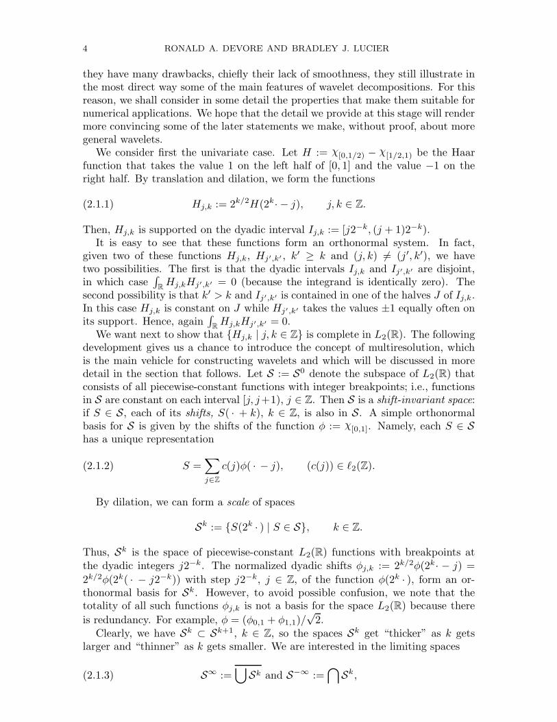
For N = 1, the Daubechies construction gives φ = χ[0,1] and D2 is the Haarfunction. For N = 2, the polynomial R2(t) = (1 + 2t)/16 and
A2(y) = (1 + eiy)2(
√3 + 1
8−
√3− 1
8e−iy) = (1 + eiy)2α2(y).
Then α2(y) satisfies |α2(y)| ≤√3/4 < 2−1. Therefore, the function φ and the
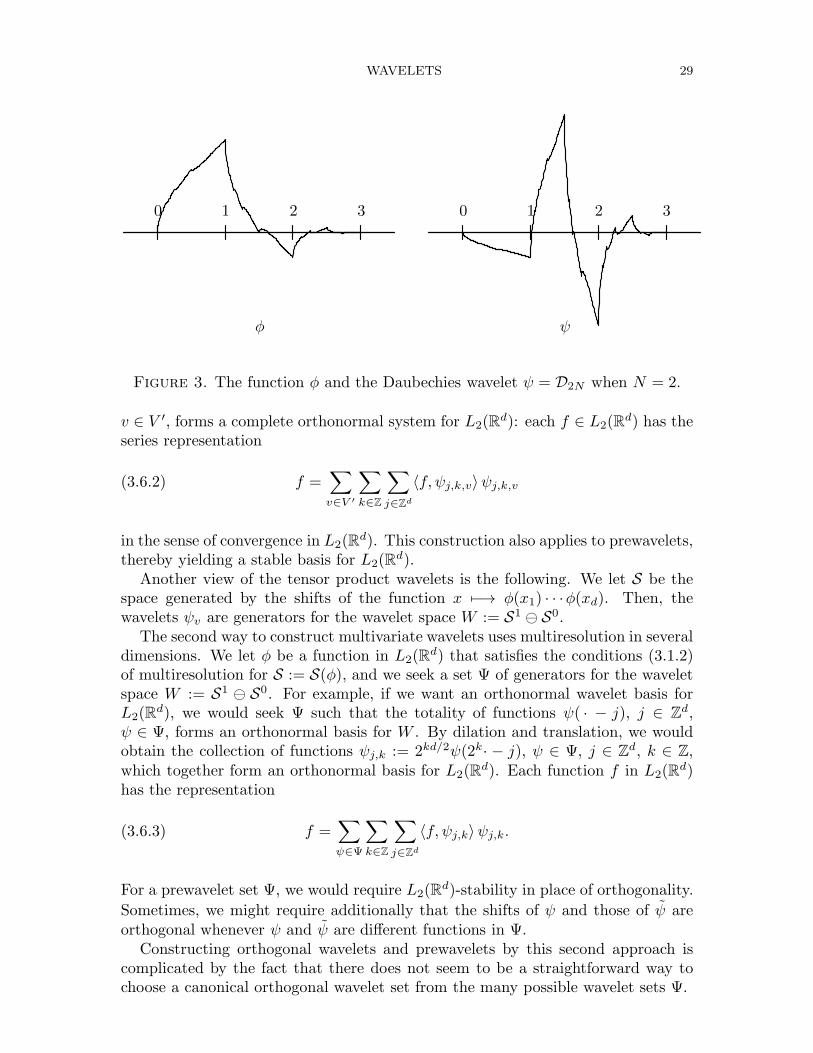
wavelet D4 := ψ corresponding to this choice is continuous. (See Figure 3 for agraph of φ and ψ.) A finer argument shows that D4 is in Lip(.55, L∞(R)). Thereader can consult Daubechies [Da] for a table of the refinement coefficients of D2N
for other values of N and a more precise discussion of the smoothness of D2N inL∞(R).
3.6. Multivariate wavelets. There are two approaches to the construction ofmultivariate wavelets for L2(R
d). The first, the tensor product approach, we nowbriefly describe. In this section, V will denote the set of vertices of the cube [0, 1]d
and V ′ := V \0. Let φ be a univariate function satisfying the conditions (3.1.2) ofmultiresolution and let ψ be an orthogonal wavelet obtained from φ. For φ0 := φ,φ1 := ψ, the collection Ψ of functions
(3.6.1) ψv(x1, . . . , xd) := φv1(x1) · · ·φvd(xd), v ∈ V ′,
generates, by dilation and translation, a complete orthonormal system for L2(Rd).
More precisely, the collection of functions ψj,k,v := 2kd/2ψv(2k· − j), j ∈ Zd, k ∈ Z,
WAVELETS 29
0 1 2 3
ψ
0 1 2 3
φ
Figure 3. The function φ and the Daubechies wavelet ψ = D2N when N = 2.
v ∈ V ′, forms a complete orthonormal system for L2(Rd): each f ∈ L2(R
d) has theseries representation
(3.6.2) f =∑
v∈V ′
∑
k∈Z
∑
j∈Zd
〈f, ψj,k,v〉ψj,k,v
in the sense of convergence in L2(Rd). This construction also applies to prewavelets,
thereby yielding a stable basis for L2(Rd).
Another view of the tensor product wavelets is the following. We let S be thespace generated by the shifts of the function x 7−→ φ(x1) · · ·φ(xd). Then, thewavelets ψv are generators for the wavelet space W := S1 ⊖ S0.
The second way to construct multivariate wavelets uses multiresolution in severaldimensions. We let φ be a function in L2(R
d) that satisfies the conditions (3.1.2)of multiresolution for S := S(φ), and we seek a set Ψ of generators for the waveletspace W := S1 ⊖ S0. For example, if we want an orthonormal wavelet basis forL2(R
d), we would seek Ψ such that the totality of functions ψ( · − j), j ∈ Zd,ψ ∈ Ψ, forms an orthonormal basis for W . By dilation and translation, we wouldobtain the collection of functions ψj,k := 2kd/2ψ(2k· − j), ψ ∈ Ψ, j ∈ Zd, k ∈ Z,which together form an orthonormal basis for L2(R
d). Each function f in L2(Rd)
has the representation
(3.6.3) f =∑
ψ∈Ψ
∑
k∈Z
∑
j∈Zd
〈f, ψj,k〉ψj,k.
For a prewavelet set Ψ, we would require L2(Rd)-stability in place of orthogonality.
Sometimes, we might require additionally that the shifts of ψ and those of ψ areorthogonal whenever ψ and ψ are different functions in Ψ.
Constructing orthogonal wavelets and prewavelets by this second approach iscomplicated by the fact that there does not seem to be a straightforward way tochoose a canonical orthogonal wavelet set from the many possible wavelet sets Ψ.
30 RONALD A. DEVORE AND BRADLEY J. LUCIER
The book of Meyer [Me] contains first results on the construction of multivariatewavelet sets by the second approach. This was expanded upon in the paper of Jiaand Micchelli [JM]. These treatments are not always constructive; for example, thelatter paper employs in some contexts the Quillen-Suslin theorem from commutativealgebra. Several papers [RS], [RS1], [CSW], and [LM] treat special cases, such asthe construction of orthogonal wavelet and prewavelet sets when φ is taken to be abox spline. The paper of Riemenschneider and Shen [RS] is particularly important,since it gives a constructive approach that applies in two and three dimensions toa wide class of functions φ.
We shall follow the approach of [BDR1], which is based on the structure of shift-invariant spaces. This approach immediately gives a generating set for W , whichcan then be exploited to find orthogonal wavelet and prewavelet sets. de Boor,DeVore, and Ron start with a function φ that satisfies the refinement relation(3.1.2)(i) and whose Fourier transform satisfies supp φ = Rd. It is not necessary inthis approach to assume (3.1.2) (ii) and (iii)—they follow automatically. It is alsonot necessary to assume (3.1.2) (iv). In particular, this approach applies to anycompactly supported φ. To simplify our discussion, we shall assume in addition to(3.1.2)(i) that φ has compact support and that the shifts of φ are L2(R
d)-stable;we refer the reader to [BDR1] for a discussion of the more general theory.
The usual starting point for the construction of multivariate wavelets is the factthat the dilated space S1 of S := S(φ) is generated by the half-shifts of η := φ(2 · ),and therefore also by the full shifts of the functions ηv := η( · − v/2), v ∈ V .
The assumption that supp φ = Rd is important because it implies that the setΦ := φv := φ(x − v/2) | v ∈ V is also a generating set for S1, i.e., S1 = S(Φ).Φ is more useful than ηv | v ∈ V as a generating set because Φ contains afunction that is in S0, namely φ. In analogy with the univariate construction, wesee that with P the L2(R
d) projector onto S, the functions φv − Pφv, v ∈ V ′,form a generating set for W . From (3.2.8), we calculate the Fourier transforms of
these functions and multiply them by [φ, φ] to obtain the functions wv, with Fouriertransform
(3.6.4) wv := [φ, φ]φv − [φv, φ]φ, v ∈ V ′.
The set W := wv | v ∈ V ′ is another generating set for W . We note that becausewe assume φ has compact support, the two bracket products appearing in (3.6.4) aretrigonometric polynomials, and hence the functions wv also have compact support.
The set TW, with T = (τv,v′)v,v′∈V ′ a matrix of 2π-periodic functions, is anothergenerating set for W if det(T ) 6= 0 a.e.
It is easy to find an orthogonal wavelet set by this approach. Because thefunctions in W have compact support, the Gramian matrix ([wv, wv′ ])v,v′∈V ′ hastrigonometric polynomials as its entries. Since this matrix is symmetric and pos-itive semidefinite, its determinant is nonzero a.e. We can use Gauss elimination(Cholesky factorization) without division or pivoting to diagonalize G(W). Thatis, we can find a (symmetric) matrix T = (τv,v′)v,v′∈V ′ of trigonometric polynomi-als such that W∗ := TW has Gramian G(TW∗) = TG(W)T ∗ that is a diagonalmatrix with trigonometric polynomial entries. If w∗
v are the functions in W∗, thenthe functions w∗∗
v with Fourier transforms w∗∗v := w∗
v/[w∗v, w
∗v]
1/2, v ∈ V ′, have
WAVELETS 31
shifts that form an orthonormal basis for W . Indeed,
[w∗∗v , w
∗∗v′ ] =
[w∗v, w
∗v′ ]
[w∗v , w
∗v]
1/2[w∗v′ , w
∗v′ ]
1/2,
which shows that the new set of generators W∗∗ has the identity matrix as itsGramian.
The disadvantage of the orthogonal wavelet set W∗∗ is that usually we can saynothing about the decay of the functions w∗∗
v , since the above construction mayinvolve division by trigonometric polynomials that have zeros. However, when φhas L2(R
d)-stable half-shifts, the above construction can be modified to give anorthogonal wavelet set whose elements decay exponentially (see [BDR1]).
While the assumption that the half-shifts of φ are L2(Rd)-stable is often not
realistic, we shall assume it a little longer in order to introduce some new ideasthat can later be modified to drop the stability assumption. Under the half-shift
stability assumption, we have that˜φ is a trigonometric polynomial of period 4π that
has no zeros. Therefore, φ∗ := φ/˜φ serves to define an L2(R
d) function in S1(φ)that decays exponentially and has orthogonal half-shifts. Moreover, the function
w with Fourier transform w := φ/˜φ2is also in S1(φ) and decays exponentially.
Therefore, with [ · , · ]1/2 the bracket product for half-shifts (which is defined as in
(3.2.4) except that the sum is taken over 4πZd), we have
(3.6.5) [φ, w]1/2 = [φ∗, φ∗]1/2 = 1 a.e.
The Fourier coefficients (with respect to the e−j/2, j ∈ Zd) of [φ, w]1/2 are theinner products of φ with half-shifts of w. Hence, all nontrivial half-shifts of w areorthogonal to φ. This means that the functions in W0 := w( · + v/2) | v ∈ V ′are all in W . It is easy to see that they generate W , that is, W = S(W0).
Thus, in the special case we are considering, W is generated by the nontrivialhalf-shifts of a single function w. It is natural to ask whether this holds in general(i.e., when we do not assume stability of half-shifts). To see that this is indeed true,we modify the argument in (3.6.5). If we multiply w by the 2π-periodic function∏λ∈2πV
˜φ( · +λ)2, the result is a compactly supported function w∗ ∈ L2(R
d), withFourier transform
(3.6.6) w∗ := φ∏
λ∈2πV ′
˜φ( · + λ)2.
We find that
(3.6.7) [φ, w∗]1/2 =∏
λ∈2πV
˜φ( · + λ)2.
Because the right side is 2π-periodic, we deduce that the inner product of φ withw∗( · − j/2) is zero whenever j = v + 2k with v ∈ V ′ and k ∈ Zd. Hence, thefunctions w∗( · + v/2), v ∈ V ′, are all in W and it is easy to see that they are alsoa generating set for W .
32 RONALD A. DEVORE AND BRADLEY J. LUCIER
While the nontrivial half-shifts of w∗ are a generating set for W , they havethe drawback that they usually do not provide an L2(R
d)-stable basis. The usualapproach towards constructing an L2(R
d)-stable basis for W is to begin with thegenerating set ηv | v ∈ V , η := φ(2 · ), for S1(φ). With this as a starting point,Meyer [Me, III, §6] and Jia and Micchelli [JM] have shown the existence of a set ofgenerators for W consisting of compactly supported functions whose shifts providean L2(R
d)-stable basis for W . However, their proofs are not constructive. In one,two, or three dimensions, and with an additional assumption on the symmetry ofφ, Riemenschneider and Shen [RS], [RS1] have given a constructive proof for theexistence of such a generating set, which we now describe.
We begin again with the function w := φ/˜φ2. If τ =
∑j∈Zd c(j)e−j/2 is a 4π-
periodic function whose Fourier coefficients c(j) = 0 whenever j ∈ 2Zd, then thefunction with Fourier transform τw is inW provided it is in L2(R
d). The conditionon these Fourier coefficients is equivalent to requiring that
(3.6.8)∑
v∈2πV
τ( · + v) = 0 a.e.
In particular, we can use this method to produce functions in W as follows.We assume that φ is real valued, has L2(R
d)-stable shifts, and satisfies the re-finement equation (3.3.1) for a real valued function A. This assumption on A is anew ingredient; it will be fulfilled for example if φ(−x) = φ(x). (More generally,one only needs symmetry about the center of the support of φ.) If α ∈ V ′ andvα ∈ 2πV , then we claim that the function ψα with Fourier transform
(3.6.9) ψα := 2eα/2 (A˜η2)( · + vα)η
is in W , provided eα/2(vα) = −1. Indeed, the refinement equation says that w =
η/(A˜η2). We obtain ψα from w by multiplying by τα := 2eα/2A˜η
2A( · + vα)˜η
2( · +
vα). The vertices v and v + vα (modulo 2π) contribute values in (3.6.8) that arenegatives of one another. Hence, (3.6.8) is satisfied for τα and ψα ∈ W . Thefunctions ψα have compact support when A is a polynomial and φ has compactsupport.
We are allowed to make any assignment of α 7−→ vα with eα/2(vα) = −1. To
obtain an L2(Rd)-stable basis forW , we need a special assignment with the property
that α−β (modulo 2) is assigned vα−vβ (modulo 2π). If such a special assignment
can be made, then a simple computation shows that with µ := 2A˜η2,
(3.6.10) [ψα, ψβ] =∑
v∈2πV
e(α−β)/2( · + v)µ( · + v + vα)µ( · + v + vβ) ˜η2( · + v).
For example, if the shifts of φ are orthonormal, then ˜η2= 1/2. In this case, for
α 6= β, the terms of the sum in (3.6.10) are negatives of one another for the twovalues v and v+(vα+vβ) (this is where we need to assume that a special assignmentexists), and hence the sum in (3.6.10) is 0. When α = β, this sum is
∑
v∈2πV
A2( · + v)˜η2( · + v) =
∑
v∈2πV
˜φ2( · + v) = φ2 = 1 a.e.
WAVELETS 33
Hence, the Gramian of Ψ := ψα | α ∈ V ′ is the identity matrix. We obtain inthis way an orthonormal basis for W .
If we begin with a φ that has L2(Rd)-stable shifts then a slightly more compli-
cated argument shows that the functions ψα, α ∈ V ′, are an L2(Rd)-stable basis
for W .This leaves the question of when we can make an assignment α 7−→ vα of this
special type. Such assignments are possible for d = 1, 2, 3 but not for d > 3. Forexample, when d = 2, we can make the assignments as follows:
(0, 0) 7−→ 2π(0, 0), (0, 1) 7−→ 2π(0, 1),
(1, 0) 7−→ 2π(1, 1), (1, 1) 7−→ 2π(1, 0).
The above construction will give orthogonal wavelet and prewavelet sets for boxsplines. To illustrate this, we consider briefly the following special box splines onR2. Let ∆ be the triangulation of R2 obtained from grid lines x1 = k, x2 = k, andx2 − x1 = k, k ∈ Z. Let M be the Courant element for this partition. Thus, M isthe piecewise linear function for this triangulation that takes the value 1 at (0, 0)and the value 0 at all other vertices. The Fourier transform of M is
M(y1, y2) =
(sin(y1/2)
y1/2
)(sin(y2/2)
y2/2
)(sin((y1 + y2)/2)
(y1 + y2)/2
).
By convolving M with itself, we obtain higher order box splines defined recursivelyby M1 := M and Mr := M ∗Mr−1. Then Mr is a compactly supported piecewisepolynomial (with respect to ∆) of degree 3r − 2 and smoothness C2r−2. Since
M is real, the box spline Mr satisfies the refinement identity (3.3.1) with A real.Therefore, if we take φ :=Mr and S = S(Mr), the construction of Riemenschneiderand Shen applies to give a prewavelet set Ψ consisting of three compactly supportedpiecewise polynomials for the partition ∆/2. The set Ψ provides an L2(R
d)-stablebasis for the wavelet space W .
4. Fast Wavelet Transforms
It is easy to compute the coefficients in wavelet decompositions iteratively witha technique similar to the fast Haar transform. We shall limit our discussion toDaubechies’ orthogonal wavelets with compact support in one dimension. How-ever, the ideas presented here apply equally well to other orthogonal wavelets andto prewavelets. We let φ be a real-valued, compactly-supported function with or-thonormal shifts that satisfies the conditions of multiresolution and in particularthe refinement equation (3.1.4). The function φ is real and the refinement coeffi-cients are real and finite in number. The orthogonal wavelet ψ is then obtainedfrom φ by (3.1.8).
A numerical application begins with a finite representation of a function f as awavelet sum. This is accomplished by choosing a large value of n, commensuratewith the numerical accuracy desired, and taking an approximation to f of the form
(4.1) Sn =∑
j∈Z
fjφj,n,
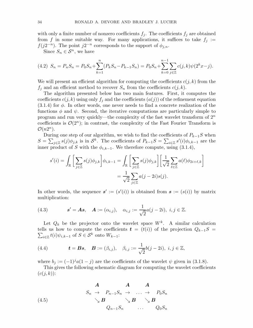
34 RONALD A. DEVORE AND BRADLEY J. LUCIER
with only a finite number of nonzero coefficients fj . The coefficients fj are obtainedfrom f in some suitable way. For many applications, it suffices to take fj :=f(j2−n). The point j2−n corresponds to the support of φj,n.
Since Sn ∈ Sn, we have
(4.2) Sn = PnSn = P0Sn+n∑
k=1
(PkSn−Pk−1Sn) = P0Sn+n−1∑
k=0
∑
j∈Z
c(j, k)ψ(2kx−j).
We will present an efficient algorithm for computing the coefficients c(j, k) from thefj and an efficient method to recover Sn from the coefficients c(j, k).
The algorithm presented below has two main features. First, it computes thecoefficients c(j, k) using only fj and the coefficients (a(j)) of the refinement equation(3.1.4) for φ. In other words, one never needs to find a concrete realization of thefunctions φ and ψ. Second, the iterative computations are particularly simple toprogram and run very quickly—the complexity of the fast wavelet transform of 2n
coefficients is O(2n); in contrast, the complexity of the Fast Fourier Transform isO(n2n).
During one step of our algorithm, we wish to find the coefficients of Pk−1S whenS =
∑j∈Z
s(j)φj,k is in Sk. The coefficients of Pk−1S =∑i∈Z
s′(i)φi,k−1 are the
inner product of S with the φi,k−1. We therefore compute, using (3.1.4),
s′(i) =
∫
R
[∑
j∈Z
s(j)φj,k
]φi,k−1 =
∫
R
[∑
j∈Z
s(j)φj,k
][1√2
∑
ℓ∈Z
a(ℓ)φ2i+ℓ,k
]
=1√2
∑
j∈Z
a(j − 2i)s(j).
In other words, the sequence s′ := (s′(i)) is obtained from s := (s(i)) by matrixmultiplication:
(4.3) s′ = As, A := (αi,j), αi,j :=1√2a(j − 2i), i, j ∈ Z.
Let Qk be the projector onto the wavelet space W k. A similar calculationtells us how to compute the coefficients t = (t(i)) of the projection Qk−1S =∑i∈Z
t(i)ψi,k−1 of S ∈ Sk onto Wk−1:
(4.4) t = Bs, B := (βi,j), βi,j :=1√2b(j − 2i), i, j ∈ Z,
where bj := (−1)ja(1− j) are the coefficients of the wavelet ψ given in (3.1.8).This gives the following schematic diagram for computing the wavelet coefficients
(c(j, k)):
A A A
Sn → Pn−1Sn → . . . → P0Sn
ց B ց B ց B(4.5)
Qn−1Sn . . . Q0Sn
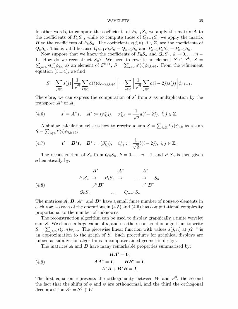
WAVELETS 35
In other words, to compute the coefficients of Pk−1Sn we apply the matrix A tothe coefficients of PkSn, while to compute those of Qk−1Sn we apply the matrixB to the coefficients of PkSn. The coefficients c(j, k), j ∈ Z, are the coefficients ofQkSn. This is valid because Qk−1PkSn = Qk−1Sn and Pk−1PkSn = Pk−1Sn.
Now suppose that we know the coefficients of P0Sn and QkSn, k = 0, . . . , n −1. How do we reconstruct Sn? We need to rewrite an element S ∈ Sk, S =∑j∈Z
s(j)φj,k as an element of Sk+1, S =∑i∈Z
s′(i)φi,k+1. From the refinement
equation (3.1.4), we find
S =∑
j∈Z
s(j)
[1√2
∑
ℓ∈Z
a(ℓ)φℓ+2j,k+1
]=
∑
i∈Z
[1√2
∑
j∈Z
a(i− 2j)s(j)
]φi,k+1.
Therefore, we can express the computation of s′ from s as multiplication by thetranspose A∗ of A:
(4.6) s′ = A∗s, A∗ := (α∗i,j), α∗
i,j :=1√2a(i− 2j), i, j ∈ Z.
A similar calculation tells us how to rewrite a sum S =∑
i∈Zt(i)ψi,k as a sum
S =∑
i∈Zt′(i)φi,k+1:
(4.7) t′ = B∗t, B∗ := (β∗i,j), β∗
i,j :=1√2b(i− 2j), i, j ∈ Z.
The reconstruction of Sn from QkSn, k = 0, . . . , n − 1, and P0Sn is then givenschematically by:
A∗ A∗ A∗
P0Sn → P1Sn → . . . → Sn
ր B∗ ր B∗(4.8)
Q0Sn . . . Qn−1Sn
The matrices A, B, A∗, and B∗ have a small finite number of nonzero elements ineach row, so each of the operations in (4.5) and (4.6) has computational complexityproportional to the number of unknowns.
The reconstruction algorithm can be used to display graphically a finite waveletsum S. We choose a large value of n, and use the reconstruction algorithm to writeS =
∑j∈Z
s(j, n)φj,n. The piecewise linear function with values s(j, n) at j2−n isan approximation to the graph of S. Such procedures for graphical displays areknown as subdivision algorithms in computer aided geometric design.
The matrices A and B have many remarkable properties summarized by:
(4.9)
BA∗ = 0,
AA∗ = I, BB∗ = I,
A∗A+B∗B = I.
The first equation represents the orthogonality between W and S0, the secondthe fact that the shifts of φ and ψ are orthonormal, and the third the orthogonaldecomposition S1 = S0 ⊕W .
36 RONALD A. DEVORE AND BRADLEY J. LUCIER
5. Smoothness Spaces and Wavelet Coefficients
We have seen in §2 that one can determine when a function f ∈ Lp(R) is ina Lipschitz space Lip(α, Lp(R)), 0 < α < 1/p, by examining the coefficients ofthe Haar expansion of f . In fact, one can often characterize membership in generalsmoothness spaces in terms of the size of coefficients in general wavelet or prewaveletexpansions. We do not have the space to explain in detail how such characteriza-tions are proved, but we shall outline one approach, based on approximation, thatparallels the arguments in §2 about Haar wavelets. A more complete presentation,much along the lines given here, can be found in the book of Meyer [Me]. The arti-cle of Frazier and Jawerth [FJ] gives a much more general and extensive treatmentof wavelet-like decompositions from the viewpoint of Littlewood-Paley theory.
We shall suppose that φ satisfies the conditions (3.1.2) of multiresolution. Wealso suppose that φ has compact support. This is not a necessary assumptionfor the characterizations given below (it can be replaced by suitable polynomialdecay at infinity) but it will simplify our discussion. We shall also assume that1 < p < ∞. The arguments that follow can be modified simply to apply whenp = ∞; the analysis for p ≤ 1 can also be developed as below, but then it must becarried out in the setting of the Hardy spaces Hp(R
d).We fix a value of p and let S := S(φ, Lp(Rd)) be the Lp(R
d) closure of the finitelinear combination of shifts of φ.
We assume that the shifts of φ form an Lp(Rd)-stable basis for S. For functions
with compact support, this holds whenever the shifts of φ form an L2(Rd)-stable
basis for S(φ, L2(Rd)) (see Jia and Micchelli [JM]). It follows that the dilated func-
tions φj,k,p := 2k/pφ(2k· − j), j ∈ Zd, form an Lp(Rd)-stable basis of Sk, for each
k ∈ Z. That is, there are constants C1, C2 > 0 such that each S ∈ Sk can berepresented as S =
∑j∈Zd c(j, k, p)(S)φj,k,p with
(5.1) C1
( ∑
j∈Zd
|c(j, k, p)|p)1/p
≤ ‖S‖Lp(Rd) ≤ C2
( ∑
j∈Zd
|c(j, k, p)|p)1/p
.
Next, we show that the orthogonal projector P from L2(Rd) onto S(φ, L2(R
d))has a natural extension to a bounded operator from Lp(R
d) onto S. We can repre-sent P as in (3.2.9):
(5.2) Pf =∑
j∈Z
γj(f)φ( · − j), γj(f) :=
∫
Rd
f(x)γ(x− j) dx.
The function γ ∈ L∞(Rd) decays exponentially at infinity and hence is in Lq(Rd)
for 1 ≤ q ≤ ∞. In particular, γ ∈ Lp′(Rd), and (5.2) serves to define P on Lp(R
d).The compact support of φ and the exponential decay of γ then combine to showthat P is bounded on Lp(R
d). By dilation, we find that the projectors Pk (whichmap Lp(R
d) onto Sk) are bounded independently of k.The projector Q from L2(R
d) onto the wavelet space W is also represented inthe form (5.2) and has an extension to a bounded operator on Lp(R
d) for thesame reasons as above. We can also derive the boundedness of Q from the formulaQ = P1 − P0.
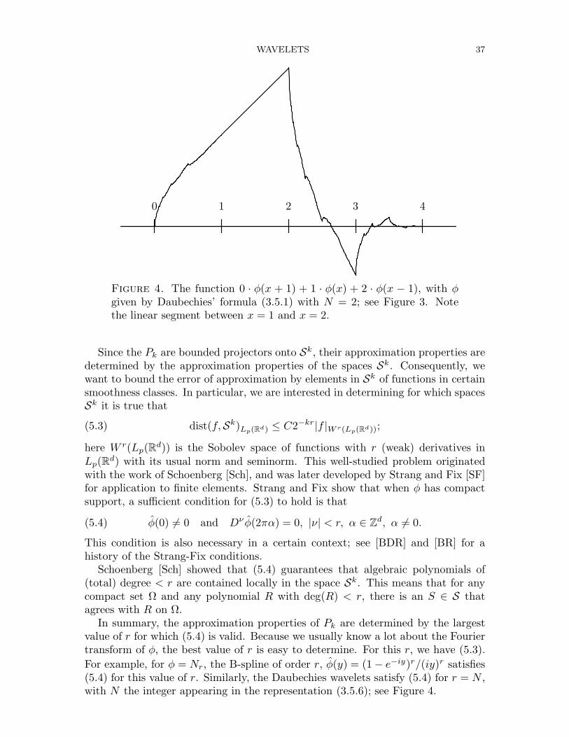
WAVELETS 37
0 1 2 3 4
Figure 4. The function 0 · φ(x + 1) + 1 · φ(x) + 2 · φ(x − 1), with φgiven by Daubechies’ formula (3.5.1) with N = 2; see Figure 3. Notethe linear segment between x = 1 and x = 2.
Since the Pk are bounded projectors onto Sk, their approximation properties aredetermined by the approximation properties of the spaces Sk. Consequently, wewant to bound the error of approximation by elements in Sk of functions in certainsmoothness classes. In particular, we are interested in determining for which spacesSk it is true that
(5.3) dist(f,Sk)Lp(Rd) ≤ C2−kr|f |W r(Lp(Rd));
here W r(Lp(Rd)) is the Sobolev space of functions with r (weak) derivatives in
Lp(Rd) with its usual norm and seminorm. This well-studied problem originated
with the work of Schoenberg [Sch], and was later developed by Strang and Fix [SF]for application to finite elements. Strang and Fix show that when φ has compactsupport, a sufficient condition for (5.3) to hold is that
(5.4) φ(0) 6= 0 and Dν φ(2πα) = 0, |ν| < r, α ∈ Zd, α 6= 0.
This condition is also necessary in a certain context; see [BDR] and [BR] for ahistory of the Strang-Fix conditions.
Schoenberg [Sch] showed that (5.4) guarantees that algebraic polynomials of(total) degree < r are contained locally in the space Sk. This means that for anycompact set Ω and any polynomial R with deg(R) < r, there is an S ∈ S thatagrees with R on Ω.
In summary, the approximation properties of Pk are determined by the largestvalue of r for which (5.4) is valid. Because we usually know a lot about the Fouriertransform of φ, the best value of r is easy to determine. For this r, we have (5.3).
For example, for φ = Nr, the B-spline of order r, φ(y) = (1− e−iy)r/(iy)r satisfies(5.4) for this value of r. Similarly, the Daubechies wavelets satisfy (5.4) for r = N ,with N the integer appearing in the representation (3.5.6); see Figure 4.
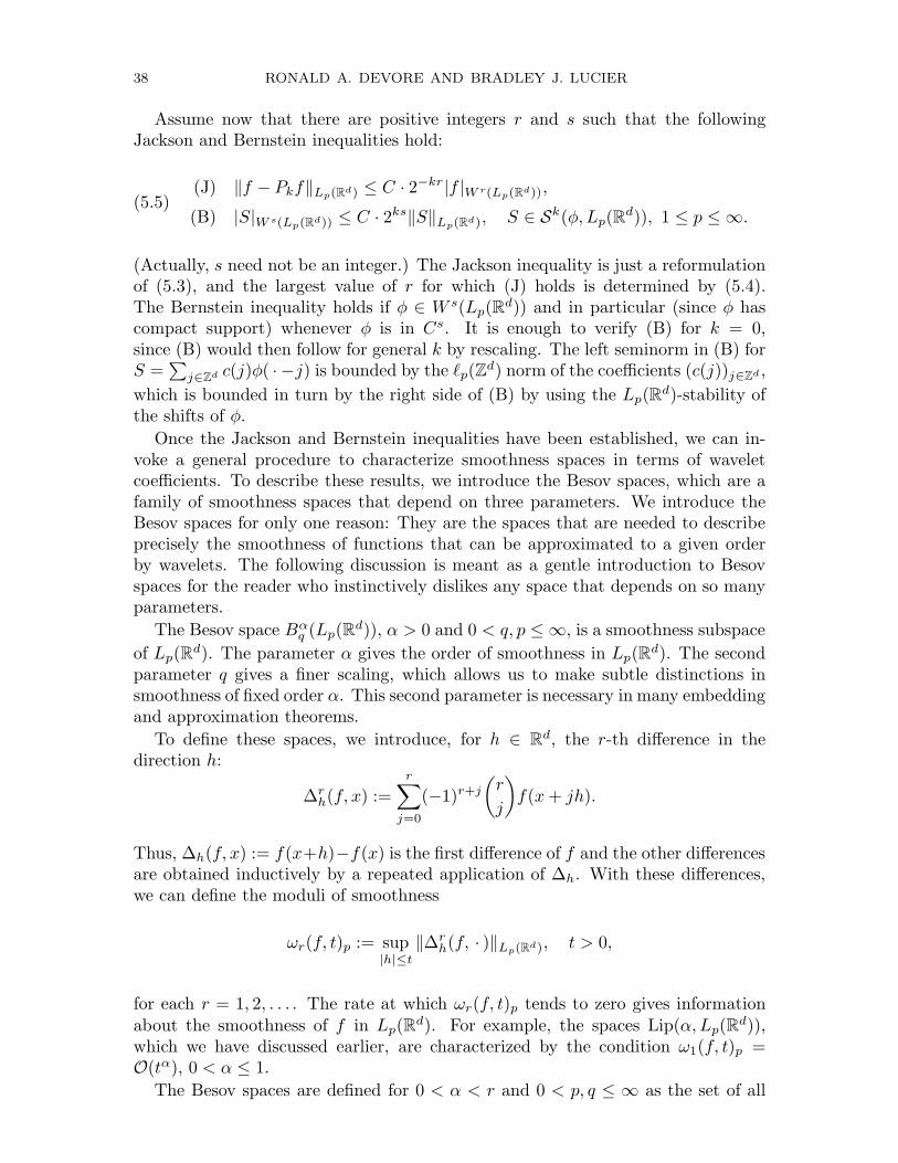
38 RONALD A. DEVORE AND BRADLEY J. LUCIER
Assume now that there are positive integers r and s such that the followingJackson and Bernstein inequalities hold:
(5.5)(J) ‖f − Pkf‖Lp(Rd) ≤ C · 2−kr|f |W r(Lp(Rd)),
(B) |S|W s(Lp(Rd)) ≤ C · 2ks‖S‖Lp(Rd), S ∈ Sk(φ, Lp(Rd)), 1 ≤ p ≤ ∞.
(Actually, s need not be an integer.) The Jackson inequality is just a reformulationof (5.3), and the largest value of r for which (J) holds is determined by (5.4).The Bernstein inequality holds if φ ∈ W s(Lp(R
d)) and in particular (since φ hascompact support) whenever φ is in Cs. It is enough to verify (B) for k = 0,since (B) would then follow for general k by rescaling. The left seminorm in (B) forS =
∑j∈Zd c(j)φ( · −j) is bounded by the ℓp(Z
d) norm of the coefficients (c(j))j∈Zd ,
which is bounded in turn by the right side of (B) by using the Lp(Rd)-stability of
the shifts of φ.
Once the Jackson and Bernstein inequalities have been established, we can in-voke a general procedure to characterize smoothness spaces in terms of waveletcoefficients. To describe these results, we introduce the Besov spaces, which are afamily of smoothness spaces that depend on three parameters. We introduce theBesov spaces for only one reason: They are the spaces that are needed to describeprecisely the smoothness of functions that can be approximated to a given orderby wavelets. The following discussion is meant as a gentle introduction to Besovspaces for the reader who instinctively dislikes any space that depends on so manyparameters.
The Besov space Bαq (Lp(Rd)), α > 0 and 0 < q, p ≤ ∞, is a smoothness subspace
of Lp(Rd). The parameter α gives the order of smoothness in Lp(R
d). The secondparameter q gives a finer scaling, which allows us to make subtle distinctions insmoothness of fixed order α. This second parameter is necessary in many embeddingand approximation theorems.
To define these spaces, we introduce, for h ∈ Rd, the r-th difference in thedirection h:
∆rh(f, x) :=
r∑
j=0
(−1)r+j(r
j
)f(x+ jh).
Thus, ∆h(f, x) := f(x+h)−f(x) is the first difference of f and the other differencesare obtained inductively by a repeated application of ∆h. With these differences,we can define the moduli of smoothness
ωr(f, t)p := sup|h|≤t
‖∆rh(f, · )‖Lp(Rd), t > 0,
for each r = 1, 2, . . . . The rate at which ωr(f, t)p tends to zero gives informationabout the smoothness of f in Lp(R
d). For example, the spaces Lip(α, Lp(Rd)),
which we have discussed earlier, are characterized by the condition ω1(f, t)p =O(tα), 0 < α ≤ 1.
The Besov spaces are defined for 0 < α < r and 0 < p, q ≤ ∞ as the set of all
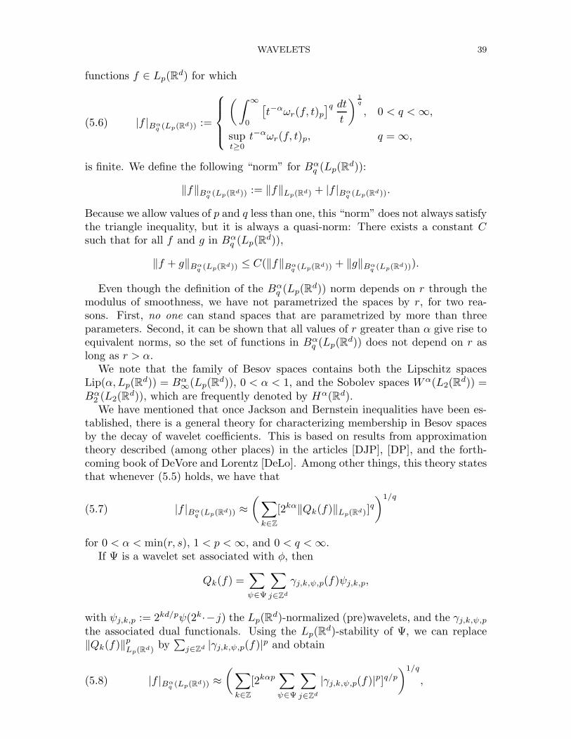
WAVELETS 39
functions f ∈ Lp(Rd) for which
(5.6) |f |Bαq (Lp(Rd)) :=
(∫ ∞
0
[t−αωr(f, t)p
]q dtt
) 1q
, 0 < q <∞,
supt≥0
t−αωr(f, t)p, q = ∞,
is finite. We define the following “norm” for Bαq (Lp(Rd)):
‖f‖Bαq (Lp(Rd)) := ‖f‖Lp(Rd) + |f |Bα
q (Lp(Rd)).
Because we allow values of p and q less than one, this “norm” does not always satisfythe triangle inequality, but it is always a quasi-norm: There exists a constant Csuch that for all f and g in Bαq (Lp(R
d)),
‖f + g‖Bαq (Lp(Rd)) ≤ C(‖f‖Bα
q (Lp(Rd)) + ‖g‖Bαq (Lp(Rd))).
Even though the definition of the Bαq (Lp(Rd)) norm depends on r through the
modulus of smoothness, we have not parametrized the spaces by r, for two rea-sons. First, no one can stand spaces that are parametrized by more than threeparameters. Second, it can be shown that all values of r greater than α give rise toequivalent norms, so the set of functions in Bαq (Lp(R
d)) does not depend on r aslong as r > α.
We note that the family of Besov spaces contains both the Lipschitz spacesLip(α, Lp(R
d)) = Bα∞(Lp(Rd)), 0 < α < 1, and the Sobolev spaces Wα(L2(R
d)) =Bα2 (L2(R
d)), which are frequently denoted by Hα(Rd).We have mentioned that once Jackson and Bernstein inequalities have been es-
tablished, there is a general theory for characterizing membership in Besov spacesby the decay of wavelet coefficients. This is based on results from approximationtheory described (among other places) in the articles [DJP], [DP], and the forth-coming book of DeVore and Lorentz [DeLo]. Among other things, this theory statesthat whenever (5.5) holds, we have that
(5.7) |f |Bαq (Lp(Rd)) ≈
(∑
k∈Z
[2kα‖Qk(f)‖Lp(Rd)]q
)1/q
for 0 < α < min(r, s), 1 < p <∞, and 0 < q <∞.If Ψ is a wavelet set associated with φ, then
Qk(f) =∑
ψ∈Ψ
∑
j∈Zd
γj,k,ψ,p(f)ψj,k,p,
with ψj,k,p := 2kd/pψ(2k·−j) the Lp(Rd)-normalized (pre)wavelets, and the γj,k,ψ,pthe associated dual functionals. Using the Lp(R
d)-stability of Ψ, we can replace‖Qk(f)‖pLp(Rd)
by∑j∈Zd |γj,k,ψ,p(f)|p and obtain
(5.8) |f |Bαq (Lp(Rd)) ≈
(∑
k∈Z
[2kαp∑
ψ∈Ψ
∑
j∈Zd
|γj,k,ψ,p(f)|p]q/p)1/q
,
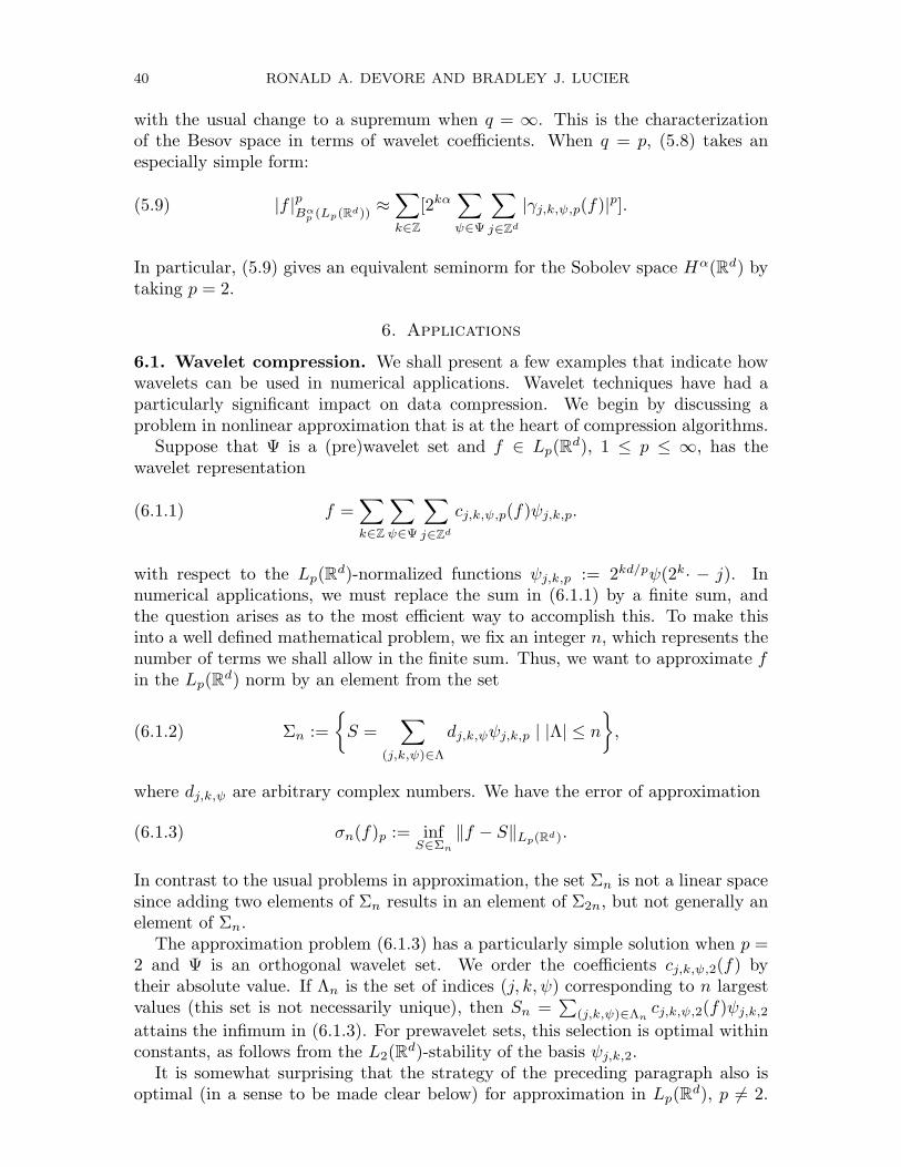
40 RONALD A. DEVORE AND BRADLEY J. LUCIER
with the usual change to a supremum when q = ∞. This is the characterizationof the Besov space in terms of wavelet coefficients. When q = p, (5.8) takes anespecially simple form:
(5.9) |f |pBα
p (Lp(Rd))≈
∑
k∈Z
[2kα∑
ψ∈Ψ
∑
j∈Zd
|γj,k,ψ,p(f)|p].
In particular, (5.9) gives an equivalent seminorm for the Sobolev space Hα(Rd) bytaking p = 2.
6. Applications
6.1. Wavelet compression. We shall present a few examples that indicate howwavelets can be used in numerical applications. Wavelet techniques have had aparticularly significant impact on data compression. We begin by discussing aproblem in nonlinear approximation that is at the heart of compression algorithms.
Suppose that Ψ is a (pre)wavelet set and f ∈ Lp(Rd), 1 ≤ p ≤ ∞, has the
wavelet representation
(6.1.1) f =∑
k∈Z
∑
ψ∈Ψ
∑
j∈Zd
cj,k,ψ,p(f)ψj,k,p.
with respect to the Lp(Rd)-normalized functions ψj,k,p := 2kd/pψ(2k· − j). In
numerical applications, we must replace the sum in (6.1.1) by a finite sum, andthe question arises as to the most efficient way to accomplish this. To make thisinto a well defined mathematical problem, we fix an integer n, which represents thenumber of terms we shall allow in the finite sum. Thus, we want to approximate fin the Lp(R
d) norm by an element from the set
(6.1.2) Σn :=
S =
∑
(j,k,ψ)∈Λ
dj,k,ψψj,k,p | |Λ| ≤ n
,
where dj,k,ψ are arbitrary complex numbers. We have the error of approximation
(6.1.3) σn(f)p := infS∈Σn
‖f − S‖Lp(Rd).
In contrast to the usual problems in approximation, the set Σn is not a linear spacesince adding two elements of Σn results in an element of Σ2n, but not generally anelement of Σn.
The approximation problem (6.1.3) has a particularly simple solution when p =2 and Ψ is an orthogonal wavelet set. We order the coefficients cj,k,ψ,2(f) bytheir absolute value. If Λn is the set of indices (j, k, ψ) corresponding to n largestvalues (this set is not necessarily unique), then Sn =
∑(j,k,ψ)∈Λn
cj,k,ψ,2(f)ψj,k,2attains the infimum in (6.1.3). For prewavelet sets, this selection is optimal withinconstants, as follows from the L2(R
d)-stability of the basis ψj,k,2.It is somewhat surprising that the strategy of the preceding paragraph also is
optimal (in a sense to be made clear below) for approximation in Lp(Rd), p 6= 2.
WAVELETS 41
To describe this, we fix a value of 1 < p < ∞ (slightly weaker results than thosestated below are known when p = ∞) and for f ∈ Lp(R
d), we let Λn denote aset of indices corresponding to n largest values of |cj,k,ψ,p(f)|. We define Sn :=∑
(j,k,ψ)∈Λncj,k,ψ,p(f)ψj,k,p and σn(f)p := ‖f − Sn‖Lp(Rd). DeVore, Jawerth, and
Popov [DJP] have established various results that relate σn(f)p with σn(f)p undercertain conditions on ψ and the generating function φ. For example, it follows fromtheir results that
(6.1.4) σn(f)p = O(n−α/d) ⇐⇒ σn(f)p = O(n−α/d)
for 0 < α < r. Here, the integer r is related to properties of φ. Namely, thegenerating function φ should satisfy the Strang-Fix conditions (5.4) of this orderand φ and ψ should have sufficient smoothness (for example, Cr is enough). It is alsonecessary to assume decay for the functions φ and ψ; sufficiently fast polynomialdecay is enough. We caution the reader that the results in [DJP] are formulatedfor one wavelet ψ and not a wavelet set Ψ. However, the same proofs apply in themore general setting.
It is also of interest to characterize the functions f that satisfy (6.1.4). That is, wewould like to know when we can expect the order of approximation (6.1.4). This hasnot been accomplished in exactly the form of (6.1.4), but the following variant hasbeen shown in [DJP]. The following are equivalent for τ := τ(α, p) := (α/d+1/p)−1:
(6.1.5)
(i)
∞∑
n=1
[nα/dσn(f)p]τ 1
n<∞,
(ii)
∞∑
n=1
[nα/dσn(f)p]τ 1
n<∞,
(iii) f ∈ Bατ (Lτ (Rd)).
Several words of explanation regarding (6.1.5) are in order. First, (6.1.5)(i) isvery close to the condition in (6.1.4). For example, (6.1.5)(i) implies (6.1.4), andif (6.1.4) holds for some β > α then (6.1.5)(i) is valid. So, roughly speaking, itis the functions f ∈ Bατ (Lτ (R
d)) for which the order of approximation in (6.1.4)holds. Secondly, the characterization (6.1.5) says that it is those functions withsmoothness of order α in Lτ (R
d), τ = (α/d+ 1/p)−1, that are approximated withorder O(n−α/d) in Lp(R
d). This should be contrasted with the usual results forapproximation from linear spaces (such as finite element methods), which charac-terize functions with this approximation order as having smoothness of order α inLp(R
d). Since τ < p, the nonlinear approximation problem (6.1.3) provides theapproximation order (6.1.4) for functions with less smoothness than required bylinear methods.
The fact that functions with less smoothness can be approximated well by (6.1.3)is at the essence of wavelet compression. This means that functions with singulari-ties can be handled numerically. Intuitively this is accomplished by retaining in thesum for Sn terms corresponding to functions ψj,k,p that make a large contributionto f near the singularity. Here the situation is similar to adaptive methods for
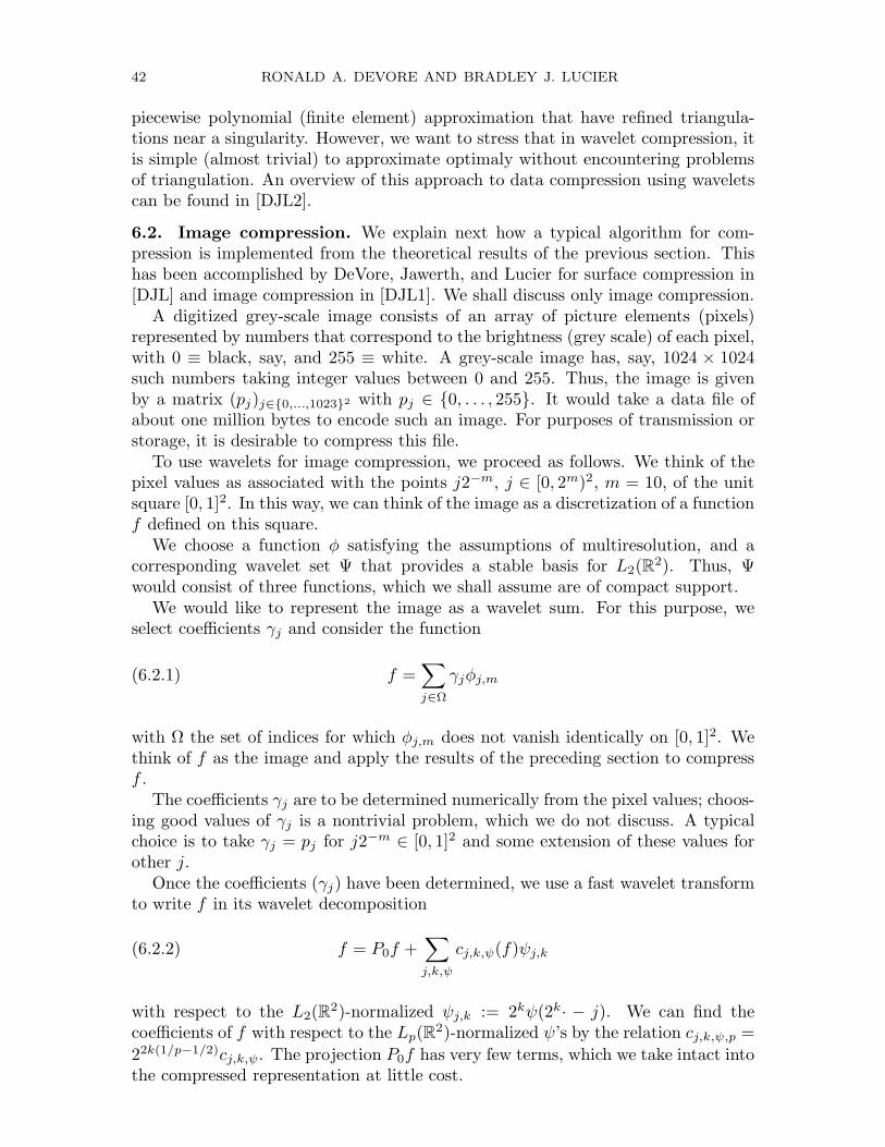
42 RONALD A. DEVORE AND BRADLEY J. LUCIER
piecewise polynomial (finite element) approximation that have refined triangula-tions near a singularity. However, we want to stress that in wavelet compression, itis simple (almost trivial) to approximate optimaly without encountering problemsof triangulation. An overview of this approach to data compression using waveletscan be found in [DJL2].
6.2. Image compression. We explain next how a typical algorithm for com-pression is implemented from the theoretical results of the previous section. Thishas been accomplished by DeVore, Jawerth, and Lucier for surface compression in[DJL] and image compression in [DJL1]. We shall discuss only image compression.
A digitized grey-scale image consists of an array of picture elements (pixels)represented by numbers that correspond to the brightness (grey scale) of each pixel,with 0 ≡ black, say, and 255 ≡ white. A grey-scale image has, say, 1024 × 1024such numbers taking integer values between 0 and 255. Thus, the image is givenby a matrix (pj)j∈0,...,10232 with pj ∈ 0, . . . , 255. It would take a data file ofabout one million bytes to encode such an image. For purposes of transmission orstorage, it is desirable to compress this file.
To use wavelets for image compression, we proceed as follows. We think of thepixel values as associated with the points j2−m, j ∈ [0, 2m)2, m = 10, of the unitsquare [0, 1]2. In this way, we can think of the image as a discretization of a functionf defined on this square.
We choose a function φ satisfying the assumptions of multiresolution, and acorresponding wavelet set Ψ that provides a stable basis for L2(R
2). Thus, Ψwould consist of three functions, which we shall assume are of compact support.
We would like to represent the image as a wavelet sum. For this purpose, weselect coefficients γj and consider the function
(6.2.1) f =∑
j∈Ω
γjφj,m
with Ω the set of indices for which φj,m does not vanish identically on [0, 1]2. Wethink of f as the image and apply the results of the preceding section to compressf .
The coefficients γj are to be determined numerically from the pixel values; choos-ing good values of γj is a nontrivial problem, which we do not discuss. A typicalchoice is to take γj = pj for j2−m ∈ [0, 1]2 and some extension of these values forother j.
Once the coefficients (γj) have been determined, we use a fast wavelet transformto write f in its wavelet decomposition
(6.2.2) f = P0f +∑
j,k,ψ
cj,k,ψ(f)ψj,k
with respect to the L2(R2)-normalized ψj,k := 2kψ(2k· − j). We can find the
coefficients of f with respect to the Lp(R2)-normalized ψ’s by the relation cj,k,ψ,p =
22k(1/p−1/2)cj,k,ψ. The projection P0f has very few terms, which we take intact intothe compressed representation at little cost.
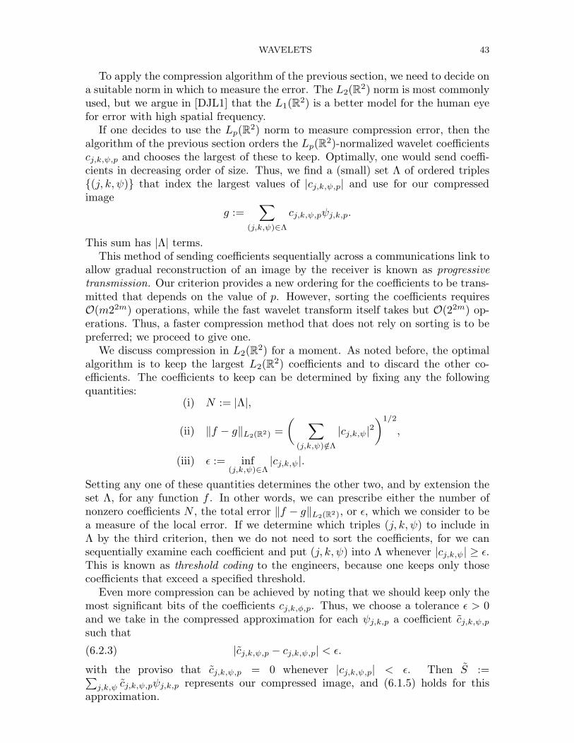
WAVELETS 43
To apply the compression algorithm of the previous section, we need to decide ona suitable norm in which to measure the error. The L2(R
2) norm is most commonlyused, but we argue in [DJL1] that the L1(R
2) is a better model for the human eyefor error with high spatial frequency.
If one decides to use the Lp(R2) norm to measure compression error, then the
algorithm of the previous section orders the Lp(R2)-normalized wavelet coefficients
cj,k,ψ,p and chooses the largest of these to keep. Optimally, one would send coeffi-cients in decreasing order of size. Thus, we find a (small) set Λ of ordered triples(j, k, ψ) that index the largest values of |cj,k,ψ,p| and use for our compressedimage
g :=∑
(j,k,ψ)∈Λ
cj,k,ψ,pψj,k,p.
This sum has |Λ| terms.This method of sending coefficients sequentially across a communications link to
allow gradual reconstruction of an image by the receiver is known as progressive
transmission. Our criterion provides a new ordering for the coefficients to be trans-mitted that depends on the value of p. However, sorting the coefficients requiresO(m22m) operations, while the fast wavelet transform itself takes but O(22m) op-erations. Thus, a faster compression method that does not rely on sorting is to bepreferred; we proceed to give one.
We discuss compression in L2(R2) for a moment. As noted before, the optimal
algorithm is to keep the largest L2(R2) coefficients and to discard the other co-
efficients. The coefficients to keep can be determined by fixing any the followingquantities:
(i) N := |Λ|,
(ii) ‖f − g‖L2(R2) =
( ∑
(j,k,ψ)/∈Λ
|cj,k,ψ|2)1/2
,
(iii) ǫ := inf(j,k,ψ)∈Λ
|cj,k,ψ|.
Setting any one of these quantities determines the other two, and by extension theset Λ, for any function f . In other words, we can prescribe either the number ofnonzero coefficients N , the total error ‖f − g‖L2(R2), or ǫ, which we consider to bea measure of the local error. If we determine which triples (j, k, ψ) to include inΛ by the third criterion, then we do not need to sort the coefficients, for we cansequentially examine each coefficient and put (j, k, ψ) into Λ whenever |cj,k,ψ| ≥ ǫ.This is known as threshold coding to the engineers, because one keeps only thosecoefficients that exceed a specified threshold.
Even more compression can be achieved by noting that we should keep only themost significant bits of the coefficients cj,k,φ,p. Thus, we choose a tolerance ǫ > 0and we take in the compressed approximation for each ψj,k,p a coefficient cj,k,ψ,psuch that
(6.2.3) |cj,k,ψ,p − cj,k,ψ,p| < ǫ.
with the proviso that cj,k,ψ,p = 0 whenever |cj,k,ψ,p| < ǫ. Then S :=∑j,k,ψ cj,k,ψ,pψj,k,p represents our compressed image, and (6.1.5) holds for this
approximation.
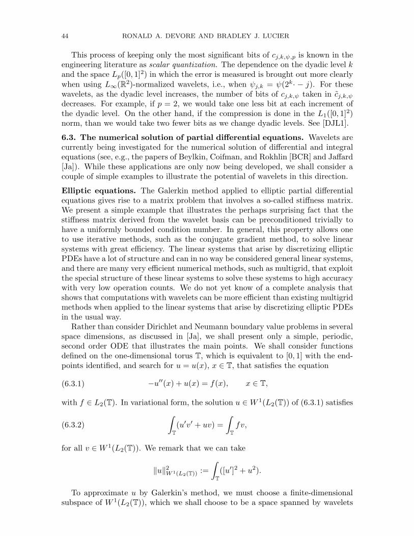
44 RONALD A. DEVORE AND BRADLEY J. LUCIER
This process of keeping only the most significant bits of cj,k,ψ,p is known in theengineering literature as scalar quantization. The dependence on the dyadic level kand the space Lp([0, 1]
2) in which the error is measured is brought out more clearlywhen using L∞(R2)-normalized wavelets, i.e., when ψj,k = ψ(2k· − j). For thesewavelets, as the dyadic level increases, the number of bits of cj,k,ψ taken in cj,k,ψdecreases. For example, if p = 2, we would take one less bit at each increment ofthe dyadic level. On the other hand, if the compression is done in the L1([0, 1]
2)norm, than we would take two fewer bits as we change dyadic levels. See [DJL1].
6.3. The numerical solution of partial differential equations. Wavelets arecurrently being investigated for the numerical solution of differential and integralequations (see, e.g., the papers of Beylkin, Coifman, and Rokhlin [BCR] and Jaffard[Ja]). While these applications are only now being developed, we shall consider acouple of simple examples to illustrate the potential of wavelets in this direction.
Elliptic equations. The Galerkin method applied to elliptic partial differentialequations gives rise to a matrix problem that involves a so-called stiffness matrix.We present a simple example that illustrates the perhaps surprising fact that thestiffness matrix derived from the wavelet basis can be preconditioned trivially tohave a uniformly bounded condition number. In general, this property allows oneto use iterative methods, such as the conjugate gradient method, to solve linearsystems with great efficiency. The linear systems that arise by discretizing ellipticPDEs have a lot of structure and can in no way be considered general linear systems,and there are many very efficient numerical methods, such as multigrid, that exploitthe special structure of these linear systems to solve these systems to high accuracywith very low operation counts. We do not yet know of a complete analysis thatshows that computations with wavelets can be more efficient than existing multigridmethods when applied to the linear systems that arise by discretizing elliptic PDEsin the usual way.
Rather than consider Dirichlet and Neumann boundary value problems in severalspace dimensions, as discussed in [Ja], we shall present only a simple, periodic,second order ODE that illustrates the main points. We shall consider functionsdefined on the one-dimensional torus T, which is equivalent to [0, 1] with the end-points identified, and search for u = u(x), x ∈ T, that satisfies the equation
(6.3.1) −u′′(x) + u(x) = f(x), x ∈ T,
with f ∈ L2(T). In variational form, the solution u ∈W 1(L2(T)) of (6.3.1) satisfies
(6.3.2)
∫
T
(u′v′ + uv) =
∫
T
fv,
for all v ∈W 1(L2(T)). We remark that we can take
‖u‖2W 1(L2(T)):=
∫
T
([u′]2 + u2).
To approximate u by Galerkin’s method, we must choose a finite-dimensionalsubspace of W 1(L2(T)), which we shall choose to be a space spanned by wavelets
WAVELETS 45
defined on the circle T. We indicate briefly how to construct periodic wavelets onT from wavelets on R.
For any f with compact support defined on R, the function
f :=∑
j∈Z
f(·+ j)
is a function of period one, which we call the periodization of f . To obtain waveletson T, we apply this periodization to wavelets on R. To be specific, we consideronly the Daubechies wavelets ψ := D2N with N > 2 because they are contained inW 1(L2(T)). (The first nontrivial Daubechies wavelet, D4, is in W
α(L2(T)) for allα < 1 (see [E]), but we do not know if it is in W 1(L2(T)).) Let φ be the function of§3.5 that gives rise to ψ. For each k ∈ Z, we let φj,k and ψ
j,k be the periodization
of the functions φj,k and ψj,k respectively. We define Sk to be the linear span of thefunctions φj,k, j = 0, . . . , 2k − 1. The functions in this space are clearly of periodone. We also note that the φj,k are orthogonal. Indeed, because they are periodic,
∫ 1
0
φj,kφj′,k =
∑
ℓ∈Z
∫ 1
0
φj,k( · + ℓ)φj′,k =∑
ℓ∈Z
∫ 1
0
φj,k( · + ℓ)φj′,k( · + ℓ)
=
∫
R
φj,kφj′,k =
∑
ℓ∈Z
∫
R
φj,kφj′,k( · + ℓ) =∑
ℓ∈Z
∫
R
φj,kφj′+ℓ2k,k.
If j 6= j′, each integral in the last sum is zero, since we never have j = j′ + 2kℓ.If j = j′, then exactly one integral in the last sum is nonzero and its value is one.Similarly, we find that ψ
j,k, j = 0, . . . , 2k − 1, k ≥ 0, is an orthonormal system for
L2(T). It is easy to check that by adjoining φ0,0, which is identically one on T, thisorthonormal system is complete.
Returning to our construction of periodic wavelet spaces, we define W k to bethe linear span of the functions ψ
j,k, j = 0, . . . , 2k − 1. Then Sk+1 = Sk ⊕ W k. Tosimplify our notation in this section, in which we refer to periodic wavelets only, wedrop the superscripts and tildes, and denote by φj,k, ψj,k, Sk, andW k, the periodicwavelet bases and spaces.
Returning to the numerical solution of (6.3.1), we choose a positive value of mand approximate u by an element um ∈ Sm that satisfies:
(6.3.3)
∫
T
(u′mv′ + umv) =
∫
T
fv, v ∈ Sm.
We can write um and v as in (6.2.2). For example,
(6.3.4) um = P0um +
m−1∑
k=0
Qkum = γφ0,0 +
m−1∑
k=0
2k−1∑
j=0
β(j, k)ψj,k.
Because φ0,0 is identically one on the circle T, γ is just the average of um on T.From (6.3.3) we see that with v ≡ 1, γ =
∫Tf . Thus, we need to determine β(j, k).
46 RONALD A. DEVORE AND BRADLEY J. LUCIER
If we replace um in (6.3.3) by its representation (6.3.4), we arrive at a system ofequations
m−1∑
k=0
2k−1∑
j=0
β(j, k)
∫
T
(ψ′j,kψ
′j′,k′ + ψj,kψj′,k′) =
∫
T
fψj′,k′ ,
for j′ = 0, . . . , 2k′ − 1 and k′ = 0, . . . , m− 1, or, more succinctly,
(6.3.5) Tβ = f
where the typical entry in T is∫T(ψ′j,kψ
′j′,k′ + ψj,kψj′,k′) and f a vector with
components∫Tfψj′,k′ ; β = (β(j, k))j=0,...,2k−1, k=0,...,m−1 is the coefficient vector
of the unknown function.The convergence rate of the conjugate gradient method, a popular iterative
method for the solution of systems like (6.3.5), depends on the condition number,κ(T ) = ‖T‖‖T−1‖, of the symmetric, positive definite, stiffness matrix T . Now,
‖T‖ = sup‖α‖
ℓ2=1
α∗Tα and ‖T−1‖−1 = inf‖α‖ℓ2=1
α∗Tα,
where α := (α(j, k))j=0,...,2k−1, k=0,...,m−1. For any vector α, we form the functionS := S(α) ∈ Sm by
S =
m−1∑
k=0
2k−1∑
j=0
α(j, k)ψj,k.
For example, um = γφ0,0 + S(β). It follows easily that
(6.3.6) |α∗Tα| =∫ 1
0
([S′]2 + S2) = ‖S‖2W 1(L2(Rd)) ≈m−1∑
k=0
2k−1∑
j=0
|2kα(j, k)|2.
The last equivalence in (6.3.6) is a variant of (5.9) (for q = p = 2). In (5.9), weconsidered wavelet representations beginning at the dyadic level k = −∞; we couldjust as easily have begun at the level k = 0 (by including P0) and arrived at theequivalence in (6.3.6).
Equation (6.3.6) shows that the matrix DTD, where D has entries 2−kδjj′δkk′ ,
satisfies
|α∗DTDα| ≈m−1∑
k=0
2k−1∑
j=0
|α(j, k)|2;
i.e., the stiffness matrix T can be trivially preconditioned to have a condition num-ber κ(DTD) := ‖DTD‖‖D−1T−1D−1‖ that is bounded independently of m.
Because the subspace Sm of L2(T) generated by the Daubechies wavelet D2N
locally contains all polynomials of degree < N , we have that
infv∈Sm
‖u− v‖W 1(L2(T)) ≤ C2−m(N−1)|u|WN (L2(T)).
WAVELETS 47
Because of the special form of (6.3.1), um is in fact the W 1(L2(T)) projection of uonto Sm, so we have
‖u− um‖W 1(L2(T)) ≤ C2−m(N−1)|u|WN (L2(T)).
One can treat in an almost identical way the equation (6.3.1) defined on thetorus Td with the left side replaced by −∇ · (a∇u) + bu with a and b bounded,smooth, positive functions on Td, and obtain the same uniform bound on the con-dition number. Of course, ultimately, one would like to handle elliptic boundaryvalue problems for a domain Ω. First results in this direction have been obtainedby Jaffard [Ja] and in a slightly different (nonwavelet) setting by Oswald (see forexample [O]). For example, Jaffard’s approach to elliptic equations with Dirichletboundary conditions is to transform the equation to one with zero boundary con-ditions by extending the boundary function into the interior of the domain Ω. Hethen employs in a Galerkin method wavelets whose support is contained strictlyinside Ω. However, there has not yet been an analysis of the desired relationshipbetween the extension and the wavelets employed. Another approach is to developwavelets for the given domain (which do not vanish on the boundary) (see [JaMe]).
Employing wavelets for elliptic problems as outlined above is similar to the useof hierarchical bases in the context of multigrid. However, two points suggest thatwavelet bases may be more useful than hierarchical bases. First, the wavelet basesare L2(R
d)-stable, while the hierarchical basis are not. Second, one can choosefrom a much greater variety of wavelet bases with various approximation properties(values of N).
Finally, we mention the great potential for compression to be used in conjunctionwith wavelets for elliptic problems in a similar way to adaptive finite elements (seealso [Ja]).
6.4. Time dependent problems. Wavelets have potential application for the nu-merical solution of time-dependent parabolic and hyperbolic problems. We mentionone particular application where the potential of wavelets has at least theoreticalfoundation.
We consider the solution u(x, t) of the scalar hyperbolic conservation law
(6.4.1)ut + f(u)x = 0, x ∈ R, t > 0,
u(x, 0) = u0(x), x ∈ R,
in one space dimension. It is well known that the solution to (6.4.1) developsdiscontinuities (called “shocks”) even when the initial condition is smooth. Thismakes the numerical treatment of (6.4.1), and even more so its analogue in severalspace dimensions, somewhat subtle. The appearance of shocks calls for adaptive ornonlinear methods.
Considering the appearance of discontinuities in the solution u to (6.4.1), thefollowing regularity result of the authors [DL], [DL1], is quite surprising. If the fluxf in (6.4.1) is strictly convex and suitably smooth, and u0 has bounded variation,then it has been shown that for any α > 0 and τ := τ(α) := (α+ 1)−1,
(6.4.2) u0 ∈ Bατ (Lτ (R)) =⇒ u( · , t) ∈ Bατ (Lτ (R)),
48 RONALD A. DEVORE AND BRADLEY J. LUCIER
for all later time t > 0. That is, if u0 has smoothness of order α in Lτ (R) then sowill u( · , t) for all later time t > 0.
The regularity result (6.4.2) has an interpretation in terms of wavelet decom-positions. We cannot use orthogonal wavelets in these decompositions because,as we pointed out earlier, they do not provide stable representations of functionsin L1(R) because they have mean value zero. However, the characterization ofBesov spaces can be carried out using other, nonorthogonal, wavelets, such as B-splines. With this caveat, (6.4.2) says that whenever u0 has a wavelet decomposition∑j,k∈Z
γj,k(u0)ψj,k,1, with certain L1(R)-normalized wavelets ψ, whose coefficientssatisfy
(6.4.3)∑
k∈Z
∑
j∈Z
|γj,k(u0)|τ <∞,
then u( · , t) has a similar wavelet decomposition with the same control (6.4.3) on thecoefficients. We want to stress that the results in [DL] and [DL1] do not describedirectly how to determine wavelet coefficients at later time t > 0 from those ofthe initial function u0. That is, there is no direct, theoretically correct, numericalmethod known to us that describes how to update coefficients with time so that(6.4.3) holds. The regularity result (6.4.2) is proved by showing that whenever u0can be approximated well in L1(R) by piecewise polynomials with free (variable)knots, then u( · , t) can be approximated in the same norm by piecewise algebraicfunctions (of a certain type) with free knots.
Finally, we mention that the authors have also shown that the analogue of regu-larity result (6.4.3) does not hold in more than one space dimension. From the pointof view of wavelet decompositions, our results seem to indicate that the waveletsdescribed in this presentation are too symmetric to effectively handle the diversetypes of singularities that arise in the solution of conservation laws in several spacedimensions.
References
[Ba] G. Battle, A block spin construction of ondelettes, Part I: Lemarie functions, Comm.Math. Phys. 110 (1987), 601–615.
[B-AR] A. Ben Artzi and A. Ron, On the integer translates of a compactly supported function:
Dual bases and linear projectors, SIAM J. Math. Anal. 21 (1990), 1550–1562.
[BCR] G. Beylkin, R. Coifman, and V. Rokhlin, Fast wavelet transforms and numerical algo-
rithms I, Comm. Pure and Appl. Math. XLIV (1991), 141–183.
[BDR] C. de Boor, R. DeVore and A. Ron, Approximation from shift invariant spaces, preprint.
[BDR1] C. de Boor, R. DeVore and A. Ron, Wavelets and prewavelets, preprint.
[BDR2] C. de Boor, R. DeVore and A. Ron, The structure of finitely generated shift invariant
spaces in L2(Rd), preprint.
[BR] C. de Boor and A. Ron, Fourier analysis of the approximation power of principal shift-
invariant spaces, Constructive Approximation 8 (1992), 427–462.
[CDM] A. Cavaretta, W. Dahmen and C. Micchelli, Subdivision for Computer Aided Geometric
Design, Memoirs Amer. Math. Soc. 93 (1991).
[CSW] C. K. Chui, J. Stockler and J. D. Ward, Compactly supported box-spline wavelets, CATReport, Texas A& M University 230 (1991).
[CW] C. K. Chui and J. Z. Wang, On compactly supported spline wavelets and a duality prin-
ciple, Trans. Amer. Math. Soc. (1991).
WAVELETS 49
[CW1] C. K. Chui and J. Z. Wang, A general framework for compactly supported splines and
wavelets, CAT Report, Texas A&M University 219 (1990).
[DM] W. Dahmen and C. Micchelli, On stationary subdivision and the construction of com-
pactly supported wavelets, Multivariate Approximation and Interpolation (W. Haussmann
and K. Jetter, eds.), ISNM vol. 94, Birkhauser Verlag, 1990, pp. 69–89.
[Da] I. Daubechies, Orthonormal bases of compactly supported wavelets, Comm. on Pure andAppl. Math. XLI (1988), 909–996.
[Da1] I. Daubechies, The wavelet transform, time-frequency localization and signal analysis,
IEEE Trans. on Information Theory 36 (1990), 961–1005.
[DJL] R. DeVore, B. Jawerth, and B. Lucier, Surface compression, Computer Aided GeometricDesign 9 (1992), 219–239.
[DJL1] R. DeVore, B. Jawerth, and B. Lucier, Image compression through wavelet transform
coding, IEEE Transactions on Information Theory 38 (1992), 719–746, Special Issue onWavelet Transforms and Multiresolution Signal Analysis.
[DJL2] R. DeVore, B. Jawerth, and B. Lucier, Data compression using wavelets: Error, smooth-
ness, and quantization, DCC-91, Data Compression Conference (J. A. Storer and J. H.Reif, eds.), IEEE Computer Society Press, Los Alamitos, CA, 1991, pp. 186–195.
[DJP] R. DeVore, B. Jawerth, and V. Popov, Compression of wavelet decompositions, Amer. J.
Math. (to appear).
[DeLo] R. DeVore and G. Lorentz, Constructive Approximation, Springer Grundlehren, Heidel-berg, 1992.
[DL] R. DeVore and B. Lucier, High order regularity for conservation laws, Indiana Univ.
Math. J. 39 (1990), 413–430.
[DL1] R. DeVore and B. Lucier, High order regularity for solutions of the inviscid Burgers equa-
tion, Nonlinear Hyperbolic Problems (Proceedings of an Advanced Research Workshop,
Bordeaux, France, June 1988, Springer Lecture Notes in Mathematics, vol. 1402) (C.
Carasso, P. Charrier, B. Hanouzet, J.-L. Joly, eds.), Springer-Verlag, New York, 1989,pp. 147–154.
[DP] R. DeVore and V. Popov, Interpolation spaces and non-linear approximation, Function
Spaces and Applications (M. Cwikel, J. Peetre, Y. Sagher, and H. Wallin, eds.), SpringerLecture Notes in Mathematics, vol. 1302, Springer, New York, 1988, pp. 191–205.
[E] T. Eirola, Sobolev characterization of solutions of dilation equations, SIAM J. Math.
Anal. (to appear).
[FJ] M. Frazier and B. Jawerth, A discrete transform and decompositions of distribution
spaces, J. of Functional Anal. 93 (1990), 34–170.
[FJW] M. Frazier, B. Jawerth, and G. Weiss, Littlewood-Paley Theory and the Study of Function
Spaces, Conference Board of the Mathematical Sciences, Regional Conference Series in
Mathematics, Number 79, American Mathematical Society, Providence, RI, 1991.
[Ja] S. Jaffard, Wavelet methods for fast resolution of elliptic problems, preprint.
[JaMe] S. Jaffard and Y. Meyer, Bases ondelettes dans des ouverts de Rn, Jour. Math. Pures et
Appl. 68 (1989), 95–108.
[JM] R-Q. Jia and C. Micchelli, Using the refinement equation for the construction of pre-
wavelets II: power of two, Curves and Surfaces (P. J. Laurent, A. LeMehaute, and L.
Schumaker, eds.), Academic Press, New York, 1991, pp. 209–246.
[KS] S. Karlin and W. Studden, Tchebycheff Systems with Application to Analysis and Sta-
tistics, Wiley Interscience, New York, 1966.
[LM] R. A. H. Lorentz and W. R. Madych, Wavelets and generalized box splines, preprint.
[Ma] S. G. Mallat, Multiresolution approximations and wavelet orthonormal bases of L2(R),
Trans. Amer. Math. Soc 315 (1989), 69–87.
[Me] Y. Meyer, Ondelettes et Operateurs I: Ondelettes, Hermann, 1990.
[Me1] Y. Meyer, Wavelets with compact support, Zygmund Lectures (University of Chicago),1987.
[Mi] C. Micchelli, Using the refinement equation for the construction of pre-wavelets, Numer-
ical Algorithms 1 (1991), 75–116.
[0] P. Oswald, On discrete norm estimates related to multilevel preconditioners in the finite
elment method, preprint.
50 RONALD A. DEVORE AND BRADLEY J. LUCIER
[RS] S. D. Riemenschneider and Z. W. Shen, Box splines, cardinal splines, and wavelets,
Approximation Theory and Functional Analysis (C. K. Chui, ed.), Academic Press, NewYork, 1991, pp. 133–149.
[RS1] S. D. Riemenschneider and Z. W. Shen, Wavelets and prewavelets in low dimensions, J.Approx. Theory (to appear).
[RV] O. Rioul and M. Vetterli, Wavelets and signal processing, IEEE Signal Processing Mag-
azine 8 (1991), no. 4, 14–38.[Sch] I. Schoenberg, Contributions to the problem of approximation of equidistant data by
analytic functions, Parts A & B, Quarterly Appl. Math. IV (1946), 45–99, 112–141.
[Sch1] I. Schoenberg, Cardinal Spline Interpolation, Regional Conference Series in AppliedMathematics, vol. 12, SIAM, Philadelphia, 1973.
[SF] G. Strang and G. Fix, A Fourier analysis of the finite element variational method,C.I.M.E. II Ciclo 1971, Constructive Aspects of Functional Analysis (G. Geymonat, ed.),
1973, pp. 793–840.
[St] J. O. Stromberg, A modified Franklin system and higher-order spline systems on Rn
as unconditional basis for Hardy spaces, Conference in Harmonic Analysis in Honor of
Antoni Zygmund (W. Beckner et al., ed., eds.), vol. Vol II, Wadsworth, 1981, pp. 475–493.
Department of Mathematics, University of South Carolina, Columbia, SC 29208
Department of Mathematics, Purdue University, West Lafayette, IN 47907