Waves Incident on a Circular Harbour

Waves Incident on a Circular HarbourAuthor(s): A. BurrowsSource: Proceedings of the Royal Society of London. Series A, Mathematical and PhysicalSciences, Vol. 401, No. 1821 (Oct. 8, 1985), pp. 349-371Published by: The Royal SocietyStable URL: http://www.jstor.org/stable/2397894 .

Accessed: 12/06/2014 20:46

Your use of the JSTOR archive indicates your acceptance of the Terms & Conditions of Use, available at .http://www.jstor.org/page/info/about/policies/terms.jsp

.JSTOR is a not-for-profit service that helps scholars, researchers, and students discover, use, and build upon a wide range ofcontent in a trusted digital archive. We use information technology and tools to increase productivity and facilitate new formsof scholarship. For more information about JSTOR, please contact [email protected].

.

The Royal Society is collaborating with JSTOR to digitize, preserve and extend access to Proceedings of theRoyal Society of London. Series A, Mathematical and Physical Sciences.

http://www.jstor.org

This content downloaded from 185.44.77.82 on Thu, 12 Jun 2014 20:46:51 PMAll use subject to JSTOR Terms and Conditions

http://www.jstor.org/action/showPublisher?publisherCode=rsl

http://www.jstor.org/stable/2397894?origin=JSTOR-pdf

http://www.jstor.org/page/info/about/policies/terms.jsp


Proc. R. Soc. Lond. A 401, 349-371 (1985) 349 Printed in Great Britain

Waves incident on a circular harbour

BY A. BURROWS

Department of Mathematics, Manchester University, Manchester Ml 3 9PL, U.K.

(Communicated by F. Ursell, F.R.S. - Received 1 May 1985)

The wave amplitude inside a harbour that is subject to incident waves is greatly affected by the frequency of the incident waves. If the harbour entrance is small it is expected that the internal resonances of the harbour will be excited at the appropriate incident frequencies. Published arguments concerning the magnitude of the resonances are, however, not conclusive. In this paper a circular harbour with a small entrance is studied with the use of a rigorous mathematical treatment. It is found that as the harbour entrance decreases in size the magnitude of resonance owing to a single frequency increases slowly (logarithmically). However, this increase is too slow to make a significant difference. The magnitude of resonance in relation to a continuous spectrum input increases, but for the Helmholtz mode only. Again the increase is slow (logarithmic). These results are found to be in agreement with the work of J. Miles (J. Fluid Mech. 46, 241-265 (1971)).

In many approximate calculations it is assumed that the total flow through the gap will effectively determine the flow near a resonant frequency. This is correct near the Helmholtz resonance, but incorrect near the higher resonances where the through-flow is small.

INTRODUCTION

When a harbour is subject to incident waves it is found that the wave amplitude inside the harbour is greatly affected by the frequency of the incident waves. At certain frequencies the harbour acts as a resonator and the wave amplitude is comparatively large. When a harbour is closed and the damping is neglected, the free-wave motion is known to be the superposition of normal modes of standing waves with a discrete spectrum of characteristic frequencies. When a harbour has a small opening and is subject to incident waves we may expect a resonance whenever the frequency of the incident waves is close to a characteristic frequency of the closed harbour. A resonance of a different type is given by the so-called Helmholtz mode when the oscillatory motion inside the harbour is much slower than each of the normal modes.

The oscillation of harbours (and the analogous problem for acoustic resonators) has been investigated by many authors. In particular, Miles & TMunk (1961) investigated the response of a harbour to a broad-band input of frequencies centred around one of the internal resonant frequencies (by the 'response' we shall henceforth mean the ultimate periodic steady-state response of the harbour), by treating the harbour as an equivalent mechanical (or acoustic) forced oscillator.

[ 349 ]



350 A. Burrows

They concluded that the mean squared response to a continuous broad-band input (defined as the power transfer factor, P) increases as the gap decreases, for all modes of resonance. This paradoxical result they termed the 'harbour paradox'. (If the gap is very small it will clearly take a long time to attain the ultimate steady state.) in later work, Miles (I97I) treated the problem by an equivalent-circuit analysis (which is no longer familiar) and reached a different conclusion: the harbour paradox holds for the Helmholtz mode but not for the higher modes for which the power transfer varies insignificantly as the width of the gap decreases. In view of these differing conclusions it may be useful to treat a harbour of very simple shape by a more direct and mathematically rigorous method.

We shall consider a circular harbour, consisting of a fixed vertical cylinder with a narrow slit from top to bottom, in an inviscid fluid of constant depth (figure 1).

z h

FIGURE 1. Description of the problem and definition of coordinates. We consider a circular harbour consisting of a fixed vertical cylinder of radius a, with a gap facing incident waves in fluid of constant depth, h. The angle subtended by the gap from the centre is 2ac rad.

We assume incident waves coming from infinity, directly facing the gap, and make no provision for a coastline. We also assume that the motion is irrotational, has periodic time dependence and that small-amplitude wave theory is applicable. It will be shown that the problem is equivalent to a two-dimensional sound-wave problem: a circular arc facing incident sound waves. This two-dimensional problem can be solved as follows. As an unknown function we choose V(O), the radial velocity in the gap, so that the interior and exterior motions can be expressed in terms of V(O). Because the potential across the gap is continuous we obtain an integral equation of the first kind for V(O). We next show that this equation can be transformed into an equation of the second kind, whose solution we can find (when the gap is small) from the Neumann series. In ? 1 we develop the mathematical model and reduce the problem to that of solving an integral equation of the first kind for V(O). In ?2 we find V(O) by the above method. In ??3 and 4 we apply the results to find the surface displacement and measures of amplification in the required modes of resonance. It will be assumed that the wavelength exceeds the width of the gap.

1. REDUCTION TO AN INTEGRAL EQUATION

We consider a circular harbour as shown in figure 1, which consists of a fixed vertical cylinder, with a gap facing incident waves coming from infinity. We let the fluid be of constant depth, h, the radius of the harbour be a, and the angle



Waves incident on a circular harbour 351

subtended by the gap from the centre be 2a, as shown. We take Cartesian and cylindrical polar coordinates as shown, with the origin at the centre of the harbour. We assume that the motion is irrotational and that the fluid is inviscid, so that we can define a velocity potential P. We further assume that the motion is periodic with respect to time, so that

O(x,y,z,t) = P(x,y,z)e-iwt

We specify the following boundary conditions:

aOlaz = 0 on z = h, for no flow through the floor;

aOlar Ir=a = 0 for I 0 1 > a, for no flow across the harbour wall;

and by assuming that small-amplitude wave theory is applicable, we also specify

KP + aP/az = 0 on z = 0, the free surface condition given periodic time dependence

(see, for example, Stoker (I 957), chapter 2, ?1), where K = 02/g.

From the equation of continuity we know that

V2' = O.

If we consider (x, y) fixed, then because P is continuous as a function of z, and also d'/dz exists and is continuous as a function of z, we can expand ( in the form

cosh k(h -z) "Ocoskm (h -z) (x, y, Z) =

cosh (kh)

c(X,

y) + E cos (k h)

5 m(X, Y),

where cos km (h - z) are the eigenfunctions of

[d2/dz2 + km] 6 = 0

such that (K+d/dz)6 = 0 on z = O,

and d6/dz = 0 on z = h

(so that w02/g = k-m tan (km h)); and where cosh k(h - z) is the eigenfunction of

(d2/dz2 -k2)6 = 0

such that (K+d/dz)6=0 on z=O,

and d6/dz = 0 on z = h

(so that k tanh (kh) = (02/g). The above expansion for P is the Sturm-Liouville expansion (see, for example,

Titchmarsh (1946), theorem (1.9)), and holds for all x, y. The functions O5m and 54 must satisfy the equations

(V2-k24m = 0

and (V2+k2) 4 = 0;



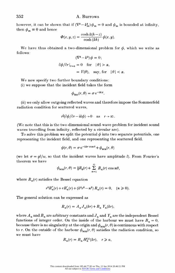
352 A. Burrows

however, it can be shown that if (V2 - k 2) Vm = 0 and 5Im is bounded at infinity, then O6m =0 and hence

O(X Y Z =cosh k(h -z) 0(,Y 'P(a,y,z) = cosh (kh) 5(x'y)

We have thus obtained a two-dimensional problem for 54, which we write as follows:

(V2 - k2) S = 0;

d4/dr Ir=a = 0 for I 0 | > a,

=V(O), say,for IOI< a.

We now specify two further boundary conditions: (i) we suppose that the incident field takes the form

= .ikx. sSinc (r, ) = a- e-iX

(ii) we only allow outgoing reflected waves and therefore impose the Sommerfeld radiation condition for scattered waves,

r1(0SO/dr-ikO)-?0. as r- -oo.

(We note that this is the two-dimensional sound-wave problem for incident sound waves travelling from infinity, reflected by a circular arc).

To solve this problem we split the potential 5S into two separate potentials, one representing the incident field, and one representing the scattered field.

I(r ) = .e-ikrcosO+q5sca(r, )

(we let o. = gliw, so that the incident waves have amplitude 1). From Fourier's theorem we have

V6sca(r, 0) = -Ro(r)+ Rn (r) cos nO, n=1

where Rn(r) satisfies the Bessel equation

r2R' (r)+rB (r)+(k2r2-n2)Rn(r) = 0, (n > 0).

The general solution can be expressed as

Rn(r) = An Jn(kr) + Bn Yn(kr),

where An and Bn are arbitrary constants and Jn and Yn are the independent Bessel functions of integer order. On the inside of the harbour we must have Bn = 0, because there is no singularity at the origin and VSsca(r, 0) is continuous with respect to r. On the outside of the harbour Os5ca(r, 0) satisfies the radiation condition, so we must have

Rn(r) = B n HM)(kr), r > a,




where Bn is arbitrary and HMl) (kr) is the Hankel function defined by Hl1) (kr) = Jn(kr) +i Yn(kr). We thus have, for 04(r, 0),

00

S(r, 0) = E en An Jn(kr) cos nO, r < a; n=o

a. e-ikr cosO + Bn H()H(kr) cos nO, r > a; n=o

(where e=2 and = I (n 1)). The constants An and Bn are chosen so that the two expressions are equal on

the gap, and so that the velocity of the fluid is continuous across the gap, whereby we will show that V(O) must satisfy an integral equation of the first kind.

We rewrite 0(r, 0) as

q(r, 0) = VcS (r, 0) + E en Dn Hn(kr) cos nO, r > a, (1) n=o

00

0(r, 0) = en An Jn(kr) cos nO, r < a; n=o

where 04,1(r, 0) is the potential for the closed harbour (the case a = 0) and satisfies

?5SCj/dr Ir=a = 0, for all 0.

(It can be shown that qS1(r, 0) is given by 00 c J'(ka) H~(

Ocl(r,^) = oe-ikrcosO_2cr E (-i)n H' (kr) cos0n.1 n=o ~ ~ H'(ka)

From the Fourier theorem we know that

n= ka) '(a V(0) cos nO dO, (2) 7t(ka) Jn(ka) J C(2

a cc

and Dn= (ka)H'(ka)j V(O) cosnOdO;

therefore, we have for s4(r, 0),

a a. 0 Hn(kr) S (r, 0) =c $(r, 0) + (k)J V(0') E n H (ka) 0os n cos nO' dO', r a, TE(ka) n=0

a 00 Jn(kr)

= 7t(ka) J 60 J n 3) cos n0 cos nO' dO', r < a.

If we equate the above two expressions on r = a, for I 01 < o, and use the Wronskian

Jn(ka) Hn(ka)-J (ka) fn(ka) = 2i/[t(ka)],

then we find that V(O) must satisfy

V(O') i2 i cos nO cos ] dO' - Tqcl(a, 0)

fz Ltc(ka)2 J/(ka) H/(ka)+ n(a J k)H ot - ~ 0 nfl= n(a)J na(ka)_ a (3



354 A. Burrows

a Fredholm integral equation of the first kind. The right-hand side of this equation is given by

Tc>cl (a, 0) _4gli E0 c (-i)l cosnO a a(ka) no Hn(ka)

2. SOLUTION OF THE INTEGRAL EQUATION

In this section we find the solution of (3) for small a and all values of ka except large values. (This range of values of ka is denoted by ka < 0(1).) To solve (3), we transform it into an equation of the second kind. When a is small we can prove that this equation has a unique solution given by the Neumann Series. Complications arise when J (ka) (m > 1) is small, as the kernel becomes unbounded. However, making minor adjustments to the method, we show that the results are unaffected. In fact the following results are valid to a first approximation in a, for all values of ka such that ka < 0(1).

VVM V(2)(a2-202) A V(O) V() X(2 - 21 E(a2O- 2)i +(O2Q-2)i"(4

where V(i) -(1/D) [bo(1- 1 a2/D) +4lb a2 + bo L-2(k4-k3)1, (4a)

V(2) = +b2+ 24bo/D + (k1-k4) bo/D, (4b)

and IAV(O) 0 (x4In2cx) as aO;

also J V(O)d6= V(1 +O(z44n2oz). (5)

The constants bo b2, k, k3, k4 and D are defined by:

4gli 00 e (___ i_n

bo- = (ka)wn E H(ka)' (6)

aw(ka) n-i H,,(ka)

a2oka n 1 H (ka)2\ _ 2 k (ka_______________2k)

2 n2JI(ka)2J'(ka) H(ka - l2+ ( n-I, (8) (k) 1 [,

k =(ka)2 I i _1_(ka)2

3- 4 D [7(ka)2 J1(ka) H1(ka) 8

+ =2 (t2(ka)2J(a)H (ka) r 2n2j ci 1)) J2+ (ka )2 ln2] (9)

(ka)2 (10) 4 4




and 2 n=0 (7(a2JaH(a4

D_ 2 In a + (ka)2 J0'(ka) H0'(ka) +2 n (ka)2 J (ka) H'(ka) n

The kernel of (3) is given by

i ?? i cos nO cos nO' 7t(ka)2 JO(ka) Ho(ka) n21 7(ka)2 J (ka) H'(ka)

The asymptotics of the Bessel functions in the above series for large n show that

i 1 )2 J'

- ~as n -*>oo. (ka)2 Jn(ka) H'(ka) n

If we remove this leading-order term from the series, then the kernel becomes equal to

-ln2IcosO-cos0'I+C-2 i Qn(1-cosnOcosnO') n=1

00 cos nO cos nO' where In 21 cos 0-cos O' l =-2 E

n=l n

(which can be shown by using the Fourier series),

i oo

Tr(ka)2 JO(ka) Ho(ka) n-2 Qn,

and Qn______2_J =t(ka)2 J'(ka) H'(ka) n

(it can be shown that Qn = O(n-3) as n-* oo). With this representation of the kernel our integral equation becomes

/ f)/\1 __ 7~~(otrocl (a, 0 V(O') In 2 cos 0- cos 0' -C+ 2 E Qn-cos nO cos nf')J dO' a-

(12)

It is this form of the integral equation that we transform to an equation of the second kind by applying the operator T1 to both sides of the equation, where the operator Tx = y is defined by

7 x(O') [In2 2 cosO-cosO' I-CldO' = y(O).

In Appendix 1, the inverse operator x = T-ly is shown to be given by

Cos (' y'(O') sin (A0') (cos 0'- cos oc)' dO' O 2(-2(cos 0-cos ), J cos 0-cos O'

+ -cosAO (' y(O') cos (A0') dO' 2it2[2 In (cosec - a) + Cl (cos 0-cos a)"J - (cos O'-cos a)'



356 A. Burrows

(We note that [2 In (cosec2 a) + C1 : 0 for all values of a and ika, because

Im(C) = E nr(ka)2 H(ka) 1-2 > ?)

If we apply the transformation T-1 to both sides of (12), then we have an equation of the second kind for V(O):

V(O) + V(O') K(O, O') dO' = VO(), (13)

where VO(0) = T-1 [-7c1c(a,)]

and K(O, ') = T-1 2 Qn( 1-cos nO cos n8')]. n=1

The functions VO(O) and K(O, 0') can be written as

V0(0) = a(ka) 2n0H2(cosn (cos) 0 H(ka) K D" ] and

K(O, 0') = 2(cosOsnfnf(0) cos nO' (9?-9n cos nO')]

where fgn() and gn are defined by

fn(O9) a sin n4 sin (26)(cos 6-cos a)2

cos n -cos 16d

and gnJ (co2ss)i

(We note that when J (ka) (n > 1) is small, K(t, 0') is unbounded. To find the solution of (12) and to show that there exists one that is unique, we use a theorem (Smithies 1958, theorem 2.5.2), which states that if K(s, t) is an L2 kernel and y(s) an L2 function, and I A I 11 K 11 < 1, the integral equation,

x(s) = y(s) +A JK(s, t) x(t) dt

has the unique solution

x(s) = y(s) + Ayl(s) + A2y2(s) +...

where yn(s) = f Kn(s, t) yo(t) dt (n > 1), and the series above is relatively uniformly absolutely convergent, and where

K [ K(s, t) 12 ds dt]i.

We cannot apply this theorem directly to our integral equation (13) because of the square-root singularities in the kernel. So, we transform (13) by change of




variable into another equation of the second kind, which does satisfy the conditions of the theorem.

Consider the change of variable,

sin 20' = sin 2a sin 26', sin 0 = sin la sin g6

X(6) = [(Cos 0-Cos a)'/cos 20)] V(O)

x(6) = [(cos6-cos a)2/cos10)] VO(6)

and L(6,6') = [(cos 0-cos a)i/cos 10] K(6, 0')/V2.

We find that the functions x0(6) and L(6, 6') are L2 functions and x(6) satisfies

x(6) + x(6') L(6, 6') d6' = xo(6)

Also, because it can be shown that

K(0 0 ) =(a2 - 02 ) -1 O(a2lna K(O, O') =(2 )O(2 Inxa)

for small a, we have 1Ll1 = O(a2 Ina).

Hence x(6) is given by its Neumann series,

X(6) = XO(6) + X1( + X2(6) +

where x(6) = -J n x (') L( 6, 6') d

If we reverse the change of variables we see that

V(O) VO(6) + V1(0) + V2(0) +** (14)

where Vn(6i) =-f Vn-1(O')K(O,6')dMI, (n > 1) (15)

The terms in the iteration sequence become smaller by a factor of a2(Ina) after each iteration, and the leading order terms can be found by inspecting VO(O) and V1(O) alone. When a is small the functions VO(6) and K(O, 0') can be approximated by

b009)U (- )2b2 2 2+bo/24D a2-202 AVo( ) VO(0) =- Ds(a2 _ 2g (a2 - 02)- ( ) (a2 _02) V0(O) - b D(1 -

/ 92)+~2 2 _____ 2~26

and

K( O = kl(a2&-202) 1k2(ca2 -202) k3a2 g(La2 - 02)1L s(2 2- 2)1 + (a2 - t2)1

+ 2k4 0 arcsin (K0/a) + k0') + AK( O' + (Ofx) k~~4[6ifr1(0, 0') - O'~f 2 (O 6) (L.2 - 2)-'



358 A. Burrows

where bo, b2, kl, k3, k4, D are given by equations (6)-(1 1), and where

2D {t(ka)2 J(ka) H (ka) 8 ( 3 +)+(ka)2 J' (ka) Ho (ka)+2 z Qn] 00 (ka)2 12)

+n- [ n 2n(n2 - )] }

IAK(O,O')I(010/) ? O:4nz and10' ' IA,OI= (c)

1:0 < IOd' < O

-1 < 0-10,1' <

Vf2(01 O') = - 01l< 0' <101 I 0 <101<0',

AK(O, O') =O(a4 In oc) and A VO(O) =O(a4). With the above approximations in equations (14) and (15), we see that V(O) and

r V(8) dO are given by equations (4) and (5), to leading order in a.

When J (ka) is small, (m > 1)

We assume that m > 1, because the case m = 0 can be solved by using the above method. We also assume that m is not large so that (ka) < 0(1). The method for finding V(O) described above fails here because the kernel becomes unbounded. So, to find V(O) when Jm(ka) is small we use a slightly different method, we write V(6) in terms of two functions, u(O) and w(6), defined by:

(') [ln 21 cos 0-cos O' 1- + 2 E Q.(I -cos nt cos nO ) dO' a a n?A m (16)

w(O') In2 cosO-cosO' I- +2 E Q.(I- A cn osn') dO' = cosmO, - ~~~~~~~~n-1

nom (17) i

~~~~~00 where 0= (ka)2 +2 E Q,

n#m

From (12) we see that

V(O) = u(O) + 2Qm w(O) V(O') cos mO' dO'. a

If we multiply this equation by cos mO and then integrate with respect to 0 we find that

u(0) cos mO dO f V(O) cos mO d=




Thus a w(0) u(0') cos mO' dO

V(0) = u(0)+ (18) 1Q-l-S w(0') cos m' dO'

(We note that f| V(0) cosm0 dO = 0 when J (ka) = 0.) The functions u(0) and w(0) can be found from equations (16) and (17) by using

the previous method, because they have the same form as equation (12). It can therefore be shown in the same way that u(0) and w(0) are given by

0- U('M u(2) (a2 - 202) A (0) and(0) (a2_02)1+ g(a2-02)1+ (a2_02)1*

and w () 0) (2) (a2 -202) A (O) ,g(a2 - 021 g(a2 _ 2)-1 (a2 _02>1-'

Substitution of these equations into (18) now gives, for V(0),

Vm__) V(2)(a2-202) AVm(0) ( ) (a2_O2)1+ g(a2_02)1 + (a2 O2)1L V(0)= 2

+2(202)

IL(cx 2)0(I + (202)'

where VMi = uM + Q u(2)(14 1m2a2) (i = 1,2),

and AVm(t) I = O(a4 ln2 a).

If we expand the above relations for VMt), we find that Vm() V(t) to leading order in a and J (ka).

3. THE HELMHOLTZ RESONANCE

Collins (I962) calculated the fundamental wavelength for a spherical rigid cap subject to sound waves of small frequency. When the wavelength is large, our problem is the two-dimensional analogy of Collins's problem, and so we ask whether the circular harbour is a Helmholtz resonator for water waves. Lord Rayleigh (I9I6) showed that in a Helmholtz resonator the potential energy is separated from the kinetic energy for long waves: the former being uniformly distributed throughout the vessel and the latter confined to the mouth. We shall see that this is also true for the circular harbour.

Earlier work on the subject of Helmholtz resonance in harbours has been done under the assumption that the harbour gap acts as a source for the interior motion. In this section we determine the fundamental wavelength and the surface displacement by using the results obtained in ?? 1 and 2, which impose no conditions on the through-flow. We then use these results to verify the harbour paradox for both monochromatic input and broad-band input in this mode. (Throughout this section we shall assume that ka is small.)



360 A. Burrows

The surface displacement for small-amplitude waves is given by

y = _ _

#=g at zo0 (see, for example, Stoker (I957), chapter 2, ?1).

From (1), we see that for small ka, y is essentially constant throughout the harbour. The surface displacement at the centre of the harbour (which is therefore representative of a uniform rise in water level) is given by

i(-)Ao -0s = eiw

iw)a e-iwt ra

2qg(ka) JO(ka) J V(0) d, from (2).

In ?2 it is shown that

f V()dO= j bo[ (l c+IN 2 +bo a2(k4-tk3) [I + 0(a4 In2 a,

where bo, b2, k3, k4, D are given by equations (6), (7), (9), (10), and (11). If we expand this equation by using the asymptotics of the Bessel functions for

small ka, then we find that

fa - dn -(ka) \/ (g/n) [1I + O (ka)] J

) da = 1-2(ka)2 ln (2/a)-l(ka)2 [1 -4y+27ti-4In (lka)]'

where y is Euler's constant. Thus, to leading order in ka and a, y, is given by

il e-iwt (9 YC = 1-2(ka)2 In (2/a) -8(ka)2 [1 -4y+ 27i-4 1n (lka)] (19)

We shall say that resonance occurs, for fixed a, when Jq, I reaches its maximum (when (ka) = (ka)*, say). Evidently this happens near the value of ka at which the real part of the denominator in the above equation is equal to zero. This takes the form 2 1

n 2a)2 16(4y + 4 In (lka)*-1) + O(ka)*2 (20)

The harbour paradox To examine the response of the harbour to monochromatic input in non-

dimensional quantities as a and ka vary, we define the amplification factor by

Af = l vl/ 1.

For fixed a, and as ka varies, the amplification factor behaves as in figure 2. When (ka) = (ka)*, (let Af = Af*), we have

- In (2/a)+0(1) IL

+ ()




This equation verifies the harbour paradox for monochromatic input. For, as a decreases, we see that A* increases, but only by the weak factor In (2/a). As an indication of the weakness of the paradox consider the following numerical example, where the figures quoted are obtained from (20):

if (ka)* = 0.1, a = 0(10 20)0,

if (ka)* = 0.4, a ~ 70.

The methods used in this chapter have been based on the assumption that (ka) (and (ka)*) is small. The above example shows that for realistic gaps (a = 50, say) the leading-order terms for Jy I cannot be used alone to make quantitative remarks concerning amplification. For a more quantitative analysis all the terms involved in Jq would need to be considered.

Af

I Illx I L 1-ka * ka

FIGURE 2. The behaviour of Af around the Helmholtz resonance.

The reader is referred to Lee (I 97 I), who provides a numerical treatment, of the resonance problem inside the harbour.

To investigate the response of the harbour to a broad-band input centred around the resonance, we define the power transfer factor Pf as a mean-squared response,

p= A2(ka) d(ka),

where the range of integration R is large enough to include the resonance peak. We write A 2(ka) as

f~~~~~~~~~~~~ A 2(ka)= ________ Af (I -=(1 -A2(ka)2)2 +,a4(ka)4'

where 1 \ = V, and A = l/(ka)* is large. This expression is obtained by taking only the dominant terms in (19). We extend

our range of integration to ]-oo, oo [; the error incurred in doing this can be shown to be negligible. Thus,

pf = f dp to leading order,



362 A. Burrows

which can be solved by using the residue calculus, and gives

Pf = (k) {1 + O[(ka)*]4},

or Pf = 0Olnca 2.

As a varies, this equation confirms that the harbour paradox holds for the Helmholtz mode: decreasing a increases Pf, which agrees with Miles (I97 ).

The harbour as a Helmholtz resonator It was mentioned at the beginning of this section that for the three-dimensional

Helmholtz resonator the potential energy is spread uniformly throughout the interior, and that the kinetic energy is mainly confined to the mouth. We have already seen that for the harbour the potential energy is also uniformly distributed throughout the interior. We shall now consider the through-flow into the harbour.

In ?2 it was shown that, to leading order in a and ka,

V(O) =(ocx -(6) [1 + O(c4 1n2 a)] + V(2) [1 + O(a2 lna)]

where V(1) and V(2) are given by equations (4a, b). It can be shown also, to leading order in ka and a, that

v(l)= -I(ka) V/(g/h) 1 -2(ka)2 ln (2/a))- (ka)2 [1 -4y + 2iri-4 In (1ka)]

and

V2 =l41 2ka2ln b(ka) V/(g/h) in /(l) =24{1 -2(ka)2 In (2/ac)-k(ka)2 [1 - 4y + 27ri-4 In (Aka)]} 2 vff/

At resonance the real part of the denominator in the above equations vanishes, and then

V(O) - OIlnaI,. (cx2

- 2)-l'

In fact, throughout this mode V(O) is dominated by the first term in a, so that the gap behaves as a source for the internal motion (this is not so for the higher modes, as we shall see in ?4). Therefore the harbour does behave like a Helmholtz resonator when the wavelength is large.

4. THE HIGHER RESONANCES

A closed basin exhibits resonances (Rayleigh (I876), which for a circular basin are determined by the equations J (ka) = 0, where ka is the wavenumber of the disturbance. Let (ka)m be a typical zero of J (ka) = 0 (usually denoted by jm s) For a harbour with a small opening we would therefore expect an approximate resonance to take place when Jm(ka) is small. At what value of ka near (ka)m does the surface displacement achieve its maximum, and what is the value of that maximum? We are also interested in the harbour paradox for these modes: does




the response of the harbour increase as the opening narrows, either for a single-frequency input or for a broad-band input?

As quoted in ?3, the surface displacement inside the harbour is fully given by

6a

g at z=O'

i&) e-iwt = izI e E en An Jn (kr) cos nO,

g n=O

= a where A (ka) J'(ka) V(O)cosnOdM.

When a is small (and n is not large), we can approximate

V(O) cos nO dO = { V(O) d0[1 + O(a2)],

so if J (ka) is small, we may approximate the series above by the single term n = m. Thus, to first order in a,

= 1m ~ Am Jm(kr) cos mO e-iwot{I + O[J (ka)]}.

In ? 2 we showed that for small a and for all ka we have the uniform approximation

{ V(O) dO 4gli E [1+O(x In

i _______________________

a [o(ka) 2 In (2/&x) + (k)2 J'(ka) H'(ka) ?n-l (vtia)2 J'(ka) Hn(ka)

For ka near (ka)m, we want to isolate the term involving J (ka) in the denominator of this equation, so we write

2ile-lwtH'(ka) E Jm(kr) cosmO n=Ho H(ka)

=~~~~~~~~~= l-em1 ti(ka)2 J (ka) H'(ka) ln (2/a) - ICm 7ti(ka)2 J (ka) H'(ka)

(21) to leading order in a and J (ka), where

00

CO = Qn n=1

i 1 and where Q~ C r Qn? -__I --

a,n w e e n-T:(2a) c (ka) 2J(ka) Hnk) =

It(ka (ka) HVl(ka) n4

13 Vol. 401. A



364 A. Burrows

We note that if a and ka are fixed in this equation then y behaves like Jm(kr) cosmO throughout the harbour as r and 0 vary. This contrasts with the Helmholtz mode where we saw that throughout the harbour the potential energy was nearly uniformly distributed. (The reader is referred to the work of McNown (I952), who shows the behaviour of the surface displacement inside the harbour around these modes as r and 0 vary, by experiment.)

If we let (ka) = (ka)* at resonance, then by imposing the condition

d(Q)/d(ka) = 0,

we find that

In(2/a) (ka)*2J,(ka)* Y' (ka)*- Re (Cm) + O[Jn(ka)*] (22)

which gives

(ka)* (ka) -ln (2/cx)+ In an 1-2. (23) ( ) ( )m Tc (ka) 2 J' (ka)m Ym(ka)m In (2/a) 1 1(3

We note from (23) that if a decreases then the resonant frequency tends to the frequency of the normal mode, as would be expected.

The harbour paradox To examine the response of the harbour to monochromatic input we proceed as

in ?3 by defining an amplification factor, Af, by

A -lI f 1-em 1' i(ka)2 J (ka) H'(ka) ln (2/a)-e7' Cm li(ka)2 J (ka) H'(ka)

because the terms in the numerator of (21) do not vary much as ka varies around (ka)m.

(We note that if (ka) = (ka)m, is fixed then Af = 1 for any a. So a change in a has no significant effect on the surface displacement inside the harbour at this particular wavenumber. This phenomenon was first noted by McNown (I952) from experiments.) For fixed a and as ka varies around (ka)m, Af behaves as in figure 3. At resonance, when (ka) = (ka)*,

In (2/cx) Af im(Cm)+em/(7c(ka)2 Y2(ka)m) ( Af* say)

The denominator in the above equation is always positive for

00 c Jm (CM)= E

( m) 0 (ka)2 (J'2(ka)m + Y2 (ka)m) n#m

= 0(1).

This equation verifies the harbour paradox for a single-wave input in the higher modes: as a decreases, A* increases. However, the rate of increase of 44 is slow (logarithmic), as for the Helmholtz mode.




Af

1 _____ -_-_

ol Ina I | (ka)* (ka),m > ka

FIGURE 3. The behaviour of Af around a higher resonance.

To consider the response of the harbour to a continuous spectrum of waves centred around the resonance, we consider the power transfer factor again;

P = | A2(ka) d(ka),

where the range of integration is large enough to include the peak of resonance. The leading-order term in a can be found by extending the range of integration

to ]- oo, oo[ (the error incurred in doing this can be shown to be small), and by writing A2 in the form

fA( = ( 1-Ap)2 + A212p4'

where p = ka-(ka)m,

A = Jm(ka)m/ Y(1(ka)m,

A = -7Te71(ka)2 J- (ka)m Y'(ka)m ln (2/a)

(we note that resonance occurs when p = A (where A is large)), and that t = 0(1). Thus we write

Pf(c) dp 0J (1 Ap)2 +A24t2p44

which can be evaluated by using the integral calculus, and gives

Pf() = [I +O(A-2)],

or Pf(a)- , rYr(a a)m (I+0Ilnal-2). J~ (ka) m

As a function of a this confirms the harbour paradox for a broadband input, first correctly stated by Miles ( I971): a decrease in the size of the opening causes no significant change in the response to a broad-band input. Miles pointed out that for a real harbour this response would then decrease when the gap decreases, because of the increase in viscous effects.

I 3-2



366 A. Burrows

The behaviour of V(0) around resonance In ?3 we saw that the gap behaves as a source for the interior motion around

the Helmholtz mode. It was shown that the through-flow around the Helmholtz resonance is large and that the potential energy is evenly distributed throughout the harbour. For the higher modes this is not so. We have already seen from (21) that the potential energy is not evenly distributed, and now by examining V(t) we will see that the gap has a more complicated behaviour than that of a source.

In ?2 it was shown that

V(1) V(2)(X2-262) A V(t) VW =

X (a29- 2)2 X(cX2 6 02)1 (a2 - 02)1

and V(t)dti= V(1)+O(a4ln2 a),

where V(1) and V(2) are given by equations (4a, b) and where

IA V(O) I= O(a4 ln2 a).

When J (ka) = 0, V(1) = 0, and so at this particular wavenumber

f V(t) dt = O(a4 In2 a),

and V()= en(-i) (n2-1 ) (x2-2f2) O(x4 ln2 x) (24) aw(ka) nO H (ka) (a292)m (a262)

(We note that fa V(t) dt # 0 at this particular wavenumber; however, from (18) we see that f-a V(t) cos m6 dt = 0, which can be verified from Green's theorem). At resonance (when (ka) = (ka)*), we have

V(1) = 2gl(ka)* 0 H,(ka)* = 0(1), au o en[Jn2(ka)* + Y'2(ka)*]-l

n=0

and so at this particular wavenumber

V(ti - 0 ) (25)

If we compare equations (24) and (25) we see that a small change in ka leads to a large change in the behaviour of V(t). In particular, V(t) cannot be approximated by a single-source term in the higher modes.

CONCLUSION

We have studied the steady-state response of a circular harbour with a narrow gap on which a regular wavetrain of a single frequency is normally inci,dent. The width of the gap is assumed to be much narrower than the wavelength. The response




is a function of frequency, and has a large value (a resonance) at the frequency of the Helmholtz mode and also near the normal frequencies of the closed harbour. The precise behaviour of the response near these frequencies (i.e. the peak value and the width of the response curve) depends on the angular width, 2a, of the gap. It has been found that the peak value at each resonance increases as a decreases; this is the harbour paradox for a single incident frequency. However, the increase is slow, in fact following ln (l /a). The widths of the peaks also depend on a, and decrease when a decreases, but the decrease for the Helmholtz mode is less than for the higher modes. Let us now consider an input consisting of a band of frequencies near a resonance frequency. Then we find a modified harbour paradox: when the gap decreases, the mean-squared response to a band input increases in the Helmholtz mode, whereas there is no significant change in the higher modes. This is the same as the result found by Miles (I 97 I) and there can be little doubt that his circuit analogy is correct. Miles has also pointed out that in a real harbour the response may well decrease when the gap decreases, on account of viscosity and turbulence.

In many approximate calculations it is assumed that the total flow through a gap will effectively determine the flow near a resonant frequency. This is un- doubtedly correct near the Helmholtz resonance, but is incorrect near the higher resonances where the through-flow is small. The reader is reminded that we consider only the first few resonances, for which the length scale of the fluid motion is not much less than the radius.

I thank my supervisor, Professor F. Ursell, for many helpful discussions, and the Science and Engineering Research Council for financial support.

REFERENCES

Collins, W. D. I962 Some scalar diffraction problems for a spherical cap. Arch. ration. Mech. Analysis 10, 249-266.

Lee, J. J. I97I Wave induced oscillations in harbours of arbitrary geometry. J. Fluid Mech. 45, 375-394.

McNown, J. S. 1952 Waves and seiche in idealised ports. National Bureau of Standard8 circular 521, pp. 153-164.

Miles, J. 197I Resonant response of harbours: an equivalent circuit analysis. J. Fluid Mech. 46, 241-265.

Miles, J. & Munk, W. I 96I Harbor paradox. J. WatWay8 Harb. Div. Am. Soc. civ. Engr8 WW3, 111-130.

Rayleigh, Lord I876 On waves. Lond. Edinb. Dubl. Phil. Mag. 1, 257-279. Rayleigh, Lord I 9 I 6 The theory of the Helmholtz resonator. Proc. R. Soc. Lond. A 92, 265-275. Smithies, F. I958 Integral equation8. Cambridge University Press. Stoker, J. J. 1957 Water waves. New York: Interscience Publishers. Titchmarsh, E. C. 1946 Eigenfunction expansions, vol. 1. Oxford University Press.



368 A. Burrows

APPENDIX 1

In this Appendix we find the inverse of the transformation

f x(O') [ln 21 cos t -cos ' -C] dO' =y() (1.1)

where C is a constant, so that if we are given y(t), we can find x(0), which satisfies (1.1). Alternatively, by writing (1.1) as

Tx = y,

we find the transformation T-1 such that

x = T-ly.

Differentiation of (1.1) with respect to 6 shows that the functions x(t) and y'(0) are related by the finite Hilbert transform (see equation (1.3)). We shall use the known theory of the Hilbert transform to invert (1.1) and so find x(8) in terms of y(O).

Reduction to the finite Hilbert transform We make the following change of variable in (1.1),

1-COS6' = 2, 1-COS0=_ 12

so that X(6) (ln I 6-CI -IC) d6 = AY(C), (1.2)

where Y(C) _y(O), X(6) _x(') d'/d6' and where,/ = 2 sin2a (we note that if x(6) and y(O) are even functions, so are X(g) and Y(C)).

Differentiation of the above equation with respect to C shows that X(C) and Y(C) satisfy

f x(6) dd = 2Y'() (1.3)

_#C-6

This is the finite Hilbert transform, which has a known inverse that we shall now derive.

The inverse of the finite Hulbert transform We suppose that g(C) is a known continuous function, and we wish to find f(C)

such that 1 18 f(f ) d6 (1.4)

(We assume that f(,) e C] -,3[ and that f4f(6) d6 exists; so that (1.4) is meaningful.) We find f(C) by using the following lemma.

LEMMA. If the function F(C) is analytic in the domain lm(C) > 0, and

F() ( -A as ,

fr




(where F is a large semi-circular contour in the upper half plane centred at the origin, and where A is a constant), then, when a is real, the real and imaginary parts of F(a) are related by the following equations:

tX(6) dE = X Y(X) + Re (A), _00 -

> ~~~~~(1.5) f 6>d= txx(C)+ Im (A),

where X(C) and Y(d) are the real and imaginary parts of F(a) respectively. Proof. Let a be real, and consider the integral

f F(6) dE

and F* is the contour shown in figure X. From Cauchy's theorem it can be shown that

00 b'(l) d/D + cif(:) -A O,

by taking the limit as R -*oo in F*. We take the real and imaginary parts of this equation and obtain (1.5). a

-R O R

FIGURE A 1. The contour F*.

Consider the function Ffi(C), defined by

F,()(2 -l21 f(6) d6

This function is analytic in Im (a) > 0, and

fFCF>g - si f (6) d6 as F-> oo.

Therefore Ffi(C) satisfies the conditions of the above lemma, and so when a is real, its real and imaginary parts of F,,(a) are:

11 </A, F(C) = - (fl22)4 [f()+ig( )];

ICI > /3, Ffi([) = (C2-fl2)1 [g(C)+Oi].



370 A. Burrows

If we use the relations (1.5) we can write the real part of F(C) in terms of its imaginary part as follows:

2(42~~ ~~~~ _21( =X| (6) ('82 -

62)12d6 la 7r )2f(= + ()(i~)d fff(6) d6.

This equation is the inverse of (1.4), i.e.

_ -1 I g(6) (fi262)2d6 IC -(f2 2)1J +(f2 - 2

We note that because {4d6

=0 ('8 - (262,1 (6_ we can replace f|l f(6) d6 in the above equation by an arbitrary constant (A, say), so that the general solution of (1.4) for a given g(a) is

-1 ~'/3 g(6) (/J2 - 2)iL A fPO (2= +(2 + -|2 (1.6)

The solution of (1.1)

From (1.6) we can find X(C) in terms of Y(C). By change of variable (from (~, 6) to (6, 6')), we can therefore find x(6) in terms of y(t). However, the solution for X(#) from (1.6) contains an arbitrary constant, and in our case the constant must be uniquely determined. This constant can be found by substituting X(C) into (1.2) (because X(6) must also satisfy equation (1.2)). The solution of (1.3) from (1.6) is

-1 Xp Y'(6) (/2 - 2)id6 A iv

7 22(32 - ~2) n (f2 - C2)

Substitution of this equation into (1.2) gives,

2x2 _,1 (6) (fl2 62),' In 4 (42_2 (A-- )

+ 42f Y'(2) (/2 -2)id|f dA 2~~~~~~~~~ [# ,f ( 2_g> (A _ lg)1 =1( 17

The integrals in (1.7) can be shown by complex analysis to be given by

C/ dA6 fl 2)Ld

f/I lnl + CI dg - -iX ln (2/,B),

and -ll

/I ( A2 A)= 2fll~2)l +Xarcsin(j/d ) ( 2) [i if < ]

J (,S2 _ A2)1 (g-A) 2(32 _ g2)1 (42 _ 62)1 (42 _ 62)1 LO, otherwiseJ~~~~~~~~~-621, 2-62)




With these results in (1.7), we find that

A ~ -1 r Y(6) d6 ir(2In(2/fi)+C) 2

which shows that the complete solution to (1.2) is

-1 [4 y (6) (f2 -62) 'd6 1 r Y(6) d6 X(C) 2X2(2 _fl C2)1 71 _4 (_2(f2_2)4 (2 In (2/f) + C) 2

Finally, by change of variables in this equation from (~, 6) back to (0, 0'), we find that

Cos(AO) y y'(O') sin (-1') (cos 0'-cos )2 dO' 2it2(cos 2-cos j cos O -cosO

COS (126) (P y(6') cos (A0') d6'

2,t2(cos 2coscz)l (2 In cosec (Lx) + C) 3 (cos 6-cos X)2



Documents

Waves Incident on a Circular Harbour