Embed Size (px)
Citation preview
Review of Economic Studies (2017) 01, 1–48 0034-6527/17/00000001$02.00
c© 2017 The Review of Economic Studies Limited
Wealth and Volatility1
JONATHAN HEATHCOTE
Federal Reserve Bank of Minneapolis and CEPR
FABRIZIO PERRI
Federal Reserve Bank of Minneapolis and CEPR
First version received February 2016; final version accepted September 2017 (Eds.)
Between 2007 and 2013, U.S. households experienced a large and persistent decline in net worth. The objective
of this paper is to study the business cycle implications of such a decline. We first develop a tractable monetary
model in which households face idiosyncratic unemployment risk that they can partially self-insure using savings.
A low level of liquid household wealth opens the door to self-fulfilling fluctuations: if wealth-poor households expect
high unemployment, they have a strong precautionary incentive to cut spending, which can make the expectation of
high unemployment a reality. Monetary policy, because of the zero lower bound, cannot rule out such expectations-
driven recessions. In contrast, when wealth is sufficiently high, an aggressive monetary policy can keep the economy
at full employment. Finally, we document that during the U.S. Great Recession wealth-poor households increased
saving more sharply than richer households, pointing towards the importance of the precautionary channel over
this period.
Keywords: Business cycles, Aggregate Demand, Precautionary Saving, Multiple Equilibria, Self-Fulfilling Crises,
Zero Lower Bound.
JEL Codes: E12, E21, E52.
1. INTRODUCTION
Between 2007 and 2013, a large fraction of U.S. households experienced a large and persistent decline in net
worth. Figure 1 plots median real net worth from the Survey of Consumer Finances (SCF), for the period
1989-2013, for households with heads between ages 22 and 60. Between 2007 and 2010, median net worth
for this group roughly halved and no recovery is evident in 2013. In relation to income, the decline is equally
dramatic: the median value for the net worth to income ratio fell from 1.58 in 2007 to 0.92 in 2013.
The objective of this paper is to study the business cycle implications of such a large and widespread fall
in wealth. We argue that falls in household wealth (driven by falls in asset prices) leave the economy more
susceptible to confidence shocks that can increase macroeconomic volatility. Thus, policymakers should view
1. We thank our editor, Gita Gopinath, and four anonymous referees for excellent suggestions. We also thank seminarparticipants at several institutions and conferences, as well as Mark Aguiar, Christophe Chamley, Andrew Gimber, FranckPortier, Emiliano Santoro, and Immo Schott for insightful comments and discussions. We are also grateful to Joe Steinbergfor outstanding research assistance. Perri thanks the European Research Council for financial support under Grant 313671RESOCONBUCY. The views expressed herein are those of the authors and not necessarily those of the Federal Reserve Bankof Minneapolis or the Federal Reserve System.
1

2 REVIEW OF ECONOMIC STUDIES
Figure 1
Median household net worth in the United States
40,000
50,000
60,000
70,000
80,000
90,000
100,000
1989 1992 1995 1998 2001 2004 2007 2010 2013SCF Survey Year
Note: Sample includes households with heads between ages 22 and 60.
2013
Dol
lars
low levels of household wealth as presenting a threat to macroeconomic stability. Figures 2 and 3 provide
some suggestive evidence for this message.
Figure 2 shows a series for the log of total real household net worth in the United States from 1920 to
2013, together with its linear trend. The figure shows that over this period there have been three large and
persistent declines in household net worth: one in the early 1930s, one in the early 1970s, and the one that
started in 2007. All three declines marked the start of periods characterized by deep recessions and elevated
macroeconomic volatility.1
Figure 3 focuses on the postwar period, for which we can obtain a consistent measure of macroeconomic
volatility. We measure volatility as the standard deviation of quarterly real GDP growth over a 10-year
window. The figure plots this measure of volatility for overlapping windows starting in 1947.1 (the values
on the x-axis correspond to the end of the window), together with wealth, measured as the deviation from
trend (the difference between the solid and dashed lines in Figure 2) averaged over the same 10-year window.
The figure reveals that periods when wealth is high relative to trend, reflecting high prices for housing
and/or stocks, tend to display low volatility in aggregate output (and hence employment and consumption).
1. In order to construct a consistent series for net worth, we focus on three categories of net worth for which we can obtainconsistent data throughout the sample: real estate wealth (net of mortgages), corporate securities, and government treasuries.See Appendix C for details on the construction of the series.

HEATHCOTE & PERRI WEALTH & VOLATILITY 3
Figure 2
Household net worth since 1920
8.8
9.2
9.6
10.0
10.4
10.8
11.2
11.6
12.0
1920 1930 1940 1950 1960 1970 1980 1990 2000 2010
Log of real net worthTrend
Conversely, periods in which net worth is below trend tend to be periods of high macroeconomic volatility.
For example, during windows ending in the late 1950s and early 1980s, wealth is well below trend and
volatility peaks; conversely, in windows ending in the early 2000s and late 1960s, wealth is well above trend
and volatility is low.
There are many possible explanations for a correlation between wealth and volatility, some of which we
discuss in Section 1.1. The novel idea of this paper is that the value of wealth in an economy determines
whether or not the economy is vulnerable to economic fluctuations driven by changes in household optimism
or pessimism (animal spirits). When wealth is low, consumers are poorly equipped to self-insure against
unemployment risk, and hence have a precautionary saving motive which is highly sensitive to unemployment
expectations. Suppose households come to expect high unemployment. With low wealth, the precautionary
motive to save will increase sharply, and households’ desired expenditure will fall. In an environment in
which demand affects output (because, say, of nominal rigidities), this decline in spending rationalizes high
expected unemployment. Suppose, instead, that households in the same low wealth environment expect low
unemployment. In this case, because perceived unemployment risk is low, the precautionary motive will
be weak, consumption demand will be relatively strong, and hence equilibrium unemployment will be low.
Thus, when asset values are low, economic fluctuations can arise due to self-fulfilling changes in expected
unemployment risk.
In contrast, when the fundamentals are such that asset values are high, consumers can use wealth
to smooth consumption through unemployment spells, and thus the precautionary motive to save is weak

4 REVIEW OF ECONOMIC STUDIES
Figure 3
Wealth and volatility
0.4
0.6
0.8
1.0
1.2
1.4
1.6
-20
-10
0
10
20
60 65 70 75 80 85 90 95 00 05 10
Wealth
Volatility
% S
tand
ard
devi
atio
n of
GD
P g
row
thH
ousehold net worth (%
dev. from trend)
Note: Standard deviations of GDP growth are computed over 40-quarter rolling windows.Observations for net worth are averages over the same windows.
irrespective of the expected unemployment rate. Thus, high wealth rules out a confidence-driven collapse in
demand and output.
One additional important issue is the role of monetary policy, and in particular whether the monetary
authority can, by cutting the nominal interest rate, sufficiently stimulate household spending to prevent self-
fulfilling confidence crises. We will show that aggressive monetary policy can indeed stabilize the economy,
but only when household liquid wealth is sufficiently high.
This paper is broadly divided into two parts. In the first part we develop our theoretical analysis, while
in the second we provide micro empirical evidence supporting the importance of the precautionary motive
for aggregate spending.
The theory part develops a simple model of a monetary economy in which precaution-driven changes
in consumer demand can generate self-fulfilling aggregate fluctuations. The model has three key ingredients.
First, unemployment risk is imperfectly insurable, so that changes to anticipated unemployment change
the strength of the precautionary motive to save. Second, there is a nominal rigidity, so that precaution-
driven changes to consumer demand can translate into changes in equilibrium unemployment. Specifically,
we assume sticky nominal wages (as in Rendahl, 2016, or Midrigan and Philippon, 2016) so that changes
to consumer demand, by affecting the price level, can influence real wages and labor demand. Third, there

HEATHCOTE & PERRI WEALTH & VOLATILITY 5
is a monetary authority that controls the nominal interest rate, and can thereby affect aggregate demand.
Importantly, however, the monetary authority’s ability to stabilize the economy is constrained by the zero
lower bound on interest rates.
Labor in the model is indivisible, so if real wages are too high to support full employment, a fraction
of potential workers end up unemployed. We rule out explicit unemployment insurance, but assume that
households own an asset (housing) that can be used to smooth consumption in the event of an unemployment
spell. We avoid the numerical complexity associated with standard incomplete markets models (e.g., Huggett,
1993, or Aiyagari, 1994) by assuming that individuals belong to large representative households. However,
the household cannot reshuffle resources from working to unemployed household members within the period.
This preserves the precautionary motive, which is the hallmark of incomplete markets models.2 We will
heavily exploit one model property: higher liquid wealth (i.e., higher house prices, or a greater ability to
borrow against housing) makes desired precautionary saving (and thus consumption demand) less sensitive
to the level of unemployment risk.
We first show that if fundamentals are such that household liquid wealth is relatively high, then the
monetary authority can stabilize the economy at full employment by promising to cut rates aggressively
should unemployment ever materialize. The intuition is that high liquid wealth implies a weak precautionary
motive, so that the monetary authority can always promise enough stimulus to undo any precaution-driven
slump in demand.
When fundamentals are such that liquid wealth is low, in contrast, high unemployment can arise in
equilibrium, even if the central bank is very aggressive. To see this imagine that households come to expect
high unemployment. In this case, because of low liquid wealth, the precautionary motive to save would
strengthen, and aggregate demand would fall. The monetary authority will try to increase aggregate demand
by lowering the nominal rate, but if the precautionary motive is strong enough, then even a zero nominal
rate will be insufficient to restore aggregate demand, and the initial expectation of high unemployment will
be validated.
After characterizing equilibria in the model, we show that the theory can be applied to help us better
understand some features of the Great Recession of 2007-2009 in the United States. A parameterized version
of the model displays an equilibrium in which the economy experiences a persistent recession featuring an
extended period at the zero lower bound. This zero lower bound recession is triggered by a non-fundamental
negative shock to unemployment expectations, rather than by exogenous shocks to credit or patience, as in
most of the existing literature. A change in expectations also drives the emergence of the zero lower bound in
Schmitt-Grohe and Uribe (2017). However, in that paper the path to the lower bound involves deflationary
expectations, while in our model – as in the data – the zero lower bound binds because the equilibrium real
interest rate is low, and not because the economy is experiencing deflation.
In the second part of the paper, we use micro data from the Consumer Expenditure Survey (CES) and
the Panel Study of Income Dynamics (PSID) to document that, around the onset of the Great Recession,
2. Challe and Ragot (2016) show that an alternative way to preserve a low-dimensional cross-sectional wealth distribution,while still admitting a precautionary motive, is to assume that utility is linear above a certain consumption threshold.

6 REVIEW OF ECONOMIC STUDIES
low net worth households increased their saving rates by significantly more than high net worth households.
This pattern is especially remarkable when considered alongside a second finding, which is that low wealth
households suffered much smaller wealth losses during the recession. This new evidence indicates that the
precautionary motive, in the context of sharply eroded home equity wealth and rising unemployment risk,
was a key driver of consumption dynamics during the recession.
1.1. Related Literature
On the theory side, there is a long tradition of models in which self-fulfilling changes in expectations generate
fluctuations in aggregate economic activity (see Cooper and John, 1988, for an overview). A classic early
contribution is Diamond (1982), which generates multiplicity using a thick market externality. Chamley
(2014) constructs a model in which different equilibria are supported by differences in the strength of the
precautionary motive to save, as in our model. In the low output equilibrium, individuals are reluctant to
buy goods because they are pessimistic about their future opportunities to sell goods and because credit is
restricted. In Kaplan and Menzio (2016), multiplicity is driven by a shopping externality: when more people
are employed, the average shopper is less price sensitive, thereby increasing firms’ profits and spurring
vacancy creation. Benigno and Fornaro (2016) argue that expectations of low demand can be self-fulfilling
as weak expectations lead to low profits, low innovation investment, low growth, and a stagnation trap at
the zero lower bound. Bacchetta and Van Wincoop (2016) note that with strong international trade linkages,
expectations-driven fluctuations will necessarily tend to be global in nature.
In Farmer (2013, 2014) households form expectations – tied to asset prices – about the level of output,
and wages in a frictional labor market adjust to support the associated level of hiring. A model recession is
driven by a self-fulfilling fall in expected asset prices, which depresses spending via a wealth effect channel.
In our theory, in contrast, what drives reduced spending, causing a recession, is a self-fulfilling increase in
expected unemployment, which reduces spending via a precautionary channel. Two recent papers related to
ours are Auclert and Rognlie (2017) and Ravn and Sterk (2017). Both study environments in which agents
face uninsurable idiosyncratic risk and where changes in the precautionary motive can impact the equilibrium
interest rate and output. Both papers consider the possibility of multiple equilibria, where an increase in
idiosyncratic risk depresses aggregate demand, which increases unemployment, which validates the increase
in idiosyncratic risk. One important difference between these papers and ours is that we focus on the role of
household liquid wealth in determining when self-fulfilling fluctuations can arise.
Guerrieri and Lorenzoni (2009, 2017), Challe and Ragot (2016), and Midrigan and Philippon (2016) all
emphasize the role of precautionary savings as a mechanism that amplifies fundamental shocks. Ravn and
Sterk (2014), den Haan, Rendahl, and Riegler (2016), and Challe, Matheron, Ragot, and Rubio-Ramirez
(2017) have in common with our paper that weak demand can amplify unemployment risk, which in turn
can feed back into weak demand. In Beaudry, Galizia, and Portier (2017), the precautionary savings channel
amplifies a negative demand shock – via higher unemployment risk – but in their model, the impetus to low
demand is excessively high past wealth accumulation, whereas we emphasize vulnerability when wealth is

HEATHCOTE & PERRI WEALTH & VOLATILITY 7
low. However, none of these papers considers the possibility of self-fulfilling precaution-driven fluctuations.
Our paper also adds to the literature exploring the causes and consequences of hitting the zero lower
bound (ZLB) on nominal interest rates. In Eggertsson and Woodford (2003), Christiano, Eichenbaum, and
Rebelo (2011), Werning (2012), and Rendahl (2016), what drives the economy into the ZLB is increased saving
due to a temporary exogenous shock to households’ patience. In Eggertsson and Krugman (2012), Guerrieri
and Lorenzoni (2015), Eggertsson and Mehrotra (2014), and Midrigan and Philippon (2016), additional
saving arises due to a tightening of leverage constraints. In Caballero and Farhi (2017), it is the interaction
of aggregate risk with a shortage of safe assets. In contrast to all these papers, in our model no exogenous
fundamental shocks are required to hit the ZLB. Instead, in a low liquid wealth environment, a negative
shock to expectations can endogenously generate an increase in unemployment risk and a sharp decline in
equilibrium interest rates. Benhabib, Schmitt-Grohe, and Uribe (2001, 2002) describe a related expectations-
driven equilibrium path to the ZLB, but in their model this path is associated with falling inflation, rather
than rising unemployment.
Our emphasis on the role of asset values in shaping the set of possible equilibrium outcomes is shared by
the literature on bubbles in production economies. Martin and Ventura (2016) consider an environment in
which credit is limited by the value of collateral. Alternative market expectations can give rise to credit
bubbles, which increase the credit available for entrepreneurs and therefore generate a boom (see also
Kocherlakota, 2009). Hintermaier and Koeniger (2013) link the level of wealth to the scope for equilibrium
multiplicity in an environment in which sunspot-driven fluctuations correspond to changes in the equilibrium
price of collateral against consumer borrowing.
There are also papers that emphasize a link between asset values and volatility, with causation running
from volatility to asset prices. For example, Lettau, Ludvigson, and Wachter (2008) point out that higher
aggregate risk should drive up the risk premium, and hence lower prices, on risky assets such as housing and
equity. In our model, asset prices are the primitive, and the level of asset prices determines the possible range
of equilibrium output fluctuations (i.e., macroeconomic volatility). Lustig and van Nieuwerburgh (2005) and
Favilukis, Ludvigson, and Van Nieuwerburgh (2017) build models that share a key transmission channel with
ours: house prices affect households’ borrowing ability and change household exposure to idiosyncratic risk.
However, their focus is on understanding asset price dynamics given aggregate risk, rather than explaining
aggregate risk itself.
Our emphasis on the role of confidence is also a feature of Angeletos and La’O (2013) and Angeletos,
Collard, and Dellas (2016) in which sentiment shocks (i.e., shocks to expectations about other agents’
behavior) can lead to aggregate fluctuations.
On the empirical side, our model is related to a large literature that relates individual expenditures
to labor income risk and to wealth, in order to assess the importance of the precautionary motive for
consumption dynamics. Using British micro data, Benito (2006) finds that more job insecurity (using both
model-based and self-reported measures of risk) translates into lower consumption. Importantly for the
mechanism in our model, he finds that this effect is stronger for groups that have little household net

8 REVIEW OF ECONOMIC STUDIES
worth. Engen and Gruber (2001) exploit state variation in unemployment insurance (UI) benefit schedules
and estimate that reducing the UI benefit replacement rate by 50% for the average worker increases gross
financial asset holdings by 14%. Carroll (1992) argues that cyclical variation in the precautionary savings
motive explains a large fraction of cyclical variation in the savings rate.
Carroll, Slacalek, and Sommer (2012) find that increased unemployment risk and direct wealth effects
played the dominant roles in accounting for the rise in the U.S. savings rate during the Great Recession. Mody,
Ohnsorge, and Sandri (2012) similarly conclude that the global decline in consumption was largely due to an
increase in precautionary saving. Alan, Crossley, and Low (2012) exploit age variation in savings responses
in U.K. data to discriminate between increased precautionary saving driven by larger idiosyncratic shocks
versus the direct effects of tighter credit. They conclude that a time-varying precautionary motive was the
key factor: tighter credit, in their model, mostly affects the young, whereas all age groups increased saving.
Mian and Sufi (2010, 2016) and Mian, Rao, and Sufi (2013) use county-level data to show that consumption
declines during the Great Recession were larger in counties with lower initial net worth, evidence again
consistent with a heightened precautionary motive. Baker (2017) uses household-level U.S. data to show
that consumption responses to income shocks are muted for households with high levels of liquid wealth.
Jappelli and Pistaferri (2014) reach a similar conclusion using Italian survey data. Finally, Kaplan, Violante,
and Weidner (2014) argue that the number of households for whom the precautionary motive is strong might
be much larger than would be suggested by conventional measures of net worth, since there is a large group
of households with highly illiquid wealth.
The rest of the paper is organized as follows. Section 2 describes the model, and Section 3 characterizes
how confidence crises can arise, depending on parameters that determine household liquid wealth and the
stance of monetary policy. Section 4 contains an application to the U.S. Great Recession, and Section 5
discusses some policy implications. Section 6 presents our microeconomic evidence, and Section 7 concludes.
2. THEORY
There are two goods in the economy: a perishable consumption good, c, produced by a continuum of identical
competitive firms using labor, and housing, h, which is durable and in fixed supply. There is a continuum of
identical households, each of which contains a continuum of measure one of potential workers. Households
and firms share the same information set and have identical expectations.
2.1. Firms
Firms are perfectly competitive, and the representative firm produces using indivisible labor according to
the following technology:
yt = nαt , (2.1)
where yt is output and nt is the number of workers hired. The curvature parameter α ∈ (0, 1) determines
the rate at which the marginal product of labor declines as additional workers are hired. Firms take as given

HEATHCOTE & PERRI WEALTH & VOLATILITY 9
the price of output pt and must pay workers a nominal wage wt that rises over time at a constant exogenous
net rate γw. The price of output and the wage are both expressed relative to a nominal numeraire (money).
Thus, firms solve a static profit maximization problem:
maxnt≥0
{ptyt − wtnt} (2.2)
subject to eq. (2.1). The first-order condition to this problem is
αnα−1t =wtpt. (2.3)
Thus, fixing the nominal wage wt, a higher price level pt implies a lower real wage wt/pt and higher
employment nt. The representative firm’s profits, which we denote ϕt, can be interpreted as the returns
to a fixed non-labor factor.3 We will not model an explicit market for stocks, but simply assume that
households collect profits at the end of the period.
2.2. Households
Households are infinitely lived. They can save in the form of housing and government bonds. At the start
of each period, the head of the representative household sends out its members to look for jobs in the labor
market and to purchase consumption. If the representative firm’s labor demand nt is less than the unit
mass of workers looking for jobs in the representative household, then jobs are randomly rationed, and the
probability that any given potential worker finds a job is nt. Let
ut = 1− nt (2.4)
denote the unemployment rate. Because each household has a continuum of members, this is both the fraction
of unemployed workers in any given household, and the aggregate unemployment rate.
Within the period, it is not possible to transfer wage income from household members who find a job
to those who do not. Thus, unemployed members must rely on savings to finance consumption. If wealth is
low or illiquid, it will not be possible to equate consumption between employed and unemployed household
members. At the end of the period, all the household members regroup, pool resources, and decide on savings
to carry into the next period.
More precisely, the representative household seeks to maximize
E0
∞∑t=0
(1
1 + ρ
)t{(1− ut)
(cwt )1−γ
1− γ+ ut
(cut )1−γ
1− γ+ φ
(ht−1)1−γ
1− γ
}, (2.5)
where ρ is the household’s rate of time preference. The values cwt and cut denote household consumption
choices that are potentially contingent on whether an individual household member is working (superscript
w) or unemployed (superscript u) at date t. The parameter φ defines the weight on utility from housing
consumption, which is common across all household members. The parameter γ controls households’
willingness to substitute consumption inter-temporally, and their aversion to risk. For most of the analysis,
3. The technology can be re-interpreted as Cobb-Douglas, yt = k1−αnαt , where the fixed factor k is equal to one.

10 REVIEW OF ECONOMIC STUDIES
we will focus on the especially tractable case in which γ = 1, so that the utility function is additive in logs.
In that case, the utility function is effectively Cobb-Douglas between housing and non-housing consumption,
a specification consistent with Davis and Ortalo-Magne (2011).
Within the period, when intra-period transfers are ruled out, household members face budget constraints
specific to their employment status:
ptcut ≤ ψpht ht−1 + bt−1, (2.6)
ptcwt ≤ ψpht ht−1 + bt−1 + wt, (2.7)
where ht−1 and bt−1 denote the household’s holdings of housing and nominal one-period government bonds,
and where pht is the nominal price of housing. Bonds are assumed to be perfectly liquid, so they can
be used dollar-for-dollar to finance consumption. Housing is imperfectly liquid within the period, so any
household member can only use a fraction ψ ∈ (0, 1) of home value to finance current consumption. The
simplest interpretation of ψ is that it captures the maximum loan-to-value ratio for home equity loans.
For simplicity we have assumed that stocks are perfectly illiquid, so stock wealth cannot be tapped to
finance consumption while unemployed.4 The only difference between the within-period constraints for
unemployed versus employed household members is that the employed can also access wage income wt.
Assets are (optimally) identically distributed between working and unemployed household members because
unemployment is randomly allocated within the period.
The household budget constraint at the end of the period takes the form
(1 − ut) ptcwt + utptc
ut + pht ht +
bt1 + it
≤ (1 − ut)wt + ϕt + pht ht−1 + bt−1. (2.8)
The left-hand side of eq. (2.8) captures total household consumption and the cost of housing and bond
purchases. The price of bonds is (1 + it)−1, where it is the nominal interest rate. The first term on the right-
hand side is earnings for workers, the second is nominal firm profits, and the last two reflect the nominal
values of housing and bonds purchased in the previous period.
Note that each household solves an identical problem, and therefore chooses the same asset portfolio. The
equilibrium cross-household wealth distribution is therefore degenerate. Thus, this model of the household
is a simple way to introduce idiosyncratic risk and a precautionary motive, without having to keep track of
the cross-sectional distribution of wealth as in standard incomplete-markets models.
2.3. Monetary Authority
The monetary authority sets the nominal interest rate it paid on government bonds, which are in zero net
supply. In our simple model, inflation per se has no direct impact on real allocations. The only reason
inflation matters is via its impact on the real wage, which in turn impacts unemployment. Given this, we
adopt a simple monetary rule in which the central bank responds only to deviations in unemployment from
4. Ownership of equities outside illiquid pension funds and retirement accounts is not widespread. In the 2010 SCF,15.1% of households owned directly held stocks, and 8.7% owned pooled investment funds.

HEATHCOTE & PERRI WEALTH & VOLATILITY 11
its optimal value (zero).5 It follows a simple rule of the form
it = iCB(ut) = max {(1 + γw) (1 + ρ− κut)− 1, 0} . (2.9)
Note that if ut = 0, then the net real interest rate is equal to the rate of time preference ρ. The parameter
κ defines how aggressively the monetary authority cuts nominal rates in response to unemployment. The
zero lower bound constraint rules out negative nominal rates.
One way to micro-found the assumption that the monetary authority can impose a rule of the form in
eq. (2.9) is to explicitly model money, and derive a mapping from changes in the money supply to changes
in the nominal rate. In Appendix B we develop this extension formally, introducing money in the utility
function and as an additional source of liquidity in households’ budget constraints. We then describe the
conditions under which the baseline model described above can be interpreted as the “cashless limit” of an
underlying monetary economy.
2.4. Household Problem
Households take as given the unemployment rate ut, and prices{pt, p
ht , wt, it
}. They form expectations
over the joint distribution of future prices and future unemployment, and given these expectations choose
{cwt , cut , bt, ht} in order to maximize eq. (2.5) subject to eqs. (2.6), (2.7), (2.8) and {cwt , cut , bt, ht} ≥ 0. Most
of our analysis will consider perfect foresight equilibria, in which households take as given a known sequence
for{ut, pt, p
ht , it
}.
The first-order conditions (FOCs) that define the solution to this problem can be combined to give two
inter-temporal conditions: one for bonds and one for stocks. The condition for bonds is
(cwt )−γ 1
1 + it=
1
1 + ρEt
ptpt+1
[(1− ut+1)
(cwt+1
)−γ+ ut+1
(cut+1
)−γ], (2.10)
where
cut+1 =
cwt+1 if cwt+1 ≤ ψpht+1
pt+1ht + bt
pt+1
ψpht+1
pt+1ht + bt
pt+1if cwt+1 > ψ
pht+1
pt+1ht + bt
pt+1.
(2.11)
This condition is easy to interpret. The real return on the bond (gross real interest rate) is the gross
nominal rate divided by the inflation rate between t and t + 1. The marginal value of an extra real unit of
wealth at t+1 is the average marginal utility of consumption within the household, that is, the unemployment-
rate-weighted average of workers’ and unemployed members’ marginal utilities. Equation (2.11) indicates that
these two marginal utilities will be equal if household liquidity is sufficient to equate consumption within the
household (so that constraint 2.6 is not binding). Otherwise, unemployed workers will consume as much as
possible, but within-household insurance will be imperfect. Note that if cut+1 = cwt+1 with probability one, then
the FOC looks just as it would in a representative agent model. In contrast, if there is a positive probability
5. In our application to the Great Recession, we have constructed numerical examples where the nominal interest alsoresponds to fluctuations in the inflation rate, pt/pt−1. In those examples, the equilibrium dynamics are essentially unchangedrelative to our baseline policy rule.

12 REVIEW OF ECONOMIC STUDIES
that both cut+1 > cwt+1 and ut+1 > 0, then households have a stronger incentive to save. In particular, there
is then an active precautionary motive: higher next-period wealth loosens the liquidity constraint for the
unemployed, and improves insurance within the household.
The first-order condition for housing is
Pht (cwt )−γ
=1
1 + ρEtP
ht+1
[(1− ut+1ψ)
(cwt+1
)−γ+ ut+1ψ
(cut+1
)−γ]+
1
1 + ρφ (ht)
−γ, (2.12)
where Pht ≡ pht /pt is the price of housing relative to consumption. The real financial return on housing is
the change in this real price. In addition, an additional unit of housing delivers additional marginal utility
φ (ht)−γ
to all household members. Similarly to the bond, an additional unit of housing is differentially
valued by employed versus unemployed household members. However, because housing is imperfectly liquid,
an extra real unit of housing wealth can only be used to finance an additional ψ units of consumption by
unemployed workers.
2.5. Equilibrium
An equilibrium in this economy is a probability distribution over quantities {ut, nt, yt, ϕt, cwt , cut , ht, bt} and
prices{it, pt, p
ht , wt
}that satisfies, at each date t, the restrictions implied by eqs. (2.1), (2.2), (2.3), (2.4),
(2.10), (2.11), (2.12), the policy rule eq. (2.9), the law of motion wt+1 = (1 + γw)wt, and the following three
market-clearing conditions:
(1− ut) cwt + utcut = yt, (2.13)
ht = 1, (2.14)
bt = 0. (2.15)
The second of these reflects an assumption that the aggregate supply of housing is equal to one, while the
third reflects the fact that government bonds are in zero net supply.
3. CHARACTERIZING EQUILIBRIA
In this section, we show that the number of model steady states and their stability properties depend on
the level of liquid household wealth, defined by the parameters φ and ψ, and on the aggressiveness of
monetary policy, defined by the parameter κ. To preview the key results, when liquid wealth is high, and
the precautionary motive to save is therefore relatively weak, an aggressive monetary policy ensures that full
employment is the unique model steady state. Furthermore, this steady state is locally unstable, in the sense
that it is not possible to construct sunspot shocks that feature temporary deviations from full employment.
When liquidity is low, in contrast, richer equilibrium dynamics arise, and no value for the monetary policy
κ guarantees full employment. When policy is sufficiently aggressive, the model features multiple steady

HEATHCOTE & PERRI WEALTH & VOLATILITY 13
states, including one in which the interest rate is zero and unemployment is strictly positive. When policy
is sufficiently passive, full employment is the unique steady state, but this steady state is locally stable, so
that non-fundamental shocks to confidence can induce temporary recessions.
3.1. Steady States: General Properties
We start by describing some general properties of model steady states. Steady states are equilibria in which
all real model variables are constant. In this section we therefore drop time subscripts. In any steady state,
the price inflation rate will equal the rate of wage growth γw. The model is especially tractable in the case of
logarithmic utility (γ = 1). Thus, we consider that special case in the remainder of this section. See Appendix
A for detailed derivations of the following results.
Result 1: Full employment steady state. Irrespective of parameter values, the model always features
a full employment steady state in which
u = 0, y = 1,
1 + i
1 + γw− 1 = ρ,
Ph =φ
ρ.
This is the only efficient allocation, given that utility is strictly increasing in consumption, and there
is no utility cost from working. Note that the net real interest rate is simply the household’s rate of time
preference, and the real price of housing is the present value of full employment implicit rents.
At this point it is useful to define a new parameter λ ≡ ψ φρ . This is simply the value of liquid wealth
in the full employment steady state. This parameter determines the degree of within-household risk sharing.
Risk sharing within the household is perfect in steady state if cu = cw = y (consumption of unemployed and
employed workers is equalized), and imperfect if cu = ψPh < y < cw.
Result 2: Risk sharing in steady state. Risk sharing is perfect in any steady state if and only if
λ ≥ 1. In addition, if λ ≥ 1 and κ > 0, then full employment is the unique steady state.6
The intuition for the parametric condition λ ≥ 1 is as follows. With perfect risk sharing, the model
collapses to a representative agent environment, and the real house price in a steady state with output y is
proportional to the representative agent’s consumption, Ph = (φ/ρ) y. The maximum an unemployed worker
can consume ψPh is then equal to ψ(φ/ρ)y, which is larger than per capita output y if and only if λ ≥ 1.
Note that λ can be larger than one either because the fundamental value of housing is high (i.e., φ/ρ is high)
or because it is easy to borrow against housing (i.e., ψ is high).
It is also easy to see why κ > 0 guarantees that full employment is the unique steady state. With perfect
risk sharing, the only real interest rate r = 1+i1+γw
− 1 consistent with households optimally choosing constant
6. If λ ≥ 1 and κ = 0, then there is a continuum of steady states, one for each u ∈ [0, 1] . In each such steady state,
y = (1− u)α, 1+i1+γw
− 1 = ρ, and Ph = φρy.

14 REVIEW OF ECONOMIC STUDIES
consumption is r = ρ. If κ > 0, the central bank sets r < ρ whenever u > 0 , thus ruling out steady states
with u > 0.
For the rest of the paper, we will focus on the region of the parameter space in which λ < 1, so that
risk sharing is imperfect. We start our analysis by exploring how imperfect risk sharing affects asset pricing,
taking as given a constant unemployment rate u. We will then move to ask which values for u are consistent
with the central bank’s policy rule.
Result 3: Steady-state house prices with imperfect risk sharing. Given λ < 1, the household
first-order condition for housing implies the following steady-state relationship between the unemployment
rate u and the real house price Ph :
Ph =φ
ρ(1− u)α︸ ︷︷ ︸
fundamental component
× u+ φ
λu+ (1− (1− λ)u)φ︸ ︷︷ ︸liquidity component
. (3.16)
The first term in this expression is the “fundamental” component of house value, defined as the market-
clearing price (φ/ρ) y in a representative agent version of the model. This fundamental value declines linearly
with steady-state output y = (1 − u)α. The second term, which is larger than one given λ < 1, reflects the
“liquidity” premium embedded in equilibrium house prices. House prices exceed their fundamental value
because housing serves a role in providing insurance within the household. The liquidity term is always
increasing in the unemployment rate given λ < 1.
At u = 0, the steady-state house price is increasing in u if λ < 1+(1−α)φ1+φ . Thus, if liquidity is sufficiently
low, a marginal increase in unemployment risk at u = 0 increases households’ willingness to pay for housing
because the marginal additional liquidity value of housing wealth outweighs the marginal loss in fundamental
value. For higher values for unemployment, the fundamental component of home value comes to dominate,
and house prices decline in the unemployment rate. As u → 1, the steady-state real house price converges
to zero. An illustrative example of the steady-state house price implied by eq. (3.16) is plotted in Figure 4.
Result 4: Steady-state interest rates. Given λ < 1, the household first-order conditions for bonds
and housing, along with the market-clearing conditions for those two markets, imply the following steady-
state relationship between the unemployment rate u and the interest rate i :
i = i(u) = (1 + ρ) (1 + γw)
u+ φ
u(
1 + ρψ − φ
)+ φ
− 1. (3.17)
The gross nominal interest rate 1 + i(u) is equal to (1 + ρ)(1 + γw) at u = 0 and is declining and convex in
u for all u ∈ [0, 1].
Equation (3.17) can be derived starting from the steady-state version of the household first-order
condition for bonds, recognizing that a binding liquidity constraint implies cu = ψPh, and then substituting
in the steady-state expression for Ph in eq. (3.16). The function i(u) describes the interest rate at which
households will optimally choose zero bond holdings (and hence the market for bonds will clear) given an

HEATHCOTE & PERRI WEALTH & VOLATILITY 15
Figure 4
Real house prices as a function of unemployment
Unemployment Rate (%)0 5 10 15 20
Rea
l Hou
se P
rices
1.8
1.85
1.9
1.95
2
2.05
unemployment rate u. Implicit in this expression is that for each value for u, the corresponding constant real
house price clears the market for housing.
The market-clearing interest rate i(u) varies with unemployment because the unemployment rate
determines the strength of the household’s precautionary motive. In fact, it does so through two channels.
First, the unemployment rate mechanically determines the fraction of household members who will be
liquidity constrained. Second, the unemployment rate also affects the steady-state house price, and thus
the consumption differential between employed and unemployed household members. Result 4 indicates that
when there is no unemployment risk, the steady-state real interest rate is simply the household’s rate of time
preference, while increasing the steady-state unemployment rate always implies a lower interest rate.
Why does increasing unemployment always reduce the market-clearing interest rate? As unemployment
rises, and average income thus declines, a reader might expect that low income levels would eventually depress
desired saving, thereby translating into a higher interest rate. Indeed, this is the standard equilibrating
mechanism in many models of the zero lower bound in which a depressed level of output dampens desired
saving when the real interest rate cannot decline.
This effect is present in our model, but there are two additional channels via which the unemployment
rate affects the equilibrium interest rate i. First, as we have already noted, higher u increases the
precautionary demand for assets, pushing down i. Second, on the supply side, increasing u changes the
equilibrium real price of housing, and thus the aggregate supply of wealth. The relative importance of
these different factors varies with the unemployment rate. At low values for u, the precautionary effect
dominates: increasing unemployment risk generates strong additional demand for savings, which outweighs

16 REVIEW OF ECONOMIC STUDIES
the traditional channel whereby depressed income reduces desired saving. Thus, i declines with u. At high
values for u, the traditional channel is still present, but now it is dominated by the endogenous house price
effect. Increasing u sharply reduces house prices (see Figure 3.16), and thus the effective supply of assets. As
a result, i continues to decline with u.7
Holding fixed the unemployment rate u, it is immediate that higher nominal wage inflation γw translates
one-for-one into a higher market-clearing nominal interest rate. A higher value for the credit parameter ψ also
raises the interest rate by improving insurance and weakening the precautionary motive. A stronger taste for
housing φ has the same effect: a higher φ translates into a higher house price, thereby improving insurance
and weakening precautionary demand for bonds. Interestingly, the impact of increasing the rate of time
preference ρ is ambiguous. At u = 0, increasing ρ (impatience) increases the market-clearing interest rate,
the conventional effect. At higher unemployment rates, however, making households more impatient actually
lowers the interest rate. The logic is that greater impatience depresses house prices, thereby worsening
insurance and strengthening the precautionary motive.
A model steady state is a pair (i, u) that satisfies both the market-clearing condition (3.17) and the
policy rule (2.9). Figure 5 plots the two equations for a set of parameters that satisfy the condition λ < 1
(imperfect risk sharing). The red line is the policy rule, which kinks at u = ρ/κ where the nominal rate hits
the zero lower bound. The black line plots eq. (3.17), that is, the set of (i,u) pairs at which both the housing
market and the bond market clear.
A steady state is a point at which these two lines intersect, so that markets clear at exactly the interest
rate dictated by the central bank’s policy rule. In the graphical example, there are three steady states: one
at u = 0, and two with positive unemployment rates.
3.2. Equilibrium dynamics
The tractability of the model delivers a complete characterization of how many model steady states exist in
different regions of the parameter space, and closed-form expressions for equilibrium prices and quantities in
each of those steady states. We now explore the nature of equilibrium dynamics around each steady state.
We first establish a result on how the stability of the full employment steady state depends on the choice for
the parameter κ, which defines the responsiveness of monetary policy to unemployment. We define a steady
state to be locally stable (unstable) if there exist (do not exist) perfect foresight equilibrium paths in which
unemployment starts away from but converges to its steady-state value.
Definition: Monetary policy is aggressive if κ > (1 + ρ)(1−λλ
)and is passive otherwise.
7. We have verified this intuition by considering an alternative model in which house prices are fixed exogenously,thereby shutting down the asset supply channel. In that alternative model, increasing unemployment initially pushes down theequilibrium interest rate, but at high unemployment rates the interest rate increases in unemployment, reflecting the fact thatthe traditional income effect on the demand for saving eventually outweighs the precautionary motive.

HEATHCOTE & PERRI WEALTH & VOLATILITY 17
Figure 5
Steady states
Unemployment Rate (%)0 2 4 6 8 10 12 14 16 18
Nom
inal
Inte
rest
Rat
e (%
)
-1
0
1
2
3
4
5
Steady States
Bond Market Clearing, i(u)
Monetary Rule, iCB(u)
The aggressive monetary policy definition is the algebraic counterpart to the property that the policy
rate function iCB(u) declines more rapidly with unemployment than does the market-clearing rate expression
i(u) at u = 0 (see Figure 5).
Result 5: Monetary policy and stability of steady states. If monetary policy is aggressive
(passive), then the full employment steady state is locally unstable (stable).
Thus, if policy is passive, then there exist equilibria in which (i) the economy starts at full employment,
(ii) a non-fundamental sunspot “confidence” shock drives an unexpected jump in unemployment, and (iii)
the economy then converges back to full employment. We develop intuition for Result 5 in the next section.
We now move to analyze how the set of model equilibria changes with the parameters that determine
the level of liquid household wealth. In particular, we will partition the parameter space into two regions.
Definition: Liquid wealth is high if ψ > ρ(1+ρ)(1+γw)(1+φ)−1 and is low otherwise.
3.2.1. High Liquid Wealth Equilibria. The high liquid wealth definition ensures that the steady-
state market-clearing nominal interest rate is positive at any unemployment rate. In particular, high liquidity
ensures that i(u) > 0 at u = 1 and thus, given Result 4, at all u ∈ [0, 1]. Recall that higher wage inflation
γw or a stronger taste for housing φ both push up market-clearing interest rates, and thus expand the set of
values for ψ that satisfies the high liquidity definition.

18 REVIEW OF ECONOMIC STUDIES
Figure 6
High liquid wealth equilibria
Unemployment Rate (%)0 2 4 6 8 10 12 14 16 18
Nom
inal
Inte
rest
Rat
e (%
)
-1
0
1
2
3
4
5
Bond Market Clearing, i(u)
iCB(u), Aggressive
iCB(u), Passive
Sunspot path
Result 6: Uniqueness with high liquid wealth. If liquid wealth is high and monetary policy is
aggressive, then full employment is the only steady state. If liquid wealth is high and monetary policy is
passive, then there may be a second steady state with positive unemployment.
Figure 6 illustrates Result 6 graphically. The blue curve labeled i(u) plots the market-clearing condition,
while the steeper red line represents the policy rule iCB(u) when the central bank is aggressive. In this case
there is a unique steady state at full employment. The intuition for steady-state uniqueness is that with high
liquid wealth, the precautionary motive to save is relatively weak, and the interest rate that clears markets
is always positive. With an aggressive monetary authority, the policy rate therefore always falls below the
market-clearing rate, except at full employment.
Moreover, around the full employment steady state, iCB(u) is steeper than i(u), which ensures that this
steady state is locally unstable (Result 5). Thus, confidence-driven fluctuations in unemployment cannot
arise in a high liquid wealth environment with aggressive policy. Intuitively, the slope of the i(u) function is
a measure of how rapidly equilibrium demand declines with unemployment risk. A steeper slope indicates
demand is more sensitive to unemployment, in the sense that a larger decline in the interest rate is required
to maintain the market-clearing level of demand as the unemployment rate rises. If iCB(u) is steeper than
i(u), the central bank is promising to cut rates by more than is required to support demand in the event
of a marginal increase in unemployment. It follows if the unemployment rate were to increase marginally,
demand would exceed supply if the unemployment rate were expected to remain constant or to decline.

HEATHCOTE & PERRI WEALTH & VOLATILITY 19
In fact the only way a small increase in unemployment could be supported would be if households were
to subsequently expect unemployment to keep increasing. It follows that with aggressive policy, the only
non-explosive equilibrium path is permanent full employment.8
The flatter dashed black line in Figure 6, labeled “iCB(u) Passive,” represents instead a passive policy
rule. The key problem with a passive monetary policy is that at full employment the policy rule iCB(u) is
flatter than the market-clearing condition i(u). This means a fall in consumer demand, induced by pessimistic
expectations about the path of unemployment, is not sufficiently counteracted by lower policy rates. Thus,
there is an equilibrium path in which unemployment jumps and then steadily declines (Result 5). At each
point along this path, the precautionary motive to save is offset by a combination of (i) slightly lower nominal
rates and (ii) positive expected growth looking forward. One such path is represented in the figure by the
dotted path with arrows.9’10
The main lesson we draw from this case is that with high liquid wealth, confidence crises can be avoided
with appropriately aggressive monetary policy.
3.2.2. Low Liquid Wealth Equilibria. If liquid wealth is low, the precautionary motive to save
is relatively strong, and the i(u) function is negative for sufficiently high unemployment rates. This implies
that the zero lower bound will constrain the central bank’s ability to counteract a confidence crisis. Our next
result summarizes the set of equilibria that can arise in this case.
Result 7: Multiplicity with low liquid wealth. If liquid wealth is low and monetary policy is
aggressive, there are always at least two steady states: full employment, and a second zero lower bound
(ZLB) steady state in which
u = u+ =φ(
1 + γw(1+ρ)ρ
)1−ψψ − φ
ρ − γw(1+ρ)ρ
y = y+ = (1− u+)α
i = 0
Ph =φ
ρy+ × 1
1− ψ (1 + φ)(
1 + γw(1+ρ)ρ
) .The ZLB steady state is locally stable. If liquid wealth is low and monetary policy is instead passive, and
sufficiently so, then full employment is the unique steady state.
8. Note that there are no equilibrium paths in which unemployment steadily rises until the economy converges to 100%unemployment. The reason is that the high liquidity condition ensures i(u) > 0 at u = 1, while an aggressive policy rule ensuresiCB(u) = 0 at u = 1.
9. The result that expectations-driven fluctuations in unemployment are possible if the policy rate is insufficientlyresponsive to unemployment is closely related to the “Taylor principle” (1993) point that expectations-driven fluctuationsin inflation are possible if the interest rate is insufficiently responsive to inflation (see, for example, Clarida, Gali, and Gertler,2000).
10. In the example plotted, under the passive interest rate policy, there is a second steady state with positive unemploymentand a positive nominal rate. Note that if policy were sufficiently passive, then this second steady state would not be presentand full employment would be the unique steady state.

20 REVIEW OF ECONOMIC STUDIES
Figure 7
Low liquid wealth equilibria
Unemployment Rate (%)0 2 4 6 8 10 12 14 16 18
Nom
inal
Inte
rest
Rat
e (%
)
-1
0
1
2
3
4
5
Bond Market Clearing, i(u)
iCB(u), Aggressive
iCB(u), Passive
Sunspot paths
Positive Unemployment SS, u+
Figure 7 describes the set of possible equilibria when liquid wealth is low. The key difference, relative to
the high liquid wealth case, is that aggressive monetary policy no longer guarantees steady-state uniqueness.
The logic is that if households expect permanent unemployment equal to u+, their precautionary motive will
be so strong that even at a zero nominal interest rate, they will choose consumption equal to y+, thereby
validating the expected unemployment rate.
Moreover, the positive unemployment ZLB steady state is locally stable, in the sense that there exist
equilibrium paths with higher or lower unemployment that converge to it, like the dotted red ones marked
with arrows. As in the earlier discussion of dynamics around the full employment steady state, local stability
arises because at u = u+, the i(u) curve is steeper than the iCB(u) curve, and thus monetary policy is locally
too passive in how it responds to unemployment.
Because the ZLB steady state is locally stable, lots of sunspot equilibria exist. For example, there is an
equilibrium in which the economy starts out with full employment, but at some date an unexpected shock to
expectations causes households to coordinate on a path for unemployment in which the unemployment rate
jumps and then increases over time towards u+. An aggressive central bank will set the policy rate to zero
along this entire transition, but this stimulus is exactly offset by a combination of a strong precautionary
motive and the expectation that unemployment will continue to rise until the economy ends up at the u+
steady state. Thus, when liquid wealth is low, an aggressive monetary policy cannot rule out confidence-driven
crises that lead to a “stagnation” steady state.
The case of passive monetary policy is similar to the high liquid wealth case. When policy is passive,

HEATHCOTE & PERRI WEALTH & VOLATILITY 21
sunspot equilibria around the full employment equilibrium (the dotted black path marked with arrows) are
possible. Whether or not stagnation equilibria are also possible under passive policy depends on just how
passive policy is: a sufficiently passive policy ensures that the line “iCB(u) Passive” never crosses the curve
i(u) and thus that full employment is the unique (albeit sunspot-vulnerable) steady state.
The finding that aggressive monetary policy guarantees local uniqueness around full employment, but
introduces a stable ZLB steady state is reminiscent of the analysis in Benhabib, Schmitt-Grohe, and Uribe
(2001 and 2002). They show that an aggressive response to inflation around its target creates induces an
additional, stable, low inflation and zero interest rate equilibrium. One key difference is that our focus
is on the response of the central bank to unemployment, while Benhabib et al. focus on the response to
inflation. Moreover, our ZLB steady state features high unemployment, while their’s features low inflation.
Another difference is that we emphasize the role of household liquid wealth, showing that with high wealth
aggressiveness can indeed guarantee global uniqueness, while the zero interest rate equilibrium only appears
in economies with low wealth.
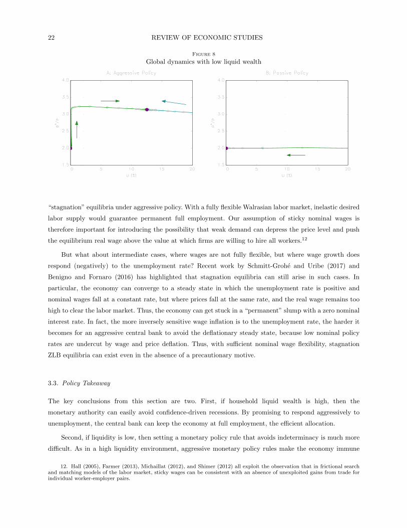
3.2.3. Global Dynamics. To conclude the analysis, in Figure 8 we numerically explore the global
equilibrium dynamics, including real house price dynamics, that arise in the low liquid wealth case.11 The left
panel displays possible equilibria in the case of aggressive monetary policy. There are no paths converging to
full employment in this case, but there are equilibrium paths converging to the stagnation steady state. The
path converging from the left displays some interesting features. In the initial phase of the equilibrium path
(the vertical part), unemployment is low and nearly constant but house prices are gradually increasing. To
an outside observer, the economy would appear to be experiencing a house price bubble: a steadily increasing
price with no change in fundamentals. What sustains this “bubble-like” path as an equilibrium outcome is
the fact that in the long run, agents expect the economy will converge to the stagnation steady state with
permanent unemployment, and here house prices will remain relatively high because they will have a high
value as a source of liquidity.
The right panel instead depicts the equilibrium paths that arise under passive monetary policy. Recall
that in this parameterization (corresponding to Figure 7), policy is sufficiently passive that the model has a
unique steady state at full employment. The path plotted represents equilibria in which unemployment starts
out positive, but gradually declines to zero. Note that if an unexpected sunspot shock were to cause the
economy to jump from full employment to a point on this path, one would observe a jump in unemployment,
but little change in house prices. This is possible because when unemployment is temporarily high, the
fundamental value of housing is low and the liquidity value is high, while this decomposition is gradually
reversed as unemployment declines. We explore such a scenario more fully below when we use the model to
construct a narrative for the Great Recession in the United States.
3.2.4. Alternative Models of Wage Stickiness. At this point it seems important to discuss
the importance of our assumption of exogenous nominal wage growth (i.e., wage stickiness) in generating
11. We use the same parameter values used to plot Figure 7. The arrows indicate the direction of the equilibrium path,and the circles along the stable manifolds are one model period apart.
22 REVIEW OF ECONOMIC STUDIES
Figure 8
Global dynamics with low liquid wealth
“stagnation” equilibria under aggressive policy. With a fully flexible Walrasian labor market, inelastic desired
labor supply would guarantee permanent full employment. Our assumption of sticky nominal wages is
therefore important for introducing the possibility that weak demand can depress the price level and push
the equilibrium real wage above the value at which firms are willing to hire all workers.12
But what about intermediate cases, where wages are not fully flexible, but where wage growth does
respond (negatively) to the unemployment rate? Recent work by Schmitt-Grohe and Uribe (2017) and
Benigno and Fornaro (2016) has highlighted that stagnation equilibria can still arise in such cases. In
particular, the economy can converge to a steady state in which the unemployment rate is positive and
nominal wages fall at a constant rate, but where prices fall at the same rate, and the real wage remains too
high to clear the labor market. Thus, the economy can get stuck in a “permanent” slump with a zero nominal
interest rate. In fact, the more inversely sensitive wage inflation is to the unemployment rate, the harder it
becomes for an aggressive central bank to avoid the deflationary steady state, because low nominal policy
rates are undercut by wage and price deflation. Thus, with sufficient nominal wage flexibility, stagnation
ZLB equilibria can exist even in the absence of a precautionary motive.
3.3. Policy Takeaway
The key conclusions from this section are two. First, if household liquid wealth is high, then the
monetary authority can easily avoid confidence-driven recessions. By promising to respond aggressively to
unemployment, the central bank can keep the economy at full employment, the efficient allocation.
Second, if liquidity is low, then setting a monetary policy rule that avoids indeterminacy is much more
difficult. As in a high liquidity environment, aggressive monetary policy rules make the economy immune
12. Hall (2005), Farmer (2013), Michaillat (2012), and Shimer (2012) all exploit the observation that in frictional searchand matching models of the labor market, sticky wages can be consistent with an absence of unexploited gains from trade forindividual worker-employer pairs.

HEATHCOTE & PERRI WEALTH & VOLATILITY 23
to sunspot shocks that generate temporary fluctuations around the full employment steady state. However,
the fact that in the low liquid wealth case the model has multiple steady states (Result 7) indicates that
an aggressive monetary policy cannot avoid sunspot shocks that set the economy on paths leading to a
permanent slump.
In contrast, a passive policy rule, while it renders the economy vulnerable to sunspot shocks around
full employment, has the advantage that it can rule out permanent slumps. The idea is that in a permanent
slump, households have a strong precautionary motive, and thus a low interest rate is required to support
demand equal to constant expected output. If monetary policy is sufficiently passive, interest rates will never
fall low enough, and thus markets can clear with positive unemployment only if the economy is expected to
gradually recover.13
So what should the monetary authority do in a low liquid wealth environment? No simple rule in the
class we have considered guarantees that the economy will remain glued to full employment. Recent work
in related models has shown that multiplicity can be eliminated if the monetary authority commits to a
policy that switches from an interest rate rule to a money rule when the economy heads toward the ZLB
steady state (see Benhabib et al., 2002 and Atkeson, Chari, and Kehoe, 2010). Our setup is different in
that multiplicity is due to expectations about high unemployment rather than expectations of a deflationary
spiral. Nonetheless, the fact that high liquid wealth ensures that the ZLB equilibrium does not exist (see
Result 6) suggests that an aggressive interest rate policy coupled with a commitment to liquidity creation
in the event that the economy should ever head toward the ZLB steady state might restore uniqueness.
Exploring this conjecture formally is an interesting future research direction. In Section 5. below we will
explore the role for non-monetary macroeconomic stabilization tools.
4. APPLICATION: THE GREAT RECESSION
The dashed lines in Figure 9 show time paths for (i) the unemployment rate, (ii) house prices, (iii) inflation,
and (iv) the federal funds rate in the United States between 2006 and 2016. The house price series plotted is
the Case-Shiller U.S. National Home Price Index, deflated by the GDP deflator, and relative to a 2% trend
growth rate for the real price.14 Between the start of 2007 and the end of 2008, house prices fell by 30%
relative to trend, largely accounting for the sharp fall in median net worth documented in Figure 1. The rise
in the unemployment rate was concentrated in the second half of 2008 and the first half of 2009. Thus, the
fall in house prices began well before the most severe portion of the recession.
Although our model is highly stylized, we would like to know whether it can replicate these features
of the U.S. Great Recession. In particular, we are interested in constructing and comparing to data an
equilibrium path in which a sunspot shock, in the context of a low liquid wealth and passive monetary policy
13. The point that sticking to a high interest rate policy can rule out permanent slumps is sometimes labeled the “Neo-Fisherian” channel of monetary policy. It has been advocated, among others, by Schmitt-Grohe and Uribe (2017). In our modela passive policy works because high interest rates are inconsistent with expectations of permanently depressed output. InSchmitt-Grohe and Uribe the policy works because high interest rates are inconsistent with expectations of permanently lowinflation.
14. This is the average growth rate for real GDP per capita between 1947 and 2007. It is also close to the average growthrate for real house prices between 1975 and 2006 (see Figure 1 in Davis and Heathcote, 2007).
24 REVIEW OF ECONOMIC STUDIES
environment, triggers a jump in unemployment followed by a gradual perfect foresight recovery. This exercise
requires picking values for the model parameters.
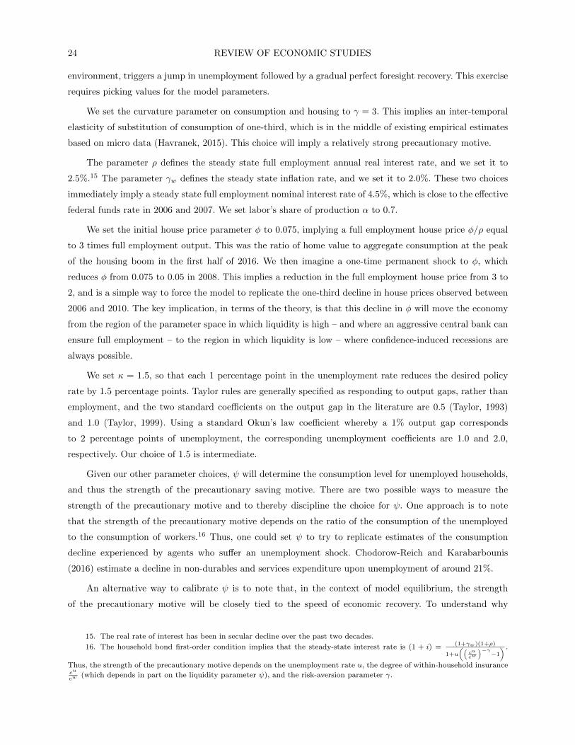
We set the curvature parameter on consumption and housing to γ = 3. This implies an inter-temporal
elasticity of substitution of consumption of one-third, which is in the middle of existing empirical estimates
based on micro data (Havranek, 2015). This choice will imply a relatively strong precautionary motive.
The parameter ρ defines the steady state full employment annual real interest rate, and we set it to
2.5%.15 The parameter γw defines the steady state inflation rate, and we set it to 2.0%. These two choices
immediately imply a steady state full employment nominal interest rate of 4.5%, which is close to the effective
federal funds rate in 2006 and 2007. We set labor’s share of production α to 0.7.
We set the initial house price parameter φ to 0.075, implying a full employment house price φ/ρ equal
to 3 times full employment output. This was the ratio of home value to aggregate consumption at the peak
of the housing boom in the first half of 2016. We then imagine a one-time permanent shock to φ, which
reduces φ from 0.075 to 0.05 in 2008. This implies a reduction in the full employment house price from 3 to
2, and is a simple way to force the model to replicate the one-third decline in house prices observed between
2006 and 2010. The key implication, in terms of the theory, is that this decline in φ will move the economy
from the region of the parameter space in which liquidity is high – and where an aggressive central bank can
ensure full employment – to the region in which liquidity is low – where confidence-induced recessions are
always possible.
We set κ = 1.5, so that each 1 percentage point in the unemployment rate reduces the desired policy
rate by 1.5 percentage points. Taylor rules are generally specified as responding to output gaps, rather than
employment, and the two standard coefficients on the output gap in the literature are 0.5 (Taylor, 1993)
and 1.0 (Taylor, 1999). Using a standard Okun’s law coefficient whereby a 1% output gap corresponds
to 2 percentage points of unemployment, the corresponding unemployment coefficients are 1.0 and 2.0,
respectively. Our choice of 1.5 is intermediate.
Given our other parameter choices, ψ will determine the consumption level for unemployed households,
and thus the strength of the precautionary saving motive. There are two possible ways to measure the
strength of the precautionary motive and to thereby discipline the choice for ψ. One approach is to note
that the strength of the precautionary motive depends on the ratio of the consumption of the unemployed
to the consumption of workers.16 Thus, one could set ψ to try to replicate estimates of the consumption
decline experienced by agents who suffer an unemployment shock. Chodorow-Reich and Karabarbounis
(2016) estimate a decline in non-durables and services expenditure upon unemployment of around 21%.
An alternative way to calibrate ψ is to note that, in the context of model equilibrium, the strength
of the precautionary motive will be closely tied to the speed of economic recovery. To understand why
15. The real rate of interest has been in secular decline over the past two decades.
16. The household bond first-order condition implies that the steady-state interest rate is (1 + i) =(1+γw)(1+ρ)
1+u
((cu
cw
)−γ−1
) .Thus, the strength of the precautionary motive depends on the unemployment rate u, the degree of within-household insurancecu
cw(which depends in part on the liquidity parameter ψ), and the risk-aversion parameter γ.
HEATHCOTE & PERRI WEALTH & VOLATILITY 25
this is the case, note first that we will calibrate the sunspot shock to generate a realistic increase in the
unemployment rate at the start of the recession. In equilibrium, a given increase in unemployment must
induce a commensurate decline in desired consumer spending. This reduction in demand can be obtained
in different ways. If consumers have a strong precautionary motive (small ψ), even a short-lived increase in
unemployment (i.e. a fast expected recovery) is sufficient to support the required fall in demand. Alternatively,
if consumers have a weaker precautionary motive (larger ψ) then they will only want to reduce spending
by the same amount if they expect a slower recovery and thus lower permanent income. Thus, for a fixed
increase in unemployment (given by the data) a larger ψ (a weaker precautionary motive) will correspond
to a slower equilibrium expected recovery.
The fact that estimated empirical consumption declines upon unemployment are quite small points
towards a relatively large value for ψ, as does the fact that the observed post-recession recovery in the
United States was very slow. At the same time, however, in order to construct an equilibrium in which a
recovery to full employment is even possible, monetary policy must be passive (Result 5). Given our other
parameter values –and in particular the choice for κ– this imposes an upper bound on ψ equal to 0.37.17
Intuitively, ψ > 0.37 would imply such a weak precautionary motive that even if agents were to expect
permanent stagnation they would still not reduce demand sufficiently to validate a marginal increase in
unemployment.
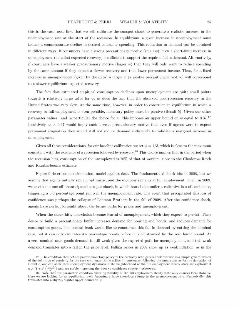
Given all these considerations, for our baseline calibration we set ψ = 1/3, which is close to the maximum
consistent with the existence of a recession followed by recovery.18 This choice implies that in the period when
the recession hits, consumption of the unemployed is 76% of that of workers, close to the Chodorow-Reich
and Karabarbounis estimate.
Figure 9 describes our simulation, model against data. The fundamental φ shock hits in 2008, but we
assume that agents initially remain optimistic, and the economy remains at full employment. Then, in 2009,
we envision a one-off unanticipated sunspot shock, in which households suffer a collective loss of confidence,
triggering a 6.0 percentage point jump in the unemployment rate. The event that precipitated this loss of
confidence was perhaps the collapse of Lehman Brothers in the fall of 2008. After the confidence shock,
agents have perfect foresight about the future paths for prices and unemployment.
When the shock hits, households become fearful of unemployment, which they expect to persist. Their
desire to build a precautionary buffer increases demand for housing and bonds, and reduces demand for
consumption goods. The central bank would like to counteract this fall in demand by cutting the nominal
rate, but it can only cut rates 4.5 percentage points before it is constrained by the zero lower bound. At
a zero nominal rate, goods demand is still weak given the expected path for unemployment, and this weak
demand translates into a fall in the price level. Falling prices in 2009 show up as weak inflation, as in the
17. The condition that defines passive monetary policy in the economy with general risk aversion is a simple generalizationof the definition of passivity for the case with logarithmic utility. In particular, following the same steps as for the derivation ofResult 5, one can show that unemployment dynamics in the neighborhood of the full employment steady state are explosive if
κ > (1 + ρ)(
1−λγλγ
)and are stable – opening the door to confidence shocks – otherwise.
18. Note that our parametric condition ensuring stability of the full employment steady state only ensures local stability.Here we are looking for an equilibrium path featuring a large (non-local) jump in the unemployment rate. Numerically, thistranslates into a slightly tighter upper bound on ψ.
26 REVIEW OF ECONOMIC STUDIES
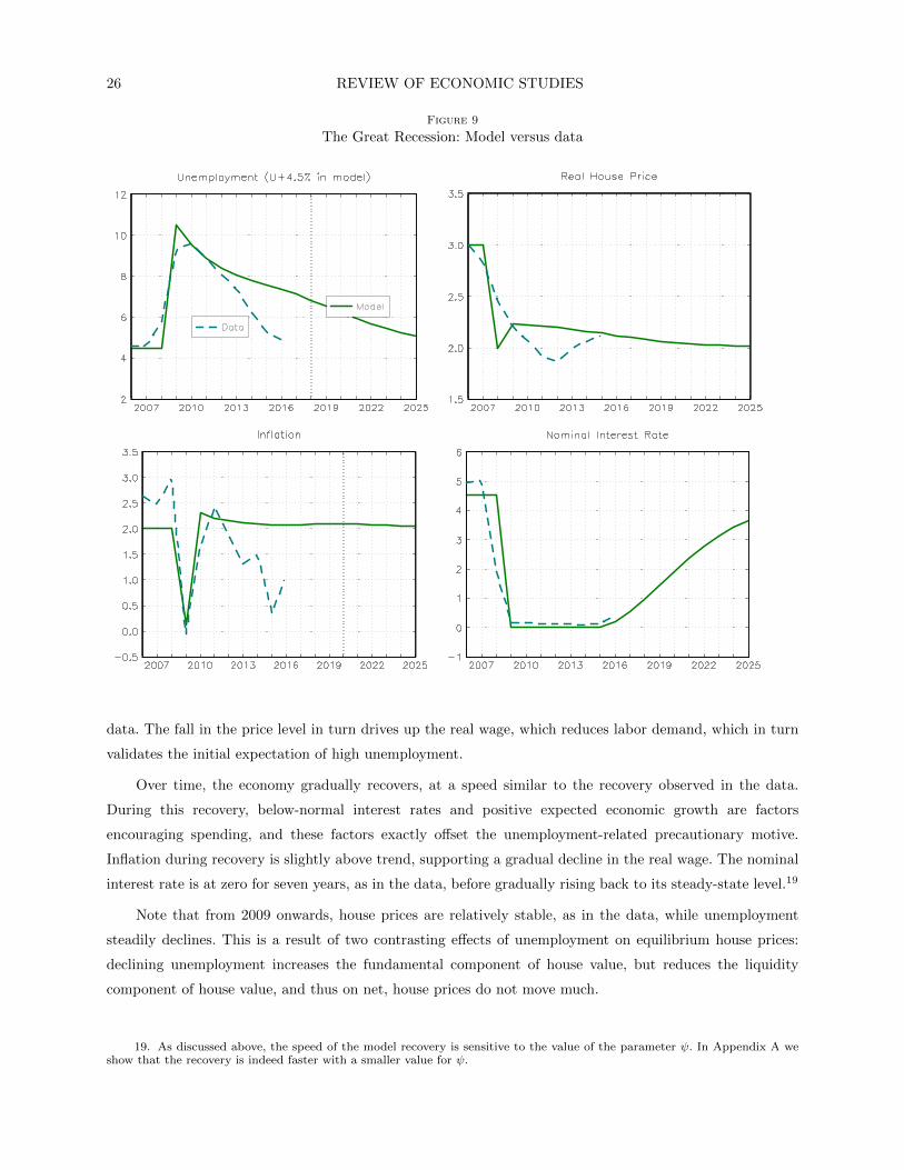
Figure 9
The Great Recession: Model versus data
data. The fall in the price level in turn drives up the real wage, which reduces labor demand, which in turn
validates the initial expectation of high unemployment.
Over time, the economy gradually recovers, at a speed similar to the recovery observed in the data.
During this recovery, below-normal interest rates and positive expected economic growth are factors
encouraging spending, and these factors exactly offset the unemployment-related precautionary motive.
Inflation during recovery is slightly above trend, supporting a gradual decline in the real wage. The nominal
interest rate is at zero for seven years, as in the data, before gradually rising back to its steady-state level.19
Note that from 2009 onwards, house prices are relatively stable, as in the data, while unemployment
steadily declines. This is a result of two contrasting effects of unemployment on equilibrium house prices:
declining unemployment increases the fundamental component of house value, but reduces the liquidity
component of house value, and thus on net, house prices do not move much.
19. As discussed above, the speed of the model recovery is sensitive to the value of the parameter ψ. In Appendix A weshow that the recovery is indeed faster with a smaller value for ψ.

HEATHCOTE & PERRI WEALTH & VOLATILITY 27
Overall, we take this exercise as providing suggestive evidence that a sudden loss of confidence in a
low liquid wealth environment played a quantitatively important role in generating the Great Recession and
subsequent slow recovery in the United States.
5. POLICY
We now show how a simple unemployment insurance (UI) scheme can be used to increase within-household
insurance, and thereby help to rule out the possibility of confidence-driven fluctuations.
We assume that the government can implement a UI scheme in which it taxes workers lump-sum a
nominal amount Tt and immediately transfers the resources raised to the unemployed in the form of a
constant amount of consumption b. The budget constraint for this policy is
(1− ut)Tt = utptb.
Such a policy redistributes from low marginal utility workers to high marginal utility unemployed workers –
precisely the reallocation that households cannot achieve when liquid wealth is low – and thereby dampens
households’ precautionary motive to save. Thus, the UI scheme will shift up the i(u) function in Figure 5
and – because it reduces the liquidity value of housing wealth – shift down the house price function in Figure
4 (in this sense, public insurance crowds out private insurance). With a sufficiently generous UI policy, the
government will be able to ensure that the i(u) function lies above zero for all u, effectively shifting the
economy from a low liquid wealth regime to a high liquid wealth regime. In the calibration described in our
Great Recession application, a value of b = 0.29 (i.e., unemployment benefits are 29% of full employment
output) is sufficient to achieve this. Thus, unemployment insurance and monetary policy are complementary
policy tools when liquid wealth is low: UI effectively provides a substitute for low liquid private wealth, and
an aggressive monetary policy can then be used to eliminate confidence-driven fluctuations.
There is a literature exploring how redistributive policies can be used to counter a negative aggregate
shock to the economy, for example by redistributing income from households with a low marginal propensity
to consume to those with a high MPC (see, for example, Kekre, 2017, or McKay and Reis, 2016). The element
that is different here is that redistributive policies can work in our model by preventing a negative aggregate
shock from emerging in the first place, by dampening the feedback loop from pessimistic expectations to
weak demand, and thereby ruling out self-fulfilling expectations-driven fluctuations. Thus, redistribution is
valuable as an ex ante policy that narrows the set of shocks that can arise in equilibrium, rather than as an
ex post policy response to mitigate the response to exogenously given shocks.
Note, however, that our simple model stacks the deck in favor of introducing public insurance because
it exogenously assumes zero private unemployment insurance, while allowing for any amount of non-
distortionary public insurance. A more satisfactory theory of optimal public insurance would model both
the frictions that create a role for public insurance in the first place, as well as the disincentives to search
and work effort associated with public taxes and transfers. However, one finding that is likely to generalize
is that public policies that increase insurance against idiosyncratic risk are especially valuable at times when

28 REVIEW OF ECONOMIC STUDIES
(i) a strong precautionary motive is restraining aggregate demand and (ii) monetary policy is constrained
by the zero lower bound.
6. MICROECONOMIC EVIDENCE
A key element of our model is that when households have low liquid wealth, their desired saving rate becomes
more sensitive to perceived unemployment risk. When unemployment risk rises, wealth-poor households’
desire to save becomes much stronger, which translates into lower equilibrium employment, and rationalizes
ex post the fear of high unemployment. Is this mechanism empirically relevant for understanding the decline
in aggregate consumption during the Great Recession?
We cannot easily test this mechanism in aggregate time series. But at the household level there is
significant heterogeneity in wealth. In this section we will exploit this heterogeneity to explore whether
low-wealth households increased their saving by more than high-wealth households in response to rising
unemployment risk during the Great Recession. We also investigate alternative potential drivers of differential
saving rates between low- and high-wealth groups, such as differential wealth losses, future income prospects,
or unemployment risk.
We start by documenting novel evidence, based on data from the Consumer Expenditure Survey (CES)
and the Panel Study of Income Dynamics (PSID), that at the onset of the recession lower wealth households
exhibit systematically larger increases in their saving rates. This evidence is broadly consistent with a number
of empirical studies showing that wealth is an important determinant of consumption responses to income
shocks (see Section 1.1). Collectively, this evidence lends support to the importance of wealth and the
precautionary motive in understanding demand dynamics.
6.1. Rich and Poor
Before contrasting savings across wealth groups, we first verified that the dynamics of aggregate consumption,
income, and wealth in our cross sectional data capture the broad contours of national income and product
accounts (NIPA) aggregates over the course of the Great Recession (see Appendix C for details). The sample
we select for our analysis includes all households in the PSID and the CES with a head or spouse between ages
22 and 60, and which report income and consumption for at least two consecutive interviews over the period
2004-2013. We focus on households of working age, since unemployment risk is most relevant for this group.
For each data set and for each year t, we split households by wealth into two equal-sized groups: “rich” and
“poor”. In constructing our wealth ranking, we measure wealth as net worth in period t relative to a measure
of consumption expenditure around period t. We focus on net worth relative to consumption (as opposed to
just net worth) as this ratio better captures the extent to which a household can shield consumption from
income declines, and is thus more closely connected to the strength of households’ precautionary motive.20
20. See Appendix C for the details on how we define these cutoffs in both the CES and the PSID. The appendix alsoshows that our results are robust to using net worth (not normalized by consumption expenditures) to define the rich-poorsample split.

HEATHCOTE & PERRI WEALTH & VOLATILITY 29
TABLE 1
Characteristics of rich and poor, 2006
PSID CESPoor Rich All Poor Rich All
Sample size (unweighted) 3,443 2,508 5,951 1,915 1,960 3,875
Mean age of head38.0
(0.32)
47.1(0.26)
42.5(0.19)
40.2(0.25)
46.4(0.24)
43.3(0.16)
Head with college (%)20.5(1.0)
36.6(1.0)
28.6(0.8)
24.8(1.1)
39.4(1.2)
32.1(0.7)
Mean household size2.47
(0.04)
2.73(0.04)
2.60(0.02)
2.79(0.04)
2.85(0.04)
2.82(0.02)
Mean household net worth ($)12,017
(964)
619,831(49,297)
315,997(30,634)
11,967(1,155)
338,535(12,644)
175,259(7,450)
Median household net worth ($)5,000(506)
265,000(6,789)
66,000(3,006)
1,800(294)
187,102(4,893)
58,765(2,222)
Per capita disp. income ($)14,951
(265)
28,476(728)
22,052(433)
18,739(334)
30,184(593)
24,401(385)
Head unemployment rate (%)4.2
(0.36)
1.0(0.19)
2.5(0.2)
1.0(0.3)
0.3(0.2)
0.6(0.1)
Per capita cons. expenditure ($)9,832(186)
13,101(244)
11,548(170)
9,185(232)
10,858(188)
10,013(166)
Saving rate (%)34.2
(0.90)
54.0(0.95)
47.6(0.75)
51.0(1.18)
64.0(0.66)
59.0(0.59)
Notes: Bootstrapped standard errors in parentheses. All statistics (except sample size) weighted using sample weights
6.1.1. Summary Statistics. Table 1 reports, for the year 2006, characteristics of the rich and poor
groups in both the PSID and the CES.
Although the levels of many of these statistics differ across data sets (due in part to different coverage,
sample design, and exact question asked), differences between rich and poor are comparable across the two
data sets. With respect to demographics, the wealth-poor group is younger and less educated. The most
striking difference between the two groups, not surprisingly, is in terms of wealth. Median net worth for the
poor group is near zero in both surveys, while for the rich group it is around $265,000 in the PSID and
around $187,000 in the CES.21 This dramatic difference suggests that the precautionary saving motive for
the poor group should be much stronger than for the rich group, while the rich group likely experiences much
larger capital losses when housing and stock prices fall.
The wealth-poor group also has a higher (pre-recession) unemployment rate and has a little more than
half the average income of the rich group. At the same time, the poor group has a much lower saving rate,
so that differences in consumption expenditures between the two groups are relatively small (around 20%
21. One reason for the difference between the two data sets is that the measure of net worth in the PSID includes moreassets, such as individual retirement accounts, vehicles, and family businesses. See Appendix C for details.

30 REVIEW OF ECONOMIC STUDIES
in the CES and 30% in the PSID).22 Overall the table suggests that the two groups are quite different in
nature for a variety of reasons. This is why our interest is not in the levels of their respective saving rates,
but rather in how their saving rates change differentially at the onset of the Great Recession, when the labor
income risk faced by both groups increases dramatically.
6.1.2. Changes in Saving Rates. We now compute the object of interest: changes over time in
the saving rates of households in different groups of the net worth distribution. It is important that the set
of households in each wealth group is fixed when we measure the change in the saving rate between two
successive periods, so that the change in the measured saving rate reflects a true change in household savings
behavior, and is not a result of a change in the composition of the groups. Fortunately, both the PSID and
CES data sets have a panel dimension: in the PSID, households are re-interviewed every two years, while in
the CES they are interviewed for four consecutive quarters, and in their first and last interviews, they report
both income and consumption. Let i denote a group of households (say, households with wealth below the
median in 2006) and t t+ 1 denote a time interval (say, 2006-2008). The change in group i’s saving rate over
the interval t t+ 1, ∆sit t+1, is computed as
∆si,t t+1 =E(Yi,t+1)− E(Ci,t+1)
E(Yi,t+1)− E(Yi,t)− E(Ci,t)
E(Yi,t), (6.18)
where Y denotes household disposable income, C denotes household consumption expenditures, and E
denotes the group average (see Appendix C for more details).
Figure 10 plots changes in saving rates computed from the PSID (top panels) and from the CES (bottom
panels). The two panels on the left (A and C) show the evolution over time of the changes in saving rates
of the rich and poor groups. Both panels show that in “normal” times, there are no significant differences in
saving rate changes between the two wealth groups, while at the onset of the Great Recession wealth-poor
households increased their saving rate significantly more than wealth-rich households.23
The two panels on the right (B and D) disaggregate more finely by net worth, and report the changes
in saving rates for the five quintiles of the net worth distribution. Here we focus on just two time periods: a
pre-recession period, and the period when the economy enters recession. The plots show that as the economy
moves into recession, saving rates increase for all wealth quintiles, but the increase in the saving rate is a
declining function of initial net worth, with the bottom quintiles increasing their saving rates significantly,
while the top quintiles experience much smaller increases.
The fact that during the Great Recession poor households increased their saving rates much more than
the rich points towards an important precautionary motive in the face of rising unemployment risk. However,
there are other potential explanations for this especially sharp increase in the saving rate of the poor. In
22. The level of the unemployment rate is quite different across the two surveys, with the CES having a much lowerrate. The reason is that unemployment in the PSID is computed (more accurately) as the ratio of weeks (in the relevant year)reported as unemployed to the total weeks reported as working or unemployed. In the CES, in contrast, the unemploymentrate is the ratio of heads who reported being unemployed for the full year to the ratio of heads who reported either working orbeing full year unemployed.
23. Saving rate declines in the CES appear to be smaller than in the PSID. We conjecture that this reflects the fact thatthe CES saving rate changes are computed over nine-month intervals and based on quarterly consumption figures, while thePSID changes are recorded over two-year intervals and based on annual consumption figures.

HEATHCOTE & PERRI WEALTH & VOLATILITY 31
Figure 10
Changes in saving rates for rich and poor
-4
-2
0
2
4
6
8
10
12
2004-2006 2006-2008 2008-2010 2010-2012
Cha
nge
in s
avin
g ra
te (p
p)
A. PSID over time
Rich
Poor
-4
-2
0
2
4
6
8
10
12
Q1 Q2 Q3 Q4 Q5
2004-2006
2006-2008
B. PSID by Net Worth Quintile
-1
0
1
2
3
4
2005-06 2006-07 2007-08 2008-09 2009-10 2010-11 2011-12 2012-13
Cha
nge
in s
avin
g ra
te (p
p)
C. CES over time
Rich
Poor
Note: the thin dashed lines delimit bootstrapped 2 standard error bands.
Years
-1
0
1
2
3
4
Q1 Q2 Q3 Q4 Q5Net Worth Quintiles
2004-2006
2006-2008
D. CES by Net Worth Quintile
particular, it is possible that the poor were more adversely affected by deteriorating future income prospects,
by rising unemployment, or by falling asset values. In order to control for these alternative explanations for
the observed increase in saving, we make use of the long panel nature of the PSID. Having a long panel
is important as it allows us to assess whether the change in saving during the recession is related to these
post-recession outcomes. For this exercise, we select all the households that are in the sample continuously
from 2004 through 2012 and that satisfy the age restrictions specified above. This leaves us with a sample
of 3,773 households, which we then divide into rich and poor groups using as a cutoff (weighted) net worth
at the end of 2006 (relative to average consumption expenditures over the period 2006-2008).
In Figure 11 we track the evolution of several variables for these two groups over time. Panel A reports
saving rates, and confirms the findings of Figure 10: as the recession hits, both groups increased their saving
rates, but the poor increased saving much more than the rich. Panels B and C report the paths for the
two components of the saving rate: disposable income and consumption expenditures. Over the period 2008-
2012, disposable income growth of both rich and poor slows down, but it is the income of the rich that
slows more during and after the recession. This suggests that the disproportionate increase in saving of the
poor cannot be attributed to their expecting relatively weak future income growth. Panel D shows that

32 REVIEW OF ECONOMIC STUDIES
Figure 11
Rich and poor: a long panel analysis
-.04
-.02
.00
.02
.04
.06
.08
.10
.12
2004 2006 2008 2010 2012
Cha
nge
from
200
6 sa
ving
rate
(pp)
A. Saving Rates
Rich
Poor
0.90
0.95
1.00
1.05
1.10
1.15
1.20
1.25
1.30
2004 2006 2008 2010 2012
Rat
io to
200
6 In
com
e
B. Disposable Income
Rich
Diff
eren
ce fr
om 2
006
rate
(pp)
0.90
0.95
1.00
1.05
1.10
1.15
1.20
1.25
1.30
2004 2006 2008 2010 2012
Rat
io to
200
6 ex
pend
iture
s
C. Consumption Expenditures
Rich
Poor
Poor
Poor
Diff
eren
ce fr
om 2
006
ratio
(pp)
Rich
0.0
0.5
1.0
1.5
2.0
2.5
3.0
3.5
2004 2006 2008 2010 2012
D. Unemployment Rate
Rich
Poor
-250
-200
-150
-100
-50
0
50
100
2004 2006 2008 2010 2012
E. Net Worth to Income Ratio
during and after the recession, both groups faced similar increases in unemployment risk, suggesting that
differential unemployment risk cannot explain why the poor increased their saving rate more.24 Panel C
shows that consumption growth of the rich declines more than consumption of the poor. This is consistent
with the evidence presented in Petev, Pistaferri, and Saporta-Eksten (2011) that high-wealth households
reduced consumption expenditures the most during the recession, and it is also consistent with Parker and
Vissing-Jorgensen (2009), who show that in recent recessions, consumption expenditures of high-income
households have been more cyclical than those of low-income households. Note, however, that while the rich
group chooses a somewhat larger reduction in consumption, they also face a much larger slowdown in income,
so that their saving rate does not increase as much as the saving rate of the poor. Finally, panel E shows the
24. The evidence in panels B and D is also consistent with De Nardi, French, and Benson (2012). They show that duringthe 2009 recession, high-income and high-education households were more pessimistic about their income prospects relative totheir poorer and less-educated counterparts.

HEATHCOTE & PERRI WEALTH & VOLATILITY 33
path of wealth as a fraction of disposable income. Note that, relative to 2006, net worth of the rich declines
by over 100% of their disposable income, while the poor actually experience an increase in net worth. Thus,
the larger increase in saving by the poor cannot be attributed to the poor having experienced larger wealth
losses during the recession. Note also that households in the poor group increase their net worth by around
50% of their income during the recession. This finding provides independent evidence that this group really
is increasing saving. In addition, the net worth data confirm the popular narrative of deleveraging during the
Great Recession: low-wealth households cut expenditure to reduce debts and rebuild eroded balance sheets.
Overall, the evidence from the panel analysis in Figure 11 supports our hypothesis that the differential
changes in saving rates shown in Figure 10 reflect a strong precautionary motive to save on the part of
wealth-poor households in the face of rising unemployment risk. The magnitudes of the observed changes in
saving rates are economically relevant. For example, in the PSID over the period 2006-2008, poor households
increased their saving rate by about 4 percentage points more than rich households. If we attribute this
difference to a stronger precautionary motive, then given that the poor account for about one-third of total
disposable income (see Table 1), we can conclude that increased precautionary saving by the poor reduced
aggregate consumption by 1/3× 4% ' 1.3% of aggregate disposable income.
7. CONCLUSIONS
The message of this paper is that when household wealth is low, a decline in consumer confidence can be
self-fulfilling because with low wealth, higher unemployment risk implies a large increase in the precautionary
motive to save, rationalizing low equilibrium consumption and output. We argued that the decline in U.S.
house prices in 2007 and 2008 reduced U.S. household net worth and left the U.S. economy vulnerable to
just such a self-fulfilling wave of pessimism.
We developed a simple model to explore the conditions under which confidence-driven fluctuations are
possible and to illustrate the connections between the level of liquid wealth, the monetary policy rule, and
the nature of confidence-driven fluctuations that can arise. Precautionary motives that vary with wealth and
unemployment risk play the key role in these links. These precautionary motives are central in standard
inter-temporal consumption theory and are consistent with consumption patterns observed in micro data
during the course of the Great Recession.
An obvious project for future work is to develop a richer, more quantitative version of the model. One
interesting extension would be to introduce household heterogeneity in net worth, to better understand the
implications for aggregate precautionary demand of the extremely uneven distribution of net worth in the
United States. A richer model of labor markets, in which desired labor supply plays a role in the long-run
adjustment process, is another direction for future research. Finally, it would be interesting to introduce
capital in the environment, since an increase in perceived unemployment risk would both increase the supply
of saving and reduce the demand for investment, thereby changing the contours of the macroeconomic
response.
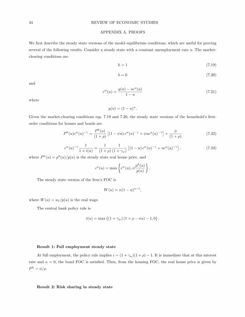
34 REVIEW OF ECONOMIC STUDIES
APPENDIX A. PROOFS
We first describe the steady state versions of the model equilibrium conditions, which are useful for proving
several of the following results. Consider a steady state with a constant unemployment rate u. The market-
clearing conditions are
h = 1 (7.19)
b = 0 (7.20)
and
cw(u) =y(u)− ucu(u)
1− u(7.21)
where
y(u) = (1− u)α.
Given the market-clearing conditions eqs. 7.19 and 7.20, the steady state versions of the household’s first-
order conditions for houses and bonds are
Ph(u)cw(u)−γ =Ph(u)
(1 + ρ)
[(1− ψu) cw(u)−γ + ψucu(u)−γ
]+
φ
(1 + ρ)(7.22)
cw(u)−γ1
1 + i(u)=
1
(1 + ρ)
1
(1 + γw)
[(1− u) cw(u)−γ + ucu(u)−γ
], (7.23)
where Ph(u) = ph(u)/p(u) is the steady state real house price, and
cu(u) = max
{cw(u), ψ
ph(u)
p(u)
}.
The steady state version of the firm’s FOC is
W (u) = α(1− u)α−1,
where W (u) = wt/p(u) is the real wage.
The central bank policy rule is
i(u) = max {(1 + γw) (1 + ρ− κu)− 1, 0} .
Result 1: Full employment steady state
At full employment, the policy rule implies i = (1 + γw)(1 + ρ)− 1. It is immediate that at this interest
rate and u = 0, the bond FOC is satisfied. Then, from the housing FOC, the real house price is given by
Ph = φ/ρ.
Result 2: Risk sharing in steady state

HEATHCOTE & PERRI WEALTH & VOLATILITY 35
To prove that if risk sharing is perfect then λ ≥ 1, note that with perfect risk sharing the real house
price equals the present value of implicit rents, Ph = φy/ρ. A necessary condition for risk sharing to be
perfect is that the value of liquid wealth has to be at least as high as per capita output, i.e.,
ψPh ≥ y.
Substituting in the expression for Ph yields
λ ≡ ψφ/ρ ≥ 1.
We now prove, by contradiction, that if λ ≥ 1, then risk sharing is perfect. Assume that λ ≥ 1 and that
risk sharing is imperfect. If risk sharing is imperfect, then the real price of housing (using Result 3 below) is
Ph =φ
ρy
u+ φ
λu+ (1 + (λ− 1)u)φ.
In addition, a necessary condition for risk sharing to be imperfect is ψPh < y. Substituting in this
inequality, the expression for Ph yields
λu+ φ
λu+ (1 + (λ− 1)u)φ< 1,
which simplifies to
u > 1,
which is impossible, thus contradicting the assumption of imperfect risk sharing.
Result 3: Steady-state house prices with imperfect risk sharing
Assuming imperfect risk sharing,
cu(u) = ψPh(u). (7.24)
Imposing γ = 1 (logarithmic utility), the steady state house price eq. 7.22 can then be written as
Ph(u)
cw(u)=
φ+ u
ρ+ ψu.
Spending by workers, using 7.21, is
cw(u) =(1− u)α − uψPh(u)
1− u. (7.25)
Substituting this into the previous equation, one can solve out for Ph(u) :
Ph(u) =φ
ρ(1− u)α
u+ φ
ψφρ u+
(1 +
(ψφρ − 1
)u)φ
=φ
ρ(1− u)α
u+ φ
λu+ (1 + (λ− 1)u)φ.

36 REVIEW OF ECONOMIC STUDIES
Result 4: Steady-state interest rates
The steady state version of the bond first-order condition can be written, after substituting in market-
clearing conditions, as
1
cw1
1 + i(u)=
1
1 + ρ
1
1 + γw
(1− ucw
+u
cu
)1
1 + i(u)=
1
1 + ρ
1
1 + γw
((1− u) + u
cw
cu
).
Now substitute in 7.25 and 7.24:
1
1 + i(u)=
1
1 + ρ
1
1 + γw
(1− u) +u (1−u)α−uψPh(u)
1−uψPh
. (7.26)
Subsituting in eq. 7.22 gives the expression in the text:
1 + i(u) = (1 + ρ) (1 + γw)
u+ φ
u(
1 + ρψ − φ
)+ φ
. (7.27)
It is immediate to show that if u = 0, then 1 + i(u) = (1 + ρ)(1 + γw). Differentiating eq. 7.27 with
respect to u, it is straightforward to show that the equilibrium interest rate i(u) is declining in u given λ < 1.
Similarly, λ < 1 ensures that the second derivative of i(u) with respect to u is positive, so i(u) is a convex
function of u.
Result 5: Monetary policy and stability of steady states
If monetary policy is aggressive, then the full employment steady state is locally unstable, in the sense
that there are no perfect foresight equilibrium paths that converge to this steady state in which the initial
unemployment rate is positive. If monetary policy is passive, then the full employment steady state is stable,
and sunspot shocks are possible.
Assuming perfect foresight, the first-order condition for bonds can be written as
1
cwt
1 + ρ
1 + it=
1pt+1
pt
[1− ut+1
cwt+1
+ut+1
cut
],
where Pht is the real house price. From the firm’s first-order condition,
pt+1
pt=
(1 + γw)(1− ut+1)(1−α)
(1− ut)(1−α).
Assuming the unemployed are borrowing constrained and imposing market clearing, we have
cut = ψPht+1
cwt = (1− ut)α−1 −ut
1− utψPht .
HEATHCOTE & PERRI WEALTH & VOLATILITY 37
Finally, the policy rule (assuming the ZLB is not binding) is
it = (1 + γw) (1 + ρ− κut)− 1.
Substituting all these expressions into the bond FOC gives
1
(1− ut)1−α(
(1− ut)α−1 − ut1−utψP
ht
) 1
(1 + γw) (1 + ρ− κut)
=1
1 + ρ
1
(1 + γw)(1− ut+1)1−α
[1− ut+1
(1− ut+1)α−1 − ut+1
1−ut+1ψPht+1
+ut+1
ψPht+1
]or
1(1− ut(1− ut)−αψPht
) 1 + ρ
(1 + ρ− κut)=
1− ut+1
1− ut+1(1− ut+1)−αψPht+1
+ut+1
(1− ut+1)1−αψPht+1
.
Let LHS(ut, Pht ) and RHS(ut, P
ht ) denote the left- and right-hand sides of this equation. Now take a
first-order Taylor series approximation to this equation around u = 0 and Ph = φ/ρ. Thus,
∂
∂utLHS(ut, P
ht )|(0,φ/ρ) × ut +
∂
∂PhtLHS(ut, P
ht )|(0,φ/ρ) ×
(Pht −
φ
ρ
)' ∂
∂ut+1RHS(ut+1, P
ht+1)|(0,φ/ρ) × ut+1 +
∂
∂Pht+1
RHS(ut+1, Pht+1)|(0,φ/ρ) ×
(Pht+1 −
φ
ρ
).
It is straightforward to verify that the partial derivatives with respect to Pht and Pht+1 are zero, and that
∂
∂utLHS(ut, P
ht )|(0,φ/ρ) = ψ
φ
ρ+
κ
1 + ρ
∂
∂ut+1RHS(ut+1, P
ht+1)|(0,φ/ρ) =
φ
ρψ − 1 +
1φρψ
Thus, at u = 0 and Ph = φ/ρ, a first-order approximation to the bond FOC gives
ut+1
ut'
ψ φρ + κ1+ρ
φρψ − 1 + 1
φρψ
Now suppose we contemplate the perfect foresight dynamics for u0 = ε > 0, where ε is small so the
approximation around u = 0 is good. Do the dynamics of the system take us towards full employment, or
does unemployment tend to grow over time?
Unemployment will revert to full employment if ut+1
ut< 1, which in turn is satisfied if
ψφ
ρ+
κ
1 + ρ<φ
ρψ − 1 +
1φρψ
κ < (1 + ρ)
(1− ψφ
ρ
ψφρ
)= (1 + ρ)
(1− λλ
).
This is precisely the condition that defines passive monetary policy.

38 REVIEW OF ECONOMIC STUDIES
Result 6: Uniqueness with high liquid wealth
We want to prove that if liquid wealth is high and monetary policy is aggressive, then full employment
is the only steady state.
First, recall that if liquid wealth is high, then i(u) > 0 for all u.
Second, recall that aggressive monetary policy ensures κ > −∂i(u)∂u at u = 0, so that the iCB(u) is steeper
than i(u) at u = 0. Because i(u) is convex (Result 4) while iCB(u) is linear, it follows immediately that
i(u) > iCB(u) for all u ∈ (0, ρ/κ] (the point where iCB(u) kinks).
Now, recall again that high liquidity ensures that i(u) > 0 for all u. Thus, i(u) > iCB(u) = 0 for all
u ∈ (ρ/κ, 1].
Combining these results, the only value for u at which i(u) = iCB(u) is u = 0.
Result 7: Multiplicity with low liquid wealth
When liquidity is low and monetary policy is aggressive, there are two steady states: full employment,
and a second steady state in which
u = u+ =φ(
1 + γw(1+ρ)ρ
)1−ψψ − φ
ρ − γw(1+ρ)ρ
y = y+ = (1− u+)α
i = 0
Ph =φ
ρy+ × 1
1− ψ − φψ − ψγw(1 + φ) (1+ρ)ρ
This solution for u+ comes from setting i = 0 in eq. 7.27 and solving for u. The solution for Ph then follows
from substituting the solution for u into eq. 7.22.
Great Recession Simulation Sensitivity
How sensitive is the shape of the recovery to alternative parameter values? We have experimented with
alternative values for ψ and κ. With a lower value for κ – a less aggressive monetary policy – the recovery is
faster. A lower value for κ implies higher interest rates during recovery, encouraging saving. In equilibrium,
this stronger incentive to save is offset by the fact that a swifter recovery implies a stronger incentive to
borrow.
With a lower value for ψ – that is, less liquidity – the recovery is again faster, consistent with the intuition
described in the main text. Figure 12 plots our baseline against two alternatives: (i) κ = 1.0 (instead of 1.5),
and (ii) ψ = 0.25 (instead of 1/3).

HEATHCOTE & PERRI WEALTH & VOLATILITY 39
Figure 12
The Great Recession: Alternative calibrations
APPENDIX B. AN EXPLICIT MONETARY MODEL
In our baseline model, we did not model money explicitly. We simply assumed that the central bank could
dictate the nominal interest rate. To better understand the mechanics of interest rate control, it is useful
to explicitly introduce money, and to trace out the details of how changes in the money supply allow the
central bank to achieve its interest rate targets. In the monetary model we lay out here, households are
willing to hold both interest-bearing bonds and non-interest-bearing money because real money balances
deliver direct utility. In particular we add a new term to the period utility function, so that households now
seek to maximize
E0
∞∑t=0
βt
{(1− ut)
(cwt )1−γ
1− γ+ ut
(cut )1−γ
1− γ+ φ
(ht−1)1−γ
1− γ+ v
(mt
pt
)},
where mt denotes nominal balances, and pt is the price of consumption in units of money. We assume that
the function v(mtpt
)is increasing, differentiable, and concave, and constant above some threshold M , so that
v′(mtpt
)= 0 for mt
pt≥ M.
We will assume that money, like bonds, is perfectly liquid. The government can change the money supply

40 REVIEW OF ECONOMIC STUDIES
by distributing new cash ∆t in a lump-sum fashion. If ∆t < 0, the government imposes a lump-sum nominal
tax on households, payable in cash.
The household budget constraints are now
ptcut ≤ ψpht ht−1 + bt−1 +mt−1 + ∆t,
ptcwt ≤ wt + ψpht ht−1 + bt−1 +mt−1 + ∆t,
and
(1− ut)ptcwt + utptcut + pht (ht − ht−1) +
1
1 + itbt +mt ≤ (1− ut)wt + ϕt + bt−1 +mt−1 + ∆t.
We now get the following inter-temporal conditions for houses, ht, bonds, bt, and money,mt, respectively:
phtpt
(cwt )−γ =1
1 + ρEtpht+1
pt+1
[(1− ut+1ψ) (cwt+1)−γ + ut+1ψ(cut+1)−γ
]+
φ
1 + ρu′(ht),
(cwt )−γ1
pt
1
1 + it=
1
1 + ρEt
1
pt+1
[(1− ut+1)(cwt+1)−γ + ut+1(cut+1)−γ
],
1
pt(cwt )−γ − 1
ptv′(mt
pt
)=
1
1 + ρEt
1
pt+1
[(1− ut+1)(cwt+1)−γ + ut+1(cut+1)−γ
].
Note that the right-hand sides of the first-order conditions for bonds and money are identical, so the
left-hand sides must also be equal, which implies
v′(mt
pt
)= (cwt )−γ
it1 + it
.
This condition is intuitive. The higher the interest rate is, the higher the marginal utility of real balances
must be (i.e., the smaller must be real balances), so that households remain indifferent between earning
interest on bonds versus enjoying utility from money.
In equilibrium, the quantity of money mt that households choose to hold in period t – money demand –
must equal money supply, which is the quantity of money previously in circulation plus the quantity of new
money injected:
mt = mt−1 + ∆t.
Suppose that at some date t, the central bank wants to cut the nominal rate. It can achieve this by
injecting more money into the economy – raising ∆t. Given a sticky wage, the price level will increase by less
than the money supply, so higher nominal balances mean higher real balances. Higher real balances reduce
the marginal utility of saving additional money, and, by making money less attractive as a savings vehicle,
allow the bond market to clear at a lower nominal rate it. The money injection will increase consumer
demand via two channels. First, lower interest rates will encourage households to spend rather than save.
Second, higher real balances will provide additional liquidity to unemployed household members, and reduce
the precautionary motive to save. This second channel is absent in the baseline model, in which money is
not modeled explicitly. Higher consumer demand will tend to push up the price level, and given a sticky
HEATHCOTE & PERRI WEALTH & VOLATILITY 41
nominal wage, this will expand labor demand and output.25
Note that to push the nominal interest rate all the way to zero requires increasing the money supply
above the point at which the marginal utility of real balances hits zero. When money provides no direct
utility on the margin, households will be indifferent between saving in the forms of bonds versus money only
if bonds – like money – pay no interest.
In general this explicit monetary model will not generate allocations identical to those in the model
without money laid out in the main text, even given the same interest rate rule. The reason is that when
real balances are in positive net supply, the total supply of assets in the economy is increased, and this
will improve within household insurance. However, if the utility function over real balances v(mp
)has the
property that satiation is reached at a very small value for M , and if the monetary authority never expands
the money supply beyond the point required to deliver its target rate iCB(u) – that is, if real balances never
exceed M, which delivers i = 0 – then equilibrium real balances will always be very small, and thus the
allocations in the models with and without money will be very similar. In particular, as M → 0, and the
economy converges to the cashless limit, allocations in the economy with money will converge to those in
the economy without money.
Even if M is small, however, hitting the zero lower bound does not necessarily mean the central bank
is out of ammunition. In particular, it can still increase the money supply, and at a zero nominal rate,
households may be willing to hold large real balances even if the marginal utility from additional money is
zero. Moreover, such policies could be effective in stimulating demand by improving insurance, and reducing
precautionary saving. Thus, the model with money could be used to explore unconventional monetary policies
that temporarily expand the money supply when the economy is at the zero lower bound. This is something
we leave for future work.
APPENDIX C. EMPIRICAL ANALYSIS
Total Household Net Worth
Total net worth of U.S. households is computed as the sum of the following components of the Financial
Accounts of the United States (Z1 release): (i) Households and nonprofit organizations; real estate at market
value minus home and commercial mortgages, (ii) Households and nonprofit organizations; corporate equities,
(iii) Households and nonprofit organizations; Treasury securities, including U.S. savings bonds. For the period
1920-1944, these series are not available from the source above, so we extend them as follows. The value
of real estate is backcast using the growth rate of the value of total residential nonfarm wealth in Grebler,
Blank, and Winnick (1956). Home mortgages are backcast using the growth rate of nonfarm residential
mortgage debt from Grebler et al. (1956), and commercial mortgages are backcast using the growth rate of
nonfarm commercial mortgage debt from the same source. The value of Treasury securities is backcast using
25. Absent a sticky nominal wage, a higher money supply would pass through one-for-one to nominal wages and prices,and would not affect real allocations.

42 REVIEW OF ECONOMIC STUDIES
the growth rate of the amount of public debt outstanding from the Treasury Department, and finally the
value of corporate equities is backcast using the historical growth of the S&P 500 price index.
Micro Data
For each data set, our key variables are net worth, disposable income, and consumption expenditures. Below
we first briefly describe the data sets, and then discuss the construction of these variables. The micro data
used for the analysis are available on the authors’ websites.
The Panel Study of Income Dynamics (PSID) is a panel of U.S. households, selected to be representative
of the U.S. population, collected (from 1997) at a bi-annual frequency. Starting in 2004 the PSID reports, for
every household in the panel, comprehensive consumption expenditure information, alongside information
on income and wealth. Our panel includes all households that have at least one member between ages 22
and 60, that report yearly consumption expenditure of at least $1,000, and that are in the panel for at least
two consecutive interviews.
The Consumer Expenditure Survey (CES) is a rotating panel of U.S. households, selected to be
representative of the U.S. population, collected at a quarterly frequency. Households in the CES report
information for a maximum of four consecutive quarters. Households report consumption expenditures in
all four interviews, income information in the first and last interview, and wealth information in the last
interview only. We use CES data from the first quarter of 2004 to the last quarter of 2013, and include
all households that have at least one member between ages 22 and 60, that report yearly consumption
expenditure of at least $1,000, and that report consumption and income in the first and last interviews.
The Survey of Consumer Finances (SCF) is triennial survey of U.S. households. The survey collects
information on household income but focuses primarily on detailed information about household financial
and non-financial assets and debts.
Net Worth. In all three data sets, we construct net worth by summing all categories of financial wealth
(i.e. bank accounts, bonds, stocks) plus real estate wealth minus the value of any household debt (including
mortgages, home equity loans and other debts). The PSID and SCF have a more accurate record of wealth,
and also report the values of individual retirement accounts (IRAs), family businesses, and vehicles. Our
measure of net worth in PSID and SCF includes these variables.
Disposable Income. In both the PSID and the CES data sets, we construct disposable income by summing
all money income received by all members of the household, including transfers, and then subtracting taxes.
In the PSID we compute taxes using the NBER TAXSIM utility, while in the CES we use taxes paid as
reported by the household.
Consumption Expenditure. In both data sets, we construct expenditure by summing the value of the
purchases of: new/used cars and other vehicles, household equipment (including major appliances), goods
and services used for entertainment purposes, food and beverages (at home and out), clothing and apparel
(including jewelry), transportation services (including gasoline and public transportation), household utilities

HEATHCOTE & PERRI WEALTH & VOLATILITY 43
(including communication services such as telephone and cable services), education, and child care services.
The two major categories that are excluded from our analysis are health expenditures and housing services.
We exclude these categories to enable better comparison with NIPA data. Our key result regarding the
differential behavior of consumption rates between rich and poor (shown in Figure 10) survives with
consumption measures that include these two categories. We also experimented with a narrower consumption
measure that excludes food, transportation services and utilities. The reason to consider excluding these
categories is that households in the PSID are asked how much they spent on these categories in a typical
week and not explicitly for the whole year (as for the other consumption categories). For this narrower
consumption definition, the discrepancy between aggregate consumption expenditures in the PSID and the
other two data sources (Panel A of Figure 13) is much smaller. We have also reproduced Figure 10 with this
narrower consumption measure, and found that the patterns of changes in saving rates are very similar.
Aggregates. Panel A of Figure 13 shows the dynamics of average per capita expenditures in the PSID
and the CES against the equivalent measure in the NIPA. Panel B shows average per capita disposable income
in the PSID and the CES versus NIPA personal disposable income. Panel C shows median household net
worth in the PSID and the CES versus median net worth in the SCF. Our consumption concept includes all
categories except expenditure on housing and health. Net worth includes net financial wealth plus housing
wealth net of all mortgages (including home equity loans).26 The key message from the figure is that the
dynamics of consumption, income, and wealth are broadly comparable across data sets. In particular, both
micro data sets exhibit a marked reduction in consumption expenditure during the recession.27
Measuring changes in saving rates in the PSID and the CES. We now specify the details of
the procedure used to produce Figure 10.
PSID (Panels A and B)
1 For any year t from 2004 to 2010, select households that (i) contain a head or spouse between ages 22
and 60, and (ii) report disposable income and consumption expenditures and net worth in year t and
year t+ 2.
2 Rank households by net worth in year t relative to the average of consumption expenditures in
years t and t + 2. We then divide the sample into two (for panel A) or five (for panel B) equal-
size (weighted) groups, where the dividing lines between groups are the (weighted) quantiles of the
empirical distribution of net worth relative to consumption expenditure.
3 For each group, compute the change in saving rates between years t and t + 2, where the change is
defined in eq. (6.18) in the text. Note that the identity of households in a group does not change when
we compute changes in saving rates between year t and t+ 2.
26. We do not impose any sample selection when constructing the PSID, CES and SCF series in Figure 13. All data arenominal and in levels (relative to 2004).
27. One discrepancy is that consumption expenditures decline somewhat earlier in the PSID than in the CES or the NIPA.Note, however, that due to the bi-annual nature of the PSID, we have no observation for 2007. In addition, it is difficult to dateconsumption precisely in the PSID because some of the survey questions ask explicitly about spending in the previous year –the year to which we attribute consumption – while others ask about current consumption. Excluding the latter consumptioncategories narrows the gap between the PSID and the other two sources.

44 REVIEW OF ECONOMIC STUDIES
Figure 13
Comparing aggregates across micro data sets
0.95
1.00
1.05
1.10
1.15
1.20
1.25
1.30
04 05 06 07 08 09 10 11 12 13
A. Per capita consumption expenditures
2004
=1
NIPA
CES
PSID
0.95
1.00
1.05
1.10
1.15
1.20
1.25
1.30
04 05 06 07 08 09 10 11 12 13
B. Per capita disposable income
2004
=1
NIPA
CES
PSID
0.6
0.7
0.8
0.9
1.0
1.1
1.2
1.3
1.4
1.5
04 05 06 07 08 09 10 11 12 13
C. Median household net worth
2004
=1
SCF
CES
PSID
4 Move to year t+ 2 and repeat steps 1 through 3. Note that when we move to a new year and re-define
rich and poor, the identity of the households in each group changes. Households that have, for example,
low net worth in 2006 do not necessarily have low net worth in 2008.
CES (Panels C and D)
1 For any year t (e.g. 2006), select households that (i) contain a head or spouse between ages 22 and
60, (ii) are interviewed for the first time in year t (e.g. the first year in the sample), and (iii) report
annual disposable income and quarterly consumption expenditures in their first and last interviews,
and report net worth in their last interview.
2 Rank these households by net worth in their last interview (the only time wealth is reported) relative
to the average of consumption reported in the first and last interview. Then divide the sample into two
(for panel C) or five (for panel D) equal size (weighted) subgroups, where the dividing lines between
groups are the (weighted) quantiles of the empirical distribution of net worth relative to consumption
expenditure.
3 For each group, compute change in saving rates between the first and last interview, where the change
is defined in eq. (6.18) in the text. Note that because the first and last interviews are nine months
apart, for some households the last interview is at the end of year t, while for the rest it is in year t+ 1.

HEATHCOTE & PERRI WEALTH & VOLATILITY 45
Also, since consumption expenditures are quarterly and income is yearly we annualize consumption
expenditures.
4 Move to year t+ 1 and repeat steps 1 through 3.
To produce Figure 10, Panel D, we follow the same procedure, except that to compute saving rate
changes over a two-year window, for a given wealth quintile, we add together the quintile-specific changes in
the saving rate over each of the two years in the window. In all figures, data are nominal and in levels.
Alternative Wealth Definition. In our baseline empirical analysis, we define our rich and poor
groups based on the ratio of net worth to consumption, to get a sense of wealth relative to permanent
income, which in turn ought to be a good proxy for the strength of a household’s precautionary motive.
If we were to group based on wealth in year t relative to consumption in year t, the low-wealth group
would mechanically have low wealth and/or high consumption. However, both household consumption and
household wealth have a mean-reverting component. Thus, looking forward, the low-wealth group based on
this definition would tend to have rapid wealth and/or slow consumption growth between t and t+ 1. If we
were to instead group based on wealth in year t relative to consumption in t+ 1, the low-wealth group would
tend to have high consumption in t+ 1 and thus rapid consumption growth between t and t+ 1. When we
define wealth as net worth at t relative to the average of consumption at t and t + 1, there is no obvious
mechanical bias in implied consumption growth in either direction.
In any case, in order to check that our results on saving rates are not driven by mean reversion, we have
experimented with a wide range of alternative ways to split the sample. We have found that our results are
not driven by the particular definition of wealth chosen. Changing the date at which we measure consumption
in the net worth to consumption ratio does affect average differences between consumption growth and saving
rates of rich and poor, but it does not have much of an effect on how the behavior of the two groups diverges
as the U.S. economy enters the Great Recession. The simplest and starkest way to make this point is to
consider what happens if we do not normalize by consumption at all. Figure 14 shows that when we simply
define wealth as net worth, the result that, during the recession, the wealth-poor increase their saving rate
more than the wealth-rich is still present.28
28. The rich versus poor difference is now slightly muted, which is what one might expect given that this measure ofwealth is less ideal from the standpoint of capturing the differential strength of the precautionary motive.

46 REVIEW OF ECONOMIC STUDIES
Figure 14
Changes in saving rates for rich and poor under alternative definition of wealth
-4
-2
0
2
4
6
8
10
05 06 07 08 09 10 11 12
Cha
nge
in s
avin
g ra
te (p
p)
A. PSID
Rich
Poor
Solid lines use net worth to expenditure ratio as cutoff. Dashed lines use just net worth
-0.4
0.0
0.4
0.8
1.2
1.6
2.0
05 06 07 08 09 10 11 12
B. CES
Rich
Poor
REFERENCES
Aiyagari, S.R. (1994) “Uninsured Idiosyncratic Risk and Aggregate Saving,” Quarterly Journal of Economics,109(3), 659-684.
Alan, S., T.F. Crossley, and H. Low (2012) “Saving on a Rainy Day, Borrowing for a Rainy Day,” Institutefor Fiscal Studies Working Paper W12/11.
Angeletos, G.M., F. Collard, and H. Dellas (2016) “Quantifying Confidence,” Working Paper, MIT.Angeletos, G.M., and J. La’O (2013) “Sentiments,” Econometrica, 81(2), 739-779.Atkeson, A., V.V. Chari, and P. Kehoe (2010) “Sophisticated Monetary Policies,” Quarterly Journal of
Economics, 125(1), 47-89.Auclert, A., and M. Rognlie (2017), Inequality and Aggregate Demand, Working Paper, Stanford UniversityBacchetta, P., and E. Van Wincoop (2016) “The Great Recession: A Self-Fulfilling Global Panic,” American
Economic Journal: Macroeconomics, 8(4), 177-198.Baker, S. (2017) “Debt and the Consumption Response to Household Income Shocks,” Journal of Political
Economy, forthcoming.Beaudry, P., D. Galizia, and F. Portier (2017) “Reconciling Hayek’s and Keynes’ Views of Recessions,”
Review of Economic Studies, forthcoming.Benhabib, J., S. Schmitt-Grohe, and M. Uribe (2001), “The Perils of Taylor Rules,”Journal of Economic
Theory, 96(1-2), 40-69.Benhabib, J., S. Schmitt-Grohe, and M. Uribe (2002), “Avoiding Liquidity Traps,”Journal of Political
Economy, 110(3), 535-563.Benigno, G., and L. Fornaro (2016) “Stagnation Traps,” Working Paper, London School of Economics.Benito, A. (2006) “Does Job Insecurity Affect Household Consumption?” Oxford Economic Papers, 58(1),
157-181.Caballero, R.J., and E. Farhi (2017) “The Safety Trap,” Review of Economic Studies, forthcoming.Carroll, C.D. (1992) “The Buffer-Stock Theory of Saving: Some Macroeconomic Evidence,” Brookings Papers
on Economic Activity, 23(2), 61-156.Carroll, C.D., J. Slacalek, and M. Sommer (2012) “Dissecting Saving Dynamics: Measuring Wealth,
Precautionary, and Credit Effects,” IMF Working Paper 12/219.Challe, E., J. Matheron, X. Ragot, and J. Rubio-Ramirez (2017) “Precautionary Saving and Aggregate
Demand,” Quantitative Economics (forthcoming).Challe, E., and X. Ragot (2016) “Precautionary Saving Over the Business Cycle,” Economic Journal,
126(590), 135-164.Chamley, C. (2014) “When Demand Creates Its Own Supply: Saving Traps,” Review of Economic Studies,
81(2), 651-680.
HEATHCOTE & PERRI WEALTH & VOLATILITY 47
Chodorow-Reich, G., and L. Karabarbounis (2016) “The Cyclicality of the Opportunity Cost ofEmployment,” Journal of Political Economy, 124(6), 1563-1618.
Christiano, L., Eichenbaum, M., and S. Rebelo (2011) “When Is the Government Spending Multiplier Large?”Journal of Political Economy, 119(1), 78-121.
Clarida, R., J. Gali, and M. Gertler (2000) “Monetary Policy Rules and Macroeconomic Stability: Evidenceand Some Theory,” Quarterly Journal of Economics, 115(1), 147-180.
Cooper, R., and A. John (1988) “Coordinating Coordination Failures in Keynesian Models,” QuarterlyJournal of Economics, 103(3), 441-463.
Davis, M.A., and J. Heathcote (2007) “The Price and Quantity of Residential Land in the United States,”Journal of Monetary Economics, 54(8), 2595-2620.
Davis, M.A., and F. Ortalo-Magne (2011) “Household Expenditures, Wages, Rents,” Review of EconomicDynamics, 14(2), 248-261.
De Nardi, M., E. French, and D. Benson (2012) “Consumption and the Great Recession,” EconomicPerspectives, 2012(Q1), Federal Reserve Bank of Chicago.
den Haan, W.J., P. Rendahl, and M. Riegler (2016) “Unemployment (Fears) and Deflationary Spirals,”Working Paper, London Business School.
Diamond, P.A. (1982) “Aggregate Demand Management in Search Equilibrium,” Journal of PoliticalEconomy, 90(5), 881-894.
Eggertsson, G.B., and P. Krugman (2012) “Debt, Deleveraging, and the Liquidity Trap: A Fisher-Minsky-Koo Approach,” Quarterly Journal of Economics, 127(3), 1469-1513.
Eggertsson, G.B., and N.R. Mehrotra (2014) “A Model of Secular Stagnation,” NBER Working Paper 20574.Eggertsson, G.B., and M. Woodford (2003) “The Zero Interest-Rate Bound and Optimal Monetary Policy,”
Brookings Papers on Economic Activity, 1, 139-211.Engen, E.M., and J. Gruber (2001) “Unemployment Insurance and Precautionary Saving,” Journal of
Monetary Economics, 47(3), 545-579.Farmer, R.E.A. (2013) “Animal Spirits, Financial Crises and Persistent Unemployment,” Economic Journal,
123(568), 317-340.Farmer, R.E.A. (2014) “The Evolution of Endogenous Business Cycles,” Macroeconomic Dynamics, 1-14.Favilukis, J., S.C. Ludvigson, and S. Van Nieuwerburgh (2017) “The Macroeconomic Effects of Housing
Wealth, Housing Finance, and Limited Risk Sharing in General Equilibrium,” Journal of PoliticalEconomy, 125(1), 140-223.
Grebler, L., D.M. Blank, and L. Winnick (1956) Capital Formation in Residential Real Estate: Trends andProspects, (Princeton University Press).
Guerrieri, V., and G. Lorenzoni (2009) “Liquidity and Trading Dynamics,” Econometrica, 77(6), 1751-1790.Guerrieri, V., and G. Lorenzoni (2017) “Credit Crises, Precautionary Savings, and the Liquidity Trap,” The
Quarterly Journal of Economics, 132(3), 1427-1467.Hall, R.E. (2005) “Employment Fluctuations with Equilibrium Wage Stickiness,” American Economic
Review, 95(1), 50-65.Havranek, T. (2015) “Measuring Intertemporal Substitution: The Importance of Method Choices and
Selective Reporting,” Journal of the European Economic Association, 13(6), 1180-1204.Hintermaier, T., and W. Koeniger (2013) “Collateral Constraints and Self-Fulfilling Macroeconomic
Fluctuations,” Working Paper, University of Bonn.Huggett, M. (1993) “The Risk-Free Rate in Heterogeneous-Agent Incomplete-Insurance Economies,” Journal
of Economic Dynamics and Control, 17(5-6), 953-969.Jappelli, T., and L. Pistaferri (2014) “Fiscal Policy and MPC Heterogeneity,” American Economic Journal:
Macroeconomics, 6(4), 107-136.Kaplan, G., and G. Menzio (2016) “Shopping Externalities and Self-Fulfilling Unemployment Fluctuations,”
Journal of Political Economy, 124(3), 771-825.Kaplan, G., G.L. Violante, and J. Weidner (2014) “The Wealthy Hand-to-Mouth,” Brookings Papers on
Economic Activity, (Spring).Kekre, R. (2017) “Unemployment Insurance in Macroeconomic Stabilization,”Working Paper, Booth School
of Business, University of Chicago.Kocherlakota, N. (2009) “Bursting Bubbles: Consequences and Cures,” Mimeo, Federal Reserve Bank of
Minneapolis.
48 REVIEW OF ECONOMIC STUDIES
Lettau, M., S.C. Ludvigson, and J.A. Wachter (2008) “The Declining Equity Premium: What Role DoesMacroeconomic Risk Play?” Review of Financial Studies, 21(4), 1653-1687.
Lustig, H.N., and S.G. van Nieuwerburgh (2005) “Housing Collateral, Consumption Insurance, and RiskPremia: An Empirical Perspective,” Journal of Finance, 60(3), 1167-1219.
Martin, A., and J. Ventura (2016) “Managing Credit Bubbles,” Journal of the European EconomicAssociation, 14(3), 753-789.
McKay, A., and R. Reis (2016) “The Role of Automatic Stabilizers in the U.S. Business Cycle,” Econometrica,84(1), 141–194.
Mian, A., K. Rao, and A. Sufi (2013) “Household Balance Sheets, Consumption, and the Economic Slump,”Quarterly Journal of Economics, 128(4), 1687-1726.
Mian, A., and A. Sufi (2010) “Household Leverage and the Recession of 2007 to 2009,” IMF EconomicReview, 58(1), 74-117.
Mian, A., and A. Sufi (2016) “Who Bears the Cost of Recessions? The Role of House Prices and HouseholdDebt,” NBER Working Paper 22256.
Michaillat, P. (2012) “Do Matching Frictions Explain Unemployment? Not in Bad Times,”AmericanEconomic Review, 102(4), 1721-1750.
Midrigan, V., and T. Philippon (2016) “Household Leverage and the Recession,” Working Paper, New YorkUniversity.
Mody, A., F. Ohnsorge, and D. Sandri (2012) “Precautionary Savings in the Great Recession,” IMF EconomicReview, 60(1), 114-138.
Parker, J.A., and A. Vissing-Jorgensen (2009) “Who Bears Aggregate Fluctuations and How?” AmericanEconomic Review, 99(2), 399-405.
Petev, I.D., L. Pistaferri, and I. Saporta-Eksten (2011) “Consumption and the Great Recession: Analysis ofTrends, Perceptions, and Distributional Effects,”in Grusky, D.B., Western, B., and Wimer, C. (eds), TheGreat Recession, (Russell Sage) 161-195.
Ravn, M., and V. Sterk (2017a) “Job Uncertainty and Deep Recessions,” Journal of Monetary Economics,90, 125-141.
Ravn, M., and V. Sterk (2017b) “Macroeconomic Fluctuations with HANK & SAM: an AnalyticalApproach,” Working Paper, University College London.
Rendahl, P. (2016) “Fiscal Policy in an Unemployment Crisis,” Review of Economic Studies, 83(3), 1189-1224.
Shimer, R. (2012) “Wage Rigidities and Jobless Recoveries,” Journal of Monetary Economics, 59, S65-S77.Schmitt-Grohe, S., and M. Uribe (2017) “Liquidity Traps and Jobless Recoveries,” American Economic
Journal: Macroeconomics, 9(1), 165-204.Taylor, J.B. (1993) “Discretion Versus Policy Rules in Practice,” Carnegie-Rochester Conference Series on
Public Policy, 39, 195-214.Taylor, J.B. (1999) “An Historical Analysis of Monetary Policy Rules,” in Taylor, J.B. (ed), Monetary Policy
Rules (University of Chicago Press) 319-348.Werning, I. (2012) “Managing a Liquidity Trap: Monetary and Fiscal Policy,” Working Paper, MIT.