Embed Size (px)
Citation preview
1
Wealth, economic shocks and preference for redistribution:
The security-income trade-off1
Mauricio Bugarin Yasushi Hazama
University of Brasilia, UnB
Institute of Developing Economies, IDE/JETRO
Abstract
This paper builds a political economy model to analyze society preferences for redistribution.
Its main contribution is to highlight a “security-income trade-off” in citizens’ preferences, a
new contribution to the theoretic literature on preferences for redistribution. That trade-off is
such that a society may display a typical Meltzer and Richard (1981) type of preferences
whereby poorer citizens prefer bigger governments, or, conversely, the opposing ordering
whereby poorer citizens prefer smaller governments. We highlight the role of risk aversion in
that trade-off and find out that an economic crisis may trigger an ordering reversal in citizens’
preferences for redistribution. We argue that such a preference reversal occurred in Brazil
due to the 2008 World Financial Crisis and that such reversal helps explain the mass protests
that took a million Brazilians to the streets in July 2013.
1. Introduction
Economists and political scientists alike have identified what appears to be a stylized fact that
the size of government has grown steadily over the late 18th, the 19th and the 20th century
(see, for example, Persson and Tabelini 2000, and Lindert 2004). Meltzer and Richards
(1981) is one of the first articles to present a clear explanation for this growth in the size of
the welfare state in OECD democracies. The main idea is a rather straightforward application
of the median voter theorem taking into account the progressive extension of suffrage.
Indeed, throughout the past two centuries consolidation of democracy was paired with higher
contingents of citizens being franchised the vote. The new voters typically came from less
1 This is an extension of Bugarin & Hazama (2014). We thank John Nash for his suggestion to analyze the role of trust in the government and Kanako Yamaoka for her suggestion on the role of ideology. We also thank the participants of the Latin American Workshop on Game Theory and Economic Applications (São Paulo, 2014) and colleagues at IDE for helpful comments and suggestions. Special thanks to Hirokazu Kikuchi, Wilfredo Maldonado and Takeshi Kawanaka for helpful discussions and comments. The authors are solely responsible for errors, interpretations and opinions expressed.

2
favored classes, with, on average, lower incomes than the previous voting classes. Therefore,
the income of the new median voter lowered. The new median voter favored higher
government social programs than before because he understood that he would finance a
smaller part of the corresponding expenditure, if compared to the previous, richer median
voter. Finally, electoral competition induced politicians to seek the new median voter’s
support, fostering higher investments on social programs.
Lindert (2004) presents a very careful account of the main factors that affected the growth in
the size of governments based on data coming from two different time periods: decennial
data from 1880 to 1930 and annual data from 1962 to 1981. The 1880-1930 analysis
highlights the role of increasingly democratic regimes, especially the switch from “elite
democracy”, where less than 40% of men were franchised the vote, to full democracy. When
countries moved from elite to full democracy there was a clear increase in social spending.
More recent empirical work, however, appears to challenge that older stylized fact.
According to Alesina and Giuliano (2009), for example, “The basic Meltzer-Richards model
has received scant empirical support”. Therefore, numerous empirical articles focused on
understanding which factors may affect a citizen’s preference for redistribution in addition to
income (see, for example, Alesina and Giuliano 2009, and Rehm 2011). However, the
literature is sparse when it comes to theoretic models that help understand differences in the
preference for redistribution. Piketty (1995) presents a model of rational learning where
citizens base their expected future income on their individual mobility experience, allowing
for the coexistence of two different dynastic preferences: the ones that expect higher mobility
and, therefore, favor smaller governments and the ones that expect lower mobility and,
therefore, favor bigger governments. Benabou and Ok (2001) present the “prospect of
upward mobility” (POUM) hypothesis. According to the POUM hypothesis, citizens care
about future income as well as present income. If a poor citizen expects to have higher
income in the future, then he may prefer small government today, in order not to have to pay
for a large government tomorrow. Therefore, the POUM hypothesis suggests lower support
for redistribution than Meltzer and Richard’s model; however, under this hypothesis it
remains true that poorer citizens prefer more government than richer ones. Finally, Moene
and Wallerstein (2001, 2003) focus on the specific social policies in the presence of
unemployment. According to their research, if public policy targets employed citizens, then
an increase in inequality leads to higher support for that policy; however, if the policy targets
the unemployed, then there is a preference reversal so that the higher the inequality, the less
3
social support for that policy. In particular, poorer citizens prefer lower amounts of
unemployment insurance than richer citizens. Hereafter, we say that there is preference-
ordering reversal or switch in this case.
In line with these works, the present article aims to understand on a theoretic point of view
the delicate relationship between wealth, confidence in the economy, economic shocks and
preferences for redistribution in a model where citizens are concerned with the risk of
becoming unemployed, but, naturally, are also concerned about current income. Our main
theoretic result shows that this relationship is not straightforward and depends basically on
two aspects of individual’s preferences. If individuals care most strongly about job security –
the security dominance situation– then the poorer they are and the less confident in the
economy they are, the more government they favor. This corresponds to the typical Meltzer
and Richard (1981) framework. On the other hand, if individuals care most strongly about
income –the income dominance situation– then there is preference-ordering reversal, so that
the poorer they are and the less economic confidence they have, the less government they
want. This is what we call “the security-income trade-off”.
The security-income trade-off extends the preliminary results presented in Bugarin &
Hazawa (2014) and is a new result in the literature. It shows that the one-way result in
Meltzer and Richard (1981) may not always be true, as the work of Moene and Wallerstein
also show. But differently from Moene and Wallerstein (2001, 2003), we show that a switch
in preference ordering may happen within the same type of social policy: unemployment
insurance. As a consequence, we challenge their interpretation based on the target population
of the policy and conclude that whether citizens favor more or less government, as their
income change, has more to do with risk aversion and changes in the distribution of
unemployment risk in society, i.e., the confidence in the economy. In particular, we show that
the same society may display a switch in citizens’ preference ordering due to unexpected
external shocks. We illustrate our theoretic predictions analyzing the case of Brazil before
and after the 2008 international financial crisis.
Furthermore, the present article also analyzes additional factors that may affect citizens’
support for redistribution. First we discuss what happens when there is an aggregate shock
that affects overall confidence in the economy. In that case, we show that regardless of the
security-income trade-off, the effect of an aggregate reduction in economic confidence in the
economy is a higher focus on social policy. Therefore, society unambiguously favors bigger
government if it suffers an aggregate shock that reduces overall economic confidence.
4
Conversely, the effect of an aggregate increase in economic confidence in the economy is a
lower support for social policy.
Next we discuss the role of trust in the government and show that an overall reduction in trust
in government competence or honesty leads society to support higher amounts of social
insurance. The main rationale here is that a less competent or more corrupt government
produces less public good (unemployment insurance) and, therefore, higher expenditure in
public policy provision is needed in order to maintain a desirable level of public good
production.
Finally, we discuss the possibility of a social bias that may change each citizen’s valuation of
the government output. A more “right-oriented” society may view government benefits as
something similar to charity and, therefore, may find it somewhat shameful for the recipient.
In that case, there will be an overall decline in support for redistribution. Conversely, a “left-
oriented” society may view government benefits as an entitlement of citizens in a fair society.
In that case, there will be an overall increase in support for redistribution. This is compatible
with the idea of the “partisan theory”, as presented in Hibbs (1977), for example.
The rest of the paper is organized as follows. Section 2 presents the political economy model
and implicitly derives the preferred social policy of a generic voter. Section 3 analyses two
extreme case and highlights that there may be preference ordering reversal in the sense that in
one case poorer citizens support higher unemployment compensations than richer ones,
whereas in the other case the richer citizens are the ones who prefer higher unemployment
compensations. Section 4 presents the general analysis and discusses the security-income
trade-off, showing than, depending on whether there is security dominance or income
dominance, preferences for redistribution in a society may display the typical Meltzer &
Richard (1981) ordering or, on the contrary, may display the opposite ordering, so that the
richer citizens support higher unemployment benefit standards. Section 5 discusses the role of
sudden changes in the economic environment and shows that there may be a preference
ordering reversal for the same unemployment policy and within the same society as a
consequence of an economic shock. Then, it illustrates such a switch in preference ordering
based of values surveys conduced in in Brazil in around the 2008 international financial
crisis. Section 6 discusses the effect of changes in the level of confidence in the government
and the role of ideology in support for redistribution. Finally, section 7 presents the main
conclusions of this research.

5
2. The political economy model
2.1. The primitives
There is a continuum of citizens of mass one and two periods. In period 0, citizens vote for a
policy to be implemented in period 1. At the moment voter 𝑖 takes his ballot, he holds a job
which pays him a salary 𝑦𝑖 . The distribution of wages among voters is described by a
distribution function 𝐹(𝑦𝑖).
In period 1, citizen 𝑖 may maintain his job or may loose it, in which case he receives no
salary. The likelihood of keeping his job depends on the working of the economy and on his
own characteristics, and is represented by a probability 𝜋𝑖. Therefore, there is a probability
1 − 𝜋𝑖 that 𝑖 will loose his job and receive zero wages in period 1.
The parameter 𝜋𝑖 reflects consumer 𝑖 ’s confidence in the economy and varies across
individuals. The higher the parameter 𝜋𝑖 , the higher is citizen i’s confidence in the good
performance of the economy, at least with respect to his ability to keep his job.
The policy to be implemented in period 1 regards the unemployment benefits, 𝑠 , to be
transferred to citizens who loose their jobs. The policy 𝑠 is measured in per capita terms may
depend on a citizen’s wage before unemployment, in such a way that those who had higher
wages before unemployment have higher benefits when unemployed.
In period 1 all citizens who maintain a job pay taxes2 according to the same rate 𝜏 ∈ [0,1].
The only role of government in the present model is to collect taxes to finance the
unemployment benefits’ policy s. However, there are two factors that affect the government
ability to transform collected taxes into unemployment benefits. The first one is the cost of
maintaining the tax collection system. That cost is modeled here as a coefficient 0 < 𝛽 < 1
that reduces total resources available for redistribution, in such a way that each dollar
collected yields only 𝛽 < 1 dollar to be used towards the unemployment benefit program.
The reduction of income associated with the parameter 𝛽 is also a simplified way to reflect
the incentive cost of taxation.3
2 The results of the present model would remain unchanged if one requires that those who receive
unemployment benefit also pay taxes over these benefits. 3 Taxation affects the trade-off labor-leisure in citizen’s decision making and, thereby, reduces taxable income, as, for example, modeled in Meltzer & Richard (1981). However, for the sake of simplicity, this model does not explicitly include that trade-off.

6
The second factor to affect resources available for transfer is corruption, i.e., deviations of
public resources in all of its different forms 4 (over-payments to competitive factors of
production, fraud, illicit transfers, etc.). That factor is modeled here by a second coefficient
0 < 𝛾 < 1 that reduces total resources available for redistribution, in such a way that each
dollar collected net of the previous cost 𝛽 yields only 𝛾 < 1 dollar to be used towards the
unemployment social program.
Aggregating the two reducing factors we can say that if 𝑅 is the total amount of resources
initially collected by government, only 𝛾𝛽𝑅 dollars will effectively revert to the
unemployment insurance policy. Let 𝛿 = 𝛾𝛽; then, 𝛿 < 1 reflects government’s inefficiency
either due to administrative and incentive costs or to corruption5. The present model assumes
that the parameter 𝛿 reflects citizen’s trust in the government: the closer 𝛿 is to 1, the more
society trusts the government’s honesty and ability to collect taxes with low administrative
and distortion; conversely, the lower 𝛿 is, the less citizens trust their government.
A citizen 𝑖 has Von Neumann-Morgenstern utility function 𝑢(𝑤), where 𝑤 is his wealth in
period 1, which is a random variable assuming value 𝑤 = 𝑦𝑖 with probability 𝜋𝑖 –when he
maintains his employment– and value s with probability 1 − 𝜋𝑖 –when he looses his job.6
The utility function 𝑢(𝑤) is assumed to be strictly increasing, strictly concave with Arrow-
Pratt relative coefficient of risk aversion greater than 17.
Therefore, if policy s is to be implemented in period 1, financed by the tax rate 𝜏, citizen 𝑖’s
expected utility is given below.
𝑈𝑖(𝜏, 𝑠) = 𝜋𝑖𝑢((1 − 𝜏)𝑦𝑖) + (1 − 𝜋𝑖)𝑢(𝑠) (1)
In period 0, each citizen votes for the unemployment policy that maximizes his expected
utility, taking into consideration that the policy will be financed by income taxation.
Equivalently, each citizen votes for the tax rate that maximizes his expected utility, taking
into consideration that the collected tax will finance the unemployment benefits.
4 See, for example, Barro (1973) or Bugarin & Vieira (2008). 5 The analysis would remain essentially unchanged if, instead of the multiplicative form 𝛿 = 𝛾𝛽, we would have adopted a more general form 𝛿 = 𝑔(𝛾, 𝛽) where 𝑔 is increasing in both arguments. 6 For simplicity, the model assumes away the possibility of transferring income from period 0 to period 1. 7 Although there are several different estimates for the coefficient of relative risk aversion, the literature tends to support the proposition that it is higher than 1, with some estimates reaching two-digit figures. Friend and Blume (1975), for example, estimate it “on average well in excess of one and probably in excess of two”. Choi and Menezes (1985) find example of a value higher than 59.

7
2.2. The expected government budget constraint
Since citizen 𝑖 keeps his job with the probability 𝜋𝑖, the expected government revenue from
taxes is given below.
𝛿 ∫𝜋𝑖𝜏 𝑦𝑖𝑑𝐹𝑖 = 𝛿𝜏∫𝜋𝑖 𝑦𝑖𝑑𝐹𝑖
Let 𝑦 = ∫𝑦𝑖 𝑑𝐹𝑖 be the average8 income in the economy if there were no unemployment,
i.e., in the hypothetical case of full employment. Naturally, 𝑦 > ∫𝜋𝑖 𝑦𝑖𝑑𝐹𝑖 , the average
income of the actually employed citizens. Let 𝜋 =∫𝜋𝑖𝑦𝑖𝑑𝐹𝑖
𝑦= ∫𝜋𝑖
𝑦𝑖
𝑦𝑑𝐹𝑖 , then 0 < 𝜋 < 1.
The parameter 𝜋 can be interpreted as the average probability of keeping a job in society,
weighted by wage relative to average wage. Therefore, we can write 𝜋𝑦 = ∫𝜋𝑖 𝑦𝑖𝑑𝐹𝑖 and
the government’s revenue can be simply rewritten as 𝛿𝜏𝜋𝑦.
Government revenue is used to finance unemployment benefits. A citizen 𝑖’s unemployment
benefit is a weighted average of the mean income 𝑦 and his before-unemployment wage 𝑦𝑖,
with weight parameter 𝜉 ∈ [0,1], multiplied by a fixed amount 𝑠 as expressed below9.
𝑠𝑖 = [𝜉𝑦 + (1 − 𝜉)𝑦𝑖]𝑠 (2)
Note that, if 𝜉 = 1 then all unemployed citizens receive the same benefit 𝑠𝑦. Conversely, if
𝜉 = 0 then each unemployed citizen receives a proportion of her before-unemployment wage
𝑠𝑦𝑖 . In this model the weight 𝜉 is assumed to be a given, fixed parameter whereas the
proportion 𝑠 is the public policy to be implemented.
Let now 𝜋 = ∫𝜋𝑖 𝑑𝐹𝑖 be the non-weighted average probability of keeping a job. Then, the
government expected expenditure is:
∫(1 − 𝜋𝑖) 𝑠𝑖𝑑𝐹𝑖 = ∫(1 − 𝜋𝑖) [𝜉𝑦 + (1 − 𝜉)𝑦𝑖]𝑠𝑑𝐹𝑖 = [𝜉(1 − 𝜋) + (1 − 𝜉)(1 − 𝜋)]𝑠𝑦
Therefore, the expected budget constraint of the government can be written as follows.
𝛿𝜏𝜋𝑦 = [𝜉(1 − 𝜋) + (1 − 𝜉)(1 − 𝜋)]𝑠𝑦 (3)
Let 𝜆 = 𝜆(𝜋, 𝜋, 𝜉) = 𝜉(1 − 𝜋) + (1 − 𝜉)(1 − 𝜋). Then, equation (3) can be rewritten as:
𝛿𝜏𝜋 = 𝜆𝑠 (4)
8 Here average income and total income are equivalent concepts because the population has mass 1. 9 This specification of the unemployment insurance policy is more general than the one in Bugarin & Hazama (2014) and is in line with Moene & Wallerstein (2003).

8
2.3. Voter i’s preferred policy
The government’s budget constraint, (4), establishes the expected amount of benefits that can
be distributed to the unemployed, s, given a tax regime as 𝑠 =𝜋
𝜆𝛿𝜏.
Therefore, voter i’s maximization problem can be formulated as below.
max𝜏,𝑠
𝑈𝑖(𝜏, 𝑠) = 𝜋𝑖𝑢((1 − 𝜏)𝑦𝑖) + (1 − 𝜋𝑖)𝑢(𝑠)
subject to: 𝑠 =𝜋
𝜆𝛿𝜏 =
𝜋
𝜉(1−𝜋)+(1−𝜉)(1−𝜋)𝛿𝜏
(4)
Substituting 𝑠 into the objective function yields the reduced maximization problem below.
max𝜏
𝑈𝑖(𝜏) = 𝜋𝑖𝑢((1 − 𝜏)𝑦𝑖) + (1 − 𝜋𝑖)𝑢 (𝜋
𝜆𝛿𝜏)
Hence, voter i’s preferred tax rate must satisfy the following first order condition.
𝑈𝑖′(𝜏) = −𝜋𝑖𝑦𝑖𝑢
′((1 − 𝜏)𝑦𝑖) + (1 − 𝜋𝑖)𝜋
𝜆𝛿𝑢′ (
𝜋
𝜆𝛿𝜏) = 0.
That condition can be rewritten as:
𝜋
𝜆𝛿𝑢′ (
𝜋
𝜆𝛿𝜏) =
𝜋𝑖
1 − 𝜋𝑖𝑦𝑖𝑢
′((1 − 𝜏)𝑦𝑖) (5)
Therefore, voter i’s preferred tax policy, 𝜏𝑖, is the tax rate 𝜏 that solves equation (5).
Define ℎ(𝜋𝑖) =𝜋𝑖
1−𝜋𝑖 and 𝑓(𝑦𝑖) = 𝑦𝑖𝑢
′((1 − 𝜏)𝑦𝑖) . Then, the RHS of (5) is simply
ℎ(𝜋𝑖) 𝑓(𝑦𝑖), where the function ℎ(𝜋𝑖) is clearly increasing in 𝜋𝑖.
Let us now analyze the function 𝑓(𝑦𝑖). Taking first order derivatives of 𝑓 with respect to its
variable 𝑦𝑖 yields:
𝑓′(𝑦𝑖) = 𝑢′((1 − 𝜏)𝑦𝑖)+(1 − 𝜏)𝑦𝑖𝑢′′((1 − 𝜏)𝑦𝑖)
Now, note that 𝑓′(𝑦𝑖) < 0 if and only if:
−(1 − 𝜏)𝑦𝑖𝑢
′′((1 − 𝜏)𝑦𝑖)
𝑢′((1 − 𝜏)𝑦𝑖)> 1 (6)
But the left hand side of inequality (6) is the Arrow-Pratt coefficient of relative risk aversion
calculated at the wealth value (1 − 𝜏)𝑦𝑖 , which, by hypothesis, it is greater than one.
Therefore, 𝑓(𝑦𝑖) is a decreasing the function of 𝑦𝑖.
9
Therefore, the RHS of (5) is the product of an increasing function of 𝜋𝑖 and a decreasing
function of 𝑦𝑖.
In order to better understand the possible outcomes of the political economy model, in the
following section we discuss the two extreme cases where either all citizens face the same
probability of loosing their job or all citizens earn the same income.
3. The homogenous risk and homogeneous income extreme cases
3.1. The pure role of income
In order to determine how the preferred policy changes as 𝑦𝑖 changes suppose now that all
citizens face the same risk, i.e., 𝜋𝑖 = 𝜋, ∀𝑖. Then, the function ℎ(𝜋𝑖) = ℎ(𝜋), does not change
as the income 𝑦𝑖 changes. Therefore, the RHS of (5) is a decreasing function of income.
In order to assess the effect of income changes on the preferences for redistribution, 𝜏 ,
suppose the income of exactly one citizen, 𝑦𝑖, increases. Since an individual citizen does not
affect aggregate income, neither 𝑦 nor 𝜋 or 𝜆 change. In that case, if 𝜏 did not change either,
then the left hand side (LHS) of (5) would remain constant whereas its RHS would decrease,
which is a contradiction. Furthermore, if 𝜏 decreased; then the LHS of (5) would increase
because 𝑢 is concave and its RHS would decrease even further, which is another
contradiction. Hence, it must be the case that 𝑖’s preferred tax policy 𝜏 = 𝜏𝑖 also increases
with 𝑦𝑖.
Therefore, the richer a citizen is, the higher the amount of unemployment benefit he supports.
This result opposes Meltzer and Richard (1981), which predict that poorer citizens favor
bigger governments. One possible explanation for this outcome hinges on the fact that richer
citizens loose more income than poorer citizens in case of job loss. Therefore, risk aversion
would make then more concerned with the loss then lower wage citizens. Alternatively, low
unemployment benefit means little insurance to a citizen that has high income, whereas it
may mean reasonable insure to a low-income citizen.
Note that this result is also consistent with the findings in Moene & Wallerstein (2003). In
their work, citizens have log-normal utility functions and also face the same risk, 𝜋𝑖 = 𝜋, ∀𝑖.
Their Claim 2 states that if social policy is aimed at those who loose their jobs, such as
unemployment benefits, then an increase in wage inequality reduces the level of benefits.
10
It is important to stress that in this situation citizens are identical with respect to risk, since
they all face the same probability of loosing their jobs. However, since their wages are
different, richer citizens end out preferring more social insurance against unemployment than
poorer ones. In this case, risk is homogenously distributed in society, whereas income is not.
Income is scarcer to the poor; therefore, they are less willing to contribute to the social policy
with their income. Furthermore, risk aversion makes it more important for the rich to have
higher amounts of unemployment insurance than to the poor.
3.2. The pure role of risk
Consider now the opposite case in which all citizens have the same wage, 𝑦𝑖 = 𝑦, ∀𝑖, but face
different levels of risk, i.e., the probability of keeping one’s job, 𝜋𝑖, differs among citizens.
Therefore, the RHS of (5) is an increasing function of the security parameter 𝜋𝑖.
Suppose, furthermore, that the probability 𝜋𝑖 of exactly one agent 𝑖 increases. Then, the
aggregate measures of risk do not change and, furthermore, 𝜋 = 𝜋 and 𝜆 = 1 − 𝜋. In that
case, if 𝜏 did not change either, then the left hand side (LHS) of (5) would remain constant
whereas its RHS would increase, which is a contradiction. Furthermore, if 𝜏 increased; then
the LHS of (5) would decrease because 𝑢 is concave and its RHS would increase even
further, which is another contradiction. Therefore, it must be the case that 𝑖’s preferred tax
policy 𝜏 = 𝜏𝑖 decreases with 𝜋𝑖.
Note now that, in spite of the fact that all agents have the same wage when employed, their
expected wage when there is no social policy can be ranked according to the probability of
being employed, i.e.,
𝜋𝑖𝑦 > 𝜋𝑗𝑦 ⇔ 𝜋𝑖 > 𝜋𝑗
Therefore, citizens can be ranked as “poorer” or “richer” according to their expected income
and we can see that a result compatible with that of Meltzer and Richard’s still holds in this
context, i.e., the poorer a citizen is, in expected terms, the more social policy he favors.
Alternatively, in spite of the fact that the ex-ante income is the same to all citizens, they differ
in their probability of loosing it. Therefore, those who face higher risks, the expected poorer
citizens, want more social protection.
Note that this result contradicts Moene & Wallerstein’s Claim 2 when the probability of
keeping one’s job is not constant among all citizens.

11
Next section generalizes the findings in the extreme cases presented here to more general and
natural hypotheses on the distribution of income and risk in society.
4. The general case: income and risk heterogeneity
Consider now the more general case in which both the wage and the probability of being
unemployed vary in society. The empirical literature on labor points to the stylized fact that
higher wages correspond to more skilled tasks, which, in general, are scarcer, and, thereby,
more stable. Indeed, according to Diebold et al. (1994), for example, “[…]retention rates
have declined for high school dropouts and high school graduates relative to college
graduates[…]”. More directly related to the present model, according to Rehm (2011), “[…]
the risk of unemployment and income level are negatively correlated (mainly because
education determines both variables)[…]”. See also Faber (2011) and Moene and Barth
(2012).
Therefore, we assume that the wage 𝑦𝑖 and the security parameter 𝜋𝑖 of a citizen i are
positively correlated such that, as 𝑦𝑖 increases, so does 𝜋𝑖.
In that case, looking back at the RHS of equation (5), we can see that an increase in citizen
𝑖’s wage, 𝑦𝑖, brings about, on one hand, a decrease in function 𝑓(𝑦𝑖) but, on the other hand,
an increase in the function ℎ(𝜋𝑖).
Therefore, the combined effect of a change in wage and in the probability of keeping a job on
citizens’ preferences for redistribution will depend on which one of these two factors, ℎ(𝜋𝑖),
or 𝑓(𝑦𝑖), dominates. According to our findings in the previous section, we call ℎ(𝜋𝑖) the
security factor and 𝑓(𝑦𝑖) the income factor. The security factor, increasing in 𝜋𝑖 , reflects
citizens i’s job security, whereas, the income factor, decreasing in 𝑦𝑖 , reflects citizens i’s
income vulnerability.
Consider now two alternative hypotheses for the relative strength of each of these effects,
which we assume to hold for the entire population.
4.1. Case 1: The security dominance environment

12
Assume that the changes in ℎ(𝜋𝑖) dominate the changes in 𝑓(𝑦𝑖) in the sense that the
composite function ℎ(𝜋𝑖) . 𝑓(𝑦𝑖) is increasing in 𝑦𝑖 . This is the hypothesis of security
dominance.
Return now to equation (5). If 𝑦𝑖 increases, then cannot remain constant, as the right hand
side (RHS) of (5) would increase while its LHS would not change, a contradiction. Moreover,
cannot increase. Indeed, if also increased, then the RHS of (5) would further increase
(recall that 𝑢′ is a decreasing function) whereas the LHS would decrease, another
contradiction. Therefore, if 𝑦𝑖 increases, then it must be the case that 𝜏 decreases for (5) to
hold.
Therefore, under the hypothesis of security dominance, the richer a citizen gets, the less
government he favors. Similarly, the safer his job, the less taxes he wants. Put in a different
but equivalent way, when voters care strongly about loosing their jobs, then poorer citizens
having less stable jobs favor more government.
This result is in line with the seminal article by Meltzer and Richard (1981), which predicts
that poorer citizens favor bigger governments. Furthermore, given the relationship between
income and job security, the present model also predicts that citizens facing higher risks of
loosing their jobs also favor higher taxes. The findings in this case are equivalent to those
obtained in the extreme case of homogeneous income, 3.2. However, this comparative statics
depends crucially on the hypothesis of security dominance, as will become clear in the next
section.
4.2. Case 2: The income dominance environment
Assume now that the changes in 𝑓(𝑦𝑖) dominate the changes in ℎ(𝜋𝑖) in the sense that the
composite function ℎ(𝜋𝑖). 𝑓(𝑦𝑖) is decreasing in 𝑦𝑖.
Review equation (5). If 𝑦𝑖 increases, then 𝜏 cannot remain constant, as the RHS would
decrease while the LHS of (5) would not change, a contradiction. Moreover, 𝜏 cannot
decrease. Indeed, if 𝜏 also decreased, the RHS of (5) would further decrease (recall that 𝑢′ is
a decreasing function) whereas the LHS would increase, another contradiction. Therefore, if
𝑦𝑖 increases, then it must be the case that 𝜏 increases for (5) to hold.
Therefore, under the hypothesis of income dominance, the poorer a citizen is, the less
government he favors. Similarly, the riskier his job, the less taxes he wants to pay. The

13
findings under the income dominance hypothesis mimic the ones found before in the extreme
case of homogeneous risk, 3.1. One possible rationale for such preferences may come from
the fact that the poorer a citizen is, the higher is the (opportunity) cost of paying taxes to the
government, since the lower is his net income. Since the income factor dominates, the poorer
citizens are not ready to accept that extra burden. Alternatively, high-income voters need
higher insurance benefits in order to smooth consumption; therefore, in a highly risk-averse
society, the rich citizens favor higher amounts for the unemployment insurance policy than
the poorer ones.
This result is in opposition to Meltzer and Richard (1981), which predicts that poorer citizens
favor bigger governments. It also partially supports Moene & Wallerstein (2003) in a more
general context. A more careful comparison between this paper’s results and those in Moene
& Wallerstein (2003) will be presented in section 6. In the next section we present a specific
parameterization of preferences and risks for which both the dominance and the security
hypothesis may occur.
4.3. A numerical example
Consider the following parameterization of the primitives of the model.
Citizens’ utilities are given by 𝑢(𝑦𝑖) = 𝐾 − 𝑦𝑖−(𝑅−1), 𝑅 > 1, where 𝐾 > 0 is an upper bound
for the citizen’s utility and 𝑅 is exactly the Arrow-Pratt coefficient of relative risk aversion of
the citizen, as it can easily be verified.
Citizens’ probabilities of keeping their jobs are given by 𝜋𝑖 = 𝛼𝑦𝑖
𝑦 , where 𝑦 is the highest
wage in society and the parameter 𝛼, 0 < 𝛼 < 1 is the probability of securing the highest
paid job, the highest possible value for 𝜋𝑖. Therefore, no job in 100% secure in this society,
although the closest the parameter 𝛼 is to 1, the more secure jobs are in general.
Under this parameterization, the RHS of equation (5) can be rewritten as below.
𝑅𝐻𝑆(𝑦𝑖) = (𝑅 − 1)(1 − 𝜏)(−𝑅+1)𝛼𝑦𝑖
(−𝑅+2)
𝑦 − 𝛼𝑦𝑖
We wish to determine under which conditions 𝑅𝐻𝑆(𝑦𝑖) is an increasing function of 𝑦𝑖 and
under which conditions it is decreasing. Taking derivatives with respect to 𝑦𝑖 yields:

14
𝑅𝐻𝑆′(𝑦𝑖) =𝑦𝑖
(−𝑅+1)
[𝑦 − 𝛼𝑦𝑖]2[(−𝑅 + 2)(𝑦 − 𝛼𝑦𝑖) + 𝛼𝑦𝑖]
Therefore, the sign of 𝑅𝐻𝑆′(𝑦𝑖) is exactly the sign of (– 𝑅 + 2)(𝑦 − 𝛼𝑦𝑖) + 𝛼𝑦𝑖. Hence, we
can easily check that following statements.
(i) If 1 < 𝑅 < 2 , 𝑅𝐻𝑆(𝑦𝑖) is increasing in 𝑦𝑖 and society preferences display security
dominance, so that the richer a citizen is, the less he supports social policies.
(ii) If 𝑅 > 2 +𝛼
1−𝛼, then 𝑅𝐻𝑆(𝑦𝑖) is decreasing in 𝑦𝑖 and society preferences conform to the
income dominance hypothesis, so that the poorer the citizen is, the less he favors social
policies. For example, if 𝛼 = 0.8, i.e., the richest citizens has a probability of 80% of keeping
his jobs, then, the income dominance hypothesis will be satisfied if 𝑅 > 6. If 𝛼 reduces to
0.5, then it is sufficient that 𝑅 > 3 for income dominance to hold.
In conclusion, in our simple parameterized model, the higher the absolute degree of risk
aversion of agents, the more likely the richer voters will support higher unemployment
benefit policies.
4.4. The equilibrium tax policy
The previous analyses show that citizens’ attitudes towards redistribution depend heavily on
which of two factors the security factor or the income factor dominates voters’
preferences. However, if either security dominance or income dominance holds for the entire
society, then the Median Voter Theorem applies and the median voter’s preferred policy is
the Condorcet winner.
Therefore, whereas a society may turn to higher social insurance as the median voter gets
poorer and has riskier jobs, a different society may, on the contrary, may favor less public
protection as the median voter’s confidence in the economy plunges. The main theoretic
contribution of this paper to the literature is pointing out that there are theoretical grounds for
contradicting Meltzer and Richard (1981)’s results, complementing and shedding new lights
on the findings of Moene & Wallerstern (2001, 2003). Furthermore, by showing that the
same policy may gather very different supports from different societies, we show that it
becomes an empirical matter to find out how a society’s preferences for redistribution
changes as the median voter’s income or job stability prospects change. The following
section compares our findings with the recent literature.
15
4.5. A discussion on the POUM and on the policy target hypotheses
As discussed earlier, there is scarce theoretic literature to help understand the observed
differences in preferences for redistributions among countries and within a country at
different time periods. Benabou and Ok (2001) present the “prospect of upward mobility”
(POUM) hypothesis, which suggests that if a poor citizen expects to have higher income in
the future, then he may prefer small government today, in order not to have to pay for a large
government tomorrow. The POUM hypothesis explains, for example, why countries such as
the USA spend considerably less resources in social security if compared to similarly
advanced economies in Europe. However, it preserves Meltzer and Richard (1981)’s main
preference ordering, i.e., the poorer a citizen is, the more government he favors.
To the best of our knowledge, Moene and Wallerstein (2001, 2003) is the only research that
finds the preference reversal that we highlight in our model, i.e., poorer citizens may prefer
less social policy than richer ones. However, they argue that the reversal depends on the type
of policy. More precisely, they find that “greater inequality increases support for welfare
expenditures when benefits are targeted to the employed but decreases support when benefits
are targeted to those without earnings”10.
Our model analyzes precisely such an unemployment policy, aimed exclusively at the
unemployed citizens, and finds that both the traditional Meltzer and Richard (1981)’s and the
reversed preferences may hold. Therefore, our results challenge the interpretation advanced
in Moene & Wallerstein (2001, 2003), which state that the difference in preferences for
redistribution in society depends on whom the social policy is targeted to, i.e., to the
unemployed or to the employed.
Our model shows that even if the policy is targeted to the unemployed, there could be an
increase support for redistribution when expected inequality increases. Therefore, the reasons
for a society to support more or less redistribution may be hidden behind a deeper veil than
the simple clear-cut distinction between targeting the unemployed versus targeting the
employed dimension.
5. Economic shocks and preference-ordering reversal
10 Moene and Wallerstein (2001, 2003) present their discussion in terms of increase in inequality, rather than income. However, their proofs are based on variations of the median voter’s income.
16
The present model adds to the literature on preferences for redistribution the possibility of
reversed preference ordering in the sense that poorer citizens prefer less insurance
compensation than richer ones. The main rationale for this outcome resides in the risk
aversion of agents. Indeed, richer citizens may need higher compensations in order to smooth
consumption throughout the different states of nature (employed & unemployed). Therefore,
the unemployment risk structure in a society may affect and, at the end of the day, define the
ordering of preferences in that society.
In our model, the parameter that incorporates risk is the probability of keeping one’s job, 𝜋𝑖.
Furthermore, the way to introduce an economic shock in the model is to change the
distribution of risk {𝜋𝑖} in society. The purpose of this section is to investigate the effect of
the distribution of risk {𝜋𝑖} on preferences for distribution and determine how its change may
affect the preference ordering for unemployment insurance. We start, in the next section,
analyzing the equilibrium effect of a global shock to job security. Then we show, by means
of an analytic example, how such a shock may bring about a reversal of preference ordering.
Finally, we study surveys for Brazil to illustrate the effect of the 2008 global financial crisis
on citizens’ preferences for redistribution.
5.1. The role of aggregate consumer confidence
So far, this article’s analyses focused on individual preferences, and the effect on preferences
for redistribution of changes in the distribution of income and job security in society. In
certain situations, however, there may be aggregate shocks that affect the entire society. The
2008 financial crisis, for example, reduced overall world trade, affecting job prospects for all
individuals, most especially in countries that depend heavily on exports. This section aims at
studying such a situation in which the entire society becomes less (or more) confident in the
future of the economy.
According to the solution of voters’ maximization problem we concluded that, if there is
either security dominance or income dominance for all citizens in society, the Condorcet
winning policy 𝜏𝑀 is the solution 𝜏 to the following equation, where we replaced 𝑦𝑖 with the
median salary 𝑦𝑀 and 𝜋𝑖 with the corresponding median probability of keeping one’s job 𝜋𝑀
in equation (5).
17
𝜋
𝜆𝛿𝑢′ (
𝜋
𝜆𝛿𝜏) =
𝜋𝑀
1 − 𝜋𝑀𝑦𝑀𝑢′((1 − 𝜏)𝑦𝑀) (7)
Suppose now that the entire society suffers a confidence shock so that, although higher paid
workers retain higher probabilities of keeping their jobs, there is an overall reduction in job
stability. This would happen, for example, during a sudden world crisis that affects an entire
country’s economic prospects. In the present framework, this could be modeled, for instance,
by an overall shift in 𝜋𝑖 , for example 𝜋𝑖′ = 𝜋𝑖(1 − 휀), for every citizen 𝑖, where 0 < 휀<1
measures the magnitude of the shock. More generally, one could have heterogeneous effects
of the shock on citizens, 𝜋𝑖′ = 𝜋𝑖(1 − 휀𝑖), as long as 휀𝑖 is decreasing in income 𝑦𝑖 , i.e., lower
paid jobs are more heavily affected by the shock. Suppose this shock affects only consumer
confidence, i.e., the probabilities 𝜋𝑖 , but do not affect the (ex ante, full employment)
distribution of income, 𝐹(𝑦𝑖).
In that case, no matter which one of the two assumptions (risk or income dominance) holds,
the median voter theorem applies and the median income citizen still determines the
Condorcet winning policy according to (7). However, the overall reduction in economic
confidence changed some of the parameters in equation (7).
The lower economic confidence does not affect 𝑦 = ∫𝑦𝑖 𝑑𝐹𝑖, however, it does reduce 𝜋 =
∫𝜋𝑖𝑦𝑖𝑑𝐹𝑖
𝑦= ∫𝜋𝑖
𝑦𝑖
𝑦𝑑𝐹𝑖 and 𝜋 = ∫𝜋𝑖 𝑑𝐹𝑖 . Therefore, it increases 𝜆 = 𝜉(1 − 𝜋) +
(1 − 𝜉)(1 − 𝜋) and reduces 𝜋
𝜆.
Let 𝑔(𝜃) = 𝜃𝑢′(𝜃𝜏). Then, it can easily be seen that the hypothesis of high relative degree of
risk aversion implies that 𝑔 is a decreasing function. But the LHS of equation (7) is precisely
𝑔 (𝜋
𝜆𝛿). Therefore, the LHS of (7) increases as overall economic confidence decreases.
Consider now the equilibrium policy 𝜏𝑀 that solves equation (7). Since the LHS increased,
𝜏𝑀 cannot remain constant. If 𝜏𝑀 were to decrease, then the LHS would further increase,
whereas the RHS would decrease, which is a contradiction. Therefore, 𝜏𝑀 must increase for
(7) to hold.
Therefore, if overall consumer confidence deteriorates, then society wants to increase
taxation financing of unemployment benefits. Conversely, it is straightforward to check that
if overall consumer confidence improves, then society unambiguously wants to reduce
18
taxation financing of unemployment benefits. Note that these results are true regardless of
which factor, the risk or the income factor, dominates voters’ preferences.
5.2. Distribution of Risk and Preferences for Redistribution
This section explores the effect of the distribution of risk in society on the preference
ordering for unemployment insurance, by means of a specific parameterization of our model.
Suppose, as we did in section 4.3, that citizens’ utilities are given by 𝑢(𝑦𝑖) = 𝐾 −
𝑦𝑖−(𝑅−1), 𝑅 > 1, where 𝐾 > 0 is an upper bound for the citizen’s utility and 𝑅 is precisely the
common Arrow-Pratt coefficient of relative risk aversion.
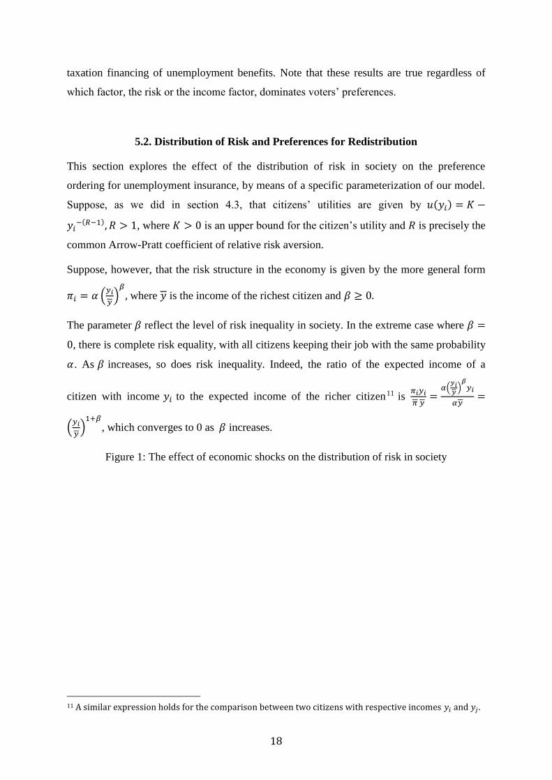
Suppose, however, that the risk structure in the economy is given by the more general form
𝜋𝑖 = 𝛼 (𝑦𝑖
𝑦)𝛽
, where 𝑦 is the income of the richest citizen and 𝛽 ≥ 0.
The parameter 𝛽 reflect the level of risk inequality in society. In the extreme case where 𝛽 =
0, there is complete risk equality, with all citizens keeping their job with the same probability
𝛼. As 𝛽 increases, so does risk inequality. Indeed, the ratio of the expected income of a
citizen with income 𝑦𝑖 to the expected income of the richer citizen11 is 𝜋𝑖𝑦𝑖
𝜋 𝑦=
𝛼(𝑦𝑖𝑦)𝛽𝑦𝑖
𝛼𝑦=
(𝑦𝑖
𝑦)1+𝛽
, which converges to 0 as 𝛽 increases.
Figure 1: The effect of economic shocks on the distribution of risk in society
11 A similar expression holds for the comparison between two citizens with respective incomes 𝑦𝑖 and 𝑦𝑗 .

19
Figure 1 illustrates the effect of the parameter 𝛽. The X-axis displays ex-ante wages, which
vary from 0 to 𝑦. The Y-axis displays the corresponding expected ex-post wages, which vary
from 0 to 𝛼𝑦 . The case 𝛽 = 1 corresponds to the absence of shock, so that the original
distribution of risk is maintained. For 𝛽 > 1 there is an increase in risk inequality and that
increase is more pronounced the higher 𝛽 is. We interpret that situation as a negative
economic shock. Conversely, for 𝛽 < 1 there is a decrease in risk inequality, which is more
pronounced the smaller 𝛽 is. We interpret that situation as a positive economic shock. The
extreme case where 𝛽 = 0 corresponds to the (theoretic) situation where all agents face the
same probability 𝜋𝑖 = 𝛼.
Consider now the first order condition (5). Given the current parameterization, we can write
its RHS as:
𝑅𝐻𝑆(𝑦𝑖) = ℎ(𝜋𝑖). 𝑓(𝑦𝑖) = (𝑅 − 1)(1 − 𝜏)(−𝑅) 𝛼𝑦𝑖(𝛽−𝑅+1)
(𝑦)𝛽 − 𝛼𝑦𝑖𝛽
Taking derivatives with respect to 𝑦𝑖 yields:
beta=0: Homogeneous risk beta=1: Original risk preserving
beta=2: Inequality increasing beta=4: Higher inequality increasing
beta=1/2: Inequality reducing beta=1/4: Higher inequality reducing
𝑦
𝛼𝑦
0

20
𝑅𝐻𝑆′(𝑦𝑖) = (𝑅 − 1)(1 − 𝜏)(−𝑅) 𝛼𝑦𝑖(−𝑅+𝛽)
[(𝑦)𝛽 − 𝛼𝑦𝑖𝛽]2
[(𝛽 − 𝑅 + 1)[(𝑦)𝛽 − 𝛼𝑦𝑖𝛽] + 𝛼𝛽𝑦𝑖
𝛽]
Therefore,
𝑅𝐻𝑆′(𝑦𝑖) > 0 ⟺ 𝑅 < 𝛽 + 1 + 𝛽𝛼𝑦𝑖
𝛽
(𝑦)𝛽 − 𝛼𝑦𝑖𝛽
Let 𝜇(𝛽) = 1 + 𝛽 [1 +𝛼𝑦𝑖
𝛽
(𝑦)𝛽−𝛼𝑦𝑖𝛽]. Then,
(i) If 𝑅 < 𝜇(𝛽), there is security dominance;
(ii) If 𝑅 > 𝜇(𝛽), there is income dominance.
Note now that, as 𝛽 goes to infinity, so does 𝜇(𝛽). Now recall that the higher 𝛽 is, the more
inequality-increasing is the unemployment risk “technology”. Therefore, the more inequality-
increasing the distribution of risk in society is, the more likely it will display security
dominance.
We are now able to evaluate the role of economic shocks. Suppose society is in a relative
homogeneous risk situation at the outset. This may be due to a long period of economic
growth that reduced overall unemployment risk. In the present model, this corresponds to
small values of 𝛽 . Then, it is likely that society displays income dominance. Suppose,
furthermore, that the country is hit by a negative shock, which corresponds to an increase in
𝛽 to 𝛽′> 𝛽. If 𝛽′ is large enough, then society may turn to security dominance.
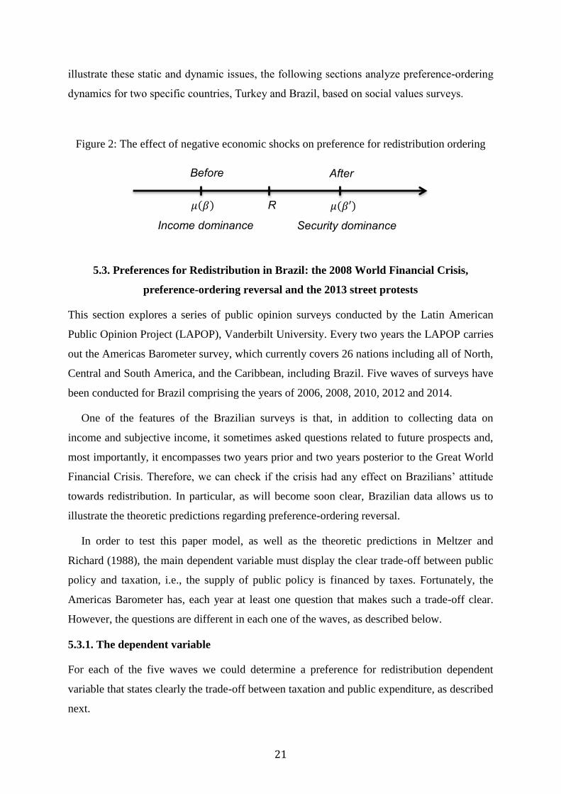
Therefore, a negative shock may generate a preference reversal, in such a way that before the
shock the richer citizens supported higher unemployment insurance whereas after the shock
the biggest supporters for unemployment insurance are the poorer citizens. Figure 2 below
illustrates that situation.
Note that a symmetrical situation may arise in the case of a positive shock. In that case, the
economic recovery may produce a reversal from a situation where the poorer citizens were
the highest supporters of unemployment insurance to a situation where the richer citizens
become the highest supports.
Finally, it may also be the case that the shock is not strong enough to produce any preference
ordering reversal. Therefore, in addition to the preference ordering at a given point in time,
also the dynamic of preference ordering becomes a matter of empirical research. In order to
21
illustrate these static and dynamic issues, the following sections analyze preference-ordering
dynamics for two specific countries, Turkey and Brazil, based on social values surveys.
Figure 2: The effect of negative economic shocks on preference for redistribution ordering
5.3. Preferences for Redistribution in Brazil: the 2008 World Financial Crisis,
preference-ordering reversal and the 2013 street protests
This section explores a series of public opinion surveys conducted by the Latin American
Public Opinion Project (LAPOP), Vanderbilt University. Every two years the LAPOP carries
out the Americas Barometer survey, which currently covers 26 nations including all of North,
Central and South America, and the Caribbean, including Brazil. Five waves of surveys have
been conducted for Brazil comprising the years of 2006, 2008, 2010, 2012 and 2014.
One of the features of the Brazilian surveys is that, in addition to collecting data on
income and subjective income, it sometimes asked questions related to future prospects and,
most importantly, it encompasses two years prior and two years posterior to the Great World
Financial Crisis. Therefore, we can check if the crisis had any effect on Brazilians’ attitude
towards redistribution. In particular, as will become soon clear, Brazilian data allows us to
illustrate the theoretic predictions regarding preference-ordering reversal.
In order to test this paper model, as well as the theoretic predictions in Meltzer and
Richard (1988), the main dependent variable must display the clear trade-off between public
policy and taxation, i.e., the supply of public policy is financed by taxes. Fortunately, the
Americas Barometer has, each year at least one question that makes such a trade-off clear.
However, the questions are different in each one of the waves, as described below.
5.3.1. The dependent variable
For each of the five waves we could determine a preference for redistribution dependent
variable that states clearly the trade-off between taxation and public expenditure, as described
next.
R 𝜇(𝛽)
Before
𝜇(𝛽′)
After
Income dominance Security dominance

22
The 2006 wave has a unique question that makes the tax-public policy trade-off clear. The
question (PR7) is:
“The government should provide less public services, such as health and education, in
order to reduce taxes.”
There were five categorical answers, going from totally disagree to totally agree.
The same question was asked in the 2008 wave (BRAIMP3), but there were just two
categorical answers: agree or disagree.
There were six different question items (VB7) that fit our criterion in the 2010 wave:
“Taking into consideration that taxes would have to increase for the government to be
able to spend more, and that taxes could be reduced if the government spent less or
nothing, for each one of the public services below, how much should the government
spend:
A. Higher education (Public universities and colleges)
B. High school.
C. Elementary and middle school.
D. Public health.
H. Retirement benefits for low-income households, even those who did not
contribute.
K. Retirement benefits for public servants.”
The four categorical answers were:
Increase taxes and spend more
Spend the same amount as presently
Reduce taxes and spend less
Reduce taxes and do not offer this service.
We run Cronbach’s 𝛼 test in order to determine the degree of correlation among those
questions and found a high correlation between the first 5 ones, with 𝛼 = 90.31.
Therefore, we used the mean composite of these 5 questions as our dependent
variable.

23
There were three different questions displaying the tax-expenditure trade-off for the 2012
wave:
“Would you be willing to pay higher taxes than you pay now in order for the
government to spend more money in elementary and middle education? (SOC5)
Would you be willing to pay higher taxes than you pay now in order for the
government to spend more money in public health? (SOC9)
Would you be willing to pay higher taxes than you pay now in order for the
government to spend more money in the Bolsa Familia CCT program?” (SOC11)
There were just two categorical answers: Yes, No.
Once again we calculated Cronbach’s 𝛼 statistic, which lead us to the conclusion
that the first two questions were highly correlated with 𝛼 = 78.01. Therefore, we
used the mean composite of these two first questions as the dependent variable.
Finally, there were exactly one question (TD5) fitting our criterion in the 2014 wave:
“Would you be willing to pay more taxes than you currently so that these taxes
would be used to distribute to the poorer citizens?”
There were 7 categorical answers, from “totally disagree” to “totally agree”.
All the dependent variables were recoded in such a way that higher values mean higher
support for redistribution. For example, for the 2006 dependent variable, the higher
possible choice, 5, means “totally disagree”, whereas for the 2014 dependent variable,
the higher possible choice, 7, means “totally agree”. Furthermore, the observations with
“I don’t know” or no answer were removed from the corresponding sample.
5.3.2. The main explanatory variables
Income, income squared: The income variable classifies respondents according to their
income brackets. The number of income brackets change depending on the wave and
some waves asked the individual respondent’s income (2008, 2010), others their
household income (2012, 2014), while the 2006 asked both. We used the household
income whenever available. In order to allow for the possibility of a nonlinear effect of
income on the preferences for redistribution, we also included the square of the income
variable.
24
Our expectation is that, if there is income dominance, there is a positive correlation
between the income variable the dependent variable, whereas if there is security
dominance, then there is a negative correlation between these variables.
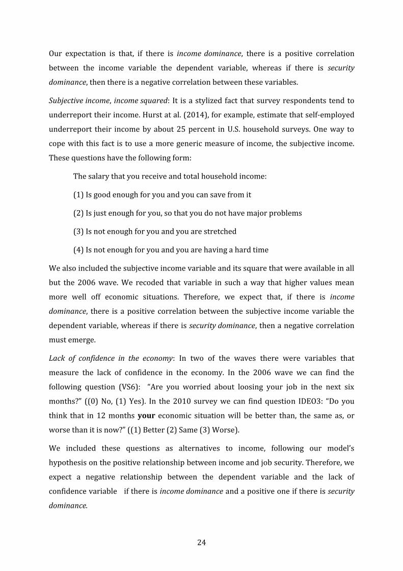
Subjective income, income squared: It is a stylized fact that survey respondents tend to
underreport their income. Hurst at al. (2014), for example, estimate that self-employed
underreport their income by about 25 percent in U.S. household surveys. One way to
cope with this fact is to use a more generic measure of income, the subjective income.
These questions have the following form:
The salary that you receive and total household income:
(1) Is good enough for you and you can save from it
(2) Is just enough for you, so that you do not have major problems
(3) Is not enough for you and you are stretched
(4) Is not enough for you and you are having a hard time
We also included the subjective income variable and its square that were available in all
but the 2006 wave. We recoded that variable in such a way that higher values mean
more well off economic situations. Therefore, we expect that, if there is income
dominance, there is a positive correlation between the subjective income variable the
dependent variable, whereas if there is security dominance, then a negative correlation
must emerge.
Lack of confidence in the economy: In two of the waves there were variables that
measure the lack of confidence in the economy. In the 2006 wave we can find the
following question (VS6): “Are you worried about loosing your job in the next six
months?” ((0) No, (1) Yes). In the 2010 survey we can find question IDEO3: “Do you
think that in 12 months your economic situation will be better than, the same as, or
worse than it is now?” ((1) Better (2) Same (3) Worse).
We included these questions as alternatives to income, following our model’s
hypothesis on the positive relationship between income and job security. Therefore, we
expect a negative relationship between the dependent variable and the lack of
confidence variable if there is income dominance and a positive one if there is security
dominance.
25
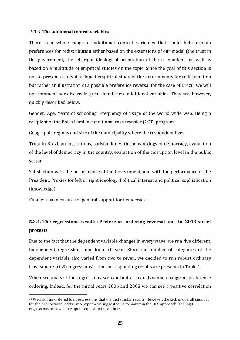
5.3.3. The additional control variables
There is a whole range of additional control variables that could help explain
preferences for redistribution either based on the extensions of our model (the trust in
the government, the left-right ideological orientation of the respondent) as well as
based on a multitude of empirical studies on the topic. Since the goal of this section is
not to present a fully developed empirical study of the determinants for redistribution
but rather an illustration of a possible preference reversal for the case of Brazil, we will
not comment nor discuss in great detail these additional variables. They are, however,
quickly described below.
Gender, Age, Years of schooling, Frequency of usage of the world wide web, Being a
recipient of the Bolsa Familia conditional cash transfer (CCT) program.
Geographic regions and size of the municipality where the respondent lives.
Trust in Brazilian institutions, satisfaction with the workings of democracy, evaluation
of the level of democracy in the country, evaluation of the corruption level in the public
sector.
Satisfaction with the performance of the Government, and with the performance of the
President. Proxies for left or right ideology. Political interest and political sophistication
(knowledge).
Finally: Two measures of general support for democracy.
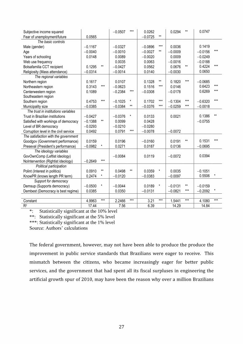
5.3.4. The regressions’ results: Preference-ordering reversal and the 2013 street
protests
Due to the fact that the dependent variable changes in every wave, we run five different,
independent regressions, one for each year. Since the number of categories of the
dependent variable also varied from two to seven, we decided to run robust ordinary
least square (OLS) regressions12. The corresponding results are presents in Table 1.
When we analyze the regressions we can find a clear dynamic change in preference
ordering. Indeed, for the initial years 2006 and 2008 we can see a positive correlation
12 We also run ordered logit regressions that yielded similar results. However, the lack of overall support for the proportional odds ratio hypothesis suggested us to maintain the OLS approach. The logit regressions are available upon request to the authors,

26
between the dependent variable and income (2006) or subjective income (2008), both
significant at the 5% level. This supports the income dominance hypothesis: since Brazil
was in a positive economic growth path, the poorer citizens did not seen to feel the need
for such important provision of public good.
The 2010 picture looks blurry. No income effect is significant and only the fear about
the future variable is significant. Its negative sign suggests that the higher the fear, the
less government the respondent wants, supporting again, but at an indirect level, the
income dominance hypothesis. We shall argue here that Brazilians were confused as to
their support for redistribution in 2010. This confusion is due to the fact that although
the country was severely hit by the international financial crisis in 2009, with null GDP
growth, Lula government created a (artificial) warming of the economy, by reducing
taxes on consumption goods and increasing government expenditure, which lead to a
7.5% growth in 2010. Such a GDP growth level had not happened in the country since
the seventies and led many Brazilians to believe the international crisis had not reached
the country, only to find out, in the following years, its real effects.
After the low growth of 2011, Brazilians became aware of the artificial growth of 2010.
The 2012 and 2014 surveys reflect its effect on the preference for redistribution
ordering. Indeed, the regressions show now an inverse, negative correlation between
the dependent variable and subjective income (2012) or income (2014), compatible
with the security dominance hypothesis. In other words, the poorer a citizen is, the more
government support he favors. This result, significant at 5% for 2012 and at 1% for the
2014 regression, suggests that a preference-ordering reversal has occurred, possibly
because the poor citizens became aware of the severity of the world financial crisis and
its damaging effects to the Brazilian economy, thereby, becoming more supportive of
government programs.
Table 1 – Income, economic confidence, economic shock and preference for redistribution:
Robust OLS regressions for Brazil, 2006 to 2014
Year 2006 2008 2010 2012 2014
The main explanatory variables
Income 0.2126 ** 0. 0421 0.0101 0.0030 0.2425 ***
Income squared 0.0201 0.0022 0.0002 0.0001 0.0131 ***
Subjective income 0.2766 ** 0.0994 0.1525 ** 0.4083
27
Subjective income squared 0.0507 *** 0.0262 0.0294 ** 0.0747
Fear of unemployment/future 0.0565
0.0725 **
The basic controls
Male (gender) 0.1167 0.0327 0.0896 *** 0.0036 0.1419
Age 0.0040 0.0010 0.0027 ** 0.0009 0.0156 ***
Years of schooling 0.0148 0.0089 0.0020 0.0009 0.0249
Web use frequency 0.0035 0.0063 0.0016 0.0188
Bolsafamilia CCT recipient 0.1295 ** 0.0427 0.0562 0.0676 ** 0.4224 ***
Religiosity (Mass attendance) 0.0314 0.0014 0.0140 0.0030 0.0650
The regional variables
Northern region 0.1617 0.0107 0.1328 ** 0.1820 *** 0.0685
Northeastern region 0.3143 *** 0.0623 0.1516 *** 0.0146 0.6423 ***
Centerwestern region 0.1089 0.2384 *** 0.0308 0.0178 0.6269 ***
Southeastern region
Southern region 0.4753 *** 0.1025 * 0.1702 *** 0.1304 *** 0.6320 ***
Municipality size 0.0385 0.0384 ** 0.0376 *** 0.0259 *** 0.0018
The trust in institutions variables
Trust in Brazilian institutions 0.0427
0.0376 * 0.0133 0.0021 0.1386 **
Satisfied with workings of democracy 0.1388 ** 0.0099 0.0428 0.0755
Level of BR democracy 0.0293 0.0210 0.0280
Corruption level in the civil service 0.0492 0.0791 *** 0.0078 0.0072
The satisfaction with the government
Goodgov (Government performance) 0.0159 0.0196 0.0160 0.0191 ** 0.1531 ***
Preseval (President’s performance) 0.0982 * 0.0271 0.0187 0.0136 0.0695
The ideology variables
GovOwnComp (Leftist ideology) 0.0084 0.0119 0.0072 0.0394
NoIntervention (Rightist ideology) 0.2649 ***
Political participation
Polint (Interest in politics) 0.0910 ** 0.0498 ** 0.0359 * 0.0035 0.1051
KnowPR (knows length PR term) 0.2474 * 0.0120 0.0383 0.0097 0.5506 *
Support for democracy
Demsup (Supports democracy) 0.0500 * 0.0044 0.0189 * 0.0131 ** 0.0159
Dembest (Democracy is best regime) 0.0385 0.0350 0.0131 0.0821 *** 0.2092 *
Constant 4.9963 *** 2.2466 *** 3.21 *** 1.5441 *** 4.1080 ***
R2 17.44 7.56 6.39 14.29 14.84
*: Statistically significant at the 10% level
**: Statistically significant at the 5% level
***: Statistically significant at the 1% level
Source: Authors’ calculations
The federal government, however, may not have been able to produce the produce the
improvement in public service standards that Brazilians were eager to receive. This
mismatch between the citizens, who became increasingly eager for better public
services, and the government that had spent all its fiscal surpluses in engineering the
artificial growth spur of 2010, may have been the reason why over a million Brazilians

28
went to the streets during the months of June and July 2013 to demonstrate against the
rise of public transportation cost and the low quality of public services13.
6. The role of trust in the government and political ideology
6.1. The role of trust in the government
In addition to the trade-off between risk and income, one may inquire if the level of trust in
the government could also impact citizens’ support for redistribution.14 In the present study,
the level of confidence in the government is modeled by means of parameter 𝛿, 0 < 𝛿 < 1.
The lower 𝛿 is, the less trusted the government is, whereas the higher that parameter is, the
more trust there is in the government.
In this section we analyze the effect of a change in 𝛿 on the equilibrium redistribution policy
𝜏𝑀. For a comparative static analysis, suppose that neither the distribution of income nor the
risk probabilities change, but that the trust in the government, 𝛿, reduces. This may happen
for different reasons but are typically associated with unexpected events. For example, after
the March 2011 Great Tsunami in Japan, there was a generalized reduction in the trust in the
government due to its handling of the nuclear crises; according to an Associated Press (AP-
GfK) poll held between July and August 2011, 82% of Japanese doubt that the government’s
ability to help them in the event of new disasters.15 Similarly, the corruption scandal in the
biggest Brazilian state company, the Petrobrás, in 2014, greatly reduced citizens’ trust in their
government. According to Brazilian DataFolha institute, the percentage of Brazilians that
considered president Dilma’s government “Bad” or “Very bad” increased from 25% in April
2014 to astounding 60% in one year later, in April 2015, after the corruption scandal.16
Consider again equation (7). The initial effect of a reduction in the parameter 𝛿 is an increase
in the LHS of (7). Therefore, there must also be a variation in the RHS of (7), so that 𝜏𝑀
cannot remain unchanged. Suppose 𝜏𝑀 decreases. Then the LHS of (7) increases further,
whereas its RHS decreases, which configures a contradiction.
13 See Bugarin and Costa e Silva (2014) for details on the 2013 street protests. 14 We are indebted to John Nash, Jr., for stressing this potential factor. 15 See, for example, Telegraph, September 2, 2011. See also Economist, March 10, 2012. The poll press release can be accessed at http://www.ap-gfkpoll.com. 16 DataFolha pool’s press releases are available at http://datafolha.folha.uol.com.br/.
29
Thus, it must be the case that 𝜏𝑀 increases. Therefore, when there is an aggregate shock that
reduces overall trust in government, the median voter favors more redistribution. This may
strike as an unexpected result. Indeed, the less society trusts the government, the more
redistribution it favors. However, one can understand that result noticing that low trust in
government means that society expects less public output with the same amount of taxation.
Therefore, one way to compensate for the reduced public output is to increase taxation.
Suppose the shock is related to evidence of corruption. Then, if corruption suddenly increases
in a country, which could happen, for example, if a more corrupt party takes office, then the
popular pressure towards higher redistributions increases, which potentially brings about an
additional source of instability in a possibly already unstable political environment perturbed
by corruption.
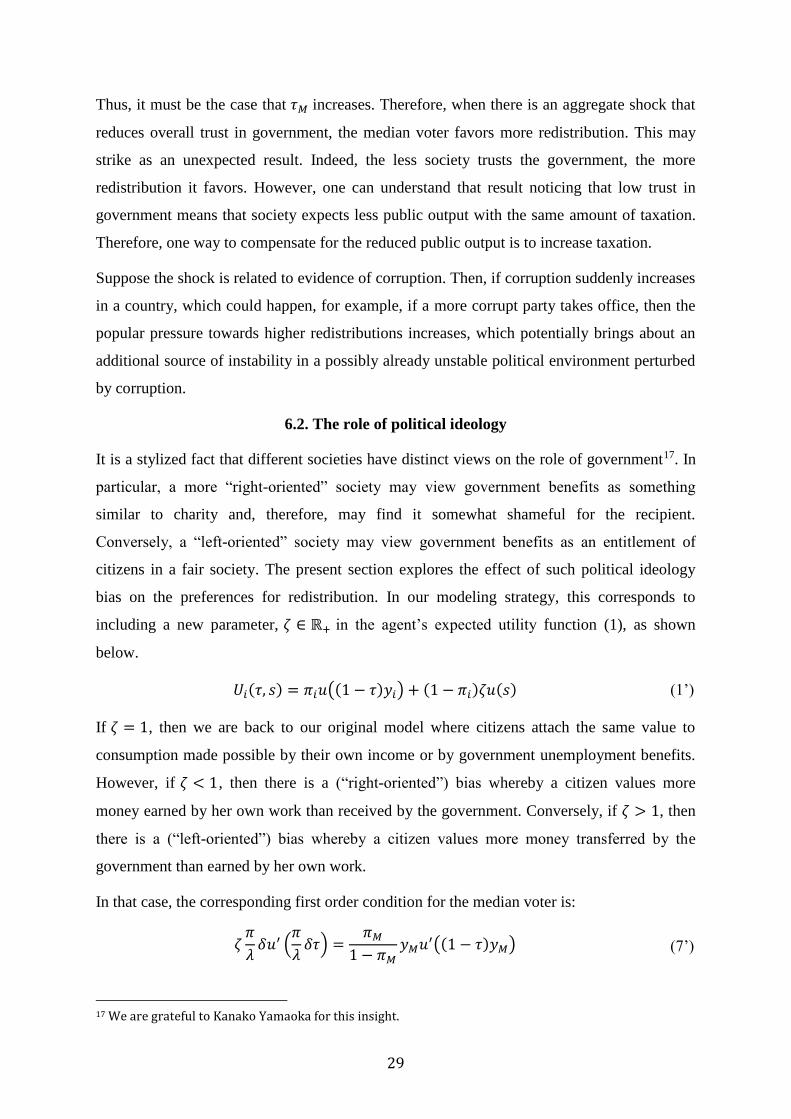
6.2. The role of political ideology
It is a stylized fact that different societies have distinct views on the role of government17. In
particular, a more “right-oriented” society may view government benefits as something
similar to charity and, therefore, may find it somewhat shameful for the recipient.
Conversely, a “left-oriented” society may view government benefits as an entitlement of
citizens in a fair society. The present section explores the effect of such political ideology
bias on the preferences for redistribution. In our modeling strategy, this corresponds to
including a new parameter, 휁 ∈ ℝ+ in the agent’s expected utility function (1), as shown
below.
𝑈𝑖(𝜏, 𝑠) = 𝜋𝑖𝑢((1 − 𝜏)𝑦𝑖) + (1 − 𝜋𝑖)휁𝑢(𝑠) (1’)
If 휁 = 1, then we are back to our original model where citizens attach the same value to
consumption made possible by their own income or by government unemployment benefits.
However, if 휁 < 1, then there is a (“right-oriented”) bias whereby a citizen values more
money earned by her own work than received by the government. Conversely, if 휁 > 1, then
there is a (“left-oriented”) bias whereby a citizen values more money transferred by the
government than earned by her own work.
In that case, the corresponding first order condition for the median voter is:
휁𝜋
𝜆𝛿𝑢′ (
𝜋
𝜆𝛿𝜏) =
𝜋𝑀
1 − 𝜋𝑀𝑦𝑀𝑢′((1 − 𝜏)𝑦𝑀) (7’)
17 We are grateful to Kanako Yamaoka for this insight.

30
Then, the effect of political ideology is to multiply by 휁 the left hand side of equation (7).
Consider now a right-oriented society: 휁 < 1. Then, the LHS of (7) decreases. Therefore, 𝜏
must change. If 𝜏 were to increase, the LHS would decrease further whereas the RHS would
increase, a contradiction. Hence, 𝜏 must decrease. In other words, the median voter in a
politically right-oriented society prefers less government intervention in the economy.
Conversely, it is trivial to show that in a left-oriented society in which 휁 > 1, the median
voter prefers higher levels of public policy provision.
The result we find here is compatible with Hibbs (1977) theory of a partisan bias in the public
policy, according to which left-wing parties prefer bigger governments whereas right-wing
ones prefer smaller government. Furthermore, it explains why a country such as the USA
supports less social policies than Europe, where social-welfare state ideology is more
established. In other words, our model helps explain the USA-Europe debate presented in
section 4.5, without having to appeal to the POUM hypothesis.
7. Conclusion
The present article tries to understand on a theoretic point of view the delicate relationship
between wealth, economic confidence, economic shocks and preferences for redistribution. A
first theoretic result shows that this relationship is not straightforward and depends basically
on two aspects of individual’s preferences. If individuals care most strongly about job
security, then the poorer they are and the less confident in the economy they are, the more
government they favor. On the other hand, if individuals care most strongly about income,
then the poorer they are and the less economic confidence they have, the less government
they want. These findings, which we call the “security-income trade-off” extends the
preliminary results presented in Bugarin & Hazawa (2014) and is a new result in the
literature. It shows that the one-way result in Meltzer and Richard (1981) may not always be
true, as the work of Moene and Wallerstein also show. But differently from Moene and
Wallerstein (2001, 2003), we show that a switch in preference ordering may happen within
the same type of social policy: unemployment insurance. As a consequence, we challenge
their interpretation based on the target population of the policy and conclude that whether
citizens favor more or less government, as their income change, has more to do with risk
aversion and changes in the distribution of unemployment risk in society, i.e., the confidence
in the economy. In particular, we show that the same society may display a switch in citizens’

31
preference ordering due to unexpected external shocks. We illustrate our theoretic predictions
analyzing the case of Brazil before and after the 2008 international financial crisis and find
evidence that there was an preference-ordering reversal in Brazil due to the crisis, in such a
way that before the crisis there was income dominance, i.e., the poorer a citizen is the less
government he favors, whereas after the crisis citizens’ preferences came to display security
dominance, i.e., the poorer a citizen is, the more government she favors. In particular, the
preference-ordering reversal may help explain the unprecedented mass protests that took over
a million Brazilians to the streets during the month of July 2013.
Furthermore, the present article also analyzed what happens when there is an aggregate shock
that affects overall confidence in the economy. In that case, regardless of the tradeoff job
security-income, the effect of an aggregate reduction in economic confidence in the economy
is a higher focus on social policy. Therefore, society unambiguously favors bigger
government if it suffers an aggregate shock that reduces overall economic confidence.
Conversely, the effect of an aggregate increase in economic confidence in the economy is a
lower support for social policy. Therefore, society unambiguously favors smaller
governments if it receives an aggregate shock that increases overall economic confidence.
In addition, our model helps explain how political ideology affects social preferences for
redistribution in such a way that more right-oriented societies prefer smaller governments
whereas more left-oriented ones prefer bigger governments.
References
Alesina, A. F. and P. Giuliano, (2009) “Preferences for Redistribution” NBER working paper
number 14825.
Barro, R., (1973). “The control of politicians: An economic model” Public Choice, 14(1):19-
42.
Benabou, R. and E. Ok, (2001) “Social Mobility and the Demand for Redistribution: the
POUM Hypothesis” Quarterly Journal of Economics, 116: 447-487.
Bugarin, M. and J. R. da Costa e Silva (2014) “From the Diretas Já to the Passe Livre street
demonstrations: 30 years of citizen-led institutional consolidation in Brazil” Iberoamericana,
36(1): 9-26.

32
Bugarin, M. and Y. Hazama (2014) “Consumer economic confidence and preference for
redistribution: Main equilibrium results” Economics Bulletin, 34(3): 2002-2009.
Bugarin, M. and L. Vieira (2008) “Benefit sharing: An incentive mechanism for social
control of government expenditure” The Quarterly Review of Economics and Finance, 48:
673-690.
Choi, E.K. and C. F. Menezes (1985) “On the Magnitude of Relative Risk Aversion”
Economics Letters 18: 125-128.
Diebold, F. X., D. Neumark and D. Polsky (1994) “Job Stability in the United States” NBER
working paper number 4859.
Farber, H. S. (2011) “Job Loss in the Great Recession: Historical Perspective from the
Displaced Workers Survey, 1984-2010” Working paper number 564 Industrial Relations
Section, Princeton University.
Friend, I. and M. E. Blume (1975) “The Demand for Risky Assets”. American Economic
Review 65(5): 900-922.
Hurst, E., Li, G. and B. Pugsley (2014) “Are Household Surveys Like Tax Forms? Evidence
from Income Underreporting of the Self-Employed”. Review of Economics and Statistics,
96(1): 19-33.
Hibbs, D.A. (1977) “Political Parties and Macroeconomic Policy”. American Political
Science Review 71: 1467-1487.
Lindert, P. (2004) Growing Public - Social Spending and Economic Growth since the
Eighteenth Century, Cambridge University Press: Cambridge, MA.
Meltzer, A. H., and S. F. Richard (1981) “A Rational Theory of the Size of Government”
Journal of Political Economy 89(5): 914-27.
Moene, K. O. and E. Barth (2012) “The Equality Multiplier” Working paper.
http://www.sv.uio.no/esop/english/research/publications/working-papers/Imult_revised.pdf.
Moene, K. & M. Wallerstein (2003) “Earnings inequality and welfare spending – A
disaggregated analysis” World Politics 55: 485-516.
Moene, K. & M. Wallerstein (2001) “Inequality, Social Insurance, and Redistribution”
American Political Science Review, 95(4): 859-874.
33
Piketty, T. (1995) “Social Mobility and Redistributive Politics” Quarterly Journal of
Economics CX: 551–583.
Persson, T. and G. Tabellini (2000) Political Economics – Explaining Economic Policy, MIT
Press: Cambridge, MA.
Rehm, P. (2011) “Social Policy by Popular Demand” World Politics 63(2): 271-299.
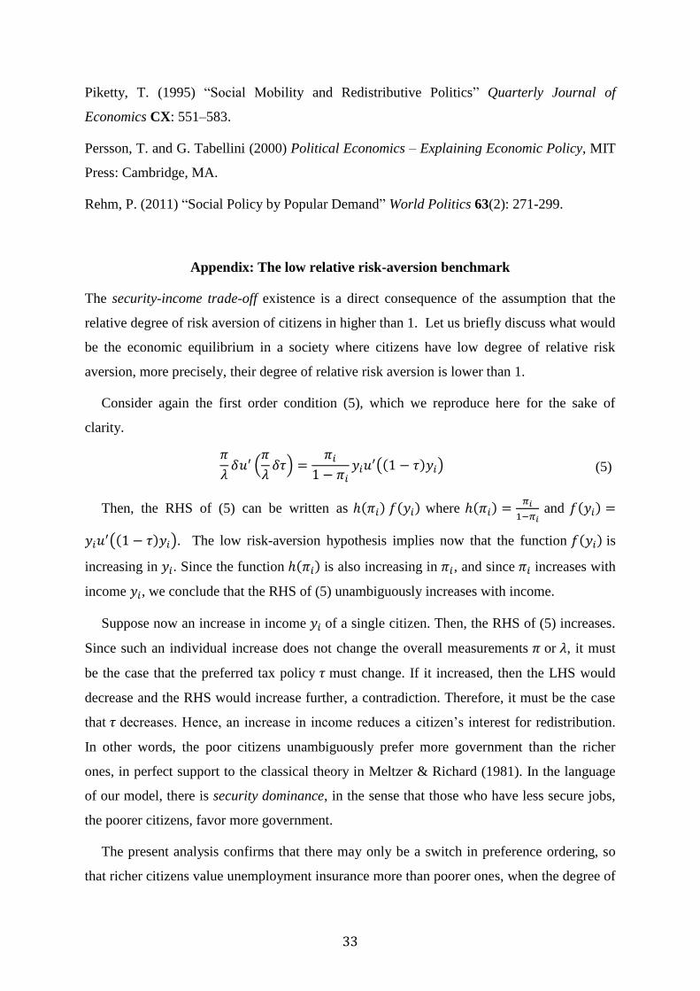
Appendix: The low relative risk-aversion benchmark
The security-income trade-off existence is a direct consequence of the assumption that the
relative degree of risk aversion of citizens in higher than 1. Let us briefly discuss what would
be the economic equilibrium in a society where citizens have low degree of relative risk
aversion, more precisely, their degree of relative risk aversion is lower than 1.
Consider again the first order condition (5), which we reproduce here for the sake of
clarity.
𝜋
𝜆𝛿𝑢′ (
𝜋
𝜆𝛿𝜏) =
𝜋𝑖
1 − 𝜋𝑖𝑦𝑖𝑢
′((1 − 𝜏)𝑦𝑖) (5)
Then, the RHS of (5) can be written as ℎ(𝜋𝑖) 𝑓(𝑦𝑖) where ℎ(𝜋𝑖) =𝜋𝑖
1−𝜋𝑖 and 𝑓(𝑦𝑖) =
𝑦𝑖𝑢′((1 − 𝜏)𝑦𝑖). The low risk-aversion hypothesis implies now that the function 𝑓(𝑦𝑖) is
increasing in 𝑦𝑖. Since the function ℎ(𝜋𝑖) is also increasing in 𝜋𝑖, and since 𝜋𝑖 increases with
income 𝑦𝑖, we conclude that the RHS of (5) unambiguously increases with income.
Suppose now an increase in income 𝑦𝑖 of a single citizen. Then, the RHS of (5) increases.
Since such an individual increase does not change the overall measurements 𝜋 or 𝜆, it must
be the case that the preferred tax policy 𝜏 must change. If it increased, then the LHS would
decrease and the RHS would increase further, a contradiction. Therefore, it must be the case
that 𝜏 decreases. Hence, an increase in income reduces a citizen’s interest for redistribution.
In other words, the poor citizens unambiguously prefer more government than the richer
ones, in perfect support to the classical theory in Meltzer & Richard (1981). In the language
of our model, there is security dominance, in the sense that those who have less secure jobs,
the poorer citizens, favor more government.
The present analysis confirms that there may only be a switch in preference ordering, so
that richer citizens value unemployment insurance more than poorer ones, when the degree of
34
(absolute) risk aversion is high enough (higher than 1). In particular, low risk-averse societies
will always push elected politicians in the direction of bigger governments as the median
voter income decreases, in accordance with Meltzer and Richard (1981)’s framework.