Embed Size (px)
Citation preview


“We are all faced throughout our lives with agonizing decisions, moralchoices. Some are on a grand scale. Most of these choices are on lesserpoints.But we define ourselves by the choices we have made.We are in fact the sum total of our choices.Events unfold so unpredictably, so unfairly, human happiness doesnot seem to have been included in the design of creation. It is onlywe with our capacity to love that give meaning to the indifferentuniverse.And yet most human beings seem to have the ability to keep tryingand even to find joy from simple things like their family, their work,and from the hope that future generations might understand more.”-Dr. LevyWoody Allen’s “Crimes and Misdemeanors”, 1989


ACKNOWLEDGEMENTS
I would like to thank Professor Erasmo Viola who gave me the chance ofcontinuing studying after graduating and of attending the Ph.D. program inStructural Mechanics at the University of Bologna.I am deeply indebted to Professor Ferdinando Auricchio and I sincerely thankhim for the support and scientific tuition he has been giving to me. I wouldlike to thank him for he has taught me the meaning of excellence in research.I would like to thank Professor Franco Brezzi, Professor Donatella Marini andProfessor Carlo Lovadina for their unique kindness in accepting me within theacademic environment of the Institute of Applied Mathematics and Informa-tion Technology and of the Department of Mathematics in Pavia.I would like to thank Professor Fiorella Sgallari for the unvaluable support shehas provided to let me visit and work in Pavia.I also would like to thank Professor Phillip L. Gould of the Civil EngineeringDepartment of the Washington University in St. Louis for the many usefulscientific discussions and for being such a good friend to me since I was asimple undergraduate student.A deep feeling of gratitude goes to my friend Lourenco Beirao da Veiga whohas worked shoulder-to-shoulder with me since I first came to Pavia in January2004.
Pavia, March 13th, 2006


Sommario
Il tema di ricerca su cui verte questa tesi e connesso alla modellazione costi-tutiva di materiali a comportamento inelastico non lineare. Il filone che si escelto di approfondire riguarda lo studio, lo sviluppo e l’implementazione dinuovi algoritmi di integrazione per problemi algebrico-differenziali non lineari,inerenti la modellazione costitutiva di materiali elastoplastici tipo von-Misescon incrudimento.
La teoria della plasticita e, come noto, un argomento classico della Mecca-nica dei continui e si caratterizza per essere una disciplina che attrae l’interessesia di ingegneri che di matematici. Tale caratteristica e sostanzialmente dovutaa ragioni di carattere storico e, nella fattispecie, allo sviluppo della teoria delleequazioni differenziali a derivate parziali e della teoria delle disequazioni vari-azionali riscontrato nella seconda meta del secolo scorso. Tale sviluppo hainfatti permesso una piu profonda comprensione dei caratteri fisici fondamen-tali dei fenomeni elastoplastici ed ha messo a disposizione strumenti idoneialla analisi dei modelli costitutivi e delle formulazioni variazionali dei problemimeccanici di interesse ingegneristico.
E nota la elevata complessita ed il carattere prettamente nonlineare deimodelli matematici in discorso. Un filone di ricerca ormai di rilievo in questosettore e quindi quello dello sviluppo di robusti schemi di integrazione di talimodelli, in grado di fornire un’accurata approssimazione numerica del com-portamento del materiale. Detti metodi risultano infatti essenziali nell’ imple-mentazione di codici di calcolo (ad esempio codici commerciali agli elementifiniti) per la risoluzione approssimata di problemi a valori iniziali e dati albordo per materiali a comportamento elastoplastico.
Questo lavoro si colloca all’interno di questo ultimo settore di ricerca ede strutturato in modo da fornire una introduzione al problema elastoplasticoquanto piu completa possibile. Il primo capitolo propone alcuni richiami es-senziali di Meccanica dei solidi deformabili e di teoria dell’elasticita. Il sec-ondo capitolo riguarda la cosiddetta teoria classica o teoria matematica dellaplasticita e si concentra sulla formulazione della legge costitutiva per materialia comportamento elastoplastico di tipo von-Mises con incrudimento lineare enon lineare.
Il terzo capitolo propone la formulazione variazionale del problema a valoriiniziali e dati al bordo dell’equilibrio di un continuo tridimensionale costituitoda materiale elastoplastico. In tale capitolo sono forniti alcuni risultati dibuona posizione del problema. Il quarto capitolo introduce alla risoluzionenumerica del problema variazionale, utilizzando il metodo degli elementi finitiper la discretizzazione spaziale e schemi basati su metodi alle differenze finite
ii
per la discretizzazione temporale.Il capitolo quinto costituisce la parte innovativa della tesi ed e incentrato
sulla famiglia di metodi d’integrazione cosiddetta a base esponenziale. La tec-nica alla base di questi metodi prevede la riscrittura del modello costitutivo divon-Mises a partire dalla sua formulazione classica, mediante l’adozione di unopportuno fattore integrante scalare, che governa l’evoluzione temporale delflusso plastico. Il sistema dinamico governante, cosı riformulato, ammette unaforma evolutiva caratteristica di tipo quasi-lineare e, sotto opportune ipotesi,puo essere integrato nel tempo e risolto al passo, utilizzando la tecnica dellemappe esponenziali. I vantaggi offerti dalla nuova classe di metodi esponen-ziali sono evidenziati dall’analisi delle proprieta numeriche e dal confronto coni classici metodi alle differenze finite su esempi numerici. Il capitolo sestopresenta una serie di test numerici che hanno lo scopo di valutare la preci-sione e l’accuratezza dei nuovi algoritmi e quindi validarne l’applicabilita nellasimulazione di problemi di interesse ingegneristico.
Completano la tesi due brevi appendici inerenti elementi introduttivi diAnalisi funzionale e di teoria delle disequazioni variazionali. I contenuti delleappendici possono risultare utili nello studio della teoria matematica dellaplasticita affrontato nei Capitoli 2,3 e 4.
Abstract
The research theme upon which this thesis is based regards the constitutivemodeling of nonlinear inelastic materials. The main topic is concerned withthe analysis, the development and the implementation of a new class of inte-gration algorithms for differential-algebraic nonlinear problems arising in theconstitutive modeling of von-Mises elastoplastic hardening materials.
The theory of plasticity, as it is well known, is a classical part of continuumMechanics and is characterized by being a discipline which attracts both thescientific interest of engineer scientists and mathematicians. This fact is mainlydue to historical reasons and, in particular, to the development of the theoryof partial differential equations and of the theory of variational inequalitiestaken place in the second half of the last century. This development has infact made it possible a deeper comprehension of the fundamental physicalmeanings of elastoplastic phenomena and has provided useful theoretical toolsfor the analysis of the constitutive models and of the variational formulationof the mechanical problems of interest.
Given the high complexity and the preeminent nonlinear nature of suchmathematical models, another relevant research challenge in this area is thedevelopment of rubust numerical methods for the integration of such models.

iii
The numerical schemes in argument need to be as precise as possible in orderto accurately reproduce the constitutive response of real elastoplastic materialsin computational enviroments (such as commercial finite element codes).
This work is set within this last research field and is structured in such away that the introduction of the elastoplastic constitutive problem remains ascomplete as possible, in order to carry out both the engineering and the math-ematical aspects of the problem. The first chapter proposes some fundamentalconcepts of Mechanics of deformable material bodies and of theory of elastic-ity. The second chapter is centred on the so-called classical or mathematicaltheory of plasticity. This chapter focuses in particular on the formulationof the von-Mises constitutive law for elastoplastic materials with linear andnonlinear hardening.
The third chapter proposes the analysis of the variational formulation of theinitial boundary value problem of equilibrium for three-dimensional continuumbodies constituted of elastoplastic material. In this chapter also some theo-retical results on the well-posedness of the variational problem are exposed.The fourth chapter introduces to the numerical solution of the variational pro-blem of elastoplastic equilibrium, within the context of a finite element spacediscretization and of classical finite difference time discretization schemes.
Chapter 5 constitutes the innovative part and, being the core of the thesis,focuses on the new class of exponential-based integration schemes for von-Mises elastoplastic models. The basic technique underneath the applicationof these schemes prescribes the rewriting of the original constitutive modelusing a suitable integration factor which governs the evolution of plastic flow.The ensuing differential-algebraic dynamical system results in a characteristicquasi-linear evolutive equation which, under proper hypotheses, may be inte-grated and solved stepwise, using exponential maps. The advantages grantedby the new family of methods are made evident by the theoretical analysis oftheir numerical properties and by the comparison on numerical tests with theclassical finite difference schemes. Chapter 6 presents an extensive series ofnumerical tests which aim to evaluate the precision and the order of accuracyof the new exponential-based algorithms and hence to validate them as feasibletools in practical simulation of problems of engineering interest.
The thesis is completed by two brief appendices concerning mathematicalelements of functional analysis and of theory of variational inequalities. Thecontents of these last two sections may be of some value in the study of themathematical theory of plasticity carried out in chapters 2, 3 and 4.

iv

Contents
1 Continuum Mechanics and Elasticity 31.1 Introduction . . . . . . . . . . . . . . . . . . . . . . . . . . . . . 41.2 Preliminaries and notation . . . . . . . . . . . . . . . . . . . . . 41.3 Kinematics . . . . . . . . . . . . . . . . . . . . . . . . . . . . . 131.4 Equilibrium . . . . . . . . . . . . . . . . . . . . . . . . . . . . . 22
1.4.1 Static equilibrium . . . . . . . . . . . . . . . . . . . . . 221.4.2 Dynamic equilibrium . . . . . . . . . . . . . . . . . . . . 27
1.5 Constitutive relation . . . . . . . . . . . . . . . . . . . . . . . . 291.6 Thermodynamic setting for elasticity . . . . . . . . . . . . . . . 341.7 Initial boundary value problem of equilibrium in linear elasticity 381.8 Thermodynamics with internal variables . . . . . . . . . . . . . 39
2 Elastoplasticity 432.1 Introduction . . . . . . . . . . . . . . . . . . . . . . . . . . . . . 442.2 A one-dimensional elastoplastic model . . . . . . . . . . . . . . 452.3 Three-dimensional elastoplastic behavior . . . . . . . . . . . . . 56
2.3.1 Thermodynamic foundations of elastoplasticity . . . . . 562.3.2 von-Mises yield criterion . . . . . . . . . . . . . . . . . . 702.3.3 General von-Mises plasticity model . . . . . . . . . . . . 76
2.4 Initial boundary value problem of equilibrium in J2 elastoplas-ticity . . . . . . . . . . . . . . . . . . . . . . . . . . . . . . . . . 80
2.5 Elastoplasticity in a convex-analytic setting . . . . . . . . . . . 822.5.1 Results from convex analysis . . . . . . . . . . . . . . . 822.5.2 Basic flow relations of elastoplasticity . . . . . . . . . . 90
3 Variational Formulation of the Elastoplastic Equilibrium Pro-blem 973.1 Introduction . . . . . . . . . . . . . . . . . . . . . . . . . . . . . 983.2 The primal variational formulation . . . . . . . . . . . . . . . . 993.3 The dual variational formulation . . . . . . . . . . . . . . . . . 109
v

vi CONTENTS
4 Discrete Variational Formulation of the Elastoplastic Equili-brium Problem 1134.1 Introduction . . . . . . . . . . . . . . . . . . . . . . . . . . . . . 114
4.1.1 Basics of the finite element method . . . . . . . . . . . . 1154.2 Fully discrete approximation of the dual problem . . . . . . . . 1194.3 Time integration schemes for the dual problem based on finite
difference methods . . . . . . . . . . . . . . . . . . . . . . . . . 1214.4 Solution algorithms for the time integration schemes . . . . . . 125
4.4.1 Elastic predictor . . . . . . . . . . . . . . . . . . . . . . 1274.4.2 Tangent predictor . . . . . . . . . . . . . . . . . . . . . 1294.4.3 Finite element solution of the IBVP of elastoplastic equi-
librium . . . . . . . . . . . . . . . . . . . . . . . . . . . 136
5 Time-integration schemes for J2 plasticity 1475.1 Introduction . . . . . . . . . . . . . . . . . . . . . . . . . . . . . 1485.2 LP plasticity model . . . . . . . . . . . . . . . . . . . . . . . . . 1495.3 Backward Euler’s integration scheme for the LP model . . . . . 150
5.3.1 Integration scheme . . . . . . . . . . . . . . . . . . . . . 1515.3.2 Solution algorithm . . . . . . . . . . . . . . . . . . . . . 1525.3.3 BE scheme elastoplastic consistent tangent operator . . 153
5.4 Generalized midpoint integration scheme for the LP model . . 1545.4.1 Integration scheme . . . . . . . . . . . . . . . . . . . . . 1545.4.2 Solution algorithm . . . . . . . . . . . . . . . . . . . . . 1555.4.3 MPT scheme elastoplastic consistent tangent operator . 157
5.5 ENN exponential-based integration scheme for the LP model . 1585.5.1 A new model formulation . . . . . . . . . . . . . . . . . 1585.5.2 Integration scheme . . . . . . . . . . . . . . . . . . . . . 1625.5.3 Solution algorithm . . . . . . . . . . . . . . . . . . . . . 1645.5.4 ENN scheme elastoplastic consistent tangent operator . 166
5.6 ENC exponential-based integration scheme for the LP model . 1695.6.1 ENC scheme: an enforced consistency variant of the
ENN scheme . . . . . . . . . . . . . . . . . . . . . . . . 1695.7 ESC-ESC2 exponential-based integration schemes for the LP
model . . . . . . . . . . . . . . . . . . . . . . . . . . . . . . . . 1705.7.1 An innovative model formulation . . . . . . . . . . . . . 1705.7.2 Integration scheme . . . . . . . . . . . . . . . . . . . . . 1735.7.3 Solution algorithm . . . . . . . . . . . . . . . . . . . . . 1765.7.4 ESC2 scheme elastoplastic consistent tangent operator . 178
5.8 Theoretical analysis of algorithmical properties of the ESC andESC2 schemes . . . . . . . . . . . . . . . . . . . . . . . . . . . . 181

CONTENTS vii
5.8.1 Yield consistency . . . . . . . . . . . . . . . . . . . . . . 1825.8.2 Exactness whenever Hiso = 0 . . . . . . . . . . . . . . . 1825.8.3 Exactness under proportional loading . . . . . . . . . . 1825.8.4 Accuracy . . . . . . . . . . . . . . . . . . . . . . . . . . 1865.8.5 Convergence . . . . . . . . . . . . . . . . . . . . . . . . 1905.8.6 Two lemmas . . . . . . . . . . . . . . . . . . . . . . . . 196
5.9 NLK plasticity model . . . . . . . . . . . . . . . . . . . . . . . 2045.10 Backward Euler’s integration scheme for the NLK model . . . . 205
5.10.1 Integration scheme . . . . . . . . . . . . . . . . . . . . . 2065.10.2 Solution algorithm . . . . . . . . . . . . . . . . . . . . . 2065.10.3 BEnl scheme elastoplastic consistent tangent operator . 210
5.11 Generalized midpoint integration scheme for the NLK model . 2105.11.1 Integration scheme . . . . . . . . . . . . . . . . . . . . . 2115.11.2 Solution algorithm . . . . . . . . . . . . . . . . . . . . . 2125.11.3 MPTnl scheme elastoplastic consistent tangent operator 215
5.12 ESC2nl exponential-based integration scheme for the NLK model2165.12.1 A model reformulation . . . . . . . . . . . . . . . . . . . 2165.12.2 Integration scheme . . . . . . . . . . . . . . . . . . . . . 2215.12.3 Solution algorithm . . . . . . . . . . . . . . . . . . . . . 2255.12.4 ESC2nl scheme elastoplastic consistent tangent operator 2275.12.5 Brief review of the numerical properties of the ESC2nl
method . . . . . . . . . . . . . . . . . . . . . . . . . . . 232
6 Numerical tests 2356.1 Introduction . . . . . . . . . . . . . . . . . . . . . . . . . . . . . 2366.2 Numerical tests setup . . . . . . . . . . . . . . . . . . . . . . . 236
6.2.1 Mixed stress-strain loading histories . . . . . . . . . . . 2376.2.2 Iso-error maps . . . . . . . . . . . . . . . . . . . . . . . 2396.2.3 Initial boundary value problems . . . . . . . . . . . . . 2416.2.4 Material parameters . . . . . . . . . . . . . . . . . . . . 243
6.3 Numerical tests on the LP model . . . . . . . . . . . . . . . . . 2456.3.1 Mixed stress-strain loading histories . . . . . . . . . . . 2456.3.2 Iso-error maps . . . . . . . . . . . . . . . . . . . . . . . 2556.3.3 Initial boundary value problems . . . . . . . . . . . . . 256
6.4 Numerical tests on the NLK model . . . . . . . . . . . . . . . . 2626.4.1 Mixed stress-strain loading histories . . . . . . . . . . . 2626.4.2 Iso-error maps . . . . . . . . . . . . . . . . . . . . . . . 2636.4.3 Initial boundary value problems . . . . . . . . . . . . . 272

viii CONTENTS
A Results from Functional Analysis 279A.1 Generalities . . . . . . . . . . . . . . . . . . . . . . . . . . . . . 279A.2 Function spaces . . . . . . . . . . . . . . . . . . . . . . . . . . . 289
A.2.1 The spaces Cm(Ω), Cm(Ω) and Lp(Ω) . . . . . . . . . . 289A.2.2 Sobolev spaces . . . . . . . . . . . . . . . . . . . . . . . 294A.2.3 Spaces of vector-valued functions . . . . . . . . . . . . . 301
B Elements of Theory of Variational Inequalities 305B.1 Variational formulation of elliptic boundary value problems . . 305B.2 Elliptic variational inequalities . . . . . . . . . . . . . . . . . . 315B.3 Parabolic variational inequalities . . . . . . . . . . . . . . . . . 316


2 CONTENTS

Chapter 1
Continuum Mechanics andElasticity
Introduzione
Questo capitolo e dedicato ai concetti fondamentali della Meccanica dei solidideformabili e della elasticita lineare. Segue un breve sommario dei contenutidel capitolo.
La Sezione 1.2 richiama gli elementi di algebra vettoriale e tensoriale chevengono utilizzati nella tesi. La Sezione 1.3 riguarda la Cinematica del corpomateriale. In detta sezione si definiscono le fondamentali misure di defor-mazione e viene messo in evidenza il caso delle deformazioni infinitesime. LaSezione 1.4 riguarda la formulazione dell’equilibrio per un corpo materiale.Vengono qui presentati gli assiomi dell’equilibrio statico e dell’equilibrio di-namico, le leggi di bilancio del momento lineare ed angolare, la forma localedell’equazione di equilibrio. La Sezione 1.5 costituisce una breve presentazionedella legge costitutiva per materiali a comportamento elastico lineare isotropocon un accenno alle proprieta fondamentali del tensore dei moduli elastici.
La Sezione 1.6 e incentrata sulla prima e sulla seconda legge della Ter-modinamica e tratta, in particolare, il caso di solidi costituiti da materialeelastico lineare isotropo soggetti a trasformazioni isoterme. La Sezione 1.7presenta la formulazione locale negli spostamenti per il problema a valori in-iziali e dati al bordo dell’equilibrio, per solidi deformabili di materiale elasticolineare isotropo. Da ultimo, la Sezione 1.8 introduce i concetti utilizzati nelcapitolo seguente riguardante la teoria classica della plasticita. In tale sezionesi presenta una trattazione termodinamica generale, adatta allo studio di ma-teriali a comportamento inelastico non lineare. In particolare viene introdottala cosiddetta teoria termodinamica a variabili interne. Per ovvie ragioni, la
3
4 1. CONTINUUM MECHANICS AND ELASTICITY
trattazione di questa sezione si limita al caso della elasticita lineare.Gli elementi di Meccanica del continuo ed elasticita richiamati nel pre-
sente capitolo sono tratti preminentemente da [14, 20], mentre gli argomentidi Termodinamica seguono principalmente la trattazione in [41].
1.1 Introduction
This chapter is devoted to fundamental concepts of Mechanics of deformablesolids and of linear elasticity. In what follows we give a brief outline of thecontents of the chapter.
In Section 1.2 we recall the elements of vector and tensor algebra that areused throughout the thesis. Section 1.3 is concerned with the kinematics of adeformable material body. In this section the fundamental strain measures aredefined and special emphasis is given to the small deformation case. Section1.4 regards the formulation of equilibrium for a material body. Here we presentthe axioms of static and dynamic equilibrium, the balance laws of linear andangular momentum and the local form of the equilibrium equation. Section 1.5is a concise review of the constitutive law for linear elastic isotropic materials.In this section we briefly examine the basic properties of the elastic tensor andthe form of the linear elastic constitutive law.
Section 1.6 focuses on the first and second laws of Thermodynamics andparticularly on the special case of linear elastic bodies undergoing isothermaltransformations. Section 1.7 presents the classical displacement local formu-lation of the equilibrium boundary value problem for a deformable body con-stituted of linear elastic material. Finally, Section 1.8 sets the stage for thelater developments on the elastoplastic theory developed in Chapter 2. In fact,in this section, we give a general framework which is particularly suitable forstudying nonlinear inelastic materials. For obvious reasons the treatment ismomentarily dedicated to linear elasticity. In particular the so-called thermo-dynamic theory with interval variables is addressed. In this chapter the ele-ments of continuum Mechanics and elasticity are basically taken from [14, 20],while the Thermodynamics arguments are presented following [41].
1.2 Preliminaries and notation
Vectors and tensors
In this work, we deal with different types of mathematical objects, namelywith scalars, second-order tensors and fourth-order tensors as well as with

1.2. PRELIMINARIES AND NOTATION 5
generalized vector and matrix operators. Scalars are indicated by italic letterslike
a, α, A
Vectors, second-order tensors and generalized vector operators are denoted byboldface letters like
a, α, A, Σ
while fourth-order tensors and generalized matrix operators are indicated withuppercase boldblackboard letters like
A, G
The summation convention for repeated indices, or Einstein convention, willbe used in our developments1
We refer to a three dimensional Euclidean space R3 and thus make use ofa Cartesian coordinate system equipped with an orthonormal basis (e1, e2, e3)chosen once and for all. Components of vectors and tensors are systematicallyreferred to such a basis. The vector a of the space R3 is identified by theordered set aiT , 1 ≤ i ≤ 3, which defines its coordinates with respect to theabove canonical basis and where i is the free index varying between 1 and 3,such that
a = aiei
In the following we adopt the following notations for vectors of R3:
• Compacta
• Indicialai = a|i
• Engineeringa = a1, a2, a3T
The scalar product of two vectors a and b is denoted by a · b and is definedby:
a · b = aibi1The summation convention requires that a repeated index in a multiplicative term implies
the presence of a summation over the possible index range. Consistently, a non-repeatedindex in a multiplicative term implies that it may assume indifferently any value in thepossible index range.

6 1. CONTINUUM MECHANICS AND ELASTICITY
The Euclidean norm of a vector a is defined according to:
‖ a ‖= (a · a)1/2
The Euclidean space R3 with the natural operations introduced above formsa vector space, indicated in the following as lin.
The cross product or vector product c of two vectors a and b is a vectorc = a × b, orthogonal to both a and b, with length equal to the area of theparallelogram defined by the vectors a and b and direction defined accordingto the right-hand rule. We then have the following expression in terms ofcomponents
c = a× b = (aiei)× (ajej) = aibj(ei × ej) = aibjEijkek
where, for 1 ≤ i, j, k ≤ 3, Eijk is the permutation symbol, i.e. Eijk = +1 for(i, j, k) a cyclic permutation, Eijk = −1 for (i, j, k) an anticyclic permutationand Eijk = 0 otherwise. The cross product returns a vector which is orthogonalto the plane containing the two original vectors. Second-order tensor areobjects defined to generalized such a property in the sense that they operateon a vector returning a vector.
A second-order tensor τ is defined as a linear operator mapping vectors intovectors. Clearly, dealing with a three-dimensional space, to completely definethe action of a second-order tensor, it is necessary to consider at least the actionon three independent vectors of lin, such as the three basis vectors. Sincethe action of the second-order tensor on the three basis vectors is to returnthree new vectors, we may conclude that second-order tensors are in generalidentified through a set of nine scalar components. The space of second-ordertensors with the natural operation defined in the following form a vector space,indicated in the sequel as Lin
The fundamental operation to construct the space of second-order tensoris the tensor product of two vectors a and b, indicated as a ⊗ b and definedas
(a⊗ b)c = (b · c)a ∀a,b, c ∈ lin
The tensor products ei⊗ej of the basis vectors of lin are a set of second-ordertensors, providing a suitable basis for expressing the components of a second-order tensor of the space Lin. In particular we define the ijth component of atensor τ as
τij = ei · τej
1.2. PRELIMINARIES AND NOTATION 7
which implies that the second-order tensor τ can be expressed in componentform as
τ = τij(ei ⊗ ej)
In this work we adopt the following notations for a second-order tensor of thespace Lin:
• Compactτ
• Indicialτij = τ |ij
• Engineering
[τ ] =
τ11 τ12 τ13τ21 τ22 τ23τ31 τ32 τ33
The transpose of a second-order tensor τ is indicated in compact notation byτT and defined by the following relation
τ T |ij = τji
The trace of a second-order tensor τ is a scalar-valued function defined as
tr(τ ) = τii
We use the symbol Linsym to indicate the subspace of Lin of symmetric second-order tensors, i.e.
Linsym = τ ∈ Lin : τ = τT (1.1)
We use the symbol Linsym0 to indicate the subspace of Lin of symmetric second-
order traceless tensors, i.e.
Linsym0 = τ ∈ Linsym : tr(τ ) = 0 (1.2)
The action of a second-order tensor τ onto a vector a is a vector b ∈ lin
b = τa
defined according to
bi = (τa) · ei = [(τlmel ⊗ em)(akek)] · ei = τlmak[(el ⊗ em)ek] · ei
= τlmak[el(em · ek)] · ei = τlmak(el · ei)δmk = τlkakδli = τikak
8 1. CONTINUUM MECHANICS AND ELASTICITY
The scalar product or double-dot product of two second-order tensors σ andτ
σ : τ
is a scalar defined by
σ : τ = σijτij
It is noted that
σ : τ = tr(τ T σ)
The multiplication or combination of two second-order tensors σ and τ is asecond-order tensor η
η = στ
defined in the following manner
ηij = σikτkj
The Euclidean norm of a second-order tensor τ induced by the above scalarproduct is
‖ τ ‖= (τ : τ )1/2
The second-order identity tensor I is defined by the relation Ia = a,∀a ∈ lin.The components of the identity tensor are the Kronecker delta, that is
δij =
1 if j = i
0 otherwise
A unique additive decomposition of any second-order tensor τ is given bythe sum of its deviatoric part τdev and its volumetric or spherical part τ vol,respectively defined as
τ vol =13
tr(τ )I τ dev = τ −13
tr(τ ) (1.3)
This definition implies
τ = τ vol + τ vol (1.4)
A fourth-order tensor is defined as a linear operator mapping the space ofsecond-order tensors Lin onto itself. To properly define the action of a fourth-order tensor, it is necessary to consider the action on a second-order tensor

1.2. PRELIMINARIES AND NOTATION 9
basis; since the action of a fourth-order tensor on a second-order tensor is toreturn a second-order tensor, we may conclude that fourth-order tensors arein general defined by a set of eighty-one scalar components. The space offourth-order tensors with the natural operations introduced in the followingform a vector space, indicated in the sequel by Lin.
The fundamental operation to construct the space of fourth-order tensoris the dyadic product of two second-order tensors τ and σ, indicated as τ ⊗σand defined as to return a fourth-order tensor:
D = (τ ⊗ σ) (1.5)
with D ∈ Lin and such that
Dη = (τ ⊗ σ)η = (σ : η)τ = tr(ηT σ)τ ∀η ∈ Lin (1.6)
The tensor products between the second-order basis tensor provide a suitablebasis for expressing the components of a fourth-order tensor of the space Lin.In particular we define the ijklth component of a tensor D as
Dijkl = (ei ⊗ ej) : D(ek ⊗ el)
such that the fourth-order tensor D can be expressed in component form as
D = Dijkl(ei ⊗ ej)⊗ (ek ⊗ el)
In the following we will adopt the following notations for fourth-order tensorof the space Lin:
• CompactD
• IndicialDijkl = D|ijkl
The action of a fourth-order tensor D on a second-order tensor τ is denotedby
σ = Dτ (1.7)
with the following indicial representation
σij = [Dτ ] : (ei ⊗ ej) = [(Dabcd ea ⊗ eb ⊗ ec ⊗ ed) (τkl ek ⊗ el)] : (ei ⊗ ej)= [(Dabkl τkl) ea ⊗ eb] : (ei ⊗ ej) = Dabkl τkl
(1.8)

10 1. CONTINUUM MECHANICS AND ELASTICITY
Besides the dyadic tensor product between second-order tensors, the so-calledsquare tensor products can be also introduced as:
E = A B
F = A B
defined, according to Del Piero [29], such that:
(A B)C = ACBT
(A B)C = ACTBT∀C ∈ Lin
or, equivalently,
(A B)|ijkl = AikBjl
(A B)|ijkl = AilBjk
∀A,B ∈ Lin
The fourth-order identity tensor I, is defined to satisfy the relation Iτ = τ , forany second-order tensor τ . The fourth-order identity tensor, in componentsform, can be shown to be given by
I = ei ⊗ ei ⊗ ei ⊗ ei
or, equivalently
I = δikδjlei ⊗ ej ⊗ ek ⊗ el
Therefore we have
Iijkl = δikδjl
The fourth-order symmetrized identity tensor II , is defined to satisfy the rela-
tion IIτ = 1
2(τ +τ T ), for any second-order tensor τ . Accordingly, II is defined
as:
II =
12
[I I + I I
]or, in indicial notation as:
IIijkl =
12
[IikIjl + IilIjk]
Therefore we have
IIA = 1
2(A + AT ) ∀A ∈ Lin

1.2. PRELIMINARIES AND NOTATION 11
A splitting into volumetric and deviatoric parts of the fourth-order identitytensor of the form
I = Ivol + Idev (1.9)
is achievable by setting
Ivol =13
(I⊗ I)
Idev = I−13
(I ⊗ I)
(1.10)
With the above positions, the volumetric and deviatoric part τ vol and τdev ofany second-order tensor τ are respectively given by:
τ vol = Ivolτ =13
tr(τ ) I =13
(τ : I) I
τ vol = Idevτ = σ − τ vol
(1.11)
Other than vectors and second-order tensor defined over the Euclidean spaceR3, in some selected cases we make use of algebraic vectors or m-tuples. Forinstance, the m-component algebraic vector ξ can be equivalently indicated incompact notation or in algebraic notation as ξ = (ξk) = (ξ1, ..., ξk, ...ξm). It isnoted that the components ξk (1 ≤ k ≤ m) of such a vector may be objects ofdifferent type, namely scalars, vectors or tensors. The use of algebraic vectorswill be specified whenever needed in order to avoid confusion. Similarly, insome cases, use will be made of algebraic or matrix operators. Such matrixoperators will be in general represented in engineering notation as
[G] =[
G11 G12
G21 G22
]It is noted that the components Gij of a matrix operator may be objects ofdifferent type, namely scalars, second-order tensors or fourth-order tensors.The use of matrix operators will be specified whenever needed in order toavoid confusion.
Invariants of second-order tensors
The algebraic problem of finding every scalar λ and every nonzero vector qsuch that
τq = λq

12 1. CONTINUUM MECHANICS AND ELASTICITY
leads to the standard eigenvalue problem. This consists of solving the charac-teristic equation
det(λI− τ ) = 0
This equation can be written equivalently as
λ3 − I1λ2 + I2λ− I3 = 0
where I1(τ ), I2(τ ) and I3(τ ) are the principal scalar invariants of τ . Theprincipal scalar invariants are respectively defined by
I1 = tr(τ ) = λ1 + λ2 + λ3
I2 =12[tr(τ )2 − tr
(τ 2)]
=12(τiiτjj − τijτji) = λ1λ2 + λ2λ3 + λ3λ1
I3 = det τ = λ1λ2λ3
where the scalars λ1, λ2 and λ3 are the eigenvalues of τ as well as the rootsof the characteristic equation (a multiple root is counted repeatedly accordingto its multiplicity). The eigenvalues of a matrix τ are often referred to as theprincipal components of τ .
The gradient of a scalar field φ(x) defined on lin is denoted by ∇φ and itis the vector defined by
∇φ =∂φ
∂xiei
The divergence divu and the gradient ∇u of a vector field u(x) defined on linare respectively a scalar and a second-order tensor field defined by
divu =∂ui
∂xi
∇u =∂ui
∂xjei ⊗ ej
The divergence of a second-order tensor τ defined on lin is a vector defined by
divτ =∂τij
∂xjei

1.3. KINEMATICS 13
For a scalar-valued function f(τ ) defined on Lin, the derivative with respectto τ is defined as a second-order tensor of the following form
∂f(τ )∂τ
=∂f(τ )∂τij
ei ⊗ ej
For a time-dependent quantity z, we will denote with z its partial derivativewith respect to time t.
1.3 Kinematics
Material body
We consider a body B that at the macroscopic level may be regarded ascomposed of material that is continuously distributed in space. Assume thatat any time instant t the body B can be identified with a closed subset, Ω, ofthe tridimensional real space R3:
B ≡ Ω ⊂ R3 (1.12)
Accordingly, it is possible to associate any material point X ∈ B with a pointX ∈ Ω ⊂ R3:
X ∈ B→ X ∈ Ω ⊂ R3 (1.13)
The above identification procedure allows to treat the material body as acontinuum, that is, as a mathematical entity which inherents the continuumpower property of the R3 space [38]. In particular, we may define functionsof position and time over the configuration, perform real analysis, differen-tial calculus operations on such functions and so on. It is also possible toconstruct a mathematical model corresponding to experimental observations,that is, perform experimental observations and assign the measured averagedproperties to a point of the body.
In the present context we start by addressing the kinematics of the bodywhich is the common starting point to describe the behavior of general con-tinuous media. As it is well known, this framework remains independent ofwhat acts on the body and of the constitution of the body itself.
Change of configuration
Let us consider two distinct time instants t0 and t, such that t0 < t. We refer t0as the initial time instant, while we refer t as the current time instant. At timet0 the material body B can be identified with a subset Ω0 ∈ R3, indicated

14 1. CONTINUUM MECHANICS AND ELASTICITY
u X
x X
0
X
Figure 1.1: Current and reference configurations of a material body
as initial or reference configuration, such that at the same time instant thegeneric material point X ∈ B can be identified with a corresponding pointX ∈ Ω0. At time t, the material body B can be identified with a subsetΩ ∈ R3, indicated as current configuration, such that at the same time instantthe generic material point X ∈ B can be identified with a corresponding pointx ∈ Ω. In the above specifications we have set the convention of indicating thereference position vector, X, with an upper case boldface letter and the currentposition vector, x, with a lower case boldface letter. More generally, eitherusing a compact or an indicial notation, quantities relative to the referenceconfiguration are indicated with upper case letters and quantities relative tothe current configuration are indicated with lower case letters.
In view of the identification represented by relation (1.13), it is possibleto construct a map between the reference and the current configuration, indi-cated, in general, as change of configuration or deformation map ϕ. Adoptingin the following both a compact and an indicial notation, we can express thedeformation map ϕ as follows:
x = ϕ(X)xi = ϕi(XJ )
(1.14)
or more precisely as:
ϕ : X ∈ Ω0 ⊂ R3 → x ∈ Ω ⊂ R3
Observing Equation (1.14) it is noted that the conventions on the use of upperand lower case letters to denote respectively reference and current configura-

1.3. KINEMATICS 15
tions quantities is applied also to the subscript relative to the components ofthe reference position vector (indicated with an upper case index (J)) and tothe components of the current position vector ( indicated with a lower caseindex (i)).
The analytical requirement on the deformation map is that it has to respectthe body continuity. This condition can be split in external requirements andinternal requirements, i.e. in requirements relative to the body boundary andto the body interior. In particular, if the body configuration is assigned ona portion of the boundary, indicated as ∂Ωϕ
0 (for example, x = X on ∂Ωϕ0 ,
∀t ≥ t0), then the map should respect such an assignment on such a boundaryportion. Moreover, in the body interior the map should respect the bodycontinuity; from a mathematical point of view this is expressed through thefollowing conditions:
• the map ϕ is a function
• the map ϕ is continuous
• the map ϕ is differentiable with continuous derivatives (class C2)
• the map ϕ is invertible
The gradient of the deformation map, or deformation gradient, F, is definedas:
F = ∇Xϕ
FiJ =∂ϕi
∂XJ
(1.15)
and, without distinguishing between the deformation map, ϕ, and the currentposition, x, (i.e. x ≡ ϕ) the deformation gradient can be also written as:
F = ∇Xx =∂x∂X
FiJ =∂xi
∂XJ
(1.16)
It can be shown that ϕ maps an infinitesimal vector dX, with origin in X,into a vector, dx, with origin in x, as follows:
dx = FdX
dxi = FiJdXJ(1.17)
Accordingly, the deformation gradient is a two-point second-order tensor; infact, it is a second-order tensor since it maps vectors into vectors, but it is

16 1. CONTINUUM MECHANICS AND ELASTICITY
two-point since one component is relative to the reference configuration andone component is relative to the current configuration. This is consistent withthe fact that F operates on vectors defined in the reference configuration andit returns vectors defined in the current configuration. In fact, the indices ofF are still indicated with a lower case letter and with an upper case letterrespectively.
The deformation gradient F = F(X) is in general function of position,since the deformation map is in general non uniform. Likewise, ϕ is in generala nonlinear map in space and F results as its pointwise linearization.
Strain
It is possible to prove that the deformation gradient F = F(X), being apointwise-defined second-order tensor, characterizes the strain status of thepoint X neighborhood. In particular, given F it is possible two compute therelative change in length of a generic fiber emanating from X, as well as thechange in angle between two fibers emanating from X.
The above statement can be derived with the following reasoning. Consideran infinitesimal vector dS, with origin in X and expressed as dS = NdS with Nunit vector (i.e. ‖N‖ = 1). Let us indicate with ds the vector with origin in x,obtained from dS through the deformation map ϕ, that is: ds = FdS = FNdS.Defining the stretch of the vector dS as the elongation of the vector throughthe deformation map, that is, as the ratio between the norm of the vector afterand before the mapping:
λ =‖ds‖‖dS‖ (1.18)
and recalling that ‖N‖ = 1, it holds:
λ2 =ds · dsdS · dS =
(FNdS) · (FNdS)(NdS) · (NdS)
=(FN) · (FN)
N ·N = CN ·N = λ2(N)
(1.19)where C is the right Cauchy-Green deformation tensor, defined as:
C = FTF
CIJ = FaIFaJ
(1.20)
Accordingly:λ = λ(N) = ‖FN‖ =
√CN ·N (1.21)
that is, given F and hence C, we can compute the elongation of any fiber withorigin in X and extremum in a sufficiently small neighborhood of X. Such
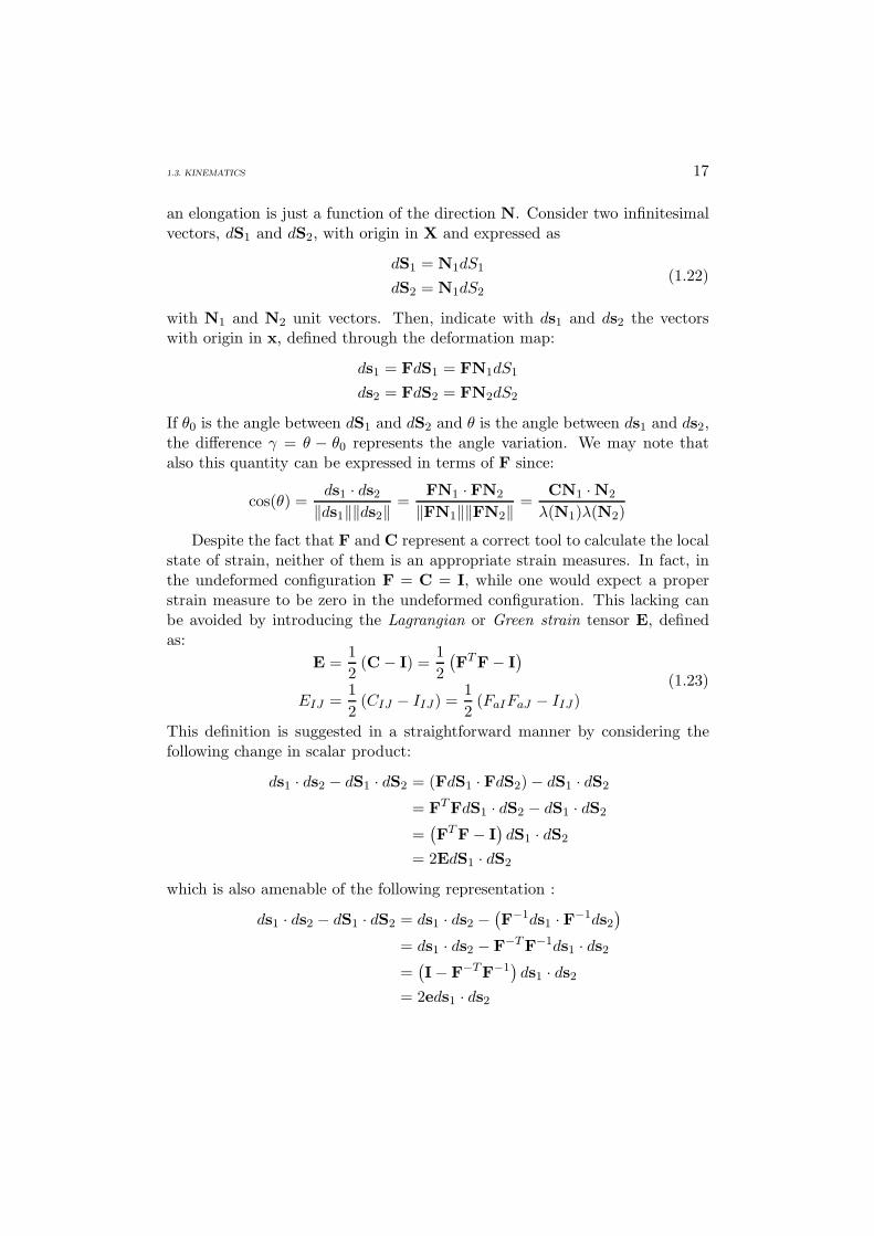
1.3. KINEMATICS 17
an elongation is just a function of the direction N. Consider two infinitesimalvectors, dS1 and dS2, with origin in X and expressed as
dS1 = N1dS1
dS2 = N1dS2(1.22)
with N1 and N2 unit vectors. Then, indicate with ds1 and ds2 the vectorswith origin in x, defined through the deformation map:
ds1 = FdS1 = FN1dS1
ds2 = FdS2 = FN2dS2
If θ0 is the angle between dS1 and dS2 and θ is the angle between ds1 and ds2,the difference γ = θ − θ0 represents the angle variation. We may note thatalso this quantity can be expressed in terms of F since:
cos(θ) =ds1 · ds2
‖ds1‖‖ds2‖=
FN1 ·FN2
‖FN1‖‖FN2‖=
CN1 ·N2
λ(N1)λ(N2)
Despite the fact that F and C represent a correct tool to calculate the localstate of strain, neither of them is an appropriate strain measures. In fact, inthe undeformed configuration F = C = I, while one would expect a properstrain measure to be zero in the undeformed configuration. This lacking canbe avoided by introducing the Lagrangian or Green strain tensor E, definedas:
E =12
(C− I) =12(FTF− I
)EIJ =
12
(CIJ − IIJ) =12
(FaIFaJ − IIJ)(1.23)
This definition is suggested in a straightforward manner by considering thefollowing change in scalar product:
ds1 · ds2 − dS1 · dS2 = (FdS1 · FdS2)− dS1 · dS2
= FTFdS1 · dS2 − dS1 · dS2
=(FTF− I
)dS1 · dS2
= 2EdS1 · dS2
which is also amenable of the following representation :
ds1 · ds2 − dS1 · dS2 = ds1 · ds2 −(F−1ds1 ·F−1ds2
)= ds1 · ds2 − F−TF−1ds1 · ds2
=(I− F−TF−1
)ds1 · ds2
= 2eds1 · ds2
18 1. CONTINUUM MECHANICS AND ELASTICITY
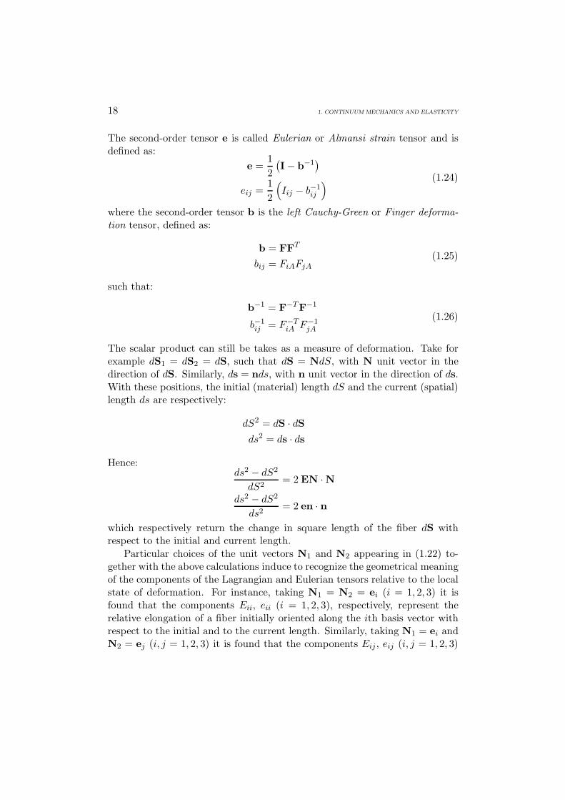
The second-order tensor e is called Eulerian or Almansi strain tensor and isdefined as:
e =12(I− b−1
)eij =
12
(Iij − b−1
ij
) (1.24)
where the second-order tensor b is the left Cauchy-Green or Finger deforma-tion tensor, defined as:
b = FFT
bij = FiAFjA
(1.25)
such that:
b−1 = F−TF−1
b−1ij = F−T
iA F−1jA
(1.26)
The scalar product can still be takes as a measure of deformation. Take forexample dS1 = dS2 = dS, such that dS = NdS, with N unit vector in thedirection of dS. Similarly, ds = nds, with n unit vector in the direction of ds.With these positions, the initial (material) length dS and the current (spatial)length ds are respectively:
dS2 = dS · dSds2 = ds · ds
Hence:ds2 − dS2
dS2= 2 EN ·N
ds2 − dS2
ds2= 2 en · n
which respectively return the change in square length of the fiber dS withrespect to the initial and current length.
Particular choices of the unit vectors N1 and N2 appearing in (1.22) to-gether with the above calculations induce to recognize the geometrical meaningof the components of the Lagrangian and Eulerian tensors relative to the localstate of deformation. For instance, taking N1 = N2 = ei (i = 1, 2, 3) it isfound that the components Eii, eii (i = 1, 2, 3), respectively, represent therelative elongation of a fiber initially oriented along the ith basis vector withrespect to the initial and to the current length. Similarly, taking N1 = ei andN2 = ej (i, j = 1, 2, 3) it is found that the components Eij , eij (i, j = 1, 2, 3)

1.3. KINEMATICS 19
with i = j, respectively, represent the relative change in angle between thefibers initially oriented along the ith and jth reference axis with respect to theinitial and to the current angle between them.
It is convenient to describe the change of configuration introducing thedisplacement field u, defined as the pointwise difference between the currentand the reference vector position:
u(X) = x(X)−X (1.27)
Then the current position vector is given by the sum of the reference positionvector and of the displacement vector:
x = ϕ(X) = X + u(X)
The expression of the deformation map in terms of displacement gives riseto alternative expressions of the strain tensors introduced previously. Forexample, the deformation gradient becomes:
F =∂x∂X
=∂
∂X(X + u) = I +∇Xu (1.28)
which, defining H = ∇Xu, can be written as:
F = I + H (1.29)
Moreover, we may write:
C = FTF = I + H + HT + HTH
E =12
(C− I) =12(H + HT + HTH
) (1.30)
The Eulerian strain tensor (1.30)2 admits the splitting:
E = E1 + E2 = εεε + E2
which identifies the linear and the nonlinear parts of E, respectively as E1 =εεε = (H + HT )/2 and E2 = (HTH)/2.
Small displacement gradient
In many structural engineering problems the deformations can be regarded assmall in some sense. This assumption, which is rigorously formalized, obvi-ously introduces an approximation in the treatment but, nevertheless, permitsto simplify the problem formulation and thus remains of notable interest.

20 1. CONTINUUM MECHANICS AND ELASTICITY
Consider the case of a motion with a small displacement gradient ∇u, thatis:
‖∇Xu‖ = ε with ε 1
Recalling (1.30), the additive decomposition of the strain tensor E in a linearand a nonlinear term, we may prove the following theorem [37].
Theorem 1.3.1 Assume ||∇u|| = ε 1. Then:
2E = C− I +O(ε) = b− I +O(ε) = 2E1 = 2εεε
Furthermore, if F corresponds to a rigid motion, then:
∇u = −∇uT +O(ε)
This proposition asserts that to within an error of order O(ε):
• if the displacement gradient ∇Xu is sufficiently small then the nonlinearterm in (1.30) can be neglected
• the tensors E and εεε coincide as well as the tensors C and b coincide
• the displacement gradient corresponding to a rigid deformation is skew
Under the same assumptions it is also possible to prove that:
det(F)− 1 = div (u) +O(ε) (1.31)
In the following we indicate a deformation map characterized by a small dis-placement gradient field as a small deformation map or simply we talk aboutsmall deformations, that is:
Small deformation ⇔
‖∇Xu‖ 1
εεε = 12
[∇Xu + (∇Xu)T
]Volume change
We are now interested in the evaluation of the unit volume change produced inthe change of configuration of the body by means of the deformation map. Tobegin with it is worth recalling that the volume V of a parallelepiped definedby the vectors a, b and c is given by:
V (a,b, c) = (a× b) · c
Moreover, the following theorem holds:
1.3. KINEMATICS 21
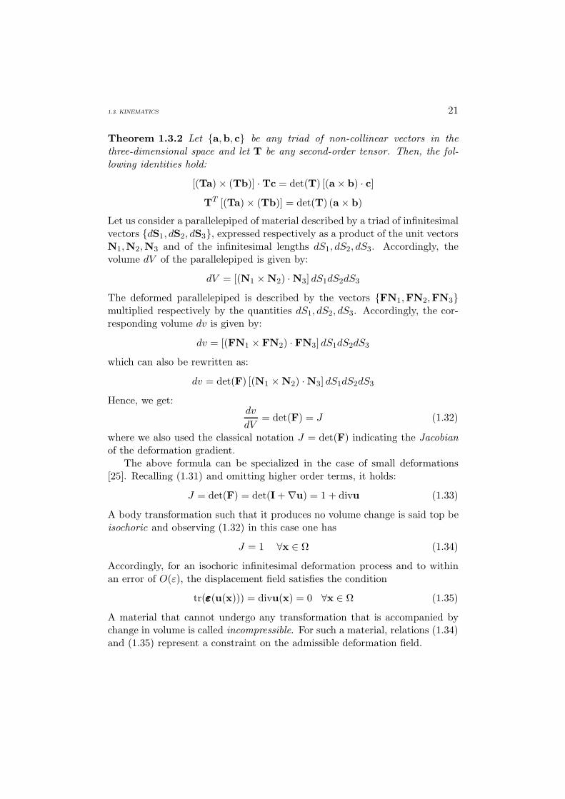
Theorem 1.3.2 Let a,b, c be any triad of non-collinear vectors in thethree-dimensional space and let T be any second-order tensor. Then, the fol-lowing identities hold:
[(Ta)× (Tb)] ·Tc = det(T) [(a× b) · c]
TT [(Ta)× (Tb)] = det(T) (a× b)
Let us consider a parallelepiped of material described by a triad of infinitesimalvectors dS1, dS2, dS3, expressed respectively as a product of the unit vectorsN1,N2,N3 and of the infinitesimal lengths dS1, dS2, dS3. Accordingly, thevolume dV of the parallelepiped is given by:
dV = [(N1 ×N2) ·N3] dS1dS2dS3
The deformed parallelepiped is described by the vectors FN1,FN2,FN3multiplied respectively by the quantities dS1, dS2, dS3. Accordingly, the cor-responding volume dv is given by:
dv = [(FN1 × FN2) · FN3] dS1dS2dS3
which can also be rewritten as:
dv = det(F) [(N1 ×N2) ·N3] dS1dS2dS3
Hence, we get:dv
dV= det(F) = J (1.32)
where we also used the classical notation J = det(F) indicating the Jacobianof the deformation gradient.
The above formula can be specialized in the case of small deformations[25]. Recalling (1.31) and omitting higher order terms, it holds:
J = det(F) = det(I +∇u) = 1 + divu (1.33)
A body transformation such that it produces no volume change is said top beisochoric and observing (1.32) in this case one has
J = 1 ∀x ∈ Ω (1.34)
Accordingly, for an isochoric infinitesimal deformation process and to withinan error of O(ε), the displacement field satisfies the condition
tr(εεε(u(x))) = divu(x) = 0 ∀x ∈ Ω (1.35)
A material that cannot undergo any transformation that is accompanied bychange in volume is called incompressible. For such a material, relations (1.34)and (1.35) represent a constraint on the admissible deformation field.

22 1. CONTINUUM MECHANICS AND ELASTICITY
1.4 Equilibrium
1.4.1 Static equilibrium
This section investigates body static equilibrium conditions, relative either tothe whole body or to body subsets. In particular, the equilibrium is com-prehensive of the relations introducing proper quantities measuring internalforces, i.e. actions exchanged between neighborhood body subsets.
Given a body B in a configuration Ω, we postulate that the interactionbetween the external world and the body can be described through two forcefields:
• a surface force field, or contact force field, t, with dimension of force byunit area and defined on a portion of the current boundary surface, ∂Ωt
2;
• a volume force field, or body force field, b, with dimension of force byunit volume and defined on the current configuration, Ω.
We also postulate that:
• the interaction between any portion of the body Ω′ internal to the body(i.e. such that Ω′ ⊂
Ω) and the remaining part of the body Ω \Ω′ can be
described through a surface force field, indicated also as traction forcefield, with dimension of force by unit area and defined on ∂Ω′. Theseinteraction forces are assumed to be function of the local outward normalto Ω′, and, accordingly, we indicate this field with tn, with the subscriptto express the dependency from the normal n.
Given any portion Ω′ of the body in the current configuration Ω, we can definethe force resultant, r, and the moment resultant, m, relative to Ω′ ⊆ Ω as:
r(Ω′) =∫
Ω′bdv +
∫∂Ω′
tnda
m(Ω′) =∫
Ω′(x× b) dv +
∫∂Ω′
(x× tn) da(1.36)
where x is the current position vector and where the resultant momentum iscomputed with respect to a generic origin o.
Now, defined the force and moment resultants, we may state the
2In general, we set ∂Ωt = ∂Ω \ ∂Ωϕ with ∂Ωϕ the part of the boundary where we assignthe deformation map ϕ; accordingly, we have: ∂Ω = ∂Ωt ∪ ∂Ωϕ .

1.4. EQUILIBRIUM 23
Static Equilibrium Axiom. A deformable body is in equilibrium if andonly if the force resultant and the force momentum on each portion ofthe body are zero, that is, a body B in a configuration Ω is in equilibrium ifand only if:
r(Ω′) = 0 ∀Ω′ ⊆ Ωm(Ω′) = 0 ∀Ω′ ⊆ Ω
(1.37)
or, in a more explicit format, a body B in a configuration Ω is in equilibriumif and only if:∫
Ω′bdv +
∫∂Ω′
tnda = 0 ∀Ω′ ⊆ Ω∫Ω′
(x× b) dv +∫
∂Ω′(x× tn) da = 0 ∀Ω′ ⊆ Ω
(1.38)
Equation (1.38) are also indicated as linear momentum and angular momen-tum balance laws. Moreover, for the case Ω′ ≡ Ω, the above equations spe-cialize as:
r(Ω) =∫
Ωbdv +
∫∂Ωϕ
tnda+∫
∂Ωt
tda = 0
m(Ω) =∫
Ω(x× b) dv +
∫∂Ωϕ
(x× tn) da+∫
∂Ωtn
(x× t) da = 0(1.39)
where we note that the quantity tn in the surface integral on ∂Ωϕ is unknown.We now want to investigate the actions that internal parts of the body
mutually exchange. To do so, let us introduce a surface Σ, ideally dividing thebody Ω in two parts, Ω′
1 and Ω′2, such that Ω′
1∪Ω′2 = Ω, and let us also define:
Γ1 = ∂Ω′1 \Σ and Γ2 = ∂Ω′
2 \ Σ, such that: ∂Ω′1 = Γ1 ∪ Σ and ∂Ω′
2 = Γ2 ∪ Σ.Assuming that the whole body is in equilibrium, by the equilibrium axiom, wehave that each single part of the body should be in equilibrium, hence, alsoΩ′
1 and Ω′2. Without showing all the calculations (refer for instance to [14])
the last statement amounts to the following fundamental result:∫Σ
(tn + t−n) da = 0
which, recalling the arbitrariness of the surface Σ, implies
tn = −t−n (1.40)
The above equation is known as action-reaction principle or as Cauchy recip-rocal principle or as first Cauchy theorem.
24 1. CONTINUUM MECHANICS AND ELASTICITY
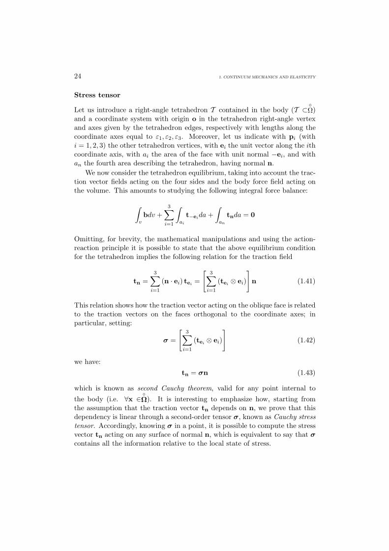
Stress tensor
Let us introduce a right-angle tetrahedron T contained in the body (T ⊂Ω)
and a coordinate system with origin o in the tetrahedron right-angle vertexand axes given by the tetrahedron edges, respectively with lengths along thecoordinate axes equal to ε1, ε2, ε3. Moreover, let us indicate with pi (withi = 1, 2, 3) the other tetrahedron vertices, with ei the unit vector along the ithcoordinate axis, with ai the area of the face with unit normal −ei, and withan the fourth area describing the tetrahedron, having normal n.
We now consider the tetrahedron equilibrium, taking into account the trac-tion vector fields acting on the four sides and the body force field acting onthe volume. This amounts to studying the following integral force balance:
∫vbdv +
3∑i=1
∫ai
t−eida+∫
an
tnda = 0
Omitting, for brevity, the mathematical manipulations and using the action-reaction principle it is possible to state that the above equilibrium conditionfor the tetrahedron implies the following relation for the traction field
tn =3∑
i=1
(n · ei) tei =
[3∑
i=1
(tei ⊗ ei)
]n (1.41)
This relation shows how the traction vector acting on the oblique face is relatedto the traction vectors on the faces orthogonal to the coordinate axes; inparticular, setting:
σ =
[3∑
i=1
(tei ⊗ ei)
](1.42)
we have:
tn = σn (1.43)
which is known as second Cauchy theorem, valid for any point internal tothe body (i.e. ∀x ∈
Ω). It is interesting to emphasize how, starting from
the assumption that the traction vector tn depends on n, we prove that thisdependency is linear through a second-order tensor σ, known as Cauchy stresstensor. Accordingly, knowing σ in a point, it is possible to compute the stressvector tn acting on any surface of normal n, which is equivalent to say that σcontains all the information relative to the local state of stress.

1.4. EQUILIBRIUM 25
From Equation (1.43), it is possible to obtain a physical interpretation forthe components of the stress tensor, noting that:
σij = ei · σej = ei ·[
3∑i=1
(tei ⊗ ei)
]ej = ei · tej (1.44)
Hence, the ijth component of σ is the ith component of the traction vectoracting on the face with normal vector ej. The reader should be warned thatsome authors reverse the convention [3, 38, 53].
It is also interesting to note that Equation (1.42) indicates that σ is fullydetermined once we know the three vectors te1 , te2 , te3 ; accordingly, σ isknown once we know nine independent components, which are exactly thenumber of components in a second-order tensor.
Static equilibrium equations
We now want to transform the equilibrium requirements from the global inte-gral format of Equation (1.38) to a local differential format. To do so, we startrecalling that, given any tensor field G defined on a region Ω′ with normal nand boundary ∂Ω′, the divergence theorem of a tensor field states:∫
∂Ω′Gnda =
∫Ω′
div (G)dv (1.45)
Applying this equality to Equation (1.38)1, we get:∫Ω′
bdv +∫
∂Ω′tnda =
∫Ω′
bdv +∫
∂Ω′σnda =
∫Ω′
(b + div σ) dv = 0
and since this equality must hold for all Ω′ ⊆ Ω, we get the correspondinglocal form of the equilibrium equation:
div σ + b = 0
σij,j + bi = 0(1.46)
where the subscript comma indicates differentiation. Accordingly, this is a setof three linear partial differential equations.
To derive the local form of the angular momentum balance, we start mul-tiplying Equation (1.38)2 with an arbitrary and constant vector field h:∫
Ω′[(x× b) · h] dv +
∫∂Ω′
[(x× tn) · h] da =∫Ω′
[(x× b) · h] dv +∫
∂Ω′[(x× σn) · h] da = 0
(1.47)

26 1. CONTINUUM MECHANICS AND ELASTICITY
Now, recalling the cyclic nature of the triple product, the definition of trans-pose for a second-order tensor and the equality:
div(GTv
)= v · div G + G : ∇v
valid for any tensor field G and any vector field v, we may note that:∫∂Ω′
[(x× σn) · h] da =∫
∂Ω′[(h× x) · σn] da
=∫
∂Ω′
[σT (h× x) · n
]da
=∫
Ω′div
[σT (h× x)
]dv
=∫
Ω′[(h× x) · div σ + σ : ∇ (h× x)] dv
=∫
Ω′[(x× div σ) · h + σ : ∇ (h× x)] dv
Accordingly, Equation (1.47) becomes:∫Ω′
[(x× b) · h] dv +∫
Ω′[(x× div σ) · h + σ : ∇ (h× x)] dv =∫
Ω′[x× (div σ + b) · h + σ : ∇ (h× x)] dv =∫
Ω′[σ : ∇ (h× x)] dv = 0
(1.48)
where we used the balance of linear momentum, i.e. div σ + b = 0. Notingthat ∇x = I, we have:
∇ (h× x) = H
with H a skew-symmetric tensor such that: Hv = h × v for any vector v.Moreover,
σ : H = tr(σTH) = ei · σTHei
hence, Equation (1.48) reduces to:∫Ω′
[h · (ei × σei)] dv = 0
with an implied sum on i. Recalling that h and Ω′ are arbitrary, we finallyget:
ei × σei = 0 (1.49)

1.4. EQUILIBRIUM 27
To understand the real implication of Equation (1.49), we may consider thekth component of the previous equation, expressing also the tensor σ in com-ponents:
ek · [ei × σei] = ek · [ei × (σabea ⊗ eb) ei] = ek · [ei × σabeaIib]= ek · [ei × σaiea] = [σai (ek · ei × ea)] = σaiEkia
The above equaiton can be written in a more explicit format as:
σai = σai (a = i) (1.50)
or in compact notation as:σ = σT (1.51)
Therefore, the balance of angular momentum implies the symmetry of stresstensor σ. In conclusion, the local form of the balance equations are respec-tively:
div σ + b = 0 in Ω
σ = σT in Ω
t = σn on ∂Ωt
(1.52)
or in indicial notation
σij,j + bi = 0 in Ωσij = σji in Ω
ti = σijnj on ∂Ωt
(1.53)
1.4.2 Dynamic equilibrium
Given a motion ϕ of a body B, the linear momentum, l, and the angularmomentum, a, of any body portion Ω′ ⊆ Ω at time t are defined as:
l(Ω′, t) =∫
Ω′ρudv
a(Ω′, t) =∫
Ω′(x× ρu) dv
(1.54)
where the angular momentum is computed with respect to a generic origin oand with the mass density ρ uniform at any point in the body.
Deriving in time it follows that for every portion Ω′:
l(Ω′, t) =∫
Ω′ρudv
a(Ω′, t) =∫
Ω′(x× ρu) dv
(1.55)
28 1. CONTINUUM MECHANICS AND ELASTICITY
Recalling that for any portion Ω′ ⊆ Ω we can define a force resultant, r, anda moment resultant, m, given respectively by:
r(Ω′) =∫
Ω′bdv +
∫∂Ω′
tnda
m(Ω′) =∫
Ω′(x× b) dv +
∫∂Ω′
(x× tn) da(1.56)
it is possible to state the
Dynamic Equilibrium Axiom. A deformable body is in equilibrium if andonly if the force resultant and the force momentum on each portion satisfythe linear and angular momentum balance laws. Accordingly, a body B in aconfiguration Ω is in equilibrium if and only if:
r(Ω′) = l(Ω′) ∀Ω′ ⊆ Ωm(Ω′) = a(Ω′) ∀Ω′ ⊆ Ω
(1.57)
where we neglect to indicate time dependency and where l and a are the rateof the linear and of the angular momentum, as defined in (1.55). Accordingly,(1.57) can be rewritten as:∫
Ω′bdv +
∫∂Ω′
tnda =∫
Ω′ρudv ∀Ω′ ⊆ Ω∫
Ω′(x× b) dv +
∫∂Ω′
(x× tn) da =∫
Ω′(x× ρu) dv ∀Ω′ ⊆ Ω
(1.58)
Dynamic equilibrium equations
Consider first the law of balance of linear momentum (1.58)1. Taking intoconsideration relationship (1.43) and using again the divergence theorem (1.45)one can rewrite the surface integral extended to the boundary ∂Ω′ as∫
∂Ω′tnda =
∫∂Ω′
σnda =∫
Ω′div σdv
so that Equation (1.58)1 becomes∫Ω′
[ρu− b− div σ] dv = 0 (1.59)
Since the portion Ω′ is arbitrary, the integrand in (1.59) must vanish. Thiscondition gives the local form of the equation of motion
div σ + b = ρu (1.60)

1.5. CONSTITUTIVE RELATION 29
For the cases in which all the given data are independent of time, we haveu = u(x), σ = σ(x) and the response of the body will be independent of timeas well and the equation of motion recovers the equation of static equilibrium(1.46). Examining the law of balance for the angular momentum, we mayperform similar manipulations to those that lead to Equation (1.60) and findagain the symmetry of the Cauchy stress tensor:
σT = σ
σij = σji
Remark 1.4.1 All the equilibrium considerations presented so far are relativeto the natural configuration where equilibrium should hold, hence they are allrelative to the current configuration Ω and written in terms of geometricalquantities relative to the current configuration Ω. However, thanks to theinvertibility of the map x = ϕ(X) presented in Equation (1.14) and relatingthe current configuration Ω to the reference configuration Ω0, we can also write:
• equilibrium equations relative to the current configuration Ω in term ofgeometrical quantities relative to the reference configuration Ω0
• equilibrium equations relative to the reference configuration Ω0 in termof geometrical quantities relative to the reference configuration Ω0
In particular, when a small deformation regime is considered, the distinctionbetween reference and current configuration may be ignored. In this case thealternative forms of equilibrium listed above coincide.
1.5 Constitutive relation
Basic relations
We have so far described the equations of motion and the strain-displacementsrelations within the framework of infinitesimal deformation. In componentform these equations are given by a set of nine partial differential equations:three from the balance law and six from the strain-displacement relation (ad-mitting the symmetry of εεε). Correspondingly, we have a total of fifteen un-knowns represented by the six independent components of the strain and ofthe stress and by the three displacement components. It is clear that sixadditional equations are needed in order to have a well defined problem.
From physical considerations we may infer that the missing equationsshould regard the behavior of the material constituting the body. This further

30 1. CONTINUUM MECHANICS AND ELASTICITY
set of equations are the constitutive equations. In the present section we willbe involved in summarizing the basic equations and properties related to linearelastic materials.
A material body is said to be elastic if the stress is entirely determined bythe current state of deformation. Assuming the strain tensor εεε as a measureof the local state of deformation we have
σ = σ(εεε)σij = σij(εab)
(1.61)
This position implies that the stress cannot depend on the deformation historyand, in particular, on the path followed to reach the actual state. However,introducing the density of internal work done in going from an initial strain,εεεi, to a final strain, εεεf , on a path Γεεε as:
W intΓεεε
=∫
Γεεε
σ(εεε) : dεεε
it is in general possible that W intΓεεε
may depend on the specific strain path Γεεε.In the absence of internal constraints and under proper mathematical con-
ditions, Equation (1.61) can be inverted:
εεε = εεε(σ)εij = εij(σab)
(1.62)
It is also interesting to consider an incremental format of relation (1.61), inthe form:
σ = Ctgεεε (1.63)
where the superposed dot indicates a time derivative and Ctg is the tangent
elastic tensor defined as:C
tg =∂σ
∂εεε(1.64)
An elastic material is said to be linear if the stress and the strain are relatedthrough a (linear) relation of the type:
σ = Cεεε
σij = Cijklεkl(1.65)
where the fourth-order tensor C is termed the elastic tensor.Given the symmetry of the second-order tensor εεε, we may write
σij = Cijklεlk = Cijlkεkl

1.5. CONSTITUTIVE RELATION 31
Exploiting the symmetry of the stress tensor σ, we have
σji = Cjilkεlk = Cjiklεklεkl
which implies the following equalities
Cijkl = Cijlk = Cjikl = Cjilk
The above relation states that the elastic tensor which by definition relatessymmetric second-order tensors, possesses the the so-called minor symmetries
Cijkl = Cijlk = Cjikl
and thus presents, at most, 21 independent components.In addition, the elastic tensor C is said to be positive definite if
εεε : Cεεε > 0 ∀εεε ∈ Linsym (1.66)
while it is said to be strongly elliptic [60, 75] if
(a⊗ b) : C (a⊗ b) > 0 ∀a,b ∈ lin (1.67)
Finally, C is said to be pointwise stable [60] if there exists a constant α > 0such that
εεε : Cεεε ≥ α ‖ εεε ‖2 ∀εεε ∈ Linsym (1.68)
Clearly pointwise stability implies, but is not implied, by strong ellipticity.Moreover, pointwise stability is equivalent to pointwise positive definiteness,under the assumption that C is continuous on Ω.
Inverting relationship (1.65), we may obtain the strain as a function ofstress
εεε = Aσ (1.69)
and define the fourth-order compliance tensor A, inverse of C. Equivalently
A (Cεεε) = εεε ∀εεε, εεεT = εεε
and
C (Aσ) = εεε ∀σ, σT = σ

32 1. CONTINUUM MECHANICS AND ELASTICITY
Isotropic elasticity
A material that has no preferred directions in a way that it resists to exter-nal agencies independently of its orientation is said to be isotropic [41]. Theproperty of isotropy for a linear elastic material reduces the twenty-one in-dependent components of the elastic tensor to two and from a mathematicalstandpoint amounts to say that the elastic tensor C presents also the so-calledmajor symmetries
Cijkl = Cklij
In this hypothesis the elastic tensor admits the following representation [57]
C = λ (I⊗ I) + 2µII (1.70)
where the constants λ and µ are called Lame moduli and depend on the ma-terial. This corresponds to a linear elastic relation between stress and strainin the form:
σ = λ(tr(εεε))I + 2µεεε (1.71)
Bearing in mind the previous definition and recalling the volumetric/deviatoricsplitting of the fourth-order identity tensor (cf. (1.10)), we may perform thedecoupling into volumetric and deviatoric parts of the elastic tensor as well.Thus, the following relationship is derived
C =[λ (I⊗ I) + 2µI
I]
= [(3λ+ 2µ)Ivol + 2µIdev]= [3KIvol + 2µIdev]
with 3K = 3λ+ 2µ, such that:
σ = Cεεε = [3KIvol + 2µIdev]εεε= 3KIvolεεε + 2µIdevεεε
Recalling the split of a second-order tensor into its volumetric and deviatoriccomponents (cf. (1.11)), we may write:
σ = pI + s
εεε =13θI + e
where p = (1/3)tr(σ) and θ = tr(εεε) are respectively the pressure and thevolumetric deformation, while s and e are respectively the stress and strain

1.5. CONSTITUTIVE RELATION 33
deviator. The uncoupled volumetric and deviatoric constitutive equations thusread:
p = Kθ
s = 2µe(1.72)
The scalar coefficient µ is referred to as the shear modulus, while the materialcoefficient K = (λ+2/3µ) is called the bulk modulus and represents a measureof the ratio between the spherical stress and the change in volume [57]. Theshear modulus µ is often denoted by G, especially in the engineering literature.With the above specifications, the isotropic linear elastic constitutive equations(1.72) can be rewritten as follows
p = Kθ (1.73)s = 2Ge (1.74)
where s and e are the deviatoric stress and strain, respectively. The quantitiesp = 1/3tr(σ) and θ = tr(εεε) are associated to the volumetric part of thestress and of the strain and are respectively called pressure and volumetricdeformation.
It is worth trying to see if it is possible to find another choice of coeffi-cients that define the linear isotropic elastic behavior of a material. We maytry to find another set of parameters that play the same role as the Lamemoduli coefficients, from studying the mechanical behavior of an isotropic lin-ear elastic rod subjected to uniaxial stress. Suppose that the rod lies alignedwith the x1 axis and that it is subjected to a uniform stress σ11 = 0, beingthe remaining stress components zero. Limiting our investigation to the ra-tios σ11/ε11 and ε33/ε11, or equivalently, ε22/ε11 we may define the followingmaterial parameters
Young’s modulus E =σ11
ε11
Poisson’s ratio ν = −ε22
ε11
which measure, respectively, the slope of the stress-strain curve pertainingto the material which the rod is made of and the lateral contraction of therod. Physical and experimental considerations suggest that the preceding arepositive quantities. In what follows it will be seen how further restrictions,induced by thermodynamic considerations, hold on the quantities E and ν.

34 1. CONTINUUM MECHANICS AND ELASTICITY
Using relation (1.70) and recalling the form of the stress and of the straintensors in pure tension
[σ] =
σ11 0 00 0 00 0 0
[εεε] =
ε11 0 00 ε22 00 0 ε33
it is possible to correlate the pairs λ, µ and E, ν. Omitting the completecalculation, one obtains
E =µ (3λ+ 2µ)
(µ+ λ)(1.75)
µ =λ
2 (µ+ λ)(1.76)
With the above relation, it is possible to invert relationship (1.71) and obtaina useful expression of strain in terms of stress involving E and µ
εεε = E−1 [(1 + ν) σ − νtr (σ) I] (1.77)
The above linear relationship between strain and stress, valid for isotropicmedia, is commonly referred to as Hooke’s law. Applying the definitions ofpointwise stability and of strong ellipticity to the fourth-order elastic tensor(see (1.67) and (1.68)), a set of bounds on the material parameters can bederived for the material parameter Young’s modulus E [60]. These conditionsallow to state that a linear elastic isotropic material is
• pointwise stable if and only if µ > 0 and 3λ+ 2µ > 0 or, equivalently, if
and only if E > 0 and −1 < ν <12
• strongly elliptic if and only if µ > 0 and λ + 2µ > 0 or, equivalently, if
and only if E > 0 and ν <12
or ν > 1
1.6 Thermodynamic setting for elasticity
A common procedure in Mechanics of solids is to introduce a constitutivemodel as a set of relations that hold from a thermodynamic standpoint [4, 57,41]. Precisely, the most favorable context is within a thermodynamic theorywith internal variables. In this section, we present the linear elastic materialbehavior in this fashion. The treatment of the elastoplastic case is carried outin Chapter 2.

1.6. THERMODYNAMIC SETTING FOR ELASTICITY 35
Suppose that a material body is subjected to a body force b in its interiorand to a surface traction t upon its boundary. Analogously, the body willbe acted by thermal equivalents of the previous mechanical sources: a heatsource r per unit volume in the interior and a heat flux q across its boundaryunit area. The first law of Thermodynamics, which essentially is a balance ofenergy statement, indicates that for any part Ω′ of the body Ω, the rate ofchange of total energy plus kinetic energy equals the amount of work done onthat part by the mechanical forces plus the heat supply. Mathematically, thelaw can be formulated in the form
d
dt
∫Ω′
(e+12ρ ‖ u ‖2)dv =
∫Ω′
b · udv +∫
∂Ω′tn · uda+
∫Ω′rdv −
∫∂Ω′
q · nda
(1.78)
where e is the internal energy density, u is the velocity field, while ∂Ω′ rep-resents the boundary of Ω′. The minus sign before the last integral in (1.78)appears, since the heat flux vector q points outward the surface Ω′ as well as n.The preceding formulation can be simplified applying the divergence theoremto the term involving the surface traction which, invoking the symmetry of σ,becomes (cf. (1.52)3)∫
∂Ω′tn · uda =
∫∂Ω′
σn · uda =∫
Ω′σ : ∇udv +
∫Ω′
divσ · udv
=∫
Ω′σ : εεεdv +
∫Ω′
divσ · udv
Substituting the last result in (1.78) and recalling the equation of balance oflinear momentum (1.58), the first law can be rewritten as
d
dt
∫Ω′edv =
∫Ω′
σ : εεεdv +∫
Ω′rdv −
∫∂Ω′
q · nda (1.79)
where it is implicitly assumed that εεε = εεε(u). The local form of the abovebalance law follows from the requirement that all the involved field variablesare sufficiently regular. This hypothesis allows to convert the surface integralon ∂Ω′ appearing in (1.79) using the divergence theorem. Thus we are lead to∫
Ω′(e− σ : εεε− r + divq)dv = 0
which, for the arbitrariness of the portion Ω′, gives
e = σ : εεε + r − divq (1.80)

36 1. CONTINUUM MECHANICS AND ELASTICITY
It is useful to introduce also the notions of entropy η per unit volume orentropy density. This notion is given through the absolute temperature θ > 0.Accordingly, it is assumed that the entropy flux across the bounding surface∂Ω′ into a material body Ω′ is given by∫
∂Ω′θ−1q · nda
while the entropy supplied by the exterior is∫Ω′θ−1rdv
The second law of Thermodynamics states that the rate of increase in entropyin the body is not less than the total entropy supplied to the body by the heatsources. The second law can thus be formalized as an integral inequality ofthe form
d
dt
∫Ω′ηdv ≥
∫Ω′θ−1rdv −
∫∂Ω′
θ−1qnda (1.81)
The local form of the second law can be derived with some calculations of thesame type of those carried out in finding the local form of the first law (1.80).Thus we have
η ≥ −div(θ−1q) + θ−1r (1.82)
The inequalities (1.81) and (1.82) are known as the Clausius-Duhem form ofthe second law of Thermodynamics.
Introducing the Helmoltz free energy ψ, defined by
ψ = e− ηθ (1.83)
and recalling the local form of the first law (1.80), we may rewrite (1.82) as
ψ + ηθ − σ : εεε + θ−1q · ∇θ ≤ 0 (1.84)
Relation (1.84) is known as the local dissipation inequality.Since the arguments of the subsequent sections will always refer to isother-
mal processes, it is convenient to specialize the previous fundamental laws tosuch a case. Assume that the body temperature is uniformly constant andthat the reference material body does not experience any exterior heat supply.Under these hypotheses, the local form of the dissipation inequality simplifiesto
ψ − σ : εεε ≤ 0 (1.85)

1.6. THERMODYNAMIC SETTING FOR ELASTICITY 37
Linear elastic material
It is possible to give a characterization of the linear elastic material behav-ior in the thermodynamic framework developed hitherto. In this sense, it iscustomary to define a linear elastic material as one for which the constitutiveequations take the form
ψ = ψ(εεε) (1.86)σ = σ(εεε) (1.87)
that is with the free energy and the stress field depending only on the strain.Dependence on time is also dropped. It is assumed that the functions ap-pearing in (1.86) and in (1.87) are sufficiently regular with respect to theirargument so that they can be differentiated as many times as required.
Substituting (1.86) into the local dissipation inequality, it is immediate toderive (
∂ψ
∂εεε− σ
): εεε ≤ 0 (1.88)
Hence, admitting that inequality (1.88) holds for all εεε, the stress is expressedthrough the Helmoltz free energy ψ as
σ =∂ψ
∂εεε(1.89)
The stress-strain relationship (1.65), which is the characterizing feature oflinear elastic materials, is obtained as a special case of Equation (1.89), whenthe free energy is a quadratic form of the strain, i.e.
ψ(εεε) =12εεε : Cεεε (1.90)
According to the previous definition, ψ represents an elastic potential for thestate variable σ. In component form we may write
ψ(εεε) =12Cijklεijεkl (1.91)
The above equation implies a relationship between the elastic tensor C andthe elastic potential ψ. of the following type
C =∂2ψ
∂εεε∂εεε(1.92)

38 1. CONTINUUM MECHANICS AND ELASTICITY
which holds if the elastic tensor possesses the major symmetries, already in-troduced in Section 1.5 for discussing the symmetry properties of the isotropicelastic tensor. Namely, it is required that
Cijkl = Cklij (1.93)
The above condition grants the existence of the strain energy function [57] andmust be fulfilled for relation (1.90) to be valid.
1.7 Initial boundary value problem of equilibrium
in linear elasticity
Following the previous arguments, it is possible to formulate the mathematicalproblem that describes the deformation and the stress state of an isotropiclinear elastic material body under an assigned set of external actions. Forsimplicity, the treatment is limited to isothermal static processes in whichthe effects of temperature variations and of heat flux exchanges are neglected.This problem is modeled by a set of partial differential equations posed on thedomain Ω plus a set of boundary conditions assigned on the boundary ∂Ω ofthe body and a set of initial conditions.
Given a body with current configuration Ω ⊂ R3, we indicate for com-pactness its boundary ∂Ω with Γ such that Γ = ΓD ∪ ΓS, with ΓD ∩ ΓS = ∅.Suppose that, for t ∈ [0, T ], a body force b(x, t) is assigned in Ω, a displace-ment field u(x, t) is assigned on ΓD and a surface traction t(x, t) is assignedon ΓS. Initial values for the displacement u(x, 0) = u0 and the velocity fieldv(x, 0) = v0 are known data as well. With the above specifications, the for-mulation of the initial boundary value problem for the isotropic linear elasticbody under consideration is: find the displacement field u(x, t) which, for anyx ∈ Ω and any t ∈ [0, T ], solves the
• equation of dynamic equilibrium
divσ + b = ρu (1.94)
• strain-displacement relation
εεε(u) =12
[∇u + (∇u)T
](1.95)
• constitutive relation
σ = Cεεε (1.96)
1.8. THERMODYNAMICS WITH INTERNAL VARIABLES 39
and satisfies the
• boundary conditions
u = u on ΓD and σn = t on ΓS (1.97)
• initial conditions
u(x, 0) = u0(x) and u(x, 0) = u0(x) (1.98)
Equations (1.94)-(1.98) are known as governing equations of the linear elas-tic initial boundary value problem. Taking the displacement u as the pri-mary unknown, the problem can be reduced to one singular partial differentialequation, by solving successively for the stress and the strain. With thesemanipulations, the equation of motion becomes
div (Cεεε(u)) + b = ρu (1.99)
while the second boundary condition in (1.97) is replaced by
(Cεεε(u))n = t on ΓS (1.100)
When the problem data u(x, t), b(x, t) and t(x, t) are such that the accelera-tion term can be omitted in (1.99), the problem is defined as quasi-static [73].Accordingly, the statement of this problem becomes: find a displacement fieldu(x, t) that satisfies the equation of equilibrium
divσ + b = 0 (1.101)
and Equations (1.95)-(1.97).A formulation of equilibrium in terms of the displacement field u only can
equally be obtained for the quasi-static initial boundary value problem, leadingto Equation (1.99) with the right hand side equal to zero.
1.8 Thermodynamics with internal variables
The continuum thermodynamic theory briefly presented in Section 1.6 is a suit-able tool for the discussion of elasticity and Thermoelasticity, but the samedoes not hold true when more “complicated” mechanic phenomena are takeninto consideration. For example, in order to model physical processes involv-ing chemical reactions, it often results necessary to equip the thermodynamicmodel with a finite number of internal variables that serve to account for the

40 1. CONTINUUM MECHANICS AND ELASTICITY
evolution and advancement of each single reaction. These variables, which areintended to describe irreversible processes, may be regarded either as scalaror tensorial entities. A similar situation arises if the thermodynamic frame-work presented so far is extended to the mathematical modeling of mechani-cal elastoplastic phenomena. In this section a short introduction is given onthe argument, in order to present an extension of the thermodynamic theoryadopted in Section 1.6. In this case the theory is referred to as Thermodynam-ics with internal variables and may be conveniently adopted as a plasticitytheory. More information regarding this kind of approach and its mathemati-cal foundations may be found in [28, 36, 37, 40].
The first and second laws of Thermodynamics as stated in the forms (1.80)and (1.82) remain valid, as well as the thermodynamic hypotheses of isothermalprocess with no heat flux nor change in temperature in the body.
We consider a material for which the Helmoltz free energy and the stress arefunctions of the strain and of a particular set of strain-like internal variables,collected in the generalized m-component vector ξ = (ξk), (1 ≤ k ≤ m).These quantities may be regarded either as scalars or tensors, depending on theparticular elastoplastic model under consideration. The constitutive equationsare thus of the form
ψ = ψ(εεε, ξ) = ψ(εεε, ξ1, ..., ξm) (1.102)σ = σ(εεε, ξ) = σ(εεε, ξ1, ..., ξm) (1.103)
Differing from elasticity, in which the loading history of the material is not rele-vant, modeling inelastic phenomena implies introducing constitutive equationsin rate form, i.e. involving time derivatives of the internal variables. Theseequations are intended to define the irreversible plastic effects in terms of theinternal variables. Therefore, the model represented by Equations (1.102)-(1.103), is endowed with the following evolutive constitutive equations
ξk = βk(εεε, ξ) = βk(εεε, ξ1, ..., ξm) (1.104)
In the next chapter, Equations (1.104) will be specialized for some significantcase models. Introducing (1.102) and (1.103) into (1.84) it is easy to derive(
∂ψ
∂εεε− σ
): εεε +
∂ψ
∂ξk
: ξk ≤ 0 (1.105)
which, recalling the arbitrariness of the strain rate εεε, gives
σ =∂ψ
∂εεε(1.106)

1.8. THERMODYNAMICS WITH INTERNAL VARIABLES 41
In correspondence to the internal variables ξk (1 ≤ k ≤ m), the thermody-namic forces or thermodynamic affinities χk (1 ≤ k ≤ m) are defined by
χk = −∂ψ
∂ξk
1 ≤ k ≤ m (1.107)
and are said to be the conjugate to the internal variables ξk. The thermody-namic forces are collected in the generalized m-component vector χ = (χk),(1 ≤ k ≤ m) and may be regarded either as scalars or tensors, depending onthe particular elastoplastic model under consideration. Obviously, the kth in-ternal variable ξk and the kth thermodynamic force χk have the same algebraicdimension.
For later use we define the scalar product between the generalized internalvariable and thermodynamic force vectors
χ · ξ = χk : ξk 1 ≤ k ≤ m (1.108)
In agreement with relations (1.105) and (1.106), it is found that
χ · ξ = χk : ξk ≥ 0 (1.109)
The l.h.s. quantity in the above inequality is a scalar product between force-like variables and strain rate-like variables, which can be interpreted as a rateof work dissipated in the time unit, acted by the thermodynamic forces anddue to the time variation of those agencies modeled by the internal variables.In the following chapter, it is shown that inequality (1.109) plays a key role inthe mathematical formulation of elastoplasticity.

42 1. CONTINUUM MECHANICS AND ELASTICITY

Chapter 2
Elastoplasticity
Introduzione
Questo capitolo presenta i lineamenti essenziali del comportamento meccanicodel materiale di tipo elastoplastico e della teoria matematica che modella talecomportamento. Il capitolo risulta suddiviso in tre distinte sezioni.
La Sezione 2.2 e dedicata al noto modello elastoplastico unidimension-ale. La discussione e intesa, in questo contesto, ad affrontare i caratteri tipicidel comportamento elastoplastico nel semplice caso di una provetta di ma-teriale elastoplastico soggetta a prova di trazione monoassiale. Viene anchepresentata, per il semplice caso monoassiale, la modellazione secondo la teoriatermodinamica a variabili interne introdotta nel Capitolo 1.
Lo studio di un modello elastoplastico unidimensionale e presentato onde il-lustrare alcune caratteristiche fondamentali del comportamento elastoplasticoriscontrabili nel caso tridimensionale, mantenendo pur sempre una semplicetrattazione.
La Sezione 2.3 concerne il modello elastoplastico tridimensionale, che vienesviluppato mediante generalizzazione dei concetti introdotti nella sezione prece-dente. In particolare, vengono presentate le equazioni del modello elastopla-stico tipo J2, o di von-Mises, ad incrudimento lineare isotropo e cinematico ead incrudimento non lineare cinematico.
La Sezione 2.5 puo considerarsi come un capitolo a se stante. E, infatti,dedicata alla riformulazione delle leggi costitutive della plasticita mediante glistrumenti matematici essenziali della Analisi convessa. I risultati e gli sviluppianalitici presentati in questa sezione costituiscono il punto fondamentale per laanalisi del problema a valori iniziali e dati al bordo dell’equilibrio elastoplasticoaffrontata nel successivo Capitolo 3. I concetti matematici sviluppati nellaSezione 2.5 sono affiancati dai richiami di Analisi funzionale e di Teoria degli
43

44 2. ELASTOPLASTICITY
spazi di funzioni fatti nella Appendice A.
La trattazione sulla teoria della elastoplasticita presentata in questo capi-tolo segue, tra gli altri, anche alcuni testi classici sull’argomento quali [41,69, 70]. La dissertazione sulla riformulazione analitico-convessa e presentatatraendo spunto da [41].
2.1 Introduction
This chapter is intended to present some fundamental concepts on the classicalelastoplastic material behavior and on the mathematical modeling of suchphenomenon. The chapter is divided in three main sections.
In Section 2.2 we address a well known one-dimensional elastoplastic model.The discussion in this context is intended to offer the basic features of theelastoplastic material response in the simple case of a uniaxial test. Also thefirst elements of the mathematical modeling of an elastoplastic phenomenonin terms of the thermodynamic theory with internal variables addressed inChapter 1 are presented. The study of a uniaxial model is accomplished inorder to illustrate peculiarities of the model at hand that are mirrored in thethree-dimensional case yet maintaining the treatment as simple as possible. InSection 2.3 we address the three-dimensional elastoplastic model. The modelis developed as a generalization of the concepts enlightened in the previous sec-tion. In particular, the J2, or von-Mises, elastoplastic constitutive model withlinear isotropic and kinematic and nonlinear kinematic hardening mechanismsis addressed in detail.
Section 2.5 represents a chapter of its own at some extents. It is in factdedicated to the recasting of the mathematical theory of elastoplasticity an-alyzed so far within a convex-analytic context. The fundamental derivationspresented in this section result the key point for the analysis of the initialboundary value problem of elatoplastic equilibrium that is the object of thenext Chapter 3. The mathematical concepts used in this section are sup-ported by the definitions and the fundamental results on functional analysisand function spaces which are reported in Appendix A at the end of the work.
The treatment of classical elastoplasticity exposed in this chapter follows[41, 69, 70]. The convex-analytic framework for the elastoplastic constitutiverelations is derived by [41].

2.2. A ONE-DIMENSIONAL ELASTOPLASTIC MODEL 45
Figure 2.1: (a) Uniaxial tension of an elastoplastic rod; (b) Stress-straincurve with hardening; (c) Stress-strain curve with hardening and softening;(d) Stress-strain curve with hardening and stiffening; (e) Stress-strain curvefor a typical mild steel; (f) Stress-strain curve for an elasto-perfectly-plasticmaterial
2.2 A one-dimensional elastoplastic model
Basic features of a one-dimensional model
We begin with the study of a simple one-dimensional model which enlightensthe basic features of the elastoplastic behavior. This makes it easier to discussthe three-dimensional case as a generalization of the concepts addressed in theone-dimensional context.
Let us consider for example the uniaxial stress state of the thin bar illus-trated in Figure 2.1(a) subjected to uniform distributions of forces per unitarea σ ≡ σ11 applied at its ends. We suppose to report the graph of stress σversus strain ε ≡ ε11 in order to record the history of behavior during a loadingin which, for instance, the applied force is gradually increased. The observermay thus encounter different situations as represented in Figures 2.1(b)-(d).All the cases illustrated in Figures 2.1(b)-(d)) have common peculiarities whichcharacterize the elastoplastic behavior. In fact, a relationship between stressand strain of the form represented by the branch OA can be observed in Fig-

46 2. ELASTOPLASTICITY
ures 2.1(b)-(d), up to a stress value σy,0, corresponding to a strain level εy,0.If the stress σ is reset to zero from any level σ ≤ σ0, the material recovers itsstrain completely. This part of the curve is known as the linear elastic path inthat upon unloading the material returns to the unstressed and undeformedstate and the relationship between stress and strain is linear.
Then, as the stress increases, one observes a deviation from the linearrelation between stress and strain. This part of the curve represents the plasticor, more generally, the inelastic behavior of the material. A common featurealong the path past the deviation is a decrease in the slope of the stress-strain curve as represented in Figure 2.1(b). Such a circumstance is known ashardening behavior. As the experiment proceeds, a variety of phenomena maybe encountered. In Figure 2.1(c), for instance, one finds that, after a strainvalue ε is reached, the curve slope progressively diminishes up to a negativevalue and the plastic behavior is referred to as a softening one. This particularbehavior is typically viewable in materials such as soil and concrete, which asit is well known are elastoplastic materials. In Figure 2.1(d), past a first pathshowing hardening, the slope of the stress-strain curve progressively increases.This behavior is known as stiffening and is typical of some metallic materials.The threshold between elastic and inelastic behavior is characterized by thestress level σy,0, known as initial yield uniaxial stress.
In practice, a material can show a stress-strain curve which encompassesmore than one of the single effects analyzed above. For instance, consider thestress-strain curve of a typical mild steel, given in Figure 2.1(e). It is evidentthat such a material presents a complex series of elastoplastic features. In therange OA it shows linear elastic behavior which upon loading is followed by asudden drop of the stress along AB, with no significant increase of elongation.After that, the stress-strain curve BC presents an almost zero slope whichafterwards increases following CD and finally decreases along DE. In Figure2.1(f) a simple idealization of the real behavior just illustrated is represented:the stress-strain curve in this case is usually referred as the one of an elasto-perfectly-plastic material in that it is the sequence of a pure linear elastic partfollowed by a purely plastic branch with no hardening.
A proper feature possessed by elastoplastic materials can be appreciatedin Figure 2.2(a) which shows that the response in compression does not nec-essarily mirror the one observed in tension. In fact, the initial compressiveuniaxial stress σ′y,0 may differ in magnitude from the tensile value σy,0 as wellas the post-elastic part of the stress-strain curve (σ < σ′y,0) may not equal thecurve pattern for σ > σy,0.
Another distinctive character of plastic materials is shown in Figure 2.2(b)and is irreversibility or path-dependence. By this it is meant that, unlike the

2.2. A ONE-DIMENSIONAL ELASTOPLASTIC MODEL 47
elastic materials, the original zero stress-strain state is not recovered upon re-moval of applied forces, once the yield threshold has been passed. As can beinspected in Figure 2.2(b), if the direction of loading is inverted at σy,1 > σy,0
(point B), the path followed is not the original curve BAO (this case would ac-tually imply simple nonlinear elastic behavior). Instead, the material behaveselastically, but on the stress path represented by the straight line BC, parallelto OA. This phase is referred to as elastic unloading ; its peculiarity relies inthe fact that after the loading has been completely removed the material showsa residual strain which is not elastically recovered (point B′). A new elasticbehavior path is seen if the stress is further decreased down to the yield stressvalue σ′y,1, which in general differs from the uniaxial compressive initial yieldstress σ′y,0. Finally, the curve follows the branch CD if the stress were to bedecreased more.
Thus we may recognize an initial elastic range, i.e. the interval E0 =(σ′y,0, σy,0), bounded by the initial yield surface given by the set B0 = σ′y,0, σy,0.The initial elastic range E0 includes the unstressed, undeformed state (the ori-gin). As a consequence of plastic flow, subsequent expanded and shifted elasticranges, such as the interval E1 = (σ′y,1, σy,1), bounded by the yield surfaceB1 = σ′y,1, σy,1, can be observed. These new configurations of the elasticrange are reached only as a result of plastic deformation having taken place,i.e. as a consequence of irreversible phenomena.
It is the above feature of irreversibility that sets elastoplastic materialsapart from elastic ones, since it implies that no longer a one-to-one relation-ship exists between stress and strain. In order to compute the state of stresscorresponding to a given strain level it is necessary to know the loading historyprior to the actual state, as shown by Figure 2.2(b).
A further feature that is peculiar of the elastoplastic behavior is rate-dependence. Repeating the uniaxial test shown previously with different load-ing application rates, it is found that the elastic response is unchanged, whilethe plastic response (σ > σy,0) actually differs in a manner such as the oneshown in Figure 2.3(a). Nevertheless, the elastoplastic theory that is develo-ped in the following section in general omits to consider this effect. Thereby, inthis work, attention is restricted to materials for which rate-dependence is nota significant phenomenon, or materials for which the loading histories occur atsufficiently low rates that rate-dependent effects can be neglected. The aboveconsiderations clearly indicate material nonlinearity as a fundamental qualityof plastic behavior.
The irreversible phenomenon of plastic deformation analyzed at the micro-scopic scale enlightens two typical ways of material deformation, characteriz-ing, respectively, a recoverable elastic part and an irreversible plastic part of

48 2. ELASTOPLASTICITY
Figure 2.2: (a) Nonsymmetric uniaxial behavior in tension and compression;(b) Path dependence of the plastic behavior
Figure 2.3: (a) Loading rate dependence of plastic behavior; (b) Additive straindecomposition into elastic and plastic parts for an elastoplastic material withnonlinear hardening; (c) Additive strain decomposition into elastic and plasticparts for an elastoplastic material with linear hardening

2.2. A ONE-DIMENSIONAL ELASTOPLASTIC MODEL 49
the total deformative effects [41]. Following this concept and the evidence ofresidual plastic strain (see Figures 2.3(b)-(c)), the material inelastic behavioris generally represented with an additive strain decomposition [14] of the form
ε = εe + εp
where
• εe is the so-called elastic strain, defined as the part of the strain relatedto the stress through an elastic relation or as the part of the strain whichis function only of the stress, i.e. εe = εe(σ)
• εp is the so-called plastic strain, defined as the difference between thetotal strain and the elastic strain, i.e. εp = ε− εe
The elastic strain εe is still given by the Hooke’s law
σ = Eεe = E(ε − εp) (2.1)
where E is the Young’s modulus. The plastic strain εp is instead to be deter-mined with account of the stress history. The elastoplastic problem can thusbe formulated in the following way: given the stress state and the history ofthe material point, express the plastic strain rate as a function of stress andof the loading history. This approach induces a consistent representation ofthe elastoplastic behavior with the stress-strain curve of Figure 2.3(c) whichshows the additive decomposition of the strain, the shifting of the elastic rangein terms of stress (i.e. the hardening mechanism) and the path dependence ofthe plastic strain. In the following we present a simple uniaxial model able todescribe this kind of elastoplastic behavior.
Constitutive law for the one-dimensional model
We initially refer to an elasto-perfectly-plastic material for which the ini-tial tensile and compressive uniaxial yield stresses coincide in magnitude, i.e.σ′y,0 = −σy,0 (see Figure 2.4). Then it is assumed that ε, εp and σ are functionsof time in the interval [0, T ] ⊂ R. In particular we let
εp : [0, T ] −→ R
An elastoplastic flow takes place only if εp = 0. To characterize this circum-stance, for the model represented in Figure 2.4, it is possible to draw thefollowing considerations.

50 2. ELASTOPLASTICITY
y
y
Figure 2.4: Stress-strain curve for an elasto-perfectly-plastic material
First, the stress is constrained within the closed interval S = [−σy, σy]which represents the union of the elastic region E plus the yield surface Band can be regarded as the region of admissible stresses. This set is definedthrough a scalar function φ = φ(σ) known as the yield function. We have
S = σ ∈ R : φ(σ) = |σ| − σy ≤ 0
In general, φ depends on the stress and on the vector of thermodynamic forces(cf. (1.107)) and can be further modified to account for hardening phenomena.With the above definition at hand, we may distinguish between the followingcases
φ < 0 ⇐⇒ elastic rangeφ = 0 ⇐⇒ elastoplastic threshold
Referring to the model illustrated in Figure 2.4, the plastic strain evolvesaccording to
εp = 0 if
φ < 0orφ = 0 and φ < 0
(2.2)
2.2. A ONE-DIMENSIONAL ELASTOPLASTIC MODEL 51
and
εp = 0 if
φ = 0andφ = 0
(2.3)
Case (2.2) implies an elastic response of the material, according to which wehave
σ = Eε
while the plastic strain rate is zero. Because, by assumption, stress states σsuch that φ(σ) > 0 are not admissible and εp = 0 for φ(σ) < 0, a change inεp can take place only if φ(σ) = 0. When condition (2.3) is met the materialexperiences plastic flow in the direction of the applied stress, with constantrate. This equals to say that (see Figure 2.4)
εp =
γ ≥ 0 if σ = σy > 0or−γ ≤ 0 if σ = −σy < 0
(2.4)
It is noted that the two cases shown by (2.4) can be recast into the followingsingle equation
εp = γ sign (σ) iff φ(σ) = |σ| − σy = 0 (2.5)
where the scalar γ, called the plastic multiplier, is always nonnegative. Whetherγ ≥ 0 is actually positive or zero depends on further conditions involving theapplied strain rate ε which are known as loading/unloading conditions.
It is possible, with the above positions, to show that the evaluation ofεp : [0, T ] → R can be completely described, for any admissible stress statewith the single evolutionary Equation (2.5) provided that γ and σ are restrictedby certain unilateral constraints. First, it is noted that σ must be admissible,i.e. σ ∈ S, and γ must be nonnegative by assumption. Consequently
γ ≥ 0φ(σ) ≤ 0
(2.6)
Second, by assumption, γ = 0 if φ(σ) < 0. On the other hand, εp = 0 and,therefore, γ > 0 only if φ(σ) = 0. These observations imply the conditions
φ(σ) ≤ 0 ⇒ γ = 0γ > 0 ⇒ φ(σ) = 0

52 2. ELASTOPLASTICITY
and the requirement that
γφ(σ) = 0 (2.7)
The conditions (2.6)-(2.7) express the physical requirements for the modelunder consideration that the stress must be admissible and that the plasticflow, in the sense of nonzero plastic strain rate εp = 0 can take place onlywhen the stress lies on the yield surface B. These conditions (i.e. (2.6)-(2.7))are classical in the convex mathematical programming literature [58] and goby the name of Kuhn-Tucker conditions.
A further relation which enables to determine the actual value of γ atany given t ∈ [0, T ] is known as consistency or persistency condition. First,an introductory observation is in order. Let ε(t), εp(t) be given at timet ∈ [0, T ], so that σ(t) is also known by the elastic relationship (2.1), i.e.σ(t) = E[ε(t) − εp(t)]. Assume that we prescribe the total strain rate ε(t) attime t. Further, consider the case where σ(t) ∈ B ⇐⇒ φ(t) ≡ φ(σ(t)) = 0 at
time t. Then, it follows that ˙φ(t) ≤ 0, since should ˙
φ(t) be positive it wouldimply that φ(t + ∆t) > 0 for some ∆t > 0, which violates the admissibility
condition φ ≤ 0. Further, we specify that γ > 0 only if ˙φ(t) = 0 and set γ = 0
if ˙φ(t) < 0, that is, dropping the hat to simplify the notation, we set
γ > 0 ⇒ φ = 0φ < 0 ⇒ γ = 0
We are left with the following condition
γφ(σ) = 0 (2.8)
which is known as consistency condition in that it corresponds to the physicalrequirement that for εp to be nonzero (i.e. γ > 0) the stress point σ ∈ B must“persist” on B, so that φ(σ(t)) = 0.
For the constitutive model under examination, once the condition (2.8)holds, the expression of γ takes a particular simple form. Applying the chainrule and considering (2.1) and (2.5), we have
φ =∂φ
∂σE(ε − εp) =
∂φ
∂σE ε− γ
∂φ
∂σE sign (σ) (2.9)
It is noted that
∂|σ|∂σ
= sign (σ)⇒∂φ
∂σ= sign (σ) (2.10)
2.2. A ONE-DIMENSIONAL ELASTOPLASTIC MODEL 53
and that, being [sign (σ)]2 = 1, (2.9) and (2.10) imply
φ = 0⇒ γ = ε sign (σ) (2.11)
Substitution of (2.11) into (2.5) yields the result
εp = ε for φ(σ) = φ(σ) = 0 (2.12)
which essentially affirms that the plastic strain rate equals the applied strainleading to a rate form of the constitutive equation (cf. (1.63)) of the type
σ =
Eε if γ = 00 if γ > 0
(2.13)
which allows to define the continuous elastoplastic tangent modulus as theconstant scalar E.
The flow rule given by (2.5) is related to the yield condition expressed bythe function φ = |σ| − σy through the potential relationship
εp = γ∂φ
∂σ(2.14)
since the second of (2.10). In the three-dimensional theory, for the case inwhich (2.14) holds, one speaks of an associative flow rule and of associativeelastoplastic model.
As a next step in our presentation of the one-dimensional mathematicaltheory of elastoplasticity, we examine an enhancement of the model discussedso far which illustrates an effect experimentally observed in many metals, calledstrain hardening. For the perfectly plastic model, the plastic flow takes placeat a constant value of the applied stress σ, such that |σ| = σy, leading to thestress-strain response shown in Figure 2.4. A strain-hardening model, on theother hand, leads to a stress-strain curve of the type idealized in Figure 2.5(a)or Figure 2.5(b). The essential difference between the two models lies in thefact that for perfectly plastic materials the closure of the elastic range, i.e. theyield surface B, remains unchanged, whereas for the strain hardening model Bexpands with the amount of plastic flow in the system. A mathematical modelthat capture this effect is considered here.
Our basic assumptions on the additive strain decomposition and on aHooke-type elastic relation are still valid. To illustrate the mathematical struc-ture of strain-hardening we consider the simplest situation illustrated in Figure2.5(a), which shows an expansion of the elastic range that obeys two condi-tions:

54 2. ELASTOPLASTICITY
(a) The hardening is isotropic in the sense that at any state of loading, thecenter of E remains at the origin.
(b) The hardening is linear in the amount of plastic flow (i.e. linear in |εp|)and independent of sign (εp).
The first condition leads to a new yield function of the form
φ(σ, χ) = |σ| − σy(χ) = |σ| − (σy,0 +Hisoep) (2.15)
where the thermodynamic force χ = −Hisoep. The constant Hiso depends on
the material and is called the isotropic hardening modulus. The variable ep isa nonnegative function of the amount of the plastic flow called accumulatedplastic strain and is defined according to ˙ep = |εp|. The variable ep plays therole of a strain-type internal hardening variable. The flow rule in terms ofplastic strain, the Kuhn-Tucker complementarity conditions and the consis-tency conditions expressed respectively in the forms (2.11), (2.6)-(2.8) remainunchanged. With some developments analogous to the ones carried out for theperfectly plastic constitutive model, it is possible to express the plastic rateparameter γ in terms of the total strain rate. Thus we have
φ = φ = 0⇒ γ =sign (σ)EεE +Hiso
(2.16)
while the rate form of the constitutive relation becomes
σ =
Eε if γ = 0EHiso
E +Hisoε if γ > 0
(2.17)
In this case the continuous elastoplastic tangent modulus consists of the scalarEHiso
E +Hiso.
A further refinement of the hardening mechanism is concerned with kine-matic hardening. This effect which is of particular interest for metals can beused alone or in conjunction with isotropic hardening and provides an im-proved means of representing the behavior of metals under cyclic loading.The basic phenomenological law is credited to Prager [66] with subsequentimprovements of Ziegler [78]. Within the present one-dimensional context themodel can be illustrated as follows. In many metals subjected to cyclic load-ing, it is experimented a shifting of the yield surface in the direction of theplastic flow. Figure 2.5(b) reproduces an idealization of this hardening be-havior closely related to a phenomenon known as the Bauschinger effect [57].

2.2. A ONE-DIMENSIONAL ELASTOPLASTIC MODEL 55
A simple phenomenological model that captures the aforementioned effect isconstructed by introducing an additional internal variable which is indeed theplastic strain to which it corresponds a thermodynamic force α referred to asthe backstress. The backstress defines the actual location of the center of theyield surface and enters the form of the yield function as a shifting stress term,i.e.
φ = φ(σ, α) = |σ − α| − σy (2.18)
According to Ziegler, the evolution of α is defined by
α = Hkinεp (2.19)
where Hkin is called the kinematic hardening modulus and is a constant de-pending on the material. Usually the variable Σ = σ − α is introduced andcalled relative stress. In this way the yield function takes the form
φ(Σ) = |Σ| − σy (2.20)
which will be recalled in the following section in the three-dimensional context.The addition of the Kuhn-Tucker conditions of the form (2.11) along with aconsistency condition analogous to (2.6)-(2.8) completes the formulation of themodel with linear kinematic hardening under consideration. In the presentcase it is found that
φ = φ = 0⇒ γ =sign (Σ)EεE +Hkin
(2.21)
which implies the following rate constitutive equation
σ =
Eε if γ = 0EHkin
E +Hkinε if γ > 0
(2.22)
admittingEHkin
E +Hkinas the continuous elastoplastic tangent modulus.
In the case where both linear isotropic and kinematic hardening mecha-nisms are considered, we obtain a yield function of the form
φ(Σ, χ) = |Σ| − (σy,0 +Hisoep) (2.23)
with a combined relations for the plastic multiplier given by:
φ = φ = 0⇒ γ =sign (Σ)Eε
E +Hiso +Hkin(2.24)

56 2. ELASTOPLASTICITY
p
kinH
,0y
,0y,0y
,0y
p
isoH
p
isoH
isoHkinH
p
kinH
Figure 2.5: (a) Stress-strain curve for linear isotropic hardening; (b) Stress-strain curve for linear kinematic hardening
The rate form of the constitutive equation reads
σ =
Eε if γ = 0E(Hiso +Hkin)E +Hiso +Hkin
ε if γ > 0(2.25)
and the continuous elastoplastic tangent modulus becomesE(Hiso +Hkin)E +Hiso +Hkin
.
2.3 Three-dimensional elastoplastic behavior
2.3.1 Thermodynamic foundations of elastoplasticity
The stage is ready for presenting the theory of elastoplasticity in the three-dimensional case. This is achieved by setting up a generalization of the basicfeatures of the one-dimensional elastoplastic behavior discussed in the previoussection. There are more complex features, not appearing in the uniaxial situa-tion, that are appropriately incorporated in this part of the development. Sincewe are “constructing” the constitutive model, in what follows we present eachspecific feature as an independent ingredient. The aim is to cast the elasto-

2.3. THREE-DIMENSIONAL ELASTOPLASTIC BEHAVIOR 57
plasticity theory within the Thermodynamics with internal variables settinginitially presented for elastic materials in Section 1.8.
Isothermal behavior
In the theory in argument it is assumed that all transformations are isothermal,i.e. such that thermal effects as temperature variation or flux of heat arenegligible.
Rate-independence
The theory of plasticity developed in the following sections refers to a quasi-static transformation (see Section 1.7) of a material body. In other words, thematerial body transformation considered takes place sufficiently slow so thatthe inertial term appearing in Equation (1.94) is negligible. Moreover, ourdiscussion is here limited to the case of a body undergoing a sufficiently slowprocess such that the rate independent material response can be taken as agood approximation of the real behavior.
Primary variables
In order to apply the internal variables thermodynamic theory (see Section 1.8)to the context of elastoplasticity herein studied, it is appropriate to identifythe variables used to describe the constitutive behavior of the material. Adistinction following from the theoretical framework is also made betweenprimary variables and internal variables which, in turn, may have a kinematicnature or a force-like nature.
The primary or fundamental kinematic variable is the strain εεε, which, asalready pointed out in Section 2.2, can be decomposed into two parts: theelastic strain εεεe, due to the elastic behavior of the material and the plasticstrain εεεp, which represents the inelastic or irreversible part of the deformationprocess. Along with these variables, the theory accounts for a set of inter-nal variables ξ = (ξk) (1 ≤ k ≤ m) which are intended to describe internalkinematic irreversible phenomena such as, for instance, material hardening.It is to be remarked that the vector of strain-like internal variable can be ingeneral constituted of objects of different nature, namely second-order tensorsand scalars. For example, in the case in which the model presents three in-ternal variables which are, in order, two scalars and a second-order tensor,the generalized vector of the internal variable is defined as ξ = (ξ1, ξ2, ξ3). Ingeneral we may define the space of the generalized vectors ξ as
Ξ = ξ = (ξk) : ξk ∈ Linsym, 1 ≤ k ≤ m
58 2. ELASTOPLASTICITY
In compact notation and generalizing the above definition, one may refer tothe kinematic variables representing irreversible internal phenomena with theordered pair P = (εεεp, ξ) called generalized plastic strain.
The choice of not grouping the plastic strain within the internal variablesclass turns out to be a consequence of the thermodynamic theory adopted,even if there are instances in which the specific model is so simple that εεεp canbe identified as an internal variable. This is for instance the case of pure linearkinematic hardening behavior (see Section 2.3.2).
Following thermodynamic arguments, the stress-like primary and internalvariables are the thermodynamically conjugates of the kinematic variables.Then, we assume as stress-like primary and internal variables, respectively,the stress σ and the internal forces χ = (χk) (1 ≤ k ≤ m). According to theabove reasonings developed for the variables ξ, the forces χ are defined in thespace
Υ = χ = (χk) : χk ∈ Linsym, 1 ≤ k ≤ m
Hence, the ordered pair S = (σ,χ) is collectively referred to as generalizedstress. In this fashion, it is found that the scalar product S · P, defined as:
S · P = σ : εεεp + χ · ξ = σ : εεεp + χk : ξk (2.26)
represents either a rate of work done or the dissipation taking place as a resultof plastic deformation. In this sense we consider S and P thermodynamicallyconjugate variables of the model under consideration.
Thermodynamic assumptions
As explained in Section 1.8, we assume in our developments that the freeenergy and the stress are functions of the strain and of the strain-like internalvariables, which are thus regarded, in the following, as driving variables
ψ = ψ(εεε, ξ) (2.27)σ = σ(εεε, ξ) (2.28)
Moreover, in what follows, it is deduced that the free energy can be equivalentlywritten in terms of the elastic strain and of the internal variables.
In order to account for nonlinear irreversible effects, the model takes intoaccount an evolution law of the strain-like internal variables in terms of thedependent variables
ξ = β(εεε, ξ) (2.29)

2.3. THREE-DIMENSIONAL ELASTOPLASTIC BEHAVIOR 59
Recalling again the derivations of Section 1.8 it is found that, as a consequenceof the second law of Thermodynamics, the stress is related to the free energyfunction as
σ =∂ψ
∂εεε(2.30)
Furthermore, the internal forces χ = (χk) are defined as conjugate quantitiesto the internal variables in the following sense
χk = −∂ψ
∂ξk
, 1 ≤ k ≤ m (2.31)
or, by recognizing that these variables enter the expressions χk : ξk, appearingin the second law of Thermodynamics (1.105), as internal dissipation contri-butions. The variation
χ : ξ = χk : ξk 1 ≤ k ≤ m (2.32)
which is defined as internal dissipation results nonnegative (cf. (1.109)).
Additive decomposition of strain
It is possible to show that the strain decomposition into elastic and plasticparts can be viewed as a consequence of the thermodynamic framework hereinadopted. The approach followed is similar to the one presented in [56]. Westart by introducing the Gibbs free energy function
h(σ, ξ) = σ : εεε− ψ (2.33)
defined through a Legendre transformation of the Helmoltz free energy, assum-ing the stress as the independent variable. The relation conjugate to (2.30)is
εεε =∂h
∂σ(2.34)
Defining the fourth-order tensors
A =∂εεε
∂σ; Bk =
∂εεε
∂ξk
, 1 ≤ k ≤ m (2.35)
the strain rate is given by
εεε = Aσ + Bkξk 1 ≤ k ≤ m (2.36)

60 2. ELASTOPLASTICITY
It is known that for crystalline materials the elastic compliance matrix A isindependent of irreversible processes and hence its dependence on the variablesξ can be neglected [57]. Assuming A = A(σ), it follows that Bk = Bk(ξ),1 ≤ k ≤ m, since
0 =∂
∂ξk
∂εεε
∂σ=
∂
∂σ
∂εεε
∂ξk
=∂Bk
∂σ1 ≤ k ≤ m
It is then possible to decompose additively the strain tensor in the form
εεε = εεεe(σ) + εεεp(ξ) (2.37)
in which the elastic strain εεεe depends only on the stress and the plastic strainεεεp is a function of the internal variables only. Integrating in time Equation(2.36), we obtain the above strain quantities as
εεεe(σ)(t) =∫ t
0A(σ(s))σ(s)ds ≡
∫ σ(t)
0A(σ)dσ
and
εεεp(ξk)(t) =∫ t
0Bk(ξk(s))ξk(s)ds ≡
∫ ξk(t)
0Bk(ξ)dξk
In the case where A is independent of σ, the elastic strain is given as a linearfunction of the stress by
εεεe = Aσ or σ = Cεεεe (2.38)
and it is clear from the inspection of relation (1.69) that the fourth-ordercompliance tensor A is the inverse of the elastic tensor C.
Free energy as a function of elastic strain and internal variables
Since Equations (2.30) and (2.37) imply that
∂εεεe
∂σ=∂εεε
∂σ=∂εεεT
∂σ=∂(εεεe)T
∂σ
recalling a multivariable calculus theorem [41], we may assert the existence ofa scalar potential function he = he(σ) such that
εεεe =∂he
∂σ(2.39)

2.3. THREE-DIMENSIONAL ELASTOPLASTIC BEHAVIOR 61
The above potential function in turn admits the Legendre transform ψe definedby
ψe = σ : εεεe − he (2.40)
which satisfies the following relation
σ =∂ψe
∂εεεe(2.41)
Since (cf. (2.40))
σ : εεεe = ψe(εεεe) + he(σ)
we have the following representation of the Gibbs free energy
h(σ, ξ) = σ : (εεεe + εεεp)− ψ(εεε, ξ) = he(σ) + σ : εεεp(ξ)− ψp(ξ) (2.42)
by which the inelastic part of the free energy ψp results defined as
ψp(ξ) = ψ(εεε, ξ)− ψe(εεεe)
It is noted that the function ψp depends only on the internal variables, since
εεε =∂h
∂σ=∂he
∂σ+ εεεp(ξ)−
∂ψp
∂σ
whence it results that ∂ψp/∂σ = 0. In conclusion, the Helmoltz energy func-tion ψ and the Gibbs energy function h can be additively decomposed intoelastic and plastic parts, respectively, as
ψ(εεε, ξ) = ψe(εεεe) + ψp(ξ) ≡ ψ(εεεe, ξ) (2.43)h(σ, ξ) = he(σ) + hp(ξ) (2.44)
where εεεe = εεε− εεεp.Recalling the second law of Thermodynamics (1.85) and using definition
(2.43), we obtain (2.41) which leads to the reduced dissipation inequality inthe alternative form
σ : εεεp + χk : ξk ≥ 0 1 ≤ k ≤ m (2.45)
The above inequality, in view of (2.26), can be written in compact notation as
S · P ≥ 0 (2.46)
62 2. ELASTOPLASTICITY
Plastic incompressibility
The physical evidence shows that, for metallic materials, volume changes occuralmost exclusively as a consequence of elastic deformation [14]. Hence, itis reasonable to assume that the plastic part of the deformation is only ofdeviatoric or shearing type. Following the development of Section 1.3 andrecalling relation (1.35) we are lead to assume that the quantity
tr (εεεp) = εpii (2.47)
is zero which implies that the tensor εεεp coincides with its deviatoric part. Inthe rest of the work we then refer to the plastic strain tensor as the tracelessdeviatoric tensor ep.
Using the above arguments on the additive decomposition of strain into anelastic and a plastic part and the assumption on plastic incompressibility, itis possible to generalize the linear elastic relations (1.73)-(1.74) developed inSection 1.5 for the isotropic elastic material response. We have, in fact
p = Kθ (2.48)s = 2G(e− ep) = 2Gee (2.49)
where, ee is the elastic strain deviatoric part, that is
ee = e− ep
Elastic region and yield surface
Here we generalize to a three-dimensional context the basic concepts regardingthe elastoplastic behavior presented in Section 2.2 for the one-dimensionalcase. In order to introduce the concepts of elastic region E and yield surface Bwithin the three-dimensional framework, it is worth recalling Equation (2.18)which represents the form of the yield function for the uniaxial elastoplasticconstitutive model with linear kinematic and isotropic hardening. Such a limitfunction was shown to represent a constraint on the evolution of the stressand of the thermodynamic forces, i.e. a constraint on the generalized stressevolution.
The above discussion can be extended to the three-dimensional case statingthat at all times, the generalized stress S must lie in the closed connected setS, the admissible generalized stress region. The interior of this set is called theelastic region and is denoted by E , while its boundary is denoted by B and isknown as the yield surface. The set Sc represents the complement of the set ofthe admissible stresses domain and is not attainable by the generalized stress.

2.3. THREE-DIMENSIONAL ELASTOPLASTIC BEHAVIOR 63
Whenever S lies within the interior of S, purely elastic behavior takes place,while plastic loading may be observed only if S evolves on the boundary of S.
A convenient way to represent the constrained evolution mechanism of thegeneralized stress tensor is to assume the yield surface to be described by ascalar function φ such that
E = S : φ(S) < 0B = S : φ(S) = 0
With the above formalism we may collect a total of three possible cases inregard to the evolution of the generalized stress S with respect to the regionof admissible generalized stresses. The first one, named purely elastic loading,takes place when the evolution of S is such that S ∈ E ; the second case refers toS moving from B to E and is referred to as elastic unloading. In both the abovecases the material response is elastic. The third case refers to an evolutionof the generalized stress according to which S ∈ B and goes by the name ofplastic loading. Clearly, the different kinds of movements described above andcharacterizing the material point loading history can be subsequently coupledleading to a sequence of loading and unloading phases, which are referred inthe sequel as elastoplastic or mixed phases.
With the above definitions, recalling the simple uniaxial case discussed inSection 2.2 (cf. (2.2)-(2.3)), we can make the following assumptions about therate of change of generalized plastic strain
P = 0 if
φ(S) < 0orφ(S) = 0 and φ < 0
P = 0 if
φ(S) = 0andφ(S) = 0
(2.50)
The above positions implies that during plastic loading
φ = φ = 0
which is a fundamental requirement known as the plastic consistency condi-tion. Another interesting feature characterizing the three-dimensional plasti-city theory here developed is achievable with the following reasoning. Let usconsider the yield surface projection onto the stress space, i.e. the function

64 2. ELASTOPLASTICITY
, 01
, 0
,0 0
1
0
00
Figure 2.6: The yield surface φ(σ, χ) = 0 and its projection on the stress space
φ(σ) ≡ φ(σ,χ) for fixed χ. Assume, for instance, that φ(σ,χ) = 0 and thatthe stress rate is such that
∂φ
∂σ: σ > 0 (2.51)
Since for plastic loading it is
φ =∂φ
∂σ: σ +
∂φ
∂χ· χ = 0 (2.52)
it is clear that both a time variation of the forces χ and of the projection ofthe yield surface onto the stress space must occur. This change is interpretedas the evolution of the yield surface in generalized stress space (see Figure 2.6for a visualization of this argument in the case where χ ≡ χ is a single scalarvariable). On the other hand, if φ(σ,χ) = 0 and elastic unloading takes place,then by the definition of elastic behavior there is no change in the internalvariables, nor in the forces conjugate to these variables. Consequently, from
2.3. THREE-DIMENSIONAL ELASTOPLASTIC BEHAVIOR 65
(2.50), it is found that
φ =∂φ
∂σ: σ < 0 (2.53)
meaning that the yield surface does not modify and that all χk (1 ≤ k ≤ m)are zero.
In Section 2.3.2, in relation to specific kinds of hardening mechanisms, wepresent a geometric interpretation of the evolution of the surface φ = 0 underconditions of plastic loading. For completeness, it should be added that theproper nature of a perfectly plastic material is that the yield surface dependson the stress only. Hence, in this case, we have φ(σ) = φ(σ). When φ(σ) = 0,plastic behavior takes place when
0 = φ =∂φ
∂σ: σ (2.54)
which implies that the stress evolves lying on the yield surface, while the yieldsurface remains unchanged in the stress space. Such a behavior is known asneutral loading to distinguish it by the situations in which, due to hardening,the surface φ = 0 changes during plastic deformation.
The above considerations readily apply to the one-dimensional examplediscussed earlier. In fact, as can be seen in Figure 2.2(b), the initial elasticregion in the stress space is simply the interval (σ′y,0, σy,0), but upon plasticloading the elastic boundary expands to the new interval (σ′y,1, σy,1).
We can thus admit the double interpretation of the yield surface as a fixedregion in the generalized stress space or equivalently as an evolving closedconvex set in the space of stress.
Principle of maximum plastic work
The last law that is needed to complete the theory has its origin in the workof von-Mises, Taylor, Bishop and Hill [56] and can be justified from the phys-ical point of view by appealing to the behavior of crystals undergoing plasticdeformations. In its original version it can be stated as follows: given a stressstate σ such that φ(σ) = 0 and a plastic rate ep associated with σ, then
σ : ep ≥ τ : ep (2.55)
for all admissible stresses τ satisfying the yield constraint φ(τ ) ≤ 0. Analternative form of the postulate of maximum plastic work follows by the

66 2. ELASTOPLASTICITY
definition of rate of plastic work W (ep) = σ : ep associated with a plasticstrain rate ep and reads
W (ep) = maxτ : ep : φ(τ ) ≤ 0 (2.56)
The principle of maximum plastic work is a key point of the theory ofplasticity. Depending on the viewpoint adopted, it may be regarded as apostulate, as stated by (2.56), or as a consequence of the classical stabilitypostulate by Drucker (for such a deduction, see for example [30, 57, 61]).
In the present context, the postulate of maximum plastic work is presentedin a more general fashion [41], which incorporates the dissipation function Ddue to the internal variables, defined by
D = D(P) = S · P (2.57)
First, we assume that the zero generalized stress point S = 0 belongs to Sand second we extend the classical form of the postulate of maximum plasticwork by stating the following: given a generalized stress state S ∈ S and anassociated generalized strain rate P, the inequality
S · P ≥ T · P (2.58)
holds for all the admissible generalized stresses T ∈ S. Choosing T = 0, whichis an admissible state by assumption, (2.58) gives
S · P ≥ 0
or, in terms of dissipation D,
D ≥ 0 (2.59)
It is noted that the reduced dissipation inequality in the form (2.46) is re-covered by (2.59). A mathematical proof of the principle of maximum plasticdissipation, as stated by relation (2.59), is presented in Section 2.5, where it iscarried out in the framework of a convex-analytic recasting of the fundamentalequations of elastoplasticity.
There are two major consequences arising from the above postulate. First,it can be shown that the plastic strain rate P associated with a generalizedstress S lying on the yield surface B is normal to the tangent hyperplane atthe point S to the the yield surface B. This result is generally referred to asnormality law which, in the case of a non-smooth limit surface, states that Pbelongs to the cone of normals at S. Second, it results that the region E (or S)

2.3. THREE-DIMENSIONAL ELASTOPLASTIC BEHAVIOR 67
is convex. A rigorous mathematical proof of these two properties is presentedin Section 2.5.
For the time being, following [41], we present a deduction of the normalitylaw in the simple case of a smooth yield surface. Let S′ be a unit tangent vectorof the tangent hyperplane of the yield surface at S. Consider a sequence ofgeneralized stresses T = S + S′
ε that lie on the yield surface and satisfy theproperty
S′ε → 0 and
S′ε
‖ S′ε ‖→ S′ as εεε→ 0
Applying (2.58) to the above relation one finds
S′ε · P ≤ 0
which, dividing by ‖ S′ε ‖, gives
S′ε
‖ S′ε ‖· P ≤ 0
Taking the limit of the above expression for εεε→ 0, shows that
S′ · P ≤ 0
which, observing that −S′ is also a unit tangent vector, implies
−S′ · P ≤ 0
From the last two conditions, it is concluded that
S′ · P = 0
for any vector S′ tangent to the yield surface at S. The above equation statesthat P is normal to the yield surface at S.
To demonstrate that S is a convex set we must show that S lies to oneside of the tangent plane at any point S ∈ B, as illustrated in Figure 2.7.Equivalently, given the normality law, it suffices to show that the product(S−T) · P is always non-negative for any T ∈ S, which is easily derived from(2.58)

68 2. ELASTOPLASTICITY
Figure 2.7: Convexity of the yield surface and normality law
Associative plasticity
When the yield surface is smooth, i.e. it presents a well-defined gradient ateach point, recalling that P lies parallel to the normal to B at S, we may writethe following important form of the normality law [57, 69, 79]
P = γ∇φ(S) (2.60)
where γ is the non-negative scalar plastic multiplier. Separating the tensorialcomponents of the above evolution equation we obtain [4]
ep = γ∂φ
∂σ(2.61)
ξ = γ∂φ
∂χ(2.62)
Equations (2.61)-(2.62) state that φ represents a flow potential for ep andξ. The above flow rule is said to be associated with the yield function ingeneralized stress space. For convenience, we report here Equation (2.31),written in compact form
χ = −∂ψ
∂ξ= −
∂ψp
∂ξ(2.63)
which, in rate form, reads
χ = −∂2ψp
∂ξ2 ξ (2.64)

2.3. THREE-DIMENSIONAL ELASTOPLASTIC BEHAVIOR 69
Introducing the evolutive relation (2.62) into (2.64) and defining the fourth-order tensors
Dk =∂2ψp
∂ξ2k
1 ≤ k ≤ m (2.65)
we can recast the rate form of the hardening law (2.64) in the form
χk = −γDk
∂φ
∂χk
(2.66)
or, equivalently
χ = −γD∂φ
∂χ(2.67)
where D is the (diagonal) generalized matrix operator containing the tensorsDk. In view of the previous definitions, (2.66) can be regarded as a hardeninglaw associated with the function ψp, which clearly reveals to be a harden-ing potential. Equivalently, (2.64) represents the rate form of the mentionedhardening law which, admitting the normality law, leads to the generalizedassociative hardening law in stress space (2.66). A constitutive model charac-terized by the flow rule (2.61) and by the two evolutive Equations (2.62) and(2.67) regarding the internal hardening variables is then referred to as associa-tive plasticity [17]. In the following sections we present a yield function anda set of hardening laws which readily satisfy the above notion of associativeelastoplastic model.
To complete the statement of our problem we need only to give the condi-tions on the plastic multiplier γ and on the yield function φ in concise form.We have
γ ≥ 0, φ ≤ 0 γφ = 0 (2.68)
which are known as complementarity conditions or Kuhn-Tucker conditions[4, 57, 69]. The first two conditions in (2.68) constrain the signs of γ and φ,while the third one states that the above quantities are not simultaneouslynonzero; positive values for γ require φ = 0, in which case plastic deformationtakes place, while negative values for φ imply that γ is zero, that is the plasticdeformation rate is zero. In the case where φ = 0, the consistency condition(2.68) can be equivalently formulated in terms of time derivative of the yieldfunction as
When φ = 0, γ ≥ 0, φ ≤ 0, γφ ≤ 0 (2.69)

70 2. ELASTOPLASTICITY
since by the second inequality appearing in (2.68) the generalized stress isalways constraint to evolve towards the interior of S or at most to remain onthe yield surface, that is to say φ ≤ 0 [69]. The above consistency formulationresults of great importance in the derivation of integration schemes for theelastoplastic model under consideration. These schemes are addressed in detailin Chapter 4 and Chapter 5.
2.3.2 von-Mises yield criterion
Perfect plasticity
In this paragraph we first introduce the definition of the von-Mises yield func-tion, indicated henceforth with F , for the simplest case of perfect plasticity.Hence we choose F = F (σ). In the subsequent section, when different harden-ing mechanisms are described, we generalize the expression of the von-Misesyield criterion and of the relative flow and hardening laws to the case of harden-ing materials. In this context, we also draw some considerations on the ensuingform assumed by the flow rule and by the elastic and plastic potentials.
The primary consideration that needs to be drawn on the outset is that,regardless of the type of hardening, the von-Mises yield function is independentof the mean stress or pressure p = 1/3tr(σ) and is an isotropic function. Thefirst assumption implies that the F depends on the stress deviator only:
F = F (s)
while the second hypothesis indicates that, given any proper orthogonal second-order tensor Q ∈ Lin, it holds
F (s) = F (QsQT )
The von-Mises yield function then is defined by
F (s) =‖ s ‖ −σy (2.70)
with σy the yield stress. Equivalently, denoting by J2 = 12 (s : s) the second
scalar invariant of s, the von-Mises yield function may be expressed as
F (s) =√
2J2 − σy (2.71)
In view of the last expression, a perfect elastoplastic model with a von-Misesyield surface is usually referred to as J2 plasticity model. In the above expres-sion the scalar quantity σy represents the initial uniaxial yield stress and istherefore a quantity depending on the material.

2.3. THREE-DIMENSIONAL ELASTOPLASTIC BEHAVIOR 71
Applying (2.61), we can derive the plastic flow rule, which reads
ep = γ∂F (s)∂σ
= γ∂F (s)∂s
= γn (2.72)
where n indicates the second-order normal tensor to the yield surface at s,which with simple considerations [17], results
n =s‖ s ‖ (2.73)
In the case of perfect J2 plasticity just presented the strain-like internal vari-able can be identified with the plastic strain ep.
Linear isotropic hardening
This type of hardening is characterized by a single scalar strain-like internalvariable, denoted here by ξ and by a single scalar thermodynamically conjugateforce indicated with χ. In most cases, ξ represents a measure of accumulatedplastic deformation. A typical choice is the accumulated plastic strain, definedas [57]
ep(t) =∫ t
0‖ ep(τ) ‖ dτ (2.74)
The above quantity indicates the total plastic strain accumulated from thebeginning of the loading history. The von-Mises yield function becomes
F (s, χ) =‖ s ‖ −σy(χ) (2.75)
where σy is not constant, rather it depends on the internal variable χ througha relation of the form
σy = σy,0 +G(χ) (2.76)
where σy,0 is as usual the uniaxial initial yield stress, while G(χ) is a monoton-ically increasing function satisfying G(0) = 0. According to this rule, isotropichardening is viewable as the yield surface projection on the stress space whichexpands retaining its original shape by an amount which is proportional to theaccumulated plastic deformation through the function G(χ). Setting
ψp(ξ) = ψp(ep) =12Hiso(ep)2 (2.77)

72 2. ELASTOPLASTICITY
where the material constant Hiso is known as the isotropic hardening modulus,the expression of the free energy is thus
ψ(εεεe, ep) =12εεεe : Cεεεe +
12Hiso(ep)2 (2.78)
Invoking the definition (2.63), we immediately derive χ as
χ = −∂ψp
∂ξ= −
∂ψp
∂ep= −Hisoe
p (2.79)
Admitting, for simplicity, that G = −χ, (2.75) becomes
F (s, χ) =‖ s ‖ −σy,0 −Hisoep (2.80)
The associated flow rule and hardening laws thus read
ep = γ∂F (s, χ)∂σ
= γ∂F (s, χ)
∂s= γn (2.81)
˙ep = ‖ ep ‖ (2.82)χ = −Hiso ˙ep (2.83)
As a possible further generalization, we may take into consideration the caseof a yield surface that expands isotropically with a nonlinear dependence onχ. This possibility is anyway beyond the scope of this work and then is notstudied in detail.
Linear kinematic hardening
The kinematic hardening mechanism has been briefly presented for the one-dimensional situation in Section 2.3.1. It was stated that, differing fromisotropic hardening which causes the yield domain to expand homogenously,kinematic hardening produces a shifting of the initial yield surface in stressspace. Such a characteristic is still valid in the three-dimensional context. Westart by the case of linear kinematic hardening, whose description implies asingle internal tensorial variable ξ. Usually, ξ is taken to be the plastic straintensor ep, with an expression of the free energy in the form
ψ(εεεe, ep) =12εεεe : Cεεεe +
12ep : Dep (2.84)
where
D = HkinI (2.85)
2.3. THREE-DIMENSIONAL ELASTOPLASTIC BEHAVIOR 73
The term Hkin is the linear kinematic hardening modulus, a material property.In correspondence to the internal variable ξ = ep, we have the conjugate force
χ = −∂ψp
∂ξ= −
∂ψp
∂ep= −Hkinep (2.86)
The yield condition is obtained by introducing the thermodynamic force χ inthe yield function [41], according to
F (s,χ) =‖ s + χ ‖ −σy (2.87)
Introducing the new internal stress variable
α = −χ (2.88)
a deviatoric tensor defined in stress space called backstress, the yield function(2.87) becomes
F (s,α) =‖ s−α ‖ −σy =‖ Σ ‖ −σy (2.89)
The backstress tensor α represents the shifting of the center of the yield surfacein stress space due to the kinematic hardening effect. The tensor Σ = s − αappearing in the yield function (2.89) is called the relative stress and, de facto,defines the generalized stress space also referred to as the relative stress space.Applying (2.61) we can easily derive the plastic flow rule, which reads
ep = γ∂F (s,α)∂σ
= γ∂F (s,α)
∂s= γn (2.90)
where n indicates the second-order normal tensor to the yield surface in stressspace. With some algebra, it can be shown that
n =s−α
‖ s−α ‖ =Σ‖ Σ ‖ (2.91)
The associated flow rule and the hardening law are easily determined to be
ep = γ∂F (s,α)∂σ
= γ∂F (Σ)∂Σ
= γn (2.92)
α = Hkinep = γHkinn (2.93)

74 2. ELASTOPLASTICITY
Combined linear isotropic and kinematic hardening
To assemble the effects of both linear kinematic and linear isotropic hardeninginto a single model, it is necessary to sum up the hardening potential, in termsof internal variables, relative to each single mechanism. The ensuing form ofthe free energy is given by
ψ(εεεe, ep, ep) =12
εεεe : Cεεεe +12Hiso(ep)2 +
12ep : Dep (2.94)
which depends in an uncoupled manner on the internal variables ep, ep. Theconjugate forces are derived as done previously and are exactly the same onesfound in the case of pure isotropic and kinematic linear hardening mechanismsas well as the flow rule which is still expressed by (2.90). The form of thehardening law remains unchanged and, in compact notation, reads
χ = −Hξ (2.95)
or, adopting the engineering notation also for the internal variables vectorsand for the hardening moduli operator,
χ =−χ−α
; [H] =
[Hiso 00 Hkin
]; ξ =
ep
ep
(2.96)
The diagonal 2 × 2 matrix operator H appearing in (2.95) is known as linearhardening operator or briefly linear hardening moduli and (cf. (2.96)) allowsto rewrite the total potential energy (2.94) as
ψ(εεεe, ep, ep) =12
εεεe : Cεεεe +12
ξ ·Hξ (2.97)
With the above specifications, the yield function takes the form
F (s,α,χ) = F (Σ,χ) =‖ Σ ‖ −σy,0 −Hisoep (2.98)
with the flow rule and the hardening laws still given by
ep = = γ∂F (Σ,χ)
∂Σ= γn (2.99)
˙ep = ‖ ep ‖= γ (2.100)α = Hkinep = γHkinn (2.101)
For the combined linear isotropic and kinematic hardening model under dis-cussion the dissipation function (2.57) takes the following form
D = S · P = σ : ep + χ · ξ= σ : ep − epHiso ˙ep −α : Hkinep
(2.102)

2.3. THREE-DIMENSIONAL ELASTOPLASTIC BEHAVIOR 75
Combined linear isotropic and linear/nonlinear kinematic hardening
The Thermodynamics with internal variables framework adopted so far needsto be slightly generalized in order to include a nonlinear kinematic hardeningmechanism. The treatment, however, remains general inasmuch the precedingcase is perfectly recovered by canceling the nonlinear kinematic hardeningterm. The thermodynamic setting that is presented mainly follows the workof Chaboche and Jung [23] which applies to a wider class of viscoplasticitymodels.
We begin by specifying the general form of the total Helmoltz free energywhich, in isothermal conditions, is still
ψ = ψ(εεεe, ξ) (2.103)
In the present case the internal variables vector is not represented by (2.96)but in a more general form
ξ =ep
ξ
(2.104)
where ξ is a tensorial strain-like variable that corresponds to the thermody-namic force α and in this case is distinguished by the traceless plastic straintensor ep. The above potential gives the stress and the thermodynamic forcesby means of the usual definitions
σ =∂ψ
∂εεεe(2.105)
χ = −∂ψ
∂ξ(2.106)
The basic assumption, at this point, regards the thermodynamic forces χ.These are taken to be the entities corresponding to the hardening variablesthat, in stress space, describe the present elastic domain and the relative(nonlinear) plastic potential. According to the quasi-standard material the-ory [24, 40], the von-Mises yield function F remains unchanged, while a newelastoplastic potential Ψp = Ψp(F,χ) is introduced [23] in order to establish ageneralized normality rule in the form
ep = γ∂Ψp
∂σ(2.107)
ξ = γ∂Ψp
∂χ(2.108)

76 2. ELASTOPLASTICITY
The total potential, corresponding to elastic deformation and plastic deforma-tion taking place due to linear hardening only reads
ψ(εεεe, ep, ep) =12
εεεe : Cεεεe +12
ξ ·Hξ (2.109)
by which we infer the classical constitutive equations
σ = Cεεεe (2.110)χ = −Hξ (2.111)
The plastic potential, according to the nonlinear kinematic hardening mecha-nism by Armstrong and Frederick [5] is expressed by
Ψp = F (Σ, χ) +12
α :
(Hnl
Hkin
)α
=‖ Σ ‖ −σy,0 −Hisoep +
12
α :
(Hnl
Hkin
)α
(2.112)
where Hnl is a nondimensional material parameter known as nonlinear kine-matic hardening modulus. The choice for the plastic potential Ψp leads to thefollowing evolutive equations (cf. (2.107)-(2.108))
ep = γ∂Ψp
∂σ= γn (2.113)
˙ep = ‖ ep ‖= γ (2.114)
˙ξ = γn− γHnl
Hkinα (2.115)
The evolution of the backstress tensor α can be found by taking the rate formof (2.111). We have:
α = Hkin˙ξ = Hkinep −Hnlγα = γ(Hkinn−Hnlα) (2.116)
As observed at the outset, whenever the nonlinear hardening modulus Hnl
is zero, the tensor ξ coincides with ep and the linear hardening mechanismspresented above are recovered by the previous combined model.
2.3.3 General von-Mises plasticity model
It is convenient to resume here the general version of the von-Mises constitutivemodel analyzed hitherto. Combining the three hardening mechanisms, the

2.3. THREE-DIMENSIONAL ELASTOPLASTIC BEHAVIOR 77
equations which define the model are the following [17]
p = Kθ (2.117)s = 2G[e− ep] (2.118)Σ = s−α (2.119)F = ‖Σ‖ − σy (2.120)ep = γn (2.121)σy = σy,0 +Hisoγ (2.122)α = γ(Hkinn−Hnlα) (2.123)γ ≥ 0 , F ≤ 0 , γF = 0 (2.124)
where p is the pressure and θ the volumetric part of the strain tensor, K isthe material bulk elastic modulus, G is the material shear modulus, ep is thetraceless plastic strain, Σ is the relative stress in terms of the backstress α,the latter introduced to describe a kinematic hardening mechanism. Moreover,F is the von-Mises yield function, n is the normal to the yield surface, σy isthe yield surface radius, σy,0 the initial yield stress, Hiso and Hkin are thelinear isotropic and kinematic hardening moduli, Hnl is the nonlinear kine-matic hardening modulus. Finally, Equations (2.124) are the Kuhn-Tuckerconditions; in particular, the second equation limits the relative stress withinthe boundary defined by the yield surface F = 0, while the other two are nec-essary to determine the plastic behavior. With a slight over-simplification ofthe model complexity, we may say that when γ = 0 the system is in an elasticphase, while when γ > 0 we say that the system is in a plastic phase.
For later convenience, we fix some labeling conventions taken from [17].The above constitutive model, when encompassing all the three kinds of harden-ing mechanisms, namely linear isotropic/kinematic hardening and nonlinearkinematic hardening is labeled as NLK model. Instead, whenever the termcorresponding to nonlinear kinematic hardening is zero, the model is brieflyaddressed as LP model.
Rate form of the stress-strain relation
The rate form of the stress-strain relation plays a key role in the discreteapproximation of the variational problem of elastoplastic equilibrium that isaddressed in Chapter 3. We find it appropriate to present such a form here,for the associative models studied in Section 2.3.1.
Recall the flow rule in the form
P = γ∇φ(S) (2.125)

78 2. ELASTOPLASTICITY
where the plastic multiplier γ and the yield function φ are related through thecomplementarity conditions
γ ≥ 0 , φ ≤ 0 , γφ = 0 (2.126)
and satisfy the consistency condition that when φ = 0
γ ≥ 0 , φ ≤ 0 , γφ = 0 (2.127)
Consider the rate form of the constitutive law (2.38) and (2.95) which read
ep = εεε(u)−C−1σ (2.128)
ξ = −H−1χ (2.129)
The inverse of the elastic tensor is guaranteed by its positive-definiteness andthe same holds true for H, in view of its definition (2.96). Combining (2.125),(2.128) and (2.129) it is found that
εεε(u)− C−1σ = γ
∂φ
∂σ(2.130)
−H−1χ = γ
∂φ
∂χ(2.131)
Checking (2.126) and (2.127), it is evident that γ = 0 if φ < 0 or, if φ = 0 andφ < 0. The aim is then to deduce an expression for the plastic rate parameterγ in the case φ = φ = 0. In such a case it is
φ(S) =∂φ
∂σ: σ +
∂φ
∂χ· χ = 0
which, introducing (2.128) and (2.129), implies
γ =
∂φ
∂σ: Cεεε(u)
∂φ
∂σ: C
∂φ
∂σ+∂φ
∂χ·H
∂φ
∂χ
(2.132)
The preceding formula is derived under the assumption that γ ≥ 0. Being thetensors C and H positive definite this correspond to check if the numerator in(2.132)
∂φ
∂σ: Cεεε(u) ≥ 0
2.3. THREE-DIMENSIONAL ELASTOPLASTIC BEHAVIOR 79
is nonnegative. There are three cases that may arise:
Case 1. The numerator is negative. Then γ can only be zero. In fact, it is
φ(S) =∂φ
∂σ: σ +
∂φ
∂χ· χ =
∂φ
∂σ: Cεεε(u)− γ
(∂φ
∂σ: C
∂φ
∂σ+∂φ
∂χ·H
∂φ
∂χ
)< 0
and, by the consistency condition (2.127), γ = 0.
Case 2. The numerator is positive. Then γ > 0. This can be shown supposingby contradiction that γ = 0. Then
φ(S) =∂φ
∂σ: σ +
∂φ
∂χ· χ =
∂φ
∂σ: Cεεε(u) > 0
which is not allowed, since φ = 0.
Case 3. The numerator is zero. Then γ = 0 obviously in view of (2.132).The above discussion, in which the consistency conditions plays a key role
in the determination of the plastic multiplier λ, amounts to the followingformula
γ =
(∂φ
∂σ: Cεεε(u)
)+
/
(∂φ
∂σ: C
∂φ
∂σ+∂φ
∂χ·H
∂φ
∂χ
)if φ(σ,χ) = 0
0 if φ(σ,χ) < 0
(2.133)
where (·)+ = max0, ·. This formula, which has a general validity, was men-tioned but not proved in [68] and is reported here following [41].
Recalling relations (2.133) and (2.130), is is found that when φ(σ,χ) < 0
or when φ(σ,χ) = 0 and∂φ
∂σ: σ ≤ 0, then
εεε(u) = C−1σ
whilst, when φ(σ,χ) = 0 and∂φ
∂σ: σ > 0, then
εεε(u) = C−1σ
where
C = C−C∂φ
∂σ⊗ C
∂φ
∂σ∂φ
∂σ: C
∂φ
∂σ+∂φ
∂χ·H
∂φ
∂χ

80 2. ELASTOPLASTICITY
is an invertible fourth-order tensor, given the assumptions on C and H. Therate form of the stress-strain relation is
σ = Cepcontεεε(u) (2.134)
with
Cepcont =
C if φ(σ,χ) < 0 or φ(σ,χ) = 0 and
∂φ
∂σ: σ ≤ 0
C if φ(σ,χ) = 0 and∂φ
∂σ: σ ≥ 0
(2.135)
The continuous elastoplastic tangent operator Cepcont can be computed in com-
pact explicit expression following [17], for the J2 elastoplastic model withhardening under examination. It holds:
Cepcont = K(1⊗ 1) + 2G[Idev −Acont(n⊗ n)] (2.136)
The fourth-order tensor Cepcont is specialized with a distinction between the LP
model and the NLK model
• LP model
Acont = ALPcont =
G
G1(2.137)
• NLK model
Acont = ANLKcont =
2G2G1 −Hnl[n : α]
(2.138)
where
2G1 = 2G +Hiso +Hkin
2.4 Initial boundary value problem of equilibriumin J2 elastoplasticity
In the same fashion adopted in Section 1.7, it is possible to formulate the initialboundary value problem of quasi-static equilibrium for an isotropic materialbody characterized by a J2 elastoplastic model. This problem is modeled bya set of partial differential equations posed on the domain Ω plus a set of

2.4. INITIAL BOUNDARY VALUE PROBLEM OF EQUILIBRIUM IN J2 ELASTOPLASTICITY 81
boundary conditions assigned on the boundary ∂Ω of the body and a set ofinitial conditions.
Given a body with current configuration Ω ⊂ R3, we indicate for com-pactness its boundary ∂Ω with Γ such that Γ = ΓD ∪ ΓS, with ΓD ∩ ΓS = ∅.Suppose that, for t ∈ [0, T ], a body force b(x, t) is assigned in Ω, a displace-ment field u(x, t) is assigned on ΓD and a surface traction t(x, t) is assignedon ΓS. Initial values for the displacement u(x, 0) = u0 and the velocity fieldv(x, 0) = v0 are known data as well. With the above specifications, the formu-lation of the problem in argument for the material body under considerationis: find the displacement field u(x, t) which, for any x ∈ Ω and any t ∈ [0, T ],solves the
• equation of equilibrium
divσ + b = 0 (2.139)
• strain-displacement relation
εεε(u) =12
[∇u + (∇u)T
](2.140)
• constitutive relation represented by relations (2.117)-(2.124) togetherwith the rate form of the stress-strain relationship (2.134)
and satisfies the
• boundary conditions
u = u on ΓD and σn = t on ΓS (2.141)
• initial conditions
u(x, 0) = u0(x) (2.142)
It is observed that this problem results highly nonlinear for two main reasons.First, the (time-)integration of the rate constitutive equations requires carefulconsideration of the loading/unloading conditions relative to the choice of thecorrect tangent operator. Second, the stress and the internal variables are con-strained during their evolution by the yield limit. The object of investigationof the next chapters is mainly concerned with the numerical solution of theabove stated problem, posed in variational form.
82 2. ELASTOPLASTICITY
2.5 Elastoplasticity in a convex-analytic setting
2.5.1 Results from convex analysis
Let X be a normed vector space, with its topological dual X ′, the space ofthe linear continuous functionals on X. For x ∈ X and x∗ ∈ X ′, the action ofx∗ on x is denoted by 〈x∗, x〉. In the finite dimensional case the space X ′ isisomorphic to X and thus can be identified with X itself. This is indeed thecase, for instance, of the Euclidean space Rd for which the action of a vectorv ∈ (Rd)′ on a vector u ∈ Rd is usually defined to be the scalar product
〈v,u〉 = v · u
Examples of infinite dimensional spaces and their duals, in particular functionspaces, are given in Appendix A.
Convex sets
Let Y be a subset of X. The interior and the boundary of Y are denotedrespectively by int(Y ) and bdy(Y ). The subset Y is said to be convex if
for any x, y ∈ Y and 0 < θ < 1, θx+ (1− θ)y ∈ Y (2.143)
that is to say if and only if any line segment joining any two elements of Ylies entirely in Y .
The normal cone to a convex set Y at its point x is a set in X ′ defined as
NY (x) = x∗ ∈ X ′ : 〈x∗, y − x〉 ≤ 0 ∀y ∈ Y (2.144)
The set NY (x) is indeed a cone since for any x∗ ∈ NY (x) and any λ > 0,λx∗ ∈ NY (x). When the point x belongs to the interior of Y the normal coneclearly reduces to the null set, while at least in the finite-dimensional case,x ∈ bdy(Y ) identifies NY (x) as the cone of normals at x in the space X.These definitions are illustrated in Figure 2.8, where the two cases of smoothboundary point x and non-smooth boundary point y are presented. In theformer case the normal cone degenerates to the one-dimensional set spannedby the outward normal at x, while in the latter NY (y) is a non-trivial cone.
Convex functions
In what follows it is admitted for a function f to attain the values ±∞. Letf be a function on X, with values in R ≡ R ∪ ±∞, the extended real line.The effective domain of f , denoted by dom(f) is defined by
dom(f) = x ∈ X : f(x) <∞

2.5. ELASTOPLASTICITY IN A CONVEX-ANALYTIC SETTING 83
Figure 2.8: Normal cone to a convex set
The epigraph of f , denoted by epi(f), is the set formed by ordered pairs inX ×R defined by
epi(f) = (x, α) ∈ X ×R : f(x) ≤ α
that is the set of points that lie above the graph of f .A function f is said to be convex if
f(θx+ (1− θ)y) ≤ θf(x) + (1 − θ)f(y) ∀x, y ∈ X, ∀θ ∈ (0, 1) (2.145)
and it is said to be strictly convex if the strict inequality in (2.145) holdswhenever x = y. We note that a function is convex if and only if its epigraphis a convex set.
Also the following definitions, regarding functions defined on normed spaces,will be of notable importance in subsequent paragraphs. A function f is saidto be positively homogeneous if
f(αx) = αf(x) ∀x ∈ X, ∀α > 0
proper if
f(x) < +∞ for at least one x ∈ X and f(x) > −∞ ∀x ∈ X
and lower semicontinuous (l.s.c.) if
limn→∞
f(xn) ≥ f(x) (2.146)

84 2. ELASTOPLASTICITY
Figure 2.9: (a) Strictly convex function; (b) Positively homogeneous function;(c) Lower semicontinuous function
for any sequence xn converging to x. The last notions are illustrated inFigure 2.9 where the space X coincides with R. We observe that a continuousfunctions is lower semicontinuous, but the converse is not true.
It can be seen that a function f is l.s.c. if and only if its epigraph isclosed and that every proper convex function in a finite-dimensional space iscontinuous on the interior of its effective domain.
A sequence xn in a normed space X converges weakly to an elementx ∈ X if and only if
limn→∞
〈x∗, xn〉 = 〈x∗, x〉 ∀x∗ ∈ X ′
The concepts of weak and strong convergence coincide whenever X is a finite-dimensional space. Moreover a function is said to be weakly lower semicon-tinuous (weakly l.s.c.) if the inequality (2.146) holds for any sequence xnconverging weakly to x. Obviously, a weakly l.s.c. function is l.s.c. Inversely,the following statement holds: if f is convex and l.s.c., then it is weakly l.s.c.
With a slight extension of the classical definition, which does not includelower semicontinuity, we call a function g : X → [0,∞] a gauge if
g(x) ≥ 0 ∀x ∈ Xg(x) = 0g(x) is convex, positively homogeneous and l.s.c.
(2.147)
For any set S ⊂ X, we define the indicator function IS of S as
IS(x) =
0 x ∈ S
+∞ x /∈ S(2.148)

2.5. ELASTOPLASTICITY IN A CONVEX-ANALYTIC SETTING 85
The support function of S, σS, is a function on X ′ defined by
σS(x∗) = sup〈x∗, x〉 : x ∈ S (2.149)
If f is a function on X with values in R, the Legendre-Fenchel conjugate(or simply conjugate) function f∗ of f is defined by
f∗(x∗) = supx∈X〈x∗, xn〉 − f(x) x∗ ∈ X ′ (2.150)
which allows to establish the equivalence
I∗S = σS (2.151)
between the support function and the conjugate to the indicator function.Moreover, if f is proper, convex and l.s.c. then so is f∗, i.e.
(f∗)∗ ≡ f∗∗ = f (2.152)
In particular, if S is nonempty, convex and closed, its indicator function IS isproper, convex and l.s.c.. For such a set, we then have
IS = σ∗S = I∗∗S (2.153)
Given a convex function f on X, the subdifferential ∂f(x) of f at any x ∈ Xis defined as the (possibly empty) following subset of X ′
∂f(x) = x∗ ∈ X ′ : f(y) ≥ f(x) + 〈x∗, y − x〉 ∀y ∈ X (2.154)
An element of ∂f(x) is called a subgradient of f at x. According to thedefinition, when f(x) = +∞, ∂f(x) = ∅. In f is a functions defined on Rd
and differentiable at x, then
∂f(x) = ∇f(x)
At a corner point (x0, f(x0)), the subdifferential ∂f(x0) results in the set of theslopes of all the lines lying below the graph of f and passing through the point(x0, f(x0)) (see Figure 2.10). It is clear from (2.144) that the subdifferentialof the indicator function is given by
∂IS(x) = NS(x) ∀x ∈ S (2.155)
A result of great importance in later developments is that, for a proper,convex and l.s.c. function f it holds true that
x∗ ∈ ∂f(x) iff x ∈ ∂f∗(x∗) (2.156)
We have the following fundamental results.

86 2. ELASTOPLASTICITY
Figure 2.10: Subgradient of a nonsmooth, convex function of a single variable
Lemma 2.5.1 Let f be a proper, convex, l.s.c. function defined on a normedspace X. Define
dom(∂f) = x ∈ X : ∂f(x) = ∅
Then
(a) dom(∂f) = ∅ and dom(∂f) is dense in dom(f)
(b) for any proper, convex, l.s.c. functions f and g, defined on X
∂f(x) = ∂g(x) ∀x ∈ X
if and only if
f(x) = g(x) + constant
Lemma 2.5.2 Let g be a gauge on a reflexive Banach space X. Define aclosed convex set K in X ′ by
K = x∗ ∈ X ′ : 〈x∗, x〉 ≤ g(x) ∀x ∈ X
Then

2.5. ELASTOPLASTICITY IN A CONVEX-ANALYTIC SETTING 87
(a) g is the support function of K
(b) the function g∗ conjugate of g is the indicator function of K:
g∗(x∗) =
0 x∗ ∈ K
+∞ otherwise
(c) K = ∂g(0)
(d) x∗ ∈ ∂g(x) ⇔ x ∈ ∂g∗(x∗) = NK(x∗)
Maximal responsive relations
It is proper to consider and analyze the properties shared by a special class ofmultivalued maps. Thanks to the concept exposed herein it will be possible tocast the basic flow rules of elastoplasticity in the present analytic setting. Letus consider a map G : x → G(x) that associates with each x ∈ X a (possiblyempty) set in X ′. The map G is said to be
• responsive if
0 ∈ G(0) (2.157)
and if for any x1, x2 ∈ X
〈y1 − y2, x1〉 ≥ 0 and 〈y2 − y1, x2〉 ≥ 0 (2.158)
whenever y1 ∈ G(x1) and y2 ∈ G(x2).
• maximal responsive if the following condition
〈y1 − y2, x1〉 ≥ 0 and 〈y2 − y1, x2〉 ≥ 0 ∀y2 ∈ G(x2), ∀x2 ∈ X(2.159)
implies that y1 ∈ G(x1) or equivalently if there is no other responsivemap whose graph properly include the graph of G (see Figure 2.11).
We have the following important theorem regarding the significance of maximalresponsive maps in the present framework
Theorem 2.5.3 [33] If G is a multivalued map on X, with G(x) ⊂ X ′ for anyx ∈ X, then the following statements are equivalent
(a) the mapping G is maximal responsive

88 2. ELASTOPLASTICITY
Figure 2.11: Example of a maximal responsive map
(b) there exists a gauge g on X such that
G(x) = ∂g(x) ∀x ∈ X
Furthermore, when G is maximal responsive, it determines g uniquely.Setting dom(G) = x ∈ X : G(x) = ∅, g(x) is given by
G(x) =
〈x∗, x〉 ∀x∗ ∈ G(x), x ∈ dom(G)+∞ ∀x /∈ dom(G)
(2.160)
Polar functions
From the viewpoint of convex analysis herein adopted, the admissible elasticregion can be conveniently interpreted as a closed convex set K whose bound-ary (the yield surface) is the level set of a convex function g. K is hencedefined by
K = x∗ ∈ X ′ : g(x∗) ≤ c0
with c0 a positive scalar. It results possible to construct g in a way that thisfunction is a gauge such that its epigraph is a closed convex set containing theorigin. Furthermore, it is found that the function g has an evident connectionto the support function σS. Thus, g is defined according to
gK(x∗) = infµ > 0 : x∗ ∈ µK (2.161)
where µK = µy : y ∈ K. Lemma 2.5.2(a) and definition (2.161) suggest thefollowing alternative form for gK
gK(x∗) = infµ > 0 : 〈x∗, x〉 ≤ µσK(x) ∀x ∈ X (2.162)
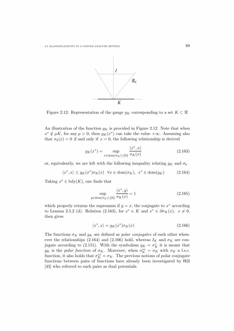
2.5. ELASTOPLASTICITY IN A CONVEX-ANALYTIC SETTING 89
Figure 2.12: Representation of the gauge gK corresponding to a set K ⊂ R
An illustration of the function gK is provided in Figure 2.12. Note that whenx∗ /∈ µK, for any µ > 0, then gK(x∗) can take the value +∞. Assuming alsothat σk(x) = 0 if and only if x = 0, the following relationship is derived
gK(x∗) = supx∈dom(σK )\0
〈x∗, x〉σK(x)
(2.163)
or, equivalently, we are left with the following inequality relating gK and σk
〈x∗, x〉 ≤ gK(x∗)σK(x) ∀x ∈ dom(σK), x∗ ∈ dom(gK) (2.164)
Taking x∗ ∈ bdy(K), one finds that
supy∈dom(σK )\0
〈x∗, y〉σK(x)
= 1 (2.165)
which properly returns the supremum if y = x, the conjugate to x∗ accordingto Lemma 2.5.2 (d). Relation (2.163), for x∗ ∈ K and x∗ ∈ ∂σK(x), x = 0,then gives
〈x∗, x〉 = gK(x∗)σK(x) (2.166)
The functions σK and gK are defined as polar conjugates of each other when-ever the relationships (2.164) and (2.166) hold, whereas IK and σK are con-jugate according to (2.151). With the symbolism gK = σK it is meant thatgK is the polar function of σK . Moreover, when σ∗∗K = σK with σK a l.s.c.function, it also holds that σK = σK . The previous notions of polar conjugatefunctions between pairs of functions have already been investigated by Hill[43] who referred to such pairs as dual potentials.

90 2. ELASTOPLASTICITY
Figure 2.13: Support function D corresponding to the map G shown in Figure2.11
We have the following important result which, in the next section, willallow to state the normality law in a form involving the yield function (for theproof refer to [41]).
Lemma 2.5.4 Let g be nonnegative and convex, with g(0) = 0 and x ∈int(dom(g)) such that g(x) > 0. Set C = z : g(z) ≤ g(x). Then y ∈ NC(x)if and only if there exists a scalar γ ≥ 0 such that y ∈ γ∂g(x).
2.5.2 Basic flow relations of elastoplasticity
With the mathematical instruments introduced in the previous section avail-able, it is possible to re-examine the elastoplastic thermodynamic theory stud-ied hitherto. In particular, adopting the standpoint of convex analysis we areable to derive basic results like the yield function convexity, the normality lawin a more rigorous and more general fashion. As a result the yield surfacesmoothness constraint can be avoided, permitting to obtain a set of alterna-tive forms of the plastic flow law, which become of great importance for theanalysis of the variational problem of elastoplasticity carried out in Chapter3.
For later developments and in view of the previous section notation we

2.5. ELASTOPLASTICITY IN A CONVEX-ANALYTIC SETTING 91
convene to establish the following substitutions
X ←→ set of generalized plastic strain rates
x ←→ P =(ep, ξ
)X ′ ←→ set of generalized stresses
x∗ ←→ S = (σ,χ)
Moreover, it is assumed that K represents a closed set in the space of genera-lized stresses S such that it admits the following representation
K = S : φ(S) ≤ 0
through the yield function φ. As done in Section 2.3.1, we refer the zone forwhich φ < 0 as the elastic domain, while those points of K satisfying φ = 0constitute the yield surface.
With these positions we are able to apply the results on maximal respon-siveness and convex sets to the existence of a convex yield surface. Let us recallTheorem 2.5.3 and consider a maximal responsive map G having as its valuessubsets of X ′. First, it is found by (2.157) that the zero generalized stressis contained within the set of thermodynamic forces S corresponding to zerogeneralized plastic strain rate. Second, relation (2.158) constitutes a general-ization of the maximum plastic work inequality (2.58) in the case of perfectlyplastic materials and, admitting σ0 ∈ G(ep
0) and σ1 ∈ G(ep1), becomes
(σ0 − σ1) : ep0 ≥ 0 and (σ1 − σ0) : ep
1 ≥ 0
that parallels (2.55).Going a step further, we may inquire whether the maximal responsiveness
condition which permits deducing yield surface convexity can be derived as aconsequence of the Principle of maximum plastic dissipation inequality (2.59).Apply Theorem 2.5.3 and Lemma 2.5.2. By the maximal responsiveness condi-tion we are led to recognize the existence of a closed convex set K of admissiblegeneralized stresses and of a generalized normality rule stated in the form
P ∈ NK(S) (2.167)
Theorem 2.5.3, moreover, implies the equivalence between the normality rule(2.167) and the following
S ∈ G(P) (2.168)

92 2. ELASTOPLASTICITY
Since
S ∈ int(K)⇒ NK(S) = 0
it is clear from (2.167) that in the elastic region P = 0. Hence, it is statedthe equivalence between the existence of a convex yield surface satisfying thenormality rule and the property of maximal responsiveness.
At this point it is possible to draw some considerations on the dissipationfunction. The dissipation function D, defined by (2.57) in Section 2.3.1, in thepresent context becomes the function g that appears in Lemma 2.5.2 and ischaracterized by being the support function of the setK. With this associationand inspecting (2.59) we are left with
D(P) = supT : P : T ∈ K = S : P (2.169)
which indicates that S represents the point which returns the supremum ofthe set of admissible plastic work rates.
If we consider the Legendre-Fenchel conjugate D∗ of the function D, thatis the indicator function of the set K; applying Lemma 2.5.2(d), we arrive atthe equivalent condition
S ∈ ∂D(P) (2.170)
which provides the connection existing between the support function D andthe maximal responsive map G through Theorem 2.5.3.
Going back for a moment to the example presented in Figure 2.11 whichshows the support function corresponding toG, we can derived the relationship
G = ∂D (2.171)
The last equation qualifies D as a pseudopotential for S [23].The analytical considerations carried out in Section 2.5.1 make it possible
to derive the following equivalent formulations of the flow law in plasticity
(a) G maximal responsiveS ∈ G(P)
(b) G convex, positively homogeneous, l.s.c.D(P) ≥ 0, D(0) = 0S ∈ ∂D(P)
2.5. ELASTOPLASTICITY IN A CONVEX-ANALYTIC SETTING 93
(c) K closed, convex, containing 0D∗ = indicator function of KP ∈ ∂D∗(S) = NK(S)
Relationship between the yield and dissipation functions
The analysis on polar functions presented in Section 2.5.1 permits to recognizean enlightening relationship between the yield and dissipation function. Equa-tion (2.161) authorizes to define a gauge function g (we omit for brevity thesubscript K with no ambiguity) corresponding to which the set of admissiblegeneralized stress can be expressed as
K = S : g(S) ≤ c0
The above representation of the yield function through a gauge is usuallytermed the canonical yield function. The gauge g is defined according to
g(S) = infµ > 0 : S ∈ µK
and, by generalization, we infer that any yield surface may be represented inthis manner. In the sequel it is be assumed that f represents an arbitraryrepresentation of the yield function, while g refers to the canonical represen-tation.
Assume that the dissipation D(Λ) = 0 (for convenience, we indicate mo-mentarily the argument of D by Λ, a generalized plastic strain rate) if andonly if Λ = 0. It results clear from (2.163) that g and D are related by
g(S) = supΛ∈dom(D)\0
S : ΛD(Λ)
In the case where S ∈ ∂K, the boundary of K, then
supΛ∈dom(D)\0
S : ΛD(Λ)
= 1
The above expression reaches the supremum when Λ = P, being P conjugateto S in the sense of an equality in (2.169). Hence, for S ∈ K ∩ ∂D(P) andP = 0, it holds
S : P = g(S)D(P) (2.172)

94 2. ELASTOPLASTICITY
Figure 2.14: Relationship between the admissible set K and its support func-tion D
by which when D and D∗ are Legendre-Fenchel conjugate, D and g are polarin the sense of (2.172).
The above polarity condition for the canonical form of the yield functiong enables to derive a generalized version of the classical flow rule (2.60), usingLemma 2.5.4. Consider the following
Lemma 2.5.5 Let g be non-negative and convex, with g(0) = 0 and S a pointin the interior of dom(g) such that g(S) > 0. Set K = T : g(T) ≤ g(S).Then P ∈ NK(S) if and only if there exists a constant γ ≥ 0 such that
P ∈ γ∂g(S) (2.173)
Equation (2.60) is readily seen to coincide with (2.173) as soon as g is smooth.Moreover, we can write
P ∈ γ∂g(S)⇔ γg(T) ≥ γg(S) + P : (T− S) ∀T
Considering sequentially the cases T = 0 and T = 2S and using the propertiesof the gauge g, yields the following characterization of the plastic multiplier
γ = D(P)
The above fundamental relation simply qualifies the scalar quantity γ as thedissipation corresponding with a particular generalized plastic strain rate. In-deed, Lemma 2.5.5 also applies to the particular case g = D. Setting
C = Q : D(Q) ≤ D(P)

2.5. ELASTOPLASTICITY IN A CONVEX-ANALYTIC SETTING 95
for P = 0, it is readily found that there exists a strictly positive γ (excludingγ = 0 since S = 0 by hypothesis) such that
S ∈ NC(P) or S ∈ γ∂D(P)
whenever a relation like (2.170) insists between S and P. A clear visualiza-tion of the previous concept can be seen in Figure 2.14 which shows the pair(S, P) ∈ X ′ such that the rate P is in the normal cone to K (the level setg(S) ≤ 1) at S. Instead, it is evident that in X, the point S lies in the normalcone to C (the level set D(Q) ≤ D(P) at P).

96 2. ELASTOPLASTICITY

Chapter 3
Variational Formulation ofthe Elastoplastic EquilibriumProblem
Introduzione
Il presente capitolo e incentrato sulla formulazione variazionale o formulazionedebole del problema a valori iniziali e dati al bordo dell’equilibrio per solididi materiale elastoplastico. Il capitolo e strutturato in maniera da soddisfaredue istanze. La prima e quella di presentare le due classiche formulazioni vari-azionali del problema elastoplastico, cosiddette primale e duale. La secondae quella di fornire, senza addentrarsi eccessivamente nella dimostrazione ma-tematica, i risultati essenziali sulla buona posizione del problema variazionalein discorso. Il capitolo e suddiviso in due sezioni.
La Sezione 3.2 riguarda la cosiddetta formulazione primale del problemadell’equilibrio elastoplastico. La caratteristica di tale formulazione risiede nellaadozione di una particolare forma della legge costitutiva. Detta scelta si ri-flette sul tipo di spazi funzionali su cui il problema e formulato. In partico-lare, le grandezze incognite, secondo la formulazione primale, risultano esserelo spostamento ed il tensore di deformazione plastica generalizzato. In rife-rimento al modello elastoplastico trattato tipo von-Mises, sono presentati irisultati classici di buona posizione del problema primale.
La Sezione 3.3 riguarda la cosiddetta formulazione variazionale duale delproblema dell’equilibrio elastoplastico. Tale problema si dimostra equivalenteal problema in forma primale, eccetto che per la forma della legge costitutivaadottata. Tale scelta induce una posizione del problema su spazi funzionalidifferenti rispetto a quelli su cui e posto il problema in forma primale. In questo
97

98 3. VARIATIONAL FORMULATION OF THE ELASTOPLASTIC EQUILIBRIUM PROBLEM
caso, infatti, le grandezze incognite sono rispettivamente lo spostamento ed iltensore delle tensioni generalizzato.
La forma duale del problema dell’equilibrio elastoplastico rappresenta laversione piu comune di formulazione debole per tale problema riscontrabilein letteratura. Essa costituisce infatti l’oggetto del capitolo successivo che neaffronta la approssimazione numerica.
Le definizioni fondamentali sulle disequazioni variazionali ellittiche e para-boliche e relative proprieta di esistenza ed unicita della soluzione sono breve-mente richiamate nella Appendice B.
La trattazione matematica svolta in questo capitolo trae maggiormentespunto da [41].
3.1 Introduction
The present chapter is devoted to the variational or weak formulation of theinitial boundary value equilibrium problem of elastoplastic material bodies orsimply elastoplastic equilibrium problem. The chapter has two main purposes.The first one is to present the structure of the classical weak formulations ofelastoplastic problems. The second one is to provide the basic results on well-posedness for the above problems. This latter part is carried out withoutgoing into the mathematical details of the theoretical results. The chapter issubdivided in two sections.
Section 3.2 regards the so-called primal variational formulation of theelastoplastic equilibrium problem. The characterizing feature of this formu-lation is the form of the flow rule which is adopted. This choice reflects alsothe spaces on which the problem is posed. Particularly, the unknowns of theproblem are the displacement and the generalized plastic strain. Following[41], we present the fundamental results on the well-posedness of the problemunder consideration for the relevant case of von-Mises plasticity with linearhardening.
Section 3.3 regards the so-called dual variational formulation of the elasto-plastic equilibrium problem. This is by any means the same physical problembut with a different choice of the flow rule. In this way the space on which theproblem is formulated results different than that of the primal formulation.In this case, in fact, the unknowns are respectively the displacement and thegeneralized stress. The results on well-posedness of the dual problem are stillderived from [41] in a very sharp manner. The dual variational problem isprobably the most common version of the elastoplastic equilibrium weak for-mulation and remains of primary importance. Indeed, it is the one which is

3.2. THE PRIMAL VARIATIONAL FORMULATION 99
addressed in the following chapter where its numerical solution is considered.The basic definitions on elliptic and parabolic variational inequalities to-
gether with the elementary properties of existence and uniqueness of solutionused in this chapter are collected briefly in Appendix B.
The mathematical arguments presented in this chapter mainly derive from[41].
3.2 The primal variational formulation
Basic relations
We briefly recollect here all the “ingredients” necessary in order to obtain avariational formulation of the boundary value problem of quasi-static equili-brium for an elastoplastic solid. It is assumed in the following developmentsthat all the governing equations are given on a Lipschitz domain Ω with bound-ary Γ.
The unknown variables of the problem are respectively the displacementvector u, the plastic strain tensor ep and the internal variables ξ. The equa-tions governing the problem in the domain Ω at any instant t ∈ [0, T ] (cf.Section 1.7) are the
• equilibrium equationdivσ + b = 0 (3.1)
• the strain-displacement relation
εεε(u) =12[∇u + (∇u)T
](3.2)
• the constitutive law
σ = C(εεε(u)− ep) (3.3)χ = −Hξ (3.4)
with the flow rule and the maximum plastic dissipation inequality in the form(cf. (2.167) and (2.58))
(ep, ξ) ∈ Kp
D(q,η) ≥ D(ep, ξ) + σ : (q− εεε) + χ : (η − ξ) ∀(q,η) ∈ Kp
(3.5)
where Kp = dom(D) (1). The dissipation D, due to the considerations madein the previous chapter, is a gauge, i.e. it is a nonnegative, convex, positivelyhomogeneous and l.s.c. function with D(0) = 0.
1For a detailed derivation of the expression (3.5)2 refer to [41]

100 3. VARIATIONAL FORMULATION OF THE ELASTOPLASTIC EQUILIBRIUM PROBLEM
Material parameters
Some assumptions on the material parameters are necessary for the well posed-ness of the problem and to assure a realistic representation of elastoplasticmaterials.
The elastic tensor C has the following symmetries
Cijkl = Cjikl = Cklij (3.6)
and it is pointwise stable, that is, for some constant C0 > 0 it holds
ζ : C(x)ζ ≥ C0 ‖ ζ ‖2 ∀ζ ∈ Linsym, a.e. in Ω (3.7)
For obvious reasons, C has bounded and measurable components,
Cijkl ∈ L∞(Ω) (3.8)
The hardening moduli matrix H, which can be viewed as a linear operatorfrom the space of the internal variables ξ into itself (cf. 2.95), is taken to besymmetric in the sense that
ξ ·Hλ = λ ·Hξ (3.9)
for any couple of vectors of internal variables ξ and λ. Finally, we admit thatH has bounded and measurable components which satisfy
Hij ∈ L∞(Ω) (3.10)
and it is positive definite, in the sense that there exists a constant H0 suchthat
ξ ·Hξ ≥ H0 ‖ ξ ‖2 (3.11)
for all the vectors of internal variables ξ = (ξk) s.t. ξk ∈ Linsym, (1 ≤ k ≤ m).In addition, we admit that the compliance tensor C
−1 exists, it possesses thesame symmetry properties as C and it is also pointwise stable. This impliesthat there exists a constant C0 such that
ζ : C−1(x)ζ ≥ C0 ‖ ζ ‖2 ∀ζ ∈ Linsym, a.e. in Ω (3.12)
Indeed, the inverse H−1 of the hardening moduli matrix exists and it shares
the same properties of H, i.e. it is symmetric, it has bounded measurablecomponents and it satisfies the pointwise stability property:
ξ ·H−1ξ ≥ H ′0 ‖ ξ ‖2 (3.13)
for all the vectors ξ.

3.2. THE PRIMAL VARIATIONAL FORMULATION 101
Initial and boundary conditions
For brevity, we only consider homogeneous Dirichlet-type boundary conditionsfor the problem under consideration. This choice does not affect the generalityof treatment by any means and the results presented in the following sectionscan readily be extended to mixed type of boundary conditions [41]. Hence, weassume that
u = 0 on Γ (3.14)
The initial condition on the displacement is of the form
u(x, 0) = 0 in Ω (3.15)
Function spaces
The variables of the problem need be collocated within appropriate functionspaces. Accordingly, we define the space of admissible displacements by
V =[H1
0 (Ω)]3
The space of plastic strains is taken as
Q0 = q ∈ Q : tr(q) = 0 a.e. in Ω
a closed subspace of the space Q defined by
Q =q : q ∈ Linsym, qij ∈ L2(Ω)
The space Q is endowed with the inner product and the norm of the space[L2(Ω)]3×3. We have then the space M of internal variables, defined by
M =η = (ηk) : ηk ∈ Linsym, ηk|ij ∈ L2(Ω), 1 ≤ k ≤ m
which is endowed with the usual L2(Ω)-based inner product and norm.
The statement of the problem makes use of the following space
Z = V ×Q0 ×M
which becomes a Hilbert space with the inner product
(w, z)Z = (u,v)V + (ep,q)Q + (ξ,η)M
and the norm ‖ z ‖Z= (z, z)1/2Z , where w = (u, ep, ξ) and z = (v,q,η). Letting
Kp = dom(D), it is also defined the set
Zp = z = (v,q,η) ∈ Z : (q,η) ∈ Kp a.e. in Ω (3.16)
which is a nonempty, closed, convex cone in Z.

102 3. VARIATIONAL FORMULATION OF THE ELASTOPLASTIC EQUILIBRIUM PROBLEM
Bilinear form and functionals
We introduce the bilinear form a : Z × Z → R, defined by
a(w, z) =∫
Ω[C(εεε(u)− ep) : (εεε(v)− q) + ξ ·Hη] dv (3.17)
the linear functional (t) : Z →R given by
〈(t), z〉 =∫
Ωb · vdv (3.18)
and the functional j : Z →R such that
j(z) =∫
ΩD(q,η)dv (3.19)
where w = (u, ep, ξ) and z = (v,q,η).Due to the symmetry properties of C and H, the bilinear form a(·, ·) is
symmetric as well. By the definition and properties of the dissipation D,the functional j(·) is a convex, positively homogeneous, nonnegative and l.s.c.functional. It is noted that in general j is not differentiable.
Primal formulation
First, integrating relation (3.5)2 over the domain Ω and substituting in theensuing integral inequality respectively (3.3) and (3.4) we obtain∫
ΩD(q,η)dv ≥
∫ΩD(ep, ξ)dv +
∫Ω
[C (εεε(u)− ep) : (q− ep)−Hξ · (η − ξ)
]dv
∀(q,η) ∈ Zp
(3.20)
Next, taking the scalar product of relation (3.1) with v − u for an arbitraryv ∈ V , integrating over Ω and performing sequentially an integration by partsand the substitution of expression (3.3) for the stress σ, we arrive at thefollowing equation∫
ΩC [εεε(u)− ep] : [εεε(v)− εεε(u)] dv =
∫Ω
b · (v− u)dv ∀v ∈ V (3.21)
Summing relations (3.20) and (3.21), we obtain the variational inequality
a(w(t), z − w(t)) + j(z)− j(w(t)) ≥ 〈(t), z − w(t)〉 (3.22)

3.2. THE PRIMAL VARIATIONAL FORMULATION 103
which holds on the space Zp. Formally, the primal variational formulation ofthe elastoplastic initial boundary value problem of equilibrium can thus bestated as [41]
Problem Prim. Given a linear functional ∈ H1(0, T ;Z ′), (0) = 0, findw = (u, ep, ξ) : [0, T ] → Z, w(0) = 0, such that for almost all t ∈ (0, T ),w ∈ Zp and
a(w(t), z − w(t)) + j(z)− j(w(t)) ≥ 〈(t), z − w(t)〉 ∀z ∈ Zp (3.23)
It is noted that if w is a classical solution of the problem defined by (3.1)-(3.5)and (3.14)-(3.15), then it is a solution of the problem Prim (See Appendix B).Conversely, inverting the developments which leads to the inequality (3.23) itis possible to recognize that if w is a smooth solution to problem Prim, thenit is also a classical solution of the problem posed in local form. Hence thetwo formulation are formally equivalent.
For the applicability of theoretical results in the analysis of the initialboundary value problem in argument, it is more convenient to view the in-equality (3.23) as one posed on the whole space Z, instead than on its sub-space Zp. Recalling that j(z) =∞ when z /∈ Zp and invoking the requirementw ∈ Zp, (3.23) can be rewritten equivalently in the form
a(w(t), z− w(t)) + j(z)− j(w(t)) ≥ 〈(t), z− w(t)〉 ∀z ∈ Z (3.24)
The subdifferential of j(·) is defined as
∂j(w) =w∗ ∈ Z ′ : j(z) ≥ j(w) + 〈w∗, z− w〉 ∀z ∈ Z
(3.25)
and with the aid of (3.24) it is possible to restate the original problem (3.23)as an equation and an inclusion. Setting the new auxiliary variable w∗, we arelead to the new problem of finding a couple of functions w : [0, T ] → Z andw∗ : [0, T ]→ Z ′ satisfying, for almost all t ∈ (0, T ) the following relations
a(w(t), z) + 〈w∗(t), z〉 = 〈(t), z〉 ∀z ∈ Z (3.26)w∗(t) ∈ ∂j(w(t)) (3.27)
Consequently, noting that j is positively homogeneous, it follows that Equation(3.27) is equivalent to the couple of conditions
〈w∗(t), z〉 ≤ j(z) ∀z ∈ Z (3.28)
and
〈w∗(t), w(t)〉 = j(w(t)) (3.29)

104 3. VARIATIONAL FORMULATION OF THE ELASTOPLASTIC EQUILIBRIUM PROBLEM
Ultimately, we can see that, setting to zero all the above plastic and hardeningvariables appearing in the formulation of problem Prim, one is left with thefollowing variational equation∫
ΩCεεε(u) : εεε(v)dv =
∫Ω
b · vdv ∀v ∈[H1
0 (Ω)]3
which recovers exactly the boundary value problem of linear elasticity (B.14)examined in Appendix B, i.e.∫
ΩCεεε(v) : εεε(v)dv =
∫Ω
b · vdv ∀v ∈[H1
0 (Ω)]3
with Dirichlet homogeneous boundary conditions on the whole boundary.
Combined linear kinematic and isotropic hardening with von-Misesyield function
We now address the formulation of the problem Prim in the special case ofcombined linear kinematic and isotropic hardening with the von-Mises yieldfunction. In this context the unknowns of the problem can be identified bythe triplets u, ep, ep, namely the displacement, the plastic strain and the ac-cumulated plastic stain. The spaces V and Q0 remain unchanged, while thespace of internal variables M reduces to L2(Ω). With this position, we maywrite the admissible set Zp as
Zp = z = (v,q, µ) ∈ Z : ‖ q ‖≤ µ a.e. in Ω
The bilinear form a(·, ·) : Z × Z →R becomes
a(w, z) =∫
Ω[C(εεε(u)− ep) : (εεε(v)− q) +Hkinep : q +Hisoe
pµ] dv (3.30)
where, obviously, w = (u, ep, ep) and z = (v,q, µ). The functional j is definedaccording to (3.19) and reads
j(z) =∫
ΩD(q, µ)dv
whilst the dissipation D, in the case of the von-Mises yield criterion, can beexpressed in the following alternative form (cf. (2.102) and refer to [41] for adetailed explanation of this expression)
D(q, µ) =
c0 ‖ q ‖ if ‖ q ‖≤ µ
+∞ if ‖ q ‖> µ(3.31)

3.2. THE PRIMAL VARIATIONAL FORMULATION 105
The linear functional (t) simply remains as in (3.18). The above specifica-tions produce the following formulation of the problem with combined linearkinematic-isotropic hardening [41].
Problem Prim1. Given a linear functional ∈ H1(0, T ;Z ′), (0) = 0, findw = (u, ep, ep) : [0, T ]→ Z, with w(0) = 0, such that for almost all t ∈ (0, T ),w ∈ Zp and
a(w(t), z − w(t)) + j(z)− j(w(t)) ≥ 〈(t), z − w(t)〉 ∀z ∈ Zp (3.32)
The problem just formulated, being a special case, shares with its generalcounterpart Problem Prim. all of its properties, in particular it resultsequivalent to its local form.
Linear kinematic hardening with von-Mises yield function
The elastoplastic problem of a material experiencing purely linear kinematichardening and characterized by a von-Mises type yield function can be for-malized as a degenerate case of Problem Prim1, with Hiso = 0. The solutionspace is now simply Z = V ×Q0 with the inner product
(w, z)Z = (u,v)V + (ep,q)Q
and the usual norm ‖ z ‖Z= (z, z)1/2Z . Here, w = (u, ep) and z = (v,q). The
dissipation function D becomes
D = c0 ‖ q ‖ ∀q ∈ Q0
so that the function
j(z) =∫
ΩD(q)dv for z = (v,q) ∈ Z
is finite on the entire space Z. The bilinear form is now
a(w, z) =∫
Ω[C(εεε(u)− ep) : (εεε(v)− q) +Hkinep : q] dv (3.33)
The linear functional (t) is still given by (3.18). The statement of the initialboundary value problem is then
Problem Prim2. Given a linear functional ∈ H1(0, T ;Z ′), (0) = 0, findw = (u, ep) : [0, T ] → Z, with w(0) = 0, such that for almost all t ∈ (0, T ),w ∈ Zp and
a(w(t), z− w(t)) + j(z)− j(w(t)) ≥ 〈(t), z− w(t)〉 ∀z ∈ Z (3.34)
106 3. VARIATIONAL FORMULATION OF THE ELASTOPLASTIC EQUILIBRIUM PROBLEM
Existence, uniqueness and stability of the primal formulation
In this short section we aim to give a hint at the properties of existence,uniqueness and stability of the solutions to the variational problems givenhitherto in the so called primal formulation. For brevity’s sake the proofs ofthe properties herein exposed are not presented and the reader is referred againto [41] for the complete derivation of results. Following [41], it is seen thatthe proper way to study the primal variational formulation of the elastoplasticequilibrium problem is that of recasting the ensuing variational inequality intoa more general framework which may be stated as follows:
Problem ABS. Find w : [0, T ] → H, w(0) = 0, such that for almost allt ∈ (0, T ), w(t) ∈ K and
a(w(t), z − w(t)) + j(z) − j(w(t)) ≥ 〈(t), z − w(t)〉 ∀z ∈ K (3.35)
where H denotes a Hilbert space and K a nonempty, closed, convex cone inH. As can be checked in Appendix B, (3.35) is a variational inequality of themixed kind because it shows peculiarities of both variational inequalities ofthe first kind (convex set K on which the test functions are taken) and of thesecond kind (nondifferentiable term j).
The suitable hypotheses under which the above problem shows unique solv-ability and stability have been studied by Han, Reddy and Schroeder [42] forthe elastoplastic problem with combined linear isotropic and kinematic harden-ing. These hypotheses concern, respectively, the bilinear form a(·, ·) which isrequired to be H-elliptic and the functional which must be a H1(0, T ;H ′),function with j(0) = 0. Moreover, the functional j is required to be nonneg-ative, convex, positively homogeneous and Lipschitz continuous (even if notnecessarily differentiable). When the above conditions are fulfilled, it is possi-ble, with some mathematical manipulations, to show that the original abstractvariational inequality (3.35) is equivalent to
a(w(t), z − w(t)) + j(z) − j(w(t)) ≥ 〈(t), z − w(t)〉 ∀z ∈ H
The preceding relation implies that it is possible to choose the test functions zin H instead of K. In this way, Theorem B.2.3, the standard solvability result,is applicable.
We are now in a position to introduce the following fundamental resultwhich plays a key role in the subsequent specializations of the abstract pro-blem in argument to its elastoplasticity counterpart in the vest of the primalformulation. Under a proper set of fundamental assumptions on the bilinearform a and on the linear functional it results possible to state general results
3.2. THE PRIMAL VARIATIONAL FORMULATION 107
of existence, uniqueness and stability of the solution to the problem Abs. As aspecial case we may have the problem Prim and its specializations Prim1 andPrim2. It is therefore possible to extend the results on the abstract problemto the practical elastoplastic problems examined hitherto.
Theorem 3.2.1 Existence and Uniqueness of Problem Abs. [41] LetH a Hilbert space; K ⊂ H a nonempty, closed, convex cone; a : H ×H → Ra bilinear form that is symmetric, bounded and H-elliptic; ∈ H1(0, T ;H ′)with (0) = 0 and j : K → R a nonnegative, convex, positively homogeneousand Lipschitz-continuous function. Then, there exists a unique solution w ofProblem Abs satisfying w ∈ H1(0, T ;H). Furthermore, w : [0, T ] → H is thesolution to problem Abs if and only if there is a function w∗(t) : [0, T ] → H ′
such that for almost all t ∈ (0, )
a(w(t), z) + 〈w∗(t), z〉 = 〈(t), z〉 ∀z ∈ H (3.36)w∗(t) ∈ ∂j(w(t)) (3.37)
Following [41] we are also provided of the following stability result
Theorem 3.2.2 Stability of Problem Abs. [41] Under the assumptionsof Theorem 3.2.1, the solution of Problem Abs depends continuously on . Inparticular, given two linear functionals (1), (2) ∈ H1(0, T ;H ′) with (1)(0) =(2)(0) = 0, the corresponding solutions w(1) and w(2) are related by the fol-lowing estimate
‖ w(1) − w(2) ‖L∞(0,T ;H)≤ c ‖ (1) − (2) ‖L1(0,T ;H′) (3.38)
The preceding theorems permit to extend the results made clear for the ab-stract variational problem (3.35) to the physical problem under consideration,i.e. the primal variational formulation Prim together with its particular casesPrim1 and Prim2. Relatively to the definition (3.17), we first note that ingeneral the bilinear form a(·, ·) cannot be expected to be Z-elliptic, since
a(z, z) =∫
Ω[C(εεε(v)− q) : (εεε(v)− q) + η ·Hη] dv
for z = (v,q,η) ∈ Z and since it is at most
a(z, z) ≥ c(‖ εεε(v)− q ‖2[L2(Ω)]3×3 + ‖ η ‖2[L2(Ω)]m
)On the other hand, the variational inequality (3.23) is posed on the set Zp,defined by (3.16) and the requirement z ∈ Zp produces a constraint on the

108 3. VARIATIONAL FORMULATION OF THE ELASTOPLASTIC EQUILIBRIUM PROBLEM
relation between the components q and η. We are then lead to make thefollowing assumption
z = (v,q,η) ∈ Kp ⇒ β ‖ q ‖2≤ η ·Hη for some constant β > 0 (3.39)
This crucial assumption can be shown, with an application of the Korn’s in-equality, to make the bilinear form a(·, ·) Z-elliptic on Zp [41], in the sensethat there exists a constant c0 > 0 such that
a(z, z) =∫
Ω[C(εεε(v)− q) : (εεε(v)− q) + η ·Hη] dv ≥
c0(‖ v ‖2V + ‖ q ‖2Q + ‖ η ‖2M
) (3.40)
The last result is of great importance since in the practical cases analyzedpreviously the assumption (3.39) is satisfied. Thus we have the followingresult.
Theorem 3.2.3 [41] Under the assumption (3.39), the problem Prim has asolution
The proof of this last statement, which is omitted here for brevity’s reasons,parallels the existence proof of the abstract problem (3.35), but makes use ofProposition B.1.2, instead of Theorem B.2.3, which results unapplicable heresince the bilinear form is not elliptic on the whole space.
In conclusion, it is to be pointed out that lacking the ellipticity of a(·, ·)over the whole space Z, uniqueness and stability of a problem solution cannotbe proved. In the two particular cases seen above regarding combined linearisotropic and kinematic hardening and of pure linear kinematic hardening, itis found that the bilinear form ellipticity is granted on the entire space Z.The remainder of this section is devoted to important results valid in such twosituations. We have then the following theorems
Theorem 3.2.4 Existence and Uniqueness - Problem Prim1. [41] Un-der the assumptions made on the data for Problem Prim, the quasi-staticelastoplastic equilibrium problem Prim1 has a unique solution w = (u, ep, ep) ∈H1(0, T ;Z). Furthermore, if w(1) and w(2) are the solutions corresponding to(1), (2) ∈ H1(0, T, Z ′), with (1)(0) = (2)(0) = 0, then the following estimateholds
‖ w(1) −w(2) ‖L∞(0,T ;Z)≤ c ‖ (1) −
(2) ‖L1(0,T ;Z′) (3.41)
A similar result holds for the other special case of the primal problem. Indeed,we have

3.3. THE DUAL VARIATIONAL FORMULATION 109
Theorem 3.2.5 Existence and Uniqueness - Problem Prim2. [41] Un-der the assumptions made on the data for Problem Prim, the quasi-staticelastoplastic equilibrium problem Prim2 has a unique solution w = (u, ep) ∈H1(0, T ;Z). Furthermore, if w(1) and w(2) are the solutions corresponding to(1), (2) ∈ H1(0, T, Z ′), with (1)(0) = (2)(0) = 0, then the following estimateholds
‖ w(1) −w(2) ‖L∞(0,T ;Z)≤ c ‖ (1) −
(2) ‖L1(0,T ;Z′) (3.42)
3.3 The dual variational formulation
The variational formulation examined in this section makes use of the flow lawin the form (2.167). This choice leads to a problem in which the unknownvariables are the displacement vector u and the generalized stress vector S =(σ,χ). We begin, as done in Section 3.2 with the proper space setting of thefields involved in the formulation. The space of admissible displacement is stillindicated by
V =[H1
0 (Ω)]3
while the space of stresses is defined as
S =τ : τ ∈ Linsym, τij ∈ L2(Ω)
The space of conjugate forces is given by
M =µ = (µk) : µk ∈ Linsym, µk|ij ∈ L2(Ω), 1 ≤ k ≤ m
For later purposes, we set
T = S ×M
and implicitly endow this space with the inner products naturally inducedby the inner products defined respectively on S and M . Recalling that theadmissible generalized stresses are those belonging to the set K pointwise, wemay define the following convex subset
P = T = (τ ,µ) ∈ T : (τ ,µ) ∈ K a.e. in (Ω) (3.43)
We are now in a position to introduce the following bilinear forms which definethe elastoplastic dual problem
a : S × S →R, a(σ, τ ) =∫
Ωσ : C
−1τdv (3.44)

110 3. VARIATIONAL FORMULATION OF THE ELASTOPLASTIC EQUILIBRIUM PROBLEM
b : V × S →R, b(v, τ ) = −∫
Ωεεε(v) : τdv (3.45)
c : M ×M →R, c(χ,µ) =∫
Ωχ ·H−1µdv (3.46)
together with the bilinear form
A : T × T → R, A(S,T) = a(σ, τ ) + c(χ,µ) (3.47)
with S = (σ,χ) and T = (τ ,µ). It is remarked that both the compliancetensor C
−1 and the inverse of the hardening moduli operator H−1 possess the
same material properties of symmetry, pointwise stability and boundednessstated in the previous section. Moreover, in view of the above properties, thebilinear form A(·, ·) results symmetric, continuous and T -elliptic, i.e. thereexist two positive constants αA and βA such that
|A(S,T)| ≤ αA ‖ S ‖T ‖ T ‖T ∀S,T ∈ T (3.48)A(T,T) ≥ βA ‖ T ‖2T ∀T ∈ T (3.49)
The bilinear form b(·, ·) is continuous or equivalently, there exists a positiveconstant αb such that
|b(v, τ )| ≤ αb ‖ v ‖V ‖ τ ‖S ∀v ∈ V, τ ∈ S (3.50)
Moreover, for some constant βb > 0, it holds
supτ∈S\0
|b(v, τ )|‖ τ ‖S
≥ βb ‖ v ‖V ∀v ∈ V (3.51)
The above bound can be easily proved taking τ = εεε(v) and applying Korn’sinequality (A.18). The linear functional of the load is as usual defined by
(t) : V →R, 〈(t),v〉 = −∫
Ωb(t) · vdv (3.52)
It is then possible to derive the dual formulation of the elastoplastic problemby applying the standard procedure and recalling, respectively, the local formof the equilibrium equation
div σ + b = 0 in Ω
and the flow law in the form
(σE − σ) : C−1(τ − σ)− χ ·H−1(µ− χ) ≤ 0 ∀(τ ,µ) ∈ K

3.3. THE DUAL VARIATIONAL FORMULATION 111
derived from (2.167) in which σE = Cεεε(u) is the elastic stress rate. Thevariational statement reads as follows:
Problem Dual. Given a linear functional ∈ H1(0, T ;V ′), with (0) = 0,find (u,S) = (u,σ,χ) : [0, T ] → V × P, with (u(0),S(0)) = (0,0), such thatfor almost all t ∈ (0, T )
b(v,σ(t)) = 〈(t),v〉 ∀v ∈ V (3.53)A(S(t),T − S(t)) + b(u(t), τ − σ(t)) ≥ 0 ∀T = (τ ,µ) ∈ P (3.54)
The formal equivalence of Problem Dual to the classical problem can be easilyestablished. It is also immediate to show that the above problem, setting tozero all the elastoplastic internal forces χ and letting σ, τ ∈ S, reduces to thelinear elastic initial boundary value equilibrium problem (B.20)-(B.21) withhomogeneous displacement boundary conditions.
The issue of proving existence and uniqueness of the solution of the dualform is addressed in detail in [41]. Here, for brevity, we give just a brief clueof the concepts necessary to pose such a result.
First, we may observe that the bilinear form b(·, ·) : V ×S →R, appearingin (3.53) and defined by (3.45), satisfies the Babuska-Brezzi condition by meansof (3.51). Hence, this bilinear form induces two bounded linear operatorsB : S → V ′ and B′ : V → S′ defined as
b(v, τ ) = 〈Bτ ,v〉 = 〈B′v, τ 〉 for v ∈ V, τ ∈ S (3.55)
The above properties lead to the following
Lemma 3.3.1 The operator B defined by the bilinear form b(·, ·) through re-lation (3.55) is an isomorphism from (KerB)⊥ onto V ′ and the operator B′ isan isomorphism from V onto (KerB), where
KerB = τ ∈ S : b(v, τ ) = 0 ∀v ∈ V (KerB) = f ∈ S′ : 〈f, τ 〉 = 0 ∀τ ∈ KerB
Thus, we have the following important equivalence result
Theorem 3.3.2 Assume b ∈ H1(0, T ;V ′). Then (u, ep, ξ) ∈ H1(0, T ;Z) is asolution of the problem Prim if and only if (u,σ,χ) ∈ H1(0, T ;V × T ) is asolution of the problem Dual, where (u, ep, ξ) and (u,σ,χ) are related by the(constitutive) equations
σ = C(εεε(u)− ep)χ = −Hξ

112 3. VARIATIONAL FORMULATION OF THE ELASTOPLASTIC EQUILIBRIUM PROBLEM
or
ep = εεε(u)−C−1σ
ξ = −H−1χ
The well-posedness of the dual variational formulation of the elastoplasticproblem is then inferred by that of the primal problem.
If we are not to follow this route for proving well-posedness of ProblemDual, we can instead follow another argument which can be regarded as inde-pendent of the developments carried out with respect to the primal formulationto the equivalence result, Theorem 3.3.2. Again, in the same fashion adoptedfor the primal version of the elastoplastic variational problem, some aprioriassumptions have to be taken, in order to show existence and uniqueness “abinitio”. The first assumption concerns the set P and requires that there existsa constant c > 0 such that for any generalized stress S1 = (σ1,χ1) ∈ P andany σ2 ∈ S, it corresponds a χ2 ∈M which satisfies
‖ χ2 ‖≤ c ‖ σ2 ‖ and S1 + S2 ∈ Pwith S2 = (σ2,χ2). This assumption is satisfied in practical situations asthat of combined linear isotropic and kinematic hardening. With some math-ematical manipulations and recalling Lemma 3.3.1, it is found that the aboveassumptions grants nonemptyness, convexity and closedness of the set P(t).The previous requirement is accompanied by an hypothesis on the structureof the set K, whose definition is recalled here for convenience
K = S ∈ S ×M : φ(S) ≤ 0It is then assumed that for any S ∈ K and any scalar κ ∈ [0, 1), it follows thatκS ∈ K and
infx∈Ω
dist(κS(x), ∂K) > 0
The last statement is satisfied for materials characterized by combined lin-ear isotropic and kinematic hardening as soon as the function φ is positivelyhomogeneous and Lipschitz continuous.
Under the above assumptions, the following result [41] holds true.
Theorem 3.3.3 [41] The variational problem Dual has a unique solution(u,S), with u ∈ H1(0, T ;V ) and S ∈ H1(0, T ;T ).
Remark 3.3.4 The cases of the primal and dual variationals formulation fora constitutive model including nonlinear kinematic hardening are omitted herefor brevity. The same results on existence, uniqueness and stability apply alsoto such cases and can be deduced with similar reasonings starting from theprinciple of maximum dissipation (see, for instance, [4, 69, 70, 79]).

Chapter 4
Discrete VariationalFormulation of theElastoplastic EquilibriumProblem
Introduzione
Il tema trattato dal presente capitolo riguarda la risoluzione del problemavariazionale dell’equilibrio elastoplastico in forma duale attraverso un metodonumerico. Nella letteratura scientifica e possibile trovare, per diversi casi par-ticolari del problema in discorso, soluzioni in forma chiusa [57]. Si osserva,tuttavia, che tali casi riguardano geometrie regolari, condizioni al bordo es-tremamente semplici e comportamento del materiale di tipo semplificato. Equindi evidente che tali situazioni risultano di minore interesse pratico. Lasoluzione approssimata per via numerica, per problemi inerenti modelli mag-giormente aderenti al vero, ovvero meno semplificati, risulta quindi la via daseguire onde ottenere risultati ingegneristicamente significativi.
Un notevole impulso alla ricerca in questo senso e venuto anche dallosviluppo di calcolatori elettronici sempre piu potenti.
L’approssimazione del problema in esame implica, come ben noto, sia unadiscretizzazione rispetto alla variabile spaziale che una discretizzazione tem-porale. Nel seguito del capitolo, maggiore attenzione e rivolta al secondopunto, dato che questo costituisce l’argomento fondamentale di questo lavoro.Nell’immediato vengono presentati brevemente i concetti generali riguardantiil primo tipo di discretizzazione spaziale per mezzo del metodo degli elementi
113

114 4. DISCRETE VARIATIONAL FORMULATION OF THE ELASTOPLASTIC EQUILIBRIUM PROBLEM
finiti. Questo permette di introdurre la terminologia standard dell’analisi perelementi finiti senza entrare nel dettaglio degli aspetti matematici inerenti taletecnica numerica applicata alla Meccanica dei solidi. La scelta emerge dallanecessita di introdurre alcuni concetti di base della discretizzazione spaziale,che vengono richiamati brevemente nella trattazione relativa alla discretiz-zazione temporale che constituisce l’argomento principale di questo capitolo.
Nella Sezione 4.2 viene presentata la discretizzazione spaziale e temporaledel problema elastoplastico posto in forma duale, insieme ai risultati inerentil’esistenza della soluzione per il problema cosı approssimato ed inerenti laconvergenza del metodo numerico. Nella Sezione 4.3 vengono introdotti alcunitra i piu comuni schemi di integrazione temporale basati rispettivamente sullaformula di Eulero all’indietro e sulla formula generalizzata di punto medio. Glischemi di integrazione temporali, specializzati al caso del legame costitutivoelastoplastico in esame, generano una famiglia di metodi che possono esserecaratterizzati come metodi alle differenze finite. In relazione a tali metodi sonopresentati i principali risultati inerenti stabilita e ordine di accuratezza.
Nella Sezione 4.4 vengono infine proposti due classici algoritmi risolutoridel problema elastoplastico nella forma discretizzata rispetto alla variabiletemporale. I due algoritmi in esame sono basati sullo schema a doppio passodenominato “predictor-corrector” (previsione-correzione). Il primo adotta unpasso di previsione semplicemente elastico, mentre il secondo adotta un passodi previsione tangente.
Il presente capitolo trae spunto principalmente da [41, 70].
4.1 Introduction
The subject of this chapter is the numerical solution of the elastoplastic equili-brium boundary value problem posed in the dual weak form (see Section 3.3).In the literature it is possible to find a number of solutions to such a problemin closed form (see for instance [57]). It is noted, however, that these situ-ations involve only extremely simple cases consisting of highly regular bodyshape, simple boundary conditions and idealized material behavior. Modelsthat approximate the behavior of real bodies are mostly feasible for approxi-mate solutions which, especially in the recent past, have increasingly becomethe focus of research due to the development of high-speed digital computers.
As it is well known, the approximation of the problem under considerationinvolves both a space discretization issue and a time discretization issue. Inwhat follows we focus the discussion on the second issue, since it constitutesthe central theme of this work. In the immediate following a brief hint of

4.1. INTRODUCTION 115
what concerns the first discretization issue is proposed, referring to one ofthe most commonly used tool in this context: the finite element method.This is done in order to provide the minimum necessary familiarity with thestandard terminology of finite element analysis without entering into a detailedpresentation of the mathematical aspects of the finite element technique inMechanics of solids. This choice emerges from the necessity of having a basicknowledge of the space discretization when dealing with the time discretizationissue which remains the centre of this chapter
In Section 4.2 the space and time (fully) discretization of the dual weakform of the elastoplastic equilibrium is presented and general results on ex-istence of the solution and on convergence are provided. In Section 4.3 weintroduce the most common time integration schemes based on the backwardEuler’s rule and on the generalized midpoint rule. The integration rules arespecialized to the case under consideration stemming into a family of inte-grators which may be grouped into a set of finite difference-based methods.Results on stability and order of convergence are also given. In Section 4.4 wepropose two solution algorithms for the discrete variational formulation of theelastoplastic dual problem based on the predictor-corrector philosophy. Thefirst one adopt a purely elastic predictor, while the second one, the Newton’smethod, adopts a tangent predictor.
The present chapter basically follows the treatment of [41, 70].
4.1.1 Basics of the finite element method
In the following sections we deal with different general solution strategies ofthe elastoplastic equilibrium problem. As it will be made more evident, a keypoint of such strategies is the spatial discretization of the weak formulation ofthe problem. This is assumed to be carried out by the finite element method.Accordingly, since this part of the problem discretization does not representthe center of our discussion, it proves useful to provide some basic notionson the method together with some elementar terminology. This is indeed thetarget of this paragraph. By no means this introductory excursion claims to bemathematically rigorous or theoretically exhaustive and the interested readeris referred to fundamental standard books on the argument.
The development of a finite element scheme for solving an initial boundaryvalue problem involves four main steps. First, the boundary value problem isreformulated into an equivalent variational problem. Second, the domain of theindependent variables (or usually the spatial variables, for a time-dependentproblem as the one under consideration) is partitioned into subdomains calledfinite elements and then a finite-dimensional space, called the finite element

116 4. DISCRETE VARIATIONAL FORMULATION OF THE ELASTOPLASTIC EQUILIBRIUM PROBLEM
space, is constructed as a collection of piecewise smooth functions with a cer-tain degree of global smoothness. Third, the variational problem is projectedto the finite element space and in this way a finite element system is formed.Finally, the solution of the system is searched, say with a proper iterativemethod, and various consideration are drawn from the solution of the finiteelement system.
The mathematical theory of the finite element method addresses manyother issues such as a priori and a posteriori error estimation, convergence,stability and so on. Here we are not interested in entering within such details.With the following lines we simply aim to introduce basic notations and op-erational aspects that will be recalled in the later developments regarding thetime discretization issue. A reader familiar with the basic terminology andtheoretical results of the finite element method may skip this section in toto.For detailed information on the finite element method the reader may refer tothe standard textbooks and among others [19, 26, 48, 62, 79].
Let us now consider, as an example, the finite element method discretiza-tion of the weak formulation associated to a linear elliptic boundary valueproblem defined on a Lipschitz domain Ω:
u ∈ V, a(u, v) = 〈, v〉 ∀v ∈ V (4.1)
where V is a Sobolev space on Ω. For a second-order differential equation pro-blem, V = H1(Ω) if the given boundary condition is natural and V = H1
0 (Ω)if the homogeneous Dirichlet boundary condition is specified over the wholeboundary. As it is shown in Appendix B, a problem with a nonhomogeneousboundary Dirichlet condition on a part of the boundary ΓD ⊂ ∂Ω can be con-verted to one with the homogeneous Dirichlet boundary condition on ΓD aftera change of the dependent variable. In this case, then, the space V = H1
ΓD(Ω).
The form a(·, ·) is assumed to be bilinear, continuous, V -elliptic, while is agiven linear continuous operator on V .
Since V is infinite-dimensional, it is usually impossible to find the solutionof the problem (4.1) in closed form. The idea of the Galerkin method is toapproximate the weak formulation expressed by (4.1) by its discrete analogue
uN ∈ VN , a(uN , v) = 〈, v〉 ∀v ∈ VN (4.2)
where VN ⊂ V is a finite-dimensional space and is used to approximate thespace V . When VN consists of piecewise polynomials associated with a parti-tion of the domain Ω, the Galerkin method (4.2) becomes the classical Galerkinfinite element method.

4.1. INTRODUCTION 117
Convergence of the finite element method may be achieved by progressivelyrefining the mesh or by increasing polynomial degrees or by doing both simul-taneously: then we get the h-version, the p-version or the h-p-version of thefinite element method, respectively. It is customary to use h as the parame-ter for the mesh-size and p as the parameter for the polynomial degree. Anefficient selection among the three versions of the method depends on the apriori knowledge about the regularity of the exact solution of the problem.
In the following sections we consider only the h-version of the method,mainly because the solution of an initial boundary value problem of equilibriumin elastoplasticity does not show high regularity. Conventionally, for the h-version finite element method, we use V h instead of VN to denote the finiteelement space. Thus, with a finite element space V h chosen, the finite elementmethod is
uh ∈ V h, a(uh, vh) = 〈, vh〉 ∀v ∈ V h (4.3)
Expressing the trial function uh in terms of a basis of the space V h and takingeach of the basis functions for the test function vh, we obtain an equivalentlinear system, called the finite element system, from (4.3) for the coefficients inthe expansion of uh with respect to the basis. Once the finite element systemis solved, we can resort to the finite element solution uh.
The quality of the finite element solution uh, i.e. the degree of accuracy inthe approximation of the exact solution u granted by uh relies on the regularityof the exact solution u, the construction of the finite element space V h andeventually on the solver we adopt for the system resulting from (4.3). Again,we do not get into deep discussion on these details for they do not representour aim at this stage.
For the moment it results useful to examine the basic notions and relativeterminology of the construction of the finite-dimensional space V h. We startby defining a partition Th = Ωe (1 ≤ e ≤ Nel) of the domain Ω into a finitenumber Nel of closed subsets, called elements. By this it is meant that thefollowing properties are satisfied:
• Each Ωe is a closed nonempty set, with a polygonal continuous boundary
• Ω =⋃Nel
e=1 Ωe
•Ωe1 ∩
Ωe2= ∅ ∀e1 = e2
Over each element Ωe we associate a finite-dimensional function space Xe
such that each function v ∈ Xe is uniquely determined by its values at a finitenumber of points in Ωe : x(e)
i 1 ≤ i ≤ I, called the local nodal points. For

118 4. DISCRETE VARIATIONAL FORMULATION OF THE ELASTOPLASTIC EQUILIBRIUM PROBLEM
example, in the two-dimensional case, if Ωe is a triangle and Xe is the space oflinear functions on Ωe, then we may choose the three vertices of the triangleas the nodal points; if Xe consists of all the quadratic polynomials on Ωe,then we can use the three vertices and the three side midpoints as the nodalpoints. It is required that any two neighboring elements Ωe1 and Ωe2 sharethe same nodal points on Ωe1 ∩ Ωe2 . This last requirement usually leads toa regularity condition on the finite element partition that the intersection ofany two elements must be empty, a vertex or a common side (or face).
For convenience in practical implementation as well as in theoretical anal-ysis it is assumed that there exists one (or sometimes more) closed polygonaldomain, ambiguously represented by the symbol Ω, such that for each ele-ment Ωe, there is a smooth mapping function Fe with Ωe = F (Ω). A finitedimensional function space X is introduced on Ω, together with the nodalpoints on Ω used to uniquely determine functions in X. Then the local func-tion space Xe on Ωe will be obtained through the mapping function Fe fromX by Xe Fe = X . For example, X can be taken to be a space of polyno-mials of certain degrees. In the case of a two-dimensional polygonal domainΩ, the partition consists of triangles or quadrilaterals, while in the case ofa three-dimensional domain, the partition consists of tetrahedrals or hexahe-drals. Then, the finite element space can be defined as
V h = vh ∈ V : vh Fe ∈ X ∀e : 1 ≤ e ≤ Nel (4.4)
We observe that if X consists of polynomials, then a function from the space V h
is a piecewise image of polynomials. When Fe is linear, vh|Ωe , the restrictionof a function vh ∈ V h on Ωe is a polynomial, while if Fe is nonlinear (e.g.bilinear for quadrilateral elements), vh|Ωe is in general not a polynomial.
A few indications are in order on the requirements of vh ∈ V . For sim-plicity, we consider the case of a second-order initial boundary value problemwith V ⊆ H(Ω). Since the restriction of vh on each element Ωe is a smoothfunction, a necessary and sufficient condition that vh ∈ V is vh ∈ C(Ω) andvh satisfies any possible Dirichlet boundary condition specified in V [26].
As a consequence of the defining relations (4.1) and (4.3) for u and vh,together with the continuity and V -ellipticity of the bilinear form a(·, ·), wehave the following result (Cea’s lemma [26]) which estimates the error of thefinite element solution according to
‖ u− uh ‖V≤ c infvh∈V h
‖ u− uh ‖V (4.5)
which informs that, up to a multiplicative constant, the finite element solu-tion uh is an optimal approximation to u among the functions from the finite
4.2. FULLY DISCRETE APPROXIMATION OF THE DUAL PROBLEM 119
element space V h. Thus, the problem of estimating the finite element solutionerror can be reduced to one of estimating the approximation error
‖ u− uh ‖V≤ c ‖ u−Πhu ‖V (4.6)
where Πhu is any finite element interpolant of u.
4.2 Fully discrete approximation of the dual pro-
blem
In this section a family of spatial and time (fully) discrete approximations tothe problem Dual (see Section 3.3) is presented. It is remarked that, undercertain assumptions made clear in Chapter 3, the problem Dual has a uniquesolution. For convenience the statement of the variational formulation underconsideration is reported here:
Problem Dual. Given a linear functional ∈ H1(0, T ;V ′), with (0) = 0,find (u,S) = (u,σ,χ) : [0, T ] → V × P, with (u(0),S(0)) = (0,0), such thatfor almost all t ∈ (0, T )
b(v,σ(t)) = 〈(t),v〉 ∀v ∈ V (4.7)A(S(t),T − S(t)) + b(u(t), τ − σ(t)) ≥ 0 ∀T = (τ ,µ) ∈ P (4.8)
with
V = [H10 (Ω)]3
P = T = (τ ,µ) ∈ T : (τ ,µ) ∈ K a.e. in ΩS =
τ ∈ Linsym : τij ∈ L2(Ω)
M =
µ = (µk) : µk ∈ Linsym, µk|ij ∈ L2(Ω), 1 ≤ k ≤ m
and
T = S ×M
The bilinear forms A(·, ·) and b(·, ·) are defined according to:
A : T × T → R, A(S,T) =∫
Ωσ : C
−1τdv +∫
Ωχ ·H−1µdv
b : V × S →R, b(v, τ ) = −∫
Ωεεε(v) : τdv

120 4. DISCRETE VARIATIONAL FORMULATION OF THE ELASTOPLASTIC EQUILIBRIUM PROBLEM
while the linear form (t) reads:
(t) : V →R, 〈(t),v〉 = −∫
Ωb(t) · vdv
Assume that a uniform partition of the reference time interval [0, T ] into Nsubintervals is given, with constant step size ∆t = T/N . Assume also thata finite element mesh Th = Ωe (1 ≤ e ≤ Nel) of the spatial domain isconstructed in the usual way, with the mesh-size parameter defined by h =max1≤e≤E(he), where he is the diameter of the element Ωe, a general elementof the triangulation. It is also assumed that the finite element subspace V h
consists of piecewise linear functions in V , while Sh and Mh are the subspacesof S and M , respectively, comprising piecewise constants. Define:
T h = Sh ×Mh
and
Ph =Th = (τh,µh) ∈ T h : Th ∈ K a.e. in Ω
by which it is recalled that admissible generalized stress states are those thatbelong to the set K pointwise.
Next we have a family of fully discrete schemes for the problem Dual [41].
Scheme Dualh∆t
. Let α ∈[
12 , 1]
be a scalar parameter. As before, we dividethe time interval [0, T ] into N steps of equal size ∆t = T/N . The partitionnodes are tn = n∆t, the midpoints are tn+α = (n+α)∆t, with n = 0, ..., N−1.Find (wh∆t,Sh∆t) = (wh∆t
n+1,Sh∆tn+1), 0 ≤ n ≤ N − 1 ⊂ V h × Ph, with
(wh∆t0 ,Sh∆t
0 ) = (0,0) such that for n = 0, ..., N − 1
b(vh,σh∆tn+α) = 〈(tn+α),vh〉 ∀vh ∈ V h (4.9)
Ah(∆Sh∆tn+1,T
h − Sh∆tn+α) + b(wh∆t
n+α, τh − σh∆t
n+α) ≥ 0 ∀Th = (τ h,µh) ∈ Ph
(4.10)
In the above statement we have defined ∆Sh∆tn+1 = ∆Sh∆t
n+1 −∆Sh∆tn and have
introduced the generalized midpoint formula
Sh∆tn+α = αSh∆t
n+1 + (1− α)Sh∆tn
used to approximate the time derivatives. The symbol wh∆tn+α ∈ V h is used to
denote the approximation of the velocity w(t) = u(t) at t = tn+α. Likewise,

4.3. TIME INTEGRATION SCHEMES FOR THE DUAL PROBLEM BASED ON FINITE DIFFERENCE METHODS 121
the bilinear form Ah : T × T → R represents an approximation to A(·, ·)defined by:
Ah(S,T) =∫
Ωσ : C
−1h τdv +
∫Ω
χ ·H−1h µdv (4.11)
in which the approximate moduli C−1h and H
−1h are piecewise constant approx-
imations of C−1 and H
−1 over each element. Also C−1h and H
−1h are assumed to
satisfy the material properties requirements possessed by C−1 and H
−1, givenin Section 3.2, with the constant there independent of h (cf. (3.12)-(3.13)).
It is found that under the discrete counterpart of the assumptions requiredin Section 3.3 to show the uniqueness of solution property for the problemDual, it is possible to show that the discrete problem Dual
h∆t has a solu-tion. Without going into further details and referring to [41] for a completederivation of the result, we give here two basic theorems respectively regardingthe error order estimate and the stability of the previously presented schemesunder minimal regularity conditions.
Theorem 4.2.1 Assume S ∈ W 2,1(0, T ;T ), w ∈ L∞(0, T ; [H2(Ω)]3), Cijkl ∈W 1,∞(Ω) and Hij ∈ W 1,∞(Ω) (1 ≤ i, j, k, l ≤ 3). Then for the fully discretesolutions defined in Scheme Dual
h∆t, the following estimate holds:
max0≤n≤N
‖ S(tn)− Sh∆tn ‖T = O(h+ ∆t)
Additionally, if α = 12 and S ∈W 3,1(0, T ;T ) it holds:
max0≤n≤N
‖ S(tn)− Sh∆tn ‖T = O[h+ (∆t)2]
Theorem 4.2.2 Under the basic regularity condition (u,S) ∈ H1(0, T ;V ×T ), the fully discrete solution defined in the Scheme Dual
h∆t converges:
max0≤n≤N
‖ S(tn)− Sh∆tn ‖T→ 0 as ∆t, h→ 0
4.3 Time integration schemes for the dual problem
based on finite difference methods
We now focus our attention only on the time discretization of the dual problem.The extension of the discussion to fully discrete schemes as the one presentedin the previous section is straightforward and requires only to change infinite-dimensional spaces or their subsets to corresponding finite element spaces ortheir subsets in the argument.

122 4. DISCRETE VARIATIONAL FORMULATION OF THE ELASTOPLASTIC EQUILIBRIUM PROBLEM
The following schemes can be generally casted within the set of genera-lized midpoint integration schemes in that time derivatives are approximatedstepwise using a generalized midpoint rule with respect to time. In the follow-ing we present three time integration schemes. The first is the well establishedbackward Euler’s scheme which results a particular case of the general integra-tion scheme for a specific choice of the scalar integration parameter. The othertwo integration schemes are properly based on the generalized midpoint inte-gration rule and form two distinct families since we have a variable integrationparameter for each one of them.
For convenience and to make notation lighter we omit the dependence ofthe nodal variables on the time step ∆t which, unless differently specified, isassumed constant for each time step of the interval [0, T ] and equal to T/N .Accordingly, we admit the identification (·)∆t
n = (·)n for the generic nodalvariable.
Scheme Dual1 (Backward Euler’s rule).
Find (w,S) = (wn+1,Sn+1), 0 ≤ n ≤ N−1 ⊂ V ×P, with (w0,S0) = (0,0),such that for n = 0, ..., N − 1
b(v,σn+1) = 〈(tn+1),v〉 ∀v ∈ V (4.12)A(∆Sn+1,T− Sn+1) + b(wn+1, τ − σn+1) ≥ 0 ∀T ∈ P (4.13)
More generally, it is possible to form a family of generalized midpoint integra-tion schemes, based on the following generalized midpoint formula
Sn+α = αSn+1 + (1− α)Sn
wn+α = αwn+1 + (1− α)wn
where α ∈[12 , 1]
is the scalar discretization parameter. Accordingly we havethe following family of integration procedures [69, 71].
Scheme Dual2 (One-stage Generalized Midpoint Rule).
Find (w,S) = (wn+1,Sn+1), 0 ≤ n ≤ N−1 ⊂ V ×P, with (w0,S0) = (0,0),such that for n = 0, ..., N − 1
b(v,σn+α) = 〈(tn+α),v〉 ∀v ∈ V (4.14)A(∆Sn+1,T− Sn+α) + b(wn+α, τ − σn+α) ≥ 0 ∀T ∈ P (4.15)
It is noted that such a scheme grants that, since P is a convex set and sinceSn,Sn+1 ∈ P, it results Sn+α ∈ P. In other words, the scheme Dual2 resultsboth midpont (t = tn+α) and endpoint (t = tn+1) yield-consistent, i.e. itreturns a solution in terms of generalized stress which results consistent with

4.3. TIME INTEGRATION SCHEMES FOR THE DUAL PROBLEM BASED ON FINITE DIFFERENCE METHODS 123
the yield surface limit. Obviously, in the case α = 1 the scheme Dual2
reduces to the scheme Dual1. This implies that the also the scheme Dual1
is end-point yield consistent. Yield-consistency of the numerical solution isa desirable property of a numerical time integration scheme since it avoidspossible undesired instabilities of the solution [72].
It is possible to carry out an error analysis of the above schemes in termsof the error norm maxn ‖ S(tn) − Sn ‖T [41]. If the solution is sufficientlysmooth (i.e. S ∈W 2,1(0, T ;T )), the scheme Dual2 and hence also the schemeDual1 are of first-order when α ∈
(12 , 1]
maxn‖ S(tn)− Sn ‖T ≤ c∆t ‖ S ‖W 2,1(0,T ;T )
while the scheme Dual2 is second-order accurate, i.e.:
maxn‖ S(tn)− Sn ‖T ≤ c∆t2 ‖ S ‖W 3,1(0,T ;T )
when α = 12 and S ∈W 3,1(0, T ;T ).
A third family of discretization procedures is based on a generalized mid-point method proposed by Simo [69], still based on the generalized midpointintegration technique but with a double stage procedure.
Scheme Dual3 (Two-stage Generalized Midpoint Rule). [69]Let (w0,S0) = (0,0).
• STEP 1.
For n = 0, ..., N − 1, first compute (wn+α,Sn+α) ⊂ V × P, satisfying
b(v,σn+α) = 〈(tn+α),v〉 ∀v ∈ V (4.16)
A(Sn+α − Sn,T− Sn+α)+(α∆t)b(wn+α, τ − σn+α) ≥0 ∀T ∈ P
(4.17)
set
wn+1 =1αwn+α +
(1−
1α
)wn (4.18)
• STEP 2.
Find Sn+1 ∈ P such that
A(Sn+1 − Sn,T− Sn+1)+∆tb(wn+1, τ − σn+1) ≥ 0 ∀T ∈ P
(4.19)

124 4. DISCRETE VARIATIONAL FORMULATION OF THE ELASTOPLASTIC EQUILIBRIUM PROBLEM
The result on the existence of a solution of the time continuous problem Dual
introduced in Section 3.3 can be extended in the present context respectivelyto the discrete variational forms (4.14)-(4.15), (4.16)-(4.17) and (4.18)-(4.19)[41]. The variational problem expressed by the inequality (4.19) is equivalentto a constrained minimization problem of the form
inf
12A(T,T)−A(Sn,T) + ∆tb(wn, τ ) : T ∈ P
which has a unique minimizer Sn+1 ∈ P [41]. In what follows we present twofundamental results on stability and convergence of the above semidiscreteschemes. The proof of the ensuing propositions may be found in [41].
We begin by first presenting a general property of contractivity of thesolution.
Theorem 4.3.1 Let (u1,S1) and (u2,S2) : [0, T ]→ V×P satisfy the relations(4.7)-(4.8). Then:
‖ S1(t)− S2(t) ‖A≤‖ S1(s)− S2(s) ‖A ∀s, t, 0 ≤ s ≤ t ≤ T (4.20)
We thus say that a numerical scheme for Problem Dual is stable if itsnumerical solutions inherit the contractivity property of the solution of thecontinuous problem. More precisely we have the following definition.
Definition 4.3.2 A numerical scheme for solving the Problem Dual is saidto be stable if two numerical solutions (w1,S1) = (w1,n+1,S1,n+1), 0 ≤ n ≤N − 1 and (w2,S2) =(w2,n+1,S2,n+1), 0 ≤ n ≤ N − 1 generated by two initial values, satisfy theinequality:
‖ S1,n+1 − S2,n+1 ‖A≤‖ S1,m+1 − S2,m+1 ‖A ∀m,n, 0 ≤ m ≤ n ≤ N(4.21)
Stability is a desirable property for a numerical scheme. The estimate (4.21)shows that the propagation of the error to later steps is controlled with con-stant 1. With the above positions and definition we are able to state thefollowing theorem (see [41] for a complete derivation of the result).
Theorem 4.3.3 The schemes Dual1 and Dual3 are stable. If α ∈ [12 , 1],the scheme Dual2 is also stable
It is noted that the contractivity property implies uniqueness of a solution[41, 70]. Thus, in particular for both the continuous problem and discreteproblem, the uniqueness of the generalized stress part of the solutions followsimmediately.

4.4. SOLUTION ALGORITHMS FOR THE TIME INTEGRATION SCHEMES 125
4.4 Solution algorithms for the time integration sche-
mes
In practical computations, usually the fully discrete schemes discussed abovefor the solution of the elastoplastic equilibrium variational problem are notimplemented directly, because of the large size of the discrete problems. Com-monly an iteration procedure is adopted in order to split the task of computingthe generalized stress and the displacement. The iteration procedures used areall of the “predictor-corrector” type. In this section we present two of the mostcommon predictor-corrector algorithms which apply to the discrete problemsdiscussed in the previous section. Attention is focused on algorithms whichare in common use in current computational practice [69]. The presentation,for brevity, is limited to the solution of the scheme Dual1 for a single timestep. The treatment of the other time-discrete and fully discrete approxima-tion involves the same basic steps and therefore it is omitted here.
For convenience, we first propose a re-formulation of the Problem Dual.Let
Se = (Cεεε,0)
where C represents as usual the elastic tensor. Then, the variational inequality(4.8) can be rewritten as
A(Se(t)− S(t),T − S(t)) ≤ 0 ∀T = (τ ,µ) ∈ P (4.22)
Therefore, the scheme Dual1 can be restated as follows. Set n+1 = (tn+1)and
un+1 = ∆tn∑
j=1
wj n = 1, ..., N
Scheme Dual. Find (un+1,Sn+1) = (un+1,σn+1,χn+1), 0 ≤ n ≤ N −1 ⊂
V × P, with (u0,S0) = (0,0), such that for n = 0, ..., N − 1
b(v,σn+1) = 〈(tn+1),v〉 ∀v ∈ V (4.23)A(STR
n+1 − Sn+1,T − Sn+1) ≤ 0 ∀T ∈ P (4.24)
in which
STRn+1 = Sn + ∆Se
n+1 (4.25)

126 4. DISCRETE VARIATIONAL FORMULATION OF THE ELASTOPLASTIC EQUILIBRIUM PROBLEM
represents the generalized stress that results by a purely elastic evolution overthe step, given in terms of the quantity
∆Sen+1 = (C(εεεn+1 − εεεn),0) = (C(εεε(un+1 − un)),0)
Theorem 3.3.3, with its assumptions, grants that the Scheme Dual has aunique solution.
At this stage it may be noted that once STRn+1 is known, the variational
inequality (4.24) is equivalent to the minimization problem
Find T s.t. J(T) =12‖ STR
n+1 −T ‖A→ inf, T ∈ P (4.26)
where ‖ · ‖A is the norm induced by the bilinear form A(·, ·). Likewise, theabove problem is formally equivalent to the following projection problem
Sn+1 = ΠP,ASTRn+1 (4.27)
where ΠP,A denotes the projection operator onto P, with respect to the innerproduct (·, ·)A. In both views, the updating of the solution is set forth imposingthe yield surface consistency constraint to the trial solution, calculated by(4.25).
The algorithms for solving the problem expressed by (4.23)-(4.24) thatare discussed in the following paragraph and that are implemented in thesubsequent section are of the predictor-corrector type.
By the predictor-corrector concept, we are lead to an iterative solutionprocedure in which each iteration consists of a predictor trial step, followedby a corrector step which returns a consistent solution. In the predictor step,in fact, the quantity un+1 is first updated using Equation (4.23). Then anupdated trial generalized stress value STR
n+1 is computed. The corrector step,then, consists in solving Equation (4.24) (or equivalently (4.26) or (4.27))in order to get a new iteration for Sn+1. In general, a variety of solutionalgorithms can be developed by using different schemes to update un+1 in thepredictor step. In what follows we consider the so-called elastic predictor andthe so-called tangent predictor [41]. Within the context of a finite elementspace discretization of the problem, the second algorithm refers to the wellknown Newton’s iterative linearization procedure.
In the literature (see for instance [69, 71]) an implementation of the cor-rector step is usually referred to as a return map algorithm. Using an updatedvalue for un+1 from the predictor step, the algorithm computes the corre-sponding updated strain increment ∆εεεn+1 and, through Equation (4.25), anupdated trial state STR
n+1 for the generalized stress, assuming that no plastic

4.4. SOLUTION ALGORITHMS FOR THE TIME INTEGRATION SCHEMES 127
deformation takes place during the step [tn, tn+1]. If the trial state STRn+1 be-
longs to P, i.e. if the trial state is admissible, then the solution updatingis Sn+1 = STR
n+1 and the procedure steps forward to the solution of equations(4.23)-(4.24) for the next time increment. Otherwise, if the updated trial statelies outside the admissible region P, the corrector returns the iteration to apoint on P which results close to the trial state in some sense. The architectureof the corrector step is also clear from the version of the projection problem,expressed by (4.27).
4.4.1 Elastic predictor
We begin by returning to Equation (4.7). As already specified one may thinkto work with a finite element strategy for the space discretization of the pro-blem and to address the time integration by means of one of the presentedtime integration schemes. Accordingly, we solve a sequence of (consistently)linearized problems associated to the variational problem (4.7). In this ex-position we adopt a superscript i as the iteration counter in the algorithm.We begin by assuming the stress σ as a function implicitly depending on thedisplacement u. Then, for the (i+1)th iteration of the stress, let us introducethe following (elastic) approximation into (4.7) in the place of σ
σi+1 = σ(εεε(ui+1)) ≈ σ(εεε(ui)) + Dεεε(ui+1 − ui)
Accordingly, the predictor step is referred to as an elastic predictor by virtueof the fact that the modulus D is assumed to be time-independent and to berelated to the elastic tensor C in an assigned way. Later, sufficient conditionson the tensor D are given in order to grant the convergence of the predictor-corrector method.
The above iterative form is then introduced into Equation (4.7) which,starting from the previous known iteration (ui
n+1,Sin+1), is to be solved in
order to update the displacement value un+1 once at convergence. We have∫Ω
Dεεε(ui+1n+1 − ui
n+1) : εεε(v)dv = b(v,σin+1)− 〈n+1,v〉 ∀v ∈ V
The above equation may be regarded as an approximation to (4.7) at time t =tn+1, in which σ(tn+1) is replaced by a first-order approximation σ(εεε(ui+1
n+1)) ≈σ(εεε(ui
n+1)) + Dεεε(ui+1n+1 − ui
n+1). Thus, once (un,Sn) is known, a predictorcorrector algorithm for computing (un+1,Sn+1) is provided by the followingprocedure.
• Initialization: u0n+1 = un, S0
n+1 = Sn

128 4. DISCRETE VARIATIONAL FORMULATION OF THE ELASTOPLASTIC EQUILIBRIUM PROBLEM
• Iteration: for i = 1, 2, ..., imax
– Predictor: compute ui+1n+1 ∈ V satisfying∫
ΩDεεε(ui+1
n+1 − uin+1) : εεε(v)dv = b(v,σi
n+1)− 〈n+1,v〉 ∀v ∈ V
(4.28)
and a trial state for the generalized stress
STR,i+1n+1 = Sn + ∆Se,i+1
n+1 (4.29)
with
∆Se,i+1n+1 = (Cεεε(ui+1
n+1 − un),0)
– Corrector: find Si+1n+1 ∈ P such that
A(STR,i+1n+1 − Si+1
n+1,T− Si+1n+1) ≤ 0 ∀T ∈ P (4.30)
The above elastic predictor-plastic corrector scheme is very popular in com-putational plasticity and is granted to be convergent [41, 69], provided somesuitable requirements on the modulus D are satisfied. Namely, as soon as D issymmetric, uniformly bounded, pointwise stable and such that the inverse D−1
exists and is uniformly dominated by C−1, then the above iteration procedure
converges to the exact solution. This fact is formalized by the following result.
Theorem 4.4.1 Assume that the modulus D is chosen in such a way that itis symmetric, uniformly bounded, pointwise stable in the sense that for someconstant c > 0
D(x)τ : τ ≥ c ‖ τ ‖2 ∀τ ∈ Linsym, a.e. x ∈ Ω (4.31)
and such that its inverse D−1 is uniformly dominated by C
−1 (or equivalentlyC is uniformly dominated by D) in the sense that for some constant α > 0
τ : (C−1(x)−D−1(x))τ ≥ α ‖ τ ‖2 ∀τ ∈ Linsym, a.e. x ∈ Ω (4.32)
ThenSi → S as i→∞
and for some subsequence uijj of uii and some element u ∈ V
uij u as j →∞
The limits u ∈ V and S ∈ P together solve the problem (4.23)-(4.24) [41].

4.4. SOLUTION ALGORITHMS FOR THE TIME INTEGRATION SCHEMES 129
4.4.2 Tangent predictor
Another common approach in the application of the predictor-corrector typealgorithms is the one that uses a tangent predictor. This choice produces aniterative solver based on Newton’s method. This predictor takes as a startingpoint a first-order Taylor expansion of σ, in which the modulus D introducedin the preceding section is replaced by an appropriate tangent modulus. Wegive here simply a brief illustration on the main idea underneath this choiceand on the steps involved in the computation of the tangent predictor. Thederivations are reported according to [69].
The procedure basically resemble the one of the elastic predictor, exceptthat for the approximation of the stress tensor. As usual, we refer to the(i + 1)th iteration, assuming that the data (ui
n+1,Sin+1) is known. Again,
Equation (4.23) is used to update un+1. By a Taylor’s expansion we maywrite
σ(εεε(ui+1n+1)) ≈ σ(εεε(ui
n+1)) +∂σ
∂εεε(εεε(ui
n+1)) : εεε(ui+1n+1 − ui
n+1)
This leads to the task of finding an approximate value for the fourth-order tan-
gent tensor∂σ
∂εεε(εεε(ui
n+1)) consistent with the adopted time integration scheme.We start with the constitutive relations
σ = C(εεε(u)− ep)χ = −Hξ
and make the following positions:
εεεn+1 = εεε(un+1)En+1 = (εεεn+1,0)Pn+1 = P(un+1)Sn+1 = S(εεεn+1)
Thus we haveSn+1 = G(En+1 −Pn+1) (4.33)
with G the diagonal matrix operator given by
[G] =[
C
H
]Differentiating both sides in (4.33) gives
dSn+1 = G(dEn+1 − dPn+1) (4.34)

130 4. DISCRETE VARIATIONAL FORMULATION OF THE ELASTOPLASTIC EQUILIBRIUM PROBLEM
We need an (approximate) expression for dPn+1 in terms of dEn+1. This isaccomplished by recalling the associative flow rule examined in Section 2.3
P = γ∇φ(S)
which in incremental form becomes
Pn+1 = γn+1∇φ(Sn+1)
Hence, integrating the above relation over the time step, one finds
Pn+1 −Pn ≈ λn+1∇φ(Sn+1)
where λn+1 = ∆tγn+1 = ∆γn+1. In the following sections, the increment ofthe plastic multiplier λn+1 over the step [tn, tn+1] will be simply indicated byλ for brevity’s reasons.
Being Pn given, differentiating the preceding expression yields
dPn+1 ≈ d(λn+1)∇φ(Sn+1) + λn+1∇2φ(Sn+1)dSn+1
which, upon substitution into (4.34), gives
dSn+1 ≈ G(dEn+1 − d(λn+1)∇φ(Sn+1)− λn+1∇2φ(Sn+1)dSn+1)
In conclusion it is found
dSn+1 ≈ Gn+1[dEn+1 − d(λn+1)∇φ(Sn+1)] (4.35)
where
Gn+1 = [G−1 − λn+1∇2φ(Sn+1)]−1 (4.36)
In this way the problem is reduced to one of finding an (approximate) expres-sion for the differential of the plastic multiplier increment d(λn+1) in termsof dEn+1. This task is achieved by imposing the consistency condition at theend of the step t = tn+1
dφ(Sn+1) = ∇φ(Sn+1) · dSn+1 = 0 (4.37)
Combining (4.35) and (4.37) it results
d(λn+1) ≈∇φ(Sn+1) · Gn+1dEn+1
∇φ(Sn+1) · Gn+1∇φ(Sn+1)(4.38)

4.4. SOLUTION ALGORITHMS FOR THE TIME INTEGRATION SCHEMES 131
The above relation together with Equation (4.35) provides the following for-mula
dEn+1 ≈ [Gn+1 − Nn+1 ⊗ Nn+1]dEn+1 (4.39)
where the matrix operator Nn+1 is defined as
Nn+1 =Gn+1∇φ(Sn+1)√
∇φ(Sn+1) · Gn+1∇φ(Sn+1)(4.40)
The relation (4.39) thus provides the formula
dσn+1 ≈ Cepn+1dεεεn+1 (4.41)
in which Cepn+1 can be viewed as an approximation of
∂σ
∂εεε(εεε(un+1)). The fourth-
order elastoplastic consistent algorithmic tangent operator Cepn+1 can readily
be viewed as the discrete counterpart of the continuous operator Cep defined
in Chapter 2 by Equation (2.134) for the case of J2 plasticity with combinedlinear isotropic/kinematic and nonlinear kinematic hardening.
As pointed out in [71, 72] the use of a consistent tangent operator preservesthe quadratic rate of convergence of the Newton’s method adopted in theincremental solution of the finite element scheme. Moreover, as noted by [72]imposing consistency at the endpoint of each time steps, in relation to thepreviously studied backward Euler’s method, produces a symmetric operator,while the same does not hold true for the midpoint family algorithms. Thesymmetry can anyway be obtained by enforcing consistency at the midpointinstant tn+α [63].
The tangent predictor step is constructed as follows. Once an iteration(ui
n+1,Sin+1) is known, the algorithm computes Gi
n+1 from (4.36), with Sn+1
there being replaced by Sin+1. Then, the generalized matrix operator N
in+1
is computed from its definition (4.40), again with Sin+1 in the place of Sn+1.
Now, exploiting the relation between dSin+1 and dEi
n+1, given by (4.39), thealgorithmic tangent modulus C
in+1 can be calculated following (4.41). After
the preceding predictor step is completed, the corrector (4.30) is applied toupdate Sn+1. The unknown scalar λn+1 appearing in (4.36) is computed im-posing the consistency condition on the generalized stress at the end of thestep.
From a theoretical standpoint it is not clear how to prove convergencefor the tangent predictor constructed above [41]. However, in practice, it isknown that the tangent predictor performs far more efficiently than the elasticpredictor, particularly if a line search algorithm is implemented [69, 70, 79].

132 4. DISCRETE VARIATIONAL FORMULATION OF THE ELASTOPLASTIC EQUILIBRIUM PROBLEM
Closest point projection
It is observed that the key point of the corrector step in the predictor-correctoralgorithms presented above is the solution of a variational inequality of theform (omitting all subscripts and superscripts for simplicity)
S ∈ P A(STR − S,T− S) ≤ 0 ∀T ∈ P (4.42)
Formally, this is an elliptic variational inequality of the first kind. Equivalently,the solution S can be shown to be the closest-point projection of the trialgeneralized stress STR (cf. (4.25)) onto the admissible convex set P [69].This is a standard problem in convex programming that can be formulated asfollows
Problem. Let P be a nonempty, closed, convex subset of a Hilbert space Tand G
−1 a symmetric, positive definite metric on T . Given STR ∈ T , solvethe problem
min
12(STR − S) ·G−1(STR − S) · S ∈ P
(4.43)
A possible solution algorithm for solving the constrained minimization problem(4.43) is presented in [69] and first needs the following equivalence result
Theorem 4.4.2 S ∈ P is the solution of the problem (4.43) if and only ifthere exists a scalar λ such that
S = STR − λG∇φ(S)φ(S) ≤ 0, λ ≥ 0, λφ(S) = 0
(4.44)
The proof of the above assertion is straightforward. Let S ∈ P be the solutionof problem (4.43). The Lagrangian associated with the constrained minimiza-tion problem is
L(S, λ) =12(STR − S) ·G−1(STR − S) · S + λφ(S)
By the Kuhn-Tucker optimality condition, we get (4.44). On the other hand,assume that (4.44) is satisfied for some S ∈ P and some scalar λ. Then, bythe so-called second-order sufficiency condition [41, 58], S ∈ P is the solutionof the constrained minimization problem.
An application of Newton’s iterative method to solve the system (4.44) re-sults in a solution algorithm. This algorithm performs well on some numericalexamples [69, 79], but from a theoretical point of view is not guaranteed to

4.4. SOLUTION ALGORITHMS FOR THE TIME INTEGRATION SCHEMES 133
have a consistent solution λ ≥ 0. Also the convergence issue is still an openproblem.
In some selected cases, nevertheless, the above algorithm results in thesimple solution of a linear equation and thus the problem simplifies signifi-cantly. This case is addressed in detail in the following chapter when the caseof J2 plasticity with linear isotropic and kinematic hardening is approachedadopting the backward Euler’s integration scheme.
A return map algorithm for the one-dimensional elastoplastic model
In what follows we give a brief description of the classical return map algo-rithm [70], based on the backward Euler’s rule for the integration of the one-dimensional contitutive model presented in Section 2.2. The one-dimensionalconstitutive model, recalled here for convenience, is governed by the followingrelations
σ = E (ε− εp) (4.45)Σ = σ − α (4.46)εp = γ sign (Σ) (4.47)φ = |Σ| − σy (4.48)˙ep = γ (4.49)σy = σy,0 +Hisoe
p (4.50)α = γHkin sign (Σ) (4.51)γ ≥ 0 , F ≤ 0 , γF = 0 (4.52)
The aim of this paragraph is to provide an example of the specialization of thegeneral algorithm enlightened previously to the simple one-dimensional case athand. In the next chapter, the issue addressed by the following lines is gene-ralized to the three-dimensional case and further investigated with particularemphasis on the exponential-based integration algorithms family which is theobject of this thesis.
The problem to be solved in this context is purely local. We admit thereexists a space discretization of the one-dimensional IBVP, carried out, forinstance, with the finite element method. Let us then consider a materialpoint x ∈ Ω, the one-dimensional domain of interest. Assume that the localstate at point x, represented by the set
σn(x), εn(x), εpn(x), ep(x), α(x) (4.53)
is known at the time instant tn. The stress is given by
σn(x) = E [εn(x)− εpn(x)] (4.54)

134 4. DISCRETE VARIATIONAL FORMULATION OF THE ELASTOPLASTIC EQUILIBRIUM PROBLEM
The problem we are dealing with may be stated as follows: given a strainincrement ∆εn+1 = εn+1 − εn at x, which drives the local state to time tn+1,update the state variables (4.53) to time tn+1, in a manner consistent with theconstitutive laws (4.45)-(4.52).
Note that the framework of the incremental integration problem over thetime interval [tn, tn+1] of the constitutive equations is purely local. Moreover,as already outlined in Section 4.4 with respect to the numerical solution ofthe IBVP of elastoplastic equilibrium, the process is regarded as strain-drivenwith the strain ε = ∂u/∂x playing the role of the independent variable.
We start by considering the incremental form of the flow rule (4.47) for theone-dimensional model. Using a backward’s Euler integration rule, we obtain
εpn+1 = εpn + λ sign(Σn+1)epn+1 = epn + λ
(4.55)
where the scalar λ is the plastic multiplier increment over the step and
σn+1 = E(εn+1 − εpn+1
)εn+1 = εn + ∆εn+1
(4.56)
The discrete couterpart of the Kuhn-Tucker optimality conditions are
φn+1 = |Σn+1| −(σy,n +Hisoe
pn+1
)λ ≥ 0
λφn+1 = 0(4.57)
Note that integrating the contitutive model with the backward Euler’s rule, wehave transformed the initial constrained problem of evolution into a discreteconstrained algebraic problem for the variables
σn+1, εn+1, ε
pn+1, e
pn+1, αn+1
.
As already pointed out, this problem may also be stated in the form of adiscrete constrained optimization problem. We also observe that Equation(4.56), being ∆εn+1 given, represents simply the definition for εn+1.
The integration algorithm starts by considering a trial elastic state, ob-tained by freezing plastic flow over the integration interval [tn, tn+1]. Thus wehave
σTRn+1 = E [εn+1 − εpn] = σn +E∆εn+1
ΣTRn+1 = σTR
n+1 − αn
εp,TRn+1 = εpn
ep,TRn+1 = epn
αTRn+1 = αn
φTRn+1 =
∣∣ΣTRn+1
∣∣− (σy,n +Hisoepn)
(4.58)

4.4. SOLUTION ALGORITHMS FOR THE TIME INTEGRATION SCHEMES 135
along with the algorithmic counterpart of the Kuhn-Tucker conditions
φTRn+1
≤ 0 elastic step λ = 0> 0 plastic step λ > 0
(4.59)
If the step is elastic as in (4.59), then the trial state is taken as the actualstate. Otherwise, if the step is plastic in the sense of (4.59), a correction tothe trial state is introduced as follows by means of a return map algorithm.
Recalling Equation (4.54) and expressing the final stress σn+1 in terms ofσTR
n+1 and λ we obtain
σn+1 = E(εn+1 − εpn+1
)= E (εn+1 − εpn)− E
(εpn+1 − εpn
)= σTR
n+1 − Eλ sign (σn+1)
(4.60)
Therefore, since λ > 0, Equations (4.55)-(4.57) are written, in view of (4.60)as
σn+1 = σTRn+1 − λE sign(Σn+1)
εpn+1 = εp,TRn+1 + λ sign(Σn+1)
epn+1 = ep,TRn+1 + λ
αn+1 = αTRn+1 + λHkin sign(Σn+1)
φn+1 = |Σn+1| −(σy,n +Hisoe
pn+1
)= 0
(4.61)
where
Σn+1 = σn+1 − αn+1 (4.62)
Crucial to the above update is the computation of an expression for αn+1,which can be obtained as follows. Subtract (4.61)4 from (4.61)1 and apply(4.62). One finds
Σn+1 =(σTR
n+1 − αn
)− λ (Hiso +Hkin) sign (Σn+1) (4.63)
Exploiting the fact that ΣTRn+1 = σTR
n+1 − αn and rearranging terms in (4.63),we have
[|Σn+1|+ λ (Hiso +Hkin)] sign (Σn+1) =∣∣σTR
n+1
∣∣ sign (ΣTRn+1
)(4.64)
Being both λ and the sum (Hiso +Hkin) positive, it necessarily holds
sign (Σn+1) = sign(ΣTR
n+1
)(4.65)

136 4. DISCRETE VARIATIONAL FORMULATION OF THE ELASTOPLASTIC EQUILIBRIUM PROBLEM
which implies
|Σn+1|+ λ (Hiso +Hkin) =∣∣ΣTR
n+1
∣∣ (4.66)
The incremental plastic consistency parameter λ > 0 is determined from thediscrete limit (4.61)5 introducing in it Equations (4.66) and (4.61)3:
φn+1 =∣∣ΣTR
n+1
∣∣− (E +Hkin)λ−(σy,n +Hisoe
pn+1
)=∣∣ΣTR
n+1
∣∣− (E +Hkin)λ− (σy,n +Hisoepn)−Hiso
(epn+1 − epn
) (4.67)
The above equation is solved for λ in closed form and gives
λ =φTR
n+1
E +Hiso +Hkin> 0 (4.68)
The incremental plastic rate parameter given by Equation (4.68), together with(4.65) completes the plastic correction (4.61). As it is pointed out in the nextchapter, where a wide set of integration algorithms for J2 elastoplastic modelsare examined, the possibility of determining the plastic consistency parameterin closed form is not always granted a priori. In such cases particular solutionstrategies need to be actuated in order to compute the plastic rate parameterλ.
4.4.3 Finite element solution of the IBVP of elastoplastic equi-librium
In the preceding paragraph we have presented an integration algorithm for theone-dimensional elastoplastic constitutive model analyzed in Section 2.2, basedon the backward Euler’s rule. Before passing to the next chapter in which thegeneralization of the above case is made to three-dimensional J2 plasticity, wefind it convenient to present the sketch of the iterative solution of a generalthree-dimensional initial boundary value problem of elastoplastic equilibrium,within the context of a finite element strategy. The aim of the following linesis to introduce the general finite element strategy that is used by commonfinite element codes to solve elastoplastic equilibrium initial boundary valueproblems. The steps described here are the same followed by the FEAP code[73] used in the numerical tests Chapter 6 for the solution of our test problems.We briefly present here the procedure performed by the iterative solver for ageneral three-dimensional problem, while the next paragraph is devoted tothe the one-dimensional case using the return map algorithm discussed above.Following [70] such a procedure is composed of the following steps:

4.4. SOLUTION ALGORITHMS FOR THE TIME INTEGRATION SCHEMES 137
i. Time discretization
(a) The reference time interval [0, T ] is discretized into a partition of Ntime subintervals, according to [0, T ] =
⋃N−1n=0 [tn, tn+1]. The gen-
eral interval [tn, tn+1] has amplitude ∆t = tn+1 − tn. The relevantproblem is reported to a typical time interval.
(b) The time derivatives arising in the weak form of the initial boundaryvalue problem are approximated by suitable integration schemes,for instance, as the ones presented in Section 4.3. This step leadsto the formulation of a global time integration algorithm and, to alarge extent, is independent of the specific constitutive model.
(c) Attention is now restricted to a particular point x ∈ Ω prede-termined by the spatial discretization discussed below (in fact, aquadrature point of a typical finite element). The goal is to com-pute an approximation of the stress appearing in the weak form.
(d) At the point x ∈ Ω of interest at time tn, the (incremental) displace-ment (leading to tn+1), denoted by ∆un+1(x) = un+1(x) − un(x),is regarded as given.
(e) At time tn, the state at x ∈ Ω characterized by σn(x),εεεn(x),ep
n(x), epn(x),αn(x) is given and is assumed to be equilibrated, i.e.it satisfies Equation (4.12) evaluated at tn.
(f) The problem at this stage is to update the state variables at x ∈Ω to the values
σn+1(x),εεεn+1(x), ep
n+1(x), epn+1(x),αn+1(x)
ina manner consistent with the constitutive equations examined inSection 2.2 for the von-Mises elastoplastic model.
ii. Space discretization
(a) The domain Ω is discretized as Ω =⋃Nel
e=1 Ωe in order to arrive at thediscrete counterpart of the weak form of the equilibrium equations(see Section 4.1).
(b) Attention is focused on a typical finite finite element Ωe. For agiven stress field σn+1(x) at predetermined points, one evaluatesthe weak form (4.12) restricted to Ωe.
(c) Assemble the contributions of all elements and determine wetherthe system is equilibrated under the state un+1(x),σn+1(x).
(d) Determine a correction to the displacement field and return to stepi. to evaluate the associated state σn+1(x),εεεn+1(x),ep
n+1(x), epn+1(x),αn+1(x)

138 4. DISCRETE VARIATIONAL FORMULATION OF THE ELASTOPLASTIC EQUILIBRIUM PROBLEM
Finite element solution of a one-dimensional IBVP of elastoplasticequilibrium
To illustrate the above solution procedure and the use of the return mapintegration algorithm (4.58)-(4.61), we outline a typical numerical solutionscheme for a one-dimensional elastoplastic equilibrium IBVP in the context ofthe finite element method. We aim at specializing the dual variational formof the problem presented in Section 2.4 for a one-dimensional material body.
The object of study is a one-dimensional body B, identified with the closedinterval Ω ≡ Ω = [0, L], with material points labeled by their position x ∈ Ω.The boundary of Ω, denoted with Γ, is given by the interval extrema Γ =0, L. The interior of the domain is given by the open interval Ω =]0, L[.Suppose that, for t ∈ [0, T ], a body force b(x, t) is assigned in Ω, a displacementfield u is assigned on ΓD = 0 as well as a traction σ is assigned on ΓS = L.
For simplicity, it is assumed that the displacement boundary condition ishomogeneous:
u|ΓD= u = 0 (4.69)
The loading is given in terms of body force
b : Ω× [0, T ]→R (4.70)
and traction
σ : ΓS × [0, T ]→R (4.71)
The formulations of the problem (see Equations (2.139)-(2.142)) specializes tothe present case as follows: find the displacement field u(x, t) which, for anyx ∈ Ω and any t ∈ [0, T ], solves the
• equation of equilibrium
∂σ
∂x+ ρb = 0 (4.72)
• strain-displacement relation
ε(u) =∂u
∂x(4.73)
• constitutive relation represented by relations (4.45)-(4.52) together withthe rate form of the stress-strain relationship (2.25)

4.4. SOLUTION ALGORITHMS FOR THE TIME INTEGRATION SCHEMES 139
and satisfies the
• boundary conditions
u = u on ΓD and σ = σ on ΓS (4.74)
• initial conditions
u(x, 0) = u0(x) (4.75)
Thus, in the spirit of the dual weak formulation of the elastoplastic problemof equilibrium we may set the following function spaces. The displacementsolution space is defined as
V =u : u ∈ H1(Ω), u|ΓD
= u
(4.76)
Then we have the following problem statement: find the displacement fieldu(x, t) ⊂ V such that:
• the equilibrium equation holds:
G(σ, v) = 0 ∀v ∈ V,∀t ∈ [0, T ] (4.77)
• the constitutive equations (4.45)-(4.52) hold
where
G(σ, v) =∫
Ωσv′dx−
∫Ωρbvdx− σv|ΓS
(4.78)
v′ =∂v
∂x(4.79)
With the above hypotheses, the problem solution concerns the numerical ap-proximation of the displacement u(x, t) appearing in (4.77) with σ(x, t) satis-fying the local elastoplastic constitutive equations.
In what follows we present a classical algorithmic scheme, for the solutionof the exposed one-dimensional IBVP [48, 70].

140 4. DISCRETE VARIATIONAL FORMULATION OF THE ELASTOPLASTIC EQUILIBRIUM PROBLEM
Spatial discretization via finite element method
i. The domain Ω = [0, L] is discretized into a sequence of nonoverlappingelements
Ωe = [xe, xe+1] (4.80)
such that
Ω =Nel⋃e=1
Ωe (4.81)
where x1 = 0 and xNel+1 = L. We set he = xe+1 − xe the “mesh size”,which for simplicity is assumed uniform.
ii. The simplest (conforming) finite-dimensional approximation to V , de-noted as usual by V h, is then constructed as follows. The restriction vh
e
to a typical element Ωe of a test function vh ∈ V h is locally interpolatedlinearly as
vhe =
2∑a=1
Nae (x)va
e (4.82)
where Nae (x) : Ωe → R, a = 1, 2 are the linear shape functions defined
as
N1e =
xe+1 − xhe
N2e =
x− xe
he
(4.83)
With ve =v1e , v
2e
T and Ne =N1
e , N2e
T we indicate, respec-tively, the vector containing the nodal values of the local element testfunctions and the element shape functions1. Then, a global, piecewise,continuous function vh ∈ V h is obtained from the above element inter-polation by matching the value of ve at the nodes:
ve = v1e = v2
e−1
ve+1 = v2e = v1
e+1
(4.84)
1In this paragraph we admit a slight abuse of notation and indicate algebraic vectors asfor instance ve, Ne and Be with the engineering notation. This permits to mantainthe treatment more compact.

4.4. SOLUTION ALGORITHMS FOR THE TIME INTEGRATION SCHEMES 141
iii. The computation of G(σh, vh), given by (4.77) with vh ∈ V h (and uh alsoin V h since, by assumption u = 0) is performed in an element-by-elementfashion by setting, in view of (4.81)
G(σh, vh
)=
Nel∑e=1
Ge
(σh, vh
)(4.85)
For a general element Ωe it is first computed
∂
∂xvhe = Beve (4.86)
where, in the present case, from (4.83), it results
Be =
∂
∂xN1
e ,∂
∂xN2
e
=
−
1he,
1he
(4.87)
Therefore, recalling (4.77), it is found
Ge
(σh, vh
)= vT
e
[f inte (σh)− f ext
e (t)]
(4.88)
where
f inte
(σh)
=∫
Ωe
BTe σ
h(x, t)dx (4.89)
is the element internal force vector. Note that f inte is implicitly a func-
tion of uh along with εp, ep and α through the constitutive equations.Moreover,
f exte
(σh)
=∫
Ωe
[Ne ρb(x, t)] dx+ [σ(t) Ne]|ΓS∩Γe(4.90)
is referred to as the element external load vector.
Using Equations (4.69) and (4.84), the expression (4.85) is assembledfrom the element contributions given by (4.89) and (4.90) as follows
Gh(σh, vh
)= vT
[Fint(σh)− Fext(t)
](4.91)
where v =v2, v3, ..., vNel+1
T ∈ RNel . The global force vectors arecomputed from the element contributions as
Fint(σh) =Nel
Ae=1
f inte (σh)
Fext(t) =Nel
Ae=1
f exte (t)
(4.92)

142 4. DISCRETE VARIATIONAL FORMULATION OF THE ELASTOPLASTIC EQUILIBRIUM PROBLEM
whereNel
Ae=1
is the standard finite element assembly operator [48].
Thus, the finite element counterpart of the weak form (4.77) of the equi-librium equation takes the form
G(σh, vh
)= 0 ∀vh ∈ V h (4.93)
Since the test function vh is arbitrary, it follows that v ∈ RNel is alsoarbitrary and from (4.91) one arrives at the discrete system of (nonlinear)equations:
Fint(σh)− Fext(t) = 0 (4.94)
The crucial step in the outline given above which remains to be addressedconcerns the computation of the stress field σh(x, t) within a typicalelement at time t ∈ [0, T ].
An important observation concerning numerical quadrature in the con-text of the finite element method is now in order. It is remarked that ingeneral the expression for the element internal force vector is computedaccording to a formula of the following kind
f inte (σh) =
nint∑=1
BTe σh(x, t)
∣∣∣x=x
e
ωhe (4.95)
where xe indicates a quadrature point in Ωe, ω represenets the corre-
sponding weight and nint is the number of quadrature points on Ωe. Itis noted that from (4.95), in general, in a finite element formulation, thestress is to be computed at a finite number of points over each element,typically the quadrature points of the element Ωe.
Incremental solution procedure
Consider the usual partition of the time interval of interest
[0, T ] =N⋃
n=1
[tn, tn+1] (4.96)
Let xe ∈ Ωe be a quadrature point of a typical finite element and let εn, εpn,
epn, αn be the internal variables at xe. Under the body force bn = b(tn) and
4.4. SOLUTION ALGORITHMS FOR THE TIME INTEGRATION SCHEMES 143
the traction σn = σ(tn), the body is assumed to be equilibrated. Therefore,at t = tn, the approximate stress field σh
n satisfies
Fint(σhn)− Fext
n = 0 (4.97)
The associated displacement field at tn is uhn ∈ V h. The load at tn+1 is given
by
bn+1 = bn + ∆bn+1
σn+1 = σn + ∆σn+1(4.98)
with ∆bn+1,∆σn+1 incremental loads, which define a discrete external forcevector Fext
n+1. This is the known data.The discrete equilibrium problem can be stated as follows: find the dis-
placement field increment ∆uhn+1 ⊂ V h, such that uh
n+1 = uhn + ∆uh
n+1, theupdated internal variables
εn+1, ε
pn+1, e
pn+1, αn+1
and the stress field σh
n+1
(at quadrature points xe) such that:
•
Fint(σhn+1)− Fext
n+1 = 0 (4.99)
• the discrete constitutive equations (4.58)-(4.61) hold
Iterative solution procedure
The solution of the above problem is carried out by an iterative solution proce-dure. In order to simplify the notation in the following we omit the superscript“h”. We also fix the convention that (·)in+1 represents the value of a historyvariable (·) at the ith iteration during the time step [tn, tn+1]. The sketch ofthe algorithm is as follows:
i. Let ∆din+1 be the incremental nodal displacement vector at the ith it-
eration such that
din+1 = dn + ∆di
n+1 (4.100)
is the ith iteration nodal displacement vector. Following respectively(4.82) and (4.86) it is possible to calculate the displacement and strainfields over each element as
εin+1|Ωe = Bede|in+1 (4.101)

144 4. DISCRETE VARIATIONAL FORMULATION OF THE ELASTOPLASTIC EQUILIBRIUM PROBLEM
ii. Given the strain field (4.101), the stress σin+1 is computed (at each
quadrature point over each element) using the algorithm (4.58)-(4.61).
iii. The element internal force vector f inte (σh
n+1) (corresponding to the ithiteration) is evaluated according to (4.95) for each element and assembledapplying (4.92).
iv. The convergence check is performed. If Equation (4.94) is satisfied forσ = σi
n+1 then (·)in+1 is the solution, otherwise go to the next step
v. Determine ∆din+1, set i← i+ 1 and go to step i.
In the above sequence the calculation of the term ∆din+1 is addressed in the
same fashion highlighted in Section 4.4.2, i.e. with a tangent predictor. Thus,determinating ∆di
n+1 involves the linearization of the term f int(σin+1) about
the current configuration, represented by the vector din+1. Inspecting Equation
(4.92), by the linearity of the assembly operator, we may write
∂Fint(σin+1)
∂din+1
∆di+1n+1 =
Nel
Ae=1
∂f inte (σi
n+1)∂de|in+1
∆de|i+1n+1
=Nel
Ae=1
∫Ωe
BTe
[∂σi
n+1
∂εin+1
]∂εin+1
∂de|in+1
∆de|i+1n+1dx
=Nel
Ae=1
[∫Ωe
BTe
[∂σi
n+1
∂εin+1
]Be dx
]∆de|i+1
n+1
(4.102)
Defining the 2× 2 element stiffness matrix ke|in+1 as
ke|in+1 =∫
Ωe
BTe
[∂σi
n+1
∂εin+1
]Be dx (4.103)
and assembling all the element contributions according to (4.102), we are leftwith an expression of the form
∂F int(σin+1)
∂din+1
∆di+1n+1 = Ki
n+1∆di+1n+1 (4.104)
where
Kin+1 =
Nel
Ae=1
ke|in+1 (4.105)

4.4. SOLUTION ALGORITHMS FOR THE TIME INTEGRATION SCHEMES 145
is called the global stiffness matrix at time tn+1 and ith iteration. The eval-uation of the next iteration incremental displacement ∆di+1
n+1 is achieved lin-earizing the equilibrium Equation (4.104), i.e.
[Fint(σi
n+1)− Fextn+1
]+∂Fint(σi
n+1)
∂din+1
∆di+1n+1 = 0 (4.106)
Note that all the terms appearing in the previous equation are known, exceptfor ∆di+1
n+1, provided that the algorithmic tangent operator ∂σin+1/∂ε
in+1 can
be computed. If such is the case, one obtains the following expression
∆di+1n+1 = −
[Ki
n+1
]−1 [Fint(σi
n+1)− Fextn+1
](4.107)
which, as already pointed out in Section 4.4.2, makes the above sequentialprocedure i.− v. equivalent to the classical Newton’s method.
Algorithmic consistent tangent operator
The solution procedure addressed in the previous section is completed by spec-ifying the explicit expression for the algorithmic tangent modulus
Cin+1 =
∂σin+1
∂εin+1
(4.108)
appearing in (4.103). To obtain such operator it is necessary to differentiatethe algorithm given by Equations (4.58)-(4.61).
For simplicity, in the following the superindex i is omitted. First from(4.58), we obtain (note that εpn, epn and αn are constant)
∂σTRn+1
∂εn+1= E
∂ΣTRn+1
∂εn+1=∂σTR
n+1
∂εn+1= E
(4.109)
With these results, differentiating (4.68), assuming that φTRn+1 > 0, one finds
∂λ
∂εn+1=
1E + [Hiso +Hkin]
∂φTRn+1
∂εn+1
=1
E + [Hiso +Hkin]∂|ΣTR
n+1|∂ΣTR
n+1
∂ΣTRn+1
∂εn+1=
=E
E + [Hiso +Hkin]sign
(ΣTR
n+1
)(4.110)

146 4. DISCRETE VARIATIONAL FORMULATION OF THE ELASTOPLASTIC EQUILIBRIUM PROBLEM
Rearranging (4.61)2, we may write
σn+1 =(σTR
n+1 − αn
)+ αn − λE sign
(ΣTR
n+1
)= αn + ΣTR
n+1 − λE sign(ΣTR
n+1
)= αn +
(1−
λE∣∣ΣTRn+1
∣∣)
ΣTRn+1
(4.111)
Differentiating the discrete constitutive Equation (4.111) with respect to theactual strain εn+1 using the chain rule and recalling relations (4.109)2 and(4.110) we obtain
∂σn+1
∂εn+1=
(1−
λE
|ΣTRn+1|
)E +
λE
|ΣTRn+1|2
ΣTRn+1
∂|ΣTRn+1|
∂εn+1
−E2
E + [Hiso +Hkin]
=
(1−
λE
|ΣTRn+1|
)E +
λE2
|ΣTRn+1|2
ΣTRn+1 sign
(ΣTR
n+1
)−
E
|ΣTRn+1|
E
E + [Hiso +Hkin]ΣTR
n+1sign(ΣTR
n+1
)=
(1−
λE
|ΣTRn+1|
)E +
λE2
|ΣTRn+1|
−E2
E + [Hiso +Hkin]
=E[Hiso +Hkin]E + [Hiso +Hkin]
(4.112)
Since σn+1 = σTRn+1 for φTR
n+1 ≤ 0 by (4.109) and (4.112)
Cin+1 =
∂σin+1
∂εin+1
=
E if φTR
n+1 ≤ 0E[Hiso +Hkin]E + [Hiso +Hkin]
if φTRn+1 > 0
(4.113)
Finally a comparison of (4.113) and (2.25) reveals that for the one-dimensionalmodel the algorithmic tangent operator coincides with the elastoplastic tan-gent operator. In the next chapter, where three-dimensional integration al-gorithms for J2 plasticity are presented it is found that closed-form returnmap algorithms are not always achievable and that the the plastic correctionthrough the computation of the incremental plastic multiplier may be not evengranted to have a solution.
Chapter 5
Time-integration schemes forJ2 plasticity
Introduzione
In questo capitolo vengono trattai in dettaglio la struttura e gli aspetti ma-tematici fondamentali di una ampia gamma di algoritmi di integrazione permodelli elastoplastici di tipo J2. Questo capitolo rappresenta il cuore dellatesi dato che contiene gli sviluppi piu recenti ed innovativi sugli algoritmi diintegrazione a base esponenziale per plasticita von-Mises, oggetto della tesi.
Il capitolo risulta suddiviso in due macro-sezioni. La prima raggruppa glialgoritmi che si applicano al modello elastoplastico con incrudimento isotropo ecinematico lineare (modello LP). La seconda riunisce gli algoritmi applicabilial modelo elastoplastico con incrudimento lineare isotropo ed incrudimentocinematico lineare/nonlineare (modello NLK). L’organizzazione del capitolo ela seguente.
La Sezione 5.2 riporta brevemente il modello costitutivo LP. Nelle sezioni5.3 e 5.4 sono introdotti gli algoritmi tipo return map per il modello LP, basatirispettivamente su regola di integrazione secondo Eulero all’indietro e di tipomidpoint generalizzato. Gli algoritmi suddetti, denominati rispettivamenteBE ed MPT, vengo completati dalla derivazione dei rispettivi operatori tan-genti per passo elastoplastico. Nelle sezioni 5.5 e 5.6 vengono presentati duealgoritmi a base esponenziale basati su di una opportuna riscrittura del mod-ello e sull’utilizzo delle mappe esponenziali per l’integrazione al passo. Dettialgoritmi, denominati ENN ed ENC possono ritenersi i primi membri dllafamiglia degli algoritmi esponenziali.
La Sezione 5.7 presenta due innovativi algoritmi a base esponenziale, chia-mati ESC and ESC2. Tali schemi rappresentano l’evoluzione dei due schemi
147

148 5. TIME-INTEGRATION SCHEMES FOR J2 PLASTICITY
precedenti in quanto posseggono caratteristiche numeriche avanzate e risultanoglobalmente piu competitivi rispetto ai primi. Tutti gli algoritmi esponenzialivengono dettagliati con il rispettivo operatore tangente. La Sezione 5.8 fornisceuna serie di risultati teorici sulle fondamentali proprita numeriche possedutedagli schemi innovativi ESC ed ESC2.
La seconda parte del capitolo inizia con la Sezione 5.9 che richiama leequazioni governanti del modello elastoplastico NLK. La Sezione 5.10 e ded-icata al classico algoritmo di integrazione di tipo return map per il modelloNLK. L’algoritmo in parola, denominato BEnl e basato su integrazione me-diante regola di Eulero all’indietro. La Sezione 5.11 tratta lo schema di in-tegrazione basato su metodo midpoint generalizzato e applicabile allo stessomodello. Tale schema prende il nome di MPTnl.
Da ultimo, nella Sezione 5.12 viene introdotto il nuovo algoritmo ESC2nl,basato sulla riformulazione del modello NLK tramite la scelta di un opportunofattore integrante scalare e sull’uso delle mappe esponenziali.
I risultati teorici contenuti nel presente capitolo inerenti gli algoritmi ENN,ENC, ESC, ESC2 ed ESC2nl sono tratti precipuamente da [6, 7, 8, 11, 12, 13,16].
5.1 Introduction
In this chapter we addres in detail the structure and the fundamental math-ematical aspects of a wide set of integration algorithms which apply to J2
elastoplastic models. The present chapter represents the core of the thesisas it contains the innovative developments on exponential-based integrationalgorithms for von-Mises plasticity: the object of this work.
The chapter is divided in two macro-sections. The first one groups al-gorithms which apply to linear isotropic and kinematic hardening materials(LP model), while the second one groups algorithms which apply to linearisotropic and linear/nonlinear kinematic hardening materials (NLK model).The arguments are exposed as follows.
Section 5.2 briefly reports the LP constitutive model. In Sections 5.3 and5.4 we present the return map algorithms for the LP model respectively basedon the backward Euler’s rule and on the generalized midpoint rule. The algo-rithms are provided with the relative consistent elastoplastic tangent opera-tors. In Sections 5.5 and 5.6 we present two exponential-based integration algo-rithms based on a proper time continuous model reformulation and on the useof exponential maps for the stepwise integration. These algorithms, labeled asENN and ENC can be regarded as the first members of the exponential-based

5.2. LP PLASTICITY MODEL 149
family. Section 5.7 presents two innovative exponential-based integration al-gorithms, labeled as ESC and ESC2. These schemes represent the evolutionof the previous integration schemes since they show improved numerical pro-perties and globally perform better than the previous two algorithms. All theexponential-based schemes are provided with the derivation of the consistentelastoplastic tengent operator. Section 5.8 is thus dedicated to the theoreticaland numerical analysis of the relevant numerical properties presented by theESC and ESC2 integration procedures.
The second part of the chapter starts with Section 5.9 which recalls thegoverning equations for the NLK constitutive model. Section 5.10 is devotedto the backward Euler’s integration algorithm for the NLK elastoplstic model.Section 5.11 addresses the treatment of the integration procedure based on thegeneralized midpoint integration rule for the NLK model. Finally, in Section5.12 the newly developed ESC2nl exponential-based integration algorithm forthe NLK model is presented.
The theoretical results contained in this chapter concerning the exponential-based algorithms family are mainly taken from [6, 7, 8, 11, 12, 13, 16].
5.2 LP plasticity model
We start by recalling the associative von-Mises plasticity model under conside-ration, already examined in Section 2.3.3 and labeled as LP model. Splittingthe strain and stress tensors, σ and εεε, in deviatoric and volumetric parts wehave
σ = s + pI with p =13tr(σ) (5.1)
εεε = e +13θI with θ = tr(εεε) (5.2)
where tr indicates the trace operator (sum of the first three components), whileI, s, p, e, θ are respectively the second-order identity tensor, the deviatoricand volumetric stress, the deviatoric and volumetric strain.

150 5. TIME-INTEGRATION SCHEMES FOR J2 PLASTICITY
The equations for the model are
p = Kθ (5.3)s = 2G[e− ep] (5.4)Σ = s−α (5.5)F = ‖Σ‖ − σy (5.6)ep = γn (5.7)σy = σy,0 +Hisoγ (5.8)α = Hkinγn (5.9)γ ≥ 0 , F ≤ 0 , γF = 0 (5.10)
where K is the material bulk elastic modulus, G is the material shear mod-ulus, ep is the traceless plastic strain, Σ is the relative stress in terms of thebackstress α, the latter introduced to describe the kinematic hardening mech-anism. Moreover, F is the von-Mises yield function, n is the normal to theyield surface, σy is the yield surface radius, σy,0 the initial yield stress, Hkin
and Hiso are the kinematic and isotropic linear hardening moduli. Finally,Equations (5.10) are the Kuhn-Tucker conditions; in particular, the secondequation limits the relative stress within the boundary defined by the yieldsurface F = 0, while the other two are necessary to determine the plastic be-havior. With a slight over-simplification of the model complexity, we may saythat when γ = 0 the system is in an elastic phase, while when γ > 0 we saythat the system is in a plastic phase.
In the following sections a set of numerical schemes for the above problemis presented. The first two schemes are based respectively on the backwardEuler’s and on the generalized midpoint integration rules. The subsequentschemes belong to the exponential-based time integrators family.
Remark 5.2.1 Due to the linear behavior of the volumetric part constitutiveequations, in the following we treat only the deviatoric part of the model.
5.3 Backward Euler’s integration scheme for the LP
model
The numerical method presented in this section for the solution of the LP pla-sticity model is based on a backward Euler’s integration rule and on a returnmap algorithm. In the following this scheme is indicated as BE scheme. A moredetailed description can be found in several articles and books [17, 69, 71, 79];it is anyway worth recalling here the widespread success of such a method,

5.3. BACKWARD EULER’S INTEGRATION SCHEME FOR THE LP MODEL 151
granted by its general good numerical performances and the well establishednumerical properties. In general, the method consists of the time-integrationof the differential algebraic system, leading to an algebraic system and ofthe formulation of the solution algorithm for the obtained algebraic system.The method grants first-order accuracy and respect the yield consistency con-straint. In the following chapter the BE scheme is used as a reference fortesting the new exponential-based integration schemes which are suited forthe LP elastoplastic model.
5.3.1 Integration scheme
In particular, for the model under investigation, adopting a first order back-ward Euler’s time integration formula, the solution of the algebraic systemreturns a simple linear equation and, accordingly, the solution algorithm re-duces to a radial return map. In the following we briefly review the methodtogether with the form of the consistent elastoplastic tangent operator. It isassumed that the load history interval [0, T ] is divided into N sub-intervalsdefined by the points 0 = t0 < t1 < .... < tn < tn+1 < .... < tN < tN+1. Iftn is a generic time instant, we indicate by en the deviatoric strain at timetn, by sn the deviatoric stress at the same time, and so on for all the problemvariables.
The strain history path is known and is taken as piecewise linear in time;we are then interested in the evolution of the other problem variables, inparticular the stress, the plastic strain and the total strain.
As an example, assuming to know the values sn, en, epn, γn,αn at time
tn, and the deviatoric strain en+1 at time tn+1, we search for the remainingvariables at time tn+1. Using a backward Euler’s integration rule the discreteevolutionary equations for the plasticity model become
epn+1 = ep
n + λnn+1
αn+1 = αn +Hkinλnn+1
sn+1 = 2G[en+1 − epn+1]
Σn+1 = sn+1 −αn+1
γn+1 = γn + λ
(5.11)
where λ represents the incremental plastic rate parameter, to be determinedenforcing the plastic consistency condition (the subscript n+1 in λ is omittedfor compactness).
Substituting (5.11)1 into (5.4) yields:
sn+1 = 2G[en+1 − epn]− 2Gλnn+1 (5.12)

152 5. TIME-INTEGRATION SCHEMES FOR J2 PLASTICITY
and subtraction of (5.11)2 gives
Σn+1 = sn+1 −αn+1 = 2G[en+1 − epn]−αn −Hkinλnn+1 (5.13)
5.3.2 Solution algorithm
To solve the problem, we initially suppose the step to be elastic, and calculatethe trial values at the final instant:
ep,TRn+1 = ep
n
sTRn+1 = 2G[en+1 − ep
n]
αTRn+1 = αn
ΣTRn+1 = sTR
n+1 −αTRn+1
γTRn+1 = γn
(5.14)
If the resulting stress is admissible, i.e.
‖ ΣTRn+1 ‖≤ σy,0 +Hisoγ
TRn+1 (5.15)
the variable values at the time step tn+1 are taken as the trial ones just cal-culated. On the other hand, if ΣTR
n+1 violates the yield limit (5.15), a plasticcorrection is introduced
epn+1 = ep,TR
n+1 + λnn+1
sn+1 = sTRn+1 − 2Gλnn+1
αn+1 = αTRn+1 +Hkinλnn+1
Σn+1 = ΣTRn+1 − [2G+Hkin]λn
γn+1 = γTRn+1 + λ
(5.16)
where the scalar λ represents the increment of the plastic consistency param-eter i.e.
∫ tn+1
tnγdt .
A graphical idealization of the return map algorithm applied to the BEintegration scheme is provided in Figure 5.1, which represents in the devia-toric stress space the trial elastic predictor and the plastic corrector obtainedapplying the return map algorithm to the BE scheme.
The solution of the obtained algebraic system is approached solving initiallyfor the scalar λ, enforcing the condition F (Σn+1) = 0. This implicit equationis solved observing that ΣTR
n+1 and Σn+1 are parallel, obtaining
λ =‖ ΣTR
n+1 ‖ −(σy,0 +Hisoγ
TRn+1
)2G +Hiso +Hkin
(5.17)

5.3. BACKWARD EULER’S INTEGRATION SCHEME FOR THE LP MODEL 153
, 1y n
,y n
n
1n
1nn
1
TR
ns
1ns
ns
O
Figure 5.1: Application of the return map algorithm to the BE integrationscheme. Plastic correction representation in deviatoric stress space.
Once the scalar λ is known, noting that
nTR =ΣTR
n+1
‖ ΣTRn+1 ‖
= n (5.18)
it is possible to update all the problem variables.
5.3.3 BE scheme elastoplastic consistent tangent operator
For the reader convenience, we show here the consistent tangent operator forthe BE scheme. For brevity’s sake, only the final form of the operator corre-sponding to a plastic step (i.e. such that λ = 0) is reported without derivingit thoroughly. To make notation more clear, the subscripts of all variables areomitted and it is implicitly assumed that all quantities are evaluated at thefinal instant of the step tn+1. The reader is referred to [17] for a completederivation.
Cep =
∂σ
∂εεε= KI⊗ I + 2G (1− C) Idev + [2G (C −A)]n⊗ n (5.19)
with
A =2G
2G+Hiso +Hkin
C =2Gλ
‖ ΣλA ‖

154 5. TIME-INTEGRATION SCHEMES FOR J2 PLASTICITY
5.4 Generalized midpoint integration scheme for the
LP model
In this section we present the numerical method already proposed by Ortizand Popov in 1985 [63] in the framework of elastoplastic constitutive models.The method is based on a generalized midpoint integration rule combined witha return map algorithm. In the following, this scheme is indicated as MPTscheme. The return map is achieved enforcing consistency at the end of thetime step and projecting the trial solution onto the updated yield surface at theend of each elastoplastic step. This procedure results in solving a quadraticequation in the plastic consistency parameter. The method grants second-order accuracy as it is shown by the numerical tests carried out in the nextchapter and is taken as a reference algorithm for testing the new exponential-based integration schemes in terms of accuracy and precision in stress andstrain computation.
5.4.1 Integration scheme
Using a generalized midpoint rule the discrete evolutionary equations become
epn+1 = ep
n + λnn+α
αn+1 = αn + λHkinnn+α
sn+1 = 2G[en+1 − epn+1]
Σn+1 = sn+1 −αn+1
γn+1 = γn + λ
(5.20)
where λ may be regarded as the incremental plastic parameter to be deter-mined enforcing the plastic consistency condition, while the scalar α is thealgorithmic parameter such that the following the midpoint rule holds
en+α = αen+1 + (1− α)en
epn+α = αep
n+1 + (1− α)epn
αn+α = ααn+1 + (1− α)αn
sn+α = 2G[en+α − epn+α]
Σn+α = sn+α −αn+α
(5.21)
In what follows we will assume α = 1/2.

5.4. GENERALIZED MIDPOINT INTEGRATION SCHEME FOR THE LP MODEL 155
5.4.2 Solution algorithm
We initially suppose the step to be elastic, and calculate trial values at thefinal stage tn+1:
ep,TRn+1 = ep
n
sTRn+1 = 2G[en+1 − ep
n]
αTRn+1 = αn
ΣTRn+1 = sTR
n+1 −αTRn+1
γTRn+1 = γn
(5.22)
If the resulting stress is admissible, i.e.
‖ ΣTRn+1 ‖≤ σy,0 +Hisoγ
TRn+1 (5.23)
the step is assumed to be elastic and the variable values at the final timeinstant are taken as the trial ones. On the other hand, if ΣTR
n+1 violates theyield limit, a plastic correction is introduced in two steps:
• Update of values at tn+α.
Σn+α + (2Gαλ + αλHkin)nn+α = 2G[en+α − ep
n −αn
2G]
αn+α = αn + αλHkinnn+α
sn+α = Σn+α + αn+α
(5.24)
• Update of values at tn+1.
epn+1 = ep
n + λnn+α
αn+1 = αn + λHkinnn+α
sn+1 = 2G[en+1 − epn+1]
Σn+1 = sn+1 −αn+1
γn+1 = γn + λ
(5.25)
A graphical idealization of the return map algorithm applied to the MPTintegration scheme is provided in Figure 5.2 which represents in the devia-toric stress space the trial elastic predictor and the plastic corrector obtainedapplying the return map algorithm to the MPT scheme.
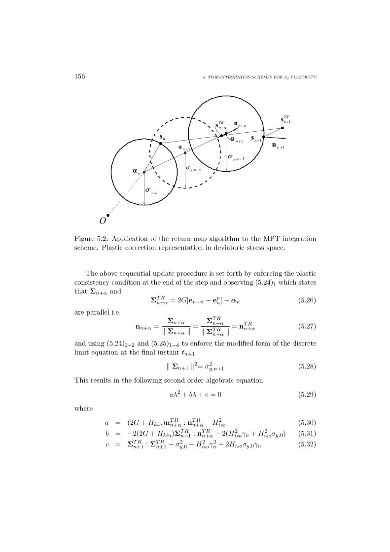
156 5. TIME-INTEGRATION SCHEMES FOR J2 PLASTICITY
n
,y n
, 1y n
,y n
n
1n
1nn
1
TR
ns
1nsns
O
TR
ns nn
Figure 5.2: Application of the return map algorithm to the MPT integrationscheme. Plastic correction representation in deviatoric stress space.
The above sequential update procedure is set forth by enforcing the plasticconsistency condition at the end of the step and observing (5.24)1 which statesthat Σn+α and
ΣTRn+α = 2G[en+α − ep
n]−αn (5.26)
are parallel i.e.
nn+α =Σn+α
‖ Σn+α ‖=
ΣTRn+α
‖ ΣTRn+α ‖
= nTRn+α (5.27)
and using (5.24)1−2 and (5.25)1−4 to enforce the modified form of the discretelimit equation at the final instant tn+1
‖ Σn+1 ‖2= σ2y,n+1 (5.28)
This results in the following second order algebraic equation
aλ2 + bλ+ c = 0 (5.29)
where
a = (2G+Hkin)nTRn+α : nTR
n+α −H2iso (5.30)
b = −2(2G+Hkin)ΣTRn+1 : nTR
n+α − 2(H2isoγn +H2
isoσy,0) (5.31)c = ΣTR
n+1 : ΣTRn+1 − σ2
y,0 −H2isoγ
2n − 2Hisoσy,0γn (5.32)

5.4. GENERALIZED MIDPOINT INTEGRATION SCHEME FOR THE LP MODEL 157
It is assumed that the plastic rate parameter λ which permits the updates(5.24) and (5.25) is given by the minimum positive root.
5.4.3 MPT scheme elastoplastic consistent tangent operator
The elastoplastic consistent tangent operator at tn+1 follows at once by a chainrule argument, once it is derived at tn+α. The reader can refer to [7, 13, 17, 72]for a detailed derivation of this part. For brevity’s sake, we just report the finalform of the operator for a plastic step (i.e. such that λ = 0) without derivingit thoroughly. To make notation more clear, the subscripts of all variables areomitted and it is implicitly assumed that all quantities are evaluated at thefinal instant of the step tn+1. Recalling that
∂s∂ε
=∂s∂e
∂e∂ε
=∂s∂e
Idev (5.33)
where
Idev = I− 13
(I⊗ I) (5.34)
and taking into account the volumetric part of the stress, from Equations (5.1),(5.2) and (5.3) we get
Cep =
∂σ
∂ε=∂s∂e
Idev +K (I⊗ I) (5.35)
The fourth-order tensor∂s∂ε
can be computed as
∂s∂e
= m1 + m2 (5.36)
where m1 and m2 are given by the following expressions
m1 = 2G(
I− β1
β1 + β2 + 1In − nn+α ⊗
∂λ
∂e
)(5.37)
m2 =β1
β1 + β2 + 1In
(β ⊗ ∂λ
∂e
)(5.38)

158 5. TIME-INTEGRATION SCHEMES FOR J2 PLASTICITY
with
In = I− nn+α ⊗ nn+α (5.39)∂λ
∂e= −2Gθ−1
1
(I− 2Gλ+Hkinλ/2
2 ‖ sTRn+α −αn ‖
In
)Σn+1 (5.40)
β =12Hkinnn+α (5.41)
θ1 = Hisoσy,n+1 + (β : Σn+1) + 2G (nn+α : Σn+1) (5.42)
β1 =2Gλ
2‖Σn+α‖(5.43)
β2 =Hkinλ
2‖Σn+α‖(5.44)
5.5 ENN exponential-based integration scheme forthe LP model
This section presents the first exponential-based integration algorithm for von-Mises plasticity with linear hardening, initially presented and implemented byAuricchio and Beirao da Veiga [16]. A similar idea had been developed byHong and Liu [44, 45]. This algorithm which is labeled ENN (Exponential-based Non-symmetric Non-consistent method) constitutes the first memberof the exponential-based family object of this work and is characterized bysecond-order accuracy, exactness in case of zero isotropic hardening, yet bynot being yield-consistent.
The integration scheme is based on a model reformulation by a rewritingof the constitutive equations and on the choice for an integration factor. Theresulting evolutive equation for a generalized stress tensor results of notableinterest since it is quasi-linear. Under suitable hypotheses the time integra-tion of the above quasi-linear dynamical system can be carried out with theexponential maps technique.
5.5.1 A new model formulation
Combining Equations (5.4) and (5.5), we obtain
Σ + α + 2Gep = 2Ge (5.45)
and, taking the derivative in time and applying Equation (5.9), Equation (5.45)becomes
Σ + (2G+Hkin) ep = 2Ge (5.46)

5.5. ENN EXPONENTIAL-BASED INTEGRATION SCHEME FOR THE LP MODEL 159
Now, recalling that in the plastic phase
n =Σ‖ Σ ‖ =
Σσy,0 +Hisoγ
(5.47)
we may apply (5.7) obtaining
Σ + (2G+Hkin)Σ
σy,0 +Hisoγγ = 2Ge (5.48)
which is a differential equation for Σ. We now need an evolution law for γ,which in the elastic phase is simply
γ = 0 (5.49)
while in the plastic phase it is indirectly extracted from the Kuhn-Tuckercondition F = 0. Multiplying Equation (5.48) by Σ it follows
Σ : Σ + (2G+Hkin)‖ Σ ‖2
σy,0 +Hisoγγ = 2G [e : Σ] (5.50)
and, observing that in the plastic phase
‖ Σ ‖2 = (σy,0 +Hisoγ)2 (5.51)
Σ : Σ =12
ddt‖ Σ ‖2= Hiso (σy,0 +Hisoγ) γ (5.52)
it becomes
(σy,0 +Hisoγ) (2G+Hkin +Hiso) γ = 2G [e : Σ] (5.53)
Now the idea is to rewrite the differential system formed by equations (5.48)and (5.49)-(5.53) introducing an integrating function. Accordingly, we set
X0(γ) =
(1 +
Hiso
σy,0γ
)2G+Hkin
Hisoif Hiso = 0
exp
(2G+Hkin
σy,0γ
)if Hiso = 0
(5.54)
noting that such a function is continuous for fixed γ andHiso → 0. MultiplyingEquation (5.48) by X0(γ), we have
ddt
[ΣX0(γ)] = 2GeX0(γ) (5.55)

160 5. TIME-INTEGRATION SCHEMES FOR J2 PLASTICITY
At this stage, we define a new generalized stress vector X which, adopting theengineering notation reads
X =X0ΣX0
=Xs
X0
(5.56)
from (5.55) we obtainX
s= 2GX0e (5.57)
We now search a similar differential equation for the last component X0 of X.Taking the derivative of X0(γ), we have
X0 =ddtX0(γ (t)) = (2G+Hkin)
X0
σy,0 +Hisoγγ (5.58)
From (5.58) and (5.53) we obtain
X0 =2G+Hkin
σ2y,0 (2G+Hkin +Hiso)
X0(1 +
Hiso
σy,0γ
)2 [2Ge : Σ] =
=2G+Hkin
σ2y,0 (2G+Hkin +Hiso)
X−
2Hiso
2G +Hkin0 [2Ge : Xs] (5.59)
Introducing the position
χ = χ(X0) =2G+Hkin
σ2y,0 (2G +Hkin +Hiso)
X−
2Hiso
2G+Hkin0 (5.60)
and, recalling Equation (5.49), we have
X0 = 0 (elastic phase) (5.61)
X0 = 2G χ e : Xs (plastic phase) (5.62)
We introduce now a linear space structure on the space of generalized stresseswhich is the key feature of the exponential-based formulation. Any element ofthe space of linear operators from the generalized stress space into itself canbe written adopting the engineering notation as
[M] =[
M11 M12
M21 M22
](5.63)

5.5. ENN EXPONENTIAL-BASED INTEGRATION SCHEME FOR THE LP MODEL 161
with M11 a fourth-order tensor, M12,M21 second-order tensors and M22 ascalar, under the convention that the formal expression
MY (5.64)
returns a generalized stress vector given by the following operation
[M] Y =[
M11 M12
M21 M22
]Ys
Y0
=
M11Ys + M12Y 0
M21 : Ys + M22Y0
(5.65)
for any couple Y = Ys, Y0T in the generalized stress space. The productby a scalar and the sum between vectors is defined in the obvious naturalway. Accordingly, Equations (5.57) and (5.61)-(5.62) provide a system for thegeneralized stress vector X
X = AX (5.66)
with the matrix operator A depending on the actual phase
[A] = [Ae] = 2G[O e0 0
](elastic phase) (5.67)
[A] = [Ap] = 2G[
O eχe 0
](plastic phase) (5.68)
where 0 and O indicate respectively the second-order and fourth-order null ten-sors. Therefore, the original problem, represented by Equations (5.3)-(5.10),is replaced by a new one, where the relative stress Σ and the plastic rate γare now represented in the form of vector X. The main advantage of the newform is the quasi-linearity, both in the elastic and in the plastic phase.
As an example, let us consider the model with no isotropic hardening(Hiso = 0). Due to Equations (5.60) and (5.68), it is immediate to checkthat A depends only on e. This means that, if e is constant in a certain timeinterval, A holds the same property: under such a hypothesis the solution ofsystem (5.66) is known and the problem can be solved exactly.
However, in the general case, the matrix A depends on X, and in this sensewe say that the problem is quasi-linear. Anyway, the partial linearity arisingin the problem is indeed of great value, allowing us to numerically approximateits solution with excellent results.
Time-continuous on-off switch
To properly convert the original problem in an equivalent but new differentialalgebraic format, we also need to introduce an elastic-plastic phase determi-nation criteria expressed in the new generalized stress environment.

162 5. TIME-INTEGRATION SCHEMES FOR J2 PLASTICITY
For a given phase to be plastic, the following two conditions hold:
1) The relative stress Σ must be on the yield surface
‖ Xs ‖2=‖ Σ ‖2 X20 = (σy,0 +Hisoγ)
2X20 = σ2
y,0X
2(Hiso +Hkin + 2G)2G +Hkin
0
(5.69)
2) The direction of the strain rate e must be outward with respect to theyield surface
Σ : e > 0 ⇐⇒ Xs : e > 0 (5.70)
If such two conditions are not satisfied, the step is elastic.
5.5.2 Integration scheme
In the following we present a numerical scheme for the evolution of X, gov-erned by the dynamical law (5.66) with matrix A given by (5.67) or (5.68)respectively.
As usual, we assume that the time history interval [0, T ] is divided into Nsub-intervals defined by the nodes 0 = t0 < t1 < .... < tn < tn+1 < .... < tN =T and indicate the general sub-interval amplitude as ∆t = tn+1 − tn. Giventhe values sn, en, e
pn, γn,αn at time tn and the deviatoric strain en+1 at time
tn+1, we search for the remaining variables at time tn+1, assuming the strainhistory to be piecewise linear. The strain is retained taken as a linear functionin each time sub interval and, for simplicity, we consider the initial values ofγ and α to be zero, so that the initial generalized stress vector is
X0 =Xs
0
X0
=Σ0
1
(5.71)
Clearly, the initial values of the relative stress and the deviatoric strain mustbe consistent with the governing Equations (5.3)-(5.10).
The evolution of X is governed by the dynamical law (5.66) with matrixA given by (5.67) or (5.68). Due to the piecewise linearity of the strain path,e is constant in each single time interval. Unluckily, due to the presence of χin (5.68), this is not true for matrix A; the scalar χ is a function of X0, and soof X, as shown in Equation (5.60). Therefore, we approximate the solution ofthe dynamical law (5.66) considering χ constant in each single time step. Thediscrete form of the evolution law (5.66) becomes
X = AX (5.72)

5.5. ENN EXPONENTIAL-BASED INTEGRATION SCHEME FOR THE LP MODEL 163
where the matrix A is now constant along a single time interval
[A]
= 2G[O e0 0
](elastic step) (5.73)
[A]
= 2G[
O eχne 0
](plastic step) (5.74)
Under such an additional hypothesis, the matrix A is constant in bothphases, and so the evolution of Equation (5.72) is well known to be
Xn+1 = exp[A∆t
]Xn (5.75)
where ∆t = tn+1−tn. Defining the tensor ∆e = en+1−en, we observe that thematrix A∆t is equal to the matrix (5.67) or (5.68) after substituting e with ∆e.Note that, being A an element in the linear space of linear operators actingon couples, the exponential of A∆t is naturally defined by the (converging)exponential serie
G = exp[A∆t
]=
+∞∑n=0
(A∆t
)nn!
(5.76)
The linear operator G appearing in Equation (5.75) can be derived calculatingthe shown exponential. Note that, for such purpose, it is convenient to refor-mulate the linear operator A∆t as a R7×7 matrix, calculate the exponential,and finally write it back in the original form (5.63).
Hence, given the initial value Xn, Xn+1 can be now calculated as
Xn+1 = G Xn (5.77)
The matrix G is the exponential appearing in (5.76), which is
[Ge
]=
I 2G∆e
0 1
(5.78)
for an the elastic step, and
[Gp
]=
I +
[(a− 1)
‖ ∆e ‖2
]∆e⊗∆e
b√χ
∆e‖ ∆e ‖
b√χ
∆e‖ ∆e ‖ a
(5.79)

164 5. TIME-INTEGRATION SCHEMES FOR J2 PLASTICITY
for a plastic step. The scalars a and b are
a = cosh (2G√χ ‖ ∆e ‖)
b = sinh (2G√χ ‖ ∆e ‖)
while χ is given by (5.60) calculated in X0n, i.e. the last component of Xn.
Such a choice of χ is not only natural (we take its value at the start of thestep) but also of simple application. More accurate and performing choicescould be introduced, perhaps requiring some implicit calculation instead of thedirect matrix product (5.77).
5.5.3 Solution algorithm
At every time step the numerical scheme is as follows:
1) suppose the step to be elastic and compute trial values following anelastic law
XTRn+1 = GeXn (5.80)
where the matrix Ge is given by (5.78). If the trail solution is admissible,i.e.
‖ XTRn+1 ‖≤ σy,0
(XTR
0,n+1
)Hiso +Hkin + 2G2G+Hkin (5.81)
then the history variables at the time step tn+1 are taken as the trialones just calculated.
2) If the trail solution is not admissible, i.e. Equation (5.81) is violated,then the step is plastic. Being e constant in each sub time interval, thismeans that the step can be divided into two parts: an elastic deformationfollowed by a plastic one. We represent with a scalar α ∈ [0, 1) theelastic time proportion of the step; for example α = 1/2 means that thestress evolution is of elastic kind for the first half of the time interval,and plastic in the rest. Simple geometrical considerations allow us tocompute α; without discussing the details, the obtained value is
α =√C2 −DM − C
D(5.82)
where
C = 2GX0,n (Xsn) : ∆e
D = (2GX0,n ‖ ∆e ‖)2
M =‖ Xsn ‖2 −σ2
y,0 (X0,n)2ϕ
ϕ =2G+Hkin +Hiso
2G+Hkin
(5.83)

5.5. ENN EXPONENTIAL-BASED INTEGRATION SCHEME FOR THE LP MODEL 165
Computed α, Xn+1 is updated in two steps.
– Calculate XTRn+1 following an elastic law
XTRn+1 = GeXn (5.84)
with Ge still given by (5.78), but where ∆e = α (en+1 − en) insteadof ∆e = (en+1 − en).
– Calculate Xn+1 evolving from the new initial data XTRn+1 following
a plastic law:Xn+1 = GpXTR
n+1 (5.85)
with Gp given by (5.78), where ∆e = (1−α) (en+1 − en) instead of∆e = (en+1 − en).Observe that in such a framework purely plastic steps are simplythose where the time proportion of elastic phase α is zero.
3) Whenever needed, calculate the relative stress and backstress as:
Σ =Xs
X0(5.86)
α = Hkinep = Hkin2Ge−Σ
2G +Hkin(5.87)
The first one is immediately obtained from the definition of X, while thesecond one follows from (5.4) and (5.5), observing that α = Hkinep.
4) Finally, at the end of each step, update the constant χ = χ(X0,n+1) usedfor the calculation of the matrix Gp.
Remark 3: Due to the approximation introduced assuming χ constant ineach time step, during a plastic step Equation (5.69) is not exactly enforced(while in the BE method this is fulfilled). However, this discrepancy seems toresolve in very small numerical errors as shown in the examples that follow.A cure to this could be a radial projection of the solution on the yield surfaceat the end of each time step: this idea indeed leads to the development of thenext algorithm (ENC algorithm). Nevertheless, it is observed that introducingsuch a correction does not change significantly the solution. In Section 5.7 twoalgorithms improved to be yield-consistent with no need of a radial projectionat the end of plastic steps are presented.

166 5. TIME-INTEGRATION SCHEMES FOR J2 PLASTICITY
5.5.4 ENN scheme elastoplastic consistent tangent operator
The algorithmically consistent tangent operator can be obtained properly lin-earizing the time-discrete procedure. To make notation more clear, the sub-scripts of all history variables evaluated at time tn+1 are omitted for brevity.Quantities evaluated at tn are specified by the relative subscript.
From the definition of the generalized stress tensor X we get
∂Xs
∂e= Σ⊗ ∂X0
∂e+X0
∂Σ∂e
(5.88)
hence∂Σ∂e
=1X0
(∂Xs
∂e−Σ⊗ ∂X0
∂e
)(5.89)
For the elastic phase we immediately have
∂Xs
∂e= 2GX0I (5.90)
∂X0
∂e= 0 (5.91)
while in the plastic phase the result is slightly more complicated and can befound in the sequel.For the deviatoric stress, Equation (5.5) provides
∂s∂e
=∂Σ∂e
+∂α
∂e(5.92)
and, recalling also Equation (5.87), it becomes
∂s∂e
=2G
2G+Hkin
∂Σ∂e
+2GHkin
2G+HkinI (5.93)
We also have∂s∂ε
=∂s∂e
∂e∂ε
=∂s∂e
Idev (5.94)
Taking into account the volumetric part of the stress, from Equations (5.1),(5.2) and (5.3), we obtain the tangent operator
Cep =
∂σ
∂ε=∂s∂ε
+K (I⊗ I) (5.95)
Joining statements (5.89), (5.93), (5.94) and (5.95) we obtain
∂σ
∂ε=
2GX0(2G +Hkin)
(∂Xs
∂e−Σ
∂X0
∂e
)Idev +
2GHkin
2G+HkinIdev +K (I⊗ I)
(5.96)

5.5. ENN EXPONENTIAL-BASED INTEGRATION SCHEME FOR THE LP MODEL 167
which in the elastic case simplifies to the usual
∂σ
∂ε= 2GIdev +K (I⊗ I) (5.97)
and in the plastic one can be calculated substituting the fourth-order tensor∂Xs/∂e and the second-order tensor ∂X0/∂e, which can be deduced as follows.The fourth-order tangent tensor ∂Xs/∂e and the second-order tangent tensor∂X0/∂e provide the tangent operator ∂σ/∂ε of the new algorithm duringplastic or mixed elastoplastic steps (cf. Equation (5.96)). Remembering thatpurely plastic steps are a particular case within the range of mixed ones (seeSection 5.5.3), we start analyzing the latter. We have, from (5.84)-(5.85),
Xn+1 = GpGeXn = Gp((1 − α)∆e) Ge(α∆e) Xn (5.98)
where the tensors above are given by (5.78)-(5.79) and α = α(∆e) is the “elas-tic step proportion” defined in (5.82). Consequently, following basic derivationrules, we have for mixed steps
∂Xn+1
∂e=[A1 + A2 + A3 + A4
]Xn (5.99)
where the matrix operators
A1 =∂Gp
∂∆e[(1− α)∆e] Ge(α∆e)
A2 =∂Gp
∂α[(1− α)∆e]
dαd∆e
(∆e) Ge(α∆e)
A3 = Gp[(1− α)∆e]∂Ge
∂∆e(α∆e)
A4 = Gp[(1− α)∆e]∂Ge
∂ α(α∆e)
dαd∆e
(∆e)
(5.100)
From Equation (5.99) we can derive ∂Xsn+1/∂e and ∂X0,n+1/∂e; in order to
obtain the classical tangent operator, the obtained equations must be finallyexpressed as a linear function of the strain of the form (5.99), which is expressedas a linear function of Xn. Doing so, we finally obtain that for mixed steps
∂Xs
∂e= (A1 + A2 + A3 + A4) (5.101)
∂X0
∂e= (b1 + b2 + b3 + b4) (5.102)
where the fourth-order tensors A and the second-order tensors b are describedbelow without addressing the calculations.

168 5. TIME-INTEGRATION SCHEMES FOR J2 PLASTICITY
For purely plastic steps, being α constantly equal to zero, we obtain the shorterformulation
∂Xs
∂e= A1 (5.103)
∂X0
∂e= b1 (5.104)
We start introducing (cf. (5.82) for M,D,C in each step) the υ = dα/d∆esecond-order tensor
υ = φ1dCd∆e
+ φ2dDd∆e
φ1 =1D
(C√
C2 −DM− 1)
φ2 = − 1D2
(DM
2√C2 −DM
+√C2 −DM − C
)dCd∆e
= 2GX0,n Xsn
dDd∆e
= 2(2GX0,n)2∆e
(5.105)
Let the scalars
a = cosh (2G(1 − α)√χ ‖ ∆e ‖)
b = sinh (2G(1 − α)√χ ‖ ∆e ‖)
s =∆e : Xs
n
‖ ∆e ‖k = 2G(1 − α)
√χ
k = −2G√χ ‖ ∆e ‖
(5.106)
and the operators
M1 = s
(kb− 2
a− 1‖ ∆e ‖
)[∆e⊗∆e
‖ ∆e ‖2]
+(a− 1)s‖ ∆e ‖ I +
a− 1‖ ∆e ‖
[∆e⊗Xs
n
‖ ∆e ‖
] (5.107)
M2 =(ka− b
‖ ∆e ‖
)[∆e⊗∆e
‖ ∆e ‖2]
+b
‖ ∆e ‖I (5.108)

5.6. ENC EXPONENTIAL-BASED INTEGRATION SCHEME FOR THE LP MODEL 169
We then have, for the tensors in (5.101),
A1 = M1 +X0,n√χ
M2
A2 = k
(bs+
a√χX0,n
)[∆e⊗ υ
‖ ∆e ‖
]A3 = 2GαX0,n
[I + (a− 1)
∆e⊗∆e
‖ ∆e ‖2]
A4 = 2GaX0,n [ ∆e⊗ υ] ;
(5.109)
and for the tensors appearing in (5.102)
b1 =√χ M2Xs
n + kbX0,n∆e‖ ∆e ‖
b2 = k (as√χ+ bX0,n) υ
b3 = 2GαbX0,n√χ
∆e‖ ∆e ‖
b4 = 2GbX0,n√χ ‖ ∆e ‖ υ
(5.110)
5.6 ENC exponential-based integration scheme for
the LP model
5.6.1 ENC scheme: an enforced consistency variant of theENN scheme
As it is shown by the numerical tests carried out in the next chapter, whencompared to the BE scheme and to the ESC algorithm which will be addressedin the next section, the ENN scheme shows far better precision propertiesand second-order accuracy. On the other hand, as already observed in [16],the ENN algorithm presented above is not consistent with the yield surfacecondition. In other words, at the end of plastic steps, condition (5.69) doesnot hold exactly for the numerical solution.
Apart from physical considerations, the above property is important alsofor the stability of the algorithm; whenever the numerical relative stress Σ fallsout of the yield surface (i.e. ‖ Σn+1 ‖> σy,n+1) this may lead to instabilitiesin the following time step. Therefore, in practical applications, it is recom-mendable to enforce the consistency at the end of each elastoplastic step. Thiscan be achieved using a radial projection of the relative stress onto the yieldsurface in each time step in which ‖ Σn+1 ‖> σy,n+1 by simply multiplyingΣn+1 by the rate σy,n+1/ ‖ Σn+1 ‖).

170 5. TIME-INTEGRATION SCHEMES FOR J2 PLASTICITY
The ENC yield-consistent variant of the ENN scheme is implemented fol-lowing this idea. The consistency check can be done either at the start ofeach step or at the end. It is to be pointed out that the algorithmical stepsof this methods remain the same as the ones described in the previous sectionwith respect to the ENN method. In particular, the enforced consistency vari-ant ENC allows to use the same algorithmic consistent elastoplastic tangentoperator calculated for the ENN scheme.
5.7 ESC-ESC2 exponential-based integration sche-
mes for the LP model
5.7.1 An innovative model formulation
In this section we present a new time-continuous model formulation for thedifferential algebraic problem under consideration [9, 10, 11]. This innova-tive statement of the problem represents a generalisation of the formulationspresented in [6, 8] and thus constitutes an extension of the ones proposed in[44, 45, 16]. Such a formulation still allows to rewrite the system in the form
X = AX (5.111)
which is the starting point for the numerical scheme developed in Section5.7.2. As it will be cleared and substantiated on mathematical grounds by thetheoretical analysis carried out in the next Section 5.8, one of the algorithmsstemming from the present reformulation (ESC2 algorithm) shows to be the“optimal” one within the exponential-based integration algorithms class forthe LP elastoplastic model.
Combining Equations (5.4) and (5.5), we obtain
Σ + α + 2Gep = 2Ge (5.112)
which, taking the derivative in time, applying Equation (5.9) and rearrangingterms gives
Σ = 2Ge− (2G+Hkin) ep (5.113)
Now, recalling the yield surface radius
σy = σy,0 +Hisoγ (5.114)
and that in the plastic phase
n =Σ‖Σ‖ =
Σσy,0 +Hisoγ
=Σσy
(5.115)

5.7. ESC-ESC2 EXPONENTIAL-BASED INTEGRATION SCHEMES FOR THE LP MODEL 171
we may apply (5.7) obtaining
Σ + (2G+Hkin)Σσyγ = 2Ge (5.116)
which is a differential equation for Σ that is valid also during elastic phases(γ = 0). Introducing the scaled relative stress
Σ =Σσy
(5.117)
we observe that, whenever the relative stress Σ lays on the yield surface, thenΣ = n, while this is not true when Σ lays inside the yield surface. The timederivative of (5.117) and the use of relation (5.114) gives
˙Σ =Σσy− Hiso
σyγΣ (5.118)
Dividing Equation (5.116) by σy and using relationship (5.118), one obtains
˙Σ +2G+Hkin +Hiso
σyγΣ =
2Gσy
e (5.119)
The next goal is to introduce an integration factor for the above evolutionaryequation. Accordingly, we set
X0(γ) =
(1 +
γHiso
σy,0
)2G+Hkin +Hiso
Hisoif Hiso = 0
exp
(2G +Hkin +Hiso
σy,0γ
)if Hiso = 0
(5.120)
noting that such a function is continuous for fixed γ and Hiso → 0 and that
X0 =2G+Hkin +Hiso
σyγX0 (5.121)
Multiplying Equation (5.119) by X0 and using equation (5.121) the followingrelationship holds
ddt[X0Σ
]= X0
˙Σ + X0Σ =2GσyX0e (5.122)

172 5. TIME-INTEGRATION SCHEMES FOR J2 PLASTICITY
At this stage, defining the generalized stress vector X as
X =X0ΣX0
=Xs
X0
(5.123)
Equation (5.122) can be rewritten as
Xs
=2GσyX0e (5.124)
The evolution law for X0 in terms of X in elastic phases follows immediatelyfrom (5.121):
X0 = 0 (elastic phases) (5.125)
On the other hand, for γ = 0, taking the scalar product of (5.122) with Σ, wehave
X012
ddt‖Σ‖2 + X0‖Σ‖2 =
2GσyX0e : Σ (5.126)
which, noting that in plastic phases
‖Σ‖ =‖Σ‖σy
= 1 (5.127)
and using (5.123), (5.126) gives
X0 =2Gσy
e : Xs (plastic phases) (5.128)
Equations (5.124), (5.125) and (5.128) provide a system for the generalizedstress vector X, in the form
X = AX (5.129)
with the matrix A depending on the actual phase as follows
[A] = [Ae] =2Gσy
[O eO 0
](elastic phase) (5.130)
[A] = [Ap] =2Gσy
[O ee 0
](plastic phase) (5.131)
where 0 and O indicate respectively the second-order and fourth-order ordernull tensors. In the last statement, Equation (5.129), we have made use of thelinear operator space structure introduced in the previous section (cf. Equa-tions (5.63)-(5.65). Note that A is symmetric during plastic phases. Therefore

5.7. ESC-ESC2 EXPONENTIAL-BASED INTEGRATION SCHEMES FOR THE LP MODEL 173
the original problem, expressed by Equations (5.4)-(5.9), has been substitutedby a new one, expressed by Equations (5.129)-(5.131).
We also observe that in the case of no isotropic hardening (Hiso = 0) theyield radius σy is fixed and therefore A depends only on e. This means that, ife is constant in a given time interval, A holds the same property: under suchan hypothesis the solution of system (5.129) is known and the problem can besolved exactly.
However, in a general case (Hiso = 0) the matrix A depends on X and inthis sense we say that the problem is quasi-linear. Anyway, the quasi-linearityarising in the problem is indeed of great value, allowing us to develop thenumerical method of Section 5.7.2.
Time-continuous on-off switch
To properly convert the original problem in a new but equivalent differentialalgebraic format, we also need to introduce an elastoplastic phase determina-tion criterium expressed in the new generalized stress environment.
For a given state to be plastic, the following two conditions must be fulfilled:
1) The relative stress Σ must be on the yield surface, in other words
‖Σ‖ = σy (5.132)
Using (5.117) and (5.123) this can be easily rewritten as
‖Xs‖2 = ‖Σ‖2X20 =‖Σ‖2σ2
y
X20 = X2
0 (5.133)
2) The direction of the strain rate e must be outward with respect to theyield surface, i.e.
Σ : e > 0 (5.134)
Again, recalling (5.117) and (5.123) it is immediate to check that (5.134)is equivalent to
Xs : e > 0 (5.135)
If the two conditions (5.133) and (5.135) are not satisfied, the step is elastic.
5.7.2 Integration scheme
We now want to develop a numerical scheme for the evolution of X, gov-erned by the dynamical law (5.129) with matrix A given by (5.130) or (5.131)respectively.

174 5. TIME-INTEGRATION SCHEMES FOR J2 PLASTICITY
As usual, we assume that the time history interval [0, T ] is divided into Nsub-intervals defined by the nodes 0 = t0 < t1 < .... < tn < tn+1 < .... < tN =T and indicate the general sub-interval amplitude as ∆t = tn+1 − tn. Giventhe values sn, en, e
pn, γn,αn at time tn and the deviatoric strain en+1 at time
tn+1, we search for the remaining variables at time tn+1, assuming the strainhistory to be piecewise linear. For simplicity, we consider the initial values (att = t0) of γ, ep and α to be zero, so that the initial generalized stress vector is
X0 =Σ0/σy,0
1
(5.136)
Due to the piecewise linearity of the strain path, e is constant in each singletime interval. Unluckily, due to the presence of σy in (5.131), during plasticphases, the matrix A is not constant in the same time interval; in fact the yieldsurface radius σy is a function of X0, as shown by relation (5.121) and henceof X. Therefore, we discretize the dynamical law (5.129), approximating σy
stepwise. Along each time interval [tn, tn+1], we choose σy = R, where R isnow a constant value in each single time step. It is evident that for purelyelastic steps R coincides with σy,n. The discrete form of the evolution law(5.129) becomes
X = AX (5.137)
where the matrix A is now constant along a single time interval[A]
=2Gσy,n
[O e0 0
](elastic step) (5.138)
[A]
=2GR
[O ee 0
](plastic step) (5.139)
Different choices for R are possible [11], for exampleR = σy,n (ESC scheme)
R =cσy,n
ln(1 + c)(ESC2 scheme)
(5.140)
where
c =
2G q (1− α)
(Xs
n
X0,n: e
)σy,n
∆t (5.141)
withq =
Hiso
2G+Hkin +Hiso(5.142)

5.7. ESC-ESC2 EXPONENTIAL-BASED INTEGRATION SCHEMES FOR THE LP MODEL 175
The α scalar parameter represents the part of the step along which the stressremains within the limit surface (see Figure 5.3). Its calculation will be ex-plained and discussed in detail in Section 5.7.3 for compactness reasons.
The first choice for R in (5.140) corresponds to the ESC scheme proposedin [8], the second one leads to the new ESC2 scheme [11]. While the rea-sonings for the first choice for R are evident (“forward integration” scheme),the second choice for R comes from considerations regarding the improvednumerical properties of the new exponential-based algorithm, discussed fromthe analytical standpoint in Section 5.8.
Due to the fact that R is computed using only quantities evaluated at thebeginning of the step, the matrix A is now constant in both elastic and plasticphases and so Equation (5.137) can be solved exactly, giving the followingevolution for X
Xn+1 = exp[A∆t
]Xn = G Xn (5.143)
Note that, being A an element in the linear space of linear operators actingon couples, the exponential of A∆t is naturally defined by the (converging)exponential serie
G = exp[A∆t
]=
+∞∑n=0
(A∆t
)nn!
(5.144)
Defining the tensor ∆e = en+1 − en, we observe that the matrix A∆t isequal to the matrix (5.138) or (5.139) after substituting e with ∆e. The linearoperator G can be derived calculating the shown exponential. Note that, forsuch purpose, it is convenient to reformulate the linear operator A∆t as aR7×7
matrix, calculate the exponential, and finally write it back in the original form(5.63). Without showing the calculations, one finds
[G]
=
[Ge
]=
I2Gσy,n
∆e
O 1
(elastic phase)
[Gp
]=
I +[(a− 1)‖∆e‖2
]∆e⊗∆e b
∆e‖∆e‖
b∆e‖∆e‖ a
(plastic phase)
(5.145)

176 5. TIME-INTEGRATION SCHEMES FOR J2 PLASTICITY
where the scalars a and b are
a = cosh(
2GR‖∆e‖
)(5.146)
b = sinh(
2GR‖∆e‖
)(5.147)
5.7.3 Solution algorithm
At every time step the exponential-based algorithm proceeds as follows:
1) suppose the step to be elastic and compute trial values following anelastic law
XTRn+1 = GeXn (5.148)
where the matrix Ge is given by (5.145). If the trial solution is admissible,i.e.
‖Xs,TRn+1 ‖ ≤
(XTR
0,n+1
)2(5.149)
then the history variables at the time step tn+1 are taken as the trialones just calculated.
2) If the trial solution is not admissible, i.e. Equation (5.149) is violated,then the step is plastic or elastoplastic. Being e constant in each time subinterval, the step can be divided into two parts: an elastic deformationtaking place during [tn, tn+α], followed by a plastic one along [tn+α, tn+1].Hence, we represent with a scalar α ∈ [0, 1) the elastic time proportionof the step. The key consideration in order to calculate α is that theevolution during the partial elastic sub-step is linear in stress space.Accordingly, recalling (5.145), we search for an intermediate generalizedstress vector
Xs,en+1 = Xs
n +2GX0,n
σy,n[α∆e] (5.150)
such that Xs,en+1 represents a relative stress tensor lying on the yield
surface at time tn+α. In other words, we must request
Xs,en+1 : Xs,e
n+1 −X20,n = 0 (5.151)
Note that the left hand side of the above equation is a second orderpolynomial in α. In stress space, the roots of such polynomial correspondto the intersections between a segment and the boundary of a sphere,where an extreme of the segment (sn) lays inside the sphere closure andthe other extreme (sn + 2G∆e) outside the sphere. As a consequence,

5.7. ESC-ESC2 EXPONENTIAL-BASED INTEGRATION SCHEMES FOR THE LP MODEL 177
there is always one maximum (non-negative) root. Calculating thereforeα from expression (5.151) we get
α =
√C2 −DM − C
D(5.152)
where
C =2GX0,n
σy,n(Xs
n : ∆e)
D =(
2GX0,n‖∆e‖σy,n
)2
M = ‖Xsn‖2 −
(XTR
0,n+1
)2(5.153)
Computed α, Xn+1 is updated in two steps.
– Calculate a new Xen+1 vector following an elastic law along an α∆t
intervalXe
n+1 = Ge[α∆e]Xn (5.154)
– Calculate Xn+1 evolving from the new initial data Xen+1 following
a plastic law along the remaining part of the interval of amplitude(1− α)∆t
Xn+1 = Gp[(1− α)∆e]Xen+1 (5.155)
Observe that in such a framework purely plastic steps are simplythose where the time proportion of the elastic phase α is zero.
3) Update the yield surface radius
σy,n+1 = σy(X0,n+1) = σy,0 (X0,n+1)q (5.156)
which is easily obtained combining (5.114) and (5.120).
The updating procedure illustrated by steps 1) - 3) is represented in Figure5.3 which refers to the space of tensors Xs.
Remark 5.7.1 The relative stress and backstress can be calculated wheneverneeded as:
Σ =Xs
X0σy (5.157)
α = Hkin2Ge−Σ
2G+Hkin(5.158)
The first one is immediately obtained from the definition of X, while the secondone follows from (5.4) and (5.5), observing that α = Hkinep.

178 5. TIME-INTEGRATION SCHEMES FOR J2 PLASTICITY
Figure 5.3: Updating procedure in generalized stress space for the ESC andESC2 scheme during a mixed elastoplastic step.
Remark 5.7.2 The variableX0 is a local auxiliary variable and not an historyvariable. In other words, introducing an appropriate scaling of the vector Xthe variable X0 does not need to be updated at every time step [8].
Remark 5.7.3 Whenever Hiso = 0, i.e. there is no isotropic hardening, thesolution obtained with this scheme is exact. Other exact integrators can befound in the literature for the case Hiso = 0 [51, 67, 77]. A discussion ofexponential-based exact integration schemes and other exact integrators canbe found in [8].
5.7.4 ESC2 scheme elastoplastic consistent tangent operator
In the following we present the tangent operator of the new optimal exponential-based ESC2 integration scheme. For what concerns the ESC scheme, thereader is referred to [8] where a complete derivation of its tangent operatoris developed. As it will be clear in the following, the tangent moduli opera-tor corresponding to the ESC algorithm can be obtained in a straightforwardmanner by simply canceling the A5 and e5 terms arising in the new discreteformulation. To make notation more clear, the subscripts of all history vari-ables evaluated at time tn+1 are omitted for brevity. Quantities evaluatedeither at tn or at tn+α are specified by the relative subscript.
We now present the tangent fourth-order tensor ∂Xs/∂e and the tangentsecond-order tensor ∂X0/∂e for plastic phases, which provide the elastoplastic
consistent tangent operator Cep =
∂σ
∂εof the new algorithm during plastic or

5.7. ESC-ESC2 EXPONENTIAL-BASED INTEGRATION SCHEMES FOR THE LP MODEL 179
mixed elastoplastic steps.Recalling that purely plastic steps are a particular case within the range
of mixed ones (see Section 5.7.2), we start analyzing the latter. From (5.154)-(5.155), we have
Xn+1 = GpGeXn = Gp[(1− α)∆e, R] Ge[α∆e] Xn (5.159)
where the above matrix operators are given by (5.145) and α (which depends on∆e) is the “elastic step proportion” defined in (5.152). Consequently, followingbasic differentiation rules, we have
∂Xn+1
∂∆e=[A1 + A2 + A3 + A4 + A5
]Xn (5.160)
with
A1 =∂Gp
∂∆e[(1 − α)∆e, R] Ge[α∆e]
A2 =∂Gp
∂α[(1− α)∆e, R]
dαd∆e
[∆e] Ge[α∆e]
A3 = Gp[(1− α)∆e, R]∂Ge
∂∆e[α∆e]
A4 = Gp[(1− α)∆e, R]∂Ge
∂ α[α∆e]
dαd∆e
[∆e]
A5 =∂Gp
∂R[(1− α)∆e, R]
∂R
∂∆e[∆e, σy,n] Ge[α∆e]
(5.161)
From Equation (5.160) we derive ∂Xsn+1/∂e and ∂X0,n+1/∂e; in order to ob-
tain the classical tangent operator, the obtained equations must be finallyexpressed as a linear function of the strain tensor instead of the form (5.160),which is expressed as a linear function of Xn. Doing so, we finally obtain thatfor mixed steps
∂Xs
∂e= A1 + A2 + A3 + A4 + A5 (5.162)
∂X0
∂e= b1 + b2 + b3 + b4 + b5 (5.163)
where the fourth-order tensors A and the second-order tensors b are describedbelow without addressing the calculations.For purely plastic steps, being α constantly equal to zero, we obtain the shorterformulation
∂Xs
∂e= A1 (5.164)
∂X0
∂e= b1 (5.165)
180 5. TIME-INTEGRATION SCHEMES FOR J2 PLASTICITY
We start introducing (see again (5.152) for M,D,C in each step) the second-order tensor υ = dα/d∆e
υ = φ1dCd∆e
+ φ2dDd∆e
φ1 =1D
(C√
C2 −DM− 1)
φ2 = − 1D2
(DM
2√C2 −DM
+√C2 −DM − C
)dCd∆e
=2Gσy,n
X0,n Xsn
dDd∆e
= 2(2Gσy,n
X0,n)2∆e
(5.166)
and the second-order tensor w
w = p (w1 + w2)
p =−σy,n
[c−1 ln(1 + c)]2
[1
c(1 + c)− ln(1 + c)
c2
]p1 =
2Gqσy,n
(∆e : Xsn)
p2 =(
2Gσy,n
)2
q(1− α)‖∆e‖2
w1 = (1− α)2Gqσy,n
Xsn − p1υ
w2 = p2υ +(
2Gσy,n
)2
q(1− α)∆e
(5.167)
Introducing the scalars
a = cosh(
2GR
(1− α)‖∆e‖)
b = sinh(
2GR
(1− α)‖∆e‖)
s =∆e : Xs
n
‖∆e‖
k =2GR
(1− α)
k = −2GR‖∆e‖
(5.168)

5.8. THEORETICAL ANALYSIS OF ALGORITHMICAL PROPERTIES OF THE ESC AND ESC2 SCHEMES 181
and the fourth-order tensors
M1 = s
(kb− 2
a− 1‖ ∆e ‖
)[∆e⊗∆e
‖ ∆e ‖2]
+(a− 1)s‖ ∆e ‖ I +
a− 1‖ ∆e ‖
[∆e⊗Xs
n
‖ ∆e ‖
] (5.169)
M2 =(ka− b
‖ ∆e ‖
)[∆e⊗∆e
‖ ∆e ‖2]
+b
‖ ∆e ‖I (5.170)
We can show that the tensors appearing in (5.162) are
A1 = M1 +X0,n M2
A2 = k (bs+ aX0,n)[∆e⊗ υ
‖ ∆e ‖
]A3 =
2GRαX0,n
[I + (a− 1)
∆e⊗∆e
‖ ∆e ‖2]
A4 =2GRaX0,n [ ∆e⊗ υ]
A5 = − kR
(bs
‖∆e‖2 + a
)[ ∆e⊗w]
(5.171)
while the second-order tensors in (5.163) are
b1 = M2Xsn + kbX0,n
∆e‖ ∆e ‖
b2 = k (as+ bX0,n) υ
b3 =2GRαbX0,n
∆e‖ ∆e ‖
b4 =2GRbX0,n ‖ ∆e ‖ υ
b5 = − kR
(as
‖∆e‖ + b‖∆e‖)
w
(5.172)
5.8 Theoretical analysis of algorithmical properties
of the ESC and ESC2 schemes
In this section we address from a theoretical point of view the following al-gorithmical properties for the ESC and ESC2 methods: yield consistency, ex-actness under proportional loading, accuracy and convergence. In particular

182 5. TIME-INTEGRATION SCHEMES FOR J2 PLASTICITY
we prove that the ESC scheme is yield consistent and converging with linearrate to the exact solution. The ESC2 scheme is yield consistent, exact in thecase of proportional loading and quadratically accurate. Moreover, limitingthe proof to purely plastic load histories, we show that the ESC2 scheme isquadratically convergent. Although purely plastic loadings are not uncommonin practical cases, a more complete approach should deal with generic loadinghistories; hence, this point is worth further investigation.
Finally, both schemes are exact in the case of materials with no isotropichardening. Note that the word “exact” means that the algorithm introducesno error for strain driven load histories under the classical hypothesis e piece-wise constant. In practical applications this does not translate directly intoexactness of the constitutive solver. This point will be cleared by the numericaltests and it will be briefly discussed in the following sections.
For basic results and definitions regarding the numerical integration ofordinary differential equations we refer for example to [39, 52].
5.8.1 Yield consistency
In the framework of the new formulation, recalling (5.117) and (5.123), theyield consistency condition
‖Σn+1‖ = σy,n+1 at end of each plastic step (5.173)
becomes
‖Xsn+1‖2 −X2
0,n+1 = 0 at end of each plastic step (5.174)
Both the ESC and ESC2 schemes are yield consistent, in other words satisfycondition (5.174). The proof for the ESC2 is identical to the one for the ESCmethod, which is shown in [8].
5.8.2 Exactness whenever Hiso = 0
Both the ESC and ESC2 schemes are exact whenever there is no isotropichardening. The proof of this property is immediate, considering that in suchcases the matrix operators (5.130)-(5.131) are constant in each time step. Forother methods with this property see References [51, 77].
5.8.3 Exactness under proportional loading
Assume as usual a piecewise linear strain history. We then say that a particularalgorithmical time step develops under proportional loading if during the whole

5.8. THEORETICAL ANALYSIS OF ALGORITHMICAL PROPERTIES OF THE ESC AND ESC2 SCHEMES 183
stepΣ(t) = r(t)Σ0 (5.175)
where Σ0 is the initial stress and r(t) is a scalar depending on time. It is easyto check that the definition above implies
e = ‖e‖ Σ0
‖Σ0‖= ‖e‖ Σ
‖Σ‖ (5.176)
during the time step. As noted in [8], the backward Euler method combinedwith a return map algorithm is exact in the case of proportional loading,while this same property in not shared by the ESC scheme. This means that,if a given time step develops under proportional loading, then the solutionobtained with the return map will be identical to the continuous solutionwith the same initial step conditions. As shown in the following proposition,differently frmm the ESC scheme, the ESC2 method has the advantage ofbeing exact in the case of proportional loading.
We have the following
Proposition 5.8.1 The ESC2 algorithm is exact in the case of proportionalloading.
Proof: It is trivial to show that the scheme is exact during the elastic part ofeach time step; therefore what has to be proved is that the algorithm is exactalso in the plastic part of each step. In the case of purely plastic steps (α = 0)this follows from Lemma 5.8.2 below, while the general case (α > 0) followsapplying a trivial modification of the same Lemma.
In the sequel, we will call the direction of a vector v ∈ Rn the normalizedunit vector v/‖v‖.
Lemma 5.8.2 Consider a purely plastic step under proportional loading. Thenthe solution obtained with the ESC2 is identical to the continuous solution withthe same initial step conditions.
Proof: as usual we mark with the subindex n the values at the start of thestep, which are assumed assigned. Note that, being the step purely plastic,the initial relative stress Σn lays on the yield surface. As already noted, theproportional loading assumption implies that during the step
e = ‖e‖ Σn
‖Σn‖(5.177)

184 5. TIME-INTEGRATION SCHEMES FOR J2 PLASTICITY
or equivalently
∆e = ‖∆e‖ Σn
‖Σn‖(5.178)
In the case of proportional loading the continuous solution can be checkedto be equal to
Σexn+1 =
Σn
‖Σn‖σex
y,n+1 (5.179)
σexy,n+1 = σy,n + 2G q‖∆e‖ (5.180)
where here and in the sequel the index e is used to indicate the exact solution.The value of the backstress α at any instant can be immediately derived
from the value of Σ and relation (5.158); this is true both for the continuousand the numerical solution. Similarly, the remaining variables can be obtainedfrom the usual relations (5.3)-(5.10). Therefore all that has to be checked inorder to state the Lemma is that the value Σn+1 obtained with the ESC2
algorithm is equal to Σexn+1.
This will be done in two steps. The first is to prove that the direction ofΣn+1 is the same as the one of Σex
n+1, in other words that the direction ofΣn+1 is equal to Σn/‖Σn‖. The second step is to show that the norm of Σn+1
is the same as the one of Σexn+1, in other words that the norm of Σn+1 is equal
to σexy,n+1.
Step1: by definition of Xsn and recalling that ‖Σn‖ = σy,n we have
Xsn = X0,n
Σn
‖Σn‖(5.181)
Applying the algorithm (see (5.145) and (5.155)), we get
Xsn+1 = Xs
n +([
(a− 1)‖∆e‖2
]∆e : Xs
n +bX0,n
‖∆e‖
)∆e (5.182)
where
a = cosh(
2GR‖∆e‖
)(5.183)
b = sinh(
2GR‖∆e‖
)(5.184)
with R defined in (5.140). Joining (5.182) with (5.178) and (5.181) immedi-ately gives that Xs
n+1 is of the form
Xsn+1 = ψ
Σn
‖Σn‖ψ ∈ R (5.185)

5.8. THEORETICAL ANALYSIS OF ALGORITHMICAL PROPERTIES OF THE ESC AND ESC2 SCHEMES 185
which immediately implies
Xsn+1
‖Xsn+1‖
=Σn
‖Σn‖(5.186)
First from definitions (5.117) and (5.123), then from (5.186) and finally using(5.179), we obtain
Σn+1
‖Σn+1‖=
Xsn+1
‖Xsn+1‖
=Σn
‖Σn‖=
Σexn+1
‖Σexn+1‖
(5.187)
This completes the first part of the proof.Step2: being the step plastic and due to the consistency of the scheme, wehave
‖Σn+1‖ = σy,n+1 (5.188)
which, recalling relation (5.156) and with simple algebra, gives
‖Σn+1‖ = σy,n+1 = σy,0 (X0,n+1)q = σy,0 (X0,n)q
(X0,n+1
X0,n
)q
= σy,n
(X0,n+1
X0,n
)q
(5.189)Again applying the algorithm (see (5.145) and (5.155)), we get
X0,n+1 = b∆e : Xs
n
‖∆e‖ + aX0,n (5.190)
Substituting (5.178) and (5.181) in (5.190) and dividing by X0,n gives imme-diately
X0,n+1
X0,n= b‖∆e‖
Σn
‖Σn‖:
Σn
‖Σn‖‖∆e‖ + a = b+ a (5.191)
which by definition of a and b gives
X0,n+1
X0,n= exp
(2GR‖∆e‖
)(5.192)
Substituting (5.192) into (5.189) we obtain
‖Σn+1‖ = σy,n exp(
2G q
R‖∆e‖
)(5.193)
Due to (5.179)-(5.180) and (5.193), in order to show that
‖Σn+1‖ = ‖Σexn+1‖ (5.194)

186 5. TIME-INTEGRATION SCHEMES FOR J2 PLASTICITY
and conclude the proof of the Lemma, it suffices to show that
σy,n exp(
2G q
R‖∆e‖
)= σy,n + 2G q‖∆e‖ (5.195)
Identity (5.195) follows from a direct calculation and the definition of R in(5.140), observing that from (5.178) and (5.181)
c =2G q ‖∆e‖
σy,n(5.196)
5.8.4 Accuracy
In this section we analyze the accuracy of the methods ESC and ESC2.It is easy to check that the function R(∆t), defined in (5.140), is continuous
even in ∆t = 0. Moreover, it holds the following result which will be useful inthe sequel.
Lemma 5.8.3 Let α = 0 (purely plastic step). Then the (right) derivative in∆t = 0 of the function R(∆t) defined in (5.140) is well defined and equal to
R(0) =σy(tn)
2(5.197)
Moreover, it exists the second (right) derivative in zero of R(∆t).
Applying the definition of derivative and (5.140) we obtain
R(0) = lim∆t→0
R(∆t)−R(0)∆t
= σy,n lim∆t→0
c− ln (1 + c)ln (1 + c)∆t
= σy,n lim∆t→0
c2/2c∆t
=2G q
2Xs
n
X0,n: e (5.198)
where we also used the condition α = 0. Due to definition (5.123), identity(5.198) gives
R(0) =2G q
2Σn
‖Σn‖: e (5.199)
Recalling that we are considering a plastic phase, a direct derivation gives
σy =d
dt‖Σ‖ =
Σ‖Σ‖ : Σ (5.200)

5.8. THEORETICAL ANALYSIS OF ALGORITHMICAL PROPERTIES OF THE ESC AND ESC2 SCHEMES 187
Starting from the von-Mises constitutive equations, in Section 4 of [16] it isshown that in plastic phases
Σ + (2G+Hkin)Σ
σy,0 +Hisoγγ = 2Ge (5.201)
(σy,0 +Hisoγ) (2G+Hkin +Hiso) γ = 2Ge : Σ (5.202)
Extracting the expression for γ in (5.202) and using it in (5.201), we immedi-ately obtain an equation for Σ; then, taking the scalar product with Σ/‖Σ‖we get
Σ :Σ‖Σ‖ = 2Ge :
Σ‖Σ‖−
(2G+Hkin)Σ : Σ‖Σ‖ (σy,0 +Hisoγ)
2Ge : Σ(σy,0 +Hisoγ) (2G+Hkin +Hiso)
(5.203)Recalling that σy,0 + γHiso = ‖Σ‖, Equation (5.203) immediately simplifies to
Σ :Σ‖Σ‖ = 2G q e :
Σ‖Σ‖ (5.204)
Equations (5.200) and (5.204) give at time tn
σy(tn) = 2G q e :Σn
‖Σn‖(5.205)
which joined with (5.199) proves (5.197).Finally, the last statement of the Lemma can be derived from the definition
of second order derivative
R(0) = lim∆t→0+
R(∆t)− R(0)∆t
(5.206)
calculating the value of R(∆t) directly from (5.140), using (5.199) for the valueof R(0) and then calculating the limit in (5.206).
We are now ready to present the following accuracy result.
Proposition 5.8.4 The ESC2 scheme holds quadratic accuracy, in other wordsthe truncation error is of order (∆t)2 with ∆t size of the time step. The ESCscheme holds instead linear accuracy.
Proof: We will show the proof only in the case of the ESC2 method; the prooffor the ESC scheme is simpler and follows similar steps. As usual, it is sufficientto show that the truncation error for the relative stress Σ is quadratic; the

188 5. TIME-INTEGRATION SCHEMES FOR J2 PLASTICITY
result for the back stress α follows from relation (5.158). Therefore, assumingall the variables at time tn as given, we want to show that
Tn =‖Σex
n+1 −Σn+1‖∆t
= O(∆t2) (5.207)
where Σexn+1 is the exact solution for the given initial data at time tn+1 and
Σn+1 the solution obtained with the ESC2 scheme for the same initial data attime tn+1.
We will start showing that
‖Xexn+1 −Xn+1‖ = O(∆t3) (5.208)
where again Xexn+1 represents the exact generalized stress for the given initial
data at time tn+1 and Xn+1 the solution obtained with the ESC2 algorithmfor the same initial data.
Recalling that the scheme is exact during elastic phases, it is sufficient toprove the proposition for purely plastic steps. The result for mixed elastoplas-tic steps will then follow trivially considering the plastic part of the step as apurely plastic step with smaller ∆t. We assume therefore a purely plastic step(i.e. α = 0) with given initial data at time tn.
Then, from (5.111), the exact value of the generalized stress
Xexn+1 = Xex(tn+1) = Xex(tn + ∆t) (5.209)
is the solution at time tn + ∆t of the dynamical systemXex(tn) = Xn
Xex
(t) =2Gσy
B Xex(t) t ∈ [tn, tn + ∆t](5.210)
where the matrix operator
[B] =[O ee 0
](5.211)
and where we recall that σy may vary in time. Following instead the schemeESC2, the value of the generalized stress
Xn+1 = X(tn+1) = X(tn + ∆t) (5.212)
is
X(tn + ∆t) = exp
(2GR
B ∆t
)Xn (5.213)

5.8. THEORETICAL ANALYSIS OF ALGORITHMICAL PROPERTIES OF THE ESC AND ESC2 SCHEMES 189
where R = R(∆t) depends on ∆t as shown in (5.140).It can be checked after some calculation that both Xex(tn+∆t) and X(tn+
∆t) are C3 regular as functions of ∆t, even in ∆t = 0. Therefore a truncatedTaylor expansion immediately leads to
Xex(tn + ∆t) = Xex(tn) +dXex
d∆t(tn)∆t+
d2Xex
d∆t2(tn)
∆t2
2+O(∆t3)(5.214)
X(tn + ∆t) = X(tn) +dXd∆t
(tn)∆t+d2Xd∆t2
(tn)∆t2
2+O(∆t3)(5.215)
As a consequence, in order to prove (5.208), we must show that
Xex(tn) = X(tn) (5.216)dXex
d∆t(tn) =
dXd∆t
(tn) (5.217)
d2Xex
d∆t2(tn) =
d2Xd∆t2
(tn) (5.218)
Using (5.210) and with direct derivations we easily obtain for the exact solution
Xex(tn) = Xn (5.219)dXex
d∆t(tn) = X
ex(tn) =
2Gσy,n
B Xex(tn) =2Gσy,n
B Xn (5.220)
d2Xex
d∆t2(tn) = X
ex(tn) =
2Gσy,n
B Xex
(tn)− 2Gσ2
y,n
B Xex(tn) σy(tn)
=(
2Gσy,n
B
)2
Xn −2Gσ2
y,n
B Xn σy(tn) (5.221)
For the discrete solution, from (5.213) we immediately have
X(tn) = Xn (5.222)
which joined with (5.219) gives (5.216).Inspecting (5.213), a direct derivation leads to
dXd∆t
(tn) =
[d
d∆texp
(2G
R(∆t)B ∆t
)]∆t=0
Xn
=[
2GR(∆t)
B− 2GR(∆t)2
B ∆t R(∆t)]
∆t=0
[exp
(2G
R(∆t)B ∆t
)]∆t=0
Xn
=2GR(0)
B Xn =2Gσy,n
B Xn (5.223)

190 5. TIME-INTEGRATION SCHEMES FOR J2 PLASTICITY
where we implicitly used that R(0) is well defined due to Lemma 5.8.3.Identity (5.223) joined with (5.220) gives (5.217). Deriving (5.223) and
omitting the manipulations we obtain
d2Xd∆t2
(tn) =
[(2Gσy,n
B
)2
− 22Gσ2
y,n
B R(0)
]Xn (5.224)
where we implicitly used that R(0) is well defined due to Lemma 5.8.3.Identity (5.218) then follows from (5.221), (5.224) and again Lemma 5.8.3.
We have proven the three identities (5.216)-(5.218), therefore the proof of(5.208) follows as already discussed. First from definitions (5.117) and (5.123),then using relation (5.156) it follows the relation between relative and genera-lized stress
Σ = σyXs
X0= σy,0 X
q−10 Xs (5.225)
Using (5.225) and (5.208) and without showing all the calculations we finallyget
‖Σexn+1−Σn+1‖ = ‖σy,0
(Xex
0,n+1
)q−1 Xs,en+1−σy,0 (X0,n+1)
q−1 Xsn+1‖ = O(∆t3)
(5.226)Bound (5.226) immediately implies (5.207) and proves the proposition.
5.8.5 Convergence
In this section we will make a first study of the convergence properties ofthe ESC and ESC2 methods. In order to keep calculations simpler we willaddress the case with no kinematic hardening (i.e. Hkin = 0), otherwise alsothe norm introduced below should be modified accordingly. Note that thisis not restrictive because, differently from isotropic hardening, an opportunetranslation in stress space shows that linear kinematic hardening does notgenerate additional difficulties from the numerical viewpoint.
We will consider convergence in the classical “complementary Helmholtzfree energy” norm
‖|Σ, σy‖|2 = (2G)−1‖Σ‖2 + (Hiso)−1σ2y (5.227)
Note that, although on a finite dimensional space all norms are equivalent,the choice of this norm is not arbitrary. This is in fact the norm in whichthe original continuous problem is contractive [68, 69]. Note also that we are

5.8. THEORETICAL ANALYSIS OF ALGORITHMICAL PROPERTIES OF THE ESC AND ESC2 SCHEMES 191
assuming Hiso > 0, otherwise both schemes are exact and there is nothing toprove.
Given a certain degree of accuracy, probably the best way to prove theconvergence of a scheme in plasticity is to show that the scheme is B-stable, inother words that the method is contractive in the “complementary Helmholtzfree energy” norm above [63]. On the other hand the aim of this section is notto address strong properties as the B-Stability [63, 68] which, considering theparticular formulation under consideration, would require a deeper study. Wewill therefore prove convergence directly, essentially by showing that in theenergy norm the error propagates at a controlled rate. In other words
• For the ESC scheme we prove linear convergence
• For the ESC2 scheme we show quadratic convergence, but only for purelyplastic load histories. On one hand, considering that during elasticphases there is virtually no additional error, an assumption of this kind,which is also addressed in the classical paper [63], can be reasonablyaccepted. On the other hand, in the presence of complicated historieswith a large number of elasto-plastic switches, a result of this kind is notsufficient to guarantee convergence; the matter is surely worth furtherinvestigations.
In order to fix the notation, we note that in the sequel we will refer to therelative stress-radius couples (Σ, σy) simply as “couples”. The convergence ofthe methods will derive from the accuracy results of the previous section andfrom the two following propositions, which state the stable behavior of theerror propagation in the scheme.
Proposition 5.8.5 Assume that two initial couples (Σi, σy,i) and (Σi, σy,i)and a strain increment ∆e are assigned. Let (Σf , σy,f ) and (Σf , σy,f ) be thesolutions obtained applying one step of the ESC algorithm with strain incre-ment ∆e, respectively to (Σi, σy,i) and (Σi, σy,i). Then there exists a constantK such that
‖|Σf − Σf , σy,f − σy,f‖| ≤ exp (K‖∆e‖) ‖|Σi − Σi, σy,i − σy,i‖| (5.228)
Moreover, the constant K depends only on ‖∆e‖ and is bounded on all sets ofthe type∆e ∈ Lin, ‖∆e‖ ≤ c, c ∈ R+.
Proof: In order to shorten the notation, during the proof an added index Ewill in general refer to the difference
ΣE = Σ− Σ , σEy = σy − σy (5.229)

192 5. TIME-INTEGRATION SCHEMES FOR J2 PLASTICITY
The proof can be divided into three separate cases, depending on which type ofstep (elastic or plastic) each of the two couples is following. It is not restrictiveto assume that each couple is undergoing either a totally plastic or a totallyelastic step; it is then trivial to check that the proof for mixed elastoplasticincrements simply follows splitting the time step properly.
If both couples follow an elastic step, then both couples undergo the sameidentical transformation and the proposition is trivially true setting K = 0.If both couples are in plastic phase, or if one is in plastic and the other inelastic phase, the matter is more complicated. In both cases, Lemmas 5.8.10and 5.8.11 respectively show that the error will evolve satisfying the bound
d
dt‖|ΣE(t), σE
y (t)‖| ≤ ‖e‖[K1‖|ΣE(t0), σE
y (t0)‖| +K2‖|ΣE(t), σEy (t)‖|
](5.230)
during the whole time step. In the present case, respectively at the beginningand at the end of an integration interval, it holds
(Σ(t0), σy(t0)) = (Σi, σy,i) (Σf , σy,f ) = (Σ(t0 + ∆t), σy(t0 + ∆t))(5.231)
(Σ(t0), σy(t0)) = (Σi, σy,i) (Σf , σy,f ) = (Σ(t0 + ∆t), σy(t0 + ∆t))(5.232)
(ΣE(t0), σEy (t0)) = (ΣE
i , σEy,i) (ΣE
f , σEy,f ) = (ΣE(t0 + ∆t), σE
y (t0 + ∆t))(5.233)
assuming that the time-step has length ∆t. We now have, for all t ∈ [t0, t0+∆t]
‖|ΣE(t), σEy (t)‖| = ‖|ΣE(t0), σE
y (t0)‖|+∫ t0+t
t0
d
ds‖|ΣE(s), σE
y (s)‖|ds
(5.234)
Applying bound (5.231) in equation (5.234) now easily gives
‖|ΣE(t), σEy (t)‖| ≤
[1 +K1‖e‖(t− t0)
]‖|ΣE(t0), σE
y (t0)‖|
+‖e‖K2
∫ t0+t
t0
‖|ΣE(s), σEy (s)‖|ds ∀t ∈ [t0, t0 + ∆t] (5.235)
which in turn, recalling that t ∈ [t0, t0 + ∆t], grants
‖|ΣE(t), σEy (t)‖| ≤
[1 +K1‖e‖∆t
]‖|ΣE(t0), σE
y (t0)‖|
+‖e‖K2
∫ t0+t
t0
‖|ΣE(s), σEy (s)‖|ds ∀t ∈ [t0, t0 + ∆t] (5.236)
5.8. THEORETICAL ANALYSIS OF ALGORITHMICAL PROPERTIES OF THE ESC AND ESC2 SCHEMES 193
A scalar function which satisfies a condition of this type must, due to theGronwall Lemma [39, 52], satisfies on the same interval the bound
‖|ΣE(t), σEy (t)‖| ≤
[1 +K1‖e‖∆t
]‖|ΣE(t0), σE
y (t0)‖| exp [K2‖e‖(t− t0)](5.237)
Using bound (5.237) for t = t0 + ∆t and observing that 1 + x ≤ exp (x) for allx ∈ R, it follows
‖|ΣEf , σ
Ey,f‖| ≤ exp [K1‖e‖∆t] ‖|ΣE
i , σEy,i‖| exp [K2‖e‖∆t] (5.238)
where we also used the definitions (5.232) and (5.233). Finally, recalling that‖∆e‖ = ‖e‖∆t and setting K = K1 +K2, bound (5.238) gives
‖|ΣEf , σ
Ey,f‖| ≤ exp [K‖∆e‖] ‖|ΣE
i , σEy,i‖| (5.239)
The proposition is proved.
The proof of the following result is identical to the previous one, the onlydifference being to limit the argument to plastic steps, therefore using onlyLemma 5.8.10 instead of Lemma 5.8.11.
Proposition 5.8.6 Assume that two initial couples (Σi, σy,i) and (Σi, σy,i)and a strain increment ∆e are assigned. Let (Σf , σy,f ) and (Σf , σy,f ) be thesolutions obtained applying one purely plastic step of the ESC2 algorithm withstrain increment ∆e, respectively to (Σi, σy,i) and (Σi, σy,i). Then there existsa constant K such that
‖|Σf − Σf , σy,f − σy,f‖| ≤ exp (K‖∆e‖) ‖|Σi − Σi, σy,i − σy,i‖| (5.240)
Moreover, the constant K depends only on ‖∆e‖ and is bounded on all sets ofthe type∆e ∈ Lin, ‖∆e‖ ≤ c, c ∈ R+.
Remark 5.8.7 Note that the second part of Lemma 5.8.11, i.e. proving thatthe scalar A2 in the lemma is non positive, can be proved identically also forthe ESC2 scheme. The additional difficulty is instead given by bounding thescalar A1 with terms which depend only on the present or past history. Notethat following the same steps a conditional stability result could be obtainedfor the ESC2 scheme in case of mixed elastoplastic evolution histories (i.e.a result as in Proposition 5.8.5 with the additional assumption that ∆e issufficiently small).
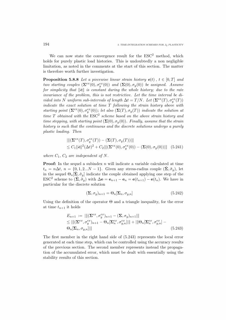
194 5. TIME-INTEGRATION SCHEMES FOR J2 PLASTICITY
We can now state the convergence result for the ESC2 method, whichholds for purely plastic load histories. This is undoubtedly a non negligiblelimitation, as noted in the comments at the start of this section. The matteris therefore worth further investigation.
Proposition 5.8.8 Let a piecewise linear strain history e(t) , t ∈ [0, T ] andtwo starting couples (Σex(0), σex
y (0)) and (Σ(0), σy(0)) be assigned. Assumefor simplicity that ‖e‖ is constant during the whole history; due to the rateinvariance of the problem, this is not restrictive. Let the time interval be di-vided into N uniform sub-intervals of length ∆t = T/N . Let (Σex(T ), σex
y (T ))indicate the exact solution at time T following the strain history above withstarting point (Σex(0), σex
y (0)); let also (Σ(T ), σy(T )) indicate the solution attime T obtained with the ESC2 scheme based on the above strain history andtime stepping, with starting point (Σ(0), σy(0)). Finally, assume that the strainhistory is such that the continuous and the discrete solutions undergo a purelyplastic loading. Then
|‖(Σex(T ), σexy (T ))− (Σ(T ), σy(T ))|‖
≤ C1‖e‖2(∆t)2 + C2|‖(Σex(0), σexy (0)) − (Σ(0), σy(0))|‖ (5.241)
where C1, C2 are independent of N .
Proof: In the sequel a subindex n will indicate a variable calculated at timetn = n∆t, n = 0, 1, 2...N − 1. Given any stress-radius couple (Σ, σy), letin the sequel Θn[Σ, σy] indicate the couple obtained applying one step of theESC2 scheme to (Σ, σy) with ∆e = en+1 − en = e(tn+1) − e(tn). We have inparticular for the discrete solution
(Σ, σy)n+1 = Θn[Σn, σy,n] (5.242)
Using the definition of the operator Θ and a triangle inequality, for the errorat time tn+1 it holds
En+1 := |‖(Σex, σexy )n+1 − (Σ, σy)n+1|‖
≤ |‖(Σex, σexy )n+1 −Θn[Σex
n , σexy,n]|‖+ |‖Θn[Σex
n , σexy,n]−
Θn[Σn, σy,n]|‖ (5.243)
The first member in the right hand side of (5.243) represents the local errorgenerated at each time step, which can be controlled using the accuracy resultsof the previous section. The second member represents instead the propaga-tion of the accumulated error, which must be dealt with essentially using thestability results of this section.
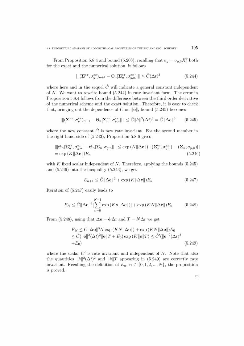
5.8. THEORETICAL ANALYSIS OF ALGORITHMICAL PROPERTIES OF THE ESC AND ESC2 SCHEMES 195
From Proposition 5.8.4 and bound (5.208), recalling that σy = σy,0Xq0 both
for the exact and the numerical solution, it follows
|‖(Σex, σexy )n+1 −Θn[Σex
n , σexy,n]|‖ ≤ C(∆t)3 (5.244)
where here and in the sequel C will indicate a general constant independentof N . We want to rewrite bound (5.244) in rate invariant form. The error inProposition 5.8.4 follows from the difference between the third order derivativeof the numerical scheme and the exact solution. Therefore, it is easy to checkthat, bringing out the dependence of C on ‖e‖, bound (5.245) becomes
|‖(Σex, σexy )n+1 −Θn[Σex
n , σexy,n]|‖ ≤ C‖e‖3(∆t)3 = C‖∆e‖3 (5.245)
where the new constant C is now rate invariant. For the second member inthe right hand side of (5.243), Proposition 5.8.6 gives
|‖Θn[Σexn , σ
exy,n]−Θn[Σn, σy,n]|‖ ≤ exp (K‖∆e‖)|‖(Σex
n , σexy,n)− (Σn, σy,n)|‖
= exp (K‖∆e‖)En (5.246)
with K fixed scalar independent of N . Therefore, applying the bounds (5.245)and (5.246) into the inequality (5.243), we get
En+1 ≤ C‖∆e‖3 + exp (K‖∆e‖)En (5.247)
Iteration of (5.247) easily leads to
EN ≤ C‖∆e‖3[N−1∑n=0
exp (Kn‖∆e‖)] + exp (KN‖∆e‖)E0 (5.248)
From (5.248), using that ∆e = e ∆t and T = N∆t we get
EN ≤ C‖∆e‖3N exp (KN‖∆e‖) + exp (KN‖∆e‖)E0
≤ C(‖e‖2(∆t)2‖e‖T + E0) exp (K‖e‖T ) ≤ C ′(‖e‖2(∆t)2
+E0) (5.249)
where the scalar C ′ is rate invariant and independent of N . Note that alsothe quantities ‖e‖2(∆t)2 and ‖e‖T appearing in (5.249) are correctly rateinvariant. Recalling the definition of En, n ∈ 0, 1, 2, ..., N, the propositionis proved.

196 5. TIME-INTEGRATION SCHEMES FOR J2 PLASTICITY
Remark 5.8.9 The convergence result for the ESC method is not restricted topurely plastic load histories. The result is identic to that of Proposition 5.8.8but holding for any type of loading history. The proof is essentially the sameas for Proposition 5.8.8 but using the more general Proposition 5.8.5 insteadof Proposition 5.8.6.
In the following the reader is provided with the proofs of the lemmas recalledin Section 5.8.5 devoted to the numerical analysis of the exponential-basedalgorithms. The present results which play a key role in the derivations carriedout in the previous section are taken from [11].
5.8.6 Two lemmas
We now introduce and prove the two lemmas mentioned in the previous sec-tions by first recalling the following identities which can be derived from thenew formulation of Section 5.7.1. At all time instants during plastic steps itholds:
Xs = σ−1y,0 X
1−q0 Σ (5.250)
Σ = σy,0 Xq−10 Xs (5.251)
Lemma 5.8.10 Let two initial couples (Σ(t0), σy(t0)), (Σ(t0), σy(t0)) and astrain increment ∆e = e∆t be assigned. Assume to apply one step of the ESCor ESC2 algorithm with strain increment ∆e to both initial couples and assumethat both steps are totally plastic. Then at all instants t ∈ [t0, t0 + ∆t] duringthe time step, it holds
d
dt‖|Σ(t)− Σ(t), σy(t)− σy(t)‖|
≤ ‖e‖[K1‖|Σ(t0)− Σ(t0), σy(t0)− σy(t0)‖|
+ K2‖|Σ(t)− Σ(t), σy(t)− σy(t)‖|]
(5.252)
where the positive constants K1,K2, depending only on the material constantsand ‖∆e‖, are bounded on all sets of the type ∆e ∈ Lin, ‖∆e‖ ≤ c, c ∈ R+
Proof: The proof will be shown only in the case of the ESC2 algorithm.The proof for the ESC scheme is a simpler version of the one that follows andcan be trivially derived following the same steps. In the sequel, in order to

5.8. THEORETICAL ANALYSIS OF ALGORITHMICAL PROPERTIES OF THE ESC AND ESC2 SCHEMES 197
shorten the notation, the dependence of the variables on time will not be ex-plicited; unless differently noted, the time dependent equations and identitiesthat follow are valid for all t ∈ [t0, t0 + ∆t].
We will again adopt the notation introduced in (5.229). Direct derivationgives
d
dt‖|ΣE , σE
y ‖|2 = 2[(2G)−1(ΣE, Σ
E) + (Hiso)−1σE
y σEy
](5.253)
Deriving in time definition (5.251) and using (5.124)-(5.250) we easily get,without showing all the calculations,
ΣE
=d
dt(Σ− Σ) = σy,0T1 + T2 (5.254)
T1 =[2GRXq
0 −2GRXq
0
]e (5.255)
T2 = (q − 1)[2GR
(e : Σ)Σσy− 2G
R
(e : Σ
) Σσy
](5.256)
As a consequence, the first member in the right hand side of (5.253) can bebounded with
(2G)−1ΣE : ΣE
= (2G)−1 [σy,0 T1 + T2] : ΣE ≤ C (‖T1‖+ ‖T2‖) ‖ΣE‖(5.257)
where here and in the sequel C indicates a general positive constant dependingonly on the material constants. We now have
‖T1‖ ≤ C
[∣∣∣∣∣ R−RR RXq
0 +1R
(Xq
0 − Xq0
)∣∣∣∣∣]‖e‖
≤ C(∣∣∣∣∣R−RR R
Xq0
∣∣∣∣∣+∣∣∣∣ 1R (Xq
0 − Xq0)∣∣∣∣)‖e‖
= (A1 +A2)‖e‖ (5.258)
The definition of R, recalling that both couples are undergoing a purely plasticstep, becomes
R =‖Σi‖
c−1 ln (1 + c)(5.259)
c =2G q Σi : ∆e‖Σi‖2
(5.260)

198 5. TIME-INTEGRATION SCHEMES FOR J2 PLASTICITY
and the analogous for the barred variables. Therefore R is a real C1 functionof Σi.
Recalling that both couples are in plastic phase, it follows immediatelythat both ‖Σi‖ and ‖Σi‖ are greater or equal to σy,0. It is therefore easy tocheck that it exists a smooth path γ in Linsym from Σi to Σi such that
γ : [0, L] −→ Linsym (5.261)‖∇γ(s)‖ = 1 ∀s ∈ [0, L] (5.262)‖γ(s)‖ ≥ σy,0 ∀s ∈ [0, L] (5.263)L ≤ 4‖Σi − Σi‖ (5.264)
Note that the above conditions simply mean that γ is a C1 path of length Llesser than 4‖Σi − Σi‖, written with respect to its curvilinear abscissae andbounded outside a sphere of radius σy,0 centered at the origin.
From the Lagrange theorem applied to the function R(Σ) along the pathγ, it follows the existence of β ∈ [0, L] such that
R− R = L∇R|Σ∗i
: ∇γ|β (5.265)
where
Σ∗i = γ(β) 0 ≤ β ≤ L (5.266)
Using (5.262) and (5.264), from (5.265) we get
|R− R| ≤ 4‖∇R|Σ∗i‖ ‖Σi − Σi‖ (5.267)
Substituting (5.267) in the definition of A1 and using the Cauchy-Schwartzinequality now leads to
A1 ≤‖∇R|Σ∗
i‖
R
Xq0
R‖Σi − Σi‖ (5.268)
We now want to bound the pieces in (5.268). A direct calculation gives
∇R|Σ∗i
=1
c−1 ln (1 + c)∇‖Σ‖ − ‖Σ∗
i ‖
1c(1 + c)
−ln (1 + c)
c2
(c−1 ln (1 + c))2
[∂c
∂Σ
](5.269)
where all the functions and derivatives are calculated in Σ∗i . We note that the
functions
1c(1 + c)
− ln (1 + c)c2
, c−1 ln (1 + c) (5.270)

5.8. THEORETICAL ANALYSIS OF ALGORITHMICAL PROPERTIES OF THE ESC AND ESC2 SCHEMES 199
are bounded from above on all the positive real line. Also, recalling (5.260), itis easy to check that the latter function c−1 ln (1 + c) is bounded from belowby a positive constant (independent of ‖Σ∗
i ‖) on all sets of the type ∆e ∈Lin, ‖∆e‖ ≤ c, c ∈ R+. A direct calculation also easily gives
‖[∂c
∂Σ
]|Σ∗
i‖ ≤ C ‖∆e‖
‖Σ∗i ‖2
(5.271)
Joining the latter three statements with (5.269) and noting that the normof ∇(‖Σ‖) is equal to one, gives
‖∇R|Σ∗i‖ ≤ K ′
3
(1 + ‖Σ∗
i ‖−1)
(5.272)
where K ′3 depends only on ‖∆e‖ and is bounded on all sets of the type ∆e ∈
Lin, ‖∆e‖ ≤ c, c ∈ R+. Finally, due to definition (5.266) and condition(5.263), the above bound becomes
‖∇R|Σ∗i‖ ≤ K3 (5.273)
where K3 depends only on ‖∆e‖ and is bounded on all sets of the type ∆e ∈Lin, ‖∆e‖ ≤ c, c ∈ R+.
Using again the boundedness from above of c−1 ln (1 + c) and recalling(5.259), (5.156) we have
1R≤ c−1 ln (1 + c)
σy,0≤ C (5.274)
1R
=c−1 ln (1 + c)σy,0X
q0,i
≤ C 1Xq
0,i
(5.275)
Using (5.275) and recalling that X0 never decreases during the step, we nowhave
Xq0
R≤ C
(X0
X0,i
)q
≤ C(X0,f
X0,i
)q
(5.276)
We observe that, due to (5.143)-(5.145) and recalling that
‖Xs‖ = X0 during plastic phases (5.277)
it follows
X0,f = be : Xs
i
‖e‖ + aX0,i ≤ b‖Xsi‖+ aX0,i ≤ (b+ a)X0,i (5.278)

200 5. TIME-INTEGRATION SCHEMES FOR J2 PLASTICITY
Therefore, from (5.276) and (5.278), it holds
Xq0
R≤ C(b+ a)q ≤ C exp
(2G q
R‖∆e‖
)≤ K4 (5.279)
with K4 bounded on all sets of the type ∆e ∈ Lin, ‖∆e‖ ≤ c, c ∈ R+.Finally, simply applying the three bounds (5.273),(5.274) and (5.279) into
(5.268), we obtain
A1 ≤ K5‖Σi − Σi‖ (5.280)
with K5 depending only on ∆e and bounded on all sets of the type ∆e ∈Lin, ‖∆e‖ ≤ c, c ∈ R+. Using (5.274) and observing that any difference oftensor norms is bounded by the norm of the difference, we get for the secondterm in (5.258)
A2 =∣∣∣∣ 1Rσ−1
y,0
(‖Σ‖ − ‖Σ‖
)∣∣∣∣ ≤ C (‖Σ‖ − ‖Σ‖) ≤ C‖Σ− Σ‖ (5.281)
Applying the bounds (5.280) and (5.281) to (5.258), it immediately follows
‖T1‖ ≤ ‖e‖[K5‖Σi − Σi‖+ C‖Σ− Σ‖
](5.282)
The second term T2 is bound following the same techniques; in the end weobtain a similar bound
‖T2‖ ≤ ‖e‖[K6‖Σi − Σi‖+K7‖Σ − Σ‖
](5.283)
where K6,K7 depend only on ‖∆e‖ and are bounded on all sets of the type∆e ∈ Lin, ‖∆e‖ ≤ c, c ∈ R+.
For the second term in (5.253), using the identities (5.156) and (5.128), itfollows
|σE σE| = |σy − σy| σy,0 |Xq−10 X0 − Xq−1
0˙X0| (5.284)
which, recalling that in plastic phase σy = ‖Σ‖, becomes
|σE σE| ≤ C‖Σ− Σ‖ σy,0 |Xq−10 X0 − Xq−1
0˙X0| (5.285)
Applying identity (5.250), bound (5.285) becomes
|σE σE | ≤ C‖Σ− Σ‖(
2GR
e : Σ− 2GR
e : Σ)
(5.286)

5.8. THEORETICAL ANALYSIS OF ALGORITHMICAL PROPERTIES OF THE ESC AND ESC2 SCHEMES 201
where the term in parentheses can be bounded with the usual techniques.Thus it is found that
|σE σE | ≤ ‖Σ− Σ‖ ‖e‖[K10‖Σi − Σi‖+K11‖Σ− Σ‖
](5.287)
where K10,K11 share the usual property of the previous cases.Simply applying the four bounds (5.257), (5.282), (5.283) and (5.287) into
(5.253), we obtain
d
dt‖|ΣE(t), σy(t)E‖|2 ≤ ‖e‖
[K1‖Σi − Σi‖+K2‖Σ− Σ‖
]‖ΣE‖
≤ C‖e‖[K1‖Σi − Σi‖+K2‖Σ − Σ‖
]‖|ΣE(t), σy(t)E‖| (5.288)
where K1,K2 depend only on ‖∆e‖ and are bounded on all sets of the type∆e ∈ Lin, ‖∆e‖ ≤ c, c ∈ R+. Observing that
d
dt‖|ΣE(t), σy(t)E‖|2 = 2‖|ΣE(t), σy(t)E‖|
d
dt‖|ΣE(t), σy(t)E‖| (5.289)
bound (5.288) trivially proves the lemma.
Lemma 5.8.11 Let two initial couples (Σ(t0), σy(t0)), (Σ(t0), σy(t0)) and astrain increment ∆e = e∆t be assigned. Assume to apply one step of theESC algorithm with strain increment ∆e to both initial couples; assume alsothat the step for the first couple is totally plastic, while the step for the secondcouple is totally elastic. Then at all instants t ∈ [t0, t0 + ∆t] during the timestep, it holds
d
dt‖|Σ(t)− Σ(t), σy(t)− σy(t)‖|
≤ ‖e‖[K1‖|Σ(t0)− Σ(t0), σy(t0)− σy(t0)‖|
+K2 ‖|Σ(t)− Σ(t), σy(t)− σy(t)‖|]
(5.290)
where the positive constants K1,K2 depend only on ‖∆e‖ and are bounded onall sets of the type ∆e ∈ Lin, ‖∆e‖ ≤ c, c ∈ R+
Proof: As in the proof of Lemma 5.8.10, the dependence of the variableson time will not be explicited. Unless differently noted, the time dependentequations and identities that follow are valid for all t ∈ [t0, t0 + ∆t].

202 5. TIME-INTEGRATION SCHEMES FOR J2 PLASTICITY
We will again adopt the notation introduced in (5.229). Following the sameidentical initial steps as in Lemma 5.8.10, we get
d
dt‖|ΣE , σE
y ‖|2 = 2[(2G)−1 ΣE : Σ
E+ (Hiso)−1σE
y σy
](5.291)
where we implicitly used that σEy = σy because the second couple is in elastic
phase. Note that for the time derivative of X, which is in elastic phase, itholds
d
dtX
s=
2Gσy,i
X0e (5.292)
d
dtX0 = 0 (5.293)
while the time derivative of X still follows (5.124)-(5.250). Deriving in timedefinition (5.251), then using (5.124)-(5.250) and (5.292)-(5.293), we easily get,without showing all the calculations,
ΣE
=d
dt(Σ− Σ) = σy,0 T1 + T2 (5.294)
T1 =[
2Gσy,i
Xq0 −
2Gσy,i
Xq0
]e (5.295)
T2 = (q − 1)[2GR
(e : Σ)Σσy
](5.296)
Joining (5.291) and (5.294) gives
d
dt‖|ΣE , σE
y ‖|2 = 2(2G)−1σy,0 T1 : ΣE
+2[(2G)−1T2 : ΣE + (Hiso)−1σE
y σy
]=: A1 +A2 (5.297)
Recalling the identity (5.156), which holds in all phases and using that σy =σy,i during all the step, we get
A1 = 2
(σy
σy,i− 1
)e : ΣE ≤ 2
σy,i|σy − σy,i| ‖ΣE‖ ‖e‖ (5.298)
Observing that σy,i ≥ σy,0 and σy = σy,i, due to a triangle inequality it follows
A1 ≤2σy,0
(|σy − σy|+ |σy,i − σy,i|) ‖ΣE‖ ‖e‖ (5.299)

5.8. THEORETICAL ANALYSIS OF ALGORITHMICAL PROPERTIES OF THE ESC AND ESC2 SCHEMES 203
which, from definition (5.227), becomes
A1 ≤ C(‖|ΣE
i , σEy,i‖|+ ‖|ΣE, σE
y ‖|)‖|ΣE , σE
y ‖| ‖e‖ (5.300)
where the scalar C depends only on the material constants.Deriving in time and applying (5.128) we get
σy =d
dt[σy,0X
q0 ] = q σy,0 X
q−10 X0 = q σy,0 X
q−10
2Gσy,i
e : Xs (5.301)
Applying (5.156) and (5.250), the identity above easily gives
σy = q2Gσy,i
e : Σ (5.302)
From the definition of q (see (5.156)), identity (5.302) and rearranging theterms, the second member in (5.297) becomes
A2 =[−2
2G2G+Hiso
Σσy
: ΣE + 22G
2G+HisoσE
y
]e : Σσy,i
= 22G
2G+Hiso
[−Σσy
: ΣE + σy − σy
]e : Σσy,i
(5.303)
which we will show being lesser or equal than zero. Note that, being the firstcouple in purely plastic phase, e : Σ ≥ 0; as a consequence, in order to show
A2 ≤ 0 (5.304)
it is sufficient to show
−Σσy
: ΣE + σy − σy ≤ 0 (5.305)
Multiplying and dividing by σy, then recalling that ‖Σ‖ = σy, we get
−Σσy
: ΣE + σy − σy =1σy
[−‖Σ‖2 + Σ : Σ + σ2
y − σyσy
](5.306)
=1σy
[Σ : Σ− σyσy
]A Cauchy-Schwarz inequality and the Kuhn-Tucker conditions applied to (5.306)then give
−Σσy
: ΣE + σy − σy ≤1σy
[‖Σ‖‖Σ‖ − σyσy] ≤ 0 (5.307)
which implies (5.304). Joining (5.300) and (5.304) with (5.297) implies
d
dt‖|ΣE, σE
y ‖|2 ≤ C(‖|ΣE
i , σEy,i‖|+ ‖|ΣE , σE
y ‖|)‖|ΣE , σE
y ‖| ‖e‖ (5.308)
which recalling (5.289) easily proves the Lemma.

204 5. TIME-INTEGRATION SCHEMES FOR J2 PLASTICITY
5.9 NLK plasticity model
We start by recalling the associative von-Mises plasticity model under conside-ration, already examined in Section 2.3.3 and labeled as NLK model. Splittingthe strain and stress tensors, σ and εεε, in deviatoric and volumetric parts wehave
σ = s + pI with p =13tr(σ) (5.309)
εεε = e +13θI with θ = tr(εεε) (5.310)
where tr indicates the trace operator, while I, s, p, e, θ are respectively thesecond-order identity tensor, the deviatoric and volumetric stress, the devia-toric and volumetric strain.
The equations for the model are
p = Kθ (5.311)s = 2G[e− ep] (5.312)Σ = s−α (5.313)F = ‖Σ‖ − σy (5.314)ep = γn (5.315)σy = σy,0 +Hisoγ (5.316)α = Hkinγn−Hnlγα (5.317)γ ≥ 0 , F ≤ 0 , γF = 0 (5.318)
where K is the material bulk elastic modulus, G is the material shear mod-ulus, ep is the traceless plastic strain, Σ is the relative stress in terms ofthe backstress α, the latter introduced to describe the nonlinear kinematichardening mechanism. Moreover, F is the von-Mises yield function, n is thenormal to the yield surface, σy is the yield surface radius, σy,0 the initial yieldstress, Hkin and Hiso are the kinematic and isotropic linear hardening moduli.The constant Hnl is the nonlinear kinematic hardening modulus, introducedto represent a nonlinear kinematic hardening mechanism (see Section 2.3.2).Finally, Equations (5.318) are the Kuhn-Tucker conditions; in particular, thesecond equation limits the relative stress within the boundary defined by theyield surface F = 0, while the other two are necessary to determine the plasticbehavior. With a slight over-simplification of the model complexity, we maysay that when γ = 0 the system is in an elastic phase, while when γ > 0 wesay that the system is in a plastic phase.

5.10. BACKWARD EULER’S INTEGRATION SCHEME FOR THE NLK MODEL 205
In the following sections a set of numerical schemes for the above problemis presented. The first two schemes are based respectively on the backwardEuler’s and on the generalized midpoint integration rules, while the third oneis a newly developed exponential-based integration algorithm.
Remark 5.9.1 Due to the linear behavior of the volumetric part constitutiveequations, in the following we treat only the deviatoric part of the model.
5.10 Backward Euler’s integration scheme for theNLK model
In this section we present a numerical method which uses a backward Euler’sintegration rule and is combined with a return map algorithm. Originallyproposed in the context of elasoplastic models by Maenchen and Sack [59] byWilkins [76], by Auricchio and Taylor [17] in the framework of generalizedplasticity, the return map algorithm is based on the elastic predictor- plasticcorrector strategy. The return map is achieved enforcing consistency at theend of the time step and projecting the trial solution onto the updated yieldsurface at the end of each elastoplastic step. This procedure result in solvinga fourth-order polynomial in the plastic consistency parameter. As usual, wepresent both the time integration and the solution algorithm together withthe consistent elastoplastic tangent operator. In the following the presentscheme is referred to as BEnl (Backward-Euler integration method for von-Mises plasticity with nonlinear hardening).
It is assumed that the time history interval [0, T ] is divided into N sub-intervals defined by the nodes 0 = t0 < t1 < .... < tn < tn+1 < .... < tN = T .Given the values sn, en, e
pn, γn,αn at time tn, and the deviatoric strain en+1
at time tn+1, the scheme consists in computing the remaining variables at timetn+1. The strain history is assumed to be piecewise linear and the initial valuesof γ, ep and α are equal to zero.
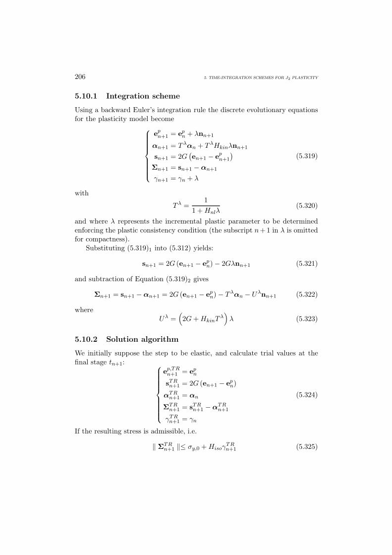
206 5. TIME-INTEGRATION SCHEMES FOR J2 PLASTICITY
5.10.1 Integration scheme
Using a backward Euler’s integration rule the discrete evolutionary equationsfor the plasticity model become
epn+1 = ep
n + λnn+1
αn+1 = T λαn + T λHkinλnn+1
sn+1 = 2G(en+1 − ep
n+1
)Σn+1 = sn+1 −αn+1
γn+1 = γn + λ
(5.319)
with
T λ =1
1 +Hnlλ(5.320)
and where λ represents the incremental plastic parameter to be determinedenforcing the plastic consistency condition (the subscript n+1 in λ is omittedfor compactness).
Substituting (5.319)1 into (5.312) yields:
sn+1 = 2G (en+1 − epn)− 2Gλnn+1 (5.321)
and subtraction of Equation (5.319)2 gives
Σn+1 = sn+1 −αn+1 = 2G (en+1 − epn)− T λαn − Uλnn+1 (5.322)
whereUλ =
(2G+HkinT
λ)λ (5.323)
5.10.2 Solution algorithm
We initially suppose the step to be elastic, and calculate trial values at thefinal stage tn+1:
ep,TRn+1 = ep
n
sTRn+1 = 2G (en+1 − ep
n)
αTRn+1 = αn
ΣTRn+1 = sTR
n+1 −αTRn+1
γTRn+1 = γn
(5.324)
If the resulting stress is admissible, i.e.
‖ ΣTRn+1 ‖≤ σy,0 +Hisoγ
TRn+1 (5.325)

5.10. BACKWARD EULER’S INTEGRATION SCHEME FOR THE NLK MODEL 207
nT
, 1y n
,y n
n
1n
1nn
1
TR
ns
1ns
ns
O
Figure 5.4: Application of the return map algorithm to the BEnl integrationscheme. Plastic correction representation in deviatoric stress space.
the step is assumed to be elastic and the variable values at the final timeinstant are taken as the trial ones. On the other hand, if ΣTR
n+1 violates theyield limit, a plastic correction is introduced. Enforcing the satisfaction of thelimit equation permits to compute λ and thus the discrete equantions (5.326)can be rewritten in terms of the trial state and λ:
epn+1 = ep,TR
n + λnn+1
sn+1 = sTRn+1 − 2Gλnn+1
αn+1 = T λαTRn+1 +HkinT
λλnn+1
Σn+1 = sTRn+1 − T λαTR
n+1 − Uλnn+1
γn+1 = γTRn+1 + λ
(5.326)
A graphical idealization of the return map algorithm applied to the BEnlintegration scheme is provided in Figure 5.4 which represents in the devia-toric stress space the trial elastic predictor and the plastic corrector obtainedapplying the return map algorithm to the BEnl scheme.
It is noted that in Equations (5.319) and (5.326) the only unknown isrepresented by the consistency parameter λ which is to be computed imposingyield consistency at the end of the step. Therefore, the above sequential updateprocedure is set forth by enforcing the plastic consistency condition at tn+1 bymeans of a return map algorithm.
Observing that (5.326)4 can be rewritten as
Σn+1 = ΣλA − Uλnn+1 (5.327)
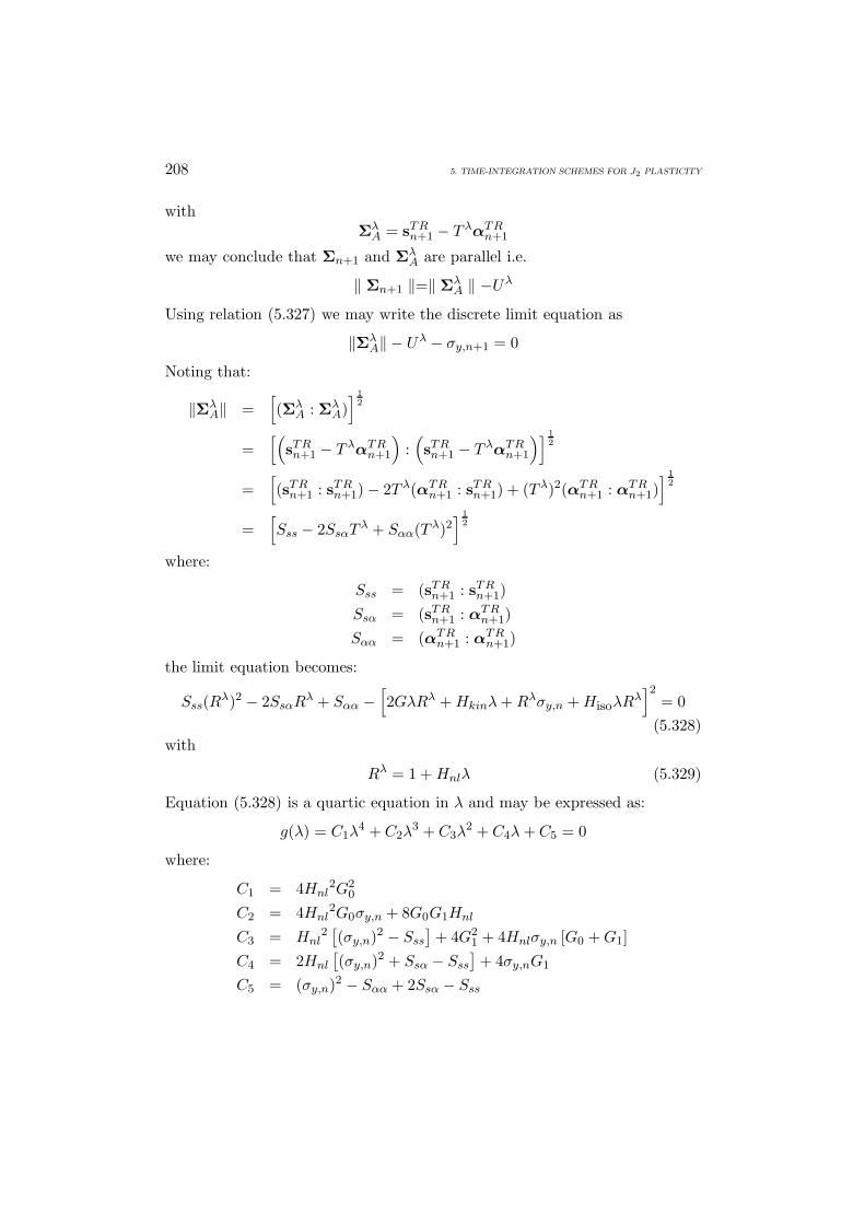
208 5. TIME-INTEGRATION SCHEMES FOR J2 PLASTICITY
withΣλ
A = sTRn+1 − T λαTR
n+1
we may conclude that Σn+1 and ΣλA are parallel i.e.
‖ Σn+1 ‖=‖ ΣλA ‖ −Uλ
Using relation (5.327) we may write the discrete limit equation as
‖ΣλA‖ − Uλ − σy,n+1 = 0
Noting that:
‖ΣλA‖ =
[(Σλ
A : ΣλA)] 1
2
=[(
sTRn+1 − T λαTR
n+1
):(sTRn+1 − T λαTR
n+1
)] 12
=[(sTR
n+1 : sTRn+1)− 2T λ(αTR
n+1 : sTRn+1) + (T λ)2(αTR
n+1 : αTRn+1)
] 12
=[Sss − 2SsαT
λ + Sαα(T λ)2] 1
2
where:
Sss = (sTRn+1 : sTR
n+1)Ssα = (sTR
n+1 : αTRn+1)
Sαα = (αTRn+1 : αTR
n+1)
the limit equation becomes:
Sss(Rλ)2 − 2SsαRλ + Sαα −
[2GλRλ +Hkinλ+Rλσy,n +HisoλR
λ]2
= 0(5.328)
with
Rλ = 1 +Hnlλ (5.329)
Equation (5.328) is a quartic equation in λ and may be expressed as:
g(λ) = C1λ4 + C2λ
3 + C3λ2 + C4λ+C5 = 0
where:
C1 = 4Hnl2G2
0
C2 = 4Hnl2G0σy,n + 8G0G1Hnl
C3 = Hnl2[(σy,n)2 − Sss
]+ 4G2
1 + 4Hnlσy,n [G0 +G1]C4 = 2Hnl
[(σy,n)2 + Ssα − Sss
]+ 4σy,nG1
C5 = (σy,n)2 − Sαα + 2Ssα − Sss

5.10. BACKWARD EULER’S INTEGRATION SCHEME FOR THE NLK MODEL 209
with:2G0 = 2G+Hiso
The solution of this equation, i.e. the search for the minimum positive root, isnot an easy task, due to the order of the polynomial and to the dependence ofthe coefficients on the trial state. As observed in [17], an iterative algorithmof the Newton type may be easily implemented:
λi+1 = λi + ∆λi
∆λi = −g(λi)
g′ (λi)
where: the superscript i refers to the i-th iteration, the superscript ′ indicatesfirst derivative; and where a starting value of λ0 = 0 may be adopted. Unfor-tunately, this approach does not guarantee convergence to a positive root; infact:
∆λ(0) = − g(0)g′(0)
= −C5
C4
=ΣTR : ΣTR − (σy,n)2
2Hnl
[ΣTR : ΣTR − (σy,n)2
]+ 2Hnl(ΣTR : αTR)− 4σy,nG1
and the sign of ∆λ at zero depends on the sign of the denominator, whichclearly depends on the trial state and on the previous solution. Consequently,it may happen that ∆λ(0) < 0 and the Newton algorithm returns a negativevalue for λ. Attempts of starting the Newton iteration algorithm with differentvalues of λ (such as λ0 = λn) have been explored but generate the samepathology. Once the Newton algorithm has failed, the only robust approachis to perform a synthetic division of the quartic polynomial and compute inclosed form the roots of the resulting cubic [14]; the roots should then becorrected using a Newton algorithm, since the synthetic division is sensitiveto roundoff.
Remark 5.10.1 The NLK model has been used to simulate the behavior ofmetals under cyclic loading, achieving an high degree of accuracy. Moreover,extensions of the model to include strain range memory, visco-plastic recoveryproperties, ratcheting effects have been presented in the literature [17, 23, 69,70].
However, difficulties arise to implement the model in a return map frame-work and they are all directly related to the non-linear kinematic hardeningterm. The discrete consistency condition yields a quartic equation, whose co-efficients are function of the trial state and the previous solution, which makes

210 5. TIME-INTEGRATION SCHEMES FOR J2 PLASTICITY
difficult the search of the minimum positive root. An approach based on acombination of Newton’s algorithm and synthetic division is presented, whichis robust but at the same time computationally expensive. Moreover, the elasto-plastic tangent tensor consistent with the discrete model is non-symmetric and,as a result, an appropriate solver for non-symmetric linear systems must beused, plus the required memory storage is doubled.
5.10.3 BEnl scheme elastoplastic consistent tangent operator
We show here the consistent tangent operator for the BEnl scheme. Forbrevity’s sake, only the final form of the operator corresponding to a pla-stic step (i.e. such that λ = 0) is reported without deriving it thoroughly. Tomake notation more clear, the subscripts of all history variables evaluated attime tn+1 are omitted for brevity. Quantities evaluated either at tn are spec-ified by the relative subscript. The reader is referred to [17] for a completederivation.
Cep =
∂σ
∂εεε= KI⊗ I + 2G (1− C) Idev
+ [2G (C −A) +B (n : α)]n⊗ n−Bα⊗ n (5.330)
with
A =2G
2G0 + T λHkin − T λ (n : α)
B = AT λCHnl
C =2Gλ
‖ ΣλA ‖
5.11 Generalized midpoint integration scheme forthe NLK model
In this section we present the numerical method already proposed by Ortizand Popov [63] in the framework of linear hardening elastoplastic constitu-tive models. The method is based on a generalized midpoint integration rulecombined with a return map algorithm. The return map is achieved enforcingconsistency at the end of the time step and projecting the trial solution ontothe updated yield surface at the end of each elastoplastic step. This procedureresults in solving a 10th-order polynomial in the plastic consistency parameterwhich makes the computational effort quite significant. Again, this is still dueto the nonlinear kinematic hardening term.

5.11. GENERALIZED MIDPOINT INTEGRATION SCHEME FOR THE NLK MODEL 211
The present scheme is referred to as the MPTnl method (midpoint integra-tion method for von-Mises plasticity with nonlinear hardening). In particular,the generalized midpoint integration rule investigated herein can be special-ized to two different methods, namely the proper midpoint integration scheme[72] and the BEnl integration scheme analyzed in the preceding section. Themethod is outlined with its algorithmic solution sketch and consistent tangentoperator.
To the author’s knowledge, the literature does not report any detaileddevelopment or testing of the midpoint method MPTnl for the von-Mises pla-sticity model with nonlinear hardening as the one considered here (see [13] fora detailed comparison of generalized midpoint integration procedures appliedto von-Mises plasticity with nonlinear hardening).
In the sequel it is assumed that the time history interval [0, T ] is dividedinto N sub-intervals defined by the nodes 0 = t0 < t1 < .... < tn < tn+1 <.... < tN = T . Given the values sn, en, γn,αn at time tn, and the deviatoricstrain en+1 at time tn+1, the scheme consists in computing the remainingvariables at time tn+1. The strain history is assumed to be piecewise linearand the initial values of γ, ep and α are zero.
5.11.1 Integration scheme
Using a generalized midpoint integration rule the discrete evolutionary equa-tions can be written as:
epn+1 = ep
n + λnn+α
αn+1 = αn + λ (Hkinnn+α −Hnlαn+α)sn+1 = 2G
(en+1 − ep
n+1
)Σn+1 = sn+1 −αn+1
γn+1 = γn + λ
(5.331)
where λ represents the incremental plastic parameter to be determined enforc-ing the plastic consistency condition. The scalar α is the algorithmic parametersuch that the following relations hold for quantities evaluated at the midpointinstant tn+α
en+α = αen+1 + (1− α)en
epn+α = αep
n+1 + (1− α)epn
αn+α = ααn+1 + (1− α)αn
sn+α = 2G(en+α − ep
n+α
)Σn+α = sn+α −αn+α
(5.332)

212 5. TIME-INTEGRATION SCHEMES FOR J2 PLASTICITY
Clearly, α can be arbitrarily chosen in the range (0, 1]. In particular, in thefollowing we consider the possibility of α = 1/2, leading to the midpoint inte-gration rule (MPTnl). We remark that adopting α = 1 leads to the backwardEuler’s integration rule (BEnl). The difference between the two schemes laysin fact only in the choice of the α parameter. The choice α = 1/2 guaranteesquadratic accuracy to the MPTnl, while the choice α = 1 makes the BEnlmethod a simpler and more robust scheme with linear accuracy.
5.11.2 Solution algorithm
The elastic predictor-plastic corrector solution idea is applied again. Initially,the step is supposed to be elastic. This yields the following trial values at thefinal instant tn+1:
ep,TRn+1 = ep
n
sTRn+1 = 2G (en+1 − ep
n)
αTRn+1 = αn
ΣTRn+1 = sTR
n+1 −αTRn+1
γTRn+1 = γn
(5.333)
If the resulting relative stress is admissible, i.e.
‖ ΣTRn+1 ‖≤ σy,0 +Hisoγ
TRn+1 (5.334)
then the step is purely elastic and the history variables are updated with theirtrial values. On the other hand, if ΣTR
n+1 lays outside the yield surface, a plasticcorrection is introduced in two steps:
• STEP 1: update at tn+α.
αn+α = V λαTR
n+1 + αHkinVλλnn+α
sn+α = sTRn+α − 2Gαλnn+α
Σn+α = sn+α −αn+α
(5.335)
where
sTRn+α = 2G (en+α − ep
n)
V λ =1
1 + αHnlλ

5.11. GENERALIZED MIDPOINT INTEGRATION SCHEME FOR THE NLK MODEL 213
nV
n
,y n
, 1y n
,y n
n
1n
1nn
1
TR
ns
1nsns
O
TR
ns
nn
Figure 5.5: Application of the return map algorithm to the MPTnl integrationscheme. Plastic correction representation in deviatoric stress space.
• STEP 2: update at tn+1.
epn+1 = ep
n + λnn+α
αn+1 = W λαn +HkinVλλnn+α
sn+1 = 2G(en+1 − ep
n+1
)Σn+1 = sn+1 −αn+1
γn+1 = γn + λ
(5.336)
with
W λ =1 + (α− 1)λHnl
1 + αλHnl
Remark 5.11.1 In the case of the BEnl scheme, step (5.336) is equivalent to(5.335) and therefore is avoided in the procedure.
A graphical idealization of the return map algorithm applied to the MPTnlintegration scheme is provided in Figure 5.5, which represents in the devia-toric stress space the trial elastic predictor and the plastic corrector obtainedapplying the return map algorithm to the MPTnl scheme.
It is noted that in Equations (5.335) and (5.336) the only unknown isrepresented by the consistency parameter λ which is to be computed imposing

214 5. TIME-INTEGRATION SCHEMES FOR J2 PLASTICITY
yield consistency at the end of the step. Therefore, the above sequential updateprocedure is set forth by enforcing the plastic consistency condition at tn+1.Observing that (5.335)3 can be rewritten as
Σn+α = ΣλB − Y λnn+α (5.337)
with
ΣλB = sTR
n+α − V λαTRn+1
Y λ = 2Gαλ + αHkinVλλ
we may conclude that Σn+α and ΣλB are parallel i.e.
‖ Σn+α ‖=‖ ΣλB ‖ −Y λ (5.338)
Using relation (5.338) we can finally write the consistency condition at tn+1
as follows
‖ Σn+1 ‖=∥∥∥∥∥ 1αΣn+α −
(1− αα
)Σn
∥∥∥∥∥ = [σy,n + λHiso] (5.339)
Equation (5.339) is then solved searching for the minimum positive root. Notethat, as an alternative in solving the above equation, the yield condition (5.339)can be rewritten as
1α2‖ Σn+α ‖2 −2
(1− αα2
)(Σn+α : Σn)+
(1− αα
)2
‖ Σn ‖2= [σy,n + λHiso]2
(5.340)which, with some algebra, results in a 10th-order polynomial in λ. For brevity,the expression of the polynomial coefficients is here omitted.
Remark 5.11.2 In the case of the BEnl scheme, Equation (5.340) take asimpler form as the second and third term in the left hand side vanish. As aconsequence, the relevant polynomial in λ is fourth degree and the coefficientshave a shorter explicit form as discussed in Section 5.10.
Remark 5.11.3 Both th MPTnl and the BEnl scheme here presented are yieldconsistent and stable, as shown in [63] in a very general fashion. Moreover,the BEnl method is shown to be linearly accurate while the MPTnl method isquadratically accurate.
Remark 5.11.4 For the present model, the MPTnl midpoint scheme heredetailed is not guaranteed to have a solution for every trial sTR
n+1. On theother hand, from all the numerical tests carried out in Chapter 6, it seemsthat a solution always exists for the values of strain increment ‖ ∆e ‖ adoptedthroughout the testing.

5.11. GENERALIZED MIDPOINT INTEGRATION SCHEME FOR THE NLK MODEL 215
5.11.3 MPTnl scheme elastoplastic consistent tangent opera-tor
We report here the elastoplastic tangent operator consistent with the MPTnlscheme. For brevity’s sake, only the final form of the operator is given herefor a plastic step (i.e. such that λ = 0) without deriving it thoroughly. Tomake notation more clear, the subscripts of all history variables evaluated attime tn+1 are omitted for brevity. Quantities evaluated either at tn or at tn+α
are specified by the relative subscript.Following the derivation procedure reported in [17, 63, 71], the consistent
tangent operator∂σ
∂εfor the MPTnl scheme is easily obtained. Recalling that
∂s∂ε
=∂s∂e
∂e∂ε
=∂s∂e
Idev (5.341)
where
Idev = I− 13
(I⊗ I) (5.342)
and taking into account the volumetric part of the stress, from equations(5.309), (5.310) and (5.311) we get
Cep =
∂σ
∂ε=∂s∂e
Idev +K (I⊗ I) (5.343)
The fourth-order tensor∂s∂e
may be computed as
∂s∂e
= M1 + M2 (5.344)
where M1 and M2 are given by the following expressions
M1 = 2G(
I− η In − nn+α ⊗∂λ
∂e
)(5.345)
M2 = η In
(β ⊗ ∂λ
∂e
)(5.346)

216 5. TIME-INTEGRATION SCHEMES FOR J2 PLASTICITY
with
η = λ2G+HkinV
λ
2Gλ+HkinV λλ+ 2‖Σn+α‖(5.347)
In = I− nn+α ⊗ nn+α (5.348)
∂λ
∂e= −2G(θ1 + θ2)−1
(I−
2Gλ+HkinVλλ/2
2 ‖ sTRn+α − V λαn ‖
In
)Σ (5.349)
θ1 = Hisoσy,n+1 + (β : Σ) + 2G (nn+α : Σ) (5.350)
θ2 =Hnl
(2Gλ+HkinV
λλ/2)
2 (V λ)2(Σ : Inαn)
‖ sTRn+α − V λαn ‖
(5.351)
β =12Hnl
(V λ)2αn −
14Hkin
λHnl
(V λ)2nn+α +
12HkinV
λnn+α (5.352)
5.12 ESC2nl exponential-based integration schemefor the NLK model
In this section we propose an exponential-based numerical scheme for the NLKmodel. The method is based on a different formulation of the constitutiverelation and is developed following an ad-hoc rewriting of the time continuousmodel and on the application of exponential maps for the integration of therespective dynamical system [12]. A similar continuous formulation had beenadopted earlier by Hong and Liu [44, 46, 47] in the case of von Mises plasticmaterials with no hardening. The new algorithm here presented, which will bereferred as ESC2nl, represents an extension of previous algorithms introducedby the author et al. in the case of linear hardening [16, 8, 9, 10, 11] and is amember of the “ESC” integration schemes family.
As will be pointed out within the numerical test chapter the new ESC2nlscheme is yield consistent, quadratically accurate and grants exactness in caseof no hardening.
5.12.1 A model reformulation
Combining Equations (5.312) and (5.313), we obtain
Σ + α + 2Gep = 2Ge (5.353)
which, taking the derivative in time, applying Equation (5.315), (5.317) andrearranging terms gives
Σ = 2Ge− (2G+Hkin) ep +Hnlγα (5.354)

5.12. ESC2NL EXPONENTIAL-BASED INTEGRATION SCHEME FOR THE NLK MODEL 217
Now, recalling the yield surface radius
σy = σy,0 +Hisoγ (5.355)
and that in the plastic phase (γ > 0)
n =Σ‖Σ‖ =
Σσy,0 +Hisoγ
=Σσy
(5.356)
we may apply (5.315) in (5.354) obtaining
Σ + (2G +Hkin)Σσyγ = 2GΨ (5.357)
where we introduced the position
Ψ = e +Hnl
2Gγα (5.358)
Note that (5.357) is a differential equation for Σ that is valid also during elasticphases (γ = 0). Introducing the scaled relative stress
Σ :=Σσy
(5.359)
we observe that, whenever the relative stress Σ lays on the yield surface, thenΣ = n, while this is not true when Σ lays inside the yield surface. The timederivative of (5.359) and the use of relation (5.355) gives
˙Σ =Σσy− Hiso
σyγΣ (5.360)
Using Equations (5.357) and (5.360), one obtains
˙Σ +2G +Hkin +Hiso
σyγΣ =
2Gσy
Ψ (5.361)
The next goal is to introduce an integration factor for the above evolutionaryequation. In other words, we search for a scalar function depending on timeX0 such that
ddt
[X0Σ] = X0˙Σ + X0Σ = X0
˙Σ +X02G+Hkin +Hiso
σyγΣ (5.362)
which, multiplying Equation (5.361) by X0, would give
ddt[X0Σ
]=
2GσyX0Ψ (5.363)

218 5. TIME-INTEGRATION SCHEMES FOR J2 PLASTICITY
Accordingly, we set
X0(γ) =
(1 +
γHiso
σy,0
)2G+Hkin +Hiso
Hisoif Hiso = 0
exp
(2G+Hkin +Hiso
σy,0γ
)if Hiso = 0
(5.364)
Noting that such a function is continuous for fixed γ and Hiso → 0, and that
X0 =2G+Hkin +Hiso
σyγX0 (5.365)
we immediately obtain the target relationship (5.362) and therefore (5.363).We now need an evolution law for X0. In elastic phases, such law follows
immediately from (5.365):
X0 = 0 (elastic phases) (5.366)
On the other hand, for γ = 0, taking the scalar product of (5.363) with Σ,we have
X012
ddt‖Σ‖2 + X0‖Σ‖2 =
2GσyX0Ψ : Σ (5.367)
which, noting that in plastic phases
‖Σ‖ =‖Σ‖σy
= 1 (5.368)
and using (5.367) gives
X0 =2Gσy
Ψ : X0Σ (plastic phases) (5.369)
At this stage, we define the generalized stress X as the two componentvector represented in engineering notation as
X =X0ΣX0
=Xs
X0
(5.370)
As done for the ENN, ESC and ESC2 schemes, we consider a linear spacestructure on the space of generalized stresses, the product by a scalar and thesum between vectors being defined in the obvious natural way. Moreover, any

5.12. ESC2NL EXPONENTIAL-BASED INTEGRATION SCHEME FOR THE NLK MODEL 219
element of the space of linear operators from the generalized stress space intoitself can be written adopting the engineering notation as
[M] =[
M11 M12
M21 M22
](5.371)
with M11 a fourth-order tensor, M12,M21 second-order tensors and M22 ascalar, under the convention that the formal expression
MY (5.372)
returns a generalized stress vector given by the following operation
[M] Y =[
M11 M12
M21 M22
]Ys
Y0
=
M11Ys + M12Y0
M21 : Ys + M22Y0
(5.373)
for any couple Y = Ys, Y0T in the generalized stress space. In the sequel,we will consider a linear space structure also on the space of the linear operatorsacting on couples, again with the product by a scalar and the sum betweensuch linear operators being defined in the obvious natural way.
Due to definition (5.370), Equation (5.363) can be rewritten as
Xs
=2GσyX0Ψ (5.374)
while (5.369) becomes
X0 =2Gσy
Ψ : Xs (plastic phases) (5.375)
Equations (5.374), (5.366) and (5.375) provide a system for the generalizedstress vector X, in the form
X = AX (5.376)
where A represents a linear operator acting from the space of couples intoitself, and depending on the actual phase as follows
[A] = [Ae] =2Gσy
[O Ψ0 0
](elastic phase) (5.377)
[A] = [Ap] =2Gσy
[O ΨΨ 0
](plastic phase) (5.378)

220 5. TIME-INTEGRATION SCHEMES FOR J2 PLASTICITY
where 0 and O indicate respectively the second-order and fourth-order nulltensors.
Expression (5.376)-(5.378) is a formal compact notation to describe theaction of the linear operator A on the couple X, as introduced in (5.373).
Therefore the original problem, expressed by Equations (5.312)-(5.317),has been substituted by a new one, expressed by Equations (5.376)-(5.378).Note that Ψ can be equivalently substituted by e in (5.377), because γ = 0during elastic phases.
Remark 5.12.1 Unless Hiso = Hnl = 0, the operator A is not constant intime, therefore our formulation (5.376) is nonlinear. Nevertheless, the parti-cular form of the dynamical system (5.376) is useful, since it allows to developthe numerical method of Section 5.12.2.
Time-continuous on-off switch
To properly convert the original problem in a new but equivalent differentialalgebraic format, we also need to introduce an elastoplastic phase determina-tion criterion expressed in the new generalized stress environment.
For a given state to be plastic, the following two conditions must be fulfilled:
1) The relative stress Σ must be on the yield surface, i.e.
‖Σ‖ = σy (5.379)
Using (5.359) and (5.370) this can be easily rewritten as
‖Xs‖2 = ‖Σ‖2X20 =‖Σ‖2σ2
y
X20 = X2
0 (5.380)
2) The direction of the strain rate e must be outward with respect to theyield surface, i.e.
Σ : e > 0 (5.381)
Again recalling (5.359) and (5.370) it is immediate to check that (5.381)is equivalent to
Xs : e > 0 (5.382)
If the two conditions (5.380) and (5.382) are not satisfied, the step is elastic.

5.12. ESC2NL EXPONENTIAL-BASED INTEGRATION SCHEME FOR THE NLK MODEL 221
5.12.2 Integration scheme
It is assumed that the time history interval [0, T ] is divided into N sub-intervalsdefined by the points 0 = t0 < t1 < .... < tn < tn+1 < .... < tN = T . Given thevalues sn, en, γn,αn at time tn, and the deviatoric strain en+1 at time tn+1,we search for the remaining variables at time tn+1. As usual, the strain historyis assumed to be piecewise linear. Equivalently, we may say that the piecewiselinearity of the strain path makes e constant within each single time interval.Moreover, we assume to start from an unstressed and undeformed state, i.e.characterized by zero initial values of the variables γ, ep and α. Accordingly,the initial generalized stress is
X0 =Σ0/σy,0
1
(5.383)
Referring to the the dynamical law (5.376) with the operator A given respec-tively by (5.377) or (5.378), we aim to derive a numerical scheme for thediscrete evolution of X along the general time step [tn, tn+1].
It is immediate to observe that, if during the time interval [tn, tn+1] thematerial behavior is purely elastic (γ = 0 - elastic step), then the operator Ae
is constant within this interval. In this case, the dynamical law (5.376) can besolved in closed form and the formula (5.384) returns the exact solution. Inanalogy to (5.376), the discrete evolution of the generalized stress will be inthe form
Xn+1 = exp[A∆t
]Xn = G Xn (5.384)
with A = Ae and ∆t = tn+1 − tn. Note that, being A an element in the linearspace of linear operators acting on couples, the exponential of A∆t is naturallydefined by the (converging) exponential serie
exp[A∆t
]=
+∞∑n=0
(A∆t
)nn!
(5.385)
Instead, if during the step [tn, tn + 1] purely plastic loading takes place, thelinear operator Ap is not constant in time; in fact the yield surface radius σy
and the “driving” tensor Ψ cannot be expected to be constant whenever γ > 0(see Equations (5.316) and (5.358)). In such cases, therefore, the discretesolution of the dynamical system (5.376) is achieved by assuming that theabove variables remain constant within the time step. As a consequence, anequation identic to (5.384) still holds, clearly with a different choice of A.This is equivalent to substitute the operator Ap with an operator Ap whichis constant during the time step. The respective constant values taken by σy

222 5. TIME-INTEGRATION SCHEMES FOR J2 PLASTICITY
and Ψ, which depend on known quantities evaluated at the beginning of thestep tn, are still indicated by σy and ¯Ψ; we will specialize such constants inthe immediate following. Then, we may introduce A defined by
[Ae
]=
2Gσy,n
[O e0 0
](elastic step) (5.386)
and
[Ap
]=
2Gσy
[O
¯Ψ¯Ψ 0
](plastic step) (5.387)
We are now in possess of all the ingredients for solving the Equation (5.376).In particular the choice of the parameters σy and ¯Ψ for plastic steps is nowaddressed with emphasis on the effects this choices induces on the algorithmicalproperties.
The operator A∆t is by definition equal to the original operator (5.377)or (5.378) after substituting ¯Ψ with ∆Ψ = ∆t ¯Ψ and σy with σy. A possiblechoice is thus given by the following values
σy =cσy,n
ln(1 + c)
∆Ψ = ∆t ¯Ψ = ∆Ψ0 + ∆Ψ1
(5.388)
where the constant and tensors appearing in (5.388) are given by
c =2G q (nn : ∆e)
σy,n(5.389)
∆Ψ0 = ∆e +Hnl (nn : ∆e)
2G1 −Hnl (nn : αn)αn (5.390)
∆Ψ1 =12Hnl
2G(DαDγ +D′
γαn
)(5.391)

5.12. ESC2NL EXPONENTIAL-BASED INTEGRATION SCHEME FOR THE NLK MODEL 223
with
∆e = e∆t
q =Hiso
2G1 −Hnl (nn : αn)
nn =Xs
n
X0,n
2G1 = 2G+Hiso +Hkin
Dγ =2G
2G1 −Hnl (nn : αn)(nn : ∆e)
Dα = (Hkinnn −Hnlα)Dγ
D′γ =
2G2G1 −Hnl (nn : αn)
(Dn : ∆e)
+HnlDγ
2G1 −Hnl (nn : αn)[(Dn : αn) + (nn : Dα)]
Dn =2Gσy,n
∆e− 2G1Dγ
σy,nnn +
HnlDγ
σy,nDα
The choice for σy in (5.388) corresponds to an extension of the ESC2 schemepresented in Section 5.7 [9]. Instead, the value for ∆Ψ is essentially derivedfrom a first order expansion of the tensor Ψ in time. This choice guarantees asecond-order scheme as well as other properties as discussed in the sequel (see[12] for further details on this issue).
The linear operator G appearing in Equation (5.384) can be derived calcu-lating the shown exponential. Note that, for such purpose, it is convenient toreformulate the linear operator A∆t as a R7×7 matrix, calculate the exponen-tial, and finally write it back in the original form (5.371). Without showingthe calculations, we get
[G]
=
[Ge
]=
I2Gσy
∆e
0 1
(elastic step)
[Gp
]=
I +[(a− 1)‖∆Ψ‖2
]∆Ψ⊗∆Ψ b
∆Ψ‖∆Ψ‖
b∆ΨT
‖∆Ψ‖ a
(plastic step)
(5.392)

224 5. TIME-INTEGRATION SCHEMES FOR J2 PLASTICITY
where I is the fourth-order identity tensor, while the scalars a and b are
a = cosh(
2Gσy‖∆Ψ‖
)(5.393)
b = sinh(
2Gσy‖∆Ψ‖
)(5.394)
Another point to be addressed is the update of the backstress tensor α.Due to the presence of the nonlinear kinematic hardening in the model, thetensor α(t) is not a function of e(t) and Σ(t), t ∈ [0, T ], but must be recordedseparately. As a consequence, the backstress α needs to be updated at all timesteps. An approximated integration in time of Equation (5.317) gives
αn+1 −αn =∫ tn+1
tn
(Hkinγn−Hnlγα) dt
∆γ2
[Hkin(nn+1 + nn)−Hnl(αn+1 + αn)] (5.395)
From Equation (5.395) we get immediately
αn+1 Hkin∆γ(nn+1 + nn)/2 + (1−Hnl∆γ/2)αn
1 +Hnl∆γ/2(5.396)
where, as follows by definitions (5.370) and (5.359), the normal at time tn+1
nn+1 =Xs
n+1
X0,n+1(5.397)
Moreover, we note that the value of ∆γ in (5.396) can be obtained directlyfrom definition (5.364)
∆γ =
σy,0
2G1ln (X0,n+1/X0,n) if Hiso = 0
σy,0
Hiso
(Xq
0,n+1 −Xq0,n
)if Hiso = 0
(5.398)
where
q =Hiso
2G+Hiso +Hkin(5.399)

5.12. ESC2NL EXPONENTIAL-BASED INTEGRATION SCHEME FOR THE NLK MODEL 225
5.12.3 Solution algorithm
At every time step the exponential-based ESC2nl algorithm proceeds as fol-lows:
1) Suppose the step to be elastic and compute trial values following anelastic law
XTRn+1 = GeXn (5.400)
where the operator Ge is given by (5.392). If the trial solution is admis-sible, i.e.
‖Xs,TRn+1 ‖ ≤
(XTR
0,n+1
)2(5.401)
then the variable values at the time step tn+1 are taken as the trial onesjust calculated.
2) If the trial solution is non admissible, i.e. Equation (5.401) is violated,then the step is plastic or elastoplastic. Being e constant in each time subinterval, the step can be divided into two parts: an elastic deformationfollowed by a plastic one. We represent with a scalar α ∈ [0, 1) the elastictime proportion of the step, which with simple geometrical considerationsturns out to be
α =√C2 −DM − C
D(5.402)
where
C =2GX0,n
σy,n(Xs
n : ∆e)
D =(
2GX0,n‖∆e‖σy,n
)2
M = ‖Xsn‖2 −
(XTR
0,n+1
)2(5.403)
Computed α, Xn+1 is updated in two steps.
– Calculate a new Xen+1 following an elastic law along an α∆t interval
Xen+1 = Ge[α∆t]Xn (5.404)
– Calculate Xn+1 evolving from the new initial data Xen+1 following
a plastic law along the remaining part of the interval of amplitude(1− α)∆t
Xn+1 = Gp[(1− α)∆t]Xen+1 (5.405)
Observe that in such a framework purely plastic steps are simplythose where the time proportion of the elastic phase α is zero.
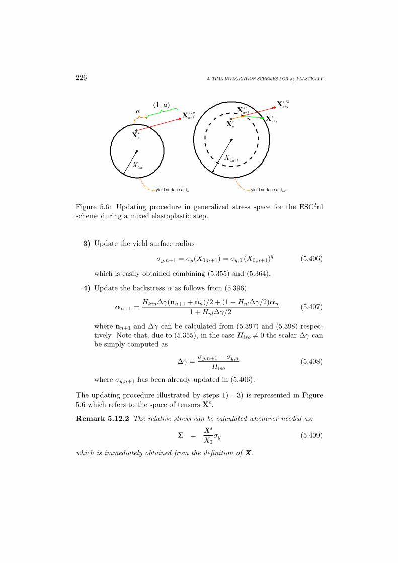
226 5. TIME-INTEGRATION SCHEMES FOR J2 PLASTICITY
Figure 5.6: Updating procedure in generalized stress space for the ESC2nlscheme during a mixed elastoplastic step.
3) Update the yield surface radius
σy,n+1 = σy(X0,n+1) = σy,0 (X0,n+1)q (5.406)
which is easily obtained combining (5.355) and (5.364).
4) Update the backstress α as follows from (5.396)
αn+1 =Hkin∆γ(nn+1 + nn)/2 + (1−Hnl∆γ/2)αn
1 +Hnl∆γ/2(5.407)
where nn+1 and ∆γ can be calculated from (5.397) and (5.398) respec-tively. Note that, due to (5.355), in the case Hiso = 0 the scalar ∆γ canbe simply computed as
∆γ =σy,n+1 − σy,n
Hiso(5.408)
where σy,n+1 has been already updated in (5.406).
The updating procedure illustrated by steps 1) - 3) is represented in Figure5.6 which refers to the space of tensors Xs.
Remark 5.12.2 The relative stress can be calculated whenever needed as:
Σ =Xs
X0σy (5.409)
which is immediately obtained from the definition of X.

5.12. ESC2NL EXPONENTIAL-BASED INTEGRATION SCHEME FOR THE NLK MODEL 227
Remark 5.12.3 The variable X0 is a local auxiliary variable and not an his-tory variable. In other words, introducing an appropriate scaling of the coupleX the variable X0 does not need to be updated at every time step [8].
Remark 5.12.4 The scalar α in the ESC2nl scheme is not to be confused withthe α parameter of the midpoint method presented in this same contribution.The author preferred to avoid renaming variables which already appear in theexisting literature.
5.12.4 ESC2nl scheme elastoplastic consistent tangent opera-tor
The algorithmically consistent tangent operator can be obtained properly lin-earizing the time-discrete procedure. To make notation more clear, the sub-scripts of all history variables evaluated at the end of the time interval tn+1 areomitted for brevity. Quantities evaluated either at tn or at tn+α are specifiedby the relative subscript.
For the total stress, from (5.343) and (5.313) it immediately follows
Cep =
∂σ
∂ε=[∂Σ∂e
+∂α
∂e
]Idev +K (I⊗ I) (5.410)
Then, a few calculations give
∂Σ∂e
=σy
X0
(∂Xs
∂e− 1− q
X0Xs∂X0
∂e
)(5.411)
while a direct derivation of the update procedure (5.407) gives∂α
∂e, which is
shown in the sequel.For the elastic phase we immediately have
∂Xs
∂e= 2GX0I (5.412)
∂X0
∂e= 0 (5.413)
while in the plastic phase the result is more complicated and is achieved asfollows. For the evaluation of the fourth-order tensors ∂X/∂e and ∂α/∂e, westart recalling that, for a general mixed elastoplastic step one has
Xs = Xs,en +
a− 1‖∆Ψ‖2
(∆Ψ : Xs,en )∆Ψ + b
X0,n
‖∆Ψ‖∆Ψ (5.414)

228 5. TIME-INTEGRATION SCHEMES FOR J2 PLASTICITY
where
Xs,en = Xs
n + α2Gσy,n
X0,n∆e (5.415)
a = cosh[(1− α)
2Gσy‖∆Ψ‖
](5.416)
b = sinh[(1− α)
2Gσy‖∆Ψ‖
](5.417)
∆Ψ = ∆Ψ0 + (1− α)∆Ψ1 (5.418)
Above, Xs,en represents the value of the second-order tensor Xs updated at
the end of the elastic part of the step. Moreover, ∆Ψ is the scaled drivingtensor, introduced to take into account that the plastic proportion of the stepamounts to (1− α)∆t.
The fourth-order tensor ∂Xs/∂e is obtained deriving expression (5.414).Without presenting all the calculations, it is found that
∂Xs
∂e= T1 + T2 + T3 (5.419)
In order to describe the three addenda T1, T2 and T3, a set of preliminaryderivatives is necessary.
Thus, we start introducing the second-order tensor υ = dα/d∆e
υ = φ1dCd∆e
+ φ2dDd∆e
φ1 =1D
(C√
C2 −DM− 1)
φ2 = − 1D2
(DM
2√C2 −DM
+√C2 −DM − C
)dCd∆e
= 2GX0,n Xsn
dDd∆e
= 2(2GX0,n)2∆e
(5.420)

5.12. ESC2NL EXPONENTIAL-BASED INTEGRATION SCHEME FOR THE NLK MODEL 229
Indeed, the following relations hold
∂∆Ψ∂e
=∂∆Ψ0
∂e+ (1− α)
∂∆Ψ1
∂e−∆Ψ1 ⊗ υ (5.421)
∂∆Ψ0
∂e= I +
q
X0,n(αn ⊗∆e) :
∂Xs,en
∂e+ q αn ⊗ ne (5.422)
+Hnl
Hiso(ne : ∆e) αn ⊗
∂q
∂e(5.423)
∂∆Ψ1
∂e=
12Hnl
2G
(∂Dα
∂eDγ + Dα⊗
∂Dγ
∂e+ αn ⊗
∂D′γ
∂e
)(5.424)
where
q =Hnl
Hisoq =
Hnl
2G1 −Hnl(ne : α)(5.425)
∂q
∂e=
HisoHnl
(2G1 −Hnl(ne : αn))2X−1
0,n
(∂Xs,e
n
∂e
)αn (5.426)
∂Dα
∂e= (Hkinne −Hnlαn)⊗ ∂Dγ
∂e+Hkin
Dγ
X0,n
∂Xs,en
∂e(5.427)
∂Dγ
∂e= (ne : ∆e)Φ + q
(ne +X−1
0,n
Xs,en
∂e∆e)
(5.428)
∂D′γ
∂e= T4 + T5 + T6 (5.429)
with ne = Xs,en /X0,n the normalized stress at the end of the elastic part. The
second-order tensors appearing in (5.428)-(5.429) are given by the followingexpressions
Φ = X−10,n
2GHnl
[2G1 −Hnl(ne : αn)]2∂Xs,e
n
∂eαn (5.430)
T4 = (ne : ∆e)Φ + q
(Dn +
∂Dn
∂e∆e)
(5.431)
T5 = Hnl [(Dn : α) + (ne : Dα)][
2(ne : ∆e)2G1 −Hnl(ne : αn)
Φ
+2G
[2G1 −Hnl(ne : αn)]2
(ne +X−1
0,n
∂Xs,en
∂e∆e)]
(5.432)
T6 =2GHnl
(2G1 −Hnl(ne : αn))2(ne : ∆e)
[∂Dn
∂∆eαn
+X−10,n
∂Xs,en
∂∆eDα +
∂Dα
∂∆ene
](5.433)

230 5. TIME-INTEGRATION SCHEMES FOR J2 PLASTICITY
with
∂Dn
∂∆e=
2Gσy,n
I− 2G1
σy,0
[DγX
−10,n
∂Xs,en
∂∆e+ ne ⊗
∂Dγ
∂∆e
](5.434)
+Hnl
σy,nαn ⊗
∂Dγ
∂∆e(5.435)
Let moreover
∂σy
∂e= σy,n
(log (1 + c)− c/(1 + c)
2 log 1 + c
)∂c
∂e(5.436)
where
∂c
∂e=
2Gqσy,n
[− (ne : ∆e)υ +
(1− α)X0,n
∂Xs,en
∂e∆e
+(1− α)ne +1− αq
(ne : ∆e)∂q
∂e
](5.437)
∂Xs,en
∂e= α
2Gσy,n
I +2Gσy,n
X0,n (∆e⊗ υ) (5.438)
Let in addition
∂‖∆Ψ‖∂e
=∂∆Ψ∂e
∆Ψ
‖∆Ψ‖(5.439)
∂
∂e
(∆Ψ
‖∆Ψ‖
)= ‖∆Ψ‖−2
(‖∆Ψ‖∂∆Ψ
∂e−∆Ψ⊗ ∂‖∆Ψ‖
∂e
)(5.440)
∂a
∂e= b
2Gσy
[−‖∆Ψ‖υ − (1− α)
‖∆Ψ‖σy
∂σy
∂e+ (1− α)
∂‖∆Ψ‖∂e
](5.441)
∂b
∂e= a
2Gσy
[−‖∆Ψ‖υ − (1− α)
‖∆Ψ‖σy
∂σy
∂e+ (1− α)
∂‖∆Ψ‖∂e
](5.442)

5.12. ESC2NL EXPONENTIAL-BASED INTEGRATION SCHEME FOR THE NLK MODEL 231
The fourth-order tensors defined in (5.419) are thus:
T1 =∂Xs,e
n
∂e+ α
2Gσy,n
X0,na− 1‖∆Ψ‖2
∆Ψ⊗∆Ψ
+ α2Gσy,n
X0,na− 1‖∆Ψ‖2
(∆Ψ : ∆e
)∆Ψ⊗ υ (5.443)
T2 =
(∆Ψ : Xs,e
n
)‖∆Ψ‖2
∆Ψ⊗ ∂a
∂e+
X0,n
‖∆Ψ‖∆Ψ⊗ ∂b
∂e(5.444)
T3 = (a− 1)
(∆Ψ
‖∆Ψ‖: Xs,e
n
)∂
∂e
(∆Ψ
‖∆Ψ‖
)
+ (a− 1)∆Ψ
‖∆Ψ‖⊗[∂
∂e
(∆Ψ
‖∆Ψ‖
)Xs,e
n
]
+bX0,n∂
∂e
(∆Ψ
‖∆Ψ‖
)(5.445)
The scalar function X0, following the algorithm of Section 5.12.2, is updatedas
X0 = b(∆Ψ : Xs,e
n )‖∆Ψ‖
+ aX0,n (5.446)
Therefore, a direct derivation gives
∂X0
∂e=
(∆Ψ : Xs,en )
‖∆Ψ‖∂b
∂e+
b
‖∆Ψ‖∂Xs,e
n
∂e∆Ψ + b
(∂
∂e∆Ψ
‖∆Ψ‖
)Xs,e
n +X0,n∂a
∂e(5.447)
which is readily calculated in view of the previous derivations in this section.
Finally, with respect to the derivative of the backstress α for an elastoplas-tic step, it holds
∂α
∂e=(Hkin
∂∆ep
∂e− 1
2Hnlαn ⊗
∂∆γ∂e
)(1 +
12Hnl∆γ
)−1
− Hnl
2
(1 +
12Hnl∆γ
)−2 [Hkin∆ep +
(1− 1
2Hnl∆γ
)αn
]⊗ ∂∆γ
∂e

232 5. TIME-INTEGRATION SCHEMES FOR J2 PLASTICITY
where
∆ep =12∆γ(
Xs
X0+
Xsn
X0,n
)(5.448)
∂∆γ∂e
=
qσy,0
HisoXq−1
0
∂X0
∂eif Hiso = 0
σy,0
2G1
X0,n
X0
∂X0
∂eif Hiso = 0
(5.449)
∂∆ep
∂e=
12∆γ
∂
∂e
(Xs
X0
)+
12
[(Xs
X0+
Xsn
X0,n
)⊗ ∂∆γ
∂e
](5.450)
∂
∂e
(Xs
X0
)=
1X0
∂Xs
∂e− 1X2
0
(Xs ⊗ ∂X0
∂e
)(5.451)
5.12.5 Brief review of the numerical properties of the ESC2nlmethod
The presented ESC2nl method satisfies the following algorithmical properties:
Yield consistency. As shown in (5.380), in the framework of formulation(5.376) the yield condition becomes
‖Xs‖2 = X20 (5.452)
at the end of all plastic steps. Following the same line of thought reported inSection 5.8.1, it can be immediately shown that such condition is fullfilled bythe ESC2nl scheme.
Second-order accuracy. Following standard calculations, namely a Taylorexpansion in time, it can be proved that the truncation error of the ESC2nlmethod is of order (∆t)2, where ∆t is the time step size. Therefore the schemeis second-order accurate, which guarantees a very reduced error at small timesteps.
Exactness in case of no hardening. If Hiso = Hnl = Hkin = 0, providede(t) is piecewise constant, the matrix in (5.376) is constant during each timestep. As a consequence, the evolution problem (5.376) is integrated exactly bythe exponential-based method presented. Therefore, whenever Hiso = Hnl =Hkin = 0, no error is introduced by the scheme in strain driven historieswith piecewise linear strain tensors. Although this property does not implyexactness in the general mixed stress-strain driven case, it is reflected in a verygood error behavior (see [10] for a brief discussion on this point).

5.12. ESC2NL EXPONENTIAL-BASED INTEGRATION SCHEME FOR THE NLK MODEL 233
Remark 5.12.5 Stability of the method is, from the theoretical viewpoint, stillto be addressed. This is for sure a point which should be further investigated.

234 5. TIME-INTEGRATION SCHEMES FOR J2 PLASTICITY

Chapter 6
Numerical tests
Introduzione
In questo capitolo vengono presentati alcuni test numerici relativi agli algoritmidi integrazione per modelli di plasticita J2 analizzati nel precedente Capitolo5. I test numerici hanno un duplice scopo. Il primo e quello di fornire un con-fronto in termini di precisione dei diversi schemi di integrazione considerati.Il secondo e quello di validare le proprieta numeriche dimostrate nel capitoloprecedente con riferimento particolare alla famiglia degli algoritmi di inte-grazione a base esponenziale. Le analisi summenzionate vengono sviluppateattraverso test numerici di tipo diverso. In particolare, si presentano i risul-tati inerenti storie di carico puntuali a controllo misto deformazioni-tensionie risultati relativi a problemi a valori iniziali e dati al bordo posti su continuitridimensionali.
Il capitolo e suddiviso in tre sezioni ed organizzato nel modo seguente.La Sezione 6.2 presenta il set-up delle diverse prove numeriche riportate nelcapitolo. Vengono qui introdotti i dettagli inerenti le strategie risolutive e diimplementazione algoritmica adottate, nonche le diverse misure d’errore uti-lizzate a seconda della prova considerata. La Sezione 6.3 riguarda il confrontonumerico degli algoritmi di integrazione del modello costitutivo J2 con incrudi-mento isotropo e cinematico lineare (modello LP). La Sezione 6.4 riguarda ilconfronto numerico degli algoritmi di integrazione del modello costitutivo J2
con incrudimento isotropo e cinematico lineare ed incrudimento cinematiconon lineare (modello NLK). Alcuni dei risultati presentati in questo capitolosono tratti da [6, 7, 8, 11, 12].
235

236 6. NUMERICAL TESTS
6.1 Introduction
In this chapter we present a set of numerical tests on the integration algorithmsfor J2 elastoplastic models analyzed in Chapter 5. The numerical tests havea double scope. First, they are intended to provide a comparison in terms ofprecision between the different considered integration schemes. On the otherhand, the numerical tests aim to validate the numerical properties and resultsfound in the previous chapter with particular emphasis to the exponential-based integration algorithms family. The above mentioned analyses are carriedout through different kinds of numerical tests. In particular, we present resultsrelative to pointwise mixed stress-strain loading histories and results relativeto initial boundary value problems on three-dimensional material bodies.
The chapter is divided in three sections and is organized as follows. Section6.2 is concerned with the setup of the numerical tests reported in the presentchapter. In this section the details inherent the solution strategies and thealgorithmic implementation adopted in the tests together with the differenterror measures are introduced. Section 6.3 is devoted to the comparison ofthe numerical schemes which apply to the J2 constitutive model with linearisotropic and kinematic hadening (LP model). Section 6.4 is devoted to thecomparison of the numerical schemes which apply to the J2 constitutive modelwith linear isotropic and kinematic hardening and nonlinear kinematic harden-ing (NLK model). Some of the results which are shown in this chapter aretaken from some works among which we cite [6, 7, 8, 11, 12].
6.2 Numerical tests setup
This section is devoted to the setup of the numerical tests presented in thefollowing sections. There are three different kinds of numerical tests. First, weconsider mixed stress-strain loading histories for a material point. The objectof this test is to study the accuracy granted by the method with respect tothe computation of the stress-strain asset. Second, we show a set of iso-error maps [69, 70] in order to evaluate the algorithm precision using differenttime discretizations. Finally, we present two classical initial boundary valueproblems, which we study to analyze the algorithm reliability on a practicalengineering problem.
As a result of the above numerical tests, we carry out a detailed comparisonof the presented methods in terms of precision, accuracy and in terms of specificproperties shown by each method. The pointwise tests and the iso-error mapsare performed with the aid of the CE-Driver code [15], the initial boundary

6.2. NUMERICAL TESTS SETUP 237
value problem is solved using FEAP [73]. Each test is described in detail asfollows.
6.2.1 Mixed stress-strain loading histories
We consider three biaxial non-proportional stress-strain loading histories de-fined on the reference time interval [0, T ], with T = 7 s. The consideredloading histories are obtained assuming to control two strain components andfour stress components, respectively, i.e.
Problem 1: ε11 σ22 σ33 ε12 σ13 σ23
Problem 2: ε11 ε22 σ33 σ12 σ13 σ23
Problem 3: ε11 σ22 σ33 ε12 σ13 σ23
For each history we require that all the controlled stress components are iden-tically equal to zero, while the strains are varied proportionally to
εy,mono =
√32σy,0
E(6.1)
which represents the first yielding strain value in a uniaxial loading history. Agraphical representation of the varying quantities is given in Figure 6.1.
Instantaneous error
Lacking the analytical solutions of the problems under investigation, we com-pute the “exact” solutions using a reference scheme (BE for the LP model,BEnl for the NLK model) with a very fine time discretization, correspondingto 100000 steps per second (∆t = 0.00001 s). The “exact” solutions are com-pared with the “numerical” ones, corresponding respectively to 10, 20 and 40steps per second (∆t = 0.1 s, 0.05 s, 0.025 s) and computed with each one ofthe compared algorithms.
The error is evaluated separately for the stress and the strain introducingthe following relative norms:
Eσn =
‖σn − σexn ‖
σy,nEεεε
n = 2G‖εεεn − εεεex
n ‖σy,n
(6.2)
where ‖ · ‖ indicates the usual euclidean norm and σy,n is the yield surfaceradius at time tn. In (6.2), σn and εεεn as well as σex
n and εεεexn are respectively
the stress and strain “numerical” and “exact” solution at time tn.

238 6. NUMERICAL TESTS
Pb. 1
Pb. 2
Pb. 3
Figure 6.1: Pointwise stress-strain tests. Mixed stress-strain loading historiesfor Problem 1, Problem 2 and Problem 3.

6.2. NUMERICAL TESTS SETUP 239
Figure 6.2: Plane stress von-Mises yield surface representation in principalstresses plane. State 1 choices for iso-error maps plots.
Total error
In order to further investigate the rate of convergence of the compared meth-ods, we also introduce the average total error as the 1 norm in time of theabsolute error:
EσT =
N∑n=1
∆tT
‖σn − σexn ‖
σy,nEεεε
T =N∑
n=1
2G∆tT
‖εεεn − εεεexn ‖
σy,n(6.3)
6.2.2 Iso-error maps
Iso-error maps are commonly adopted in the literature [51, 63, 64, 69] as asystematic tool to test the accuracy of plasticity integration algorithms. Inparticular, iso-error maps provide a clear evaluation of the integration algo-rithm accuracy when a large time discretization is adopted in solving particularpiecewise mixed stress-strain loading histories. Each loading history consid-ered in this chapter is set up by controlling the ε11 and ε22 strain componentsand requiring that all the remaining stresses are equal to zero. The evolutionin time of the controlled quantities is piecewise linear and can be divided intwo distinct phases defined as follows (see Table 6.1). Phase 1 consists of a

240 6. NUMERICAL TESTS
Table 6.1: Benchmark mixed stress-strain history for iso-error maps computa-tion.
Time [s] ε11 ε22 σ33 σ12 σ13 σ23
State 0 t=0 0 0 0 0 0 0State 1 t=1 ε11,y ε22,y 0 0 0 0State 2 t=2 εy,11 + ∆ε11 εy,22 + ∆ε22 0 0 0 0
Table 6.2: Iso-error maps. Choices for the State 1 point on the yield surface.
ε11,y ε22,y σ33 σ12 σ13 σ23
State 1-A εy,mono −νεy,mono 0 0 0 0
State 1-B (1− ν)εy,mono εy,mono 0 0 0 0
State 1-C(1 + ν)
3εy,mono −
(1 + ν)3
εy,mono 0 0 0 0
purely elastic path and proceeds from the zero stress and strain state (State0) to a specific state on the yield surface (State 1) given in terms of the yieldstrain components ε11,y and ε22,y. Phase 2 is a purely plastic path which startsfrom State 1 and leads to a final state (State 2) given in terms of the strainincrements ∆ε11 and ∆ε22.
In this analysis, we consider three different choices of State 1, correspond-ing to plane states of stress on the yield surface [69], labeled A, B and Crespectively, represented in Figure 6.2 and corresponding to uniaxial, biaxialand pure shear states. Each State 1 is expressed in Table 6.2 in terms of thequantity εy,mono (uniaxial yield strain) already defined in (6.1) according to
ε11 = ε11,y
ε22 = ε22,y
For each choice of State 1, we consider a State 2 defined as
ε11 = ε11,y + ∆ε11ε22 = ε22,y + ∆ε22
We solve a total of 60 × 60 mixed stress-strain histories for each State 1,corresponding to the following sets of normalized strain increments (see Figures

6.2. NUMERICAL TESTS SETUP 241
6.15-6.17 for instance)
∆ε11ε11,y
= 0.0, 0.1, 0.2, ..., 6.0
∆ε22ε22,y
= 0.0, 0.1, 0.2, ..., 6.0
This subdivision leads to a total of 3600 computed mixed stress-strain historiesand to an equal number of calculated relative error values. According to[69, 72], as an error measure, we adopt the following expression
Eσiso =
‖σ − σex‖‖σex‖ (6.4)
where σ is the final stress tensor, computed with a single time step discretiza-tion between State 1 and State 2, whereas σex corresponds to an “exact”solution adopting a very fine time step between State 1 and State 2.
6.2.3 Initial boundary value problems
We consider two three-dimensional thin rectangular perforated strips, sub-jected to uniaxial extension in a plane strain state [69]. The first strip has acircular hole in the center, while the second one has an elliptical hole. Bothstrips have three planes of symmetry and in Figure 6.4 we show one quarterof the domain for each of the two strips. The geometric lenghts referred toFigure 6.4 are
B = 100 mm H = 180 mm R0 = 50 mm H0 = 10 mm B0 = 50 mm
while the thickness is 10 mm.Initially the strip results undeformed and unstressed. The problem loading
history results symmetric with respect to the three symmetry planes of thestrip, hence we can refer to a single quarter of the domain and define thefollowing equivalent problem. The loading history, which is represented inFigure 6.3, is composed of a first phase (1 s), in which, the strip is stretchedassigning a top side vertical displacement δmax and a second phase (1 s) inwhich the imposed displacement is set back to 0 mm. We set δmax = 1 mm.We assume to block the horizontal displacement on the left side and to blockthe vertical displacement on the bottom side of the strip. The remainingboundary sides are stress free. In the analysis we consider Material 2 as donefor the iso-error map tests. We solve the boundary value problem using the

242 6. NUMERICAL TESTS
Figure 6.3: Initial boundary value problem. Loading history of imposed dis-placement on the top side of the strip and indication of L2 norm error plotinstants.
finite element code FEAP [73], in which the considered integration methodsare implemented. The mesh is composed of Nel finite elements (displacement-based four-node SOLID2D elements adopting a four point Gauss quadraturerule [73]). The following results refer to a mesh with Nel = 192 as can beobserved in Figure 6.5.
The comparison between the methods is carried out by evaluating thefollowing L2 norm error on stress and strain which makes use of stress andstrain output at Gauss quadrature points
Eσ =
√ ∫Ω ‖ σn − σex
n ‖2∫Ω ‖ σex
n ‖2≈
√√√√∑Neln=1
∑4q=1wnq ‖ σnq − σex
nq ‖2∑Neln=1
∑4q=1wnq ‖ σex
nq ‖2(6.5)
Eεεε =
√ ∫Ω ‖ εεεn − εεεex
n ‖2∫Ω ‖ εεεex
n ‖2≈
√√√√∑Neln=1
∑4q=1wnq ‖ εnq − εex
nq ‖2∑Neln=1
∑4q=1 wnq ‖ εex
nq ‖2(6.6)
In the above formulas, the indexes n and q respectively refer to the elementnumber and quadrature point number, while wnq is the qth quadrature pointGauss weight of the nth element. The quantities σnq and εεεnq are, respectively,the “numerical” stress and strain tensors calculated via the three integrationschemes adopting a prescribed time step ∆t, while σex
nq and εεεexnq are the corre-
sponding “exact” quantities evaluated with the reference scheme (BE for theLP model, BEnl for the NLK model) using an overkilling time step size. Inthe following tests we have chosen three different time steps sizes, respectively

6.2. NUMERICAL TESTS SETUP 243
Figure 6.4: Boundary value problems. Strips with circular and elliptical holes:geometry and imposed displacements for a single quarter of the strips.
∆t1 = 0.05 s, ∆t2 = 0.025 s, ∆t3 = 0.0125 s. The norms (6.5) and (6.6) areevaluated and plotted at four different instants (t = 0.5 s, t = 1.0 s, t = 1.5 s,t = 2.0 s) of the loading history (see Figure 6.3) with the three discretizationsdescribed above.
6.2.4 Material parameters
In the following analyses we consider five sets of material constants
• Material 1 [17]
E = 100 MPa ν = 0.3σy,0 = 15 MPa Hkin = 10 MPa Hiso = 10 MPaσy,0 = σy,0/E = 0.15 Hkin = Hkin/E = 0.1 Hiso = Hiso/E = 0.1
• Material 2 [69]
E = 30000 MPa ν = 0.3σy,0 = 3 MPa Hkin = 0 MPa Hiso = 0 MPaσy,0 = σy,0/E = 0.0001 Hkin = Hkin/E = 0 Hiso = Hiso/E = 0

244 6. NUMERICAL TESTS
Figure 6.5: Strips with circular and elliptical holes: plane projection of theadopted meshes
• Material 3 [79]
E = 7000 MPa ν = 0.3σy,0 = 24.3 MPa Hkin = 0 MPa Hiso = 225 MPaσy,0 = σy,0/E = 0.0034 Hkin = Hkin/E = 0 Hiso = Hiso/E = 0.032
• Material 4 [74]
E = 2× 10⁵ MPa ν = 0.3 σy,0 = 2× 10² MPaHiso = 0 MPa Hkin = 2× 10⁴ MPa Hnl = 50Hiso = Hiso/E = 0 Hkin = Hkin/E = 10−1 Hnl = Hnl/E = 2.5× 10⁻⁴
• Material 5 [74]
E = 2× 10⁵ MPa ν = 0.3 σy,0 = 2× 10² MPaHiso = 6× 10³ MPa Hkin = 2× 10⁴ MPa Hnl = 50Hiso = Hiso/E = 3× 10⁻² Hkin = Hkin/E = 10−1 Hnl = Hnl/E = 2.5× 10⁻⁴
Finally, we recall that the Young Modulus E and the Poisson ratio νuniquely determine the constants K and G as follows
K =E
3(1 − 2ν)G =
E
2(1 + ν)

6.3. NUMERICAL TESTS ON THE LP MODEL 245
6.3 Numerical tests on the LP model
In this section we present the numerical tests on the integration algorithmsdiscussed in Sections 5.3-5.7 which apply to the LP model. In what follows wesystematically adopt the following acronyms for the tested algorithms:
• BE Bacward Euler return map method (Section 5.3)• MPT Midpoint return map method (Section 5.4)• ENN Exp. Non-symm. Non-cons. method (Section 5.5)• ENC Exp. Non-symm. Cons. method (Section 5.6)• ESC Exp. Symm. Cons. method (Section 5.7)• ESC2 Exp. Symm. Cons. 2nd-order accurate method (Section 5.7)
6.3.1 Mixed stress-strain loading histories
The pointwise stress-strain tests are divided in two parts. First, we present aset of instantaneous error plots (Figures 6.6-6.9) corresponding to Problem 1and to Problem 2 solved with the first-order accurate BE and ESC meth-ods and with the exponential-based non-symmetric ENN and ENC meth-ods, respectively with Material 1 and Material 2. Then, in Figures 6.10-6.13, we present the corresponding instantaneous error plots obtained withthe quadratic methods MPT, ENC and ESC2. This splitting is done in orderto appreciate clearly the comparison in terms of precision between algorithmssharing the same order of accuracy.
From the error plots, we can extract the following comments
• The ESC and the BE methods perform similarly in terms of error, al-though in general the ESC seems slightly better. As the step size isreduced, both methods seem to converge with linear accuracy, i.e. theerror seems to be divided by 2 every time we double the number of steps(error goes as ∆t).
• The non symmetric methods ENN and ENC show practically the sameerror levels for all the considered stress-strain histories. These methodsperform decisively better than the ESC and BE algorithms. The orderof accuracy is 2 in this case and the error is roughly divided by 4 everytime we double the number of steps (error goes as (∆t)2).
• The performance of the MPT and the ENC methods are comparable.The MPT algorithm provides exact solutions for the case of proportionalloading. Finally, as the step size is reduced, both methods convergequadratically, i.e. the error is divided by 4 every time the number ofsteps is doubled (the error goes as ∆t2).

246 6. NUMERICAL TESTS
• The new symmetric method ESC2 grants relatively lower error levelsthan the MPT and ESC algorithms for all the considered stress-strainhistories. Also in this case, the numerical solution is exact for pro-portional loading conditions and the error decreases quadratically withrespect to the time step size.
We omit, for brevity’s sake, to provide the error plots regarding the remainingload histories since they would lead to conclusions similar to those given inthe above points.
Then, in Figure 6.14 we plot the total error expressed by Equation (6.3) ver-sus the number of time steps in logarithmic scale for the six methods BE, MPT,ENN, ENC, ESC and ESC2 for Problem 1 with Material 1. The quadratic con-vergence of the MPT, ENN, ENC and ESC2 methods with respect to the linearconvergence of the other algorithms can be clearly appreciated. It is remark-able that this error measurement qualifies the new optimal ESC2 scheme asthe most precise within the set of the tested algorithms, since it presents thelowest error levels both for the stress and the strain computation.
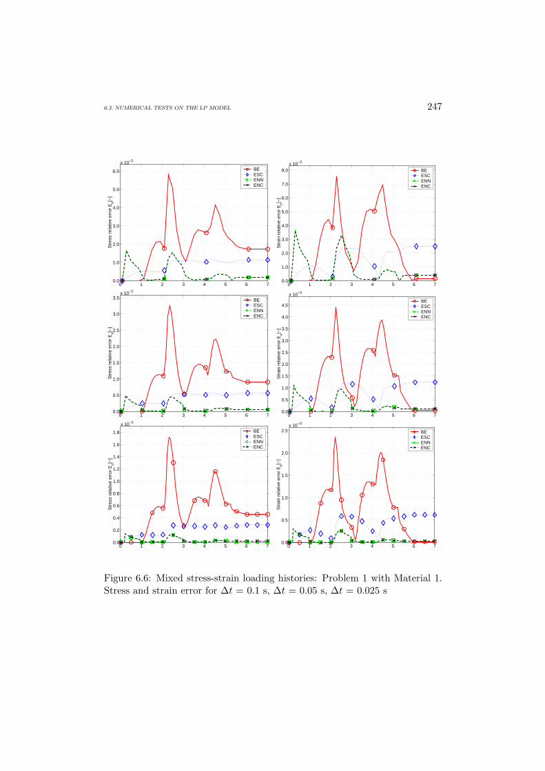
6.3. NUMERICAL TESTS ON THE LP MODEL 247
0 1 2 3 4 5 6 70.0
1.0
2.0
3.0
4.0
5.0
6.0
Str
ess
rela
tive
erro
r E
n[−]
BEESCENNENC
x 10−2
0 1 2 3 4 5 6 70.0
1.0
2.0
3.0
4.0
5.0
6.0
7.0
8.0
Str
ain
rela
tive
erro
r E
n[−]
BEESCENNENC
x 10−3
0 1 2 3 4 5 6 70.0
0.5
1.0
1.5
2.0
2.5
3.0
3.5
Str
ess
rela
tive
erro
r E
n[−]
BEESCENNENC
x 10−2
0 1 2 3 4 5 6 70.0
0.5
1.0
1.5
2.0
2.5
3.0
3.5
4.0
4.5
Str
ain
rela
tive
erro
r E
n[−]
BEESCENNENC
x 10−3
0 1 2 3 4 5 6 70.0
0.2
0.4
0.6
0.8
1.0
1.2
1.4
1.6
1.8
Str
ess
rela
tive
erro
r E
n[−]
BEESCENNENC
x 10−2
0 1 2 3 4 5 6 70.0
0.5
1.0
1.5
2.0
2.5
Str
ain
rela
tive
erro
r E
n[−]
BEESCENNENC
x 10−3
Figure 6.6: Mixed stress-strain loading histories: Problem 1 with Material 1.Stress and strain error for ∆t = 0.1 s, ∆t = 0.05 s, ∆t = 0.025 s

248 6. NUMERICAL TESTS
0 1 2 3 4 5 6 70.0
1.0
2.0
3.0
4.0
5.0
6.0
7.0
8.0
9.0
Str
ess
rela
tive
erro
r E
n[−]
BEESCENNENC
x 10−2
0 1 2 3 4 5 6 70.0
0.2
0.4
0.6
0.8
1.0
1.2
Str
ain
rela
tive
erro
r E
n[−]
BEESCENNENC
x 10−2
0 1 2 3 4 5 6 70.0
1.0
2.0
3.0
4.0
5.0
6.0
Str
ess
rela
tive
erro
r E
n[−]
BEESCENNENC
x 10−2
0 1 2 3 4 5 6 70.0
1.0
2.0
3.0
4.0
5.0
6.0
7.0
8.0
Str
ain
rela
tive
erro
r E
n[−]
BEESCENNENC
x 10−3
0 1 2 3 4 5 6 70.0
0.5
1.0
1.5
2.0
2.5
3.0
Str
ess
rela
tive
erro
r E
n[−]
BEESCENNENC
x 10−2
0 1 2 3 4 5 6 70.0
0.5
1.0
1.5
2.0
2.5
3.0
3.5
4.0
4.5
Str
ain
rela
tive
erro
r E
n[−]
BEESCENNENC
x 10−3
Figure 6.7: Mixed stress-strain loading histories: Problem 1 with Material 2.Stress and strain error for ∆t = 0.1 s, ∆t = 0.05 s, ∆t = 0.025 s

6.3. NUMERICAL TESTS ON THE LP MODEL 249
0 1 2 3 4 5 6 70.0
0.5
1.0
1.5
2.0
Str
ess
rela
tive
erro
r E
n[−]
BEESCENNENC
x 10−2
0 1 2 3 4 5 6 70.0
1.0
2.0
3.0
4.0
5.0
6.0
Str
ain
rela
tive
erro
r E
n[−]
BEESCENNENC
x 10−3
0 1 2 3 4 5 6 70.0
0.2
0.4
0.6
0.8
1.0
1.2
Str
ess
rela
tive
erro
r E
n[−]
BEESCENNENC
x 10−2
0 1 2 3 4 5 6 70.0
0.5
1.0
1.5
2.0
2.5
3.0
3.5
Str
ain
rela
tive
erro
r E
n[−]
BEESCENNENC
x 10−3
0 1 2 3 4 5 6 70.0
1.0
2.0
3.0
4.0
5.0
6.0
7.0
Str
ess
rela
tive
erro
r E
n[−]
BEESCENNENC
x 10−3
0 1 2 3 4 5 6 70.0
0.2
0.4
0.6
0.8
1.0
1.2
1.4
1.6
1.8
Str
ain
rela
tive
erro
r E
n[−]
BEESCENNENC
x 10−3
Figure 6.8: Mixed stress-strain loading histories: Problem 2 with Material 1.Stress and strain error for ∆t = 0.1 s, ∆t = 0.05 s, ∆t = 0.025 s

250 6. NUMERICAL TESTS
0 1 2 3 4 5 6 70.0
0.5
1.0
1.5
2.0
2.5
3.0
3.5
4.0
4.5
Str
ess
rela
tive
erro
r E
n[−]
BEESCENNENC
x 10−2
0 1 2 3 4 5 6 70.0
0.5
1.0
1.5
Str
ain
rela
tive
erro
r E
n[−]
BEESCENNENC
x 10−2
0 1 2 3 4 5 6 70.0
0.5
1.0
1.5
2.0
2.5
Str
ess
rela
tive
erro
r E
n[−]
BEESCENNENC
x 10−2
0 1 2 3 4 5 6 70.0
1.0
2.0
3.0
4.0
5.0
6.0
7.0
8.0
9.0
Str
ain
rela
tive
erro
r E
n[−]
BEESCENNENC
x 10−3
0 1 2 3 4 5 6 70.0
0.2
0.4
0.6
0.8
1.0
1.2
1.4
Str
ess
rela
tive
erro
r E
n[−]
BEESCENNENC
x 10−2
0 1 2 3 4 5 6 70.0
0.5
1.0
1.5
2.0
2.5
3.0
3.5
4.0
4.5
Str
ain
rela
tive
erro
r E
n[−]
BEESCENNENC
x 10−3
Figure 6.9: Mixed stress-strain loading histories: Problem 2 with Material 2.Stress and strain error for ∆t = 0.1 s, ∆t = 0.05 s, ∆t = 0.025 s
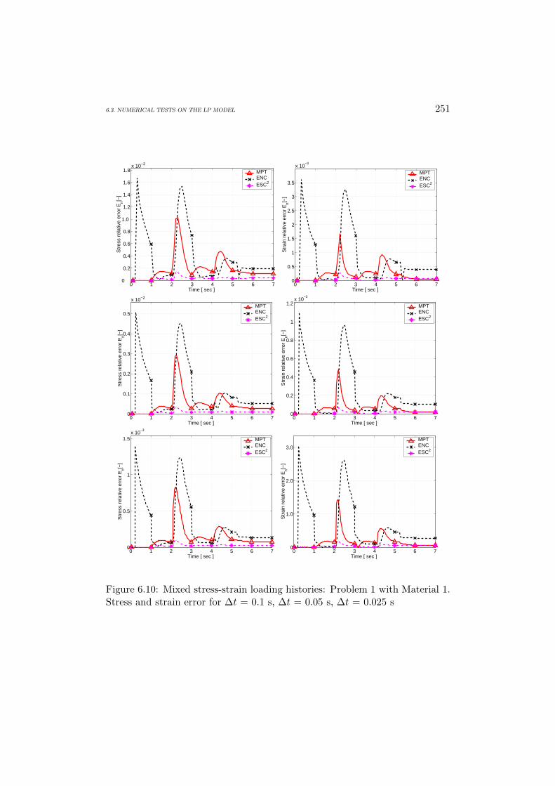
6.3. NUMERICAL TESTS ON THE LP MODEL 251
0 1 2 3 4 5 6 70
0.2
0.4
0.6
0.8
1.0
1.2
1.4
1.6
1.8
Time [ sec ]
Str
ess
rela
tive
erro
r E
n[−]
MPTENCESC2
x 10−2
0 1 2 3 4 5 6 70
0.5
1
1.5
2
2.5
3
3.5
x 10−3
Time [ sec ] S
trai
n re
lativ
e er
ror
En[−
]
MPTENCESC2
0 1 2 3 4 5 6 70
0.1
0.2
0.3
0.4
0.5
Time [ sec ]
Str
ess
rela
tive
erro
r E
n[−]
MPTENCESC2
x 10−2
0 1 2 3 4 5 6 70
0.2
0.4
0.6
0.8
1
1.2x 10
−3
Time [ sec ]
Str
ain
rela
tive
erro
r E
n[−]
MPTENCESC2
0 1 2 3 4 5 6 70
0.5
1
1.5x 10
−3
Time [ sec ]
Str
ess
rela
tive
erro
r E
n[−]
MPTENCESC2
0 1 2 3 4 5 6 70
1.0
2.0
3.0
Time [ sec ]
Str
ain
rela
tive
erro
r E
n[−]
MPTENCESC2
Figure 6.10: Mixed stress-strain loading histories: Problem 1 with Material 1.Stress and strain error for ∆t = 0.1 s, ∆t = 0.05 s, ∆t = 0.025 s

252 6. NUMERICAL TESTS
0 1 2 3 4 5 6 7
0.5
1
1.5
2
2.5
3
3.5
Time [ sec ]
Str
ess
rela
tive
erro
r E
n[−]
MPTENCESC2
x 10−2
00 1 2 3 4 5 6 7
0
1.0
2.0
3.0
4.0
5.0
6.0
Time [ sec ] S
trai
n re
lativ
e er
ror
En[−
]
MPTENCESC2
x 10−2
0 1 2 3 4 5 6 70
1.0
2.0
3.0
4.0
5.0
6.0
7.0
8.0
Time [ sec ]
Str
ess
rela
tive
erro
r E
n[−]
MPTENCESC2
x 10−3
0 1 2 3 4 5 6 70
0.2
0.4
0.6
0.8
1
1.2
x 10−3
Time [ sec ]
Str
ain
rela
tive
erro
r E
n[−]
MPTENCESC2
0 1 2 3 4 5 6 70
0.5
1
1.5
2
x 10−3
Time [ sec ]
Str
ess
rela
tive
erro
r E
n[−]
MPTENCESC2
0 1 2 3 4 5 6 70
0.5
1
1.5
2
2.5
3
3.5
x 10−4
Time [ sec ]
Str
ain
rela
tive
erro
r E
n[−]
MPTENCESC2
Figure 6.11: Mixed stress-strain loading histories: Problem 1 with Material 2.Stress and strain error for ∆t = 0.1 s, ∆t = 0.05 s, ∆t = 0.025 s

6.3. NUMERICAL TESTS ON THE LP MODEL 253
0 1 2 3 4 5 6 7
0.2
0.4
0.6
0.8
1
1.2
1.4
1.6
Time [ sec ]
Str
ess
rela
tive
erro
r E
n[−]
MPTENCESC2
x 10−2
00 1 2 3 4 5 6 7
0
1.0
2.0
3.0
4.0
5.0
6.0
Time [ sec ] S
trai
n re
lativ
e er
ror
En[−
]
MPTENCESC2
0 1 2 3 4 5 6 70
0.5
1
1.5
2
2.5
3
3.5
4
4.5
x 10−3
Time [ sec ]
Str
ess
rela
tive
erro
r E
n[−]
MPTENCESC2
0 1 2 3 4 5 6 70
0.2
0.4
0.6
0.8
1
1.2
1.4
1.6
x 10−3
Time [ sec ]
Str
ain
rela
tive
erro
r E
n[−]
MPTENCESC2
0 1 2 3 4 5 6 70
0.2
0.4
0.6
0.8
1
1.2
1.4x 10
−3
Time [ sec ]
Str
ess
rela
tive
erro
r E
n[−]
MPTENCESC2
0 1 2 3 4 5 6 70
0.5
1
1.5
2
2.5
3
3.5
4
4.5
5
x 10−4
Time [ sec ]
Str
ain
rela
tive
erro
r E
n[−]
MPTENCESC2
Figure 6.12: Mixed stress-strain loading histories: Problem 2 with Material 1.Stress and strain error for ∆t = 0.1 s, ∆t = 0.05 s, ∆t = 0.025 s

254 6. NUMERICAL TESTS
0 1 2 3 4 5 6 70
0.2
0.4
0.6
0.8
1.0
1.2
1.4
1.6
1.8
2.0
Time [ sec ]
Str
ess
rela
tive
erro
r E
n[−]
MPTENCESC2
x 10−2
0 1 2 3 4 5 6 70
1.0
2.0
3.0
4.0
5.0
6.0
7.0
Time [ sec ] S
trai
n re
lativ
e er
ror
En[−
]
MPTENCESC2
x 10−3
0 1 2 3 4 5 6 70
1.0
2.0
3.0
4.0
5.0
6.0
Time [ sec ]
Str
ess
rela
tive
erro
r E
n[−]
MPTENCESC2
x 10−3
0 1 2 3 4 5 6 70
0.5
1
1.5
2
x 10−3
Time [ sec ]
Str
ain
rela
tive
erro
r E
n[−]
MPTENCESC2
0 1 2 3 4 5 6 70
0.2
0.4
0.6
0.8
1
1.2
1.4
1.6
1.8x 10
−3
Time [ sec ]
Str
ess
rela
tive
erro
r E
n[−]
MPTENCESC2
0 1 2 3 4 5 6 70
1.0
2.0
3.0
4.0
5.0
6.0
7.0
Time [ sec ]
Str
ain
rela
tive
erro
r E
n[−]
MPTENCESC2
x 10−4
Figure 6.13: Mixed stress-strain loading histories: Problem 2 with Material 2.Stress and strain error for ∆t = 0.1 s, ∆t = 0.05 s, ∆t = 0.025 s

6.3. NUMERICAL TESTS ON THE LP MODEL 255
101
102
10−6
10−5
10−4
10−3
10−2
10−1
Steps/second
Str
ain
tota
l err
or E
[−]
BEMPTENNENCESCESC2
2
1
11
101
102
10−3
10−2
10−1
100
101
102
Steps/second
Str
ess
tota
l err
or E
[−]
BEMPTENNENCESCESC2
2
1
11
Figure 6.14: Pointwise stress-strain tests. Problem 1 with Material 1. Stressand strain total error versus number of steps per second.
6.3.2 Iso-error maps
In this section we present the iso-error maps corresponding to the three initialState 1 on the yield surface (cf. Table 6.2) and compare the precision levelsgranted by the BE, MPT and ESC2 integration algorithms, respectively. Allthe calculations refer to Material 2.
The total error range is subdivided in ten equally spaced levels according towhich the iso-curves are drawn in Figures 6.15-6.17. Each iso-curve is indicatedby a proper error label while the thick continuous line represents the zero-levelerror stress-strain histories (i.e. proportional loading histories). For the sakeof completeness, aside from each map we also report the maximum error valuecomputed on the grid adopted for the computation of the iso-error map.
Observing Figures 6.15-6.17, we recognize that the ESC2 scheme producesmore precise solutions in terms of stresses if compared to the BE and MPTalgorithms. Even for “large” strain increments the new exponential-basedprocedure reveals low levels of error compared with the other two methods.Such a result seems to be rather interesting since it suggests robustness of theintegration scheme for practical application of the integration procedure in afinite element analysis of boundary value problems. It is also worth noting thatthe BE scheme, which has linear accuracy, is more precise than the quadraticMPT algorithm for large strain increments. In this sense the ESC2 methodturns out to be the most reliable within the three methods, since it is quadraticand mantains good behavior also for large time steps.

256 6. NUMERICAL TESTS
A further observation is that, although Hiso = 0, the exponential-basedalgorithm presents a non zero error. This apparently erroneous behavior isdue to the fact that we have assumed a mixed stress-strain history and not acompletely strain driven one (see Reference [11] for a deeper discussion of thispoint).
Remark 6.3.1 It is noted that even with a non zero value of isotropic harden-ing the ESC2 scheme still produces more precise results for large time dis-cretizations than both the BE and MPT scheme. The reader is referred to [7]where a wide set of iso-error maps regarding this particular case confirm thebetter performance of the exponential-based method.
6.3.3 Initial boundary value problems
In this section we report the L2 norm error (6.5)-(6.6) obtained with theBE, ENC, ESC, MPT and ESC2 integration algorithms, respectively, for thesolution of the initial boundary value problems presented in Section 6.2.3. Theresults are summarized in Table 6.3 and Table 6.4 which report the norm errorat different instants during the loading history for the tested algorithms.
As expected, Table 6.3 and Table 6.4 show that the BE, ENC and ESCalgorithms grant first-order accuracy while the MPT and ESC2 are second-order accurate schemes. The tests indicate that the quadratic algorithms arefar more precise than the linear ones, both for the stress and the strain com-putation. The quadratically accurate ESC2 algorithm results globally moreprecise than the MPT.

6.3. NUMERICAL TESTS ON THE LP MODEL 257
BE
0 1 2 3 4 5 60
1
2
3
4
5
6
∆ε11
/ε11,y
∆ε22
/ε22
,y
2.99
5.99
8.99
11.99
14.99
17.99
20.99
2.99 5.99
Eσiso,max = 23.99%
MPT
0 1 2 3 4 5 60
1
2
3
4
5
6
∆ε11
/ε11,y
∆ε22
/ε22
,y
10.11
7.58
5.05
2.52
2.52
5.05
7.58
10.1112.64
15.17
17.7
Eσiso,max = 20.22%
ESC2
0 1 2 3 4 5 60
1
2
3
4
5
6
∆ε11
/ε11,y
∆ε22
/ε22
,y
3.18
2.72
2.27
1.81
1.36
0.9
0.45 0.45 0.9 1.36
Eσiso,max = 3.63%
Figure 6.15: Comparison between backward Euler (BE), midpoint (MPT)and the new exponential-based scheme (ESC2). Iso-error maps for yield sur-face State 1 - A with Material 2 and indication of the maximum stress errorlevel.

258 6. NUMERICAL TESTS
BE
0 1 2 3 4 5 60
1
2
3
4
5
6
∆ε11
/ε11,y
∆ε22
/ε22
,y
0.891.792.69
3.594.49
5.39
6.29
6.295.39
4.493.59
2.69
1.79
0.89
Eσiso,max = 7.18%
MPT
0 1 2 3 4 5 60
1
2
3
4
5
6
∆ε11
/ε11,y
∆ε22
/ε22
,y
17.23
14.77
12.31
9.84
7.38
4.92
2.46 2.46
4.92
7.38
9.8412.31
14.7717.23
Eσiso,max = 19.69%
ESC2
0 1 2 3 4 5 60
1
2
3
4
5
6
∆ε11
/ε11,y
∆ε22
/ε22
,y
0.36
0.310.26
0.20.15
0.1
0.05
0.05 0.1 0.15 0.2 0.260.310.36
Eσiso,max = 0.41%
Figure 6.16: Comparison between backward Euler (BE), midpoint (MPT)and the new exponential-based scheme (ESC2). Iso-error maps for yield sur-face State 1 - B with Material 2 and indication of the maximum stress errorlevel.

6.3. NUMERICAL TESTS ON THE LP MODEL 259
BE
0 1 2 3 4 5 60
1
2
3
4
5
6
∆ε11
/ε11,y
∆ε22
/ε22
,y 17.56
15.36 13.17
10.97
8.78
6.58
4.39
2.19
2.19
4.39
6.588.78
10.9713.17
15.36
17.56
Eσiso,max = 19.74%
MPT
0 1 2 3 4 5 60
1
2
3
4
5
6
∆ε11
/ε11,y
∆ε22
/ε22
,y
26.85
23.01
19.18
15.34
11.5
7.67
3.83
3.837.67
11.515.34
19.1823.01
26.85
Eσiso,max = 30.69%
ESC2
0 1 2 3 4 5 60
1
2
3
4
5
6
∆ε11
/ε11,y
∆ε22
/ε22
,y
4.55
3.98
3.41
2.84
2.27
1.71.13
0.56
0.561.131.72.272.84
3.413.98
4.55
Eσiso,max = 5.12%
Figure 6.17: Comparison between backward Euler (BE), midpoint (MPT)and the new exponential-based scheme (ESC2). Iso-error maps for yield sur-face State 1 - C with material 2 and indication of the maximum stress errorlevel.

260 6. NUMERICAL TESTS
Table 6.3: Initial boundary value problems. Extension of rectangular stripwith circular hole. Stress and strain L2 norm errors with Material 3 at t = 0.5s,t = 1.0 s,t = 1.5 s,t = 2.0 s for BE, ENC, ESC, MPT and ESC2 schemes
E ∆t BE ENC ESC MPT ESC2
t = 0.5 s∆t1 1.81×10⁻³ 1.15×10⁻³ 1.18×10⁻⁴ 1.36×10⁻⁴ 1.03×10⁻⁴
Eσ ∆t2 9.62×10⁻⁴ 3.26×10⁻⁴ 5.12×10⁻⁵ 3.24×10⁻⁵ 2.67×10⁻⁵
∆t3 4.96×10⁻⁴ 9.09×10⁻⁵ 2.76×10⁻⁵ 9.27×10⁻⁶ 7.11×10⁻⁶
∆t1 2.31×10⁻³ 2.08×10⁻³ 2.80×10⁻⁴ 3.02×10⁻⁴ 9.92×10⁻⁵
Eεεε ∆t2 1.24×10⁻³ 5.91×10⁻⁴ 1.20×10⁻⁴ 7.44×10⁻⁵ 2.12×10⁻⁵
∆t3 6.42×10⁻⁴ 1.62×10⁻⁴ 6.42×10⁻⁵ 2.31×10⁻⁵ 8.90×10⁻⁶
t = 1.0 s∆t1 3.07×10⁻³ 1.94×10⁻³ 6.32×10⁻⁴ 1.26×10⁻⁴ 1.11×10⁻⁴
Eσ ∆t2 1.58×10⁻³ 5.17×10⁻⁴ 3.13×10⁻⁴ 3.05×10⁻⁵ 2.55×10⁻⁵
∆t3 8.00×10⁻⁴ 1.32×10⁻⁴ 1.56×10⁻⁴ 7.81×10⁻⁶ 6.58×10⁻⁶
∆t1 2.57×10⁻³ 2.99×10⁻³ 1.40×10⁻³ 2.86×10⁻⁴ 2.96×10⁻⁴
Eεεε ∆t2 1.29×10⁻³ 8.12×10⁻⁴ 6.69×10⁻⁴ 5.87×10⁻⁵ 6.22×10⁻⁵
∆t3 6.53×10⁻⁴ 2.03×10⁻⁴ 3.30×10⁻⁴ 1.64×10⁻⁵ 1.69×10⁻⁵
t = 1.5 s∆t1 9.61×10⁻³ 6.10×10⁻³ 1.94×10⁻³ 2.31×10⁻¹ 3.61×10⁻⁴
Eσ ∆t2 1.14×10⁻¹ 1.14×10⁻¹ 1.16×10⁻¹ 1.15×10⁻¹ 1.15×10⁻¹
∆t3 5.72×10⁻² 5.74×10⁻² 5.81×10⁻² 5.78×10⁻² 5.78×10⁻²
∆t1 3.64×10⁻³ 4.23×10⁻³ 1.98×10⁻³ 5.23×10⁻² 4.19×10⁻⁴
Eεεε ∆t2 2.61×10⁻² 2.63×10⁻² 2.61×10⁻² 2.61×10⁻² 2.61×10⁻²
∆t3 1.30×10⁻² 1.31×10⁻² 1.30×10⁻² 1.30×10⁻² 1.30×10⁻²
t = 2.0 s∆t1 6.46×10⁻³ 3.40×10⁻³ 1.14×10⁻³ 2.92×10⁻⁴ 2.20×10⁻⁴
Eσ ∆t2 3.35×10⁻³ 9.06×10⁻⁴ 5.68×10⁻⁴ 6.98×10⁻⁵ 5.05×10⁻⁵
∆t3 1.70×10⁻³ 2.31×10⁻⁴ 2.83×10⁻⁴ 1.78×10⁻⁵ 1.28×10⁻⁵
∆t1 6.38×10⁻³ 5.64×10⁻³ 2.31×10⁻³ 5.27×10⁻⁴ 6.16×10⁻⁴
Eεεε ∆t2 3.24×10⁻³ 1.51×10⁻³ 1.12×10⁻³ 1.07×10⁻⁴ 1.30×10⁻⁴
∆t3 1.63×10⁻³ 3.79×10⁻⁴ 5.56×10⁻⁴ 2.98×10⁻⁵ 3.46×10⁻⁵
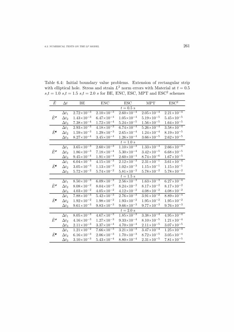
6.3. NUMERICAL TESTS ON THE LP MODEL 261
Table 6.4: Initial boundary value problems. Extension of rectangular stripwith elliptical hole. Stress and strain L2 norm errors with Material at t = 0.5s,t = 1.0 s,t = 1.5 s,t = 2.0 s for BE, ENC, ESC, MPT and ESC2 schemes
E ∆t BE ENC ESC MPT ESC2
t = 0.5 s∆t1 2.72×10⁻³ 2.10×10⁻³ 2.60×10⁻⁴ 2.05×10⁻⁴ 2.21×10⁻⁴
Eσ ∆t2 1.43×10⁻³ 6.47×10⁻⁴ 1.05×10⁻⁴ 5.19×10⁻⁵ 5.45×10⁻⁵
∆t3 7.38×10⁻⁴ 1.72×10⁻⁴ 5.24×10⁻⁵ 1.56×10⁻⁵ 1.64×10⁻⁵
∆t1 2.93×10⁻³ 4.18×10⁻³ 6.74×10⁻⁴ 5.26×10⁻⁴ 3.58×10⁻⁴
Eεεε ∆t2 1.59×10⁻³ 1.29×10⁻³ 2.65×10⁻⁴ 1.24×10⁻⁴ 8.19×10⁻⁵
∆t3 8.27×10⁻⁴ 3.45×10⁻⁴ 1.26×10⁻⁴ 3.66×10⁻⁵ 2.62×10⁻⁵
t = 1.0 s∆t1 3.65×10⁻³ 2.60×10⁻³ 1.10×10⁻³ 1.33×10⁻⁴ 2.66×10⁻⁴
Eσ ∆t2 1.86×10⁻³ 7.18×10⁻⁴ 5.30×10⁻⁴ 3.42×10⁻⁵ 6.68×10⁻⁵
∆t3 9.45×10⁻⁴ 1.91×10⁻⁴ 2.60×10⁻⁴ 8.74×10⁻⁶ 1.67×10⁻⁵
∆t1 6.04×10⁻³ 4.15×10⁻³ 2.12×10⁻³ 2.31×10⁻¹ 3.61×10⁻⁴
Eεεε ∆t2 3.05×10⁻³ 1.13×10⁻³ 1.02×10⁻³ 1.15×10⁻¹ 1.15×10⁻¹
∆t3 5.72×10⁻² 5.74×10⁻² 5.81×10⁻² 5.78×10⁻² 5.78×10⁻²
t = 1.5 s∆t1 8.50×10⁻³ 6.09×10⁻³ 2.56×10⁻³ 1.63×10⁻³ 6.27×10⁻⁴
Eσ ∆t2 8.08×10⁻² 8.04×10⁻² 8.24×10⁻² 8.17×10⁻² 8.17×10⁻²
∆t3 4.03×10⁻² 4.05×10⁻² 4.12×10⁻² 4.08×10⁻² 4.08×10⁻²
∆t1 7.88×10⁻³ 5.42×10⁻³ 2.76×10⁻³ 3.91×10⁻² 8.89×10⁻⁴
Eεεε ∆t2 1.92×10⁻² 1.98×10⁻² 1.93×10⁻² 1.95×10⁻² 1.95×10⁻²
∆t3 9.61×10⁻³ 9.83×10⁻³ 9.66×10⁻³ 9.77×10⁻³ 9.76×10⁻³
t = 2.0 s∆t1 8.05×10⁻³ 4.67×10⁻³ 1.85×10⁻³ 3.38×10⁻⁴ 4.95×10⁻⁴
Eσ ∆t2 4.16×10⁻³ 1.27×10⁻³ 9.33×10⁻⁴ 8.10×10⁻⁵ 1.21×10⁻⁴
∆t3 2.11×10⁻³ 3.37×10⁻⁴ 4.70×10⁻⁴ 2.11×10⁻⁵ 3.07×10⁻⁵
∆t1 1.21×10⁻² 7.66×10⁻³ 3.21×10⁻³ 3.47×10⁻⁴ 1.25×10⁻³
Eεεε ∆t2 6.16×10⁻³ 2.06×10⁻³ 1.70×10⁻³ 8.72×10⁻⁵ 3.05×10⁻⁴
∆t3 3.10×10⁻³ 5.43×10⁻⁴ 8.80×10⁻⁴ 2.31×10⁻⁵ 7.81×10⁻⁵

262 6. NUMERICAL TESTS
6.4 Numerical tests on the NLK model
In this section we present the numerical tests on the integration algorithmsdiscussed in Sections 5.10-5.12 which apply to the NLK model. In what followswe systematically adopt the following acronyms for the tested algorithms:
• BEnl Bacward Euler return map method (Section 5.10)• MPTnl Midpoint return map method (Section 5.11)• ESC2nl Exp. Symm. Cons. 2nd-order accurate method (Section 5.12)
6.4.1 Mixed stress-strain loading histories
The pointwise stress-strain tests are divided in two parts. First, we present aset of instantaneous error plots (Figures 6.18-6.21) corresponding to Problem 1and to Problem 2 solved with the BEnl, MPTnl and ESC2nl methods, respec-tively with Material 4 and Material 5. Then in Figures 6.22-6.25, we presentthe corresponding instantaneous error plots obtained with the quadratic meth-ods MPTnl and ESC2nl. This splitting is done in order to appreciate clearlythe comparison in terms of precision between the MPTnl and the ESC2nlalgorithm. It is evident from the presented error plots that
• The BEnl method is linearly accurate, that is the error is proportionalto the step size ∆t, while both the MPTnl and ESC2nl are quadraticallyaccurate, that is the error is proportional to the square of ∆t.
• The performance of the MPTnl and ESC2nl methods are globally com-parable. As the loading history evolves the exponential-based methodseems to produce lower error levels than the midpoint algorithm whenthere is a direction change in the driving input (the dashed line peaks onthe error plots are usually higher than the dash-dot line peaks). On theother hand, in most cases it is observed that the MPTnl algorithm errorlevels decrease more rapidly after the change of direction peaks than inthe case of the ESC2nl method.
• The two second-order accurate methods ESC2nl and MPTnl performdecisively better than the linearly accurate BEnl, for all the consideredstress-strain histories.
In Figure 6.26 we plot the total error expressed by (6.3) versus the num-ber of time steps in logarithmic scale for the three methods BEnl, MPTnl

6.4. NUMERICAL TESTS ON THE NLK MODEL 263
and ESC2nl for Problem 1 with Material 4. The quadratic convergenceof the MPTnl and ESC2nl methods, with respect to the linear one of theBEnl algorithm is still evident. Moreover, the quadratic methods showsignificantly lower error levels with respect to the ones granted by thelinear method. The ESC2nl method results more precise in stress com-putation than the MPT, while their strain error levels are practicallyequal.
6.4.2 Iso-error maps
In this section we present the iso-error maps corresponding to the three initialState 1 on the yield surface (cf. Table 6.2) and compare the precision levelsgranted by the BEnl, MPTnl and ESC2nl integration algorithms, respectively.All the calculations refer to Material 5.
The total error range is subdivided in ten equally spaced levels accordingto which the iso-curves are drawn in Figures 6.27-6.29. Each iso-curve isindicated by a proper error label while the thick continuous line representsthe couples of strain increments values corresponding to proportional loadinghistories starting from state 1. For the sake of completeness, aside from eachmap we also report the maximum error value computed on the grid adoptedfor the computation of the iso-error map. Observing Figures 6.27-6.29 we canderive the following conclusions
• the ESC2nl scheme shows better performances than both the BEnl andMPTnl algorithms for every considered starting yield State 1-A, 1-Band 1-C. Even for “large” strain increments the new exponential-basedprocedure reveals low levels of error compared with the other two meth-ods in all the examined cases.
• In general the BEnl scheme presents lower error levels for large strainincrements than the MPTnl method. This result is in agreement withthe general observation that lower order methods perform better thanhigher order ones for large time steps.
• None of the algorithms presents a zero error level along proportional load-ing paths (thick black lines, Figures 6.27-6.29). This is due to the factthat we have taken into account a nonlinear kinematic hardening mech-anism. However, in the vicinity of the thick black lines the exponential-based method seems to be more accurate than the other schemes.

264 6. NUMERICAL TESTS
0 1 2 3 4 5 6 70
1
2
3
4
5
6
7
Time [ sec ]
Str
ess
rela
tive
erro
r E
n[−]
BEnlMPTnlESC2nl
x 10−2
0 1 2 3 4 5 6 70
1
2
3
4
5
6
7
8
x 10−3
Time [ sec ] S
trai
n re
lativ
e er
ror
En[−
]
BEnlMPTnlESC2nl
0 1 2 3 4 5 6 70
0.5
1
1.5
2
2.5
3
3.5
4
Time [ sec ]
Str
ess
rela
tive
erro
r E
n[−]
BEnlMPTnlESC2nl
x 10−2
0 1 2 3 4 5 6 70
0.5
1
1.5
2
2.5
3
3.5
4
4.5
5x 10
−3
Time [ sec ]
Str
ain
rela
tive
erro
r E
n[−]
BEnlMPTnlESC2nl
0 1 2 3 4 5 6 70
0.5
1
1.5
2
Time [ sec ]
Str
ess
rela
tive
erro
r E
n[−]
BEnlMPTnlESC2nl
x 10−2
0 1 2 3 4 5 6 70
0.5
1
1.5
2
2.5
3x 10
−3
Time [ sec ]
Str
ain
rela
tive
erro
r E
n[−]
BEnlMPTnlESC2nl
Figure 6.18: Mixed stress-strain loading histories: Problem 1 with Material 4.Stress and strain error for ∆t = 0.1 s, ∆t = 0.05 s, ∆t = 0.025 s

6.4. NUMERICAL TESTS ON THE NLK MODEL 265
0 1 2 3 4 5 6 70
1
2
3
4
5
6
7
Time [ sec ]
Str
ess
rela
tive
erro
r E
n[−]
BEnlMPTnlESC2nl
x 10−2
0 1 2 3 4 5 6 70
1
2
3
4
5
6
7
8
9x 10
−3
Time [ sec ] S
trai
n re
lativ
e er
ror
En[−
]
BEnlMPTnlESC2nl
0 1 2 3 4 5 6 70
0.5
1
1.5
2
2.5
3
Time [ sec ]
Str
ess
rela
tive
erro
r E
n[−]
BEnlMPTnlESC2nl
x 10−2
0 1 2 3 4 5 6 70
0.5
1
1.5
2
2.5
3
3.5
4
4.5
x 10−3
Time [ sec ]
Str
ain
rela
tive
erro
r E
n[−]
BEnlMPTnlESC2nl
0 1 2 3 4 5 6 70
0.2
0.4
0.6
0.8
1
1.2
1.4
1.6
1.8
Time [ sec ]
Str
ess
rela
tive
erro
r E
n[−]
BEnlMPTnlESC2nl
x 10−2
0 1 2 3 4 5 6 70
0.5
1
1.5
2
2.5x 10
−3
Time [ sec ]
Str
ain
rela
tive
erro
r E
n[−]
BEnlMPTnlESC2nl
Figure 6.19: Mixed stress-strain loading histories: Problem 1 with Material 5.Stress and strain error for ∆t = 0.1 s, ∆t = 0.05 s, ∆t = 0.025 s

266 6. NUMERICAL TESTS
0 1 2 3 4 5 6 70
0.5
1
1.5
2
2.5
3
3.5
Time [ sec ]
Str
ess
rela
tive
erro
r E
n[−]
BEnlMPTnlESC2nl
x 10−2
0 1 2 3 4 5 6 70
0.1
0.2
0.3
0.4
0.5
0.6
0.7
0.8
0.9
1
Time [ sec ] S
trai
n re
lativ
e er
ror
En[−
]
BEnlMPTnlESC2nl
x 10−2
0 1 2 3 4 5 6 70
0.2
0.4
0.6
0.8
1
1.2
1.4
1.6
1.8
Time [ sec ]
Str
ess
rela
tive
erro
r E
n[−]
BEnlMPTnlESC2nl
x 10−2
0 1 2 3 4 5 6 70
1
2
3
4
5
6x 10
−3
Time [ sec ]
Str
ain
rela
tive
erro
r E
n[−]
BEnlMPTnlESC2nl
0 1 2 3 4 5 6 70
0.1
0.2
0.3
0.4
0.5
0.6
0.7
0.8
0.9
1
Time [ sec ]
Str
ess
rela
tive
erro
r E
n[−]
BEnlMPTnlESC2nl
x 10−2
0 1 2 3 4 5 6 70
0.5
1
1.5
2
2.5
3
x 10−3
Time [ sec ]
Str
ain
rela
tive
erro
r E
n[−]
BEnlMPTnlESC2nl
Figure 6.20: Mixed stress-strain loading histories: Problem 2 with Material 4.Stress and strain error for ∆t = 0.1 s, ∆t = 0.05 s, ∆t = 0.025 s
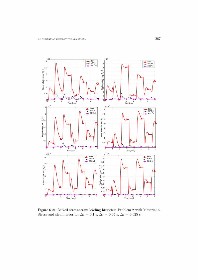
6.4. NUMERICAL TESTS ON THE NLK MODEL 267
0 1 2 3 4 5 6 70
0.5
1
1.5
2
2.5
3
Time [ sec ]
Str
ess
rela
tive
erro
r E
n[−]
BEnlMPTnlESC2nl
x 10−2
0 1 2 3 4 5 6 70
1
2
3
4
5
6
7
8
9
x 10−3
Time [ sec ] S
trai
n re
lativ
e er
ror
En[−
]
BEnlMPTnlESC2nl
0 1 2 3 4 5 6 70
0.2
0.4
0.6
0.8
1
1.2
Time [ sec ]
Str
ess
rela
tive
erro
r E
n[−]
BEnlMPTnlESC2nl
x 10−2
0 1 2 3 4 5 6 70
0.5
1
1.5
2
2.5
3
3.5
4
x 10−3
Time [ sec ]
Str
ain
rela
tive
erro
r E
n[−]
BEnlMPTnlESC2nl
0 1 2 3 4 5 6 70
1
2
3
4
5
6
x 10−3
Time [ sec ]
Str
ess
rela
tive
erro
r E
n[−]
BEnlMPTnlESC2nl
0 1 2 3 4 5 6 70
0.2
0.4
0.6
0.8
1
1.2
1.4
1.6
1.8
2
x 10−3
Time [ sec ]
Str
ain
rela
tive
erro
r E
n[−]
BEnlMPTnlESC2nl
Figure 6.21: Mixed stress-strain loading histories: Problem 2 with Material 5.Stress and strain error for ∆t = 0.1 s, ∆t = 0.05 s, ∆t = 0.025 s

268 6. NUMERICAL TESTS
0 1 2 3 4 5 6 70
0.5
1
1.5
2
2.5
3
3.5
Time [ sec ]
Str
ess
rela
tive
erro
r E
n[−]
MPTnlESC2nl
x 10−2
0 1 2 3 4 5 6 70
1
2
3
4
5
6
x 10−3
Time [ sec ] S
trai
n re
lativ
e er
ror
En[−
]
MPTnlESC2nl
0 1 2 3 4 5 6 70
1
2
3
4
5
6
7
x 10−3
Time [ sec ]
Str
ess
rela
tive
erro
r E
n[−]
MPTnlESC2nl
0 1 2 3 4 5 6 70
0.2
0.4
0.6
0.8
1
1.2
x 10−3
Time [ sec ]
Str
ain
rela
tive
erro
r E
n[−]
MPTnlESC2nl
0 1 2 3 4 5 6 70
0.2
0.4
0.6
0.8
1
1.2
1.4
1.6
1.8
x 10−3
Time [ sec ]
Str
ess
rela
tive
erro
r E
n[−]
MPTnlESC2nl
0 1 2 3 4 5 6 70.0
1.0
2.0
3.0
Time [ sec ]
Str
ain
rela
tive
erro
r E
n[−]
MPTnlESC2nl
x 10−4
Figure 6.22: Mixed stress-strain loading histories: Problem 1 with Material 4.Stress and strain error for ∆t = 0.1 s, ∆t = 0.05 s, ∆t = 0.025 s

6.4. NUMERICAL TESTS ON THE NLK MODEL 269
0 1 2 3 4 5 6 70
0.5
1
1.5
2
2.5
Time [ sec ]
Str
ess
rela
tive
erro
r E
n[−]
MPTnlESC2nl
x 10−2
0 1 2 3 4 5 6 70
0.5
1
1.5
2
2.5
3
3.5
4
4.5x 10
−3
Time [ sec ] S
trai
n re
lativ
e er
ror
En[−
]
MPTnlESC2nl
0 1 2 3 4 5 6 70
0.5
1
1.5
2
2.5
3
x 10−3
Time [ sec ]
Str
ess
rela
tive
erro
r E
n[−]
MPTnlESC2nl
0 1 2 3 4 5 6 70
0.5
1
1.5
2
2.5
3
3.5
4
4.5
5
x 10−4
Time [ sec ]
Str
ain
rela
tive
erro
r E
n[−]
MPTnlESC2nl
0 1 2 3 4 5 6 70
1
2
3
4
5
6
7
8
9
x 10−4
Time [ sec ]
Str
ess
rela
tive
erro
r E
n[−]
MPTnlESC2nl
0 1 2 3 4 5 6 70
0.5
1
1.5x 10
−4
Time [ sec ]
Str
ain
rela
tive
erro
r E
n[−]
MPTnlESC2nl
Figure 6.23: Mixed stress-strain loading histories: Problem 1 with Material 5.Stress and strain error for ∆t = 0.1 s, ∆t = 0.05 s, ∆t = 0.025 s

270 6. NUMERICAL TESTS
0 1 2 3 4 5 6 70
0.2
0.4
0.6
0.8
1
1.2
Time [ sec ]
Str
ess
rela
tive
erro
r E
n[−]
MPTnlESC2nl
x 10−2
0 1 2 3 4 5 6 70
0.5
1
1.5
2
2.5
3
3.5
4
4.5
x 10−3
Time [ sec ] S
trai
n re
lativ
e er
ror
En[−
]
MPTnlESC2nl
0 1 2 3 4 5 6 70
0.5
1
1.5
2
x 10−3
Time [ sec ]
Str
ess
rela
tive
erro
r E
n[−]
MPTnlESC2nl
0 1 2 3 4 5 6 70
1
2
3
4
5
6
7
8
x 10−4
Time [ sec ]
Str
ain
rela
tive
erro
r E
n[−]
MPTnlESC2nl
0 1 2 3 4 5 6 70
1
2
3
4
5
6
7
8x 10
−4
Time [ sec ]
Str
ess
rela
tive
erro
r E
n[−]
MPTnlESC2nl
0 1 2 3 4 5 6 70
1
2
3
x 10−4
Time [ sec ]
Str
ain
rela
tive
erro
r E
n[−]
MPTnlESC2nl
Figure 6.24: Mixed stress-strain loading histories: Problem 2 with Material 4.Stress and strain error for ∆t = 0.1 s, ∆t = 0.05 s, ∆t = 0.025 s

6.4. NUMERICAL TESTS ON THE NLK MODEL 271
0 1 2 3 4 5 6 70
1
2
3
4
5
6
x 10−3
Time [ sec ]
Str
ess
rela
tive
erro
r E
n[−]
MPTnlESC2nl
0 1 2 3 4 5 6 70
0.2
0.4
0.6
0.8
1
1.2
1.4
1.6
1.8
2x 10
−3
Time [ sec ]
Str
ain
rela
tive
erro
r E
n[−]
MPTnlESC2nl
0 1 2 3 4 5 6 70
0.2
0.4
0.6
0.8
1
1.2
x 10−3
Time [ sec ]
Str
ess
rela
tive
erro
r E
n[−]
MPTnlESC2nl
0 1 2 3 4 5 6 70
0.5
1
1.5
2
2.5
3
3.5
4
4.5
5
x 10−4
Time [ sec ]
Str
ain
rela
tive
erro
r E
n[−]
MPTnlESC2nl
0 1 2 3 4 5 6 70
1
2
x 10−4
Time [ sec ]
Str
ess
rela
tive
erro
r E
n[−]
MPTnlESC2nl
0 1 2 3 4 5 6 70
1
2
3
4
5
6
7
x 10−5
Time [ sec ]
Str
ain
rela
tive
erro
r E
n[−]
MPTnlESC2nl
Figure 6.25: Mixed stress-strain loading histories: Problem 2 with Material 5.Stress and strain error for ∆t = 0.1 s, ∆t = 0.05 s, ∆t = 0.025 s

272 6. NUMERICAL TESTS
101
102
10−1
100
101
102
103
104
Steps/second
Str
ess
tota
l err
or E
[−]
BEnlMPTnlESC2nl
1
1
1
2
101
102
10−8
10−6
10−4
10−2
100
Steps/second
Str
ain
tota
l err
or E
[−]
BEnlMPTnlESC2nl
1
2
1
1
Figure 6.26: Pointwise stress-strain tests. Problem 1 with Material 4. Stressand strain total error versus number of steps per second.
6.4.3 Initial boundary value problems
In this section we report the L2 norm error (6.5)-(6.6) obtained with the BEnl,MPTnl and ESC2nl integration algorithms, respectively, for the solution ofthe initial boundary value problems presented in Section 6.2.3. The resultsare summarized in Table 6.5 and Table 6.6, which report the norm error atdifferent instants during the loading history for the tested algorithms.
We may observe in Table 6.5 and Table 6.6 that the BEnl shows a first orderof accuracy while the MPTnl and ESC2nl are second-order accurate schemes.As shown in the tests, the quadratic algorithms are far more precise than thelinear one, both for the stress and the strain computation. The quadraticallyaccurate MPTnl and ESC2nl algorithms result globally comparable in termsof precision.
Summarizing, the midpoint and the exponential-based scheme seem tobehave very similarly. The higher peaks shown by the midpoint method inthe pointwise error graphs, seem to reveal a better behavior of the ESC2nlscheme whenever there is a crossing of the yield surface. Apart this difference,looking at the iso-error maps and the boundary value problem tests, it seemsthat the error behaviors of the two schemes are quite similar both for smalland large time step size.

6.4. NUMERICAL TESTS ON THE NLK MODEL 273
BEnl
0 1 2 3 4 5 60
1
2
3
4
5
6
∆ε11
/ε11,y
∆ε22
/ε22
,y
14.97
12.83
10.69
8.55
6.41
4.27
2.13
2.13
4.27
Eσiso,max = 17.11%
MPTnl
0 1 2 3 4 5 60
1
2
3
4
5
6
∆ε11
/ε11,y
∆ε22
/ε22
,y
8.857.596.32
5.06
3.79
2.53
1.26
1.262.53
3.79 5.06 6.32
7.59
Eσiso,max = 8.85%
ESC2nl
0 1 2 3 4 5 60
1
2
3
4
5
6
∆ε11
/ε11,y
∆ε22
/ε22
,y
4
3.2
2.4
1.6
0.8
0.8
1.62.4
3.24
4.8 5.6
Eσiso,max = 6.40%
Figure 6.27: Comparison between return map (BEnl), midpoint (MPTnl)and the new exponential-based scheme (ESC2nl). Iso-error maps for yieldsurface State 1 - A with Material 5 and indication of the maximum stresserror level.

274 6. NUMERICAL TESTS
BEnl
0 1 2 3 4 5 60
1
2
3
4
5
6
∆ε11
/ε11,y
∆ε22
/ε22
,y4.42
3.79
3.15
2.52
1.89
1.26
0.63
1.26
1.89 2.52
3.15
3.79
4.42
3.794.42
Eσiso,max = 4.42%
MPTnl
0 1 2 3 4 5 60
1
2
3
4
5
6
∆ε11
/ε11,y
∆ε22
/ε22
,y
7.996.85
5.74.56
3.422.28
1.14
1.14 2.28 3.42 4.56 5.76.85
7.99
Eσiso,max = 7.99%
ESC2nl
0 1 2 3 4 5 60
1
2
3
4
5
6
∆ε11
/ε11,y
∆ε22
/ε22
,y
3.482.98
2.481.99
1.490.99
0.49
0.49
0.99
1.49
1.992.48
2.983.48
Eσiso,max = 3.98%
Figure 6.28: Comparison between return map (BEnl), midpoint (MPTnl)and the new exponential-based scheme (ESC2nl). Iso-error maps for yieldsurface State 1 - B with Material 5 and indication of the maximum stresserror level.
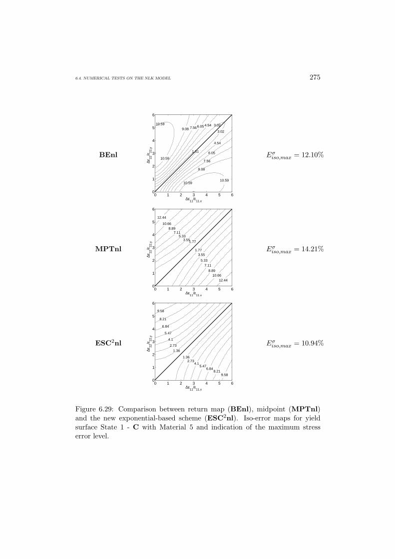
6.4. NUMERICAL TESTS ON THE NLK MODEL 275
BEnl
0 1 2 3 4 5 60
1
2
3
4
5
6
∆ε11
/ε11,y
∆ε22
/ε22
,y
10.59
10.59
9.08 7.566.05 4.54 3.02
3.02
1.51
4.54
6.05
7.56
9.08
10.5910.59
Eσiso,max = 12.10%
MPTnl
0 1 2 3 4 5 60
1
2
3
4
5
6
∆ε11
/ε11,y
∆ε22
/ε22
,y
12.44
10.668.89
7.115.33
3.551.77
1.773.55
5.337.11
8.8910.66
12.44
Eσiso,max = 14.21%
ESC2nl
0 1 2 3 4 5 60
1
2
3
4
5
6
∆ε11
/ε11,y
∆ε22
/ε22
,y
9.58
8.21
6.84
5.47
4.1
2.73
1.36
1.362.73
4.15.47
6.848.21
9.58
Eσiso,max = 10.94%
Figure 6.29: Comparison between return map (BEnl), midpoint (MPTnl)and the new exponential-based scheme (ESC2nl). Iso-error maps for yieldsurface State 1 - C with Material 5 and indication of the maximum stresserror level.

276 6. NUMERICAL TESTS
Table 6.5: Initial boundary value problems. Extension of rectangular stripwith circular hole. Stress and strain L2 norm errors with Material 5 at t = 0.5s,t = 1.0 s,t = 1.5 s,t = 2.0 s for BEnl, MPTnl and ESC2nl schemes.
E ∆t BEnl MPTnl ESC2nlt = 0.5
∆t1 4.41×10⁻³ 2.27×10⁻⁴ 3.95×10⁻⁴
Eσ ∆t2 2.27×10⁻³ 6.11×10⁻⁵ 1.04×10⁻⁴
∆t3 1.15×10⁻³ 1.61×10⁻⁵ 2.61×10⁻⁵
∆t1 3.72×10⁻³ 5.83×10⁻⁴ 6.44×10⁻⁴
Eε ∆t2 1.91×10⁻³ 1.52×10⁻⁴ 1.62×10⁻⁴
∆t3 9.65×10⁻⁴ 3.94×10⁻⁵ 4.15×10⁻⁵
t = 1.0∆t1 3.33×10⁻³ 6.87×10⁻⁵ 1.86×10⁻⁴
Eσ ∆t2 1.69×10⁻³ 1.84×10⁻⁵ 4.95×10⁻⁵
∆t3 8.48×10⁻⁴ 4.92×10⁻⁶ 1.25×10⁻⁵
∆t1 2.74×10⁻³ 1.97×10⁻⁴ 2.52×10⁻⁴
Eε ∆t2 1.40×10⁻³ 5.17×10⁻⁵ 6.34×10⁻⁵
∆t3 7.05×10⁻⁴ 1.32×10⁻⁵ 1.63×10⁻⁵
t = 1.5∆t1 1.48×10⁻² 1.62×10⁻³ 7.50×10⁻⁴
Eσ ∆t2 7.98×10⁻³ 4.42×10⁻⁴ 1.86×10⁻⁴
∆t3 4.17×10⁻³ 1.10×10⁻⁴ 4.51×10⁻⁵
∆t1 3.13×10⁻³ 2.21×10⁻⁴ 3.04×10⁻⁴
Eε ∆t2 1.54×10⁻³ 6.06×10⁻⁵ 7.08×10⁻⁵
∆t3 7.63×10⁻⁴ 1.40×10⁻⁵ 1.92×10⁻⁵
t = 2.0∆t1 5.05×10⁻³ 2.22×10⁻⁴ 2.14×10⁻⁴
Eσ ∆t2 2.57×10⁻³ 5.71×10⁻⁵ 5.15×10⁻⁵
∆t3 1.29×10⁻³ 1.48×10⁻⁵ 1.24×10⁻⁵
∆t1 8.08×10⁻³ 4.94×10⁻⁴ 9.74×10⁻⁴
Eε ∆t2 4.16×10⁻³ 1.13×10⁻⁴ 2.30×10⁻⁴
∆t3 2.10×10⁻³ 3.19×10⁻⁵ 6.45×10⁻⁵

6.4. NUMERICAL TESTS ON THE NLK MODEL 277
Table 6.6: Initial boundary value problems. Extension of rectangular stripwith elliptical hole. Stress and strain L2 norm errors with Material 5 at t = 0.5s,t = 1.0 s,t = 1.5 s,t = 2.0 s for BEnl, MPTnl and ESC2nl schemes.
E ∆t BEnl MPTnl ESC2nlt = 0.5
∆t1 4.48×10⁻³ 2.11×10⁻⁴ 7.10×10⁻⁴
Eσ ∆t2 2.30×10⁻³ 5.47×10⁻⁵ 1.83×10⁻⁴
∆t3 1.16×10⁻³ 1.47×10⁻⁵ 4.65×10⁻⁵
∆t1 5.56×10⁻³ 3.11×10⁻⁴ 1.44×10⁻³
Eε ∆t2 2.83×10⁻³ 8.00×10⁻⁵ 3.83×10⁻⁴
∆t3 1.42×10⁻³ 2.24×10⁻⁵ 9.76×10⁻⁵
t = 1.0∆t1 3.22×10⁻³ 6.73×10⁻⁵ 3.91×10⁻⁴
Eσ ∆t2 1.63×10⁻³ 1.68×10⁻⁵ 1.01×10⁻⁴
∆t3 8.22×10⁻⁴ 4.70×10⁻⁶ 2.59×10⁻⁵
∆t1 4.21×10⁻³ 1.27×10⁻⁴ 6.93×10⁻⁴
Eε ∆t2 2.13×10⁻³ 3.19×10⁻⁵ 1.82×10⁻⁴
∆t3 1.07×10⁻³ 8.81×10⁻⁶ 4.63×10⁻⁵
t = 1.5∆t1 1.21×10⁻² 1.22×10⁻³ 9.39×10⁻⁴
Eσ ∆t2 6.52×10⁻³ 3.26×10⁻⁴ 2.44×10⁻⁴
∆t3 3.39×10⁻³ 8.74×10⁻⁵ 6.15×10⁻⁵
∆t1 4.72×10⁻³ 2.00×10⁻⁴ 8.27×10⁻⁴
Eε ∆t2 2.34×10⁻³ 5.20×10⁻⁵ 2.24×10⁻⁴
∆t3 1.16×10⁻³ 1.46×10⁻⁵ 5.66×10⁻⁵
t = 2.0∆t1 5.22×10⁻³ 2.17×10⁻⁴ 3.71×10⁻⁴
Eσ ∆t2 2.66×10⁻³ 5.65×10⁻⁵ 9.65×10⁻⁵
∆t3 1.34×10⁻³ 1.50×10⁻⁵ 2.40×10⁻⁵
∆t1 9.58×10⁻³ 5.04×10⁻⁴ 2.30×10⁻³
Eε ∆t2 4.90×10⁻³ 1.31×10⁻⁴ 6.38×10⁻⁴
∆t3 2.46×10⁻³ 3.88×10⁻⁵ 1.62×10⁻⁴

278 6. NUMERICAL TESTS
Appendix A
Results from FunctionalAnalysis
A.1 Generalities
In what follows it is assumed that reader is familiar to the notions and theproperties of vector spaces. All vector spaces considered in the following willbe defined over the field of real numbers.
Normed spaces and Banach spaces
Let V be a vector space. A seminorm on V is a map | · | → R+ that issubadditive and positively homogenous, i.e. it satisfies the properties
|u+ v| ≤ |u|+ |v|, |αv| = |α| |v| ∀u, v ∈ V, ∀α ∈ R (A.1)
The above properties imply that |0| = 0 and |v| ≥ 0 for all v ∈ V . A norm‖ · ‖ on V is a special seminorm which is positive definite, i.e. it satisfies
‖ v ‖= 0 iff v = 0 (A.2)
If ‖ · ‖ is a norm on V , the pair (V, ‖ · ‖) is called a normed space. Commonly,a normed space (V, ‖ · ‖) is identified by the sole vector space V when thereis no confusion about the norm defined on it. The norm function ‖ · ‖ canbe interpreted as a generalization of the absolute value for the space of realnumbers and thus is seen as a measure of the length of a vector v ∈ V orequivalently of the distance between v and the null vector of V . Accordingly,the expression ‖ u− v ‖ returns the distance between two points u and v of V .
Two distinct norms ‖ · ‖1 and ‖ · ‖2 defined over the same space V are saidto be equivalent if there exist two strictly positive constants c1 and c2 such
279

280 A. RESULTS FROM FUNCTIONAL ANALYSIS
that
c1 ‖ v ‖1≤‖ v ‖2≤ c2 ‖ v ‖1 (A.3)
A well known property is that any two norms defined on a finite-dimensionalvector space are equivalent. By contrast, this is not true in an infinite-dimensional space. The above notions are recalled since in the analysis ofboundary value problems a common technique is that of establishing esti-mates using some norm equivalent to the conventional norm of the functionspace for the problem.
A sequence vn in a normed space V converges (strongly) to a vectorv ∈ V if and only if limn→∞ ‖ vn − v ‖= 0. This occurrence is indicated byvn → v or by saying that v is the (strong) limit of the sequence vn. Giventwo equivalent norms ‖ · ‖1 and ‖ · ‖2 defined over the space V , it can beshown that a sequence vn ⊂ V converges to a vector v ∈ V in the norm‖ · ‖1 if and only if it converges to v in the norm ‖ · ‖2.
A subset A of V is said to be closed in V if any converging sequence ofelements of A has its limit in A. The closure A of A is the smallest closed setof V containing A; in other words, we may say that A is obtained by addingto A its “boundary points”. The set A is dense in V if for every v ∈ V thereexists a sequence vn in A such that vn → v, or, equivalently, if A = V .The set A is said to be bounded if there exists a positve constant M such that‖ v ‖≤M for every v ∈ V .
A Cauchy sequence in V is a sequence vn of elements of V such that forany ε > 0, there exists an integer N(ε) such that, for all n and m larger thanN(ε), ‖ vn − vm ‖< ε. This property simply means that the elements of thesequence are restricted to an arbitrarily small region of the space, providedthat we consider elements of sufficiently high rank. Indeed, all convergentsequences are Cauchy sequences, while the converse is not true. A Banachspace A is a normed vector space which is complete, i.e. in which all Cauchysequences converge strongly to an element of the space. We have then thefollowing proposition that relates the properties of completeness and closednessin normed spaces.
Proposition A.1.1 A subset of a Banach space is complete if and only if itis closed.
Linear operators and linear functionals
Let V and W be vector spaces. Let L : V → W be a map from V to W , alsocalled an operator. The operator L is said to be linear if it is additive and

A.1. GENERALITIES 281
homogeneous, that is, if for all u, v ∈ V and α ∈ R, it holds
L(u+ v) = L(u) + L(v)L(αv) = αL(v)
Commonly the action of L on v is denoted with Lv instead of L(v). If thespace W coincides with R, then L is called a functional.
The range R(L) and the kernel or null space N (L) of L are subspaces ofW and V , defined respectively by
R(L) = w ∈W : w = L(v) for some v ∈ V N (L) = v ∈ V : L(v) = 0
meaning that R(L) represents the set of images under the mapping L, whilethe null space N (L) is given by the elements in V which are mapped to thezero element of W .
If V and W are normed vector spaces and L is a map from V into W , thenL is said to be continuous if to any converging sequence vn → v in V therecorresponds the converging sequence L(vn)→ L(v) in W . The map L is saidto be bounded if for any r > 0, there exists a constant R ≥ 0 such that
‖ L(v) ‖≤ R ∀v ∈ V, s.t. ‖ v ‖≤ r
Any linear bounded operator L is characterized by the properties that
‖ L(v) ‖≤M ‖ v ‖ ∀v ∈ V (A.4)
with M a nonnegative constant. It can be shown that a linear operator iscontinuous if and only if it is bounded.
Finally, the operator L will be said Lipschitz continuous if there exists aconstant c > 0 such that
‖ L(v1)− L(v2) ‖≤ c ‖ v1 − v2 ‖ ∀v1, v2 ∈ V
Lipschitz continuous operators are continuous, but the converse is not true ingeneral. On the other hand, a linear operator is Lipschitz continuous if andonly if it is continuous.
Bilinear forms
Given two vector spaces V and W , a map b : V ×W → R is called a bilinearform if it is linear in each slot, that is, if it satisfies the following properties
b(αv1 + βv2, w) = αb(v1, w) + βb(v2, w)b(v, αw1 + βw2) = αb(v,w1) + βb(v,w2)
282 A. RESULTS FROM FUNCTIONAL ANALYSIS
for any v1, v2, v ∈ V , w1, w2, w ∈W and α, β ∈ R.A bilinear form b : V ×W → R is said to be continuous if there exists a
positive constant M such that
b(v,w) ≤M ‖ v ‖V ‖ w ‖W ∀v ∈ V, ∀w ∈W
In the case where W = V , the bilinear form is symmetric if
b(v1, v2) = b(v2, v1) ∀v1, v2 ∈ V
while it is V-elliptic if there exists a constant α > 0 such that
b(v, v) ≥ α ‖ v ‖2 ∀v ∈ V
Isomorphisms and completions
A linear continuous map L : V → W which is both injective, i.e. one-to-oneand surjective, which means R(L) = W , is called an isomorphism.
Given a normed space V , its completion is a Banach space V , which holdsthe property that there exists an isomorphism from V onto a dense subspaceof V . A classical example in this sense is the completion of the continuousfunction space C([0, 1]) in the norm ‖ v ‖0= (
∫ 10 |v(x)|2dx)1/2 which coincides
with the Lebesgue space L2(0, 1) [41].
The space L(V,W ). Dual space
Let V and W be normed spaces. The space of all bounded linear operatorsfrom V to W is denoted by L(V,W ). The conventional or natural norm definedover the space L(V,W ) is
‖ L ‖L(V,W )= supv∈V \0
‖ Lv ‖W‖ v ‖V
= sup‖v‖V ≤1
‖ Lv ‖W (A.5)
which is always a well-defined quantity as can be deduced from (A.4). It canbe shown that the space L(V,W ) endowed with the norm (A.5) is a Banachspace if W is a Banach space.
The space L(V,R) of bounded linear functionals on V is defined as thedual space of V and is denoted by V ′. It follows that, since R is complete, V ′
is a Banach space with the norm
‖ L ‖V ′= sup‖v‖V ≤1
|Lv| (A.6)

A.1. GENERALITIES 283
In the following, the symbol will be frequently used to indicate a boundedlinear functional on a normed space V , while the image (v) of a vector v ∈ Vthrough , will be denoted by V ′〈, v〉V rather than l(v). The map 〈·, ·〉 :V ′×V →R is known as the duality pairing between V and V ′. Some examplesof duality will be addressed in Section A.2.1 in the context of the function spaceLp(Ω). In the following, when there is no amboguity, we simply indicate with〈·, ·〉 the duality pairing between V ′ and V .
Monotone and strongly monotone operators
An operator T : V → V ′ is said to be monotone if
〈T (u)− T (v), u − v〉 ≥ 0 ∀u, v ∈ V
and it is said to be strongly monotone if there exists a constant c > 0 suchthat
〈T (u)− T (v), u− v〉 ≥ c ‖ u− v ‖2 ∀u, v ∈ V
Biduals and reflexivity
The dual V ′ of a normed space V is a Banach space and V ′ itself has a dualV ′′ ≡ (V ′)′, called the bidual of V . Of course, the bidual is a Banach spaceand it is possible to show that there exists a bounded linear operator J fromV onto V ′′ that is one-to-one and also an isometry, i.e. ‖ Jv ‖=‖ v ‖,∀v ∈ V .It follows that V can be identified with a subspace J(V ) of V ′′. The normedspace V is said to be reflexive if the following identity holds
J(V ) = V ′′ (A.7)
To indicate the above relationship we briefly write V ′′ = V . Indeed, a reflexivenormed space is a Banach space. A classical example of a reflexive Banachspace is provided by the space Lp(Ω) (see Section A.2.1) for p ∈ (1,∞) inwhich Ω ⊂ Rd is an open set.
Weak convergence
Let V be a normed space and V ′ its dual. A sequence vn ⊂ V is said toconverge weakly in V to v if
limn→∞
〈, vn〉 = 〈, v〉 ∀ ∈ V ′ (A.8)

284 A. RESULTS FROM FUNCTIONAL ANALYSIS
The above notion is indicated by the following notation
vn v
It is noted that strong convergence implies weak convergence, while the con-verse is not true, with the only exception of finite-dimensional spaces for whichthe two kinds of convergence coincide.
Compactness and weak compactness
A subset V1 of a normed space V is said to be (sequentially) compact if everybounded sequence in V1 has a subsequence that converges in V1. Likewise,V1 is weakly compact if every bounded sequence in V1 has a subsequence thatconverges weakly in V1.
A linear operator L : V → W is said to be compact if the image under Lof a bounded sequence in V contains a subsequence converging in W , that is,if vn ⊂ V is bounded, then there exists a subsequence vnj and an elementw ∈W such that Lvnj → w inW . If in the above definition strong convergenceis replaced by weak convergence and Lvnj w in W , then L is said to beweakly compact. Clearly, L is compact if and only if it maps bounded sets tocompact sets. We have now the following important result
Theorem A.1.2 (Eberlein-Smulyan). A reflexive Banach space V is weaklycompact, that is, if vn is a bounded sequence of V , then it results possible toextract a subsequence of vn that converges weakly in V. If, furthermore, thelimit v is independent of the subsequence extracted, then the whole sequencevn converges weakly to v.
Embeddings
Let V and W be normed spaces with V ⊂W . If there is a constant c > 0 suchthat
‖ v ‖W≤ c ‖ v ‖V ∀v ∈ V (A.9)
we say that V is continuously embedded in W and write
V →W
The property (A.9) can be interpreted in various ways, for instance it allowsto state that the identity operator I : V → W is bounded or, equivalently,continuous. Moreover the continuous embedding of V into W implies that ifvn → v in V , then also vn → v in W .

A.1. GENERALITIES 285
A subspace V is said to be compactly embedded in W if
vn v in V implies vn → v in W
This property is expressed in the form
V →→ W
and is equivalent to the statement that the identity operator from V into Wis compact [41].
The above embedding results will be useful in the next section whenSobolev spaces with different indices are compared.
Dual operators
Consider a couple of normed spaces V and W and their respective dual spacesV ′ and W ′. Let A be a linear operator with domain D(A) ⊂ V and range inW . Given a vector w′ ∈W ′, it can be shown that there exists a vector v′ ∈ V ′
such that
W ′〈w′, Av〉W =V ′ 〈v′, v〉V ∀v ∈ D(A) (A.10)
if and only if D(A) is dense in V . If this is the case, then v′ is uniquelydetermined by w′. When D(A) coincides with V , then the above reasoningdefines a linear operator A′ from W ′ to V ′ such that A′w′ = v′. The operatorA′ is called the dual operator of A and is such that the following statementholds
W ′〈w′, Av〉W =V ′ 〈A′w′, v〉V ∀v ∈ V, ∀w′ ∈W ′
If D(A) = V and A is bounded, then A′ is also bounded and
‖ A′ ‖=‖ A ‖
We have now the following important theorem which illustrates furtherrelationships existing between dual operators.
Theorem A.1.3 (Closed Range Theorem). Let V and W be two Banachspaces and let A be a bounded linear operator from V to W with dual operatorA′. Then the following statements are equivalent:
• R(A) is closed in W
• R(A′) is closed in V ′

286 A. RESULTS FROM FUNCTIONAL ANALYSIS
• R(A) = [KerA′] ≡ w ∈W : 〈, w〉 = 0 ∀ ∈ KerA′
• R(A′) = [KerA] ≡ ∈ V ′ : 〈, v〉 = 0 ∀v ∈ KerAThe next result follows directly from the closed range theorem
Corollary A.1.4 The following results hold:
• R(A) = W iff there exists a constant c such that ‖ A′ ‖V ′≥ c1 ‖ ‖W ′
∀ ∈W ′
• R(A′) = V ′ iff there exists a constant c such that ‖ Av ‖W≥ c2 ‖ v ‖V∀v ∈ V
The Babuska-Brezzi condition for bilinear forms
Let b : V × W → R be a continuous bilinear form, that is there exists aconstant αb > 0 such that
|b(v,w)| ≤ αb ‖ v ‖V ‖ w ‖W ∀v ∈ V, ∀w ∈W (A.11)
The bilinear form b(·, ·) is said to satisfy the Babuska-Brezzi condition if thereexists a constant βb > 0 such that
supw∈W\0
|b(v,w)|‖ w ‖W
≥ βb ‖ v ‖V ∀v ∈ V (A.12)
The following theorem establishes the relationship between the Babuska-Brezzi condition and the closed range theorem [18, 22].
Theorem A.1.5 Let b : V ×W → R be a continuous bilinear form whichdefines bounded linear operators B : V → W ′ and B′ : W → V ′, according to
b(v,w) =W ′ 〈Bv,w〉W =V ′ 〈B′w, v〉V ∀v ∈ V, w ∈WWith the above hypotheses, the following statements are equivalent
• The bilinear form b(·, ·) satisfies the Babuska-Brezzi condition (A.12)
• The operator B is an isomorphism from (KerB) onto W ′, where
KerB = v ∈ V : b(v,w) = 0 ∀w ∈W
• The operator B′ is an isomorphism from W onto (KerB), where
(KerB) = ∈ V ′ : 〈, v〉 = 0 ∀v ∈ KerB
The Babuska-Brezzi condition is the crucial key-point in the analysis of mixedor saddle-point variational problems like those related to the formulation ofthe elastoplastic boundary value problem addressed in Chapter 3.

A.1. GENERALITIES 287
Inner products and Hilbert spaces
An inner product is a generalization of the ordinary vector scalar product inRd to an arbitrary vector space. Let V be a vector space. An inner producton V is a symmetric positive-definite bilinear form (·, ·) : V × V →R, namelysuch that
(u, v) = (v, u) ∀u, v ∈ V(αu1 + βu2, v) = α(u1, v) + β(u2, v) ∀u1, u2, v ∈ V, ∀α, β ∈ R
(v, v) ≥ 0 ∀v ∈ V, and (v, v) = 0⇔ v = 0
An inner product space is a vector space endowed with an inner product. Whenthe definition of the inner product (·, ·) is clear, we will briefly denote the innerproduct space with V .
From the definition above it follows immediately that any inner productspace is a normed space with the norm
‖ v ‖= (v, v)1/2
A complete inner product space is called a Hilbert space. It is evident that anyHilbert space is a Banach space with the norm induced by its inner product.
Consider now the following classical results on inner product and Hilbertspaces.
Theorem A.1.6 (Cauchy-Schwartz Inequality). Given an inner prod-uct space V , it holds
|(u, v)| ≤‖ u ‖‖ v ‖ ∀u, v ∈ V
Theorem A.1.7 (Riesz Representation Theorem). Any Hilbert spaceV can be identified with its dual V ′ by means of an isometric isomorphism.More precisely, for any ∈ V ′ there exists a unique u ∈ V such that
〈, v〉 = (u, v) ∀v ∈ V‖ ‖V ′ = ‖ u ‖V
On the other hand, for any u ∈ V , the mapping v → (u, v) determines anelement ∈ V ′ such that ‖ ‖V ′=‖ u ‖V
From the last theorem it follows immediately that a Hilbert space can beidentified with its bidual as well. Therefore, we have the following
Corollary A.1.8 Every Hilbert space is reflexive.

288 A. RESULTS FROM FUNCTIONAL ANALYSIS
Now combining the statements of Theorem A.1.7 and Corollary A.1.8 it isfound that in a Hilbert space every bounded sequence has a weakly convergentsubsequence. We have thus the property that on an inner product space V
vn v ⇒‖ v ‖≤ limn→∞
inf ‖ vn ‖
which can be equivalently stated by saying that the norm function ‖ · ‖ of aninner product space is weakly l.s.c. The last proposition can be proved simplyby checking that for a fixed w ∈ V , the mapping v → (w, v) defines a boundedand continuous functional on V and thus
‖ v ‖2= (v, v) = limn→∞
(v, vn) ≤‖ v ‖ limn→∞
inf ‖ vn ‖
The last property will be frequently used in Section 3.3.We now present a well-known fundamental result which comes into play in
proving the unique solvability of elliptic variational problems
Theorem A.1.9 (Lax-Milgram Lemma). Let V be a Hilbert space. Givena continuous and V-elliptic bilinear form b : V ×V → R and a bounded linearfunction : V →R, the following (variational) problem
Find u ∈ V such thatb(u, v) = 〈, v〉 ∀v ∈ V
has a unique solution. Furthermore, there exists a positive constant c indepen-dent of such that
‖ u ‖V≤ c ‖ ‖V ′
We now introduce a result from the theory of monotone operators whichwill be useful in Section 3.2 for proving the well-posedness of a particular initialboundary value problem of elastoplastic equilibrium.
Theorem A.1.10 Assume that V is a Hilbert space and that T : V → V ′ isa strongly monotone and Lipschitz continuous operator. Then for any ∈ V ′,the equation T (u) = has a unique solution u ∈ V .
Theorem A.1.11 (Projection Theorem). Let K be a nonempty closedconvex subset of a Hilbert space V and let u ∈ V . Then there exists a uniqueelement u0 ∈ K such that
‖ u− u0 ‖= minv∈K‖ u− v ‖

A.2. FUNCTION SPACES 289
The element u0 is referred to as the projection P (u) of u on K and is charac-terized by the following property
(u− u0, v − u0) ≤ 0 ∀v ∈ K
From the last characterization of the projection operator it is immediate toverify that the projection operator is nonexpansive, i.e. it satisfies
‖ P (u)− P (v) ‖≤‖ u− v ‖ ∀u, v ∈ V
and monotone, that is
(P (u)− P (v), u − v) ≥ 0 ∀u, v ∈ V
Corollary A.1.12 If K is a closed subspace of a Hilbert space V , then forany u ∈ V there exists a unique element u0 ∈ K such that
(u− u0, v) = 0 ∀u ∈ K
The map u → Pu = u0 is linear and defines an orthogonal projection onto K
A.2 Function spaces
A.2.1 The spaces Cm(Ω), Cm(Ω) and Lp(Ω)
In the following we will be referring as usual at spaces defined over a boundeddomain Ω ⊂ R3. Before entering the discussion on function spaces and relatedproperties, we find it useful here to give some introductory notions on multi-index notation.
Multi-index notation
Let Zd+ be the set of all ordered d-tuples of nonnegative integers. A member
of Zd+ will be referred to with a greek letter α or β, with
α = (α1, α2, ..., αd)
where each component αi denotes a nonnegative integer.The sum of all elements in α will be written as |α| = α1 + α2 + · · · + αd
and will be called the length of the multi-index α. We indicate with Dαv thepartial derivative of a vector v
Dαv =∂|α|v
∂xα11 , ∂xα2
2 , · · ·, ∂xαdd

290 A. RESULTS FROM FUNCTIONAL ANALYSIS
In this manner, if |α| = m, then Dαv indicates one of the mth-order partialderivatives of v For instance, set α = (1, 0, 3) ∈ Z
3+, with |α| = 4. In this case
we have
Dαv =∂4v
∂xα11 ∂xα2
2 ∂xα33
=∂4v
∂x11, ∂x
02∂x
33
=∂4v
∂x1∂x33
The space of continuous and continuously differentiable functions
The space of all real-valued continuous functions defined over Ω is indicatedby C(Ω). Being Ω an open set, a function of C(Ω) is not necessarily bounded;therefore we denote the space of bounded and uniformly continuous functionson Ω by C(Ω). Such notation follows from the property of bounded anduniformly continuous functions on Ω which have a unique continuous extensionto Ω. It can be shown that the space C(Ω) is a Banach space when equippedwith the norm
‖ v ‖C(Ω)= sup|v(x)| : x ∈ Ω ≡ max|v(x)| : x ∈ Ω
The space Cm(Ω), with m a nonnegaive integer, is defined as the set of all real-valued functions on Ω which are continuous together with their derivatives oforder less than or equal to m. Thus
Cm(Ω) = v ∈ C(Ω) : Dαv ∈ C(Ω) ∀α ∈ Zd+ with |α| ≤ m
and, as done before,
Cm(Ω) = v ∈ C(Ω) : Dαv ∈ C(Ω) ∀α ∈ Zd+ with |α| ≤ m
In the sequel, for brevity, the spaces C0(Ω) and C0(Ω) will be indicated withC(Ω) and C(Ω), respectively.
The space Cm(Ω) can be endowed with the following seminorm
|v|Cm(Ω) =∑
|α|=m
‖ Dαv ‖C(Ω)
and it becomes a Banach space when equipped with the following norm
‖ v ‖Cm(Ω)=m∑
j=0
|v|Cj(Ω) =∑
|α|≤m
‖ Dαv ‖C(Ω)
According to the previous definitions the spaces of infinitely differentiablereal-valued continuous functions on Ω and of infinitely differentiable boundeduniformly continuous functions over Ω are respectively defined as
C∞(Ω) = v ∈ C(Ω) : v ∈ Cm(Ω) ∀m ∈ Z+

A.2. FUNCTION SPACES 291
and
C∞(Ω) = v ∈ C(Ω) : v ∈ Cm(Ω) ∀m ∈ Z+
Holder spaces
A function v : Ω → R is said to be Lipschitz continuous if there exists aconstant c such that
|v(x)− v(y)| ≤ c|x− y| ∀x,y ∈ Ω
while it is said to be Holder continuous with exponent β ∈ (0, 1] if there existsa constant c > 0 such that
|v(x)− v(y)| ≤ c|x− y|β ∀x,y ∈ Ω
The space of Holder continuous function of C(Ω) with exponent β is indicatedwith C0,β(Ω) and, if endowed with the norm
‖ v ‖C0,β(Ω)=‖ v ‖C(Ω) + sup
|v(x)− v(y)||x− y|β : x,y ∈ Ω, x = y
this space is shown to be a Banach space. Finally, given a nonnegative integerm and a real β ∈ (0, 1], we have the following Holder space
Cm,β(Ω) = v ∈ Cm(Ω) : Dαv ∈ C0,β(Ω) ∀α ∈ Zd+ with |α| = m
which becomes a Banach space if it is endowed with the norm
‖ v ‖Cm,β(Ω)=‖ v ‖Cm(Ω) +∑
|α|=m
sup
|Dαv(x)−Dαv(y)|
|x− y|β : x,y ∈ Ω, x = y
The spaces Lp(Ω)
For any number p ∈ [1,∞), we denote by Lp(Ω) the space of (equivalenceclasses of) measurable functions v for which∫
Ω|v(x)|pdx <∞
where integration is understood to be in the sense of Lebesgue. The spaceLp(Ω) is a Banach space when it is endowed with the norm
‖ v ‖0,p,Ω=(∫
Ω|v(x)|pdx
)1/p
(A.13)

292 A. RESULTS FROM FUNCTIONAL ANALYSIS
The reason for including the zero in the subscript of the notation ‖ · ‖0,p,Ω
will be clarified soon when the Sobolev spaces are introduced. Instead, whenthere is no confusion, the domain symbol Ω will be omitted by the subscript ofthe natural norm on Lp(Ω) and since in many applications we will be dealingespecially with the space L2(Ω), for such a case the norm (A.13) will simplybe expressed by ‖ · ‖0 rather than by ‖ · ‖0,2.
The function ‖ · ‖0,p is a norm only when it is understood that the argumentrepresents an equivalence class of functions, that is two function belong to thesame class if they are equal almost everywhere (a.e. in the sequel), whichmeans they are equal everywhere except on a subset of Ω of Lebesgue measurezero.
The definition of the spaces Lp(Ω) can be generalized to account for thecase p = ∞ with the aid of the following notion. The essential supremum(denoted by ess sup) of any measurable function v is defined as
ess supx∈Ω
v(x) = infM ∈ (−∞,∞] : v(x) ≤M a.e. in Ω
The function v is said to be essentially bounded above if ess sup Ω v < ∞.Similarly, we may define the essential infimum of a function and provide thepertinent notion of essentially boundedness below. Joining the two statements,if v is both essentially bounded above and below then v is said to be essentiallybounded.
With the above positions it is natural to define the space
L∞(Ω) = v : Ω→ R : v is essentially bounded on Ω
which can be shown to be a Banach space when equipped with the followingnorm
‖ v ‖0,∞,Ω= ess supx∈Ω|v(x)|
We note that all continuous functions on a bounded closed set are bounded,thus
C(Ω) → L∞(Ω)
Furthermore, the space L2(Ω) is an inner product space (then a Hilbertspace) if endowed with the inner product
(u, v)0,Ω =∫
Ωu(x)v(x)dx

A.2. FUNCTION SPACES 293
which in fact defines the norm ‖ · ‖0,2,Ω.Consider now a function v defined over Ω. The function v ∈ Lp
loc(Ω) (thespace of functions whose pth-order powers are locally integrable functions) iffor any proper subset Ω′ ⊂⊂ Ω, v ∈ Lp(Ω′).
From the above definitions, two important results are drawn.
Theorem A.2.1
• (The Minkowski Inequality) If u, v ∈ Lp(Ω), 1 ≤ p ≤ ∞, thenu+ v ∈ Lp(Ω) and
‖ u+ v ‖0,p≤‖ u ‖0,p + ‖ v ‖0,p
• (The Holder Inequality) If p, q and r are reals satusfying p, q, r ≥ 1and p−1 + q−1 = r−1. Suppose that u ∈ Lp(Ω) and v ∈ Lq(Ω). Thenuv ∈ Lr(Ω) and
‖ uv ‖0,r≤‖ u ‖0,p‖ v ‖0,q
When p = q = 2, the Holder inequality reduces to the Cauchy-Schwartzinequality
‖ uv ‖0,2≤‖ u ‖0,2‖ v ‖0,2 ∀u, v ∈ L2(Ω)
Dual spaces and reflexivity
We define the dual exponent q of p ∈ [1,∞) by 1/p + 1/q = 1 (taking q =∞when p = 1). The topological dual of Lp(Ω), indicated with (Lp(Ω))′ is definedto be Lq(Ω). It follows immediately from the last definition that L2(Ω) canbe identified with its dual space. For 1 < p <∞, we also have
Lp(Ω) = (Lq(Ω))′ = (Lp(Ω))′′
which implies that the spaces Lp(Ω) are reflexive for 1 < p <∞.The spaces L1(Ω) and L∞(Ω) are not reflexive, but it is still possible to
identify the latter with the dual of the former in view of the following expres-sion
L∞(Ω) = (L1(Ω))′
Conversely, L1(Ω) can be identified only with a proper subspace of (L∞(Ω))′.

294 A. RESULTS FROM FUNCTIONAL ANALYSIS
A.2.2 Sobolev spaces
Lipschitz domains
Given a point x = (x1, x2, ..., xd) ∈ Rd, consider
y = xd and x = (x1, x2, ..., xd−1) ∈ Rd−1
An open set Ω ⊂ Rd is said to have Lipschitz-continuous boundary Γ if thereexist two constant α > 0 and β > 0, a finite number of local coordinate systems(xm, ym) and local maps fm,m = 1, ...,M , that are Lipschitz-continuous ontheir respective domains of definition xm : |xm| ≤ α such that
Γ = ∪Mm=1(xm, ym) : ym = fm(xm), |xm| ≤ α
and for m = 1, ...,M
(xm, ym) : fm(xm) < ym < fm(xm) + β, |xm| ≤ α ⊂ Ω(xm, ym) : fm(xm)− β < ym < fm(xm), |xm| ≤ α ⊂ Rd\Ω
More in general, we say that the boundary is of class X if the functions fm
are of class X and that it is smooth if X = C∞.In what follows, with a slight simplification of terminology, we will always
assume that Ω is “a Lipschitz domain” meaning by that that its boundary isin fact Lipschitz-continuous.
Distributions
The notion of differentiability can be extended also to non-differentiable func-tions by means of the definition and of the properties of distributions.
We define C∞0 (Ω) the space of smooth functions with compact support,
which is the set of all the functions in C∞(Ω) vanishing outside a compactsubset of Ω. In particular, we may say that any φ ∈ C∞
0 (Ω) vanishes in aneighborhood of the boundary Γ of Ω.
The space of functions with compact support is not characterized by a“standard” norm topology; nevertheless we can define convergence in the fol-lowing manner. A sequence φk ∈ C∞
0 (Ω) is said to converge to φ in C∞0 (Ω)
if
• there exists a compact set K in Ω such that φk vanishes outside K forany k
and

A.2. FUNCTION SPACES 295
• for each multi-index α, Dαφk → Dαφ uniformly in Ω
The space C∞0 (Ω) equipped with the last notion of convergence is called the
space of test functions and is denoted by D(Ω).A distribution on Ω is a continuous linear functional on D(Ω), that is a
linear functional on D(Ω) satisfying the condition
φk → φ in D(Ω) implies 〈, φk〉 → 〈, φ〉
Clearly, the space of distribution on Ω is indicated by D′(Ω).Any locally integrable u ∈ L1
loc(Ω) may be identified with a distribution, inthe sense that there exists a unique distribution u for which
〈u, φ〉 =∫
Ωuφ dx ∀φ ∈ D(Ω)
In this case we indicate with u both the function itself and the associateddistribution.
With an appropriate extension of the classical Green’s formula it is possibleto define derivatives of any order for distributions. Indeed, given u ∈ D′(Ω)and a multi-index α with |α| = m, the (distributional) derivative Dαu of u isa distribution defined by
〈Dα u, φ〉 = (−1)m〈u,Dα φ〉 ∀φ ∈ D(Ω)
When u is an m−times continuously differentiable function, the distributionalderivative Dαu coincides with the classical mth-order derivative.
The Sobolev spaces Wm,p(Ω)
For any nonnegative integer m and real number p ≥ 1 or p = ∞, we definethe Sobolev space as [2]
Wm,p(Ω) = v ∈ Lp(Ω) : Dαv ∈ Lp(Ω) ∀α ∈ Zd+ with |α| ≤ m
with the derivatives intended in the distributional sense. The spaces Wm,p(Ω),if equipped with the norms
‖ v ‖m,p,Ω=
∑|α|≤m
‖ Dαv ‖p0,p,Ω
1/p
1 ≤ p <∞ (A.14)
and
‖ v ‖m,∞,Ω= sup|α|≤m
‖ Dαv ‖0,∞,Ω p =∞ (A.15)

296 A. RESULTS FROM FUNCTIONAL ANALYSIS
become a Banach spaces. The seminorms which are defined on the Sobolevspaces Wm,p(Ω) are respectively
|v|m,p,Ω =
∑|α|=m
‖ Dαv ‖p0,p,Ω
1/p
1 ≤ p <∞
and
|v|m,∞,Ω = sup|α|=m
‖ Dαv ‖0,∞,Ω p =∞
Furthermore, it can be shown that the space Wm,p(Ω) is reflexive if and onlyif 1 < p <∞ and it is noted that W 0,p(Ω) = Lp(Ω).
When p = 2, Wm,2(Ω) may be endowed with an inner product. SettingWm,2(Ω) ≡ Hm(Ω) the following results an inner product on this space
(u, v)m,Ω =∑
|α|≤m
(Dαu,Dαv)0,Ω
where, as usual, (·, ·)0,Ω stands for the L2(Ω) inner product. With this innerproduct, Hm(Ω) is a Hilbert space. The corresponding norm will be denotedby ‖ · ‖m,2,Ω or briefly by ‖ · ‖m,Ω or even by ‖ · ‖m when there is no dangerof confusion.
By the definition of norm over the Sobolev spaces (A.14) and (A.15) itfollows that convergence in Wm,p(Ω) of a sequence vl∞l=1 to a function v isexpressed by the following condition
Dαvl → Dαv in Lp(Ω) ∀α ∈ Zd+ with |α| ≤ m
with a similar result for weak convergence in Wm,p(Ω).The following theorem provides a number of properties regarding embed-
dings and inclusions about Sobolev spaces of different order
Theorem A.2.2 The following statements ar valid
• Wm,p(Ω) →→W k,p(Ω) if m > k
• D(Ω) ⊂Wm,p(Ω)
• Cm(Ω) →Wm,p(Ω)
• C∞(Ω) ∩Wm,p(Ω) is dense in Wm,p(Ω); in other words, a function inWm,p(Ω) can be approximated by a sequence of functions smooth up tothe boundary
• (Sobolev compact embedding) If k < m − d/p with 1 ≤ p ≤ ∞, thenWm,p(Ω) →→ Ck(Ω); in particular, Wm,p(Ω) →→ Ck(Ω)

A.2. FUNCTION SPACES 297
The space W s,p(Γ) for noninteger s
Consider a bounded domain Ω ⊂ Rd (d ≥ 2) with Lipschitz boundary Γ.Suppose that 1 ≤ p <∞ and σ ∈ (0, 1). For a function v ∈ Lp(Γ), set
Fσ(v) =∫
Γ×Γ
|v(x)− v(y)|p
|x− y|d−1+σpds(x) ds(y)
and
‖ v ‖σ,p,Γ=(∫
Γ|v)|pds+ Fσ(v)
)1/p
Then W σ,p(Γ) is defined to be the space of functions v ∈ Lp(Γ) for which‖ v ‖σ,p,Γ< ∞. This is a Banach space with the norm ‖ v ‖σ,p,Γ and it isreflexive for 1 < p <∞.
More generally, for s = m + σ with m ∈ Z+ and σ ∈ (0, 1), the spaceW s,p(Γ) is defined in a similar way, namely it consists of the functions v suchthat any tangential derivatives of order less that or equal to m of the functionv belong to Lp(Γ) and any tangential derivative Dαv of order |α| = m satisfiesFσ(Dαv) <∞.
Trace theorems
The well-defined boundary value taken by a uniformly continuous function von a bounded domain Ω with boundary Γ is usually denoted by v|Γ. This ideacan be equivalently stated introducing a map γ, called trace operator, whichmaps each v ∈ C(Ω) into its boundary value γv = v|Γ, which in turn results afunction belonging to C(Γ). The above concept is not equally straightforwardfor functions v ∈Wm,p(Ω): the restriction of v to Γ need not make sense, sinceΓ is a set of measure zero and two functions in Wm,p(Ω) are identified if theyare equal a.e. Nevertheless, an extension of the definition of trace operator forfunctions of C(Ω) is still possible even for functions in Wm,p(Ω). This conceptwill be illustrated by the following theorem.
Theorem A.2.3 (Trace Theorem). Assume that 1 ≤ p ≤ ∞ and m >1/p. Then there exists a unique bounded linear surjective mapping γ : Wm,p(Ω)→Wm−1/p,p(Γ) such that γv = v|Γ when v ∈Wm,p(Ω) ∩ C(Ω).
In later developments, when it is assumed that the trace γv of a Sobolevfunction v is known on the boundary, we will simply write v in the place ofγv.

298 A. RESULTS FROM FUNCTIONAL ANALYSIS
We now intend to use the trace theorem to investigate the notion of higher-order normal derivative of a function on its boundary. It is in fact known thatthe tangential derivative of a function is completely defined if the functionitself is known along a boundary.
Let n = (n1, n2, ..., nd)T be the outward unit normal vector to the boundary
Γ of Ω, assumed smooth. The kth-order normal derivative of a function v ∈Ck(Ω) is defined by
∂kv
∂nk≡ ni1 · · · nik
∂kv
∂xi1 · · · ∂xik
The following theorem states the possible extendibility of the last definitionto functions of certain Sobolev spaces
Theorem A.2.4 (Second Trace Theorem). Assume that Ω is a boundedopen set with a Ck,1 boundary Γ. Assume that 1 ≤ p ≤ ∞ and m > k +1/p. Then there exists unique bounded linear and surjective mappings γj :Wm,p(Ω)→Wm−j−1/p,p(Γ) (j = 0, 1, ..., k) such that γjv = (∂jv/∂nj)|Γ whenv ∈Wm,p(Ω) ∩ Ck,1(Ω).
It is remarkable that the ranges of the trace operators are proper subsets ofLp(Γ). Moreover, it can be shown that Wm−j−1/p,p(Γ) is dense in Lp(Γ), forj = 0, 1, ..., k.
The space Wm,p0 (Γ)
Bearing in mind the above definitions of trace operator, it is now possible toconsider those particular subspaces of Sobolev spaces which contains functionsvanishing on the boundary. To this end we define the space
Wm,p0 (Ω) = w ∈Wm,p(Ω) : γjv = 0 for j < m− 1/p
which, equivalently, can be defined by
Wm,p0 (Ω) = the closure of C∞
0 in Wm,p(Ω)
It is rather simple to see that any function inWm,p0 (Ω) can be approximated
by a sequence of C∞0 (Ω) functions with respect to the norm of Wm,p(Ω).
Applying the second trace theorem it can be shown that Wm,p0 (Ω) is a
closed subspace of Wm,p(Ω). When p = 2, we have Hm0 (Ω) replace Wm,2
0 (Ω)and in the case m = 1 we write
H10 (Ω) = v ∈ H1(Ω) : v = 0 a.e. on Γ

A.2. FUNCTION SPACES 299
Equivalent norms
The following result can be used to construct different equivalent norms (seedefinition (A.3)) on Sobolev spaces. Before proceeding we briefly recall thatover the Sobolev space W k,p(Ω) we have the following seminorm
|v|k,p,Ω =
∫Ω
∑|α|=k
|Dαv)|pdx
1/p
Theorem A.2.5 (Equivalent norm theorem). Let Ω be an open, bounded,connected set in Rd with a Lipschitz boundary, k ≥ 1, 1 ≤ p < ∞. Assumethat fj : W k,p(Ω) → R, 1 ≤ j ≤ J , are seminorms on W k,p(Ω) satisfying thefollowing conditions:
• (H1) 0 ≤ fj(v) ≤ c ‖ v ‖k,p,Ω ∀v ∈W k,p(Ω) 1 ≤ j ≤ J
• (H2) if v is a polynomial of degree less than or equivalent to k − 1 andfj(v) = 0, 1 ≤ j ≤ J , then v = 0
Then the quantity
‖ v ‖= |v|k,p,Ω +J∑
j=1
fj(v)
or
‖ v ‖=
|v|pk,p,Ω +J∑
j=1
fj(v)p
1/p
defines a norm on W k,p(Ω), which is equivalent to the norm ‖ v ‖k,p,Ω.
The interested reader is referred to [41] for a complete proof of the last state-ment. Here, we focus our attention on some important consequences of Theo-rem A.2.5. Consider for instance the case k = 1, p = 2, J = 1, which imply
f1(v) =∫
∂Ω|v|ds
Applying the equivalent norm theorem we derive that there exists a positiveconstant c, depending only on Ω, such that it holds
‖ v ‖1,Ω≤ c|v|1,Ω ∀v ∈ H10 (Ω) (A.16)

300 A. RESULTS FROM FUNCTIONAL ANALYSIS
The above result is usually referred to as the Poincare-Friedrichs inequalityand it implies that the seminorm | · |1 is a norm on H1
0 (Ω), equivalent to theusual H1(Ω)-norm.
Also, if Γ0 indicates an open, nonempty subset of the boundary Γ, thenthere exists a constant c > 0, depending only on Ω, such that
‖ v ‖1,Ω≤ c|v|1,Ω ∀v ∈ H1Γ0
(Ω) (A.17)
where it is implicitly assumed that
H1Γ0
(Ω) = v ∈ H1(Ω) : v = 0 a.e. on Γ0
The above inequality is derivable also by application of the equivalent normtheorem with K = 1, p = 2, J = 1 and taking
f1(v) =∫
Γ0
|v|ds
Korn’s first inequality
We now present a classical result of function spaces theory which is frequentlyrecalled in the mathematical developments carried out in the treatment ofelasticity and elastoplasticity arguments.
Let Ω be a nonempty, open, bounded and connected set in R3 with aLipschitz boundary. Given a function u ∈ [H1(Ω)]3, it is possible to extractthe corresponding linearized strain tensor applying the definition (1.3). Thus,it can be shown that there exists a constant c > 0 depending on Ω only, suchthat
‖ u ‖2[H1(Ω)]3≤ c∫
Ω|εεε(u)|2dx ∀u ∈ [H1
0 (Ω)]3 (A.18)
The above statement can be proved first for C∞0 (Ω) functions by an integra-
tion by parts technique (if we use the equivalent norm ‖ ∇· ‖[L2(Ω)]3 in thespace [H1
0 (Ω)]3) and then extended to [H10 (Ω)]3 by a density argument. The
inequality (A.18) is a special case of the more general Korn’s first inequality[26]
‖ u ‖2[H1(Ω)]3≤ c∫
Ω|εεε(u)|2dx ∀u ∈ [H1
Γ0(Ω)]3 (A.19)
where Γ0 is a measurable subset of ∂Ω with meas (Γ0) > 0 and
[H1Γ0
(Ω)]3 = v ∈ [H1(Ω)]3 : v = 0 a.e. on Γ0
A.2. FUNCTION SPACES 301
The space W−m,p(Ω)
Let m be a positive integer, p a real number satisfying 1 ≤ p < ∞ and q theconjugate number of p, i.e. q = (1− 1/p)−1 if 1 < p <∞ and q =∞ if p = 1.Then, W−m,q(Ω) is defined to be the dual space of Wm,p
0 (Ω). Since D(Ω) isdense in Wm,p
0 (Ω), it follows that W−m,q(Ω) ⊂ D′(Ω) which is to say thatW−m,q(Ω) is a space of distributions. With respect to the last property, wehave the following explicative result
Theorem A.2.6 A distribution belongs to W−m,q(Ω) if and only if it canbe expressed in the form
=∑
|α|≤m
Dαuα
where uα are functions in Lq(Ω).
A frequently recurring space with negative index is H−1(Ω), the dual spaceof H1
0 (Ω). Given any function f ∈ L2(Ω), we can define the dual function off as the H−1(Ω) function applying the following relation
〈, v〉 =∫
Ωfvdx ∀v ∈ H1
0Ω
Hence f and can be identified. The duality pairing 〈f, v〉 on H−1(Ω)×H10 (Ω)
defined by the above relation is usually denoted by∫Ω fvdx.
A.2.3 Spaces of vector-valued functions
When dealing with the mathematical treatment of initial-boundary value prob-lems, it is useful to interpret functions of space and time as mappings from atime interval onto a Banach space such as the ones discussed earlier.
Consider now a Banach space X and a positive real number T . We definethe space Cm([0, T ];X) (m = 0, 1, ...) to be the set of all continuous functionsv from [0, T ] to X that have continuous derivatives of order less or equal tom. This is a Banach space when endowed with the norm
‖ v ‖Cm([0,T ];X)=m∑
k=0
max0≤t≤T
‖ v(k)(t) ‖X
where v(k)(t) is defined as the kth time derivative of v. When m = 0, we simplywrite C([0, T ];X).

302 A. RESULTS FROM FUNCTIONAL ANALYSIS
We define the Lebesgue space Lp(0, T ;X), for 1 ≤ p < ∞, as the set ofall the measurable functions v from [0, T ] to X which satisfy the followinglimitation
‖ v ‖Lp(0,T ;X)=(∫ T
0‖ v(t) ‖pX dt
)1/p
<∞
The space Lp(0, T ;X) becomes a Banach space when equipped with the norm ‖v ‖Lp(0,T ;X), which is to be understood in the sense that the members representequivalent classes of functions that are equal a.e. on (0, T ).
The extension of this definition to include the limit case p =∞ is obtainedin the usual manner. The space L∞(0, T ;X) will be defined as the set of allmeasurable functions v from [0, T ] to X that are essentially bounded. Thisspace is endowed with the following norm
‖ v ‖L∞(0,T ;X)≡ ess sup0≤t≤T
‖ v(t) ‖X
which makes it a Banach space.If X is a Hilbert space with inner product (·, ·)X , then L2(0, T ;X) is a
Hilbert space with the inner product
(u, v)L2(0,T ;X) =∫ T
0(u(t), v(t))Xdt
We now give a crucial result for the spaces just discussed
Theorem A.2.7 Let m ∈ N, and 1 ≤ p ≤ ∞. Then the following statementshold
• C([0, T ];X) is dense in Lp(0, T ;X) and the embedding is continuous
• if X → Y , then Lp(0, T ;X) → Lq(0, T ;Y ) for 1 ≤ q ≤ p ≤ ∞
Let X ′ be the topological dual of a separable normed space X. Then for1 < p <∞ the dual space of Lp(0, T ;X) is given by
[Lp(0, T ;X)]′ = Lq(0, T ;X ′)′ with1p
+1q
= 1 (A.20)
Furthermore, if X is reflexive, then so is Lp(0, T ;X).Following the same reasonings used to define the generalized derivatives
of distributions, it is now possible to introduce the notion of differentiability

A.2. FUNCTION SPACES 303
with respect to time for functions belonging to Lp(0, T ;X). We start againconsidering the following integration by parts rule∫ T
0φ(m)(t)v(t)dt = (−1)m
∫ T
0φ(t)v(m)(t)dt
which is valid for all functions φ ∈ C∞0 (0, T ) and v ∈ Cm([0, T ];X) and where
(·)(m) ≡ dm(·)/dtm. Thus, a function v ∈ L1loc(0, T ;X) is said to possess an
mth-order generalized derivative if there exists a function w ∈ L1loc(0, T ;Y )
such that∫ T
0φ(m)(t)v(t)dt = (−1)m
∫ T
0φ(t)w(t)dt ∀φ ∈ C∞
0 (0, T ) (A.21)
where X and Y are appropriate Banach spaces. When (A.21) holds, we writew = v(m). In the relevant case where X = Y = R and v ∈ Cm(0, T ), thelast definition returns exactly the classical integration by parts formula. Animportant Lemma on generalized derivatives is now in order
Lemma A.2.8 Let V be a reflexive Banach space and H a Hilbert space withthe property that V → H → V ′, the continuous embedding V → H beingdense. Let 1 ≤ p, q ≤ ∞, with 1/p + 1/q = 1. Then any function u ∈Lp(0, T ;V ) possesses a unique generalized derivative u(m) ∈ Lq(0, T ;V ′) ifand only if there is a function w ∈ Lq(0, T ;V ′) such that∫ T
0(u(t), v)Hφ(m)(t)dt = (−1)m
∫ T
0φ(t)〈w(t), v〉V ′×V dt
for all v ∈ V , φ ∈ C∞0 (0, T ). Then u(m) = w and for almost all t ∈ (0, T ) it
holds
dm
dtm(u(t), v)H = 〈w(t), v〉V ′×V ∀v ∈ V
For an integerm ≥ 0 and a real number p ≥ 1, we define the spaceWm,p(0, T ;X)as the set of functions f ∈ Lp(0, T ;X) such that f (i) ∈ Lp(0, T ;X), i ≤ m. This space becomes a Banach space once endowed with the norm
‖ f ‖W m,p(0,T ;X)=
m∑
i=0
‖ f (i) ‖pLp(0,T ;X)
1/p
For brevity, in the case where p = 2 we will use the notation Hm(0, T ;X)instead of Wm,2(0, T ;X). If X is a Hilbert space, Hm(0, T ;X) is a Hilbert

304 A. RESULTS FROM FUNCTIONAL ANALYSIS
space too with the following inner product
(f, g)Hm(0,T ;X) =∫ T
0
m∑i=0
(f (i)(t), g(i)(t)
)Xdt
Moreover, we present the following fundamental inequality
‖ f(t)− f(s) ‖≤∫ t
s‖ f(τ) ‖X dτ (A.22)
which is valid for any s < t and any f ∈ W 1,p(0, T ;X) and p ≥ 1. It is alsoworth recalling the continuous embedding property
H1(0, T ;X) → C([0, T ];X) (A.23)
which authorizes to state that there exists a constant c > 0 such that
‖ v ‖C([0,T ];X)≤ c ‖ v ‖H1(0,T ;X) ∀v ∈ H1(0, T ;X)
Finally we introduce the property
C∞([0, T ];X) is dense in H1(0, T ;X) (A.24)
which will become useful in the sequel
A theorem of Lebesgue
The following result becomes crucial in proving the existence of a solution foran abstract variational inequality (see Theorem 3.2.1, Section 3.2).
Theorem A.2.9 Let X be a normed space and f ∈ L1(a, b;X). Then wehave
limh→0
1h
∫ t0+h
t0
‖ f(t)− f(t0) ‖X dt = 0 for almost all t0 ∈ (a, b)
The theorem implies
limh→0
1h
∫ t0+h
t0
f(t)dt = f(t0) for almost all t0 ∈ (a, b)
where the limit is understood in the sense of the norm on X, i.e.
limh→0
∥∥∥∥∥1h
∫ t0+h
t0
f(t)dt− f(t0)
∥∥∥∥∥X
= 0 for almost all t0 ∈ (a, b)

Appendix B
Elements of Theory ofVariational Inequalities
B.1 Variational formulation of elliptic boundary valueproblems
Elliptic boundary value problems
Let Ω be a bounded subset in Rd with a Lipschitz continuous boundary Γ.The unit outward normal vector n = (n1, n2, ..., nd) exists a.e. on Γ and wewill denote the normal derivative of a function u on Γ by ∂u/∂n.
The following equations
−∆u = f in Ωu = 0 on Γ
(B.1)
define the well-known Poisson boundary value problem with homogeneousDirichlet boundary conditions. Here ∆ denotes the Laplacian operator, de-fined by
∑di=1 ∂
2u/∂xi.A classical solution of problem (B.1) is a smooth function u ∈ C2(Ω)∩C(Ω)
which satisfies the differential equation (B.1)1 and the boundary condition(B.1)2 pointwise. Accordingly, f must be a C(Ω) function even if this furthercondition by itself does not assure the existence of a classical solution of theproblem in argument.
A weak formulation in such cases as the one that has just been reviewed issought properly in order to avoid the high smoothness requirement of the so-lution. As soon as this (possibly unrealistic) restriction is removed, it becomesstraightforward to draw existence consideration for a (weak) solution.
305

306 B. ELEMENTS OF THEORY OF VARIATIONAL INEQUALITIES
The procedure that we are going to present now is a classical one in deriv-ing a weak formulation of a b.v.p. Let us assume for one moment that problem(B.1) does have a classical solution u ∈ C2(Ω) ∩C(Ω). Multiplying the differ-ential equation (B.1)1 by an arbitrary smooth test function v ∈ C∞
0 (Ω) andintegrating over Ω, we obtain
−∫
Ω∆u v dx =
∫Ωf v dx
Performing an integration by parts and bearing in mind that v = 0 on Γ, thepreceding equation leads to∫
Ω∇u · ∇v dx =
∫Ωf v dx (B.2)
The relation (B.2) has been deduced hypothesizing u ∈ C2(Ω) ∩ C(Ω) andv ∈ C∞
0 (Ω), even if suffices that u, v ∈ H1(Ω) and that f ∈ L2(Ω) for itto make sense. Moreover, since H1
0 (Ω) constitutes the closure of C∞0 (Ω) in
H1(Ω), the integrals in (B.2) are well defined for any v ∈ H10 (Ω). Meanwhile,
the solution u is sought in the space H10 (Ω), which allows to rewrite the weak
formulation of the original problem as
u ∈ H10 (Ω),
∫Ω∇u · ∇vdx =
∫Ωf v dx ∀v ∈ H1
0 (Ω) (B.3)
Interpreting the integral at the right hand side of (B.3) as the duality pairing〈f, v〉 between H−1
0 (Ω) and H10 (Ω), it is sufficient to require f ∈ H−1(Ω) rather
than f ∈ L2(Ω). It is thus demonstrated that if u is a classical solution of theproblem (B.1), then u is also a solution of its weak formulation (B.3).
Instead, if u is a “weak” solution of (B.1) with the additional regularityu ∈ C2(Ω)∩C(Ω), then for any v ∈ C∞
0 (Ω) ⊂ H10 (Ω), in view of (B.3) we have∫
Ω(−∆u− f)v dx ∀v ∈ H1
0 (Ω)
which is to say −∆u = f in Ω, or equivalently u satisfies the strong formof the boundary value problem (B.1). Clearly, u satisfies the homogeneousboundary condition pointwise. It is then shown how a weak solution of (B.3)with additional regularity is also a classical solution of the boundary valueproblem (B.1). When the property u ∈ C2(Ω) ∩ c(Ω) is not granted, we willsay that u formally solves the boundary problem (B.1).
Let us consider V = H10 (Ω) and let a(·, ·) : V × V →R be a bilinear form
defined by
a(u, v) =∫
Ω∇u · ∇v dx for u, v ∈ V
B.1. VARIATIONAL FORMULATION OF ELLIPTIC BOUNDARY VALUE PROBLEMS 307
while : V → R denotes the linear functional given by the duality pairing
〈, v〉 =∫
Ωf v dx ∀v ∈ V
With these hypotheses, the weak formulation of the problem becomes
u ∈ V, a(u, v) = 〈, v〉 ∀v ∈ V (B.4)
Recalling the Poincare-Friedrichs inequality (A.16) we recognize that the bilin-ear form a(·, ·) is V -elliptic and continuous, while the functional is boundedand linear. Hence, by the Lax-Milgram lemma (Theorem A.1.9), the problem(B.4) has a unique solution u ∈ V .
A formulation of the initial boundary value problem as the one given by(B.1) is usually referred to as a classical or strong formulation. Indeed, aformulation of the same problem in the form of (B.4) will be called a variationalor weak formulation, in that the solution to be sought need belong only toH1
0 (Ω) and thus to be less regular. Nevertheless, for a solution u of (B.1) tomake sense, it is required that u ∈ C2(Ω) ∩ C(Ω).
Some remarks on the equivalence between the strong and weak formula-tions of boundary value problems are now in order. We have shown that undersuitable hypotheses, the classical local formulation (B.1) of a boundary valueproblem is equivalent to the weak or variational formulation (B.4) of the sameproblem. It is anyway worth pointing out that the natural way of statinga boundary value problem which models a physical process is accomplishedthrough the statement of an integral balance law. It is then by admitting suf-ficient smoothness of the quantities involved in the integrals appearing in thebalance law that it is possible to obtain the differential or punctual formulationof the problem. It is therefore logical to ask wether there is any tie betweenthe integral balance law of a process and the weak formulation arising fromthe boundary value problem-type formulation arising by the modeling of thesame phenomenon. The answer is affirmative, as shown in [3], provided somespecific requirements are satisfied in the weak formulation itself. Therefore wemay say that indeed the most natural way of formulating a boundary valuedproblem from a mathematical standpoint is that of passing through a properlyformulated weak or variational statement of the problem.
Now suppose that the problem (B.1) is stated by means of a nonhomogeneous-type Dirichlet boundary conditions, namely suppose for instance that insteadof (B.1)2 we are left with
u = g on Γ (B.5)

308 B. ELEMENTS OF THEORY OF VARIATIONAL INEQUALITIES
with g ∈ H1/2(Γ) a known function. Since there is a surjective application fromH1(Ω) onto H1/2(Γ) (Theorem A.2.3) there also exists a function G ∈ H1(Ω)such that γG = g. Then, setting
u = w +G
the original problem may be restated as the one of finding a function w suchthat
−∆w = f + ∆G in Ωw = 0 on Γ
Noting that f+∆G belongs to H−1(Ω), it is possible to obtain a weak formula-tion of the above boundary value problem, which in fact reads: find w ∈ H1
0 (Ω)such that ∫
Ω∇w · ∇vdx =
∫Ω(fv −∇G · ∇v)dx ∀v ∈ H1
0 (Ω)
The strategy adopted guarantees a way to work with homogeneous Dirich-let boundary conditions and thus, for convenience, we will assume from nowon to consider only problems with such boundary assignments.
The next problem
−∆u+ u = f in Ω
∂u
∂n= g on Γ
(B.6)
goes by the name of Neumann problem. Assuming that f ∈ L2(Ω), g ∈L2(Ω), the right space in which to state the above problem in weak form isH1(Ω). Multiplying (B.6) by an arbitrary smooth test function v ∈ C∞(Ω)and integrating both sides over the domain Ω, once applied the integration byparts rule, one obtains∫
Ω(∇u · ∇v + u v) dx =
∫Ωf v dx+
∫Γ
∂u
∂nv ds
The above equation can be furtherly modified introducing the Neumann bound-ary condition (B.6)2 into the last integral over Γ to become∫
Ω(∇u · ∇v + u v) dx =
∫Ωf v dx+
∫Γg v ds ∀v ∈ C∞(Ω)

B.1. VARIATIONAL FORMULATION OF ELLIPTIC BOUNDARY VALUE PROBLEMS 309
Being C∞(Ω) dense in H1(Ω) and being the trace operator γ a continuousapplication from H1(Ω) to L2(Γ), we may pose the weak formulation of (B.6)in the following form: find a function u ∈ H1(Ω) such that∫
Ω(∇u · ∇v + u v) dx =
∫Ωf v dx+
∫Γg v ds ∀v ∈ H1(Ω) (B.7)
Setting
a(u, v) =∫
Ω(∇u · ∇v + u v) dx
and
〈, v〉 =∫
Ωf v dx+
∫Γg v ds
(B.7) reads
u ∈ V, a(u, v) = 〈, v〉 ∀v ∈ V (B.8)
where V = H1(Ω).At this stage, the Lax-Milgram lemma provides uniqueness of solution for
the weak problem (B.8).As a final remark it is noted that a classical solution u ∈ C2(Ω)∩C1(Ω) of
the problem (B.6) is also the solution of the weak formulation (B.8) and on theother hand a solution u of (B.8) which additionally belongs to C2(Ω)∩C1(Ω)constitutes a strong solution of the boundary value problem (B.6).
In a straightforward manner it is possible to deal with mixed boundaryconditions. Let us now consider the problem
−∆u+ u = f in Ωu = 0 on ΓD
∂u
∂n= g on ΓN
(B.9)
where ΓD and ΓN are open sets such that ∂Ω = ΓD ∪ ΓN , plus ΓD ∩ ΓN = ∅.Defining
V ≡ H1ΓD
(Ω) =v ∈ H1(Ω) : v = 0 on ΓD
(B.10)
which is the natural space in which seeking a weak solution of the problem(B.9), we are left with
u ∈ V, a(u, v) = 〈, v〉 ∀v ∈ V (B.11)
310 B. ELEMENTS OF THEORY OF VARIATIONAL INEQUALITIES
where
a(u, v) =∫
Ω(∇u · ∇v + u v) dx
and
〈, v〉 =∫
Ωf v dx+
∫ΓN
g v ds
Sufficient assumptions on the data for the applicability of the Lax-Milgramlemma are f ∈ L2(Ω) and g ∈ L2(ΓN ). Under these hypotheses, uniqueness ofthe solution of (B.11) is guaranteed.
Linear elasticity equilibrium boundary value problem
We now intend to discuss the issue of existence and uniqueness of the funda-mental equilibrium boundary value problem of linear elasticity. The equationsgoverning the equilibrium of linear elastic bodies (Chapter 1) are here brieflyrecalled for the reader’s convenience. Given a bounded domain Ω inR3, with aLipschitz continuous boundary Γ, the static behavior of the three-dimensionalelastic body Ω constituted of linear elastic material are
• equation of equilibrium − divσ = f
• elastic constitutive equation σ = Cεεε(u)
• strain-displacement relation εεε(u) =12
[∇u + (∇u)T
] (B.12)
with the following boundary conditions
•
u = 0 on Γu (B.13)
•
σn = g on Γg
It is assumed that the boundary Γ is divided into two complementary partsΓu and Γg with Γu and Γg open sets such that Γu ∩ Γg = ∅ and Γu = ∅.
In order to find the weak formulation of problem (B.12) with boundaryconditions (B.13) we first introduce the space of admissible displacements Vwhich satisfy a-priori the displacement-type boundary conditions (B.13)2
V = [H1Γu
(Ω)]d ≡ v = (vi) : vi ∈ H1(Ω), vi = 0 on Γu, 1 ≤ i ≤ d

B.1. VARIATIONAL FORMULATION OF ELLIPTIC BOUNDARY VALUE PROBLEMS 311
Combining Equations (B.12)1−2 to eliminate the stress σ we are left with
−div [C(εεε(u))] = f in Ω
The next step is set forth multiplying the last equation by an arbitrary elementv ∈ V , integrating over Ω the resulting relation and substituting the lastboundary condition (B.13)2. Finally, applying as usual the integration byparts rule, one obtains
a(u,v) = 〈,v〉 ∀v ∈ V (B.14)
wherea(u,v) =
∫Ω
Cεεε(u) : εεε(v)dx (B.15)
and〈,v〉 =
∫Ω
f · vdx+∫
Γg
g · vds (B.16)
It is now easy to verify that both the bilinear form (B.15) and the linearfunctional (B.16) are continuous and that a(·, ·) is also V -elliptic. This lastproperty follows immediately from the assumption that C is pointwise stable(see (1.68)) and the use of Korn’s inequality. Thus the Lax-Milgram lemmagrants the following results
Theorem B.1.1 The problem defined by Equations (B.14-B.16) has a uniquesolution u ∈ V under the above stated hypotheses. Furthermore, there existsa constant c > 0 such that
‖ u ‖V≤ c(‖ f ‖L2(Ω) + ‖ g ‖L2(Γg)
)(B.17)
Minimization problems
A boundary value problem of the form (B.4) can be shown to be equivalent,under certain assumptions, to a minimization problem. In fact, if the bilinearform a(·, ·) is symmetric, a solution v ∈ V which minimizes the functionalJ : V →R
J(v) =12a(v, v) − 〈, v〉
satisfies also (B.4). Moreover, if a(·, ·) is also V -elliptic, a solution of (B.4)is also a minimizer of J(·). Thus, under the stated assumptions, the weakformulation and the minimization problem are equivalent and the existence of
312 B. ELEMENTS OF THEORY OF VARIATIONAL INEQUALITIES
a unique minimizer of J may be inferred from the unique solvability of theweak formulation proved by the Lax-Milgram lemma.
In more general minimization problems regarding functionals with non-symmetric bilinear forms, the following result provides a means to show unique-ness and solvability. For a complete proof, which is here omitted for brevity,the reader is referred to [41].
Proposition B.1.2 Let X be a reflexive Banach space, K be a nonempty,closed, convex subset of X and f a proper, convex, l.s.c. functional on K.Assume that
f(x)→∞ as ‖ x ‖X→∞, x ∈ K (B.18)
Then there exists x0 ∈ K such that
f(x0) = minx∈K
f(x)
If f is strictly convex on K, then the solution x0 is unique.
Mixed variational problems
The problems of the kind of the one analyzed in the following can be regardedas an extension of the standard elliptic variational problem expressed by (B.4).In some cases, the above generalization results by the introduction of newauxiliary variables of the problem either as a complication of the modelingof the physical phenomenon underneath the problem itself or as a means toeliminate constraints of the problem.
If Q denotes the space of the new problem variables, then the cartesianproduct V × Q becomes the new space on which the problem is formulated.Assuming a(·, ·) a bilinear form on V as before and b(·, ·) : V ×Q→ R anotherbilinear form and and m linear functionals defined respectively on V and onQ, then the problem under consideration is one of finding the functions u ∈ Vand p ∈ Q such that
a(u, v) + b(v, p) = V ′〈, v〉V ∀v ∈ Vb(u, q) = QV ′〈m, q〉QV ∀q ∈ Q
(B.19)
The above problem in weak form is usually referred to as saddle-point problembecause whenever a(·, ·) is a symmetric bilinear form it can be shown to beequivalent to the saddle-point or minimax problem of finding (u, p) ∈ V ×Qsuch that
L(u, q) ≤ L(u, p) ≤ L(v, p) ∀v ∈ V, q ∈ Q

B.1. VARIATIONAL FORMULATION OF ELLIPTIC BOUNDARY VALUE PROBLEMS 313
with L(v, q) = 12a(v, v) + b(v, q) − 〈, v〉 − 〈m, q〉. Though, it is to be pointed
out that not every mixed problem can be posed in the form of a saddle pointproblem, hence the formulation (B.19) remains the more general and will infact be the most frequently adopted in subsequent developments.
Let us now treat the example of the linear elasticity problem (B.12) inmixed form. Choosing the new variable as the stress tensor σ, we may multiplythe equilibrium equation (B.12)1 by an arbitrary function v ∈ V =
[H1
Γu(Ω)]d,
integrate the resulting equation over Ω, perform the integration by parts ruleand use the mixed boundary condition (B.13) to obtain∫
Ωσ : εεε(v) dx =
∫Ω
f · v dx+∫
Γg
g · v ds ∀v ∈ V (B.20)
We here introduce the space of admissible stresses, defined as
Q = [L2(Ω)]d×dsym ≡
τ ∈ [L2(Ω)]d×d : τij = τji, 1 ≤ i, j ≤ d
The second constitutive equation (B.12)2 can then be written in the form
εεε(u) = Aσ
where A = C−1 is the elastic compliance tensor. Taking the scalar product
of the above relation with an arbitrary admissible stress tensor τ ∈ Q andintegrating on the domain Ω we are lead to∫
ΩAσ : τ dx−
∫Ω
εεε(u) : τ dx = 0 ∀τ ∈ Q (B.21)
Equations (B.20) and (B.21) can be recast in compact form to give thevariational formulation of the problem of finding the pair (u,σ) ∈ V × Qsatisfying
a(σ, τ ) + b(τ ,u) = 0 ∀τ ∈ Qb(σ,v) = 〈,v〉 ∀v ∈ V
(B.22)
with the following positions
a(σ, τ ) =∫
ΩAσ : τ dx
b(τ ,v) = −∫
Ωεεε(v) : τ dx
〈, τ 〉 =∫
Ωf · v dx+
∫Γg
g · v ds
(B.23)

314 B. ELEMENTS OF THEORY OF VARIATIONAL INEQUALITIES
The fundamental question of well-posedness of the above mixed problemclearly relies on the choices of the spaces V and Q and on the properties ofthe bilinear forms a(·, ·) and b(·, ·). Assuming that both bilinear forms arecontinuous, i.e.
|a(u, v)| ≤‖ a ‖‖ u ‖‖ v ‖ ∀u, v ∈ V|b(v, q)| ≤‖ b ‖‖ v ‖‖ q ‖ ∀v ∈ V, q ∈ Q
(B.24)
it is possible to define bounded linear operators A : V → V ′, B : V → Q′ andB′ : Q→ V ′ such that
〈Au, v〉 = a(u, v) ∀u, v ∈ V〈Bv, q〉 = 〈B′q, v〉 = b(v, q) ∀v ∈ V, q ∈ Q
(B.25)
The kernels KerB and KerB′ are therefore defined by
KerB = v ∈ V : b(v, q) = 0 ∀q ∈ QKerB′ = q ∈ Q : b(v, q) = 0 ∀v ∈ V
(B.26)
Under the above positions, the following result addressing the existence issueholds
Theorem B.1.3 (Babuska [18], Brezzi, [22]). Let V and Q be Banachspaces. Suppose that the bilinear form a(·, ·) is symmetric, continuous andKerB-elliptic. Furthermore, suppose that b(·, ·) is continuous and that thereexists a constant β > 0 such that
supv∈V
b(v, q)‖ v ‖ ≥ β ‖ q ‖Q\KerB′ ∀q ∈ Q (B.27)
Then there exists a solution (u, p) of problem (B.19) for any ∈ V ′ andm ∈ Q′,with u being unique and p uniquely determined up to a member of KerB′.
In (B.27), the quotient norm ‖ q ‖Q\KerB′ is defined by
‖ q ‖Q\KerB′= infq0∈KerB′ ‖ q + q0 ‖
Finally, it is easy to show that if meas(Γu) = 0, then the mixed varia-tional problem of linear elasticity (B.22)-(B.23) satisfies Theorem B.1.3, withKerB′ = 0 and has therefore a unique solution.
B.2. ELLIPTIC VARIATIONAL INEQUALITIES 315
B.2 Elliptic variational inequalities
There are several contributions in the literature to the theory of variationalinequalities. Just to report a few of them, the reader is referred to [1, 31, 32,34, 35, 36, 49, 50, 54, 65]. In this brief paragraph we aim to set the stagefor the general form of an elliptic variational inequality (EVI in the following)and to present a sketch of the well-posedness and solvability issues of such aproblem. Let us first consider the abstract of the EVI of the first kind. Givena real Hilbert space V endowed with its inner product (·, ·) and associatednorm ‖ · ‖, define K as a subset of V . Let a : V × V → R be a continuous,V -elliptic bilinear form. Given a linear functional : V → R, the problemunder consideration is the one of finding u ∈ K such that
a(u, v − u) ≥ 〈, v − u〉 ∀v ∈ K (B.28)
In some cases EVI of the first kind are posed on convex subsets; moreoverwhen the case is such that K is a subspace of V , it is shown that the problem(B.28) becomes a variational equation.
Theorem B.2.1 [54] Let V be a real Hilbert space, a : V × V → R a con-tinuous, V -elliptic bilinear form, : V → R a bounded linear functional andK ⊂ V a nonempty, closed and convex set. Then the EVI (B.28) has a uniquesolution u ∈ K.
The proof of the above theorem is not reported here and can be found in [41].Indeed we have also the following useful result.
Theorem B.2.2 (Banach Fixed-Point Theorem) Let X be a Banachspace. Assume that f : X → X is a contractive mapping, that is, for someκ ∈ [0, 1)
‖ f(x)− f(y) ‖≤ κ ‖ x− y ‖ ∀x, y ∈ X
Then f possesses a unique fixed point x ∈ X, f(x) = x.
It is noted however that Theorem B.2.1 is a generalization of the Lax-Milgramlemma.
The second class of variational inequalities treated in this Appendix arecharacterized by the presence of nondifferentiable functions. These inequalitiesare usually referred to as of the second kind. To begin this investigation wemay consider, in addition to the above defined bilinear form a(·, ·) and linearfunctional the following proper, convex, lower semicontinuous functional j :

316 B. ELEMENTS OF THEORY OF VARIATIONAL INEQUALITIES
V → R (see Chapter 2 for the pertinent definitions), which is not assumed tobe differentiable. Then we define the problem of finding a function u ∈ V thatsatisfies
a(u, v − u) + j(v) − j(u) ≥ 〈, v − u〉 ∀v ∈ V (B.29)
as an EVI of the second kind.The key difference between an EVI of the first kind and one of the second
kind lies in the fact that the former is an inequality stating the formulation ofa problem on a convex subset rather than on the whole space, while the latteris an inequality due to the presence of a nondifferentiable term j(·).
The following important theorem states the requirements for the uniquesolvability of an EVI of the second kind.
Theorem B.2.3 Let V be a real Hilbert space, a : V × V →R a continuous,V -elliptic bilinear form, : V → R bounded linear functional on V and j :V → R a proper, convex, l.s.c. functional on V . Then the EVI of the secondkind (B.29) has a unique solution.
A thorough derivation of the above fundamental result is achievable in [41]and is therefore omitted here for brevity.
B.3 Parabolic variational inequalities
Parabolic variational inequalities result from problem formulations very simi-lar to those presented in the preceding section, except for the presence of timeas an independent variable of the problem. In the following, some basic defi-nitions and results are presented with reference to such a kind of variationalinequalities.
Let V and H be real Hilbert spaces such that V ⊂ H and V is dense in H.We identify H with its dual space H ′. Let K be a nonempty, closed, convexsubset of V . Let A be a linear continuous operator from V to V ′ such that thereexists a constant α > 0 for which 〈Av, v〉 ≥ α ‖ v ‖2V ∀v ∈ V . The positiona(u, v) = 〈Au, v〉 defines a bilinear form a : V × V → R that is continuousand V -elliptic. Let f ∈ L2(0, T ;V ′) for some time interval [0, T ] and supposethat the time derivative f ∈ L2(0, T ;V ′). Finally, let u0 ∈ K be a given initialvalue. Then a parabolic variational inequality of the first kind is a problem ofthe following form: find a function u ∈ L2(0, T ;V ) with u ∈ L2(0, T ;V ) andu(0) = u0 such that for almost all (a.a.) t ∈ [0, T ], u(t) ∈ K and
(u(t), v − u(t)) + a(u(t), v − u(t)) ≥ 〈f(t), v − u(t)〉 ∀v ∈ K (B.30)
We have the following result [36]

B.3. PARABOLIC VARIATIONAL INEQUALITIES 317
Theorem B.3.1 In addition to the above assumptions, assume further thatf(0) − Au0 ∈ H. Then the parabolic variational inequality of the first kind(B.30) has a unique solution. Furthermore, it holds
u, u ∈ L2(0, T ;V ) ∩ L∞(0, T ;H)
An illustrative exemplification of a problem corresponding to a parabolic vari-ational inequality which can be found in [31] is the following. Introduce afunctional j : V → R which is proper, convex and l.s.c. and such that thereexists a family of differentiable functions jk on V which satisfy the followingthree conditions:
• ∫ T
0jk(v(t))dt→
∫ T
0j(v(t))dt for anyv ∈ L2(0, T ;V )
• there is a sequence uk bounded in V such that j′k(uk) = 0 for any k
• if vk v, vk v in L2(0, T ;V ) and∫ T0 jk(vk)dt is bounded from
above, then
limk→∞
inf∫ T
0jk(vk)dt ≥
∫ T
0j(v)dt
The bilinear form a will be taken to be coercive, i.e.
a(v, v) + λ ‖ v ‖2H≥ α ‖ v ‖2V ∀v ∈ V
for some constants λ ≥ 0 and α > 0. Finally, it is also assumed that j(u0) ∈ Rand that there exists a sequence u0k such that u0k → u0 in V and ‖ Au0k +j′k(u0k) ‖H is bounded.
Theorem B.3.2 Under the above assumptions, there exists a unique solutionto the problem of finding a function u ∈ L2(0, T ;V ) with ∂u/∂t ∈ L2(0, T ;V ′)and u(0) = u0 such that for a.a. t ∈ [0, T ]
(u(t), v − u(t)) + a(u(t), v − u(t)) + j(v) − j(u(t)) ≥ 〈f(t), v − u(t)〉 ∀v ∈ V(B.31)
Furthermore, u ∈ L2(0, T ;V ) ∩ L∞(0, T ;H).

318 B. ELEMENTS OF THEORY OF VARIATIONAL INEQUALITIES
If we define, respectively,
K =v : v ∈ L2(0, T ;V ), v ∈ L2(0, T ;V ′), v(t) ∈ K a.a. t ∈ [0, T ]
and
Ku0 = v : v ∈ K, v(0) = u0
with u0 a given function in H, it is then possible to restate the problems (B.30)and (B.31) in the following unified form
u ∈ Ku0 ,
∫ T
0(u, v − u)dt+
∫ T
0[a(u, v − u) + j(v) − j(u)]dt
≥∫ T
0〈f, v − u〉dt ∀v ∈ K (B.32)
which has a local counterpart of the type
u ∈ Ku0 , (u(t), v − u(t)) + a(u(t), v − u(t)) + j(v) − j(u(t)) ≥〈f(t), v − u(t)〉 ∀v ∈ K, for a.a. t ∈ [0, T ]
(B.33)
It is probably worth presenting also the following variational formulationof the problem under consideration which does not require the assumptionson f(0) and u0 appearing in Theorem B.3.1 and on the nondifferentiable func-tional j stated in Theorem B.3.2. The problem becomes now the one of findingu ∈ L2(0, T ;V ) with u(t) ∈ K for a.a. t ∈ [0, T ] such that∫ T
0(v, v − u)dt +
∫ T
0[a(u, v − u) + j(v) − j(u)]dt ≥∫ T
0〈f, v − u〉dt ∀v ∈ Ku0 (B.34)
The solution to problem (B.32) satisfies (B.34) but the converse does not holdtrue. We have indeed the following result on the weak formulation (B.34)which is found in [36]
Theorem B.3.3 Let K be a nonempty closed convex subset of V , with u0 ∈K. Let a : V × V → R be a bilinear elliptic form on V and j : K → Ra convex l.s.c. functional with the property that |
∫ T0 j(v)dt| < ∞ for any
v ∈ L2(0, T ;K). Then, for any f ∈ L2(0, T ;V ′), there exists a unique functionu ∈ L2(0, T ;V ) with u(t) ∈ K for a.a t ∈ [0, T ] such that (B.34) is satisfied.

B.3. PARABOLIC VARIATIONAL INEQUALITIES 319
Results on the regularity of solutions to parabolic variational inequalitiesare very useful in accurately predicting the convergence orders of numericalapproximations. Let us therefore consider the following theorem [21] which isa key result in this context.
Theorem B.3.4 For the problem (B.30) in which H = L2(Ω), V = H10 (Ω),
a(u, v) =∫
Ω∇u · ∇v dx, 〈f, v〉 =
∫Ωf v dx,
and K =v ∈ H1
0 (Ω) : v ≥ 0 a.e. on Ω, assume that
f ∈ C([0, T ];L∞(Ω)), f ∈ L2([0, T ];L∞(Ω))
and
u0 ∈W 2,∞(Ω) ∩K
Then there exists a unique solution to (B.30) satisfying
u ∈ L2([0, T ];H2(Ω)), u ∈ L2([0, T ];H10 (Ω)) ∩ L∞([0, T ];L∞(Ω))
and (∂u+(t)∂t
, v − u(t))
+ a(u(t), v − u(t)) ≥ 〈f(t), v − u(t)〉
for all v ∈ K, t ∈ [0, T ], where ∂u+(t)/∂t denotes the right-hand derivative ofu with respect to t.

320 B. ELEMENTS OF THEORY OF VARIATIONAL INEQUALITIES

List of Figures
1.1 Current and reference configurations of a material body . . . . 14
2.1 (a) Uniaxial tension of an elastoplastic rod; (b) Stress-straincurve with hardening; (c) Stress-strain curve with hardeningand softening; (d) Stress-strain curve with hardening and stiff-ening; (e) Stress-strain curve for a typical mild steel; (f) Stress-strain curve for an elasto-perfectly-plastic material . . . . . . . 45
2.2 (a) Nonsymmetric uniaxial behavior in tension and compres-sion; (b) Path dependence of the plastic behavior . . . . . . . . 48
2.3 (a) Loading rate dependence of plastic behavior; (b) Additivestrain decomposition into elastic and plastic parts for an elasto-plastic material with nonlinear hardening; (c) Additive straindecomposition into elastic and plastic parts for an elastoplasticmaterial with linear hardening . . . . . . . . . . . . . . . . . . 48
2.4 Stress-strain curve for an elasto-perfectly-plastic material . . . 502.5 (a) Stress-strain curve for linear isotropic hardening; (b) Stress-
strain curve for linear kinematic hardening . . . . . . . . . . . . 562.6 The yield surface φ(σ, χ) = 0 and its projection on the stress
space . . . . . . . . . . . . . . . . . . . . . . . . . . . . . . . . . 642.7 Convexity of the yield surface and normality law . . . . . . . . 682.8 Normal cone to a convex set . . . . . . . . . . . . . . . . . . . . 832.9 (a) Strictly convex function; (b) Positively homogeneous func-
tion; (c) Lower semicontinuous function . . . . . . . . . . . . . 842.10 Subgradient of a nonsmooth, convex function of a single variable 862.11 Example of a maximal responsive map . . . . . . . . . . . . . . 882.12 Representation of the gauge gK corresponding to a set K ⊂ R . 892.13 Support function D corresponding to the map G shown in Fig-
ure 2.11 . . . . . . . . . . . . . . . . . . . . . . . . . . . . . . . 902.14 Relationship between the admissible set K and its support func-
tion D . . . . . . . . . . . . . . . . . . . . . . . . . . . . . . . . 94
321

322 LIST OF FIGURES
5.1 Application of the return map algorithm to the BE integrationscheme. Plastic correction representation in deviatoric stressspace. . . . . . . . . . . . . . . . . . . . . . . . . . . . . . . . . 153
5.2 Application of the return map algorithm to the MPT integrationscheme. Plastic correction representation in deviatoric stressspace. . . . . . . . . . . . . . . . . . . . . . . . . . . . . . . . . 156
5.3 Updating procedure in generalized stress space for the ESC andESC2 scheme during a mixed elastoplastic step. . . . . . . . . . 178
5.4 Application of the return map algorithm to the BEnl integrationscheme. Plastic correction representation in deviatoric stressspace. . . . . . . . . . . . . . . . . . . . . . . . . . . . . . . . . 207
5.5 Application of the return map algorithm to the MPTnl inte-gration scheme. Plastic correction representation in deviatoricstress space. . . . . . . . . . . . . . . . . . . . . . . . . . . . . . 213
5.6 Updating procedure in generalized stress space for the ESC2nlscheme during a mixed elastoplastic step. . . . . . . . . . . . . 226
6.1 Pointwise stress-strain tests. Mixed stress-strain loading histo-ries for Problem 1, Problem 2 and Problem 3. . . . . . . . . . . 238
6.2 Plane stress von-Mises yield surface representation in principalstresses plane. State 1 choices for iso-error maps plots. . . . . . 239
6.3 Initial boundary value problem. Loading history of imposeddisplacement on the top side of the strip and indication of L2
norm error plot instants. . . . . . . . . . . . . . . . . . . . . . . 2426.4 Boundary value problems. Strips with circular and elliptical
holes: geometry and imposed displacements for a single quarterof the strips. . . . . . . . . . . . . . . . . . . . . . . . . . . . . 243
6.5 Strips with circular and elliptical holes: plane projection of theadopted meshes . . . . . . . . . . . . . . . . . . . . . . . . . . . 244
6.6 Mixed stress-strain loading histories: Problem 1 with Material1. Stress and strain error for ∆t = 0.1 s, ∆t = 0.05 s, ∆t =0.025 s . . . . . . . . . . . . . . . . . . . . . . . . . . . . . . . . 247
6.7 Mixed stress-strain loading histories: Problem 1 with Material2. Stress and strain error for ∆t = 0.1 s, ∆t = 0.05 s, ∆t =0.025 s . . . . . . . . . . . . . . . . . . . . . . . . . . . . . . . . 248
6.8 Mixed stress-strain loading histories: Problem 2 with Material1. Stress and strain error for ∆t = 0.1 s, ∆t = 0.05 s, ∆t =0.025 s . . . . . . . . . . . . . . . . . . . . . . . . . . . . . . . . 249

LIST OF FIGURES 323
6.9 Mixed stress-strain loading histories: Problem 2 with Material2. Stress and strain error for ∆t = 0.1 s, ∆t = 0.05 s, ∆t =0.025 s . . . . . . . . . . . . . . . . . . . . . . . . . . . . . . . . 250
6.10 Mixed stress-strain loading histories: Problem 1 with Material1. Stress and strain error for ∆t = 0.1 s, ∆t = 0.05 s, ∆t =0.025 s . . . . . . . . . . . . . . . . . . . . . . . . . . . . . . . . 251
6.11 Mixed stress-strain loading histories: Problem 1 with Material2. Stress and strain error for ∆t = 0.1 s, ∆t = 0.05 s, ∆t =0.025 s . . . . . . . . . . . . . . . . . . . . . . . . . . . . . . . . 252
6.12 Mixed stress-strain loading histories: Problem 2 with Material1. Stress and strain error for ∆t = 0.1 s, ∆t = 0.05 s, ∆t =0.025 s . . . . . . . . . . . . . . . . . . . . . . . . . . . . . . . . 253
6.13 Mixed stress-strain loading histories: Problem 2 with Material2. Stress and strain error for ∆t = 0.1 s, ∆t = 0.05 s, ∆t =0.025 s . . . . . . . . . . . . . . . . . . . . . . . . . . . . . . . . 254
6.14 Pointwise stress-strain tests. Problem 1 with Material 1. Stressand strain total error versus number of steps per second. . . . . 255
6.15 Comparison between backward Euler (BE), midpoint (MPT)and the new exponential-based scheme (ESC2). Iso-error mapsfor yield surface State 1 - A with Material 2 and indication ofthe maximum stress error level. . . . . . . . . . . . . . . . . . . 257
6.16 Comparison between backward Euler (BE), midpoint (MPT)and the new exponential-based scheme (ESC2). Iso-error mapsfor yield surface State 1 - B with Material 2 and indication ofthe maximum stress error level. . . . . . . . . . . . . . . . . . . 258
6.17 Comparison between backward Euler (BE), midpoint (MPT)and the new exponential-based scheme (ESC2). Iso-error mapsfor yield surface State 1 - C with material 2 and indication ofthe maximum stress error level. . . . . . . . . . . . . . . . . . . 259
6.18 Mixed stress-strain loading histories: Problem 1 with Material4. Stress and strain error for ∆t = 0.1 s, ∆t = 0.05 s, ∆t =0.025 s . . . . . . . . . . . . . . . . . . . . . . . . . . . . . . . . 264
6.19 Mixed stress-strain loading histories: Problem 1 with Material5. Stress and strain error for ∆t = 0.1 s, ∆t = 0.05 s, ∆t =0.025 s . . . . . . . . . . . . . . . . . . . . . . . . . . . . . . . . 265
6.20 Mixed stress-strain loading histories: Problem 2 with Material4. Stress and strain error for ∆t = 0.1 s, ∆t = 0.05 s, ∆t =0.025 s . . . . . . . . . . . . . . . . . . . . . . . . . . . . . . . . 266

324 LIST OF FIGURES
6.21 Mixed stress-strain loading histories: Problem 2 with Material5. Stress and strain error for ∆t = 0.1 s, ∆t = 0.05 s, ∆t =0.025 s . . . . . . . . . . . . . . . . . . . . . . . . . . . . . . . . 267
6.22 Mixed stress-strain loading histories: Problem 1 with Material4. Stress and strain error for ∆t = 0.1 s, ∆t = 0.05 s, ∆t =0.025 s . . . . . . . . . . . . . . . . . . . . . . . . . . . . . . . . 268
6.23 Mixed stress-strain loading histories: Problem 1 with Material5. Stress and strain error for ∆t = 0.1 s, ∆t = 0.05 s, ∆t =0.025 s . . . . . . . . . . . . . . . . . . . . . . . . . . . . . . . . 269
6.24 Mixed stress-strain loading histories: Problem 2 with Material4. Stress and strain error for ∆t = 0.1 s, ∆t = 0.05 s, ∆t =0.025 s . . . . . . . . . . . . . . . . . . . . . . . . . . . . . . . . 270
6.25 Mixed stress-strain loading histories: Problem 2 with Material5. Stress and strain error for ∆t = 0.1 s, ∆t = 0.05 s, ∆t =0.025 s . . . . . . . . . . . . . . . . . . . . . . . . . . . . . . . . 271
6.26 Pointwise stress-strain tests. Problem 1 with Material 4. Stressand strain total error versus number of steps per second. . . . . 272
6.27 Comparison between return map (BEnl), midpoint (MPTnl)and the new exponential-based scheme (ESC2nl). Iso-errormaps for yield surface State 1 - A with Material 5 and indi-cation of the maximum stress error level. . . . . . . . . . . . . . 273
6.28 Comparison between return map (BEnl), midpoint (MPTnl)and the new exponential-based scheme (ESC2nl). Iso-errormaps for yield surface State 1 - B with Material 5 and indi-cation of the maximum stress error level. . . . . . . . . . . . . . 274
6.29 Comparison between return map (BEnl), midpoint (MPTnl)and the new exponential-based scheme (ESC2nl). Iso-errormaps for yield surface State 1 - C with Material 5 and indi-cation of the maximum stress error level. . . . . . . . . . . . . . 275

List of Tables
6.1 Benchmark mixed stress-strain history for iso-error maps com-putation. . . . . . . . . . . . . . . . . . . . . . . . . . . . . . . 240
6.2 Iso-error maps. Choices for the State 1 point on the yield surface.2406.3 Initial boundary value problems. Extension of rectangular strip
with circular hole. Stress and strain L2 norm errors with Ma-terial 3 at t = 0.5 s,t = 1.0 s,t = 1.5 s,t = 2.0 s for BE, ENC,ESC, MPT and ESC2 schemes . . . . . . . . . . . . . . . . . . 260
6.4 Initial boundary value problems. Extension of rectangular stripwith elliptical hole. Stress and strain L2 norm errors with Ma-terial at t = 0.5 s,t = 1.0 s,t = 1.5 s,t = 2.0 s for BE, ENC,ESC, MPT and ESC2 schemes . . . . . . . . . . . . . . . . . . 261
6.5 Initial boundary value problems. Extension of rectangular stripwith circular hole. Stress and strain L2 norm errors with Mate-rial 5 at t = 0.5 s,t = 1.0 s,t = 1.5 s,t = 2.0 s for BEnl, MPTnland ESC2nl schemes. . . . . . . . . . . . . . . . . . . . . . . . . 276
6.6 Initial boundary value problems. Extension of rectangular stripwith elliptical hole. Stress and strain L2 norm errors with Ma-terial 5 at t = 0.5 s,t = 1.0 s,t = 1.5 s,t = 2.0 s for BEnl,MPTnl and ESC2nl schemes. . . . . . . . . . . . . . . . . . . . 277
325

326 LIST OF TABLES

Bibliography
[1] S. Agmon, Lectures on Elliptic Boundary Value Problems, Van Nostrand,Princeton, NJ, 1965.
[2] R.A. Adams, Sobolev Spaces, Academic Press, New York, 1975.
[3] S.S. Antman, Nonlinear Problems of Elasticity, Springer-Verlag, New York,1995.
[4] F. Armero, Elastoplastic and Viscoplastic Deformations in Solids andStructures, in Encyclopedia of Computational Mechanics, pp. 227-266,Stein E., de Borst R., Hughes T.J.R. (eds.), John Wiley & Sons, Chich-ester, 2004.
[5] P.J. Armstrong, C.O. Frederick A mathematical representation of the mul-tiaxial Bauschinger effect, CEGB Report RD/B/N731, Central ElectricityGenerating Board, 1966.
[6] E. Artioli, F. Auricchio, L. Beirao da Veiga, A new integration schemefor von-Mises plasticity: numerical investigations, Proceedings XV ItalianConference on Computational Mechanics, Genova 21-23 June, 2004.
[7] E. Artioli, F. Auricchio, L. Beirao da Veiga, A new integration algo-rithm for the von-Mises elasto-plastic model, Proceedings Colloquium La-grangianum, Springer, Venice 21-23 December, 2004.
[8] E. Artioli, F. Auricchio, L. Beirao da Veiga, Integration schemes for von-Mises plasticity models based on exponential maps: numerical investiga-tions and theoretical considerations, Int. J. Num. Meth. Eng., 64, 1133-1165, 2005.
[9] E. Artioli, F. Auricchio, L. Beirao da Veiga, Exponential-based integrationalgorithms for von-Mises plasticity with linear hardening. Part I: presenta-tion of a novel “optimal” scheme and extensive numerical investigations,Technical Report, I.M.A.T.I.-C.N.R., Pavia, 2005.
327

328 BIBLIOGRAPHY
[10] E. Artioli, F. Auricchio, L. Beirao da Veiga, Exponential-based integrationalgorithms for von-Mises plasticity with linear hardening. Part II: a the-oretical analysis on consistency, accuracy and stability, Technical Report,I.M.A.T.I.-C.N.R., Pavia, 2005.
[11] E. Artioli, F. Auricchio, L. Beirao da Veiga, A novel “optimal”exponential-based integration algorithm for von-Mises plasticity with linearhardening: Theoretical analysis on yield consistency, accuracy, convergenceand numerical investigations, Int. J. Num. Meth. Eng., 67, 449-498, 2006.
[12] E. Artioli, F. Auricchio, L. Beirao da Veiga, Second-order accurate in-tegration algorithms for von-Mises plasticity with a nonlinear kinematichardening mechanism, submitted for publication, 2006.
[13] E. Artioli, F. Auricchio, L. Beirao da Veiga, A comparison of midpointintegration algorithms for von-Mises plasticity with nonlinear kinematichardening, submitted for publication, 2006.
[14] F. Auricchio, Mechanics of Solid Materials: theoretical and computationalaspects, Lecture Notes, 2001.
[15] F.Auricchio, Ce-driver, Technical report, Dipartimento di MeccanicaStrutturale - University of Pavia, 2001. Manual prepared for the EuropeanSchool of Advanced Studies of Seismik Risk Reduction.
[16] F. Auricchio, L. Beirao da Veiga, On a new integration scheme for von-Mises plasticity with linear hardening, Int. J. Num. Meth. Engrg., 56,1375-1396, 2003.
[17] F. Auricchio, R.L. Taylor, Two material models for cyclic plasticity: non-linear kinematic hardening and generalized plasticity, Int. J. Plast., 1: 65-98, 1995.
[18] I. Babuska, The finite element method with Lagrangian multipliers, Nu-mer. Math., 20: 179-192, 1973.
[19] K.J. Bathe, Finite Element Procedures, Englewood-Cliffs, NJ, 1996.
[20] J. Bonet, R.D. Wood Nonlinear Continuum Mechanics for Finite ElementAnalysis, Cambridge University press, Cambridge, 1997.
[21] H. Brezis, Problemes unilateraux, J. Math. Pures et Appl. , 51: 1-168,1972.

BIBLIOGRAPHY 329
[22] F. Brezzi, On the existence, uniqueness and approximation of saddle-pointproblems arising from Lagrange multipliers, RAIRO Anal. Numer., R-2, 8:129-151, 1974.
[23] J.L. Chaboche, O. Jung, Application of a kinematic hardening viscoplas-ticity model with thresholds to the residual stress relaxation, Int. J. Plast.,13: 785-807, 1998.
[24] J.L. Chaboche, N. El Mayas, P. Paulmier, Modelisation thermodynamiquedes phenomenes de viscoplasticite, restauration et vieillissement, C.R.Acad. Sci. Paris, 320(II): 9-16, 1998.
[25] P. Chadwick, Continuum Mechanics: Concise Theory and Problems,George Allen & Unwin, London, 1976.
[26] P.G. Ciarlet, The Finite Element Method for Elliptic Problems, NorthHolland, Amsterdam, 1978.
[27] P.G. Ciarlet, Mathematical Elasticity, Vol. I: Three-Dimensional Elastic-ity, North Holland, Amsterdam, 1988.
[28] B. Coleman, M. Gurtin, Thermodynamics with internal state variables, J.Chem. Phys., 47: 597-613, 1967.
[29] G.P. Del Piero, Representation theorems of hemitropic and transverselyisotropic tensor functions, J. Elast., 51: 43-71, 1998.
[30] D.C. Drucker, A more fundamental approach to plastic stress-strain re-lations, in Proc. 1st US National Congress of Applied Mechanics, ASME,New York, 1951, 487-491.
[31] G. Duvaut, J.L. Lions, Inequalities in Mechanics and Physiscs, Springer-Verlag, Berlin, 1976.
[32] L.C. Evans, Partial Differential Equations, Berkeley Mathematics LectureNotes, Volume 3, 1994.
[33] R.A. Eve, B.D. Reddy, R.T Rockafellar, An internal variable theory ofelastoplasticity based on the maximum plastic work inequality, Quart. Appl.Math., 48: 59-83, 1990.
[34] A. Friedman, Variational Principles and Free-Boundary Problems, JohnWiley & Sons, New York, 1982.
330 BIBLIOGRAPHY
[35] R. Glowinski, Numerical Methods for Nonlinear Variational Problems,Springer-Verlag, New York, 1984.
[36] R. Glowinski, J.L. Lions, R. Tremolieres, Numerical Analysis of Varia-tional Inequaities, North-Holland, Amsterdam, 1981.
[37] M.E. Gurtin, Modern Continuum Thermodynamics, in Academic Press,New York, 1981.
[38] M.E. Gurtin, An Introduction to Continuum Mechanics,in Mechanics To-day, 168-210, S. Nemat-Nasser, ed., Pergamon, Oxford, 1974.
[39] E. Hairer, S.P. Norsett, G.Wanner, Solving Ordinary Differential Equa-tions I : Nonstiff Problems, Springer-Verlag, Berlin, 1987.
[40] B. Halpen, Q.S. Nguyen, Sur les materiaux standards generalises, J. Mec.,14: 39-63, 1975.
[41] W. Han, B. Daya Reddy, Plasticity: Mathematical Theory and NumericalAnalysis, Springer-Verlag, New York, 1999.
[42] W. Han, B. Daya Reddy, G.C. Schroeder, Qualitative and numerical anal-ysis of quasistatic problems in elastoplasticity, SIAM J. Numer. Anal., 34:143-177, 1997.
[43] R. Hill, Constitutive dual potentials in classical plasticity, J. Mech. Phys.Solids, 35, 39-63, 1987.
[44] H.K. Hong, C.S. Liu, Internal symmetry in bilinear elastoplasticity, Int.J. Nonl. Mech., 34, 279-288, 1999.
[45] H.K. Hong, C.S. Liu, Internal symmetry in the constitutive model of per-fect elastoplasticity, Int. J. Nonl. Mech., 35, 447-466, 2000.
[46] H.K. Hong, C.S. Liu, Some physical models with Minkowski spacetimestructure and Lorentz group symmetry, Int. J. Nonl. Mech., 36, 1075-1084,2001.
[47] H.K. Hong, C.S. Liu, Lorentz group on Minkowski spacetime for con-struction of the two basic principles of plasticity, Int. J. Nonl. Mech., 36,679-686, 2001.
[48] T.J.R. Hughes, The Finite Element Method, Prentice-Hall, EnglewoodCliffs, N.J., 1978.

BIBLIOGRAPHY 331
[49] N. Kikuchi, J.T. Oden, Contact Problems in Elasticity: A Study of Varia-tional Inequalities and Finite Element Methods, SIAM, Philadelphia, 1988.
[50] D. Kinderlehrer, G. Stampacchia, An Introduction to Variational Inequal-ities and Their Applications, Academic Press, New York, 1980.
[51] R.D. Krieg, D.B. Krieg, Accuracies of numerical solution methods for theelastic-perfectly plastic model, J. Press. Vess. Tech., Transaction of ASME,99, 510-515, 1977.
[52] J.D. Lambert, Computational Methods in Ordinary Differential Equa-tions, Wiley, Chirchester, 1991.
[53] J. Lemaitre, J.L. Chaboche, Mechanics of Solid Materials, CambridgeUniversity Press, Cambridge, 1990.
[54] J.L. Lions, G. Stampacchia, Variational inequalities, Comm. Pure Appl.Math., 20: 493-519, 1967.
[55] C.S. Liu, Cone of non-linear dynamical system and group preserving sche-mes, Int. J. Nonl. Mech., 36, 1047-1068, 2001.
[56] J. Lubliner, On the thermodynamics foundations of non-linear solid me-chanics, Int. J. Nonl. Mech., 7: 237-254, 1972.
[57] J. Lubliner, Plasticity Theory, Macmillan, New York, 1990.
[58] D.G. Luenberger, Linear and Nonlinear Programming, Addinson-WesleyPublishing Company, Reading, Massachusets, 1984.
[59] G. Maenchen, S. Sack, The tensor code, in Methods in computationalphysics, ed. B. Alder, vol. 3, 181-210, Academic Press, 1964.
[60] J.E. Marsden, T.J.R. HughesMathematical Foundations of Elasticity,Prentice-Hall, New Jersey, 1983.
[61] J.B. Martin, Plasticity: Fundamentals and General Results, MIT Press,Cambridge, Mass., 1975.
[62] J.T. Oden, Finite elements: an introduction, Handbook for NumericalAnalysis, vol. II, 3-15, Ciarlet P.G. and Lions J.L. (eds.), North-Holland,Amsterdam, 1991.
[63] M. Ortiz, E.P. Popov, Accuracy and stability of integration algorithms forelastoplastic constitutive relations, Int. J. Num. Meth. Engrg., 21, 1561-1576, 1985.

332 BIBLIOGRAPHY
[64] M. Ortiz, J. C. Simo, An analysis of a new class of integration integra-tion algorithms for elastoplastic constitutive relations, Int. J. Num. Meth.Engrg., 23: 353-366, 1986.
[65] P.D. Panagiotopoulos, Inequality Problems in Mechanics and Applica-tions, Birkhauser, Boston, 1985.
[66] W. Prager, A new method of analyzing stress and strain in work-hardeningplastic solids, J. Appl. Mech., 23, 493-496, 1956.
[67] M. Ristinmaa, J. Tryding, Exact integration of constitutive equations inelasto-plasticity, Int. J. Num. Meth. Engrg., 36, 2525-2544, 1993.
[68] J.C. Simo, S. Govindjee, Non-linear B-stability and symmetry preservingreturn mapping algorithms for plasticity and visco-plasticity, Int. J. Num.Meth. Eng., 31, 151-176, 1991.
[69] J.C. Simo, Numerical Analysis of Classical Plasticity, in Handbook forNumerical Analysis, vol. IV, 183-499, Ciarlet P.G. and Lions J.J. (eds.),Elsevier, Amsterdam, 1998.
[70] J.C. Simo, T.J.R. Hughes, Computational Inelasticity, Springer-Verlag,New York, 1998.
[71] J.C. Simo, R.L. Taylor, Consistent tangent operators for rate independentelasto-plasticity, Comput. Meth. Appl. Mech. Eng., 48: 101-118, 1985.
[72] J.C. Simo, R.L. Taylor, A return mapping algorithm for plane stresselastoplasticity, Int. J. Num. Meth. Eng., 22: 649-670, 1986.
[73] R.L. Taylor, A finite-element analysis program, University of Californiaat Berkeley, http://www.ce.berkeley.edu/rlt, 2003.
[74] Ch. Tsakmakis, A. Willuweit, A comparative study of kinematic hardeningrules at finite deformations, Int. J. Nonl. Mech., 39: 539-554, 2004.
[75] C.C. Wang, C. Truesdell, Introduction to Rational Elasticity, Nordhoff,Leyden, 1973.
[76] M.L. Wilkins, Calculation of elastic plastic flow, in Methods in computa-tional physics, ed. B. Alder, vol. 3, 211-263, Academic Press, 1964.
[77] P.J. Yoder, R.G. Whirley, On the numerical implementation of elasto-plastic models, J. Appl. Mech., 51, 283-288, 1984.

BIBLIOGRAPHY 333
[78] H. Ziegler, A modification of Prager’s hardening rule, Quart. Appl. Math.,17, 55-65, 1959.
[79] O.C. Zienkiewicz, R.L. Taylor, The Finite Element Method, vol. II, Mc-Graw Hill, New York, 2002.


![Static Stress Analysis of Functionally Graded Circular ... · theory. Erasmo Viola, Luigi Rossetti, Nicholas Fantuzzi [11] analyzed the FGM Conical shells and panels subjected to](https://img.pdfslide.net/doc/110x75/5c687da509d3f29b758b8def/static-stress-analysis-of-functionally-graded-circular-theory-erasmo-viola.jpg)