Embed Size (px)
Citation preview

1 | P a g e
User Manual
WEB GESCA Version 1.5
http://sem-gesca.com/webgesca/
Heungsun Hwang1, Kwanghee Jung2, and Seungman Kim2
1McGill University
2Texas Tech University
Please cite this software as follows:
Hwang, H., Jung, K., & Kim, S. (2019). WEB GESCA (Version 1.5) [Software]. Available
from http://sem-gesca.com/webgesca/.

2 | P a g e
1. How to use WEB GESCA
a. Sample data and model
Bergami and Bagozzi’s (2000) organizational identification data are used for
illustrative purposes. The number of cases is equal to 305. The model specified for the
data is displayed in Figure 1 (No residual terms are displayed in the figure). As shown
in the figure, this model consists of four latent variables and 21 reflective indicators.
Specifically, Organizational Prestige (Org_Pres) is measured by eight indicators (cei1
– cei8), Organizational Identification (Org_Iden) by six indicators (ma1 – ma6),
Affective Commitment-Joy (AC_Joy) by four indicators (orgcmt1, 2, 3 and 7), and
Affective Commitment – Love (AC_Love) by three indicators (orgcmt5, 6, and 8).
Figure 1. The specified structural equation model for the example data
b. Prepare a raw data file
WEB GESCA is run on individual-level raw data.
• The raw data file is to be prepared as comma separated values file format (.csv), or
ASCII file format (.txt or .dat). You can use comma, tab, semicolon, or pipe as
separator in any of these cases.
• It is recommended that the first row contains the names of indicators. If your data
file doesn’t contain the names of indicators, you must indicate it (See 2.e.ii).
The following figures show the dataset opened in Excel and Notepad for the present
example:
3 | P a g e
Figure 2. A comma separated values file format opened in Excel
Figure 3. A tab separated txt file opened in Notepad
4 | P a g e
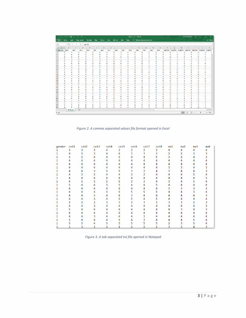
c. Connect to WEB GESCA
i. Open your web browser, e.g., Google Chrome, Microsoft Edge, Firefox, etc.
Figure 4. Web browser
ii. Enter ‘http://sem-gesca.com/webgesca/’ or ‘http://sem-gesca.org/webgesca/’ in
the address area.
Figure 5. Address for WEB GESCA

5 | P a g e
iii. Now you can see the front page of WEB GESCA.
Figure 6. Front page of WEB GESCA
d. Data
The page ‘Data’ is the first page when you visit WEB GESCA. The first step for
running WEB GESCA is upload your data, which are already prepared as described in
Section 2.b. You can also download sample data by clicking the button.
i. Upload data file
- Click the ‘Browse’ button and select a data file of your choosing.
Figure 7. Upload data file (step 1)
- Select your data file and click the open button in the window. If the file is
successfully uploaded, you will see the first six cases of the data. The Model
menu will also become available in the left-hand sidebar.

6 | P a g e
Figure 8. Upload data file (step 2)
ii. Input specifications
Once the data is uploaded, you can specify your input data on the right-hand side
of the Data page. The default set up is ‘data has header’ and ‘it is separated by
comma.’ If your data is not formatted as required, the data will not appear
appropriately in the ‘First 6 cases of the data’ area. Note that if you uncheck the
checkbox for header because your data doesn’t contain the names of indicators, the
program will assign arbitrary names to them.
Figure 9. Input specification.

7 | P a g e
iii. Missing Data
WEB GESCA currently provides users with three options for dealing with missing
observations: (1) listwise deletion, (2) mean substitution, and (3) least-squares
imputation (refer to Hwang & Takane, 2014, Chapter 3). Users can select one of
the options in the box of “Missing Data” on the right side of the page. Once users
select an option for missing data, another box “Missing value identifier” will
appear, where users input a numeric value that indicates missing observations in
their data. The default value indicating missing observations is -9999. However,
users can put any value of their choosing.
Figure 10. Handling missing data
iv. Analysis Type
If you want to conduct a multi-group analysis, choose ‘Multi-group analysis’.
Once you check the check box, all variables’ names of your data will appear.
Please select a variable that you want to use as a grouping variable from those
listed.
Figure 11. Options for multi-group analysis

8 | P a g e
e. Model
After uploading and specifying data, you need to specify your model. Click Model in
the left main menu. There are two ways to build your model: using gesca R syntax or
Table. If you are familiar with gesca R syntax and want to use the syntax, select the
tab ‘Build a model by syntax’ on the top. Otherwise, select the tab ‘Build a model by
table.’
Figure 12. Two methods for modeling
i. Build a model by syntax
This is the simplest way to run WEB GESCA. Simply enter your measurement
model and structural model into the textbox of ‘Input your model.’ After you input
the syntax, click the button. Then, WEB GESCA will run to analyze
your model. Please refer to gesca R package manual for the use of gesca R syntax
(https://cran.r-project.org/web/packages/gesca/gesca.pdf).
Figure 13. Build a model by syntax

9 | P a g e
ii. Build a model by table
1) Choose the number of latent variables
Drag the slider to choose the number of latent variables in your model. If your
model has second-order latent variables, choose the number of them as well.
After choosing the number of latent variables, click ‘Confirm the number of
latent variables’.
Figure 14. Select number of latent variables
2) Input names of latent variables
If you confirmed the number of latent variables, the box for inputting the name
of each latent variable will appear. Input the names of your latent variables. If
you don’t label your latent variables, they will be named like LV_1, LV_2, …
LV_n by default.
Figure 15. Naming for latent variables
If all the names of latent variables are entered correctly, then please click
‘confirm the name(s)’.

10 | P a g e
3) Specifying structural model
Once you confirmed latent variables’ names, a table for specifying your
structural model will appear in the middle of the main contents area. You can
specify a structural model by checking checkboxes. The figure below shows
that LV_1 affects LV_2.
Figure 7. Specifying structural model
If you want to fix a path coefficient to a constant, enter the constant value
ranging from 0.0 to 1.0 to the blank textbox.
Figure 8. Fixing path coefficient
If you selected ‘multi-group analysis’ (2.e.iii), you can constrain all path
coefficients to be equal across groups simultaneously by checking ‘Constraining
path coefficients across groups.’ This checkbox only appears when you selected
multi-group analysis.
Figure 98. Constraining all path coefficients across groups

11 | P a g e
After you completed structural model specification, click ‘confirm the model.’
4) Assigning indicators
You can assign indicators to latent variables by using the checkboxes.
Figure 10. Assigning indicators
Figure 19 shows that the latent variable LV_1 is assigned the indicators cei1,
cei2, and cei3, LV_2 is assigned cei4, cei5, and cei6, and LV_3 is assigned cei7,
cei8 and ma1.
If you want to fix a loading to a constant in advance, put the constant value
ranging from 0.0 to 1.0 in the blank textbox.
Figure 20. Fixing value of loading for an indicator

12 | P a g e
If you selected multi-group analysis (2.e.iii), you have two more options for
constrained analyses. First, you can constrain the loadings of selected indicators to be
identical by inserting a label (e.g., an alphabet letter or number) across groups. In the
below example, three indicators were chosen, and labeled by different alphabet
letters (“a”, “b”, and “c”). This indicates that each loading of the three indicators is
to be held equal across groups. Note that any loadings with the same label will be
constrained to be equal to each other.
Figure 21. Constraining specific loadings across group
Also, if you choose ‘Constraining (fix) loadings across groups,’ all loadings will
be constrained to be equal across groups.
Figure 22. Constraining all loadings across group

13 | P a g e
If formative indicators are assumed for a latent variable, you check the
‘Formative relationship’ box per latent variable located at the top of the table. If
they are reflective indicators, just leave the checkboxes unchecked.
Figure 23. Specifying formative relationship between the indicators and the latent variable
The above figure shows that cei1, cei2, and cei3 are formative indicators for
LV_1, whereas the remaining indicators for LV_2 and LV_3 are reflective.
5) Second-order latent variable modeling
If you have a second-order latent variable in your model (2.f.ii), you need to
specify the relationship between second-order and first-order latent variables.
Another table will appear below the table for assigning indicators if your model
has a second-order latent variable. The below figure shows that a second-order
latent variable, LV2_1, is related to its lower-order latent variables LV_2 and
LV_3, which serve as formative indicators for LV2_1.
Figure 24. Specifying relation between second-order latent variable and lower-order latent variables

14 | P a g e
iii. Analyze Model
Once you have finished all your model specification (either using syntax or table),
please click . WEB GESCA will run your model. When the analysis is
complete without any errors, you will see Summary, Parameter Estimates, and
Plots appear on the main menu.
f. Summary
On the summary page, you can see Estimation Summary and Model Fit.
Figure 25. Summary of the analysis
g. Parameter estimates
This page shows each parameter estimate.
Figure 26. Parameter estimates for loading

15 | P a g e
h. Plots
This page displays the same parameter estimates graphically.
Figure 27. Plots for parameter estimation (weight)
i. Qualitative Measures
This page shows a variety of reliability and validity measures.
Figure 28. A variety of reliability and validity measures

16 | P a g e
j. Effects
This page shows following total and indirect effects of variables
- Total effects of latent variables (Std. Error)
- Indirect effects of latent variables (Std. Error)
- Total effects of latent variables on indicators (Std. Error)
- Indirect effects of latent variables on indicators (Std. Error)
Figure 29. Total effects of latent variables (Std. Error) and Indirect effects of latent variables (Std. Error)
Figure 30. Total effects of latent variables on indicators (Std. Error)
17 | P a g e
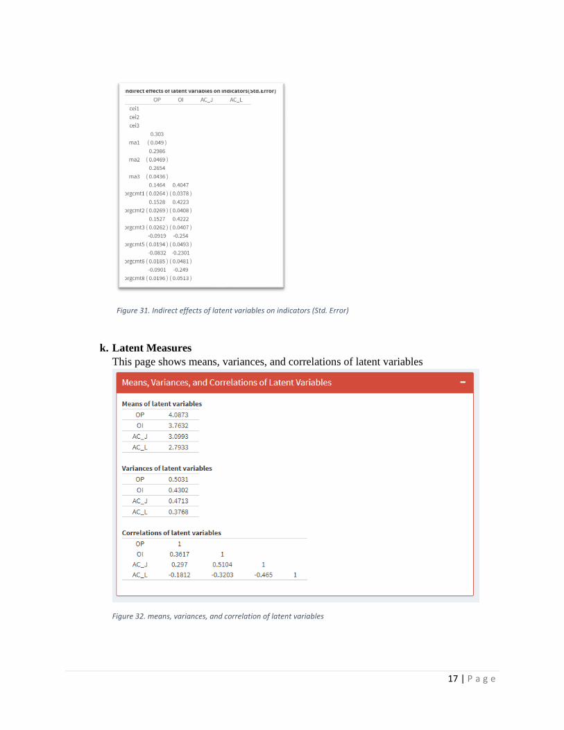
Figure 31. Indirect effects of latent variables on indicators (Std. Error)
k. Latent Measures
This page shows means, variances, and correlations of latent variables
Figure 32. means, variances, and correlation of latent variables

18 | P a g e
2. How to interpret the results
Table 1. Model fit of the result
Model Fit
FIT .535
AFIT .532
GFI .993
SRMR .078
FIT_M .606
FIT_S .168
Table 1. provides six measures of model fit.
• FIT indicates the total variance of all variables explained by a model specification.
The values of FIT range from 0 to 1. The larger this value, the more variance in the
variables is accounted for by the specified model.
• AFIT (Adjusted FIT) is similar to FIT, but takes model complexity into account. The
AFIT may be used for model comparison. The model with the largest AFIT value
may be chosen among competing models.
• (Unweighted least-squares) GFI and SRMR (standardized root mean square
residual). Both are proportional to the difference between the sample covariances and
the covariances reproduced by the parameter estimates of generalized structured
component analysis. The GFI values close to 1 and the SRMR values close to 0 may
be taken as indicative of good fit.
• FIT_M signifies how much the variance of indicators is explained by a measurement
model
• FIT_S indicates how much the variance of latent variable is accounted for by a
structural model. Both FIT_M and FIS_S can be interpreted in a manner similar to
the FIT.

19 | P a g e
Table 2. Parameter Estimates of Loadings
Loadings
Estimate SE 95% CI_LB 95% CI_UB
cei1 .781 .025 .716 .831
cei2 .825 .021 .786 .854
cei3 .770 .029 .703 .820
cei4 .804 .030 .727 .868
cei5 .801 .028 .741 .846
cei6 .843 .028 .796 .883
cei7 .776 .024 .728 .824
cei8 .801 .033 .705 .856
ma1 .787 .026 .731 .825
ma2 .758 .025 .700 .805
ma3 .637 .039 .547 .704
ma4 .823 .028 .761 .803
ma5 .811 .024 .757 .849
ma6 .743 .040 .675 .793
orgcmt1 .748 .036 .675 .795
orgcmt2 .790 .024 .747 .834
orgcmt3 .820 .020 .773 .857
orgcmt7 .707 .033 .620 .778
orgcmt5 .796 .029 .721 .842
orgcmt6 .709 .050 .597 .796
orgcmt8 .782 .030 .726 .843
Table 2 displays the estimates of loadings and their bootstrap standard errors (SEs), and
95% confidence intervals. (Note: when indicators are formative, their loading estimates
will not be reported)

20 | P a g e
Table 3. Parameter Estimates of weights
Weights
Estimate SE 95% CI_LB 95% CI_UB
cei1 .150 .010 .132 .170
cei2 .160 .010 .141 .179
cei3 .157 .010 .140 .177
cei4 .147 .009 .126 .163
cei5 .162 .011 .143 .184
cei6 .168 .009 .153 .191
cei7 .150 .009 .130 .167
cei8 .154 .009 .140 .168
ma1 .219 .021 .182 .263
ma2 .211 .020 .175 .252
ma3 .194 .017 .163 .233
ma4 .261 .019 .228 .293
ma5 .237 .019 .199 .267
ma6 .184 .021 .150 .238
orgcmt1 .302 .018 .263 .348
orgcmt2 .330 .016 .296 .371
orgcmt3 .364 .019 .337 .400
orgcmt7 .303 .018 .257 .344
orgcmt5 .453 .025 .403 .500
orgcmt6 .387 .026 .328 .441
orgcmt8 .467 .031 .420 .529
Table 3 displays the estimates of weights and their bootstrap standard errors (SEs), and
95% confidence intervals
Table 4. Parameter estimates of path coefficients
Path Coefficients
Estimate SE 95% CI_LB 95% CI_UB
LV_1 ~ LV_2 .362 .067 .260 .465
LV_2 ~ LV_3 .614 .042 .549 .678
LV_2 ~ LV_4 -.404 .049 -.515 -.288
Table 4. shows the estimates of path coefficients and their bootstrap standard errors (SE)
and 95% confidence intervals.

21 | P a g e
Table 5. R squares of latent variables
R squares of Latent Variables
LV_1 0
LV_2 .131
LV_3 .377
LV_4 .163
Table 5 provides the R square values of each “endogenous” latent variable, indicating
how much variance of an endogenous latent variable is explained by its exogenous latent
variables. In the present example, the first latent variable (LV_1) is exogenous, so that its
R square is zero.
Table 6. Reliability and validity of measures
Cronbach’s
alpha
Dillon-
Goldstein’s rho AVE
Number of eigenvalues
greater than one per block
of indicators
LV_1 .8242 .8956 .7414 1
LV_2 .7173 .8419 .6404 1
LV_3 .7492 .8567 .6659 1
LV_4 .6418 .8071 .5828 1
In Table 6 Cronbach’s alpha and Dillon-Goldstein’s rho (or the composite reliability) can
be used for checking internal consistency of indicators for each latent variable. The
average variance extracted (AVE) can be used to examine the convergent validity of a
latent variable. The number of eigenvalues greater than one per block of indicators can be
used to check uni-dimensionality of the indicators.
Table 7. Correlations of Latent Variables (SE)
Correlations of Latent Variables
LV_1 LV_2 LV_3 LV_4
LV_1 1
LV_2 .362 1
LV_3 .388 .614 1
LV_4 -.209 -.404 -.461 1
Table 7 shows the correlations among latent variables.


![ga [ca] - textred.spanport.lss.wisc.edu · geronte geróntico gerontocracia gerontófago gerontofobia gerontológico gerontólogo gerundiado gerundio gesca gesnereácea [gesneriácea]](https://img.pdfslide.net/doc/110x75/5bdc916109d3f2a5128b7de7/ga-ca-geronte-gerontico-gerontocracia-gerontofago-gerontofobia-gerontologico.jpg)