Web Extension: Continuous Distributions and Estimating Beta with a

2C H A P T E R

2E-1

Web Extension: Continuous Distributions and Estimating Beta with a Calculator

This extension explains continuous probability distributions and provides a brief tutorial onusing financial calculators to calculate beta coefficients.

Continuous Probability DistributionsIn Chapter 2, we illustrated risk/return concepts using discrete distributions, andwe assumed that only three states of the economy could exist. In reality, however,the state of the economy can range from a deep recession to a fantastic boom, andthere is an infinite number of possibilities in between. It is inconvenient to workwith a large number of outcomes using discrete distributions, but it is relativelyeasy to deal with such situations with continuous distributions since many suchdistributions can be completely specified by only two or three summary statisticssuch as the mean (or expected value), standard deviation, and a measure of skew-ness. In the past, financial managers did not have the tools necessary to use con-tinuous distributions in practical risk analyses. Now, however, firms have access tocomputers and powerful software packages, including spreadsheet add-ins, whichcan process continuous distributions. Thus, if financial risk analysis is computer-ized, as is increasingly the case, it is often preferable to use continuous distribu-tions to express the distribution of outcomes.1

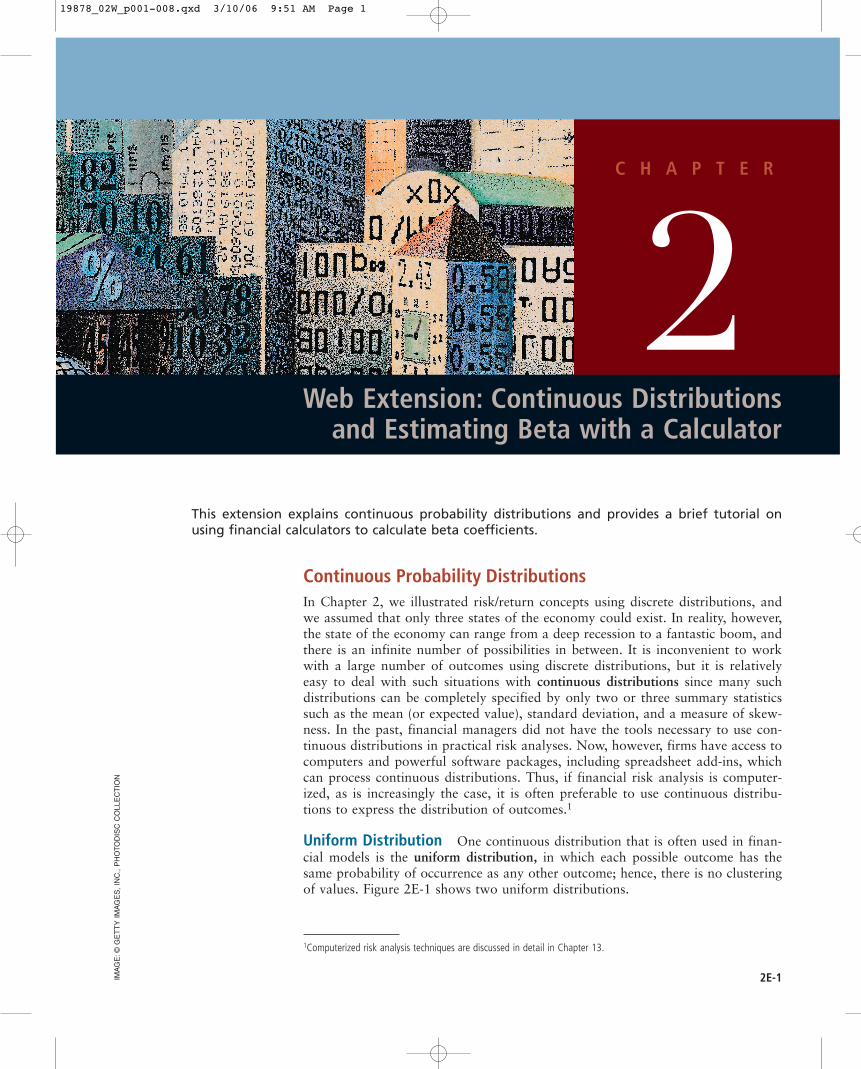
Uniform Distribution One continuous distribution that is often used in finan-cial models is the uniform distribution, in which each possible outcome has thesame probability of occurrence as any other outcome; hence, there is no clusteringof values. Figure 2E-1 shows two uniform distributions.

IMA

GE

:©G

ET

TY

IM

AG

ES

, IN

C.,

PH

OTO

DIS

C C

OLL

EC

TIO

N

1Computerized risk analysis techniques are discussed in detail in Chapter 13.

19878_02W_p001-008.qxd 3/10/06 9:51 AM Page 1

2E-2 • Chapter 2 Web Extension: Continuous Distributions and Estimating Beta with a Calculator

Distribution A of Figure 2E-1 has a range of �5 to �15 percent. Therefore,the absolute size of the range is 20 units. Since the entire area under the densityfunction must equal 1.00, the height of the distribution, h, must be 0.05: 20h � 1.0,so h � 1/20 � 0.05. We can use this information to find the probability of differ-ent outcomes. For example, suppose we want to find the probability that the rateof return will be less than zero. The probability is the area under the density func-tion from �5 to 0 percent; that is, the shaded area:

Area � (Right point � Left point)(Height of distribution)� [0 � (�5)][0.05] � 0.25 � 25%

Similarly, the probability of a rate of return between 5 and 15 is 50 percent:

Probability � Area � (15 � 5)(0.05) � 0.50 � 50%.

The expected rate of return is the midpoint of the range, or 5 percent, forboth distributions in Figure 2E-1. Since there is a smaller probability of the actualreturn falling very far below the expected return in Distribution B, Distribution Bdepicts a less risky situation in the stand-alone risk sense.

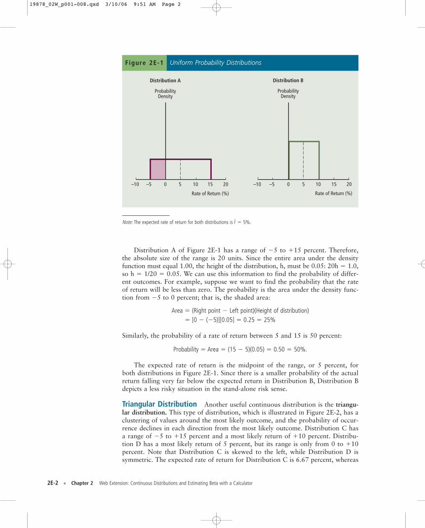
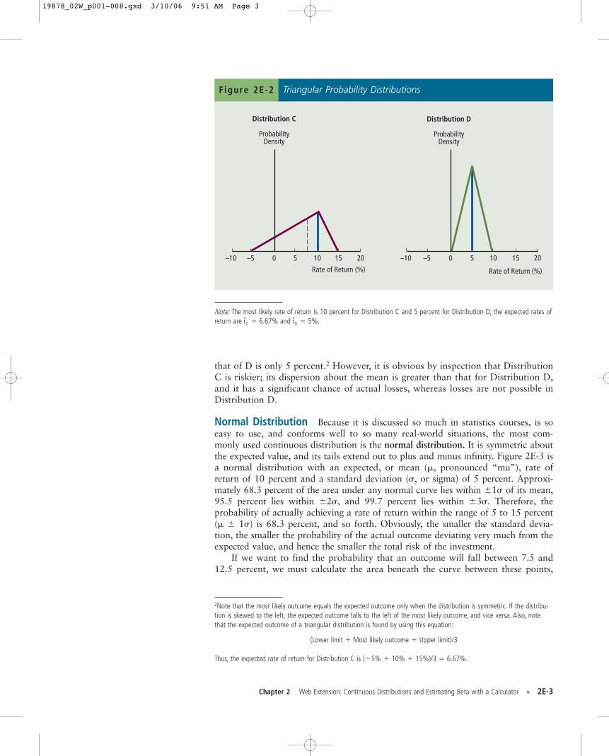
Triangular Distribution Another useful continuous distribution is the triangu-lar distribution. This type of distribution, which is illustrated in Figure 2E-2, has aclustering of values around the most likely outcome, and the probability of occur-rence declines in each direction from the most likely outcome. Distribution C hasa range of �5 to �15 percent and a most likely return of �10 percent. Distribu-tion D has a most likely return of 5 percent, but its range is only from 0 to �10percent. Note that Distribution C is skewed to the left, while Distribution D issymmetric. The expected rate of return for Distribution C is 6.67 percent, whereas

Distribution A

ProbabilityDensity

–10 –5 0 5 10 15 20

Distribution B

ProbabilityDensity

–10 –5 0 5 10 15 20

Rate of Return (%)Rate of Return (%)

Uniform Probability DistributionsFigure 2E-1

Note: The expected rate of return for both distributions is r � 5%.

19878_02W_p001-008.qxd 3/10/06 9:51 AM Page 2

Chapter 2 Web Extension: Continuous Distributions and Estimating Beta with a Calculator • 2E-3

that of D is only 5 percent.2 However, it is obvious by inspection that DistributionC is riskier; its dispersion about the mean is greater than that for Distribution D,and it has a significant chance of actual losses, whereas losses are not possible inDistribution D.

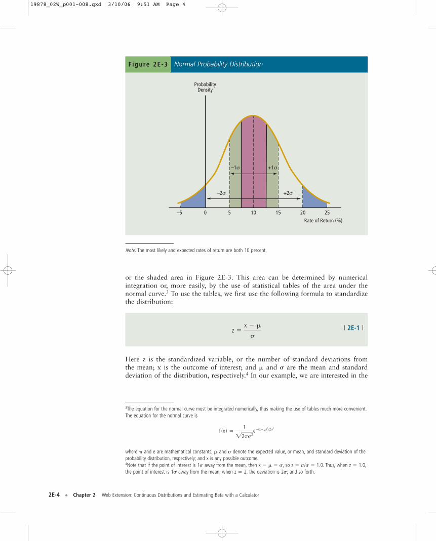
Normal Distribution Because it is discussed so much in statistics courses, is soeasy to use, and conforms well to so many real-world situations, the most com-monly used continuous distribution is the normal distribution. It is symmetric aboutthe expected value, and its tails extend out to plus and minus infinity. Figure 2E-3 isa normal distribution with an expected, or mean (�, pronounced “mu”), rate ofreturn of 10 percent and a standard deviation (�, or sigma) of 5 percent. Approxi-mately 68.3 percent of the area under any normal curve lies within �1� of its mean,95.5 percent lies within �2�, and 99.7 percent lies within �3�. Therefore, theprobability of actually achieving a rate of return within the range of 5 to 15 percent(� � 1�) is 68.3 percent, and so forth. Obviously, the smaller the standard devia-tion, the smaller the probability of the actual outcome deviating very much from theexpected value, and hence the smaller the total risk of the investment.

If we want to find the probability that an outcome will fall between 7.5 and12.5 percent, we must calculate the area beneath the curve between these points,

Distribution C

ProbabilityDensity

–10 –5 0 5 10 15 20

Distribution D

ProbabilityDensity

–10 –5 0 5 10 15 20

Rate of Return (%)Rate of Return (%)

Triangular Probability DistributionsFigure 2E-2

Note: The most likely rate of return is 10 percent for Distribution C and 5 percent for Distribution D; the expected rates ofreturn are rC � 6.67% and rD � 5%.

2Note that the most likely outcome equals the expected outcome only when the distribution is symmetric. If the distribu-tion is skewed to the left, the expected outcome falls to the left of the most likely outcome, and vice versa. Also, notethat the expected outcome of a triangular distribution is found by using this equation:

(Lower limit � Most likely outcome � Upper limit)/3

Thus, the expected rate of return for Distribution C is (�5% � 10% � 15%)/3 � 6.67%.

19878_02W_p001-008.qxd 3/10/06 9:51 AM Page 3


or the shaded area in Figure 2E-3. This area can be determined by numericalintegration or, more easily, by the use of statistical tables of the area under thenormal curve.3 To use the tables, we first use the following formula to standardizethe distribution:

| 2E-1 |

Here z is the standardized variable, or the number of standard deviations fromthe mean; x is the outcome of interest; and � and � are the mean and standarddeviation of the distribution, respectively.4 In our example, we are interested in the

z �x � �

�

–5 0 5 10 15 20 25

ProbabilityDensity

–1σ

Rate of Return (%)

+1σ

–2σ +2σ

Normal Probability DistributionFigure 2E-3

Note: The most likely and expected rates of return are both 10 percent.

3The equation for the normal curve must be integrated numerically, thus making the use of tables much more convenient.The equation for the normal curve is

where � and e are mathematical constants; � and � denote the expected value, or mean, and standard deviation of theprobability distribution, respectively; and x is any possible outcome.4Note that if the point of interest is 1� away from the mean, then x � � � �, so z � �/� � 1.0. Thus, when z � 1.0,the point of interest is 1� away from the mean; when z � 2, the deviation is 2�; and so forth.

f (x ) �1

22��2e�(x��)2>2�2

19878_02W_p001-008.qxd 3/10/06 9:51 AM Page 4


probability that an outcome will fall between 7.5 and 12.5 percent. Since themean of the distribution is 10, and it is between the two points of interest, wemust evaluate and then combine two probabilities, one to the left and one to theright of the mean. We first normalize these points by using Equation 2E-1:

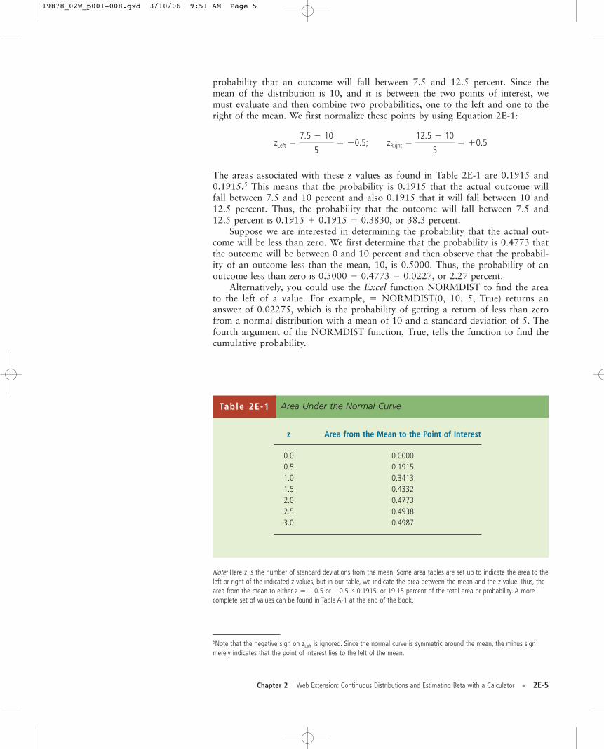
The areas associated with these z values as found in Table 2E-1 are 0.1915 and0.1915.5 This means that the probability is 0.1915 that the actual outcome willfall between 7.5 and 10 percent and also 0.1915 that it will fall between 10 and12.5 percent. Thus, the probability that the outcome will fall between 7.5 and12.5 percent is 0.1915 � 0.1915 � 0.3830, or 38.3 percent.

Suppose we are interested in determining the probability that the actual out-come will be less than zero. We first determine that the probability is 0.4773 thatthe outcome will be between 0 and 10 percent and then observe that the probabil-ity of an outcome less than the mean, 10, is 0.5000. Thus, the probability of anoutcome less than zero is 0.5000 � 0.4773 � 0.0227, or 2.27 percent.

Alternatively, you could use the Excel function NORMDIST to find the areato the left of a value. For example, � NORMDIST(0, 10, 5, True) returns ananswer of 0.02275, which is the probability of getting a return of less than zerofrom a normal distribution with a mean of 10 and a standard deviation of 5. Thefourth argument of the NORMDIST function, True, tells the function to find thecumulative probability.

zRight �12.5 � 10

5� �0.5zLeft �

7.5 � 10

5� �0.5;

5Note that the negative sign on zLeft is ignored. Since the normal curve is symmetric around the mean, the minus signmerely indicates that the point of interest lies to the left of the mean.

Area Under the Normal CurveTable 2E-1

z Area from the Mean to the Point of Interest

0.0 0.00000.5 0.19151.0 0.34131.5 0.43322.0 0.47732.5 0.49383.0 0.4987

Note: Here z is the number of standard deviations from the mean. Some area tables are set up to indicate the area to theleft or right of the indicated z values, but in our table, we indicate the area between the mean and the z value. Thus, thearea from the mean to either z � �0.5 or �0.5 is 0.1915, or 19.15 percent of the total area or probability. A morecomplete set of values can be found in Table A-1 at the end of the book.

19878_02W_p001-008.qxd 3/10/06 9:51 AM Page 5


Using Continuous Distributions Continuous distributions are generally usedin financial analysis in the following manner:

1. Someone with a good knowledge of a particular situation is asked to specifythe most applicable type of distribution and its parameters. For example, acompany’s marketing manager might be asked to supply this information forsales of a given product, or an engineer might be asked to estimate the con-struction costs of a capital project.

2. A financial analyst could then use these input data to help evaluate the riskinessof a given decision. For example, the analyst might conclude that the proba-bility is 50 percent that the actual rate of return on a project will be between5 and 10 percent, that the probability of a loss (negative rate of return) on theproject is 15 percent, or that the probability of a return greater than 10 per-cent is 25 percent. Generally, such an analysis would be done by using a com-puter program.

In theory, we should use the specific distribution that best represents the truesituation. Sometimes the true distribution is known, but with most financial data,it is not known. For example, we might think that interest rates could range from8 to 15 percent next year, with a most likely value of 10 percent. This suggests atriangular distribution. Or we might think that interest rates next year can best berepresented by a normal distribution, with a mean of 10 percent and a standarddeviation of 2.5 percent. The point is, there is simply no type of distribution thatis always “best”; you need to be familiar with different types of distributions andtheir properties, and then you must select the best distribution for the problemat hand.

Calculating Beta Coefficients with a Financial CalculatorFollowing are brief descriptions of using a financial calculator to calculate betacoefficients. See your owner’s manual or our Technology Supplement, availablefrom your professor, for more details.

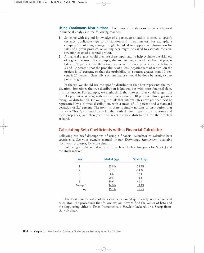
Following are the actual returns for each of the last five years for Stock J andthe stock market:

Year Market ( r–M) Stock J ( r–J)

1 23.8% 38.6%2 (7.2) (24.7)3 6.6 12.34 20.5 8.25 30.6 40.1

Average r 14.9% 14.9%� r 15.1% 26.5%

The least squares value of beta can be obtained quite easily with a financialcalculator. The procedures that follow explain how to find the values of beta andthe slope using either a Texas Instruments, a Hewlett-Packard, or a Sharp finan-cial calculator.

19878_02W_p001-008.qxd 3/10/06 9:51 AM Page 6


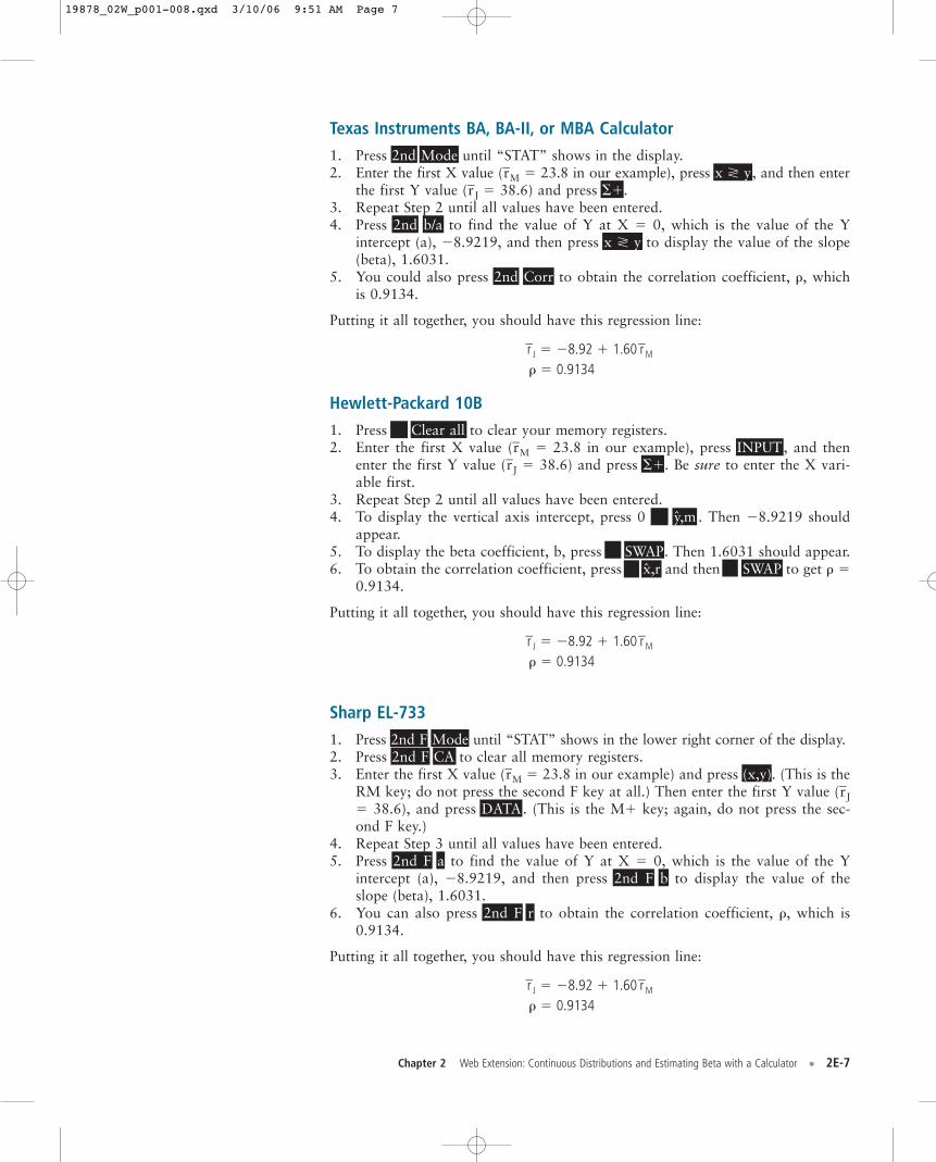
Texas Instruments BA, BA-II, or MBA Calculator

1. Press 2nd Mode until “STAT” shows in the display.2. Enter the first X value (rM � 23.8 in our example), press x y, and then enter

the first Y value (rJ � 38.6) and press ��.3. Repeat Step 2 until all values have been entered.4. Press 2nd b/a to find the value of Y at X � 0, which is the value of the Y

intercept (a), �8.9219, and then press x y to display the value of the slope(beta), 1.6031.

5. You could also press 2nd Corr to obtain the correlation coefficient, �, whichis 0.9134.

Putting it all together, you should have this regression line:

rJ � �8.92 � 1.60 rM

� � 0.9134

Hewlett-Packard 10B

1. Press Clear all to clear your memory registers.2. Enter the first X value (rM � 23.8 in our example), press INPUT, and then

enter the first Y value (rJ � 38.6) and press ��. Be sure to enter the X vari-able first.

3. Repeat Step 2 until all values have been entered.4. To display the vertical axis intercept, press 0 y,m . Then �8.9219 should

appear.5. To display the beta coefficient, b, press SWAP. Then 1.6031 should appear.6. To obtain the correlation coefficient, press x,r and then SWAP to get � �

0.9134.


rJ � �8.92 � 1.60 rM

� � 0.9134

Sharp EL-733

1. Press 2nd F Mode until “STAT” shows in the lower right corner of the display.2. Press 2nd F CA to clear all memory registers.3. Enter the first X value (rM � 23.8 in our example) and press (x,y). (This is the

RM key; do not press the second F key at all.) Then enter the first Y value (rJ� 38.6), and press DATA. (This is the M� key; again, do not press the sec-ond F key.)

4. Repeat Step 3 until all values have been entered.5. Press 2nd F a to find the value of Y at X � 0, which is the value of the Y

intercept (a), �8.9219, and then press 2nd F b to display the value of theslope (beta), 1.6031.

6. You can also press 2nd F r to obtain the correlation coefficient, �, which is0.9134.


rJ � �8.92 � 1.60 rM

� � 0.9134

19878_02W_p001-008.qxd 3/10/06 9:51 AM Page 7


Beta coefficients can also be calculated with spreadsheet programs such asExcel. Simply input the returns data and then use the spreadsheet’s regression rou-tine or SLOPE function to calculate beta. The model on the file named IFM9 Ch02Tool Kit.xls calculates beta for our illustrative Stock J, and it produces exactly thesame results as with the calculator. However, the spreadsheet is more flexible.First, the file can be retained, and when new data become available, they can beadded and a new beta can be calculated quite rapidly. Second, the regression out-put can include graphs and statistical information designed to give us an idea ofhow stable the beta coefficient is. In other words, while our beta was calculated tobe 1.60, the “true beta” might actually be higher or lower, and the regression out-put can give us an idea of how large the error might be. Third, the spreadsheet canbe used to calculate returns data from historical stock price and dividend informa-tion, and then the returns can be fed into the regression routine to calculate thebeta coefficient. This is important, because stock market data are generally pro-vided in the form of stock prices and dividends, making it necessary to calculatereturns. This can be a big job if a number of different companies and a number oftime periods are involved.

19878_02W_p001-008.qxd 3/10/06 9:51 AM Page 8

Documents

Web Extension: Continuous Distributions and Estimating Beta with a