Chapter 17

Cube Calculus MachineMarek Perkowski and Qihong Chen

The software-based approach is the simplest and cheapest way to realize cube calculus operations. Since the algorithm of a sequential cube calculus operation involves several levels of nested loops, it leads to poor performance on general purpose computers. In some applications, such as logic minimization systems, or logic-based machine learning systems, there are so many cube calculus operations, that the software-based approach makes those applications unacceptable for practical sized problems due to poor performance. For speeding up the cube calculus operations, the cube calculus machine was invented. Several version of this machine were built at PSU [ref,ref].

17.1. Formalism for main algorithm for cube calculus operation

The architecture of the Cube Calculus Machine (CCM) results from an attempt to optimize the execution of the most complex cube operation, sequential cube calculus operations, like crosslink and sharp. Almost all cube calculus operations have two operand cubes described in Formulas 17.3 and 17.4.

We re-write these two operand cubes in positional notation as:

17.1.

where , which is the true set of literal in

positional notation. For each bit from . The bit represents the m-th

possible value of the i-th variable. Similarly, and

for each bit bi,m from . Example 17.18 shows how to use this notation.

The sequential cube operations are generally described by Equation 17.12. We can re-write the equation in positional notation as:

17.2

Where resultant array of cubes is:

17.3.

where bef, act and aft are bitwise functions used to calculate set operations before, active and after, respectively. As discussed in section 17.4, an important property of output functions bef, act and aft is that they are bitwise functions.

As discussed in section 17.4.3, the relation function is broken down into two parts: partial relation and relation type. There are only two possible relation types: AND and OR. The relation can be described by:

17.4.

Where rel is the partial relation and it is bitwise function.

All simple combinational cube operations can be defined as a single set operation (see section 2.3.1), so there is no need to define before, active and after functions. For consistency of description, however, we will assume that all variables in the case of the combinational cube calculus operations are of the before type. This way, the same computational mechanism can be used to calculate the combinational cube calculus operations. Therefore, combinational operations can be described by the following equation:

17.5.

All complex combinational cube operations are defined by two set operations and one set relation (see section 17.3.2). For consistency of description, the complex combinational cube operations can be described by:

17.6.

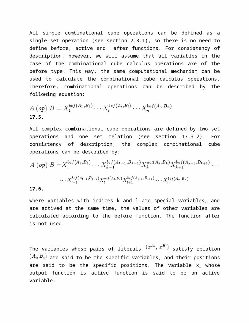
where variables with indices k and l are special variables, and are actived at the same time, the values of other variables are calculated according to the before function. The function after is not used.

The variables whose pairs of literals satisfy relation are said to be the specific variables, and their positions are said to be the specific positions. The variable x i whose output function is active function is said to be an active variable.

In the case of sequential cube operations, there is only one active variable at a time. In the case of complex combinational cube operations, it is possible to have multiple active variables at the same time.

From the above discussion, we can see that these cube operations can be described by functions relation, before, active and after, and have similar formulas.

17.2. The general programmable patterns

The bitwise function (of length k) is the k-time repetition of the same two-input, one-output

Boolean function on argument vectors. For instance, the bitwise function is defined as follows:

where are the vectors

, respectively. In cube operations, there are four bitwise functions: before, active, after and rel (partial relation).

We can use a truth table to specify the output values for a Boolean function in terms of the values of input variables. For a bitwise function, there are 2 * 2=4 combinations of values of the variables. Therefore, the bitwise function can be completely specified by its four output values. This is shown in Figure 17.1(a).

An arbitrary Boolean function of two binary variables a and b can be realized by a 4-to-1 multiplexer as shown in Figure 17.1(b). The variables a and b are the control inputs of the multiplexer, the output values of the function are the data inputs of the multiplexer. The values of a and b will select the valid output values from the data inputs.

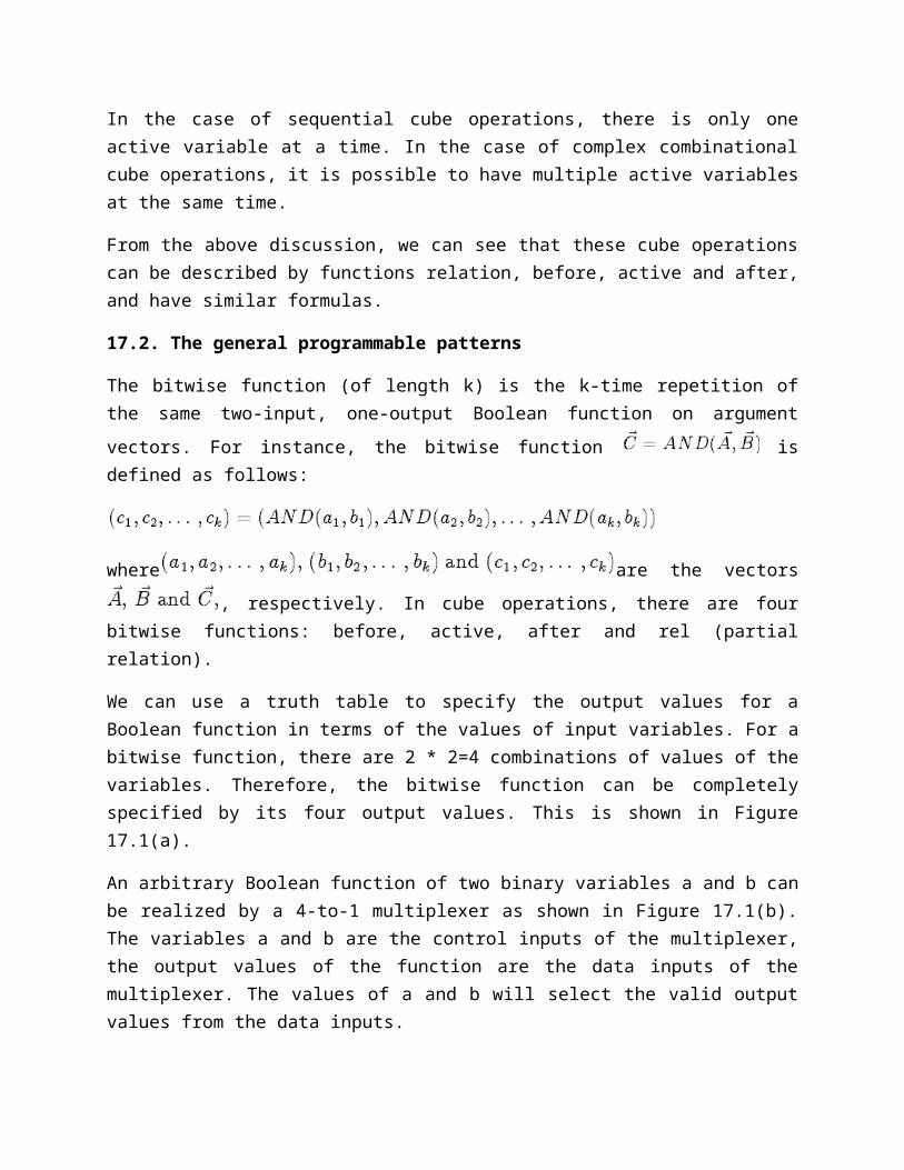
Figure 17.1. Realizing an arbitrary function of two binary variables

This general structure can be programmed to realize an arbitrary bitwise function. For example, the output values of function f(a,b)=a+b are 0111. Set I0I1I2I3=0111, the output of multiplexer is the function of f(a,b) = a+b.

We derived all output values of the bitwise functions of the cube operations listed in Table 17.4, the results are listed in Table 17.1. This calculation is very simple. For example, suppose the

function is , then

Therefore, the output values of function are 0010.

Each row of Table 17.1 describes one cube operation. The operation name, notation, the output value of rel (partial relation) function, and_or (relation type), the output values of before, active and after functions are listed from left to right. The value of and_or equals to 1 means that the relation type is of AND type; otherwise, the relation type is of OR type.

17.3. The data path of CCM

Since the data path of CCM results from an attempt to optimize the execution of cube calculus operations, especially the sequential cube calculus operations, the CCM has been designed to directly implement Formulas 17.2 and 17.3.

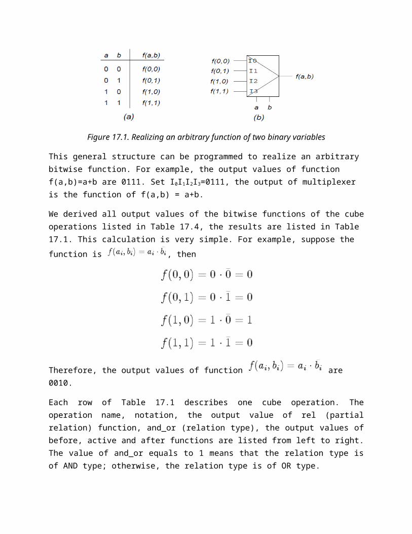
Table 17.1. The output Values of Bitwise Functions Used in Cube Operations

From Formula 17.3, it can be seen that one relation function and one of three output functions

(bef, act and aft) are applied on every pair of literals in the same manner. This means that we can use one combinational logic block to process every pair of literals in series, or use n identical logic blocks to process all pairs of literals in parallel (one pair of literals per logic block). Obviously, you recognize that this second solution is the familiar to you iterative network. It has a better performance than the former because of its parallelism. The CCM is realized using an iterative network. Before we describe the architecture of the CCM, let us take a look at the general concept of the iterative networks.

17.3.1. Iterative Network

An iterative network consists of a number of identical cells interconnected in a regular manner. Some operations, like binary addition, are naturally realized with an iterative network because the same operation is performed on each pair of input bits.

The simplest form of iterative network consists of a linear array of combinational cells with signals between cells traveling in only one direction.

As shown in Figure 17.2 each cell is a combinational network with one or more primary input(s) (x[i]) and possibly one or more primary output[s] (z[i]). In addition, each cell has one or more secondary input(s) (a[i]) and one or more secondary output(s) (a[i+1]). The a[i] leads carry information about the “state” of the previous cell. The primary inputs to the cells (x[1], x[2], …… x[n]) are applied in parallel, that is, they are applied at the same time. The a[i] signals then propagate down the line of cells. Since the network is combinational, the time required for the network to reach a stable state condition is determined only by the delay times of the gates in the cells. As soon as stable state is reached, the output may be read.

Therefore, the iterative network can function as a parallel input, parallel-output device, in contrast with the sequential network in which the input and output are provided in a serial manner.

Example 17.1. The Parity Checker determines whether the number or 1’s in a n-bit word is even or odd. The Figure3.3 shows the complete iterative network for n = 4. The output of it will be 1 if an odd number of x inputs are 1. The logic of a cell can be described by

a[i] = a[i] x[i]

Assuming the delay of a cell (an EXOR gate in this example) is tcell. The a[1] input to the first cell must be since no ones are received to the left of the first cell and is an even number. The delay of the output of the last cell a[5] is 4tcell in this example.

Figure 17.3. Parity Checker

Example 17.2. The Ripple-carry binary adder is used to perform addition on two binary numbers. A 4 bits adder can be constructed by cascading 4 full-adder circuit in series as shown in Figure 17.4. The logic of a full adder can be described by

c[i+1] = g[i] + p[i]c[i]s[i] = p[i] c[i]

where c[i], c[i+1] and s are carry input, carry output and sum output of cell i, respectively. g (generate) and p (propagate) are two intermediate signals and can be described by

g[i] = a[i]. b[i]p[i] = a[i] b[i].

Figure 17.4. Ripple-Carry Binary Adder

Assuming the delay from inputs (a[i] and b[i]) to intermediate signals (g and p) is t1, and from intermediate signals and carry input (c[i]) to the outputs (c[i+1) and s[i]) is t2, and the input c[0] is (constant). It can be seen that the carry signal is propagated from left to right along the carry chain, and the carry chain is the worst-case delay path of the adder. Thus, the delay of this adder is t1 + 4t2.

For the design cases where an iterative network can be used, it offers several advantages over an ordinary combinational network:

It is easier to design It is easily expanded to accommodate more inputs simply by adding more cells.

The principal disadvantage of the iterative network is that the signal must be propagated through a large number of cells, so the response time will be longer than in a corresponding combinational network with few levels.

17.1. The algorithm of the CCM

As mentioned above, the CCM is realized with an iterative network. The cell of this iterative network is more complex than those in the examples given in section 17.3.1. The cell of the iterative network consists of a sequential logic block and several combinational logic blocks, as shown in Figure 17.5. The inputs A[i] and B[i] are the pair of input literals. C[i] is the output literal. Relation, bef, act and aft are binary bits used to specify these function. clk and reset are the clock and reset inputs of the D flip-flops used in sequential logic block. The signal next (next[i] and next[i+1] in the figure) is the propagation signal (it will be discussed later). The signal var[i] is generated by combinational logic block A, and represents whether the variable (xi) is a special variable (var[i]=1) or not (var[i]=0).

Figure 17.5. A simplified iterative cell of CCM

For a sequential cube operation (section 17.2.3) we know that every special variable produces one resultant cube. For a given special variable (say x i), the resultant cube is generated in the following manner:

The output literal Ci is calculated by act (Ai , Bi). The output literal Ck (1 k< i) is calculated by aft(Ak, Bk). The output literal C1 (i < l n) is calculated by bef(Al, Bl). An output literal is calculated by combinational logic block B in Figure 17.5, and all output literals can be calculated in parallel with an iterative network.

A variable is to be called the active variable when it is in active state. Now we need to find a way to activate special variables in series, which means only one variable should be in an active state at a time, and all special variables become active one after another. All other variables should know their relative position with respect to the current active variable, left or right. Our solution to this problem is as follows:

• The propagation signal next activates the first special variable that it encounters. The signal next is propagated through combinational logic block C in Figure 17.5. The logic of the combinational logic block C can be described by: next[i+1] = act[i] + next[i] . var [ i] where signal act[i] is 1 when current state of the FSM is active (current state is represented by the signal state[i]).

• Every variable (cell) has a simple Finite State Machine (FSM) (the sequential logic block in the Figure 17.5) to memorize its relative position with respect to the active variable. This FSM has three states: after, active and before, which corresponds to the variable being on the left side of the active variable, the active variable itself, and the variables being on the right side of the active variable, respectively.

The state machine flowchart [22] (or SM chart for short) of the FSM is shown in Figure 17.6. The states bef, act and aft are the short name of states before, active and after, respectively. The numbers under the state names are the state assignments (the encoding vectors). This state machine is realized by using D flip-flops with asynchronous reset, thus the reset inputs of the D flip-flops can be used to reset the FSM to before state. This reset logic is not shown in the SM chart. The output of the FSM is state[i] signal which represents the state of the FSM (the index indicates the index number of the cell).

Figure 17.6. The SM chart of the FSM.

The signal state[i] is used as the select inputs of the multiplexer to select corresponding output function for combinational logic block B (see Figure 17.5).

Figure 17.7. The iterative network of the CCM

The whole iterative network is shown in Figure 17.7. The inputs A[i], B[i], Relation, bef, act, aft come from the register file which is not shown in the figure, and the output C[i] is not shown either. The signal

request is connected to the clk input of the iterative cell. The signals request and reset are generated by Operation Control Unit (OCU). The following example describes the procedure of executing a sequential cube operation by the core of the CCM, the sequential iterative network (also called one-dimensional cellular automaton).

Example 17.3. An example of a sequential cube operation is illustrated in Figure 17.8. In this example, there are two operand cubes, each of them has 4 variables: x1, x2, x3 and x4. In this case, variables x2 and x4 are the special variables.

Figure 17.8. Timing diagram of Example 17.3.

Assume we have a CCM that has 4 iterative cells. In Figure 17.3, “cell[i] state" is the state signal of the cell i; “cell[i] state+" is the next state signal of the cell i. “var[i]" is the var signal of cell i, where i = 1, 2, 3, 4. With 4 iterative cells, the CCM has 5 propagation signals next, next[1] to next[5]. This sequential cube operation takes 5 periods (ticks) of the clock. Now let us take a close look at how the CCM works.

1. In period T1:

The inputs relation, bef, act, aft and the operand cubes are applied in parallel and keep stable during the whole cube operation.

After the operand cubes are applied, the combinational logic block A in each cell begins to evaluate signal var[i]. Assuming that the worst-case delay of logic block A is tA, after the delay of tA, all signals var[i] (i = 1, 2, 3, 4) become stable and will keep stable if and only if the inputs of operand cubes and the function relation keep stable. In this example, var[1] = var[3] = 0, and var[2] = var[4] = 1. The final states of var signals are shown in Figure 17.8; the delay of tA is not shown in the figure.

All FSMs are reset to before state by setting signal reset to 1 (see Figure 17.8). The signal next[1] is set to 0. The signals next[2] to next[5] became 0's (see Equation 17.7). Since the states of FSMs are reset to the before state and all next signals are 0's, the next states of all FSMs become the before state (see Figure 17.6).

2. In period T2:

The signal next[1] is set to 1.

For the cell 1, substitution act[1]=0, next[1]=1 and var[1]=0 into Equation (17.7) gives:

.

There is a delay of value 1 propagating from nex[1] to next[2], and the delay is shown in Figure 17.8. This delay comes from combinational logic that is described by Equation (17.7).

The next state of the cell 1 is after (see Figure 17.6).

For the cell 2, substitution act[2]=0, next[2]=1 and var[2]=1 into Equation 17.7 gives:

.

The next state of the cell 2 is active (see Figure 17.6).

For the cells 3 and 4, since there is no change on signal next (next[3] and next[4] keep 0), the next state of cells 3 and 4 are before.

3. In period T3:

There is a rising edge of signal request, then all cells change to the next state determined at previous period T2. As shown in Figure 17.8, the cell 1 goes to after state, the cell 2 goes to active state, and the cell 3 and 4 keep before state. At this time, 4 state[i] (I = 1, 2, 3, 4) signals are used to select the corresponding output function. After that, the combinational logic block B in all cells begin to evaluate output literals C[i] in parallel. Assume the clock-to-Q delay of the D flip-flops is t FF, and the worse-case delay of the combinational logic blocks B is tB. Thus, after the delay of tFF +tB , all output literals C[i] become stable, which means the first resultant cube is generated and can be read.

For the cell1, the current state is after. From the SM chart of the FSM we know that the cell 1 will keep after state during the left time of the cube operation.

For the cell 2, the current state is active, then act[2]=1. Using Equation 17.7 gives:

The next state of the cell 2 is after state (see Figure 17.6).

For the cell 3, because the signal next[3] = 1 and var[3] = 0, using Equation 17.7 gives:

Because next[3] = 1 and var[3] = 0, the next state of the cell 3 is after (see Figure 17.6).

For the cell 4, because next[4]=1 and var[4]=1, using Equation 17.7 gives:

The next state of the cell 4 is active because next[3] = 1 and var[3] = 1 (see Figure 17.6).

4. In period T4:

There is a rising edge of signal request, then all cells change to the next state determined at previous period T3. The cell 1 keeps after state, the cells 2 and 3 goes to after state, and the cell 4 goes to active state.

At this time, 4 state[i] (i = 1, 2, 3, 4) signals are used to select the corresponding output function, and the second resultant cube is generated and can be read. Because the cell 4 goes to active state, the signal next[5] becomes 1 (Equation 17.7).

5. In period T5:

Since the value 1 reaches the last point of the propagation signal next (next[5] in this example), the cube operation is completed.

17.3.3. The signal ready

As mentioned in section 17.3.1, the disadvantage of the iterative network is that the propagation signal must propagate through a large number of cells, so the response time will be longer. The delay of propagational signal next reaching the first special variable it encountered is the following:

Tpropagation=tFF +k. tC

where tC is the worse-case delay of the combinational logic block C, and k is the number of cells the propagation signal going through. It can be seen that the larger the k, the longer the propagation delay.

When k is increased, the delay becomes longer. For the CCM working properly, we have two choices: one choice is to slow the clock signal which would slow down the entire CCM. The other choice is to use

a ready signal to tell the CU whether the ILU is ready or not, the CU generate request signal only when the ILU is ready. The ready signal is as follows:

17.9

17.10

The subready[i] signal is generated at the cell that represents a special variable (var=1) and receives the next signal. Any of subready[i] signals becoming 1 means that the CCM is ready to output the result cube. Since we don't want to slow down the entire CCM, as its speed is of the primary concern, the second solution is used.

17.4. Iterative Logic Unit and Iterative Cell

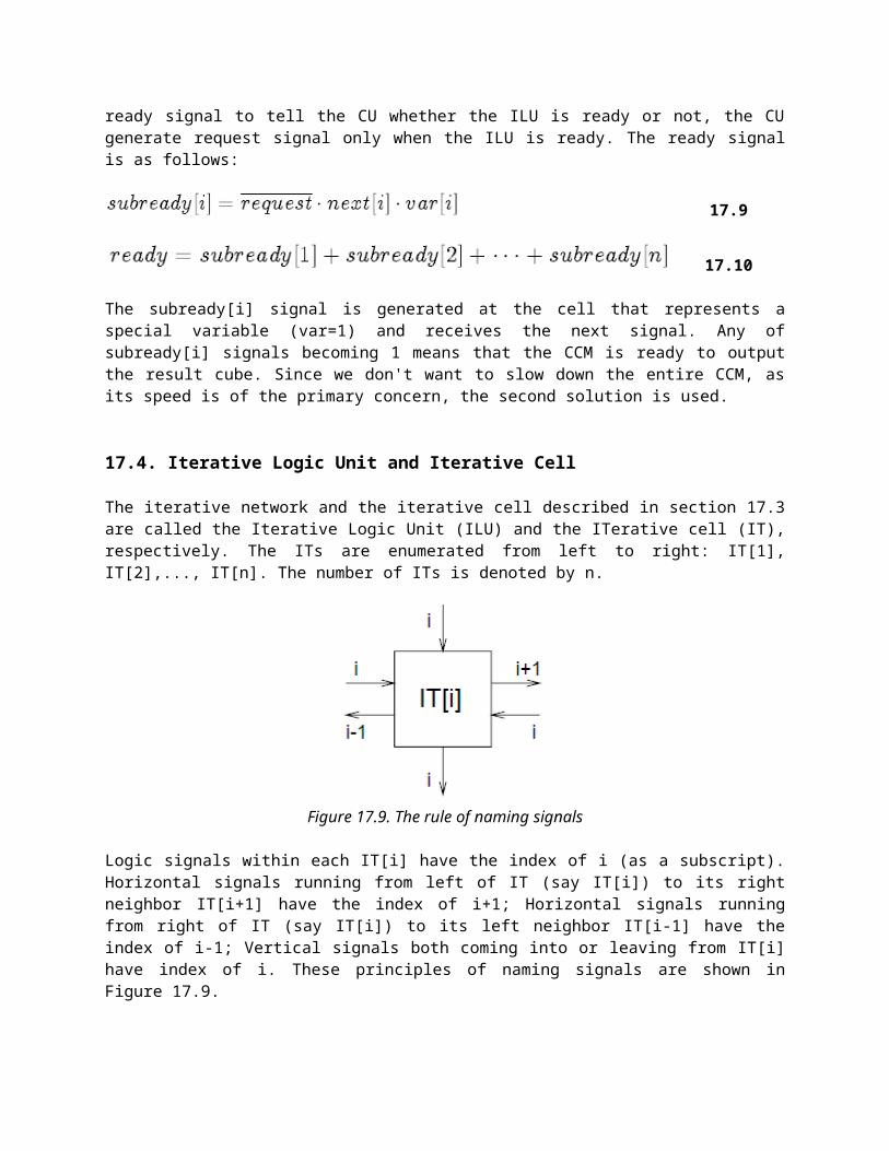
The iterative network and the iterative cell described in section 17.3 are called the Iterative Logic Unit (ILU) and the ITerative cell (IT), respectively. The ITs are enumerated from left to right: IT[1], IT[2],..., IT[n]. The number of ITs is denoted by n.

Figure 17.9. The rule of naming signals

Logic signals within each IT[i] have the index of i (as a subscript). Horizontal signals running from left of IT (say IT[i]) to its right neighbor IT[i+1] have the index of i+1; Horizontal signals running from right of IT (say IT[i]) to its left neighbor IT[i-1] have the index of i-1; Vertical signals both coming into or leaving from IT[i] have index of i. These principles of naming signals are shown in Figure 17.9.

17.4.1. Handling multi-valued variables

In the previous section, we just stated that one cell of IT processes only a single variable. Since one cell processing one variable with arbitrary number of possible values would be not practical, so in our design, one cell (IT) can process one binary variable. However, in addition, for processing variables with more than two possible values (the so-called multi-valued variables), multiple ITs are combined together to process a multi-valued variable.

Because the CCM is a hardware, when it has been realized, it has a fixed number of iterative cells. When we use the CCM to solve a problem, we can not always use all of its iterative cells. Sometimes, we just use part of it. Therefore, we need a signal vector to tell whether a given iterative cell is used by an

operation or not. This signal vector is called water[i] where i=1,2,….,n (w[i] for short). The signal w[i]=1 means that IT[i] is not used, and it should be transparent to all signals running horizontally (recall, that signals running horizontally are the signals running between cells, like the signal next).

Example 17.4. Assume a CCM with 4 iterative cells. For a given cube operation, only two iterative cells are needed. The corresponding signal water should be

We use multiple iterative cells to handle a multi-valued variable. We need a signal vector to tell where is the boundary of a multi-valued variable. This signal vector is right_edge[i] (re[i] for short), where i = 1,2,…..,n. The signal re[i] = 1 means that IT[i] is the right edge of a variable. If all variables are binary, then all bits of right_edge are 1's. Since one iterative cell processes two possible values of a variable, we can process a multi-valued variable with an even number of possible values.

Example 17.5. Assume a CCM with 6 iterative cells. For a given cube operation, there are 3 variables with 2, 4 and 6 possible values, respectively. Therefore the signal right_edge is

Since all iterative cells are used, so the signal water is 000000.

Take w[i] and re[i] into account, for handling multi-valued variables, the next signal is described now as:

17.11

which means that when the IT[i] is not used (w[i]=1), the iterative cell is transparent to the signal next. Otherwise, the next signal will propagate till the right edge of the first special variable that it will encounter.

Two more propagation signals carry and conf are used to combine multiple iterative cells to process multi-valued variables. Let us discuss first a simplified example that shows how to use these two signals. Next the general equations for these two signals will be derived after the example.

Example 17.6. Three iterative cells are combined together to process a pair of operand literals of a 6-valued variable as shown in Figure 3.10. The water and right_edge signals are also shown in the figure.

Now the problem is that no iterative cell receives all bits of operand cubes, then no single iterative cell can determine signal var of the variable by itself (the signal var represents whether the variable is a special variable or not). For a given OR_type cube operation, the signal var should be (Equation 17.5):

17.12

Since a single iterative cell processes just two possible values, then we can let them be:

Substituting Equations (17.13), (17.14) into (17.15) gives:

17.16

Comparing Equations (17.12) and (17.16), we know that the signal var is generated, and var = carry[4]. Please note that the signal var is always finally generated at the last cell of a variable.

All three cells that process the variable should know the signal var. For the last cell of the variable (IT[3] in this example), var[3] = carry[4]. All other cells that process the same variable receive the signal var through the propagation signal conf from its successive cell. In other words, the signal var is propagated back to the preceding cells through the iterative signal conf. This can be described by:

17.17

It can be seen that the signal carry propagates from left to right until the right edge of the variable in order to generate signal var of the variable. Then signal var is propagated back (from right to left) through signal conf (Equation 17.17). This propagation path is shown in Figure 17.10 by shadow big arrow.

Figure 17.10. Three iterative cells combined together to process a 6-valued variable

For the AND_type cube operation, we only need to change “+" to “." in the Equations (17.12) to (17.16).

Now we are ready to derive general formula for signals carry[i], conf[i] and var[i]. The IT[i] processes two possible values of a variable, then there are two partial relations in one iterative cell:

17.13

17.15

17.14

17.18

17.19

where a0[i] and a1[i] are two input bits from operand literal A, b0[i] and b1[i] are two input bits from operand literal B. For AND type relation, signal carry_and (signal carry for AND type relation) can be described as:

For OR type relation, signal carry_or (signal carry for OR type relation) can be described as:

Signal right_edge can be used to determine whether or not a given IT[i] is the first/last IT of a variable:

Because IT[1] is always the first IT of a variable, then

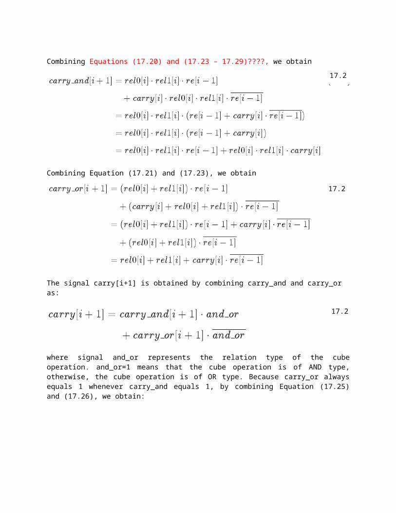
Combining Equations (17.20) and (17.23 – 17.29)????, we obtain

Combining Equation (17.21) and (17.23), we obtain

17.20

17.21

17.22

17.23

17.24

17.25

The signal carry[i+1] is obtained by combining carry_and and carry_or as:

where signal and_or represents the relation type of the cube operation. and_or=1 means that the cube operation is of AND type, otherwise, the cube operation is of OR type. Because carry_or always equals 1 whenever carry_and equals 1, by combining Equation (17.25) and (17.26), we obtain:

As shown in Example 17.6, signal conf can be generally described as:

Combining Equation (17.29) and (17.22), we obtain:

The signal var always comes from signal conf, which is:

If we also take the signal water into account, we obtain:

17.26

17.27

17.28

17.29

17.30

17.31

17.4.2. The design of an iterative cell

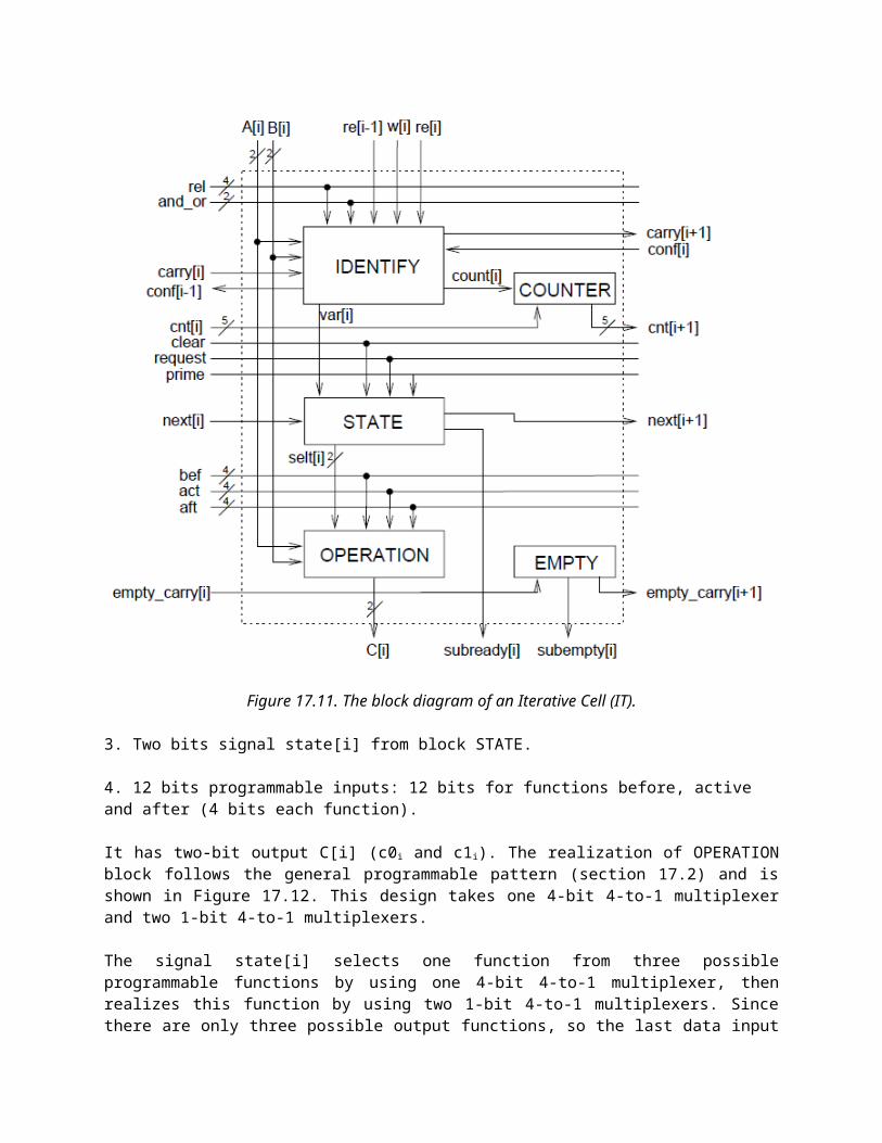
Now we know how iterative network works and how to combine multiple iterative cells to handle a multi-valued variable. This section will describe the details of the iterative cell that have not been discussed so far. The block diagram of one iterative cell is shown in Figure 17.11. As shown in the figure, one iterative cell can be divided into five blocks according to the function that they perform: IDENTIFY, STATE, OPERATION, COUNTER and EMPTY. All signals except the signals of COUNTER block in the figure were already discussed in the previous sections. The COUNTER block will be discussed in this section.

17.4.2.1. OPERATION block

The operation block is the combinational logic block B in Figure 17.5. This block creates bits of resultant cubes by performing the operation on bits of the argument cubes according to the state of IT. It takes the following inputs:

1. Two bits from operand literal A[i] (a0i, a1i).

2. Two bits from operand literal B[i] (b0i and b1i).

17.32

17.33

Figure 17.11. The block diagram of an Iterative Cell (IT).

3. Two bits signal state[i] from block STATE.

4. 12 bits programmable inputs: 12 bits for functions before, active and after (4 bits each function).

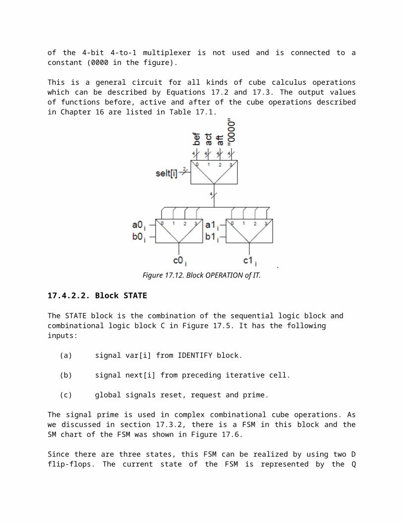
It has two-bit output C[i] (c0i and c1i). The realization of OPERATION block follows the general programmable pattern (section 17.2) and is shown in Figure 17.12. This design takes one 4-bit 4-to-1 multiplexer and two 1-bit 4-to-1 multiplexers.

The signal state[i] selects one function from three possible programmable functions by using one 4-bit 4-to-1 multiplexer, then realizes this function by using two 1-bit 4-to-1 multiplexers. Since there are only three possible output functions, so the last data input of the 4-bit 4-to-1 multiplexer is not used and is connected to a constant (0000 in the figure).

This is a general circuit for all kinds of cube calculus operations which can be described by Equations 17.2 and 17.3. The output values of functions before, active and after of the cube operations described in Chapter 16 are listed in Table 17.1.

.Figure 17.12. Block OPERATION of IT.

17.4.2.2. Block STATE

The STATE block is the combination of the sequential logic block and combinational logic block C in Figure 17.5. It has the following inputs:

(a) signal var[i] from IDENTIFY block.

(b) signal next[i] from preceding iterative cell.

(c) global signals reset, request and prime.

The signal prime is used in complex combinational cube operations. As we discussed in section 17.3.2, there is a FSM in this block and the SM chart of the FSM was shown in Figure 17.6.

Since there are three states, this FSM can be realized by using two D flip-flops. The current state of the FSM is represented by the Q outputs of these two flip-flops, denoted by state0[i] and state1[i]. The next state of the FSM is represented by D inputs of these two flip-flops, denoted by ex0 and ex1. This state machine can be described using the following formulas:

MISSING EQUATIONS.

The signal selt1[i] and selt0[i] can be described by:

17.39

17.40

17.34

These two equations indicate that signal selt[i] (selt0[i] and selt1[i]) is set to 01 to select active function for the ITs that are specific positions when ILU executes the complex combinational cube operation (like prime). The signal next[i+1] generated in this block is described by Equation (17.11).

IDENTIFY block

The IDENTIFY block is the combinational logic block A in Figure 17.5. The details of this block are fully discussed in section 3.4.1. The counter signal count generated in this block will be discussed in the next section, COUNTER block.

COUNTER block

The paper [31] shows that in addition to cube calculus operations presented in this book, the operation which take cubes as argument and return a number as a result is necessary. The simplest of such operation is calculating Hamming distance of two binary vectors. All such operation require the operation of counting. In this simplified machine, we introduce counting, but it is restricted only to very simple operation used in the pre-processing of cubes. This counting is done by COUNTER block.

The COUNTER block counts the number of specific variables which is used in pre-relation/pre-operation (see section 17.5). The signal count[i] equals 1 in the last IT of the specific variables. It can be described by:

17.41

The count[i] signal is generated in block IDENTIFY.

Figure 17.13. Counter.

The counter is realized by an iterative network. A 3-bit counter is shown in Figure 17.13. The COUNT block is just a cell of the iterative network of the counter. To minimize the necessary logic for the cell, the cell of the counter is based on the pseudo-random sequence generator. Figure 17.13 (a) shows a cell; and Figure 17.13(c) shows the whole picture of the counter. This iterative counter can generate a fixed sequence of 7 numbers which is shown in Figure 17.13(b) (number 000 is not used). Therefore, this counter can be used to count the number of 1's in signal vector x.

The count begins with all bits are 1's. As the bits are shifted, a series of unique numbers will be generated and they are shown in Figure 17.13(b). Since there must always be at least one bit equal to one in the pseudo-random counter, a k bits counter can count from 0 to 2 k-2. Therefore, a 3 bits counter can count from 0 to 6.

3 bits counter is sufficient for an ILU with 6 ITs. If all variables are binary, there are 6 specific positions at most. The counter must be able to signal 7 different numbers, to include the case where there are no specific positions. A decoder is needed to convert the output of the last cell of counter to a binary number.

EMPTY block

One of the main design objectives of the CCM design was not to generate empty cubes. In order to do this, in this design we simplified the previous designs from [15,17,18]. This led us to design the EMPTY block presented here. The role of this block is to generate signal empty to the control unit of the CCM informing whether the current resultant cube is a contradiction (empty cube) or not. This signal is used by the control unit of the CCM to remove empty cubes in the results, and makes the CCM not to generate empty cubes (see section 19.4??).

Figure 17.14. Iterative network used to generate empty signal

The empty signal is generated by a iterative network shown in Figure 17.14. The signal empty_carry[i] and subempty[i] are as follows:

17.42

17.43

The empty signal is as follows:

17.44

By comparing empty signal to carry signal, these equations are not hard to understand.

17.5. The architecture of the CCM

In our design, the cube calculus machine is a coprocessor to the host computer. The simplified block diagram of the CCM is shown in Figure 17.15; the thick arrow stands for data buses, and the thin arrow stand for control buses. As shown in the figure, the CCM communicates with the host computer through the input and the output FIFO. The ILU can take the input from register file and memory, and can write output to the register file, the memory, and the output FIFO. The ILU executes the cube operation under the control of Operation Control Unit (OCU). The Global Control Unit (GCU) controls all parts of the CCM and let them work together.

Figure 17.15. The simplified block diagram of the CCM

Since the design of the GCU depends on the design of the entire CCM, we will discuss the GCU in section 19.4 after the design of the CCM has been discussed in detail. In the next section, we will discuss the function of the OCU.

17.6. The Operation Control Unit (OCU)

The ILU executes cube operations under the control of the operation control unit (OCU) in our design; and the OCU is under the control of the GCU. The communication between the GCU and

OCU is very simple: when the CCM is ready to execute the cube operation, the GCU set the signal ilu_enable to 1 to tell the OCU to execute the cube operation; then the OCU controls the ILU to execute the cube operation; after the cube operation is done, the OCU set the signal ilu_done to 1 to tell the GCU that the cube operation is done. This is illustrated in Figure 17.16.

Figure 17.16. The communication between the GCU and the OCU

The algorithm of the CCM has been discussed in section 17.3.2. The state diagram of OCU is shown in Figure 17.17. Now let us take a look at these states.

Figure 17.17. The state diagram of the OCU

• State S0: This is the initial state of the OCU. The clear signal (see Figure 17.7) is set to 1. The clear signal is connected to all synchronous reset inputs of the D flip-flops that are used to realize the state machines inside ITs, therefore, all ITs are reset to state before.

If the signal ilu_enable is 1, then the OCU goes to state S1; otherwise, the OCU keeps in state S0.

When the CCM is used to calculate combinational cube operations (including complex combinational cube operations), the OCU keeps in state S0 because the GCU will keep the signal ilu_enable to be 0.

• State S1: The OCU let the ILU begin to execute the sequential cube operation by setting the signal init (the first next signal) to 1 in this state. After that, the OCU will wait for signals term (the last next signal) and ready. If signal term becomes 1, which means the cube operation is done, then the OCU goes to state S5. If signal ready becomes 1 and signal term keeps 0, then the OCU goes to state S2; otherwise (both signals keep 0), the OCU will keep in state S1.

• State S2: The OCU generates the first resultant cube by setting signal request to 1; and it also generates signals write_output to write the result out. The OCU will always go to state S3 from state S2.

• State S3: The OCU will wait for signals term and ready again. If signal term becomes 1, then the OCU goes to state S5; if signal ready becomes 1 and signal term keeps 0), then the OCU goes to state S4; otherwise (both signals keep 0), the OCU will keep in state S3.

• State S4: The OCU generates one resultant cube by setting signal request to 1; and it also generates signals write_output to write the result out. The OCU will always go to state S3 from this state.

• State S5: The OCU informs the GCU that the cube operation is done by setting the signal ilu_done to 1. The OCU will always go to state S0 from this state.

17.7. Pre-relation/Pre-operation

To explain the concept of pre-relation/pre-operation, let us take a look at the sharp operation again. The sharp operation is defined by Equations 16.12 and 16.13. It can be seen that we cannot use Equation 16.13 to carry out the operation unless two operand cubes satisfy

and . When , the operation ; when , the operation . and are called pre-relation of the sharp operation;

are called pre-operation of the sharp operation. It can be seen that the pre-operation is the output function when pre-relation is satisfied.

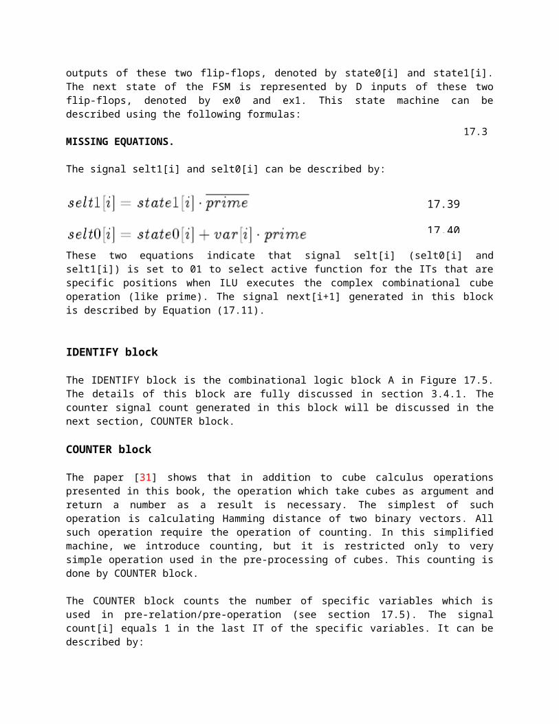
Table 17.2. Pre-relation and Pre-operation of the Cube Calculus Operations

Some cube operations which have pre-relation and pre-operation are listed in Table 17.2. The name, pre-relation and pre-operation of the operations are listed from left to right in the table, respectively. It can be seen that some cube operations have two pre-relations and pre-operations, such as the sharp and consensus operations.

As we discussed in section 17.4.2, the COUNT block can count the number of specific variables. In another words, it can count the number of the pairs of literals A i and Bi that satisfy the relation. If the relation (rel and and_or) are substituted by the pre-relation, the COUNT block can be used to count the number of the pairs of literals Ai and Bi that satisfy the pre-relation.

Example 17.7. For the pre-relation , we can count the number (denoted by k) of the

pairs of literals Ai and Bi that satisfy . If k > 0, then , otherwise (k=0), .

The pre-relation can be represented by partial pre-relation (prel), partial pre-relation type (pand_or), pre-relation compare type (pcmp) and pre-relation compare value (pval).

Example 17.8. For the pre-relation shown in Example 17.7, prel is ; pand_or is and; pcmp is “>"; and pval is 0 ( is the relation of the crosslink operation, so prel and pand_or are the same as rel and and_or of the crosslink operation, respectively).

The pre-operations listed in Table 17.2 are bitwise functions. The decomposed pre-relations and pre-operations of the sharp/disjoint sharp and consensus operations are listed in Table 17.3. The crosslink operation cannot be decomposed in this way (It needs two carry signals to compare the degrees of two operand cubes; but this simplified design of the CCM has only one carry signal, see [15]). Each row of the table describes one pair of pre-relation and pre-operation.

Table 17.3. Decomposed Pre-relation and Pre-operation of the Cube Operations

The encoded pre-relations and pre-operations of the sharp/disjoint sharp and consensus operations are listed in Table 17.4. The prel and pre-operation (poper) are decoded by their output values. The encoding of pand_or is the same as and_or. The encoding of pcmp is as follows: “<" --- 00, “=" --- 01 and “>" --- 10. Each row of the table describes one pair of pre-relation and pre-operation.

Table 17.4. Encoded Pre-relation and Pre-operation of the Cube Operations

For realizing pre-relation/pre-operation, the ILU is modified as shown in Figure 17.18. Please note that only the modified part is shown in the figure. This design is very straightforward. In this design, a cube operation can have at most two pairs of pre-relation/pre-operation, and all pre-operations should be combinational operations, which means that the operation can be described as a bitwise function. Thus the signals prel, pand_or, pcmp, pval and poper shown in the figure have a suffix 1 or 2, which corresponds to the first or the second pair of the pre-relation/pre-operation, respectively. All input signals come from the registers (see section 19.2.3).

Figure 17.18. Realization of Pre-relation/Pre-operation

The signal prel_sel (having 2 bits) is generated by the GCU (see section 19.4). When the CCM executes the first pre-relation/pre-operation, the signal prel_sel = 00; when the CCM executes the second pre-relation/pre-operation, the signal prel_sel = 01; otherwise, the signal prel_sel = 10.

The only output signal prel_res is the result of pre-relation. When prel_res=1, the pre-relation is satisfied, otherwise, the pre-relation is not satisfied. This signal is used by the GCU (see section 19.4).

If prel_sel=00 or 01, and all ITs of the ILU are in before state, then the cube operation is evaluated according to the function poper1 or poper2, respectively.

Let us observe that among combinational cube operations that have pre/relation/pre-operation, there exists certain subset operations, like intersection and cofactor operations, can be characterized by the following:

• These operations only have one pair of pre-relation/pre-operation, and the result of pre-operation is always an empty cube.

• These operations can be always carried out by following the basic equation of the operation without checking the pre-relation. After that the EMPTY blocks will check whether the result is an empty cube or not.

• These operations can be carried out using pre-relation/pre-operation, but it will take more time to execute this kind of operations because the GCU will go through more states to check the pre-relation (see section 19.4).

Based on these observations, this kind of operations will be carried out without using pre-relation/pre-operation in this book.

17.8. Questions and problems to solve.