Embed Size (px)
Citation preview

Week 10: Markov Models I
Marcelo Coca Perraillon
University of ColoradoAnschutz Medical Campus
Cost-Effectiveness AnalysisHSMP 6609
20120
1 / 34

Outline
Elements of Markov models
Example: HIV transitions
State transition diagrams
Adding costs and benefits
Simulating the transitions of a cohort
Half-cycle correction
The memoryless property of cohort models
Markov models as “trees”
When should we use Markov models?
2 / 34
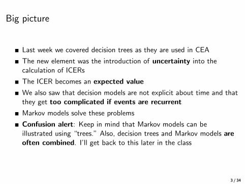
Big picture
Last week we covered decision trees as they are used in CEA
The new element was the introduction of uncertainty into thecalculation of ICERs
The ICER becomes an expected value
We also saw that decision models are not explicit about time and thatthey get too complicated if events are recurrent
Markov models solve these problems
Confusion alert: Keep in mind that Markov models can beillustrated using “trees.” Also, decision trees and Markov models areoften combined. I’ll get back to this later in the class
3 / 34
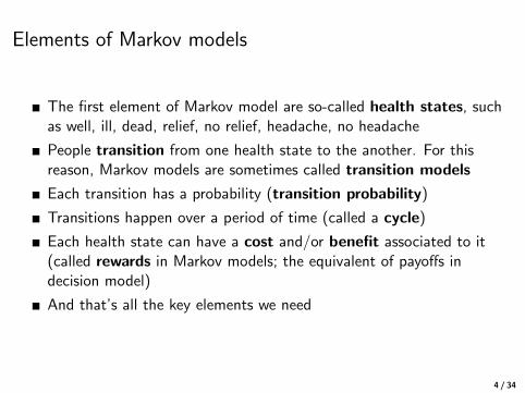
Elements of Markov models
The first element of Markov model are so-called health states, suchas well, ill, dead, relief, no relief, headache, no headache
People transition from one health state to the another. For thisreason, Markov models are sometimes called transition models
Each transition has a probability (transition probability)
Transitions happen over a period of time (called a cycle)
Each health state can have a cost and/or benefit associated to it(called rewards in Markov models; the equivalent of payoffs indecision model)
And that’s all the key elements we need
4 / 34

Example
We;’ll use a now-classic example from your textbook and Briggs et al(2006) (available on Canvas)
Two therapeutical strategies for HIV: zidovudine monotherapy andzidovudine in combination with lamivudine (for simplicity,“monotherapy” versus “combination” therapy)
Four possible health states, some of them depending on CD4 counts:
1 State A: CD4 from 200 to 500 (best)2 State B: CD4 less than 200 (not so good)3 State C: AIDS (bad)4 State D: Death (very bad)
Cycle length is one year
We can illustrate the states and all possible transitions with a statetransition diagram
5 / 34
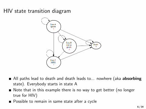
HIV state transition diagram
All paths lead to death and death leads to... nowhere (aka absorbingstate). Everybody starts in state A
Note that in this example there is no way to get better (no longertrue for HIV)
Possible to remain in same state after a cycle6 / 34

Transition probabilities (matrix)
Read them from left to right: probability of transitioning from C toDeath is 0.25
Note that combo therapy has better outcomes. To be precise,combo therapy’s risk is reduced by about half (0.509)
See Excel file for actual probabilities
7 / 34

Transition probabilities (matrix)
Note that probabilities must up to one (horizontally):0.721 + 0.202 + 0.067 + 0.01 = 1 (always check!!)
Note that this implies that we always must “account” for peopletransitioning. They can either stay in the same state or they must gosomewhere in each cycle
Similar to decision trees, probabilities are exhaustive and mutuallyexclusive
Note death. Death is final. A person who gets there stays there8 / 34
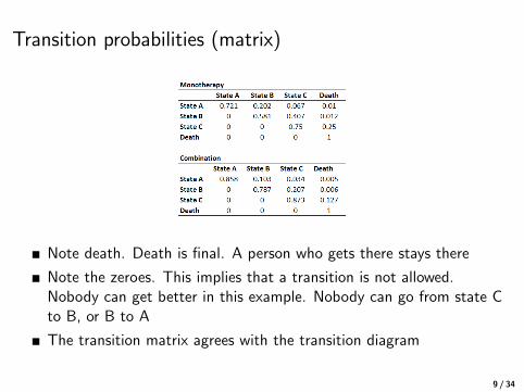
Transition probabilities (matrix)
Note death. Death is final. A person who gets there stays there
Note the zeroes. This implies that a transition is not allowed.Nobody can get better in this example. Nobody can go from state Cto B, or B to A
The transition matrix agrees with the transition diagram
9 / 34

Where do probabilities come from?
As with decision models, probabilities come from clinical trials,observational data, meta-analyses, expert panels, surveys...
Note that we could have used a decision tree instead
More precisely, a recursive decision tree with one tree per year but itwould be too complicated (the “bushy” tree problem)
Now we need to add rewards (i.e. payoffs)
10 / 34

The language of trees vs Markov modelsNow probabilities are called transition probabilities. Now events arestates. There are no “branches;” but going from one state to anotherhas a probability
Now there is time: everything happens in a cycle, which can be 1week, 1 year, etc
Payoffs are now rewards which are part of each state (more in asecond)
Long history in statistics. Introduced by Andrew Markov in 1906
Careful when googling. We are covering Markov or transitionmodels, which are examples of a Markov process. But many thingscome under the name “Markov process.” Same with decision trees.Decision trees in machine learning have nothing to do withdecision trees in decision theory. They are actually regressiontrees, not decision trees. The similarity is that in both cases you candraw something that sort of looks like a tree. That’s where thesimilarity ends
11 / 34

Costs
We will first do a cost analysis (we will add life years later)
The HIV study collected health care, community, and medicationcosts
Drug costs: zidovudine (£2,278); lamivudine (£2,086); combination(£4364)
Cost per state (health care and community): A: £2756; B: £3052 C:£9007; D: £0
Costs are per cycle (i.e. year)
Keep in mind a couple of things: combination therapy is moreexpensive but also more effective (first quadrant in thecost-effectiveness plane)
The worse the state the higher the costs, but once in state “death”there is no cost. If end-of-life costs were significant, we could haveadded another state
12 / 34
“Solving” Markov models
We now have all ingredients: health states, transition probabilities,and rewards for each cycle
“Solving” the Markov model means that we will simulate what wouldhappen to a group (cohort) of people over time (that’s why they arecalled cohort models sometimes)
We will then calculate expected costs
In this example, we will simulate the transitions of 1,000 patients ineach type of therapy over 20 years
Why 20 years? Because most of our population won’t live longer. Soit’s really a lifetime time horizon
Pay attention! It’s actually very easy but it’s also very easy to getconfused
13 / 34
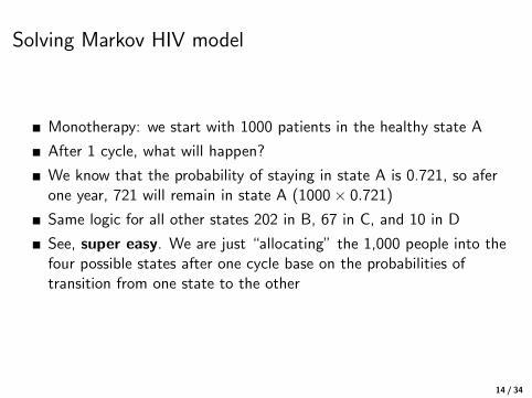
Solving Markov HIV model
Monotherapy: we start with 1000 patients in the healthy state A
After 1 cycle, what will happen?
We know that the probability of staying in state A is 0.721, so aferone year, 721 will remain in state A (1000 × 0.721)
Same logic for all other states 202 in B, 67 in C, and 10 in D
See, super easy. We are just “allocating” the 1,000 people into thefour possible states after one cycle base on the probabilities oftransition from one state to the other
14 / 34

Solving Markov HIV model
Now we need to repeat the process for the next cycle
Of the 721 in state A, how many will stay in A? 520 (0.721 × 721)
How many in B? We need to take into account that some will movefrom A to B but also that some in B will stay in B:721 × 0.202 + 202 × 0.581 = 263 (here is where you are likely tomake mistakes)
Easier to see it graphically
15 / 34

Transition probabilities
16 / 34
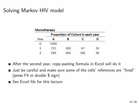
Solving Markov HIV model
After the second year, copy-pasting formula in Excel will do it
Just be careful and make sure some of the cells’ references are “fixed”(press F4 or double $ sign)
See Excel file for this lecture
17 / 34

Big picture
We start with a group of patients (the number doesn’t matter, wecould use 1 person, but you need to use the same number of peoplein both or do it by person)
Cycle by cycle, we transition them to different health states
That’s it. Really, that’s all. We have simulated disease progression
Note that we are transitioning a group of patients. We are NOTfollowing each patient (more on this later as it becomes veryimportant)
We are moving a cohort into the simulation. Each cycle theyaccumulate costs and life
18 / 34
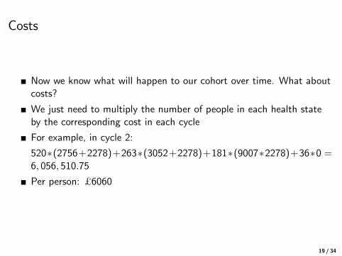
Costs
Now we know what will happen to our cohort over time. What aboutcosts?
We just need to multiply the number of people in each health stateby the corresponding cost in each cycle
For example, in cycle 2:
520∗(2756+2278)+263∗(3052+2278)+181∗(9007∗2278)+36∗0 =6, 056, 510.75
Per person: £6060
19 / 34
Life years gained
We are simulating 20 years of life for these patients
Some of them die (for example, 10 in the first cycle, 26 in the second)
We can therefore calculate life years in each cycle
In the first cycle, 10 people died but 990 were alive so these “alive”people accumulated 990 life years in the first cycle
In the second cycle, 520 + 263 + 181 = 964 were alive, so theyaccumulated another 964 years of life
We do the same for each cycle
At the end of the 20 cycles, we add up all the years of life over the 20years
20 / 34

We can plot a survival curve
21 / 34

Half-cycle correction
Why didn’t we give any life years “credit” to those who died duringeach cycle?
Because we essentially assumed that people died at the start of thecycle
But we should take into account that patients die at different times;otherwise, we underestimate costs and benefits
Not a big problem if we do the same in both treatments (the shorterthe cycles the less of a problem)
The best solution (the unbiased solution) is to assume that patientsdie in the middle of the cycle
This is a result of assuming that patients die (uniformly during theyear. That is, dying follows a uniform distribution. Or said anotherway, the probability of death is the same every day during the year
22 / 34

Half-cycle correction
Check out the formula in the Excel example
We add half the time of those who died during the year
We won’t worry about the half-cycle correction for the rest of thesemester
23 / 34

CEA
We now have costs and life years gain over the time horizon
We need to repeat the same simulation for another cohort for thecombination group (homework)
The way I worked out this example, we need to simulate 1,000patients in the combination group
Not really necessary. We could calculate costs and benefits for anynumber or do it by person
After calculating costs and benefits for both groups, we can obtainthe ICER
24 / 34
What about QALYs and other features of CEAs?
Note that adjusting for quality (i.e. preferences) is straightforward
Each health state would have a preference score (the number between0 and 1) associated with it
We just multiply the score by the time spent in each year
Discounting is easy too: we have costs and benefits per cycle so wejust need to bring them into the present
Note that with Markov models we can go from intermediate to finaloutcomes since we’re modeling disease progression
Note that we’re ignoring something important in this basic example:people getting older but their chance of dying is not changing
Easy to incorporate: increase the chances of dying of other causes bycycle (next class)
25 / 34
Department of Pesky Things that CauseUnnecessary Confusion
Be careful when you read CEA papers
1) Markov models are depicted using transition diagrams, but theycan also be depicted using something that looks like a tree, but it’snot a decision tree
2) Decision trees and Marvok models can be combined
You can have a Markov models within a decision tree
26 / 34

Markov models depicted as trees
27 / 34

Markov models inside decision trees
Some parts of a decision tree could be calculated using Markovmodels
28 / 34
Big picture
Markov models and decision models are not that different
We have changed the language because decision trees and Markovmodels have different origins
Health states could be represented by a branch in a decision tree
In the migraine example, health states could be relief, no relief, norecurrence, recurrence, hospitalization...
The main difference is the introduction of time in the form of cyclesand that recurrent events are easily modeled
In the migraine example, an appropriate cycle could be a day or aweek
29 / 34

The memoryless property or the Markov assumption
One limiting assumption of cohort Markov models is that transitionsto a state do not depend on the past or the time a patient hasbeen in a state
In other words, once in a cycle, there is no “memory” of the past
In many cases, how long a patient stays in a state affects the chancesof an outcome
For example, a person experiencing his third bout of depression hashigher chances of worse outcomes
There are ways to fix this limitation: adding additional transitionstates (second, third depression episode) and/or making transitionprobabilities conditional on past events
In general, this can be an important limitation and we will seeextensions
30 / 34
When should we use Markov models?
When events are recurrent
When we want to model the “natural history” of the disease
Long time horizon: we want to go for intermediate outcomes to finaloutcomes
When life years or QALYs are outcomes of interest
Markov models are the most commonly used tool in costeffectiveness
31 / 34

Cycle length and some limitations
Important: We haven’t talked much about this but choosing avalid cycle length matters
Ideally we want a cycle length in which two events usually do nothappen
Cohort Markov models are not good for modeling infectious diseases:the probability of infection depends on the number of people infectedand (herd immunity)
Cohort models modeling a group transitioning, but can’t follow aperson
Next class we will see some extensions and tricks we can do to addmore flexibility to Markov models but they do have limitations
We will also cover a basic model of infectious disease using differenttools but also using Excel
32 / 34

Summary
Markov models allow us to model complex diseases
Markov models better incorporate time and disease progression
Simulating cohort models is easy
As with decision analysis, the hard part is to come up with a modelthat isolates the key elements that need to be considered –that’s noteasy
There are extensions to Markov models that are better for someproblems (next week)
33 / 34

Next class
More examples
Incorporating time dependency
Adding memory to the memoryless model
Temporary states
Other type of models in CEA
34 / 34