Embed Size (px)
Citation preview
Week 3 & 4Randomized Blocks, Latin Squares,
and Related DesignsJoslin Goh
Simon Fraser University
Week 3 & 4Randomized Blocks, Latin Squares, and Related Designs – p. 1/81
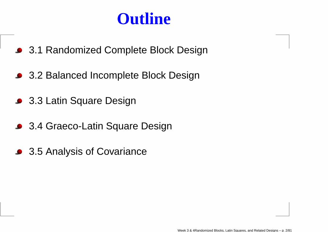
Outline
3.1 Randomized Complete Block Design
3.2 Balanced Incomplete Block Design
3.3 Latin Square Design
3.4 Graeco-Latin Square Design
3.5 Analysis of Covariance
Week 3 & 4Randomized Blocks, Latin Squares, and Related Designs – p. 2/81
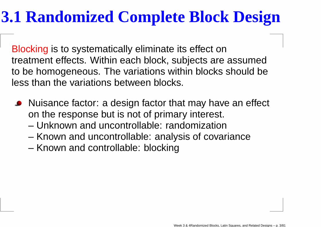
3.1 Randomized Complete Block Design
Blocking is to systematically eliminate its effect ontreatment effects. Within each block, subjects are assumedto be homogeneous. The variations within blocks should beless than the variations between blocks.
Nuisance factor: a design factor that may have an effecton the response but is not of primary interest.– Unknown and uncontrollable: randomization– Known and uncontrollable: analysis of covariance– Known and controllable: blocking
Week 3 & 4Randomized Blocks, Latin Squares, and Related Designs – p. 3/81

Examples
a. Four training processes for IQ Score, 16 Students, eachof 4 students are from the same department.
b. Test 3 crop varieties on 5 fields.
c. An industrial engineer is conducting an experiment oneye focus time. He is interested in the effect of thedistance of the object from the eye on the focus time.Four different distances are of interest. He has fivesubjects available for the experiment.
Week 3 & 4Randomized Blocks, Latin Squares, and Related Designs – p. 4/81
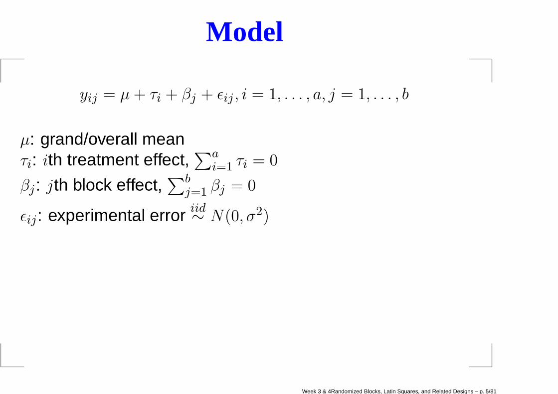
Model
yij = µ+ τi + βj + ǫij , i = 1, . . . , a, j = 1, . . . , b
µ: grand/overall meanτi: ith treatment effect,
∑ai=1 τi = 0
βj: jth block effect,∑b
j=1 βj = 0
ǫij: experimental error iid∼ N(0, σ2)
Week 3 & 4Randomized Blocks, Latin Squares, and Related Designs – p. 5/81

Estimates
yij = µ+ τi + βj + rij
Week 3 & 4Randomized Blocks, Latin Squares, and Related Designs – p. 6/81
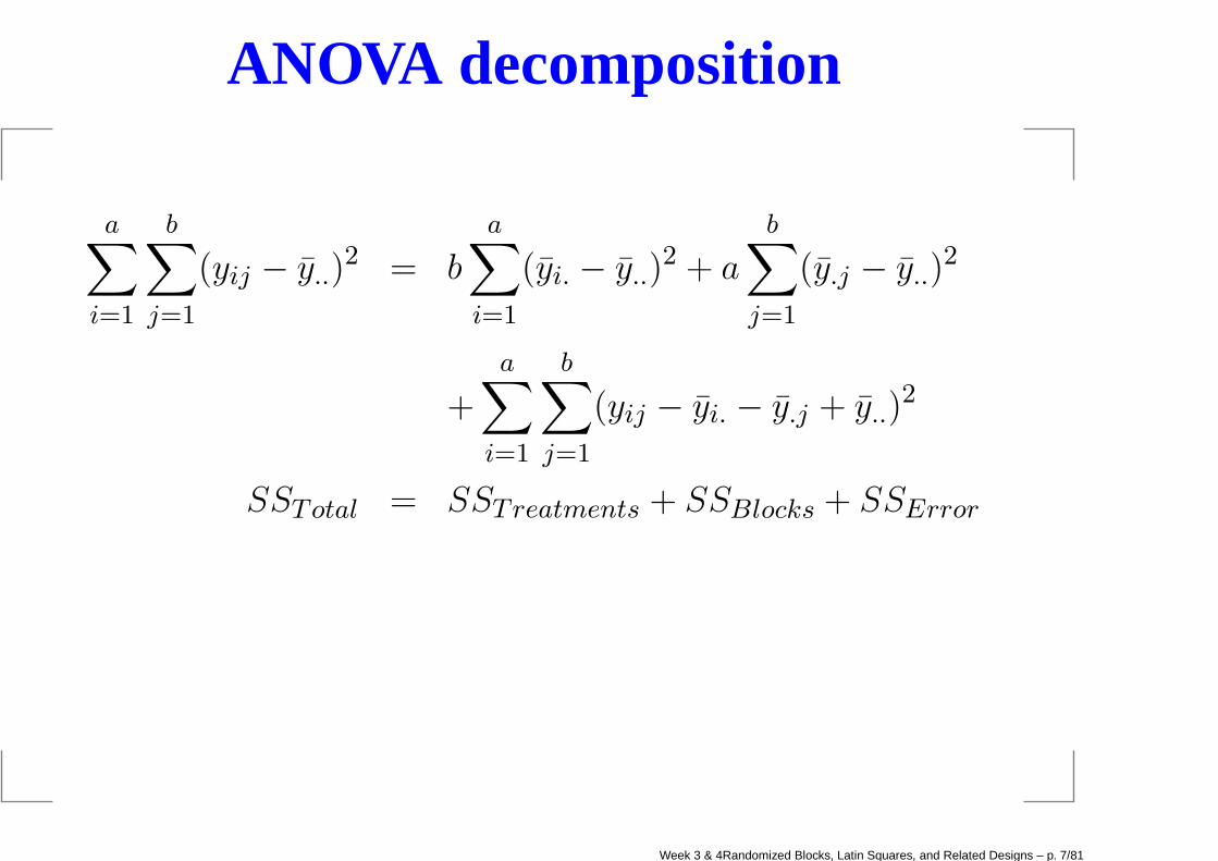
ANOVA decomposition
a∑
i=1
b∑
j=1
(yij − y..)2 = b
a∑
i=1
(yi. − y..)2 + a
b∑
j=1
(y.j − y..)2
+
a∑
i=1
b∑
j=1
(yij − yi. − y.j + y..)2
SSTotal = SSTreatments + SSBlocks + SSError
Week 3 & 4Randomized Blocks, Latin Squares, and Related Designs – p. 7/81
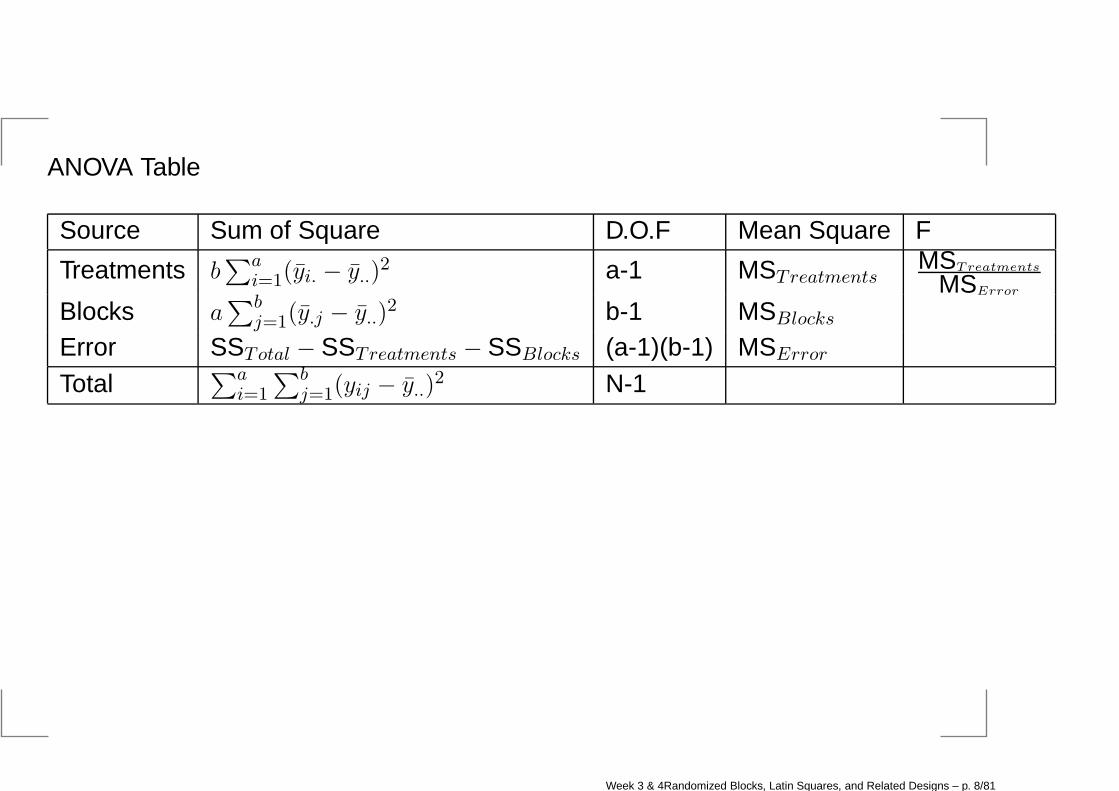
ANOVA Table
Source Sum of Square D.O.F Mean Square F
Treatments b∑a
i=1(yi. − y..)2 a-1 MSTreatments
MSTreatments
MSError
Blocks a∑b
j=1(y.j − y..)2 b-1 MSBlocks
Error SSTotal − SSTreatments − SSBlocks (a-1)(b-1) MSError
Total∑a
i=1
∑bj=1(yij − y..)
2 N-1
Week 3 & 4Randomized Blocks, Latin Squares, and Related Designs – p. 8/81
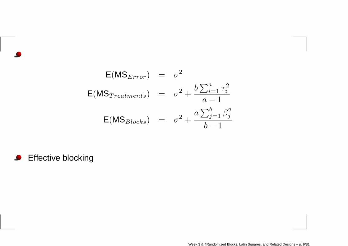
E(MSError) = σ2
E(MSTreatments) = σ2 +b∑a
i=1 τ2i
a− 1
E(MSBlocks) = σ2 +a∑b
j=1 β2j
b− 1
Effective blocking
Week 3 & 4Randomized Blocks, Latin Squares, and Related Designs – p. 9/81
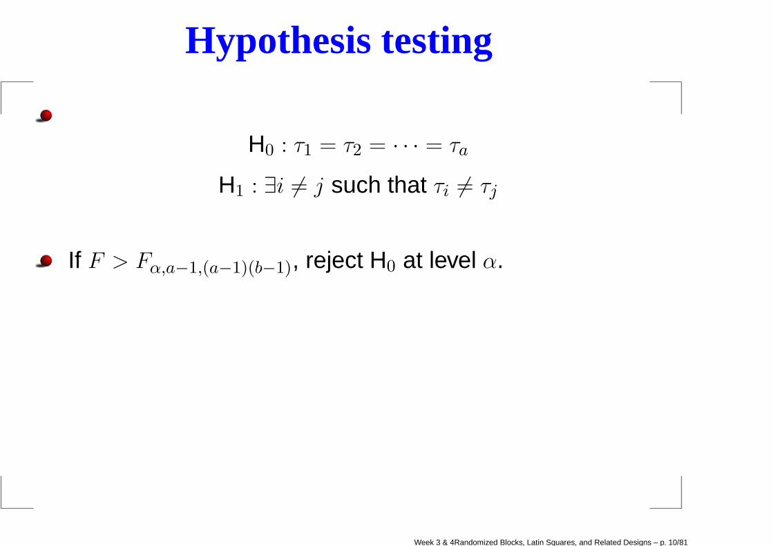
Hypothesis testing
H0 : τ1 = τ2 = · · · = τa
H1 : ∃i 6= j such that τi 6= τj
If F > Fα,a−1,(a−1)(b−1), reject H0 at level α.
Week 3 & 4Randomized Blocks, Latin Squares, and Related Designs – p. 10/81
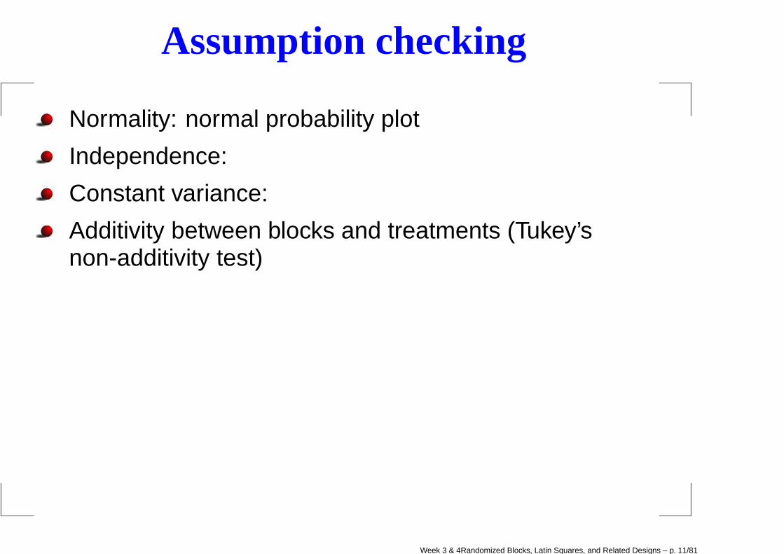
Assumption checking
Normality: normal probability plot
Independence:
Constant variance:
Additivity between blocks and treatments (Tukey’snon-additivity test)
Week 3 & 4Randomized Blocks, Latin Squares, and Related Designs – p. 11/81
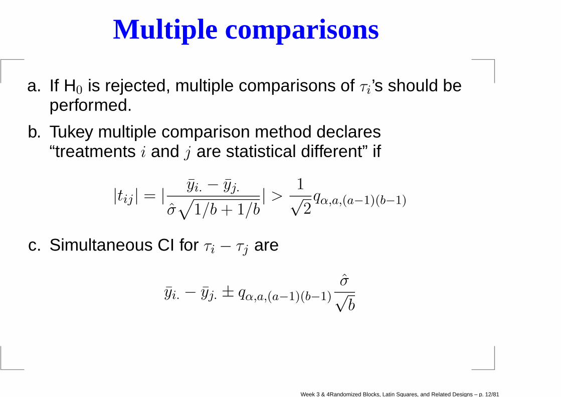
Multiple comparisons
a. If H0 is rejected, multiple comparisons of τi’s should beperformed.
b. Tukey multiple comparison method declares“treatments i and j are statistical different” if
|tij | = | yi. − yj.
σ√
1/b+ 1/b| > 1√
2qα,a,(a−1)(b−1)
c. Simultaneous CI for τi − τj are
yi. − yj. ± qα,a,(a−1)(b−1)σ√b
Week 3 & 4Randomized Blocks, Latin Squares, and Related Designs – p. 12/81

Example of Penicillin
Comparison of four variants of a penicillin product process
It was known that an important raw material, corn steep liquor, was quitevariable. Each blend of corn steep liquor is sufficient for four runs. Theexperiment was protected from extraneous unknown sources of bias byrunning the treatments in random order within each block.
Block Treatment Block
(blend of corn steep liquor) A B C D average
blend 1 89(1) 88(3) 97(2) 94(4) 92
blend 2 84(4) 77(2) 92(3) 79(1) 83
blend 3 81(2) 87(1) 87(4) 85(3) 85
blend 4 87(1) 92(3) 89(2) 84(4) 88
blend 5 79(3) 81(4) 80(1) 88(2) 82
Treatment Average 84 85 89 86 86=Grand Average
Week 3 & 4Randomized Blocks, Latin Squares, and Related Designs – p. 13/81
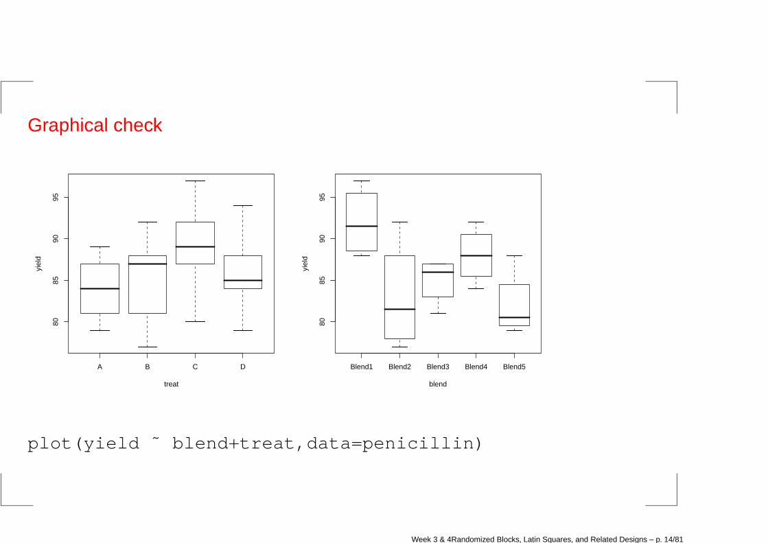
Graphical check
A B C D
8085
9095
treat
yiel
d
Blend1 Blend2 Blend3 Blend4 Blend5
8085
9095
blend
yiel
d
plot(yield ˜ blend+treat,data=penicillin)
Week 3 & 4Randomized Blocks, Latin Squares, and Related Designs – p. 14/81
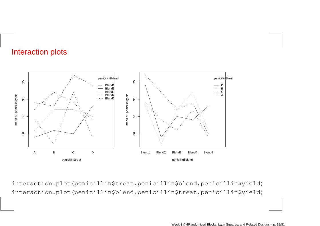
Interaction plots
8085
9095
penicillin$treat
mea
n of
pen
icill
in$y
ield
A B C D
penicillin$blend
Blend1Blend5Blend3Blend4Blend2
8085
9095
penicillin$blend
mea
n of
pen
icill
in$y
ield
Blend1 Blend2 Blend3 Blend4 Blend5
penicillin$treat
DBCA
interaction.plot(penicillin$treat,penicillin$blend, penicillin$yield)
interaction.plot(penicillin$blend,penicillin$treat, penicillin$yield)
Week 3 & 4Randomized Blocks, Latin Squares, and Related Designs – p. 15/81
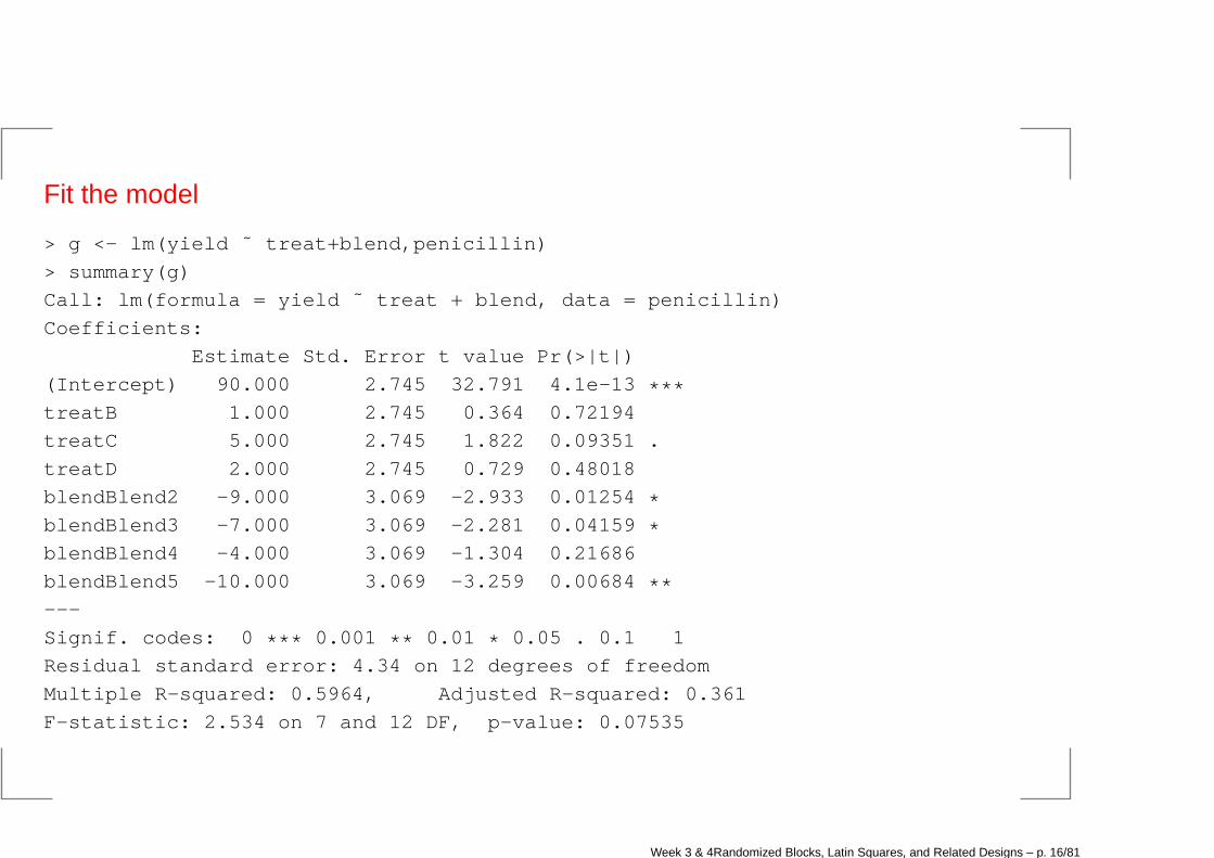
Fit the model
> g <- lm(yield ˜ treat+blend,penicillin)
> summary(g)
Call: lm(formula = yield ˜ treat + blend, data = penicillin)
Coefficients:
Estimate Std. Error t value Pr(>|t|)
(Intercept) 90.000 2.745 32.791 4.1e-13 ***treatB 1.000 2.745 0.364 0.72194
treatC 5.000 2.745 1.822 0.09351 .
treatD 2.000 2.745 0.729 0.48018
blendBlend2 -9.000 3.069 -2.933 0.01254 *blendBlend3 -7.000 3.069 -2.281 0.04159 *blendBlend4 -4.000 3.069 -1.304 0.21686
blendBlend5 -10.000 3.069 -3.259 0.00684 **---
Signif. codes: 0 *** 0.001 ** 0.01 * 0.05 . 0.1 1
Residual standard error: 4.34 on 12 degrees of freedom
Multiple R-squared: 0.5964, Adjusted R-squared: 0.361
F-statistic: 2.534 on 7 and 12 DF, p-value: 0.07535
Week 3 & 4Randomized Blocks, Latin Squares, and Related Designs – p. 16/81
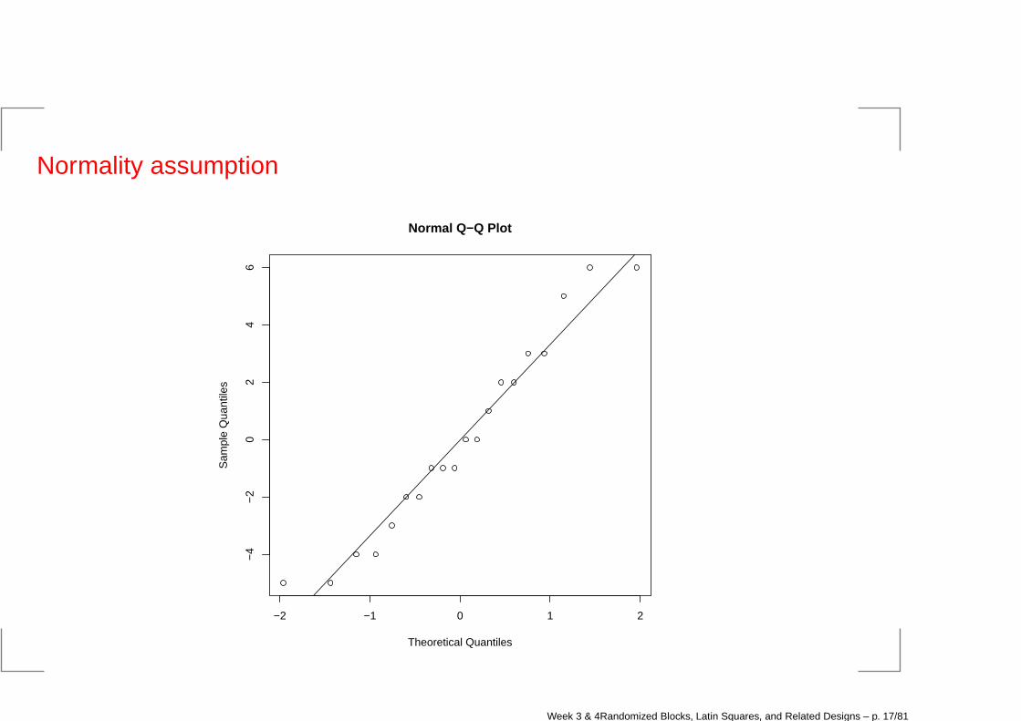
Normality assumption
−2 −1 0 1 2
−4
−2
02
46
Normal Q−Q Plot
Theoretical Quantiles
Sam
ple
Qua
ntile
s
Week 3 & 4Randomized Blocks, Latin Squares, and Related Designs – p. 17/81
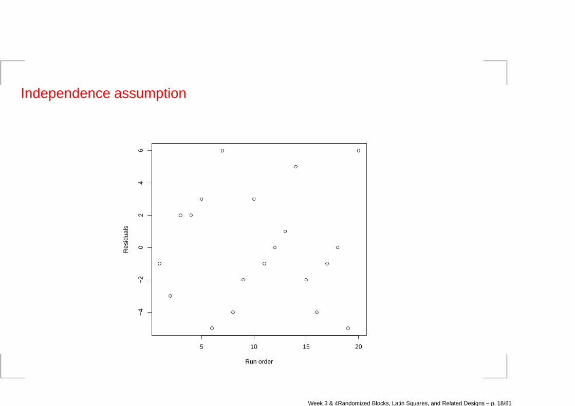
Independence assumption
5 10 15 20
−4
−2
02
46
Run order
Res
idua
ls
Week 3 & 4Randomized Blocks, Latin Squares, and Related Designs – p. 18/81
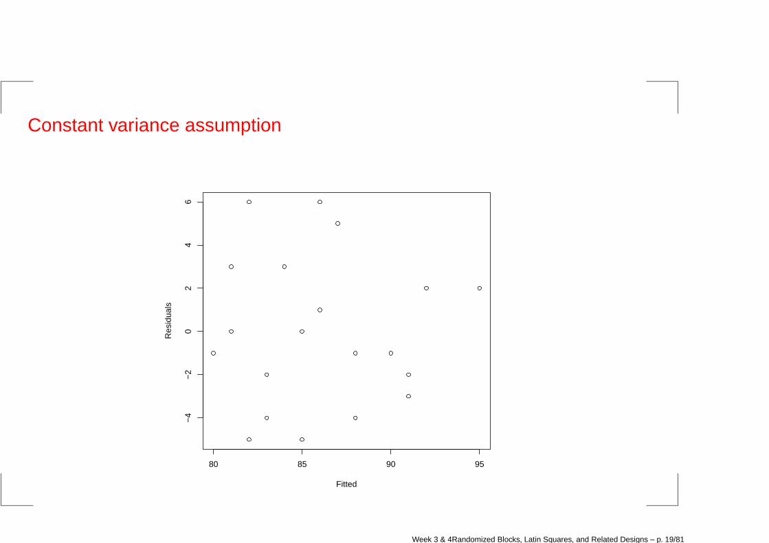
Constant variance assumption
80 85 90 95
−4
−2
02
46
Fitted
Res
idua
ls
Week 3 & 4Randomized Blocks, Latin Squares, and Related Designs – p. 19/81
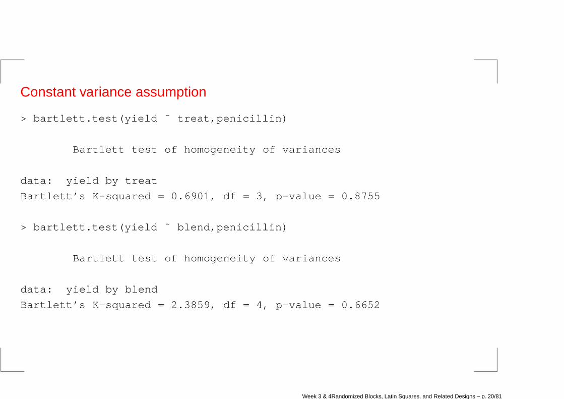
Constant variance assumption
> bartlett.test(yield ˜ treat,penicillin)
Bartlett test of homogeneity of variances
data: yield by treat
Bartlett’s K-squared = 0.6901, df = 3, p-value = 0.8755
> bartlett.test(yield ˜ blend,penicillin)
Bartlett test of homogeneity of variances
data: yield by blend
Bartlett’s K-squared = 2.3859, df = 4, p-value = 0.6652
Week 3 & 4Randomized Blocks, Latin Squares, and Related Designs – p. 20/81
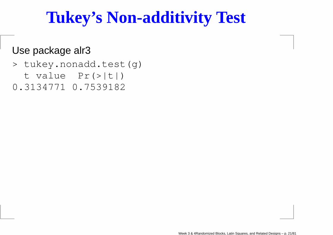
Tukey’s Non-additivity Test
Use package alr3> tukey.nonadd.test(g)
t value Pr(>|t|)0.3134771 0.7539182
Week 3 & 4Randomized Blocks, Latin Squares, and Related Designs – p. 21/81
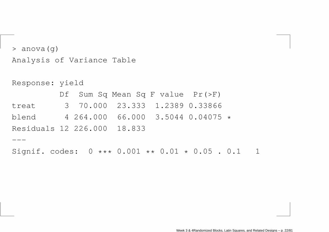
> anova(g)
Analysis of Variance Table
Response: yield
Df Sum Sq Mean Sq F value Pr(>F)
treat 3 70.000 23.333 1.2389 0.33866
blend 4 264.000 66.000 3.5044 0.04075 *Residuals 12 226.000 18.833
---
Signif. codes: 0 *** 0.001 ** 0.01 * 0.05 . 0.1 1
Week 3 & 4Randomized Blocks, Latin Squares, and Related Designs – p. 22/81
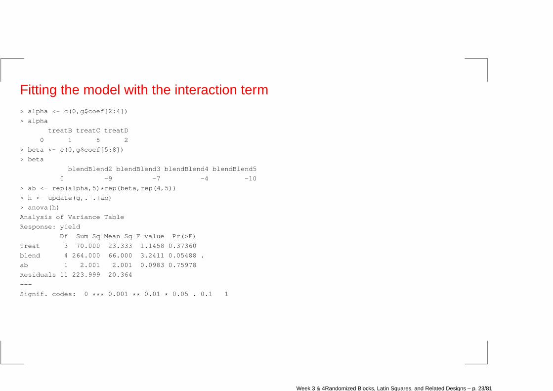
Fitting the model with the interaction term> alpha <- c(0,g$coef[2:4])
> alpha
treatB treatC treatD
0 1 5 2
> beta <- c(0,g$coef[5:8])
> beta
blendBlend2 blendBlend3 blendBlend4 blendBlend5
0 -9 -7 -4 -10
> ab <- rep(alpha,5) * rep(beta,rep(4,5))
> h <- update(g,.˜.+ab)
> anova(h)
Analysis of Variance Table
Response: yield
Df Sum Sq Mean Sq F value Pr(>F)
treat 3 70.000 23.333 1.1458 0.37360
blend 4 264.000 66.000 3.2411 0.05488 .
ab 1 2.001 2.001 0.0983 0.75978
Residuals 11 223.999 20.364
---
Signif. codes: 0 *** 0.001 ** 0.01 * 0.05 . 0.1 1
Week 3 & 4Randomized Blocks, Latin Squares, and Related Designs – p. 23/81
Multiple comparisons
Fisher’s LSD (“Least Significant Difference”)
Bonferroni method
Tukey method
Week 3 & 4Randomized Blocks, Latin Squares, and Related Designs – p. 24/81
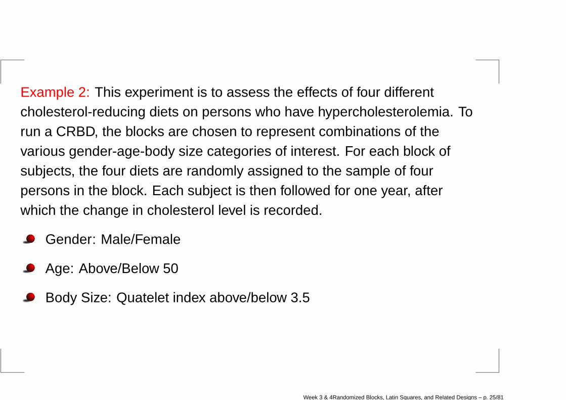
Example 2: This experiment is to assess the effects of four differentcholesterol-reducing diets on persons who have hypercholesterolemia. Torun a CRBD, the blocks are chosen to represent combinations of thevarious gender-age-body size categories of interest. For each block ofsubjects, the four diets are randomly assigned to the sample of fourpersons in the block. Each subject is then followed for one year, afterwhich the change in cholesterol level is recorded.
Gender: Male/Female
Age: Above/Below 50
Body Size: Quatelet index above/below 3.5
Week 3 & 4Randomized Blocks, Latin Squares, and Related Designs – p. 25/81
Factor: Diet
Treatments: Diet 1, 2, 3, 4
Week 3 & 4Randomized Blocks, Latin Squares, and Related Designs – p. 26/81
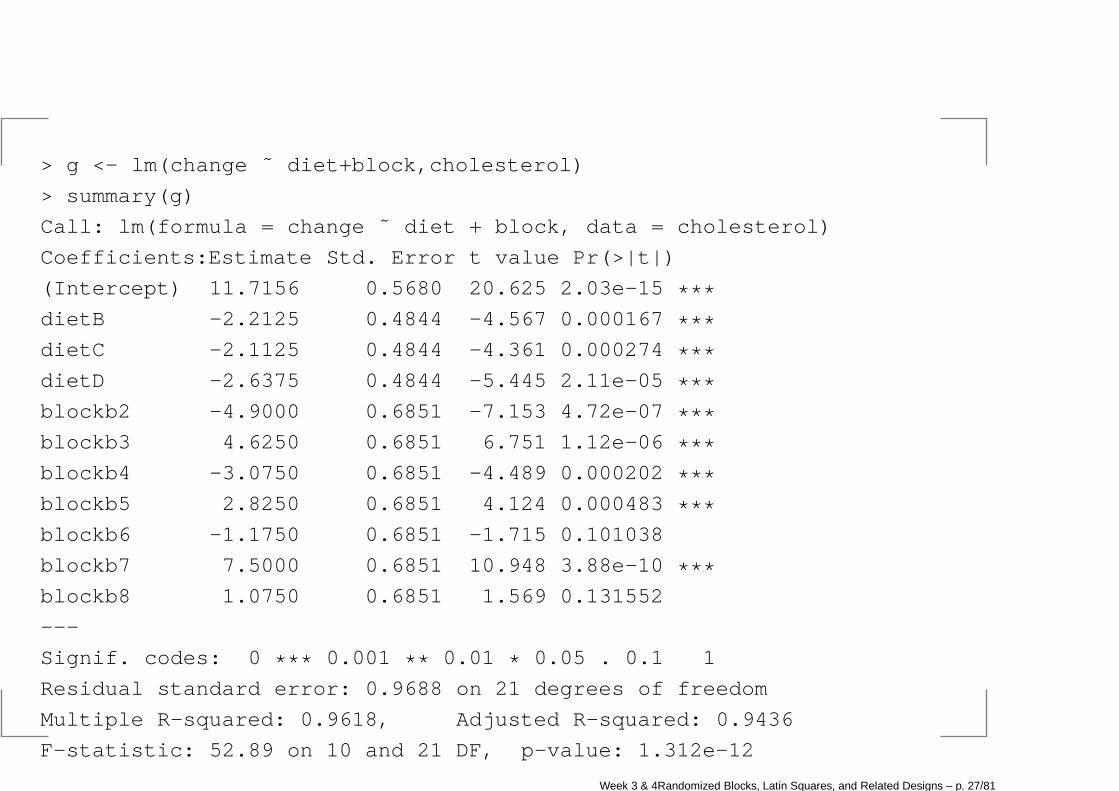
> g <- lm(change ˜ diet+block,cholesterol)
> summary(g)
Call: lm(formula = change ˜ diet + block, data = cholesterol)
Coefficients:Estimate Std. Error t value Pr(>|t|)
(Intercept) 11.7156 0.5680 20.625 2.03e-15 ***dietB -2.2125 0.4844 -4.567 0.000167 ***dietC -2.1125 0.4844 -4.361 0.000274 ***dietD -2.6375 0.4844 -5.445 2.11e-05 ***blockb2 -4.9000 0.6851 -7.153 4.72e-07 ***blockb3 4.6250 0.6851 6.751 1.12e-06 ***blockb4 -3.0750 0.6851 -4.489 0.000202 ***blockb5 2.8250 0.6851 4.124 0.000483 ***blockb6 -1.1750 0.6851 -1.715 0.101038
blockb7 7.5000 0.6851 10.948 3.88e-10 ***blockb8 1.0750 0.6851 1.569 0.131552
---
Signif. codes: 0 *** 0.001 ** 0.01 * 0.05 . 0.1 1
Residual standard error: 0.9688 on 21 degrees of freedom
Multiple R-squared: 0.9618, Adjusted R-squared: 0.9436
F-statistic: 52.89 on 10 and 21 DF, p-value: 1.312e-12
Week 3 & 4Randomized Blocks, Latin Squares, and Related Designs – p. 27/81
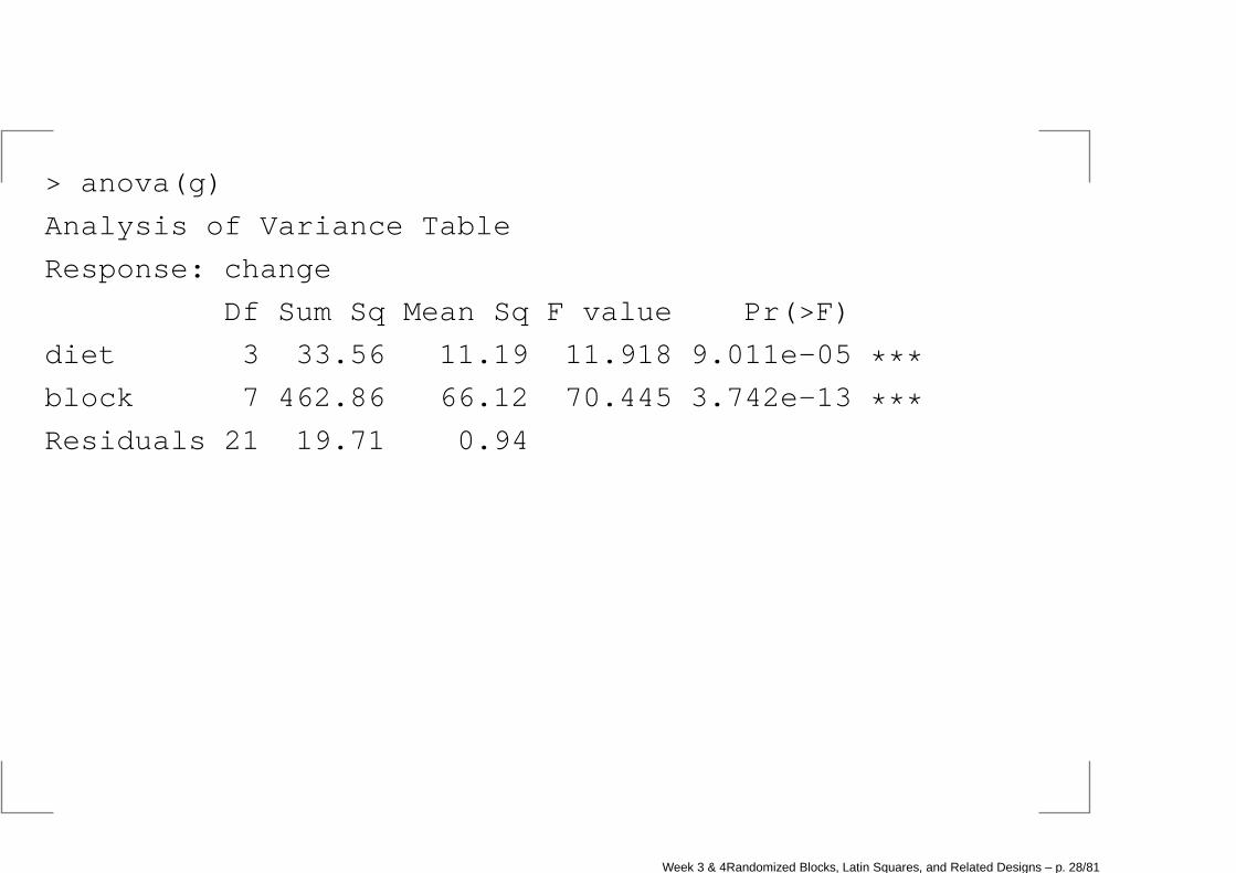
> anova(g)
Analysis of Variance Table
Response: change
Df Sum Sq Mean Sq F value Pr(>F)
diet 3 33.56 11.19 11.918 9.011e-05 ***block 7 462.86 66.12 70.445 3.742e-13 ***Residuals 21 19.71 0.94
Week 3 & 4Randomized Blocks, Latin Squares, and Related Designs – p. 28/81
3.2 Balanced Incomplete Block Design
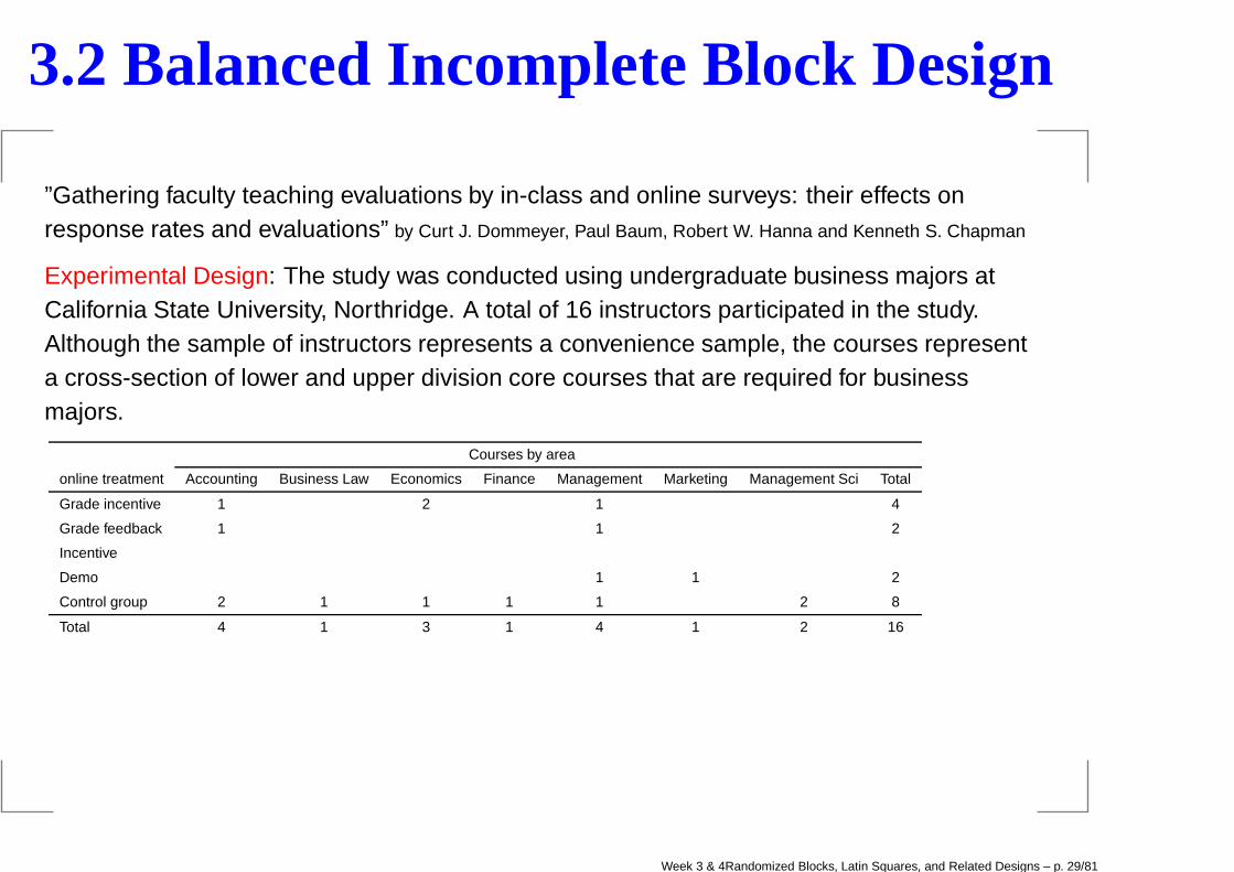
”Gathering faculty teaching evaluations by in-class and online surveys: their effects onresponse rates and evaluations” by Curt J. Dommeyer, Paul Baum, Robert W. Hanna and Kenneth S. Chapman
Experimental Design: The study was conducted using undergraduate business majors atCalifornia State University, Northridge. A total of 16 instructors participated in the study.Although the sample of instructors represents a convenience sample, the courses representa cross-section of lower and upper division core courses that are required for businessmajors.
Courses by area
online treatment Accounting Business Law Economics Finance Management Marketing Management Sci Total
Grade incentive 1 2 1 4
Grade feedback 1 1 2
Incentive
Demo 1 1 2
Control group 2 1 1 1 1 2 8
Total 4 1 3 1 4 1 2 16
Week 3 & 4Randomized Blocks, Latin Squares, and Related Designs – p. 29/81

Each of the instructors in this study was assigned to have one of his/her sectionsevaluated in-class and the other evaluated online. In the online evaluation, each
instructor was assigned either to a control group or to one of the following onlinetreatments:
1. a very modest grade incentive (one-quarter of a percent) for completing theonline evaluations;
2. an in-class demonstration of how to log on to the web site and complete theform;
3. an early grade feedback incentive in which students were told they wouldreceive early feedback of their course grades (by postcard and/or posting the
grades online) if at least two-thirds of the class completed online evaluations.
Week 3 & 4Randomized Blocks, Latin Squares, and Related Designs – p. 30/81
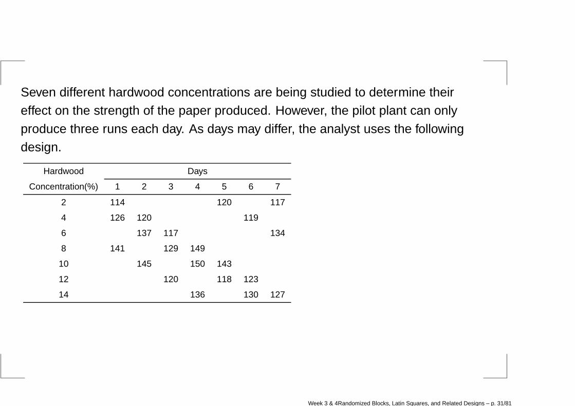
Seven different hardwood concentrations are being studied to determine theireffect on the strength of the paper produced. However, the pilot plant can only
produce three runs each day. As days may differ, the analyst uses the followingdesign.
Hardwood Days
Concentration(%) 1 2 3 4 5 6 7
2 114 120 117
4 126 120 119
6 137 117 134
8 141 129 149
10 145 150 143
12 120 118 123
14 136 130 127
Week 3 & 4Randomized Blocks, Latin Squares, and Related Designs – p. 31/81
Definition and notation
A Balanced Incomplete Block Design BIBD(N ,a,k,b,r,λ) isan incomplete block design in which
Week 3 & 4Randomized Blocks, Latin Squares, and Related Designs – p. 32/81
a: the number of treatments
k: the block size
b: the number of blocks
r: the number of times each treatment occurs
λ: the number of times each pair of treatments appearsin the same block
N : the number of observations
Week 3 & 4Randomized Blocks, Latin Squares, and Related Designs – p. 33/81
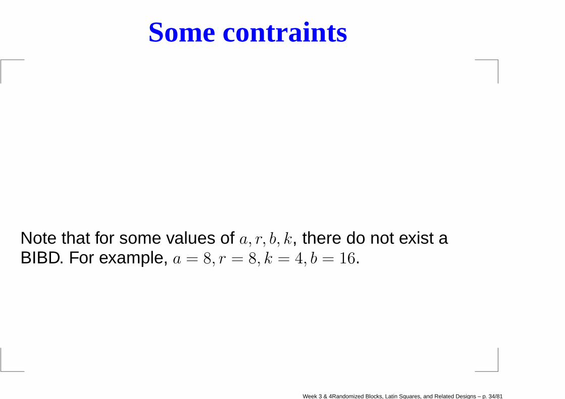
Some contraints
Note that for some values of a, r, b, k, there do not exist aBIBD. For example, a = 8, r = 8, k = 4, b = 16.
Week 3 & 4Randomized Blocks, Latin Squares, and Related Designs – p. 34/81
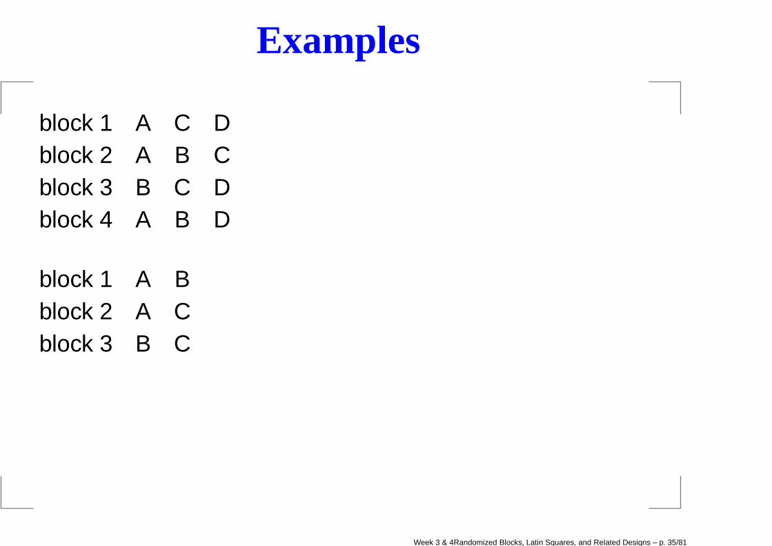
Examples
block 1 A C Dblock 2 A B Cblock 3 B C Dblock 4 A B D
block 1 A Bblock 2 A Cblock 3 B C
Week 3 & 4Randomized Blocks, Latin Squares, and Related Designs – p. 35/81
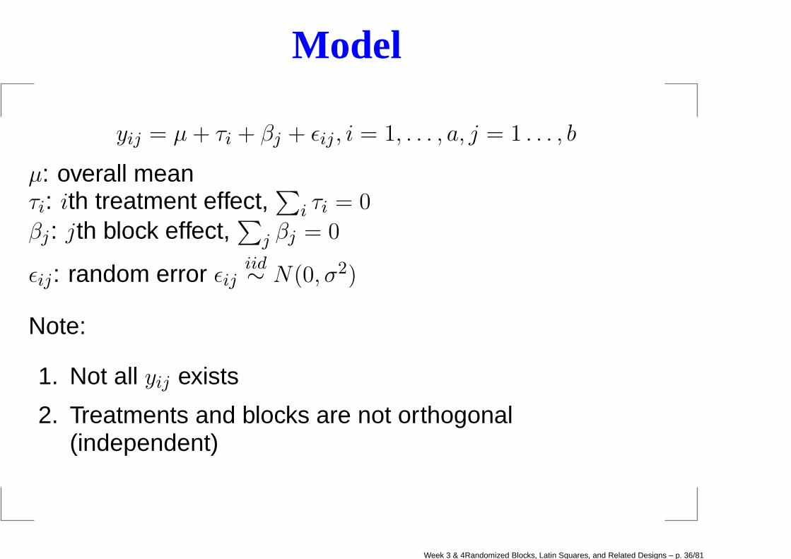
Model
yij = µ+ τi + βj + ǫij , i = 1, . . . , a, j = 1 . . . , b
µ: overall meanτi: ith treatment effect,
∑
i τi = 0
βj: jth block effect,∑
j βj = 0
ǫij: random error ǫijiid∼ N(0, σ2)
Note:
1. Not all yij exists
2. Treatments and blocks are not orthogonal(independent)
Week 3 & 4Randomized Blocks, Latin Squares, and Related Designs – p. 36/81
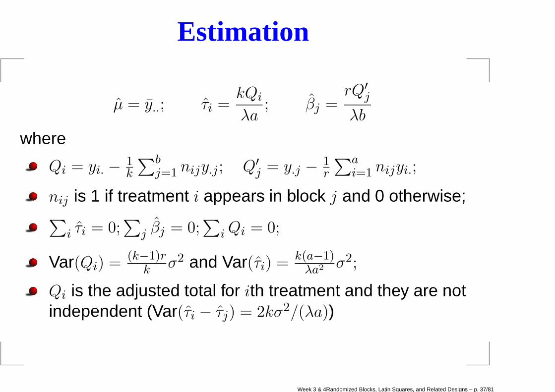
Estimation
µ = y..; τi =kQi
λa; βj =
rQ′
j
λb
where
Qi = yi. − 1k
∑bj=1 nijy.j ; Q′
j = y.j − 1r
∑ai=1 nijyi.;
nij is 1 if treatment i appears in block j and 0 otherwise;∑
i τi = 0;∑
j βj = 0;∑
iQi = 0;
Var(Qi) =(k−1)r
k σ2 and Var(τi) =k(a−1)λa2 σ2;
Qi is the adjusted total for ith treatment and they are notindependent (Var(τi − τj) = 2kσ2/(λa))
Week 3 & 4Randomized Blocks, Latin Squares, and Related Designs – p. 37/81

Note the blocks are incomplete and thus yi. − y.. is not an unbiasedestimate of τi.For exampleE(y1.) = µ+ τ1 + (β1 + β2 + β3)/3
E(y..) = µ
E(y1. − y..) = τ1 + (β1 + β2 + β3)/3
Week 3 & 4Randomized Blocks, Latin Squares, and Related Designs – p. 38/81

ANOVA Table
Define:
SSTotal =∑
i,j
(yij − y..)2 =
∑
i,j
y2ij −
y2..
N
SSBlocks = k∑
j
(y.j − y..)2 =
1
k
∑
j
y2.j −
y2..
N
SSTreatments(adjusted) =k∑a
i=1 Q2i
λa
SSError = SSTotal − SSBlocks − SSTreatments(adjusted)
Week 3 & 4Randomized Blocks, Latin Squares, and Related Designs – p. 39/81
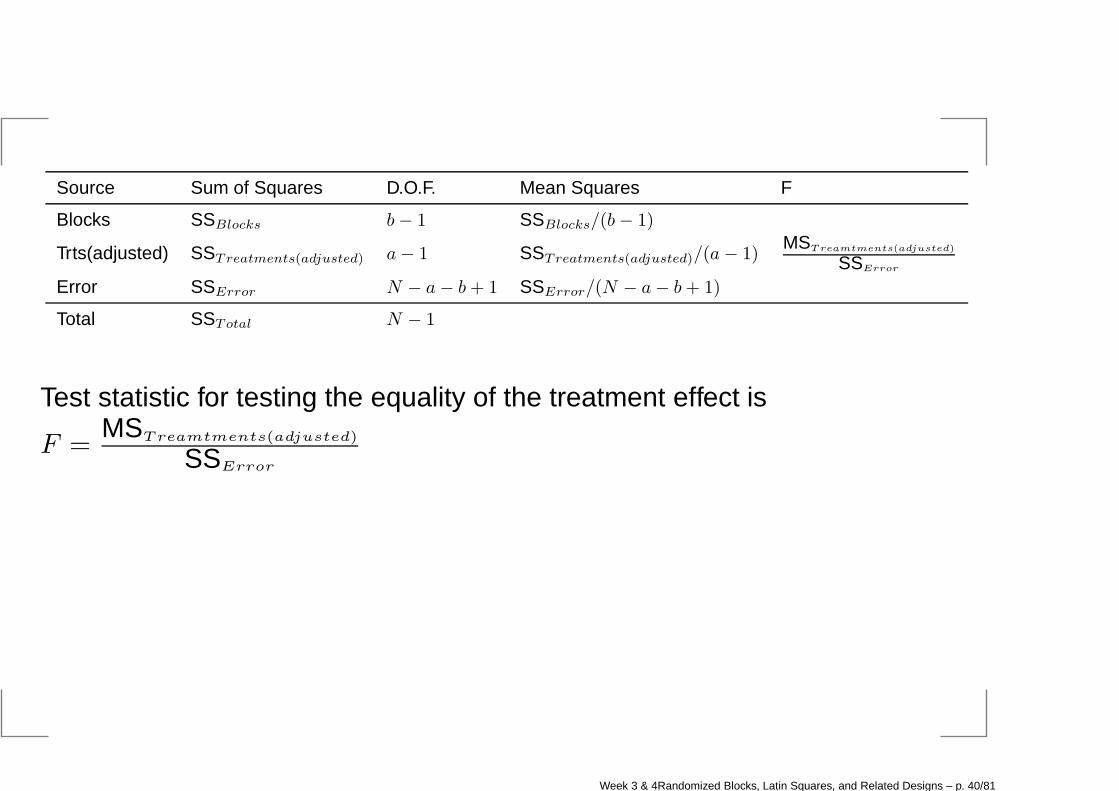
Source Sum of Squares D.O.F. Mean Squares F
Blocks SSBlocks b− 1 SSBlocks/(b− 1)
Trts(adjusted) SSTreatments(adjusted) a− 1 SSTreatments(adjusted)/(a− 1)MSTreamtments(adjusted)
SSError
Error SSError N − a− b+ 1 SSError/(N − a− b+ 1)
Total SSTotal N − 1
Test statistic for testing the equality of the treatment effect is
F =MSTreamtments(adjusted)
SSError
Week 3 & 4Randomized Blocks, Latin Squares, and Related Designs – p. 40/81
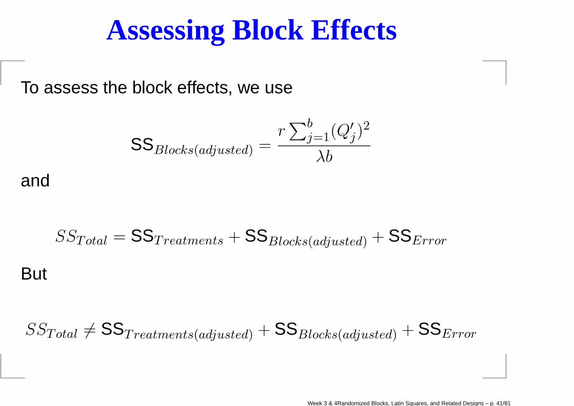
Assessing Block Effects
To assess the block effects, we use
SSBlocks(adjusted) =r∑b
j=1(Q′
j)2
λb
and
SSTotal = SSTreatments + SSBlocks(adjusted) + SSError
But
SSTotal 6= SSTreatments(adjusted) + SSBlocks(adjusted) + SSError
Week 3 & 4Randomized Blocks, Latin Squares, and Related Designs – p. 41/81

Confidence interval
For τi − τj
Fisher LSD CI
τi − τj ± tα/2,N−a−b+1
√
2k
λaMSError
Tukey’s CI
τi − τj ±qα,a,N−a−b+1√
2
√
2k
λaMSError
Week 3 & 4Randomized Blocks, Latin Squares, and Related Designs – p. 42/81
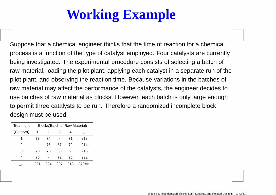
Working Example
Suppose that a chemical engineer thinks that the time of reaction for a chemicalprocess is a function of the type of catalyst employed. Four catalysts are currently
being investigated. The experimental procedure consists of selecting a batch ofraw material, loading the pilot plant, applying each catalyst in a separate run of the
pilot plant, and observing the reaction time. Because variations in the batches ofraw material may affect the performance of the catalysts, the engineer decides to
use batches of raw material as blocks. However, each batch is only large enoughto permit three catalysts to be run. Therefore a randomized incomplete block
design must be used.
Treatment Blocks(Batch of Raw Material)
(Catalyst) 1 2 3 4 yi.
1 73 74 - 71 218
2 - 75 67 72 214
3 73 75 68 - 216
4 75 - 72 75 222
y.j 221 224 207 218 870=y..
Week 3 & 4Randomized Blocks, Latin Squares, and Related Designs – p. 43/81
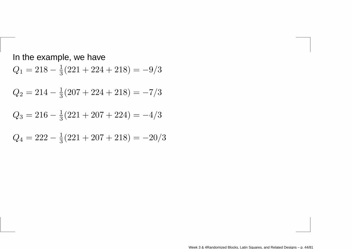
In the example, we haveQ1 = 218− 1
3 (221 + 224 + 218) = −9/3
Q2 = 214− 13 (207 + 224 + 218) = −7/3
Q3 = 216− 13 (221 + 207 + 224) = −4/3
Q4 = 222− 13 (221 + 207 + 218) = −20/3
Week 3 & 4Randomized Blocks, Latin Squares, and Related Designs – p. 44/81
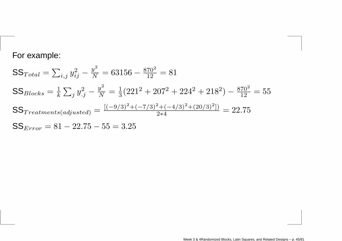
For example:
SSTotal =∑
i,j y2ij −
y2..
N = 63156− 8702
12 = 81
SSBlocks =1k
∑
j y2.j −
y2..
N = 13 (221
2 + 2072 + 2242 + 2182)− 8702
12 = 55
SSTreatments(adjusted) =[(−9/3)2+(−7/3)2+(−4/3)2+(20/3)2])
2∗4 = 22.75
SSError = 81− 22.75− 55 = 3.25
Week 3 & 4Randomized Blocks, Latin Squares, and Related Designs – p. 45/81
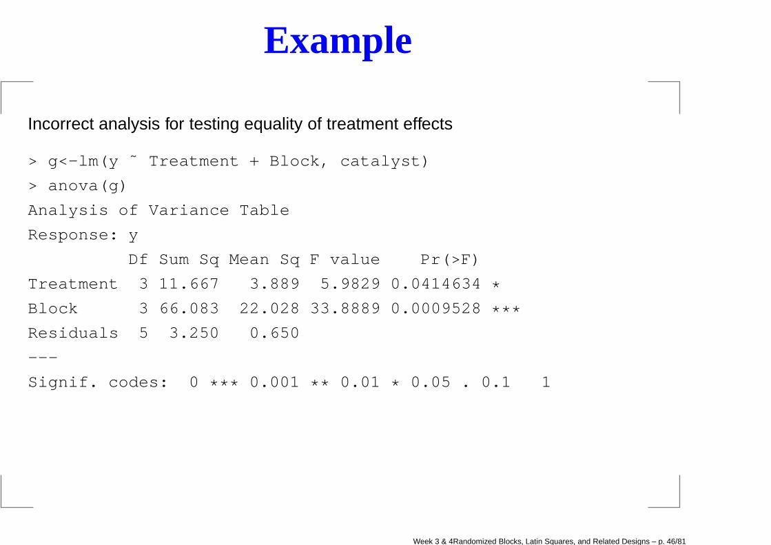
Example
Incorrect analysis for testing equality of treatment effects
> g<-lm(y ˜ Treatment + Block, catalyst)
> anova(g)
Analysis of Variance Table
Response: y
Df Sum Sq Mean Sq F value Pr(>F)
Treatment 3 11.667 3.889 5.9829 0.0414634 *Block 3 66.083 22.028 33.8889 0.0009528 ***Residuals 5 3.250 0.650
---
Signif. codes: 0 *** 0.001 ** 0.01 * 0.05 . 0.1 1
Week 3 & 4Randomized Blocks, Latin Squares, and Related Designs – p. 46/81
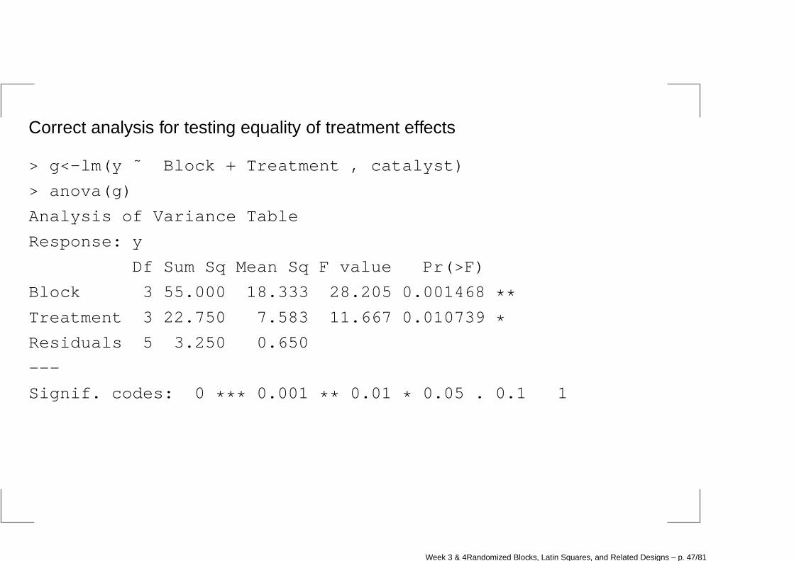
Correct analysis for testing equality of treatment effects
> g<-lm(y ˜ Block + Treatment , catalyst)
> anova(g)
Analysis of Variance Table
Response: y
Df Sum Sq Mean Sq F value Pr(>F)
Block 3 55.000 18.333 28.205 0.001468 **Treatment 3 22.750 7.583 11.667 0.010739 *Residuals 5 3.250 0.650
---
Signif. codes: 0 *** 0.001 ** 0.01 * 0.05 . 0.1 1
Week 3 & 4Randomized Blocks, Latin Squares, and Related Designs – p. 47/81

#set the parameters
a<-4 b<-4 k<-3 r<-3 n<-12
lambda<-r * (k-1)/(a-1)
# create n_ij
Nij<-matrix(0,a,a)
for(i in 1:n) Nij[as.integer(Treatment[i]),as.integer( Block[i])]<-1
# compute y_i.
ysumi<-vector(’numeric’,a)
for(i in 1:a) ysumi[i]<-sum(y[((i-1) * r+1):(i * r)])
#compute y_.j
ysumj<-vector(’numeric’,b)
for(i in 1:n) {ysumj[as.integer(Block[i])]<- ysumj[as.i nteger(Block[i])] + y[i]}
#compute Q_i
Qi<-vector("numeric",a)
for(i in 1:a) Qi[i]<-ysumi[i]-sum(Nij[i,] * ysumj)/k
#compute hat of tau_i
tauihat<-k * Qi/(lambda * a)
Week 3 & 4Randomized Blocks, Latin Squares, and Related Designs – p. 48/81
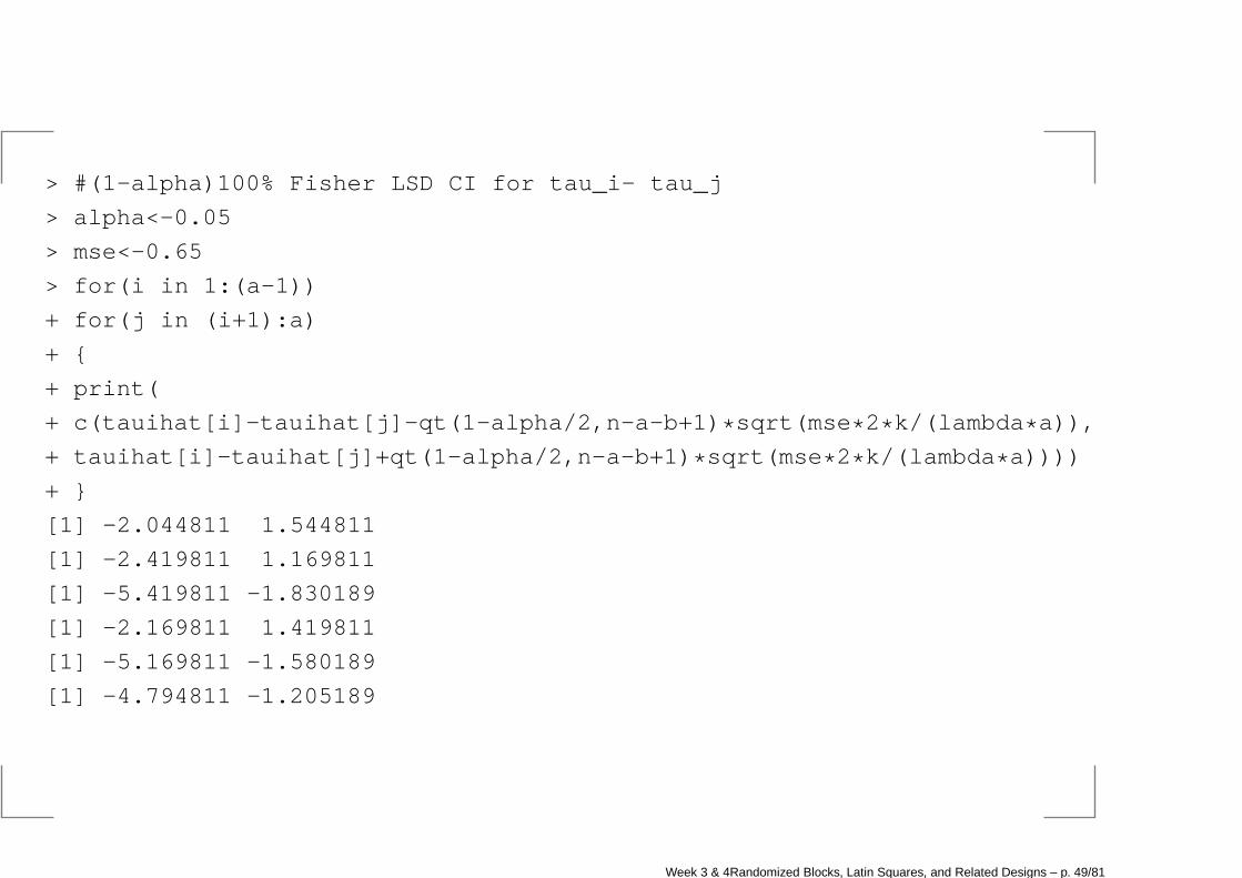
> #(1-alpha)100% Fisher LSD CI for tau_i- tau_j
> alpha<-0.05
> mse<-0.65
> for(i in 1:(a-1))
+ for(j in (i+1):a)
+ {
+ print(
+ c(tauihat[i]-tauihat[j]-qt(1-alpha/2,n-a-b+1) * sqrt(mse * 2* k/(lambda * a)),
+ tauihat[i]-tauihat[j]+qt(1-alpha/2,n-a-b+1) * sqrt(mse * 2* k/(lambda * a))))
+ }
[1] -2.044811 1.544811
[1] -2.419811 1.169811
[1] -5.419811 -1.830189
[1] -2.169811 1.419811
[1] -5.169811 -1.580189
[1] -4.794811 -1.205189
Week 3 & 4Randomized Blocks, Latin Squares, and Related Designs – p. 49/81
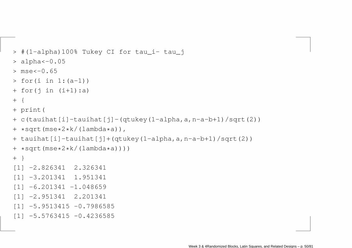
> #(1-alpha)100% Tukey CI for tau_i- tau_j
> alpha<-0.05
> mse<-0.65
> for(i in 1:(a-1))
+ for(j in (i+1):a)
+ {
+ print(
+ c(tauihat[i]-tauihat[j]-(qtukey(1-alpha,a,n-a-b+1) /sqrt(2))
+ * sqrt(mse * 2* k/(lambda * a)),
+ tauihat[i]-tauihat[j]+(qtukey(1-alpha,a,n-a-b+1)/s qrt(2))
+ * sqrt(mse * 2* k/(lambda * a))))
+ }
[1] -2.826341 2.326341
[1] -3.201341 1.951341
[1] -6.201341 -1.048659
[1] -2.951341 2.201341
[1] -5.9513415 -0.7986585
[1] -5.5763415 -0.4236585
Week 3 & 4Randomized Blocks, Latin Squares, and Related Designs – p. 50/81
Other incomplete block designs
Youden square
Partially balanced incomplete block design
Cubic and rectangular Lattices
Cyclic designs
Week 3 & 4Randomized Blocks, Latin Squares, and Related Designs – p. 51/81
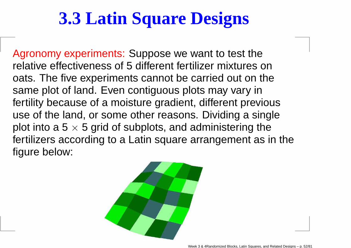
3.3 Latin Square Designs
Agronomy experiments: Suppose we want to test therelative effectiveness of 5 different fertilizer mixtures onoats. The five experiments cannot be carried out on thesame plot of land. Even contiguous plots may vary infertility because of a moisture gradient, different previoususe of the land, or some other reasons. Dividing a singleplot into a 5 × 5 grid of subplots, and administering thefertilizers according to a Latin square arrangement as in thefigure below:
Week 3 & 4Randomized Blocks, Latin Squares, and Related Designs – p. 52/81

Typewriters experiments: A company is interested inpurchasing one brand of typewriter from among the 5 kindsavailable in the market. To make decision, a study isperformed to evaluate the typewriter. It is suspected thatthe time of the day as well the day of the week in which thetest is carried out affects the output on the machine.
DaysShifts
1 2 3 4 5 Total TreatmentsMon. 10 15 11 13 9 58 D B A C ETue. 10 12 16 10 12 60 E C B D AWed. 19 8 12 10 8 57 B E C A DThu. 9 12 10 14 12 57 A D E B CFri. 12 11 8 10 15 56 C A D E BTotal 60 58 57 57 56 288
Week 3 & 4Randomized Blocks, Latin Squares, and Related Designs – p. 53/81

Example: A hardness testing machine presses a pointed rod (the ‘tip’) into a metalspecimen (a ‘coupon’), with a known force. The depth of the depression is a
measure of the hardness of the specimen. It is feared that, depending on the kindof tip used, the machine might give different readings. The experimenter wants 4
observations on each of the 4 types of tips. Suppose that the ‘coupon’ and the‘operator’ of the testing machine are thought to be factors. Suppose there are
p = 4 operators, p = 4 coupons, and p = 4 tips. The first two are nuisance factors,the last is the treatment factor.
Operator
Coupon k = 1 k = 2 k = 3 k = 4
i = 1 A = 9.3 B = 9.3 C = 9.5 D = 10.2
i = 2 B = 9.4 A = 9.4 D = 10 C = 9.7
i = 3 C = 9.2 D = 9.6 A = 9.6 B = 9.9
i = 4 D = 9.7 C = 9.4 B = 9.8 A = 10
Week 3 & 4Randomized Blocks, Latin Squares, and Related Designs – p. 54/81
Definition
Consider one treatment factor and two nuisance/blockingfactors. A design is called Latin square design if eachtreatment appears exactly once in each row and in eachcolumn.
The number of levels of each blocking factor must equalthe number of levels of the treatment factor.
Small run sizes
RandomizationRandomly select a Latin square.Randomize the experiment units and trial orders.
Week 3 & 4Randomized Blocks, Latin Squares, and Related Designs – p. 55/81
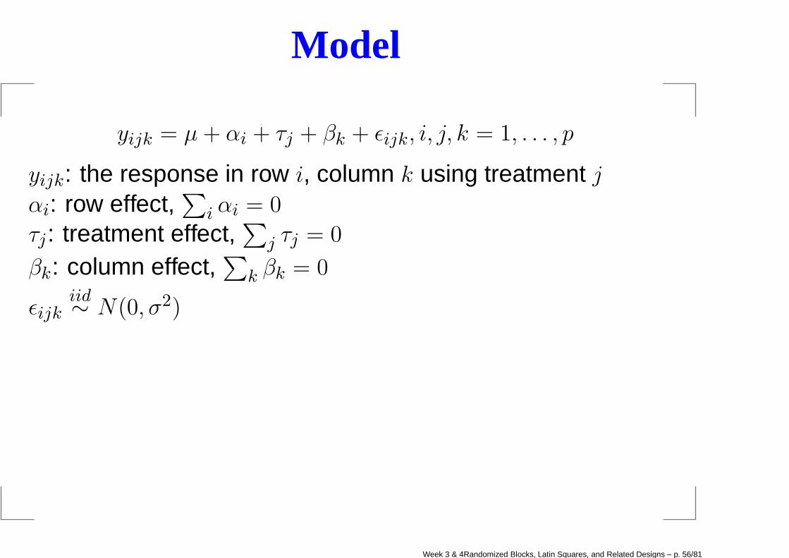
Model
yijk = µ+ αi + τj + βk + ǫijk, i, j, k = 1, . . . , p
yijk: the response in row i, column k using treatment jαi: row effect,
∑
i αi = 0
τj: treatment effect,∑
j τj = 0
βk: column effect,∑
k βk = 0
ǫijkiid∼ N(0, σ2)
Week 3 & 4Randomized Blocks, Latin Squares, and Related Designs – p. 56/81
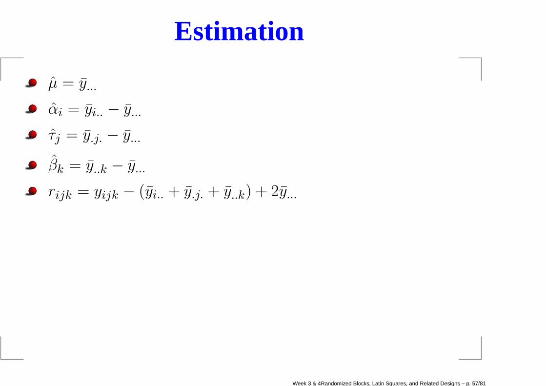
Estimation
µ = y...
αi = yi.. − y...
τj = y.j. − y...
βk = y..k − y...
rijk = yijk − (yi.. + y.j. + y..k) + 2y...
Week 3 & 4Randomized Blocks, Latin Squares, and Related Designs – p. 57/81
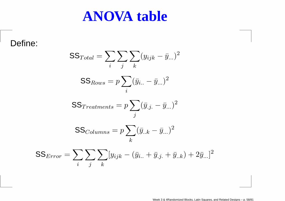
ANOVA table
Define:SSTotal =
∑
i
∑
j
∑
k
(yijk − y...)2
SSRows = p∑
i
(yi.. − y...)2
SSTreatments = p∑
j
(y.j. − y...)2
SSColumns = p∑
k
(y..k − y...)2
SSError =∑
i
∑
j
∑
k
[yijk − (yi.. + y.j. + y..k) + 2y...]2
Week 3 & 4Randomized Blocks, Latin Squares, and Related Designs – p. 58/81
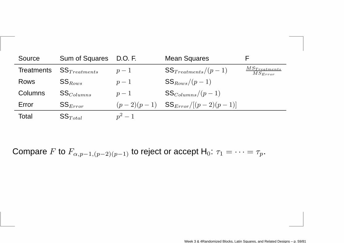
Source Sum of Squares D.O. F. Mean Squares F
Treatments SSTreatments p− 1 SSTreatments/(p− 1) MSTreatments
MSError
Rows SSRows p− 1 SSRows/(p− 1)
Columns SSColumns p− 1 SSColumns/(p− 1)
Error SSError (p− 2)(p− 1) SSError/[(p− 2)(p− 1)]
Total SSTotal p2 − 1
Compare F to Fα,p−1,(p−2)(p−1) to reject or accept H0: τ1 = · · · = τp.
Week 3 & 4Randomized Blocks, Latin Squares, and Related Designs – p. 59/81
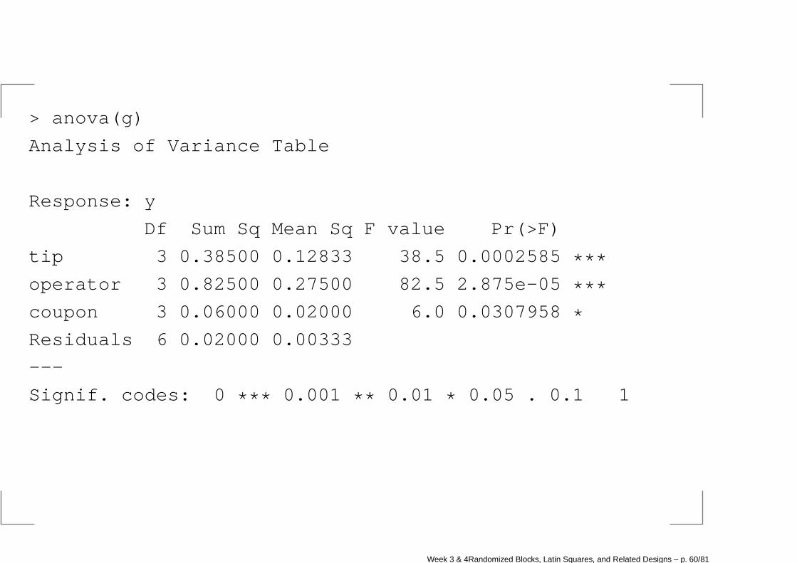
> anova(g)
Analysis of Variance Table
Response: y
Df Sum Sq Mean Sq F value Pr(>F)
tip 3 0.38500 0.12833 38.5 0.0002585 ***operator 3 0.82500 0.27500 82.5 2.875e-05 ***coupon 3 0.06000 0.02000 6.0 0.0307958 *Residuals 6 0.02000 0.00333
---
Signif. codes: 0 *** 0.001 ** 0.01 * 0.05 . 0.1 1
Week 3 & 4Randomized Blocks, Latin Squares, and Related Designs – p. 60/81
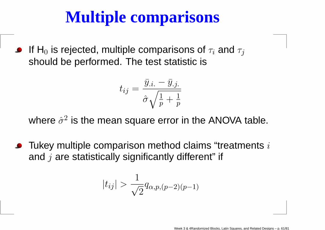
Multiple comparisons
If H0 is rejected, multiple comparisons of τi and τjshould be performed. The test statistic is
tij =y.i. − y.j.
σ√
1p +
1p
where σ2 is the mean square error in the ANOVA table.
Tukey multiple comparison method claims “treatments iand j are statistically significantly different” if
|tij| >1√2qα,p,(p−2)(p−1)
Week 3 & 4Randomized Blocks, Latin Squares, and Related Designs – p. 61/81

Application
Crossover design is a type of randomized clinical trial. Each participants in thedesign is randomized to either group 1 or group 2. All participants in group 1
receive drug A in the first treatment period and drug B in the second period. Allparticipants in group 2 receive drug B in the first treatment period and drug A in the
second treatment period. Often there is a washout period between the two activedrug periods. During the washout period, they receive no study medication. The
purpose of the washout period is to reduce the likelihood that study medicationtaken in the first period will have an effect that carries over the next period.
Latin Squares
I II III IV V
Subject 1 2 3 4 5 6 7 8 9 10
Period 1 A B B A B A A B A B
Period 2 B A A B A B B A B A
Week 3 & 4Randomized Blocks, Latin Squares, and Related Designs – p. 62/81
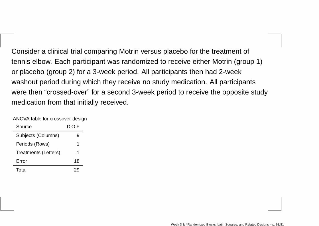
Consider a clinical trial comparing Motrin versus placebo for the treatment oftennis elbow. Each participant was randomized to receive either Motrin (group 1)
or placebo (group 2) for a 3-week period. All participants then had 2-weekwashout period during which they receive no study medication. All participants
were then “crossed-over” for a second 3-week period to receive the opposite studymedication from that initially received.
ANOVA table for crossover design
Source D.O.F
Subjects (Columns) 9
Periods (Rows) 1
Treatments (Letters) 1
Error 18
Total 29
Week 3 & 4Randomized Blocks, Latin Squares, and Related Designs – p. 63/81

3.3 Graeco-Latin Squares
Definition: Orthogonal Latin squaresTwo Latin squares are said to be orthogonal if each pair ofletters appears exactly once in the superimposed squares.The superimposed square is called Graeco-Latin square.
Aα Bβ Cγ
Bγ Cα Aβ
Cβ Aγ Bα
Week 3 & 4Randomized Blocks, Latin Squares, and Related Designs – p. 64/81

Model
yijkl = µ+ θi + τj + ωk + φl + ǫijkl, i, j, k, l = 1, . . . , p
yijkl: the observation in row i and column l for Latin letter jand Greek letter k.θi: ith row effectτj: jth Latin letter treatment effectωk: kth Greek letter treatment effectφl: lth column effect
ǫijkliid∼ N(0, σ2)
Week 3 & 4Randomized Blocks, Latin Squares, and Related Designs – p. 65/81

ANOVA Table
Source Sum of Squares D.O.F
Rows p∑
i(yi... − y....)2 p− 1
Latin letter treatments p∑
j(y.j.. − y....)2 p− 1
Greek letter treatments p∑
k(y..k. − y....)2 p− 1
Columns p∑
l(y...l − y....)2 p− 1
Error SSError(by substraction) (p− 3)(p− 1)
Total∑
i
∑
j
∑
k
∑
l(yijkl − y....)2 p2 − 1
F-test and Tukey’s multiple comparison are similar as those in Latinsquare design.
Week 3 & 4Randomized Blocks, Latin Squares, and Related Designs – p. 66/81

3.5 Analysis of Covariance (ANCOVA)
Consider an experiment (Flurry, 1939) to study the breaking strength (y) ingrams of three types of starch film. The breaking strength is also known todepend on the thickness of the film (x) as measured in 10−4 inches.Because film thickness varies from run to run and its values cannot becontrolled or chosen prior to the experiment, it should be treated as acovariate whose effect on strength needs to be accounted for beforecomparing the three types of starch.
Objective: perform the treatment comparisons by incorporating theinformation of auxiliary covariate x
Week 3 & 4Randomized Blocks, Latin Squares, and Related Designs – p. 67/81
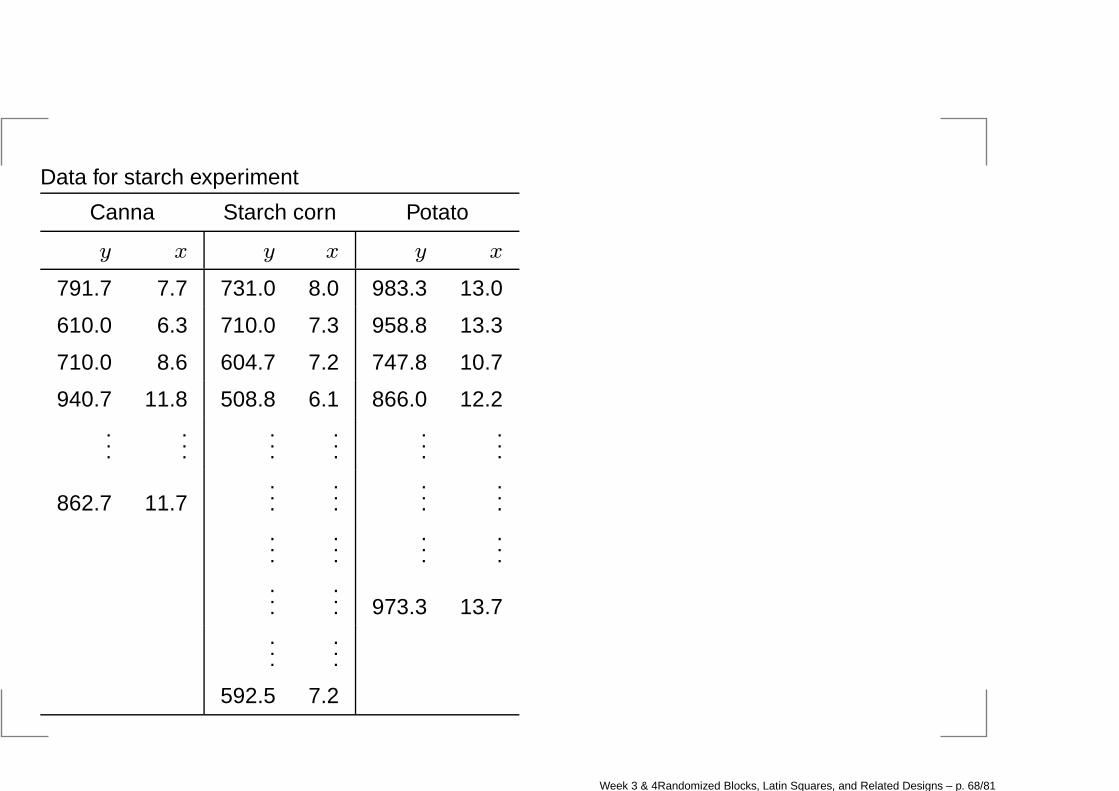
Data for starch experiment
Canna Starch corn Potato
y x y x y x
791.7 7.7 731.0 8.0 983.3 13.0
610.0 6.3 710.0 7.3 958.8 13.3
710.0 8.6 604.7 7.2 747.8 10.7
940.7 11.8 508.8 6.1 866.0 12.2...
......
......
...
862.7 11.7...
......
......
......
......
... 973.3 13.7...
...
592.5 7.2
Week 3 & 4Randomized Blocks, Latin Squares, and Related Designs – p. 68/81
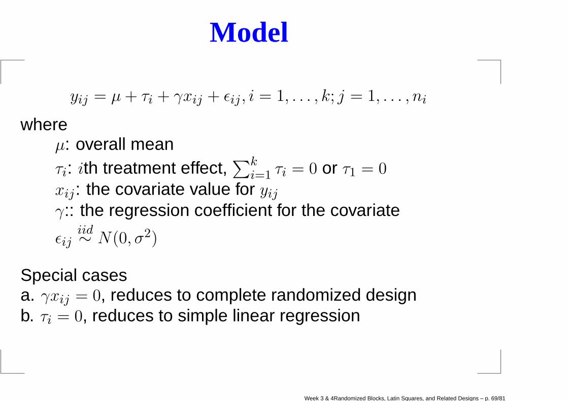
Model
yij = µ+ τi + γxij + ǫij , i = 1, . . . , k; j = 1, . . . , ni
whereµ: overall meanτi: ith treatment effect,
∑ki=1 τi = 0 or τ1 = 0
xij: the covariate value for yijγ:: the regression coefficient for the covariate
ǫijiid∼ N(0, σ2)
Special casesa. γxij = 0, reduces to complete randomized designb. τi = 0, reduces to simple linear regression
Week 3 & 4Randomized Blocks, Latin Squares, and Related Designs – p. 69/81

Estimation
Assume τ1 = 0We rewrite the model such that
y = Xβ + ǫ
where
y =
y11...
y1n1
...yk1...
yknk
, x =
1 0 0 0 0 x11
1...
......
......
1 0 0 0 0 x1n1
1 1 0 0 0 x21
1...
......
......
1 1 0 0 0 x2n2
......
......
......
1 0 0 0 1 xk1
1...
......
......
1 0 0 0 1 xknk
, β =
µ
τ2...τkγ
, ǫ =
ǫ11...
ǫ1n1
...ǫk1...
ǫknk
Week 3 & 4Randomized Blocks, Latin Squares, and Related Designs – p. 70/81
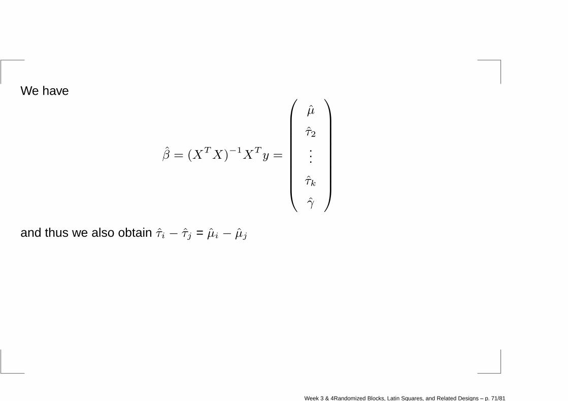
We have
β = (XTX)−1XT y =
µ
τ2...
τk
γ
and thus we also obtain τi − τj = µi − µj
Week 3 & 4Randomized Blocks, Latin Squares, and Related Designs – p. 71/81
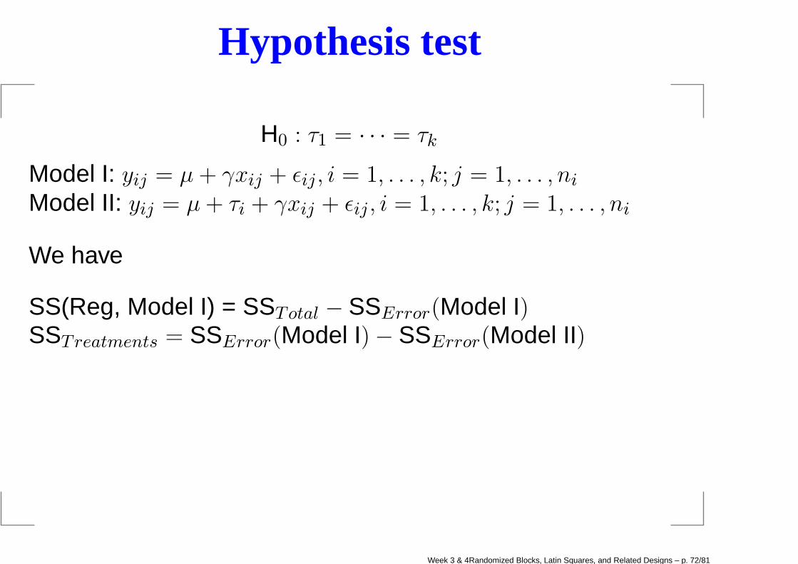
Hypothesis test
H0 : τ1 = · · · = τk
Model I: yij = µ+ γxij + ǫij, i = 1, . . . , k; j = 1, . . . , niModel II: yij = µ+ τi + γxij + ǫij , i = 1, . . . , k; j = 1, . . . , ni
We have
SS(Reg, Model I) = SSTotal − SSError(Model I)SSTreatments = SSError(Model I)− SSError(Model II)
Week 3 & 4Randomized Blocks, Latin Squares, and Related Designs – p. 72/81
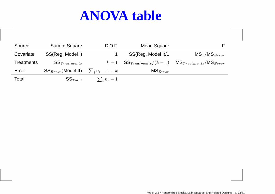
ANOVA table
Source Sum of Square D.O.F. Mean Square F
Covariate SS(Reg, Model I) 1 SS(Reg, Model I)/1 MSx/MSError
Treatments SSTreatments k − 1 SSTreatments/(k − 1) MSTreatments/MSError
Error SSError(Model II)∑
ini − 1− k MSError
Total SSTotal
∑
ini − 1
Week 3 & 4Randomized Blocks, Latin Squares, and Related Designs – p. 73/81

Multiple Comparisons
To compute Var(τi − τj), note that
Var(τi − τj) = Var(τi) + Var(τj)− 2Cov(τi, τj).
Use the fact Var(β) = σ2(XTX)−1 in multiple regression.
Test statistic tij =τi−τj
√
ˆVar(τi−τj)
Week 3 & 4Randomized Blocks, Latin Squares, and Related Designs – p. 74/81
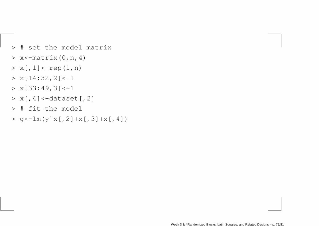
> # set the model matrix
> x<-matrix(0,n,4)
> x[,1]<-rep(1,n)
> x[14:32,2]<-1
> x[33:49,3]<-1
> x[,4]<-dataset[,2]
> # fit the model
> g<-lm(y˜x[,2]+x[,3]+x[,4])
Week 3 & 4Randomized Blocks, Latin Squares, and Related Designs – p. 75/81
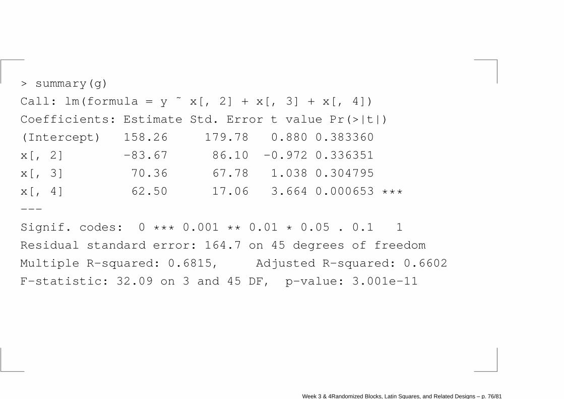
> summary(g)
Call: lm(formula = y ˜ x[, 2] + x[, 3] + x[, 4])
Coefficients: Estimate Std. Error t value Pr(>|t|)
(Intercept) 158.26 179.78 0.880 0.383360
x[, 2] -83.67 86.10 -0.972 0.336351
x[, 3] 70.36 67.78 1.038 0.304795
x[, 4] 62.50 17.06 3.664 0.000653 ***---
Signif. codes: 0 *** 0.001 ** 0.01 * 0.05 . 0.1 1
Residual standard error: 164.7 on 45 degrees of freedom
Multiple R-squared: 0.6815, Adjusted R-squared: 0.6602
F-statistic: 32.09 on 3 and 45 DF, p-value: 3.001e-11
Week 3 & 4Randomized Blocks, Latin Squares, and Related Designs – p. 76/81
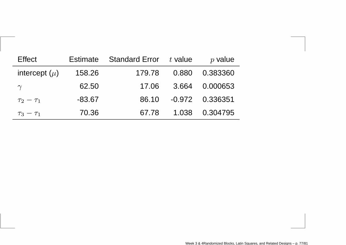
Effect Estimate Standard Error t value p value
intercept (µ) 158.26 179.78 0.880 0.383360
γ 62.50 17.06 3.664 0.000653
τ2 − τ1 -83.67 86.10 -0.972 0.336351
τ3 − τ1 70.36 67.78 1.038 0.304795
Week 3 & 4Randomized Blocks, Latin Squares, and Related Designs – p. 77/81
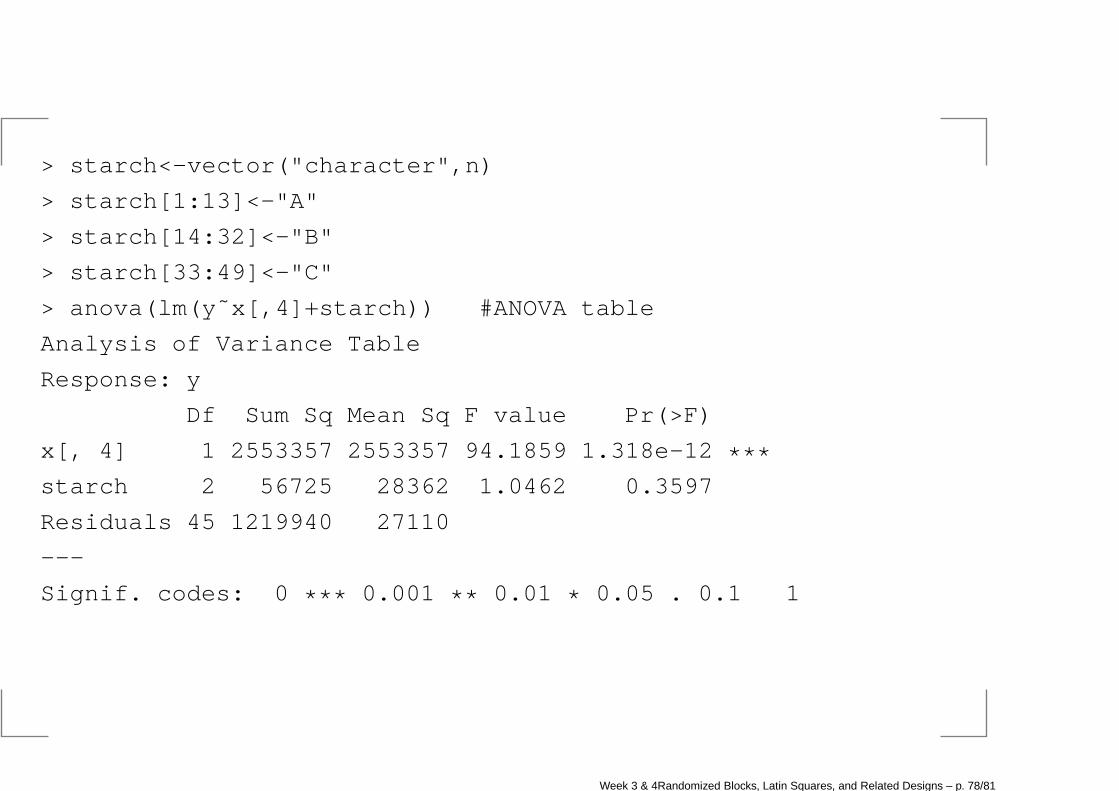
> starch<-vector("character",n)
> starch[1:13]<-"A"
> starch[14:32]<-"B"
> starch[33:49]<-"C"
> anova(lm(y˜x[,4]+starch)) #ANOVA table
Analysis of Variance Table
Response: y
Df Sum Sq Mean Sq F value Pr(>F)
x[, 4] 1 2553357 2553357 94.1859 1.318e-12 ***starch 2 56725 28362 1.0462 0.3597
Residuals 45 1219940 27110
---
Signif. codes: 0 *** 0.001 ** 0.01 * 0.05 . 0.1 1
Week 3 & 4Randomized Blocks, Latin Squares, and Related Designs – p. 78/81
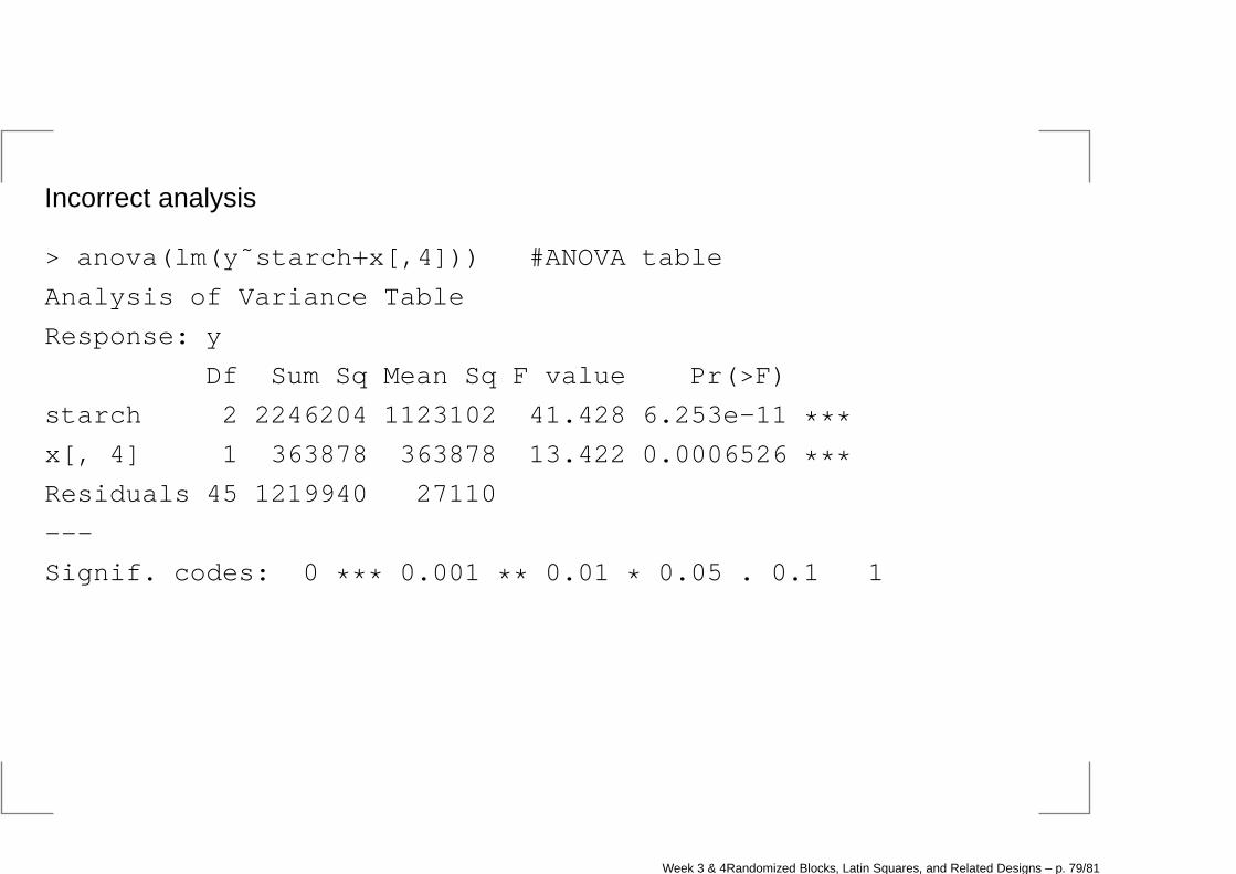
Incorrect analysis
> anova(lm(y˜starch+x[,4])) #ANOVA table
Analysis of Variance Table
Response: y
Df Sum Sq Mean Sq F value Pr(>F)
starch 2 2246204 1123102 41.428 6.253e-11 ***x[, 4] 1 363878 363878 13.422 0.0006526 ***Residuals 45 1219940 27110
---
Signif. codes: 0 *** 0.001 ** 0.01 * 0.05 . 0.1 1
Week 3 & 4Randomized Blocks, Latin Squares, and Related Designs – p. 79/81
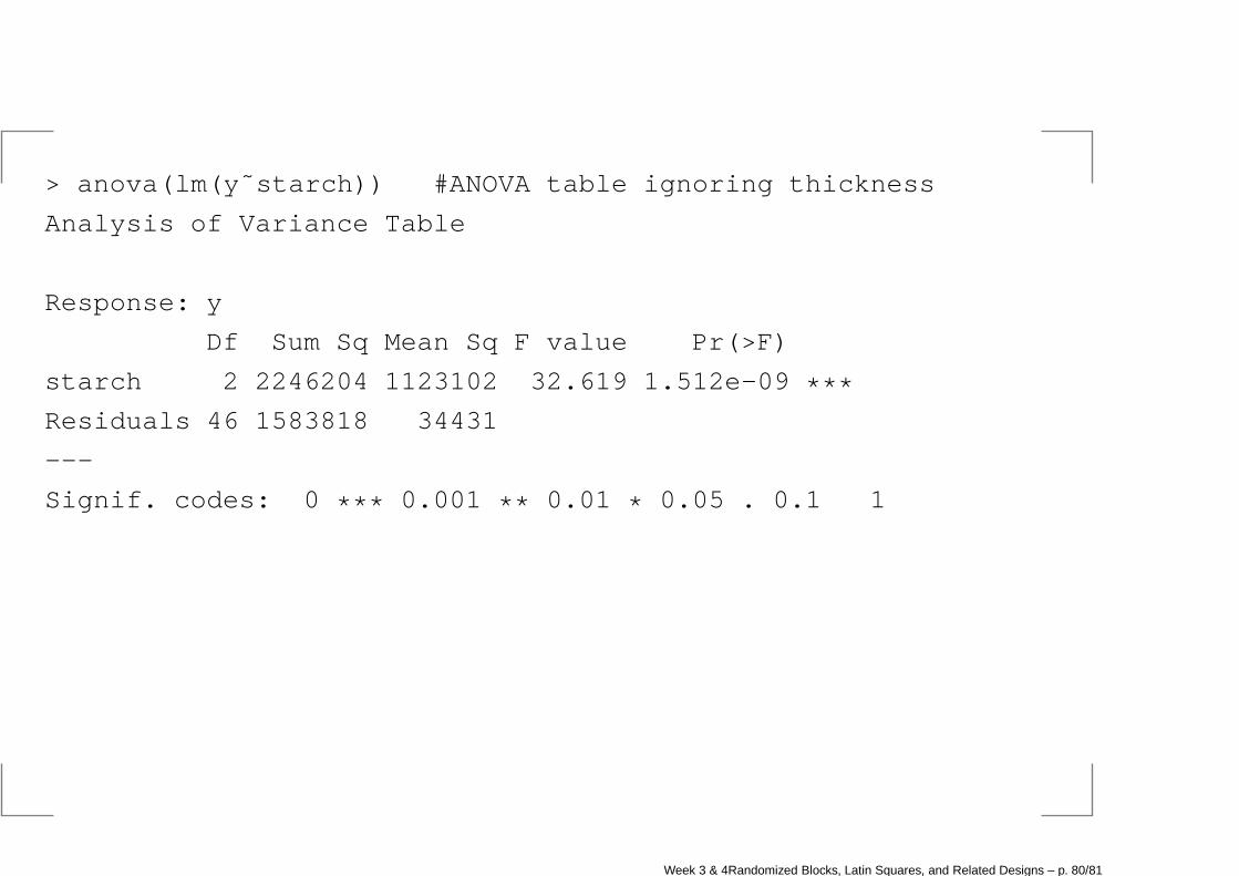
> anova(lm(y˜starch)) #ANOVA table ignoring thickness
Analysis of Variance Table
Response: y
Df Sum Sq Mean Sq F value Pr(>F)
starch 2 2246204 1123102 32.619 1.512e-09 ***Residuals 46 1583818 34431
---
Signif. codes: 0 *** 0.001 ** 0.01 * 0.05 . 0.1 1
Week 3 & 4Randomized Blocks, Latin Squares, and Related Designs – p. 80/81
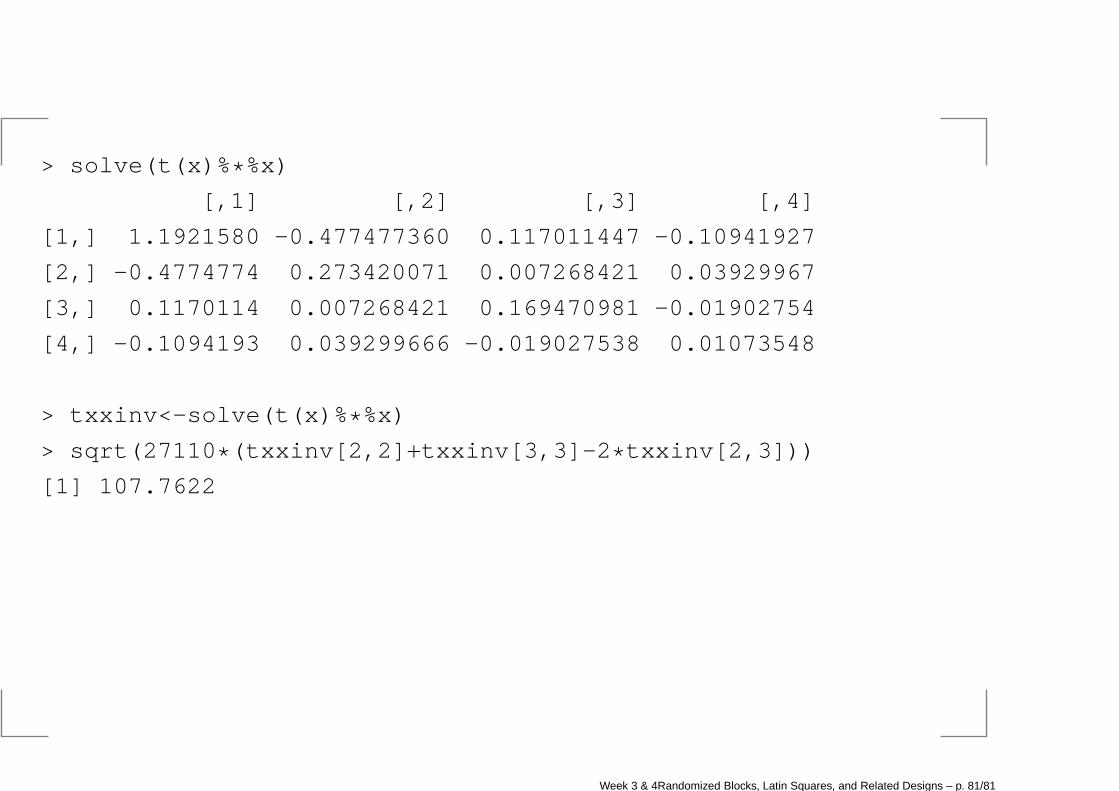
> solve(t(x)% * %x)
[,1] [,2] [,3] [,4]
[1,] 1.1921580 -0.477477360 0.117011447 -0.10941927
[2,] -0.4774774 0.273420071 0.007268421 0.03929967
[3,] 0.1170114 0.007268421 0.169470981 -0.01902754
[4,] -0.1094193 0.039299666 -0.019027538 0.01073548
> txxinv<-solve(t(x)% * %x)
> sqrt(27110 * (txxinv[2,2]+txxinv[3,3]-2 * txxinv[2,3]))
[1] 107.7622
Week 3 & 4Randomized Blocks, Latin Squares, and Related Designs – p. 81/81