Embed Size (px)
Citation preview
Surveying
Prof. Bharat Lohani
Department of Civil Engineering
Indian Institute of Technology, Kanpur
Module - 7
Lecture - 3
Levelling and Contouring
(Refer Slide Time: 00:21)
Welcome to this lecture series on basic surveying. And today, we will be talking about
again module 7, which is Levelling and Contouring, and today, we are in lecture number
3 of that.
(Refer Slide Time: 00:33)
What we have done so far? Particularly in our last lecture: we understood the terms back
sight and foresight; why do we balance them? Then, we also looked into the various
levelling instruments; we had the demonstrations with the instrument also. We looked
into some more things; for example, the sensitivity of the bubble tube, and as well as, if
at all there is some problem with the level - the meaning is, we see collimation error, non
parallelism error - how to adjust that physically working with the instrument, how to take
care of that; though, we know by balancing back sight and foresight we can eliminate the
resulting error. So, this is all what we have seen.
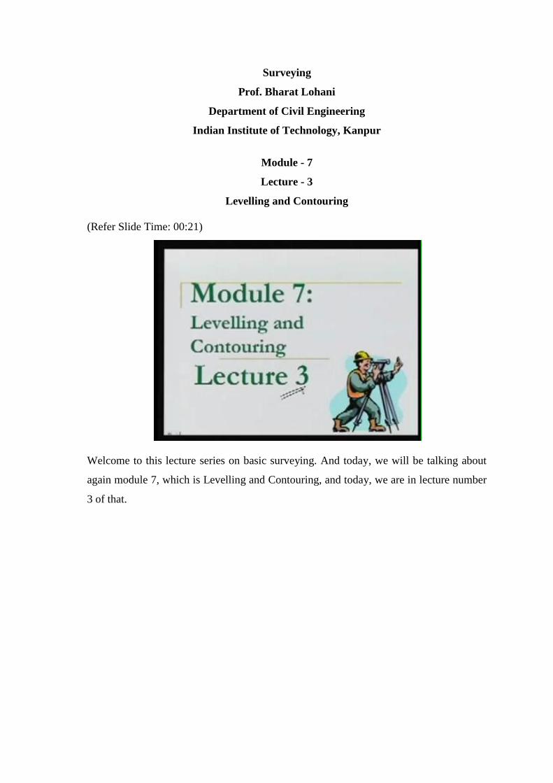
What will we do today? We will be looking into the actual levelling procedure, which
are height of the instrument, and rise and fall methods. Then, we will be looking into
some sources of error, and one important thing - that is acceptable misclosure error.
Finally, what are the types of the levelling? Reciprocal, profile, cross-sectioning, and
precise - these different kinds of things we will see today. So, we will start with our
levelling procedures. Levelling procedures means how actually we perform the levelling
there in the field.
(Refer Slide Time: 02:05)
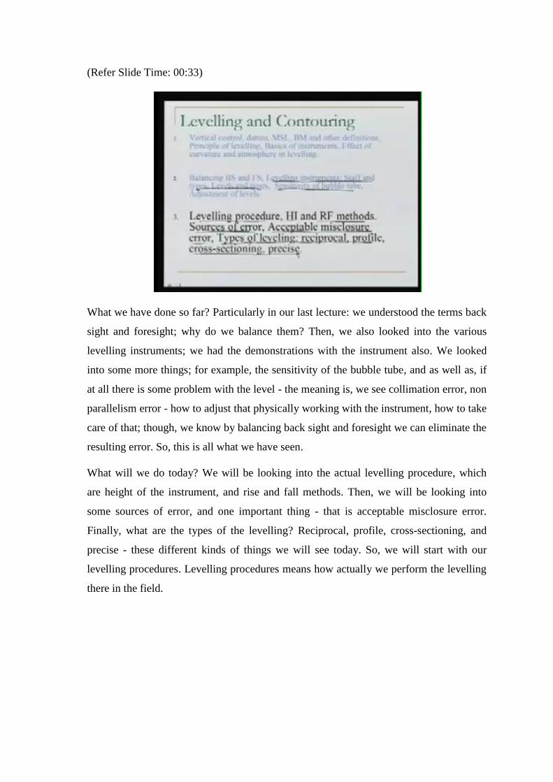
What have we understood so far? We have understood well, if there is some ground, we
keep our level, the staff at these two points and by making a horizontal line of sight,
because we can only make a horizontal line of sight - not exactly horizontal because that
is affected by the refraction. Using this horizontal line of sight - for a small area, we can
say horizontal - we determine the readings Ra and Rb. Then, if I know this particular
value - the RL of this point - I can compute the RL of this point. So, this is what we have
understood; but, actually how do we implement this thing in field? This is important. So,
this is what we are going to do now.
(Refer Slide Time: 02:45)
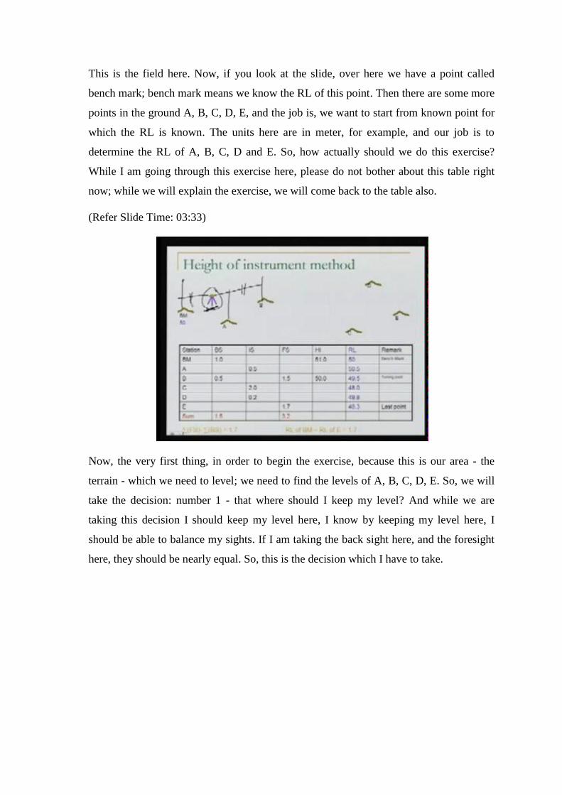
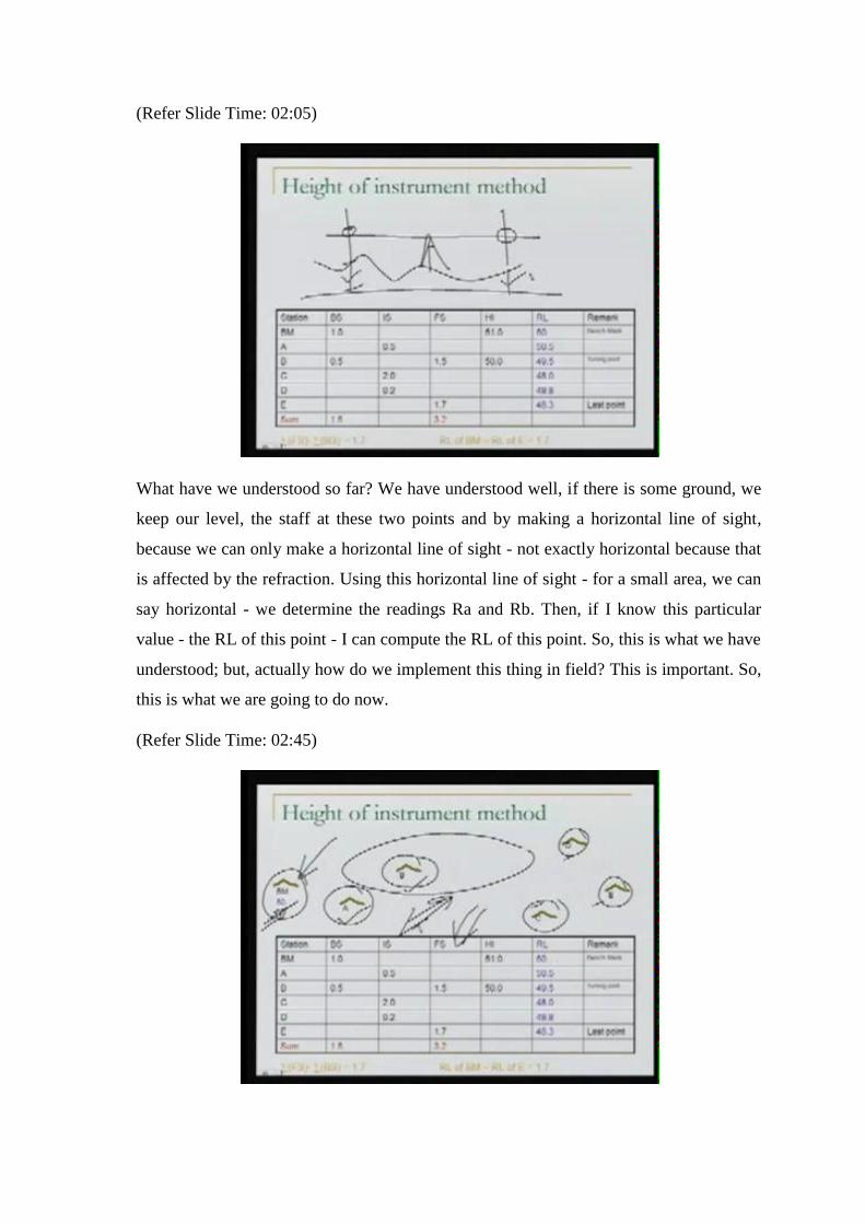
This is the field here. Now, if you look at the slide, over here we have a point called
bench mark; bench mark means we know the RL of this point. Then there are some more
points in the ground A, B, C, D, E, and the job is, we want to start from known point for
which the RL is known. The units here are in meter, for example, and our job is to
determine the RL of A, B, C, D and E. So, how actually should we do this exercise?
While I am going through this exercise here, please do not bother about this table right
now; while we will explain the exercise, we will come back to the table also.
(Refer Slide Time: 03:33)
Now, the very first thing, in order to begin the exercise, because this is our area - the
terrain - which we need to level; we need to find the levels of A, B, C, D, E. So, we will
take the decision: number 1 - that where should I keep my level? And while we are
taking this decision I should keep my level here, I know by keeping my level here, I
should be able to balance my sights. If I am taking the back sight here, and the foresight
here, they should be nearly equal. So, this is the decision which I have to take.
(Refer Slide Time: 04:05)
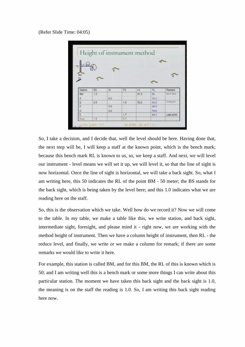
So, I take a decision, and I decide that, well the level should be here. Having done that,
the next step will be, I will keep a staff at the known point, which is the bench mark;
because this bench mark RL is known to us, so, we keep a staff. And next, we will level
our instrument - level means we will set it up, we will level it, so that the line of sight is
now horizontal. Once the line of sight is horizontal, we will take a back sight. So, what I
am writing here, this 50 indicates the RL of the point BM - 50 meter; the BS stands for
the back sight, which is being taken by the level here; and this 1.0 indicates what we are
reading here on the staff.
So, this is the observation which we take. Well how do we record it? Now we will come
to the table. In my table, we make a table like this, we write station, and back sight,
intermediate sight, foresight, and please mind it - right now, we are working with the
method height of instrument. Then we have a column height of instrument, then RL - the
reduce level, and finally, we write or we make a column for remark; if there are some
remarks we would like to write it here.
For example, this station is called BM, and for this BM, the RL of this is known which is
50; and I am writing well this is a bench mark or some more things I can write about this
particular station. The moment we have taken this back sight and the back sight is 1.0,
the meaning is on the staff the reading is 1.0. So, I am writing this back sight reading
here now.
So far, just do not bother about any of these things; all of these are just blank; just do not
bother about these. We are only bothering about right now, in this empty table, I have
filled it only here. So, I am writing this 1.0.
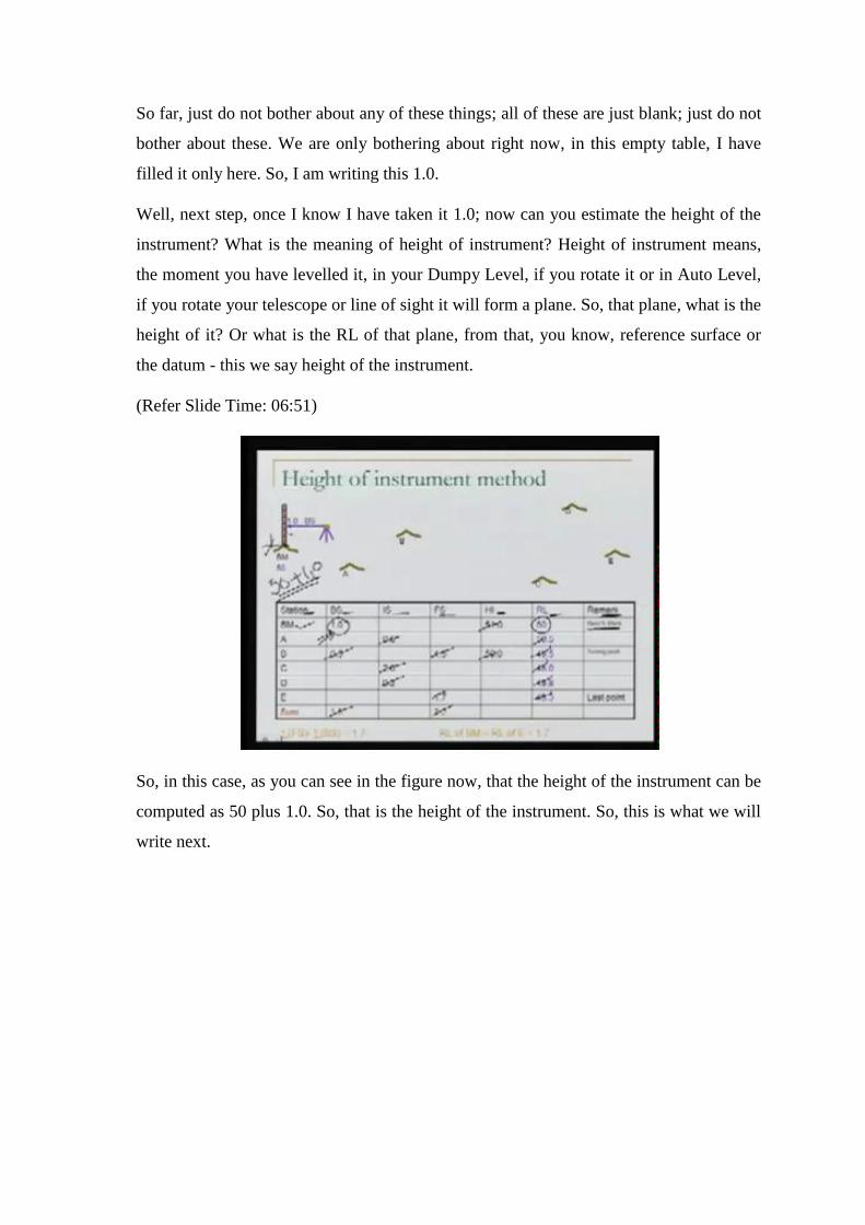
Well, next step, once I know I have taken it 1.0; now can you estimate the height of the
instrument? What is the meaning of height of instrument? Height of instrument means,
the moment you have levelled it, in your Dumpy Level, if you rotate it or in Auto Level,
if you rotate your telescope or line of sight it will form a plane. So, that plane, what is the
height of it? Or what is the RL of that plane, from that, you know, reference surface or
the datum - this we say height of the instrument.
(Refer Slide Time: 06:51)
So, in this case, as you can see in the figure now, that the height of the instrument can be
computed as 50 plus 1.0. So, that is the height of the instrument. So, this is what we will
write next.
(Refer Slide Time: 07:02)
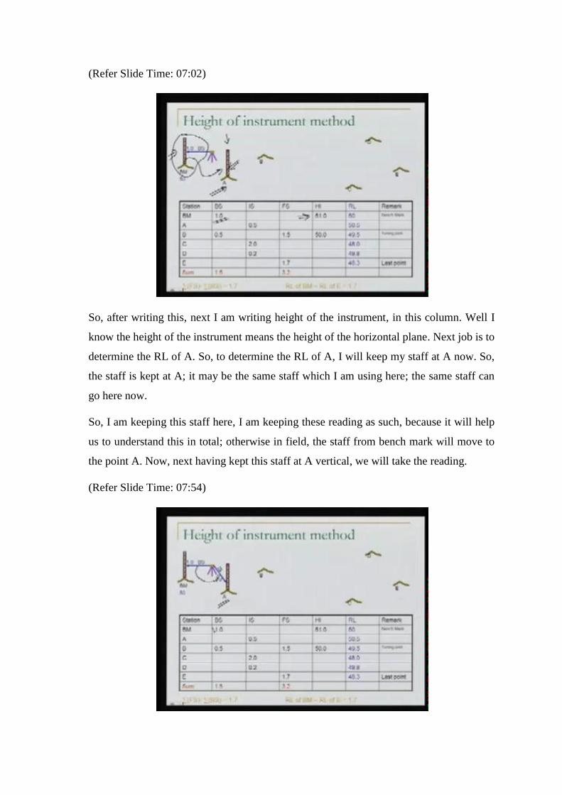
So, after writing this, next I am writing height of the instrument, in this column. Well I
know the height of the instrument means the height of the horizontal plane. Next job is to
determine the RL of A. So, to determine the RL of A, I will keep my staff at A now. So,
the staff is kept at A; it may be the same staff which I am using here; the same staff can
go here now.
So, I am keeping this staff here, I am keeping these reading as such, because it will help
us to understand this in total; otherwise in field, the staff from bench mark will move to
the point A. Now, next having kept this staff at A vertical, we will take the reading.
(Refer Slide Time: 07:54)
And what I have done in this case? This line does not seem to be horizontal, but does not
matter. I just rotated my level in a horizontal plane. And we know it; once we rotate the
level in a horizontal plane, the line of sight will still be horizontal. So, right now, I am
bisecting the staff at A, and still my line of sight is horizontal, and I take one observation
here, and this observation is 0.5.
(Refer Slide Time: 08:23)
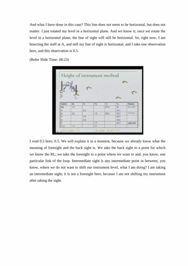
I read 0.5 here; 0.5. We will explain it in a moment, because we already know what the
meaning of foresight and the back sight is. We take the back sight to a point for which
we know the RL; we take the foresight to a point where we want to and, you know, one
particular link of the loop. Intermediate sight is any intermediate point in between, you
know, where we do not want to shift our instrument level, what I am doing? I am taking
an intermediate sight; it is not a foresight here, because I am not shifting my instrument
after taking the sight.
(Refer Slide Time: 09:12)
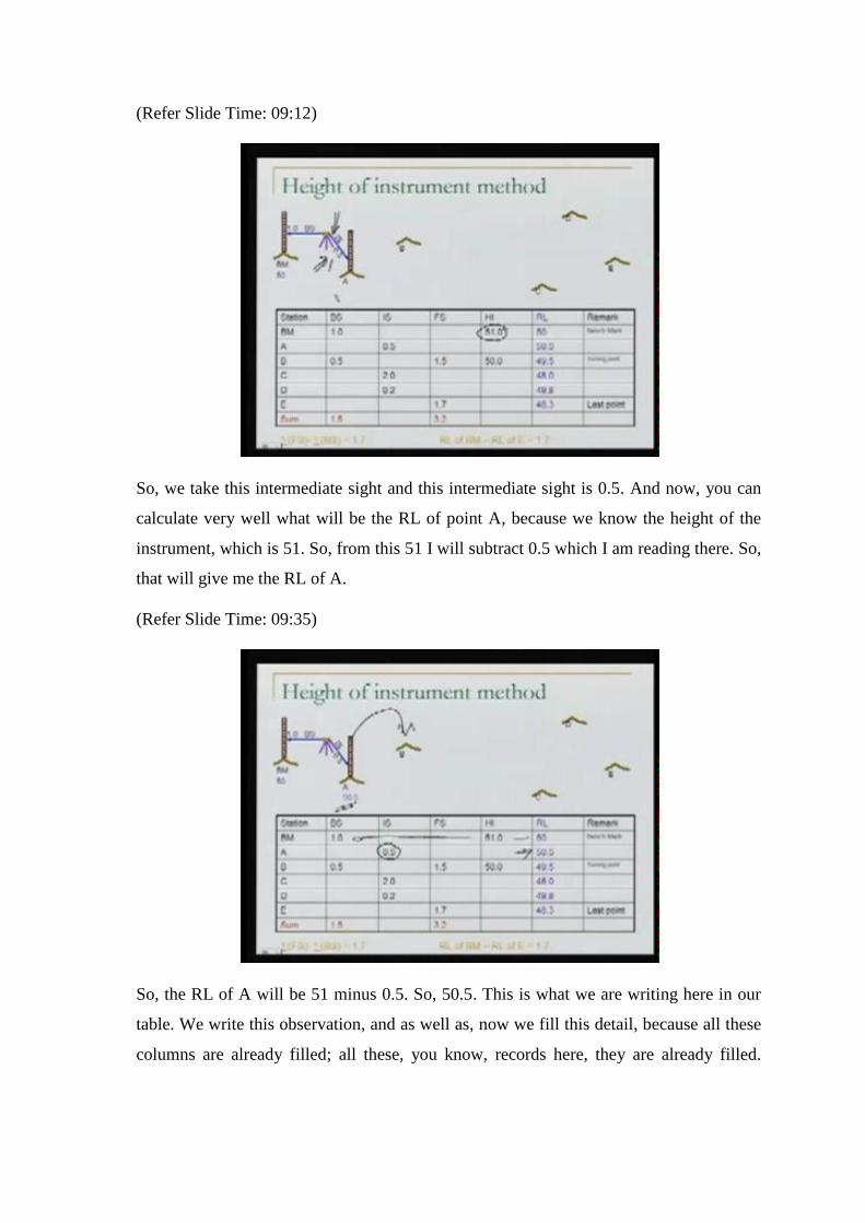
So, we take this intermediate sight and this intermediate sight is 0.5. And now, you can
calculate very well what will be the RL of point A, because we know the height of the
instrument, which is 51. So, from this 51 I will subtract 0.5 which I am reading there. So,
that will give me the RL of A.
(Refer Slide Time: 09:35)
So, the RL of A will be 51 minus 0.5. So, 50.5. This is what we are writing here in our
table. We write this observation, and as well as, now we fill this detail, because all these
columns are already filled; all these, you know, records here, they are already filled.
Well next, our job is to determine the RS of other points. We shift our staff to B. Let us
do it.
(Refer Slide Time: 10:06)
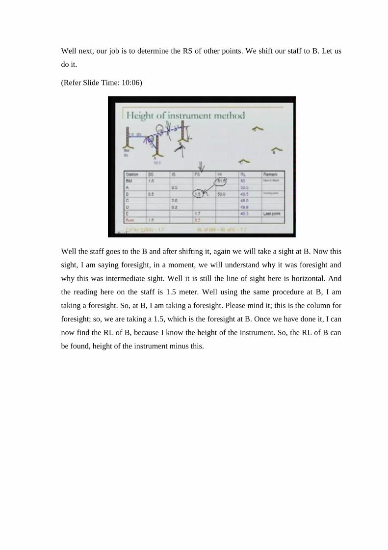
Well the staff goes to the B and after shifting it, again we will take a sight at B. Now this
sight, I am saying foresight, in a moment, we will understand why it was foresight and
why this was intermediate sight. Well it is still the line of sight here is horizontal. And
the reading here on the staff is 1.5 meter. Well using the same procedure at B, I am
taking a foresight. So, at B, I am taking a foresight. Please mind it; this is the column for
foresight; so, we are taking a 1.5, which is the foresight at B. Once we have done it, I can
now find the RL of B, because I know the height of the instrument. So, the RL of B can
be found, height of the instrument minus this.
(Refer Slide Time: 11:03)
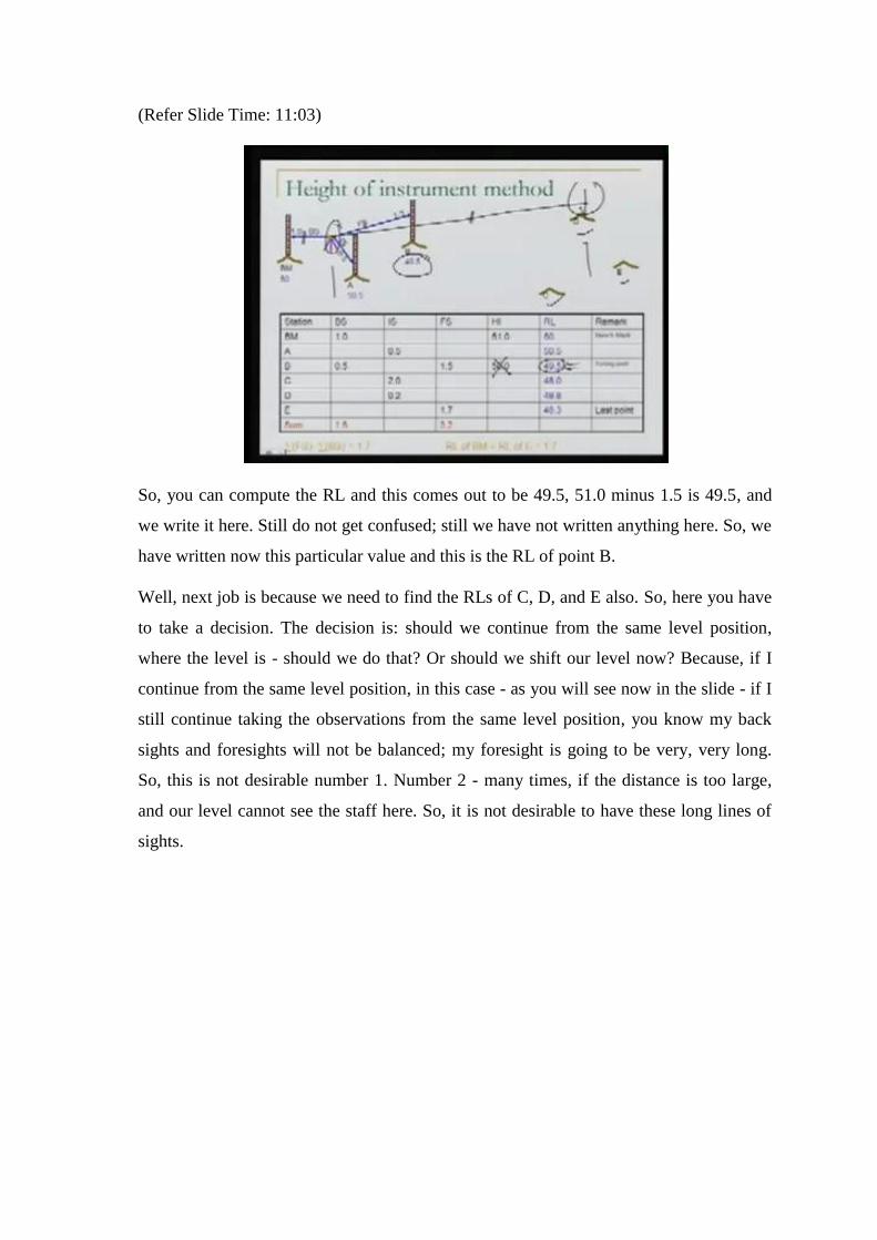
So, you can compute the RL and this comes out to be 49.5, 51.0 minus 1.5 is 49.5, and
we write it here. Still do not get confused; still we have not written anything here. So, we
have written now this particular value and this is the RL of point B.
Well, next job is because we need to find the RLs of C, D, and E also. So, here you have
to take a decision. The decision is: should we continue from the same level position,
where the level is - should we do that? Or should we shift our level now? Because, if I
continue from the same level position, in this case - as you will see now in the slide - if I
still continue taking the observations from the same level position, you know my back
sights and foresights will not be balanced; my foresight is going to be very, very long.
So, this is not desirable number 1. Number 2 - many times, if the distance is too large,
and our level cannot see the staff here. So, it is not desirable to have these long lines of
sights.
(Refer Slide Time: 12:22)
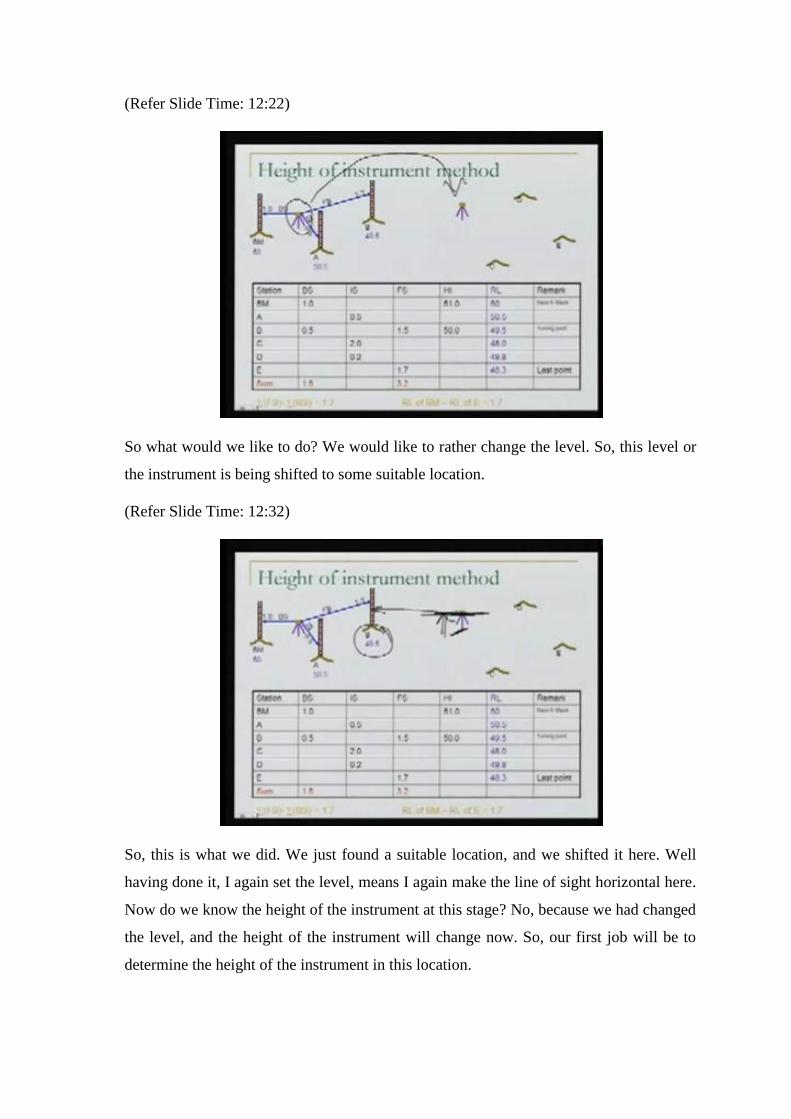
So what would we like to do? We would like to rather change the level. So, this level or
the instrument is being shifted to some suitable location.
(Refer Slide Time: 12:32)
So, this is what we did. We just found a suitable location, and we shifted it here. Well
having done it, I again set the level, means I again make the line of sight horizontal here.
Now do we know the height of the instrument at this stage? No, because we had changed
the level, and the height of the instrument will change now. So, our first job will be to
determine the height of the instrument in this location.
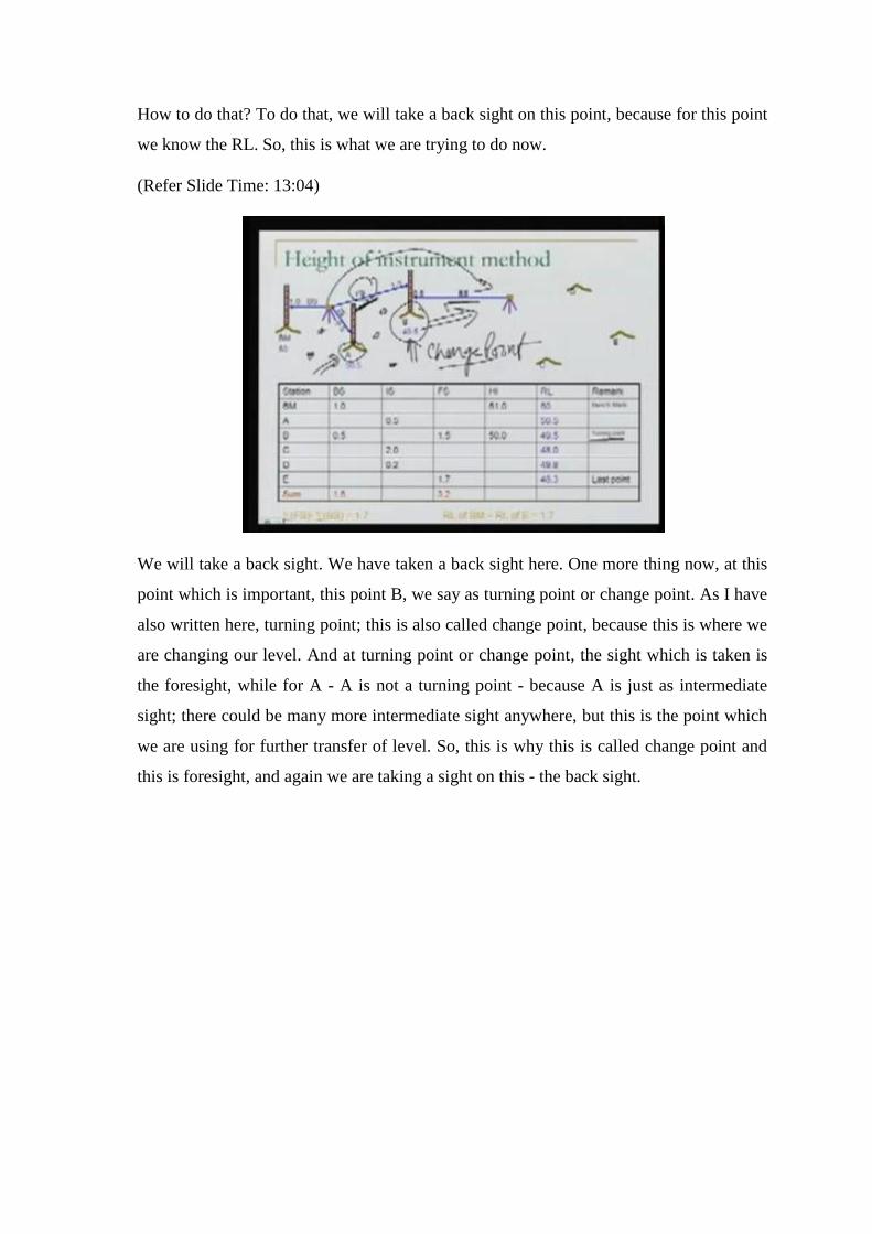
How to do that? To do that, we will take a back sight on this point, because for this point
we know the RL. So, this is what we are trying to do now.
(Refer Slide Time: 13:04)
We will take a back sight. We have taken a back sight here. One more thing now, at this
point which is important, this point B, we say as turning point or change point. As I have
also written here, turning point; this is also called change point, because this is where we
are changing our level. And at turning point or change point, the sight which is taken is
the foresight, while for A - A is not a turning point - because A is just as intermediate
sight; there could be many more intermediate sight anywhere, but this is the point which
we are using for further transfer of level. So, this is why this is called change point and
this is foresight, and again we are taking a sight on this - the back sight.
(Refer Slide Time: 13:59)
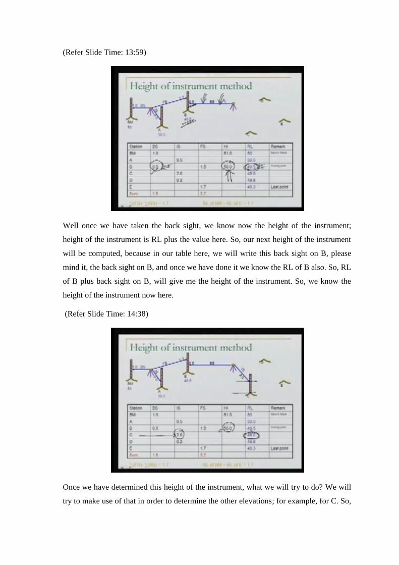
Well once we have taken the back sight, we know now the height of the instrument;
height of the instrument is RL plus the value here. So, our next height of the instrument
will be computed, because in our table here, we will write this back sight on B, please
mind it, the back sight on B, and once we have done it we know the RL of B also. So, RL
of B plus back sight on B, will give me the height of the instrument. So, we know the
height of the instrument now here.
(Refer Slide Time: 14:38)
Once we have determined this height of the instrument, what we will try to do? We will
try to make use of that in order to determine the other elevations; for example, for C. So,
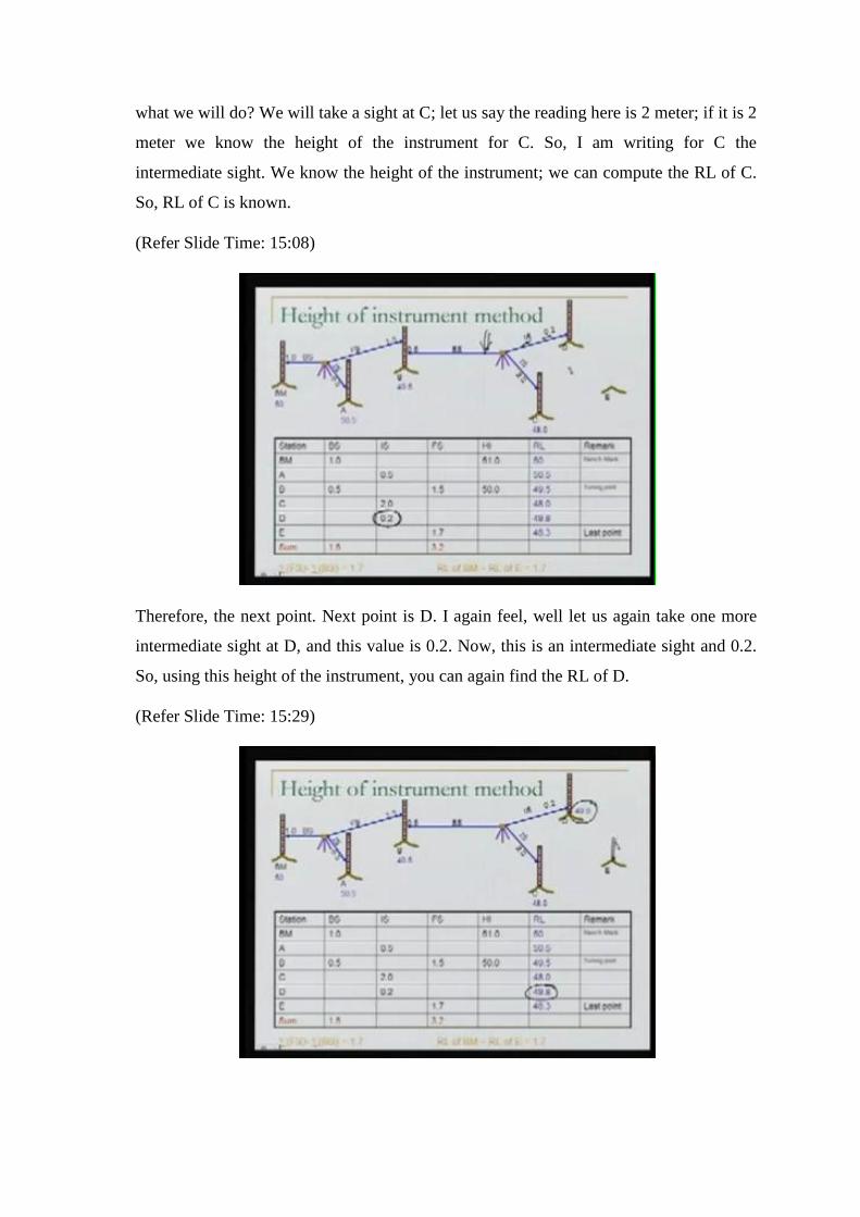
what we will do? We will take a sight at C; let us say the reading here is 2 meter; if it is 2
meter we know the height of the instrument for C. So, I am writing for C the
intermediate sight. We know the height of the instrument; we can compute the RL of C.
So, RL of C is known.
(Refer Slide Time: 15:08)
Therefore, the next point. Next point is D. I again feel, well let us again take one more
intermediate sight at D, and this value is 0.2. Now, this is an intermediate sight and 0.2.
So, using this height of the instrument, you can again find the RL of D.
(Refer Slide Time: 15:29)
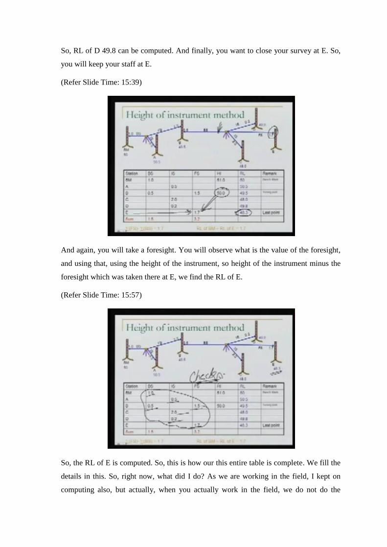
So, RL of D 49.8 can be computed. And finally, you want to close your survey at E. So,
you will keep your staff at E.
(Refer Slide Time: 15:39)
And again, you will take a foresight. You will observe what is the value of the foresight,
and using that, using the height of the instrument, so height of the instrument minus the
foresight which was taken there at E, we find the RL of E.
(Refer Slide Time: 15:57)
So, the RL of E is computed. So, this is how our this entire table is complete. We fill the
details in this. So, right now, what did I do? As we are working in the field, I kept on
computing also, but actually, when you actually work in the field, we do not do the
computations there; rather we just keep recording, as you can see in the slide here, only
the back sight, intermediate sight, foresight, back sight, intermediate sight, intermediate
sight, foresight - this is what only we record; nothing else; the rest of the table or rest of
the computations are done later on, in the laboratory.
(Refer Slide Time: 16:48)
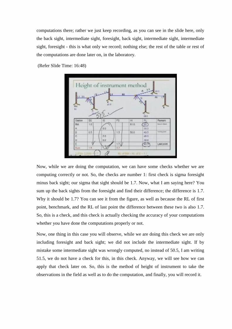
Now, while we are doing the computation, we can have some checks whether we are
computing correctly or not. So, the checks are number 1: first check is sigma foresight
minus back sight; our sigma that sight should be 1.7. Now, what I am saying here? You
sum up the back sights from the foresight and find their difference; the difference is 1.7.
Why it should be 1.7? You can see it from the figure, as well as because the RL of first
point, benchmark, and the RL of last point the difference between these two is also 1.7.
So, this is a check, and this check is actually checking the accuracy of your computations
whether you have done the computations properly or not.
Now, one thing in this case you will observe, while we are doing this check we are only
including foresight and back sight; we did not include the intermediate sight. If by
mistake some intermediate sight was wrongly computed, no instead of 50.5, I am writing
51.5, we do not have a check for this, in this check. Anyway, we will see how we can
apply that check later on. So, this is the method of height of instrument to take the
observations in the field as well as to do the computation, and finally, you will record it.
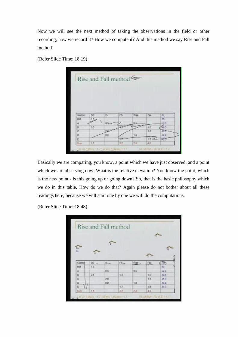
Now we will see the next method of taking the observations in the field or other
recording, how we record it? How we compute it? And this method we say Rise and Fall
method.
(Refer Slide Time: 18:19)
Basically we are comparing, you know, a point which we have just observed, and a point
which we are observing now. What is the relative elevation? You know the point, which
is the new point - is this going up or going down? So, that is the basic philosophy which
we do in this table. How do we do that? Again please do not bother about all these
readings here, because we will start one by one we will do the computations.
(Refer Slide Time: 18:48)
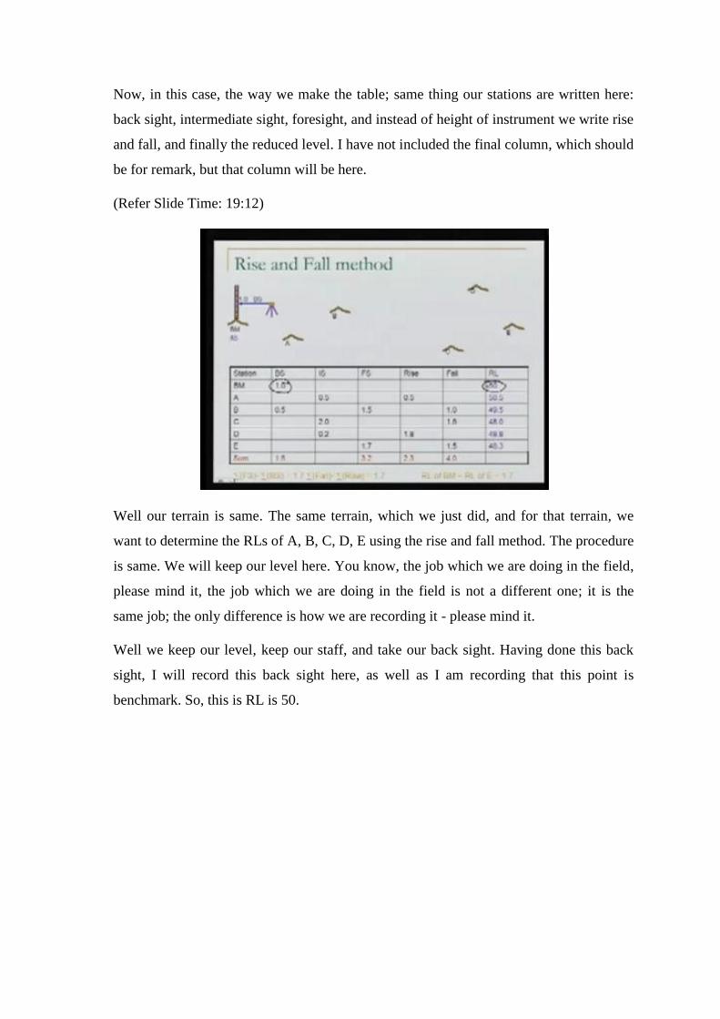
Now, in this case, the way we make the table; same thing our stations are written here:
back sight, intermediate sight, foresight, and instead of height of instrument we write rise
and fall, and finally the reduced level. I have not included the final column, which should
be for remark, but that column will be here.
(Refer Slide Time: 19:12)
Well our terrain is same. The same terrain, which we just did, and for that terrain, we
want to determine the RLs of A, B, C, D, E using the rise and fall method. The procedure
is same. We will keep our level here. You know, the job which we are doing in the field,
please mind it, the job which we are doing in the field is not a different one; it is the
same job; the only difference is how we are recording it - please mind it.
Well we keep our level, keep our staff, and take our back sight. Having done this back
sight, I will record this back sight here, as well as I am recording that this point is
benchmark. So, this is RL is 50.
(Refer Slide Time: 19:55)
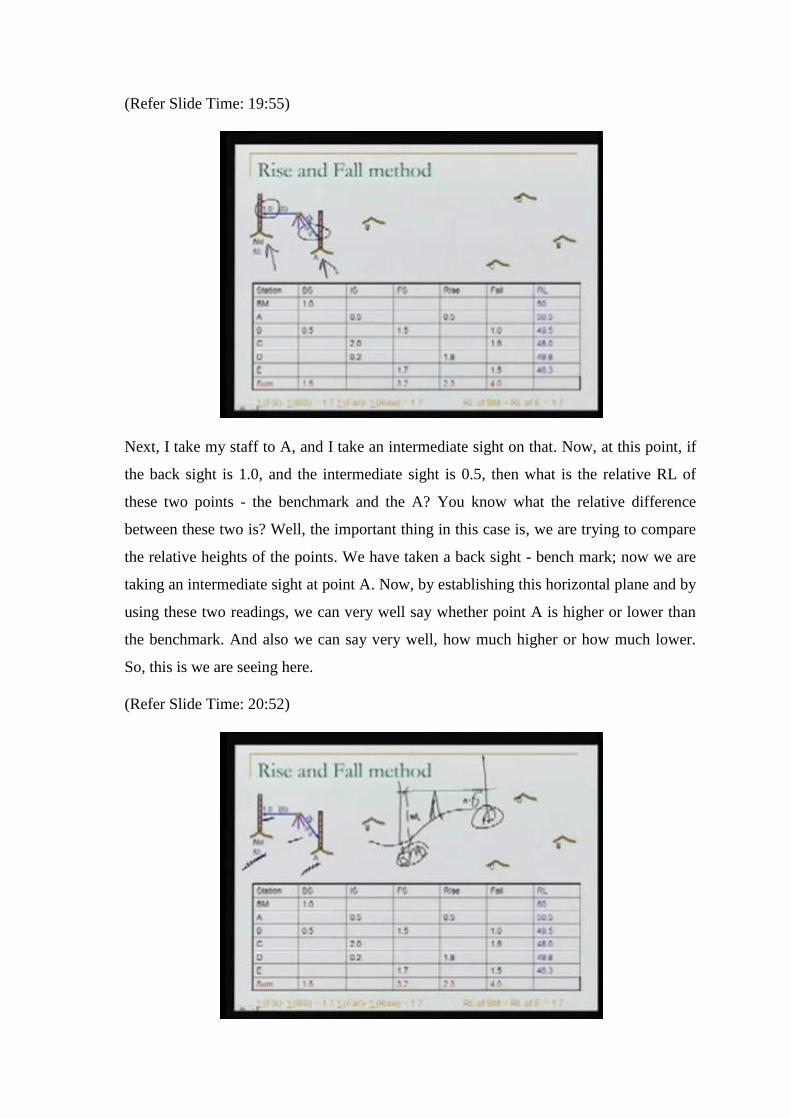
Next, I take my staff to A, and I take an intermediate sight on that. Now, at this point, if
the back sight is 1.0, and the intermediate sight is 0.5, then what is the relative RL of
these two points - the benchmark and the A? You know what the relative difference
between these two is? Well, the important thing in this case is, we are trying to compare
the relative heights of the points. We have taken a back sight - bench mark; now we are
taking an intermediate sight at point A. Now, by establishing this horizontal plane and by
using these two readings, we can very well say whether point A is higher or lower than
the benchmark. And also we can say very well, how much higher or how much lower.
So, this is we are seeing here.
(Refer Slide Time: 20:52)
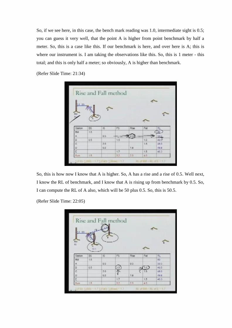
So, if we see here, in this case, the bench mark reading was 1.0, intermediate sight is 0.5;
you can guess it very well, that the point A is higher from point benchmark by half a
meter. So, this is a case like this. If our benchmark is here, and over here is A; this is
where our instrument is. I am taking the observations like this. So, this is 1 meter - this
total; and this is only half a meter; so obviously, A is higher than benchmark.
(Refer Slide Time: 21:34)
So, this is how now I know that A is higher. So, A has a rise and a rise of 0.5. Well next,
I know the RL of benchmark, and I know that A is rising up from benchmark by 0.5. So,
I can compute the RL of A also, which will be 50 plus 0.5. So, this is 50.5.
(Refer Slide Time: 22:05)
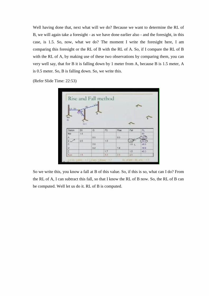
Well having done that, next what will we do? Because we want to determine the RL of
B, we will again take a foresight - as we have done earlier also - and the foresight, in this
case, is 1.5. So, now, what we do? The moment I write the foresight here, I am
comparing this foresight or the RL of B with the RL of A. So, if I compare the RL of B
with the RL of A, by making use of these two observations by comparing them, you can
very well say, that for B it is falling down by 1 meter from A, because B is 1.5 meter, A
is 0.5 meter. So, B is falling down. So, we write this.
(Refer Slide Time: 22:53)
So we write this, you know a fall at B of this value. So, if this is so, what can I do? From
the RL of A, I can subtract this fall, so that I know the RL of B now. So, the RL of B can
be computed. Well let us do it. RL of B is computed.
(Refer Slide Time: 23:11)
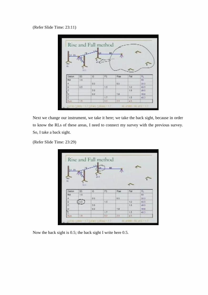
Next we change our instrument, we take it here; we take the back sight, because in order
to know the RLs of these areas, I need to connect my survey with the previous survey.
So, I take a back sight.
(Refer Slide Time: 23:29)
Now the back sight is 0.5; the back sight I write here 0.5.
(Refer Slide Time: 23:41)
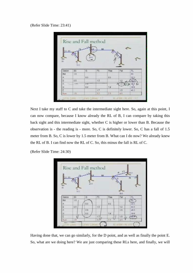
Next I take my staff to C and take the intermediate sight here. So, again at this point, I
can now compare, because I know already the RL of B, I can compare by taking this
back sight and this intermediate sight, whether C is higher or lower than B. Because the
observation is - the reading is - more. So, C is definitely lower. So, C has a fall of 1.5
meter from B. So, C is lower by 1.5 meter from B. What can I do now? We already knew
the RL of B. I can find now the RL of C. So, this minus the fall is RL of C.
(Refer Slide Time: 24:30)
Having done that, we can go similarly, for the D point, and as well as finally the point E.
So, what are we doing here? We are just comparing these RLs here, and finally, we will
write all these observations. Now in this case, as we will see in a moment, we can apply
some extra checks. What these checks are we will see now in the slide.
Well the very first check is RL of first point minus RL of last point is 1.7. Well we have
already done it - sigma of back sight minus sigma of foresight, this is 1.7; we have done
it already. One more check that we can do, because you know, we are either rising up or
falling down. So, the sum of rise and sum of fall, they should also - if you find the
difference of these two that should be same as how much the first point is higher or
lower than the last point. So, this is what we are doing here; we will find sum of rise,
sum of fall, and find their difference, and this difference also comes out to be 1.7. So,
what we have done? We have now, unlike the previous method - the method of height of
the instrument, we have also now… you know, because in rise and fall the way we are
computing them, we are including the intermediate sight also.
So, you know, we are applying this correction now or applying this check to the
intermediate sights also. If any of the intermediate sight computation is done wrongly,
we can have a check here now. So in that respect this is better method.
(Refer Slide Time: 26:18)
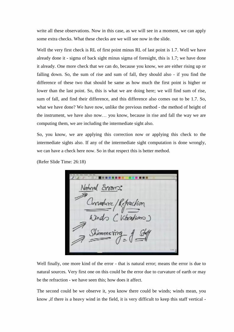
Well finally, one more kind of the error - that is natural error; means the error is due to
natural sources. Very first one on this could be the error due to curvature of earth or may
be the refraction - we have seen this; how does it affect.
The second could be we observe it, you know there could be winds; winds mean, you
know ,if there is a heavy wind in the field, it is very difficult to keep this staff vertical -
number one. Number two sometime also, it may happen that your instrument may have
some vibrations, because of that there will be problem.
Now, finally, the third one, and you can experience this only if you are looking through
the telescope; please do that - look through the telescope at a you know staff which is
kept at 100 meter, 150 meter, you know, far away. What you will observe, particularly
during the summers, because of different layers in atmosphere and their relative
movement the image of this staff appears as if it is shimmering. So, it becomes very
difficult if the staff is shimmering to bisect a point there, and this leads to again some
error.
Now we have seen all these different kinds of the errors which may occur in levelling,
but what we saw only a few of those. There may be various different kinds of sources
and that you will experience more when you are in the field.
Now what we will do? We will talk about the types of levelling. Now, what is the
meaning of types of levelling? Types of levelling means we have seen, this simple way,
you know, how the levelling can be done, but actually some categories are there, and we
specifically would like to name them, and how do we do levelling in those categories -
this is what we are going to discuss now. In the type of levelling, we will start with the
very first one, which we say, Reciprocal levelling.
(Refer Slide Time: 28:29)
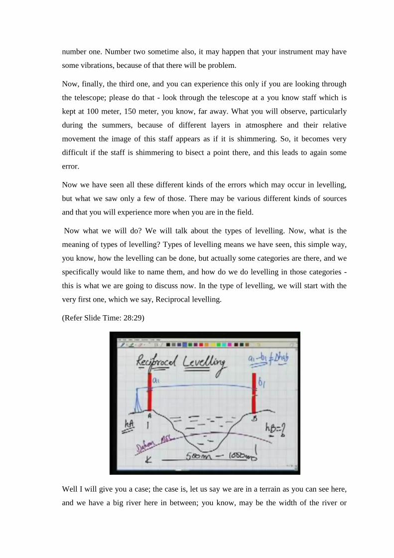
Well I will give you a case; the case is, let us say we are in a terrain as you can see here,
and we have a big river here in between; you know, may be the width of the river or
between these two points the distance is 500 meter, or may be 1 kilometer. You know,
these two points A and B are very far apart - 200, 300, 400 whatever. Then in addition to
this there is a problem now, because we know somehow the RL of A. So, ha is known to
us and we want to determine hb. Well how to do that? If you are using the split level or
the levelling instruments, how to perform this exercise? That we have to see now.
We know in order to eliminate the effect of errors in the instrument - levelling instrument
- as well as the zero error we saw for the staff, or also for the curvature error, refraction
error, in all these cases if we balance the back sight and foresight, these errors can be
eliminated; but balancing back sight and foresight, here in this case, is not possible. So,
we cannot keep our level here in between.
So, what to do in that case? We cannot keep our level here. If I keep my level only on
one sight, you know like this, and I take the observation; somewhere here I read. If I take
observation a1 and here b1, a1 minus b1 will not give me delta hab - the difference in
elevation between A and B; it will not give me, because of the errors; we know that
already. Now, how to eliminate that?
(Refer Slide Time: 30:22)
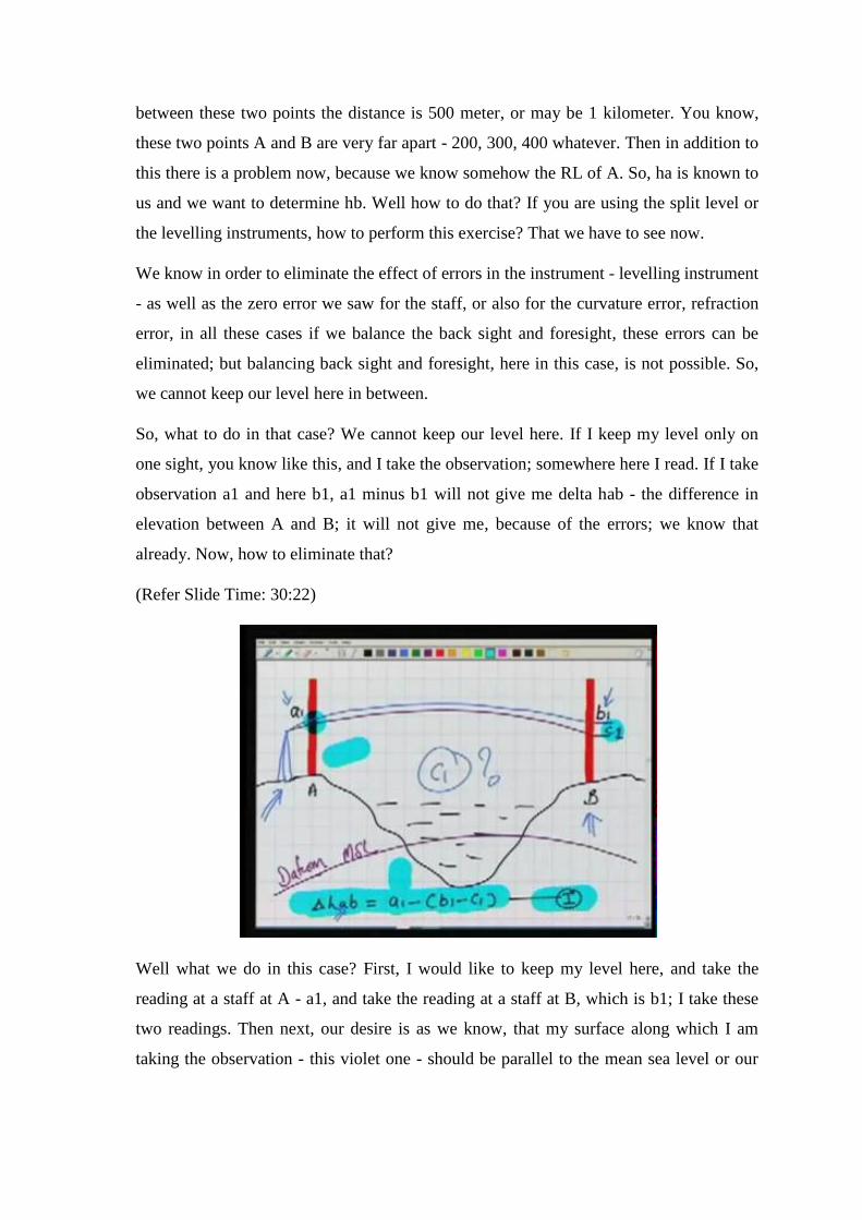
Well what we do in this case? First, I would like to keep my level here, and take the
reading at a staff at A - a1, and take the reading at a staff at B, which is b1; I take these
two readings. Then next, our desire is as we know, that my surface along which I am
taking the observation - this violet one - should be parallel to the mean sea level or our
datum; this is what our desire is, but this is not be the case; we know it. We try to make
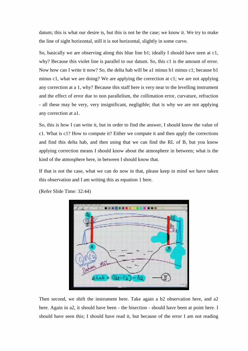
the line of sight horizontal, still it is not horizontal, slightly in some curve.
So, basically we are observing along this blue line b1; ideally I should have seen at c1,
why? Because this violet line is parallel to our datum. So, this c1 is the amount of error.
Now how can I write it now? So, the delta hab will be a1 minus b1 minus c1; because b1
minus c1, what we are doing? We are applying the correction at c1; we are not applying
any correction at a 1, why? Because this staff here is very near to the levelling instrument
and the effect of error due to non parallelism, the collimation error, curvature, refraction
- all these may be very, very insignificant, negligible; that is why we are not applying
any correction at a1.
So, this is how I can write it, but in order to find the answer, I should know the value of
c1. What is c1? How to compute it? Either we compute it and then apply the corrections
and find this delta hab, and then using that we can find the RL of B, but you know
applying correction means I should know about the atmosphere in between; what is the
kind of the atmosphere here, in between I should know that.
If that is not the case, what we can do now in that, please keep in mind we have taken
this observation and I am writing this as equation 1 here.
(Refer Slide Time: 32:44)
Then second, we shift the instrument here. Take again a b2 observation here, and a2
here. Again in a2, it should have been - the bisection - should have been at point here. I
should have seen this; I should have read it, but because of the error I am not reading
this, but I am rather, I am reading somewhere here at a2. So, I should apply in a2 the
correction which is equal to c2. So, this is what I am trying to do now. What we are
doing here, you know, the difference in elevation between A and B delta hab, I am
writing for this case as a2 minus c2, because whatever I am reading at a2, I am applying
correction to that, minus b2; no correction at b2, because the staff at B is very near to the
instrument.
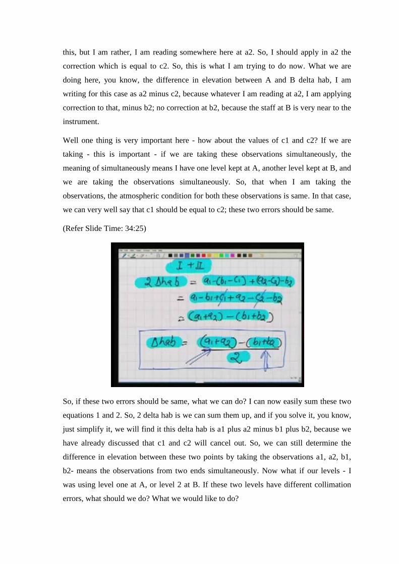
Well one thing is very important here - how about the values of c1 and c2? If we are
taking - this is important - if we are taking these observations simultaneously, the
meaning of simultaneously means I have one level kept at A, another level kept at B, and
we are taking the observations simultaneously. So, that when I am taking the
observations, the atmospheric condition for both these observations is same. In that case,
we can very well say that c1 should be equal to c2; these two errors should be same.
(Refer Slide Time: 34:25)
So, if these two errors should be same, what we can do? I can now easily sum these two
equations 1 and 2. So, 2 delta hab is we can sum them up, and if you solve it, you know,
just simplify it, we will find it this delta hab is a1 plus a2 minus b1 plus b2, because we
have already discussed that c1 and c2 will cancel out. So, we can still determine the
difference in elevation between these two points by taking the observations a1, a2, b1,
b2- means the observations from two ends simultaneously. Now what if our levels - I
was using level one at A, or level 2 at B. If these two levels have different collimation
errors, what should we do? What we would like to do?
(Refer Slide Time: 35:22)
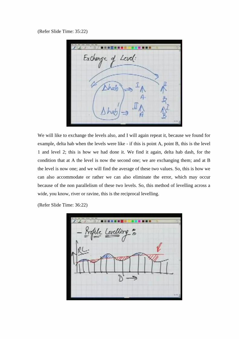
We will like to exchange the levels also, and I will again repeat it, because we found for
example, delta hab when the levels were like - if this is point A, point B, this is the level
1 and level 2; this is how we had done it. We find it again, delta hab dash, for the
condition that at A the level is now the second one; we are exchanging them; and at B
the level is now one; and we will find the average of these two values. So, this is how we
can also accommodate or rather we can also eliminate the error, which may occur
because of the non parallelism of these two levels. So, this method of levelling across a
wide, you know, river or ravine, this is the reciprocal levelling.
(Refer Slide Time: 36:22)
Now next method of levelling is Profile levelling. Now, these are very simple things;
more about these you can read in any text book, but just to understand these, what these
are? Profile levelling means if you have a ground, and you want to you know, create a
profile of this; profile means for a ground along a distance - distance is D - you want to
know how the RL is varying. You know this is a profile, what a typical profile may look
like this; how the RL is varying? This profile is very important; in many applications if
you are going to, you know, lay a road there, in that particular terrain, you would like to
know the formation level for the road should be such that, that the amount of cutting -
this is cutting, all blue shaded is cutting - should be equal to amount of filling - all this
red shaded is filling.
So, for a kind of optimum solution, the amount of cutting and amount of filling should be
same. How do we know that? You know, we have to construct a road, and before
constructing this, we want to fix the formation level of the road; it should be at this
gradient; and we want to ensure that the amount of the filling and amount of the cutting
should be same. This answer we will get, only if we can do a profile along the road.
(Refer Slide Time: 37:53)
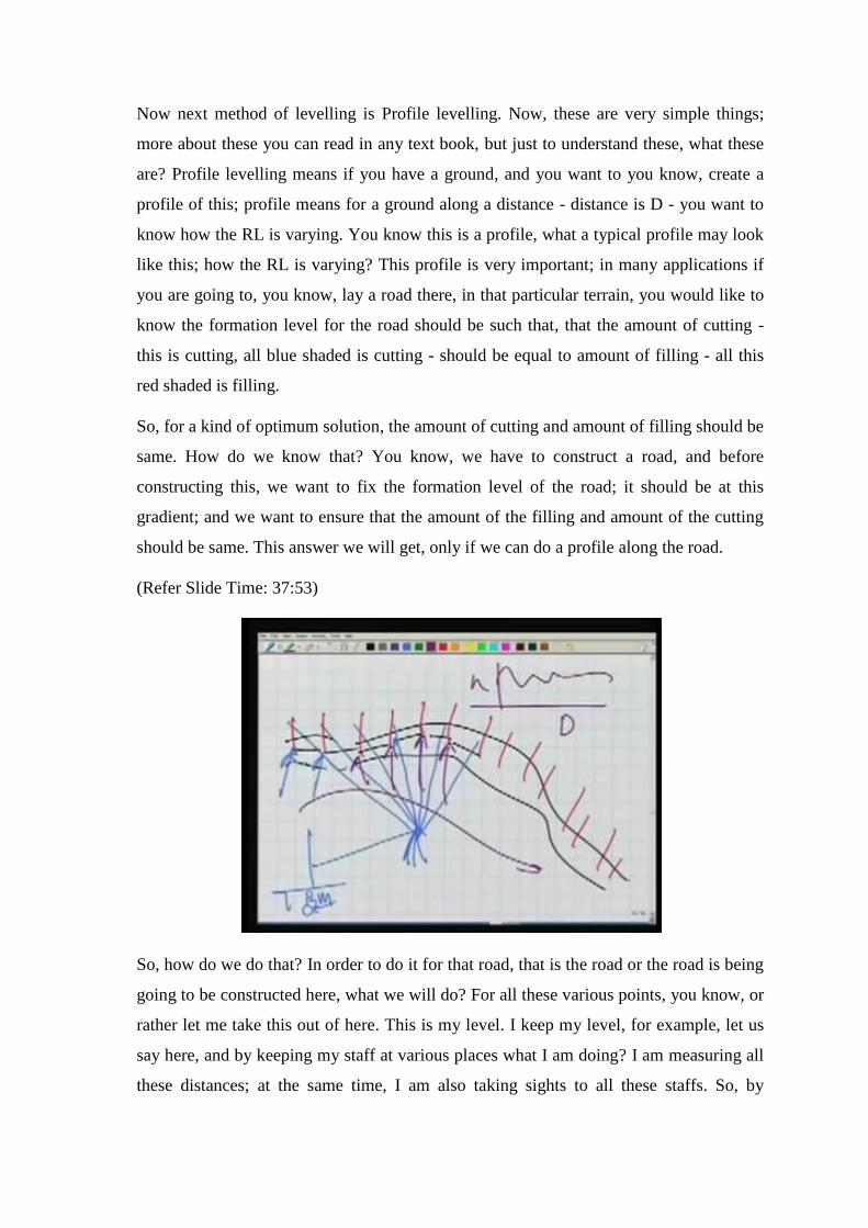
So, how do we do that? In order to do it for that road, that is the road or the road is being
going to be constructed here, what we will do? For all these various points, you know, or
rather let me take this out of here. This is my level. I keep my level, for example, let us
say here, and by keeping my staff at various places what I am doing? I am measuring all
these distances; at the same time, I am also taking sights to all these staffs. So, by
levelling this, and taking this sight also to a benchmark here, I can determine the RLs of
all these points. So, RLs of all these points are known. So, if I know RL of all these
points, I can easily, because I know the distance also along this, I can plot this profile.
And we can use this profile for our application.
(Refer Slide Time: 39:08)
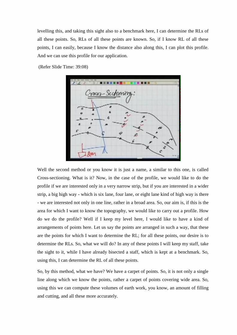
Well the second method or you know it is just a name, a similar to this one, is called
Cross-sectioning. What is it? Now, in the case of the profile, we would like to do the
profile if we are interested only in a very narrow strip, but if you are interested in a wider
strip, a big high way - which is six lane, four lane, or eight lane kind of high way is there
- we are interested not only in one line, rather in a broad area. So, our aim is, if this is the
area for which I want to know the topography, we would like to carry out a profile. How
do we do the profile? Well if I keep my level here, I would like to have a kind of
arrangements of points here. Let us say the points are arranged in such a way, that these
are the points for which I want to determine the RL; for all these points, our desire is to
determine the RLs. So, what we will do? In any of these points I will keep my staff, take
the sight to it, while I have already bisected a staff, which is kept at a benchmark. So,
using this, I can determine the RL of all these points.
So, by this method, what we have? We have a carpet of points. So, it is not only a single
line along which we know the points, rather a carpet of points covering wide area. So,
using this we can compute these volumes of earth work, you know, an amount of filling
and cutting, and all these more accurately.
One more type of levelling is Precise levelling. Precise levelling means, the staff which
were looking at in our last lecture, we said you know the least count is 1 centimeter or
half a centimeter, you know these kind of least count or this kind of staff is not suitable,
or that kind of levelling where we are working with that precision, is not suitable in some
applications. For example, you are interested in laying down the production line in an
industry. Various instruments are being kept along the production line. The centerlines of
those instruments have to match very well; the levels of the instruments, the level of the
foundations, these have to be done very accurately.
Similarly, may be you are interested in, you know, seeing the deflection of a bridge or of
a dam. Again, you look for something which is very, very precise; more accurate
levelling system. This is where we used this Precise levelling. Now in this precise
levelling, how is it done?
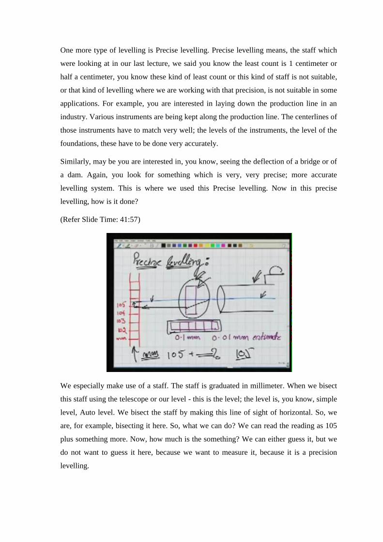
(Refer Slide Time: 41:57)
We especially make use of a staff. The staff is graduated in millimeter. When we bisect
this staff using the telescope or our level - this is the level; the level is, you know, simple
level, Auto level. We bisect the staff by making this line of sight of horizontal. So, we
are, for example, bisecting it here. So, what we can do? We can read the reading as 105
plus something more. Now, how much is the something? We can either guess it, but we
do not want to guess it here, because we want to measure it, because it is a precision
levelling.
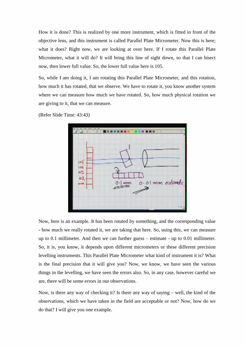
How it is done? This is realized by one more instrument, which is fitted in front of the
objective lens, and this instrument is called Parallel Plate Micrometer. Now this is here;
what it does? Right now, we are looking at over here. If I rotate this Parallel Plate
Micrometer, what it will do? It will bring this line of sight down, so that I can bisect
now, then lower full value. So, the lower full value here is 105.
So, while I am doing it, I am rotating this Parallel Plate Micrometer, and this rotation,
how much it has rotated, that we observe. We have to rotate it, you know another system
where we can measure how much we have rotated. So, how much physical rotation we
are giving to it, that we can measure.
(Refer Slide Time: 43:43)
Now, here is an example. It has been rotated by something, and the corresponding value
- how much we really rotated it, we are taking that here. So, using this, we can measure
up to 0.1 millimeter. And then we can further guess – estimate - up to 0.01 millimeter.
So, it is, you know, it depends upon different micrometers or these different precision
levelling instruments. This Parallel Plate Micrometer what kind of instrument it is? What
is the final precision that it will give you? Now, we know, we have seen the various
things in the levelling, we have seen the errors also. So, in any case, however careful we
are, there will be some errors in our observations.
Now, is there any way of checking it? Is there any way of saying – well, the kind of the
observations, which we have taken in the field are acceptable or not? Now, how do we
do that? I will give you one example.
(Refer Slide Time: 44:39)
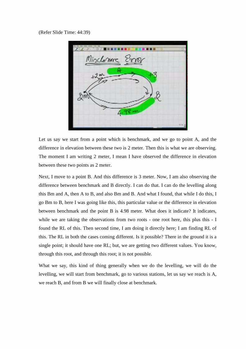
Let us say we start from a point which is benchmark, and we go to point A, and the
difference in elevation between these two is 2 meter. Then this is what we are observing.
The moment I am writing 2 meter, I mean I have observed the difference in elevation
between these two points as 2 meter.
Next, I move to a point B. And this difference is 3 meter. Now, I am also observing the
difference between benchmark and B directly. I can do that. I can do the levelling along
this Bm and A, then A to B, and also Bm and B. And what I found, that while I do this, I
go Bm to B, here I was going like this, this particular value or the difference in elevation
between benchmark and the point B is 4.98 meter. What does it indicate? It indicates,
while we are taking the observations from two roots - one root here, this plus this - I
found the RL of this. Then second time, I am doing it directly here; I am finding RL of
this. The RL in both the cases coming different. Is it possible? There in the ground it is a
single point; it should have one RL; but, we are getting two different values. You know,
through this root, and through this root; it is not possible.
What we say, this kind of thing generally when we do the levelling, we will do the
levelling, we will start from benchmark, go to various stations, let us say we reach is A,
we reach B, and from B we will finally close at benchmark.
(Refer Slide Time: 46:34)
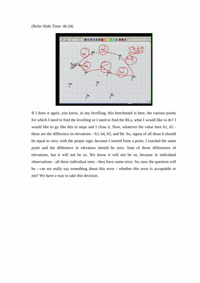
If I draw it again, you know, in any levelling, this benchmark is here, the various points
for which I need to find the levelling or I need to find the RLs, what I would like to do? I
would like to go like this in steps and I close it. Now, whatever the value here h1, h2 -
these are the difference in elevations - h3, h4, h5, and h6. So, sigma of all these h should
be equal to zero, with the proper sign, because I started from a point, I reached the same
point and the difference in elevation should be zero. Sum of those differences of
elevations, but it will not be so. We know it will not be so, because in individual
observations - all these individual ones - they have some error. So, now the question will
be - can we really say something about this error - whether this error is acceptable or
not? We have a way to take this decision.
(Refer Slide Time: 47:34)
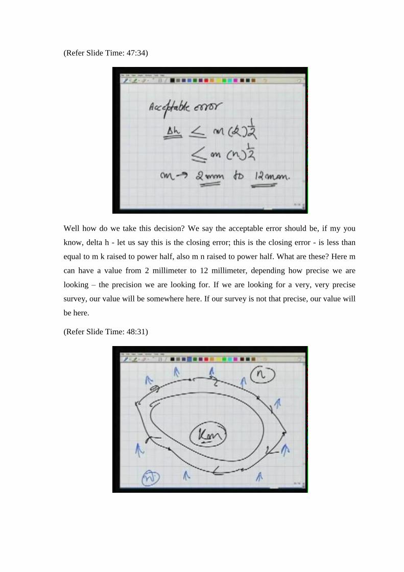
Well how do we take this decision? We say the acceptable error should be, if my you
know, delta h - let us say this is the closing error; this is the closing error - is less than
equal to m k raised to power half, also m n raised to power half. What are these? Here m
can have a value from 2 millimeter to 12 millimeter, depending how precise we are
looking – the precision we are looking for. If we are looking for a very, very precise
survey, our value will be somewhere here. If our survey is not that precise, our value will
be here.
(Refer Slide Time: 48:31)
Now what is k and what is n? k is starting from a point, going to the another point, and
finally, closing our level. This is how we have closed the level. What is the total distance
in kilometer? That is k in this formula. And the n, n stands for when we are doing this
exercise, I might have kept my instrument in several places. You know, how many
settings of the instrument, all these are n. So, we can use either - either the kilometer
thing or the n, and we have to use the same throughout our entire project. So, this is what
the n is - number of the settings of the level instrument; because we know, you know,
more is the kilometer, more will be the error.
(Refer Slide Time: 49:21)
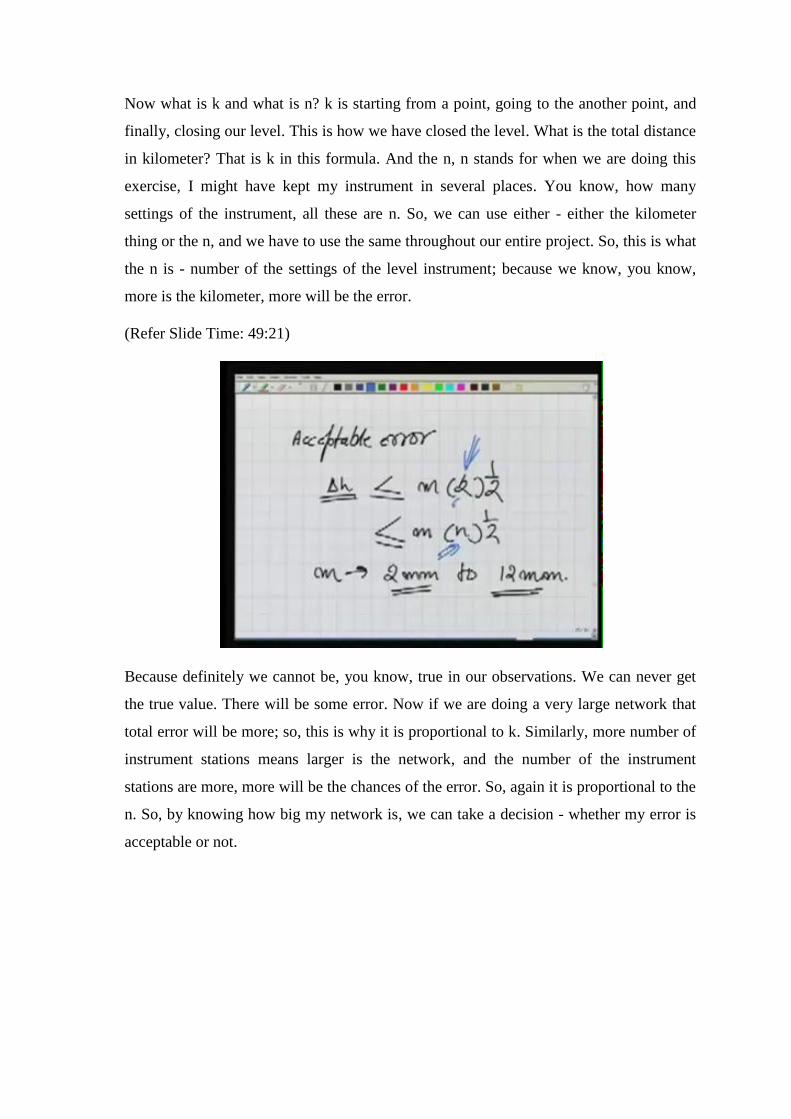
Because definitely we cannot be, you know, true in our observations. We can never get
the true value. There will be some error. Now if we are doing a very large network that
total error will be more; so, this is why it is proportional to k. Similarly, more number of
instrument stations means larger is the network, and the number of the instrument
stations are more, more will be the chances of the error. So, again it is proportional to the
n. So, by knowing how big my network is, we can take a decision - whether my error is
acceptable or not.
(Refer Slide Time: 50:01)
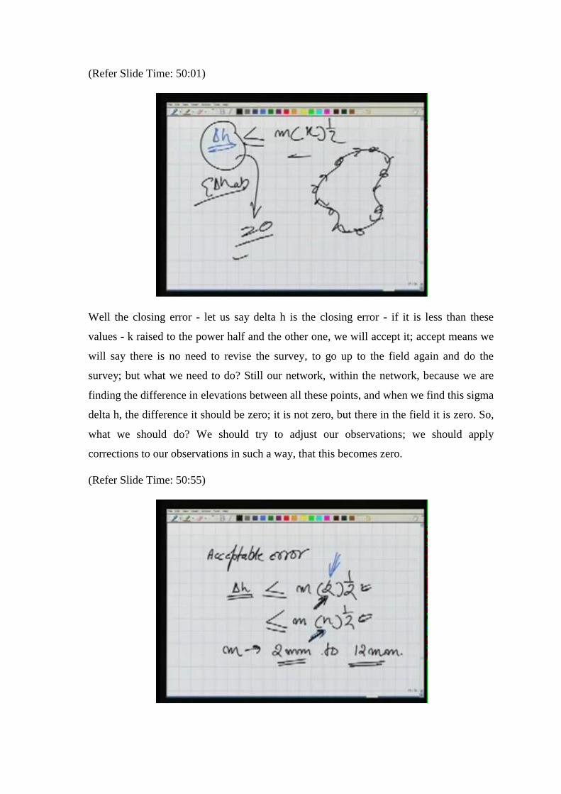
Well the closing error - let us say delta h is the closing error - if it is less than these
values - k raised to the power half and the other one, we will accept it; accept means we
will say there is no need to revise the survey, to go up to the field again and do the
survey; but what we need to do? Still our network, within the network, because we are
finding the difference in elevations between all these points, and when we find this sigma
delta h, the difference it should be zero; it is not zero, but there in the field it is zero. So,
what we should do? We should try to adjust our observations; we should apply
corrections to our observations in such a way, that this becomes zero.
(Refer Slide Time: 50:55)
Now how do we do it? There is a simple method, you know, as we are distributing the
errors - we are distributing the errors or rather we are finding the error, the acceptable
error – parallel, you know, proportional to the distance in kilometer or proportional to the
number of the settings. Similarly, we will try to eliminate the error also, how to apply the
corrections. Well what is the way?
(Refer slide Time: 51:13)
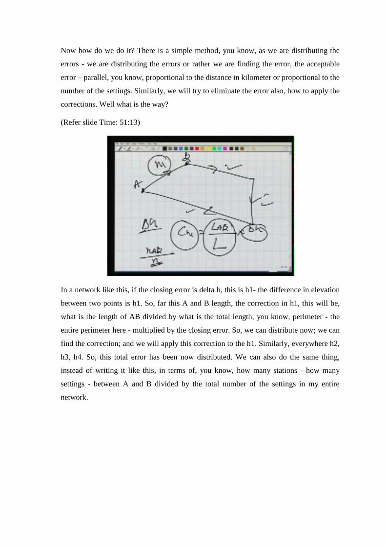
In a network like this, if the closing error is delta h, this is h1- the difference in elevation
between two points is h1. So, far this A and B length, the correction in h1, this will be,
what is the length of AB divided by what is the total length, you know, perimeter - the
entire perimeter here - multiplied by the closing error. So, we can distribute now; we can
find the correction; and we will apply this correction to the h1. Similarly, everywhere h2,
h3, h4. So, this total error has been now distributed. We can also do the same thing,
instead of writing it like this, in terms of, you know, how many stations - how many
settings - between A and B divided by the total number of the settings in my entire
network.
(Refer Slide Time: 52:19)
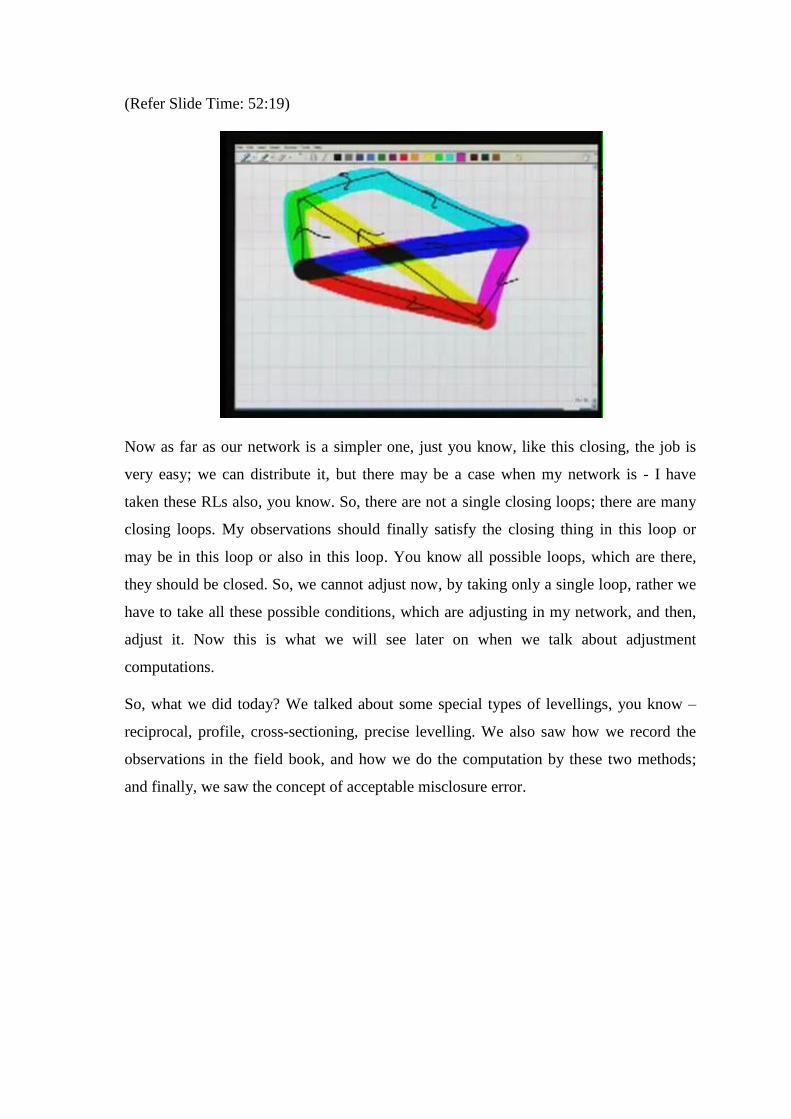
Now as far as our network is a simpler one, just you know, like this closing, the job is
very easy; we can distribute it, but there may be a case when my network is - I have
taken these RLs also, you know. So, there are not a single closing loops; there are many
closing loops. My observations should finally satisfy the closing thing in this loop or
may be in this loop or also in this loop. You know all possible loops, which are there,
they should be closed. So, we cannot adjust now, by taking only a single loop, rather we
have to take all these possible conditions, which are adjusting in my network, and then,
adjust it. Now this is what we will see later on when we talk about adjustment
computations.
So, what we did today? We talked about some special types of levellings, you know –
reciprocal, profile, cross-sectioning, precise levelling. We also saw how we record the
observations in the field book, and how we do the computation by these two methods;
and finally, we saw the concept of acceptable misclosure error.


![Ira A. Fulton College of Engineering | Educating Global ...treedoug/_pages/teaching/ChEn374/Lec24 … · Lec24-Example 2D Square Cylinder Flow over a square cylinder In [35]: # Boi](https://img.pdfslide.net/doc/110x75/603367467dd82505d32c117f/ira-a-fulton-college-of-engineering-educating-global-treedougpagesteachingchen374lec24.jpg)