Embed Size (px)
Citation preview
WELD CLASSIFICATION
BASED ON GREY LEVEL
CO-OCCURRENCE AND
LOCAL BINARY
PATTERNS Master’s Thesis, Global Systems Design
Philip Valentin Study no. 20151784

1
Hand in:
Main report, Test Results and Appendice.
Pages:
Main report: 63 pages
Test results: 31 pages
Appendices: 16 pages
Interview soundfile: https://drive.google.com/open?id=0BxMRnl6eiB0PeDE2YWs1NXFqb0E
Dataset: https://drive.google.com/open?id=0BxMRnl6eiB0PcXJwYi1RdDduazg
Supervisor: Lazaros Nalpantidis
Hand in date: 02-06-2017
2
1 SUMMARY
This project seeks to find a possible solution for the visual examination of welds, where feature extraction
methods are examined and tested with two different classifiers. The idea behind the project is to investigate
if visual inspection based on texture describing features, processed with a machine learning algorithm, can
detect flaws and defects in a weld merely by inspecting the surface of the object.
Visual inspection is the primary way of evaluating weld seams, where construction is not critical and
additional cost is the main risk [1]. Visual inspections entail manual interpretation and evaluation, which are
time consuming, and the result often depends on the person assigned to the task [1], which makes automation
interesting.
The project is based on other research projects regarding the visual inspection of welds and will strive to
devise a solution that can detect one type of defect that is visible to the human eye.
A dataset containing images of both good and bad welds is created from weld samples produced specifically
for this purpose. For preparation of the images, different image processing tools are applied in the making of
the dataset. The dataset is tested on two different feature extraction methods in the search for features that
best explain image textures. To test extracted features, two classification models are tested to find the most
suitable, and their results are discussed. As a result of this, a machine learning algorithm is trained on data
with known targets, and tests on unknown data (processed images) are performed to analyse and compare
results. Several settings, both within feature extraction and classification, are trailed and results are
discussed.
2 ACKNOWLEDGEMENT
At first, I would like to thank my supervisor, Associate Professor Lazaros Nalpantidis of Faculty of
Engineering and Science, Aalborg University. Lazaros guided me through the phases when I ran into
troubles or had questions in general. He kept me on the right track, but still letting the paper be my own.
I would also like to acknowledge Research Assistant Tsampikos Kounalakis of Department of Mechanical
and Manufactural Engineering, Aalborg University who guided towards possible methods and helped me
during technical issues.
I would like thank the expert, Jørgen Melchior from FORCE Technology, who was part of the validation of
the data and provided me with different aspects of similar problems. Without his passionate approach to the
topic and inputs this thesis could not have been successfully conducted.
Philip Valentin

3
3 CONTENTS
1 Summary .................................................................................................................................................... 2
2 Acknowledgement ..................................................................................................................................... 2
4 Preface ....................................................................................................................................................... 5
5 Resumé ...................................................................................................................................................... 6
6 Reading guide ............................................................................................................................................ 7
7 Nomenclature ............................................................................................................................................ 8
8 Introduction ............................................................................................................................................... 9
8.1 Background ...................................................................................................................................... 10
8.2 Problem Statement ........................................................................................................................... 11
8.3 Limitation and Delimitations ........................................................................................................... 12
8.4 Related Work ................................................................................................................................... 13
8.5 State of the Art ................................................................................................................................. 14
9 Methodology ............................................................................................................................................ 15
9.1 Research Design .............................................................................................................................. 15
9.2 Data Collection ................................................................................................................................ 17
9.2.1 Condensed interview ............................................................................................................... 17
9.2.2 Laboratory Tests ...................................................................................................................... 18
9.2.3 Framework ............................................................................................................................... 18
9.3 Quality of Research ......................................................................................................................... 19
10 Literature review ................................................................................................................................. 20
11 Technical Introduction ......................................................................................................................... 24
11.1.1 Welding Robots ....................................................................................................................... 24
11.1.2 Welding Techniques ................................................................................................................ 24
11.1.3 Weld types ............................................................................................................................... 25
11.2 Non-Destructive Testing.................................................................................................................. 25
11.2.1 Visual Inspection of Welds ...................................................................................................... 25
4
11.2.2 Radiographic Testing ............................................................................................................... 26
11.2.3 Ultrasonic Testing.................................................................................................................... 26
12 Methods ............................................................................................................................................... 27
12.1 Image Preparation ............................................................................................................................ 27
12.2 Feature extraction ............................................................................................................................ 27
12.2.1 Grey Level Co-occurrence Matrix ........................................................................................... 28
12.2.2 Local Binary Pattern ................................................................................................................ 30
12.2.3 Feature Reduction .................................................................................................................... 31
12.3 Machine Learning ............................................................................................................................ 32
12.3.1 Classification methods ............................................................................................................. 33
12.4 Presentation of Dataset .................................................................................................................... 34
12.5 Data Understanding ......................................................................................................................... 36
12.6 Data Preparation .............................................................................................................................. 39
12.6.1 Image Processing ..................................................................................................................... 39
12.7 Feature Extraction ........................................................................................................................... 40
13 Classification results ............................................................................................................................ 44
13.1 Evaluation and Analysis .................................................................................................................. 45
13.2 Further tests and Evaluation ............................................................................................................ 50
13.3 Robustness ....................................................................................................................................... 52
14 Discussion ............................................................................................................................................ 54
15 Conclusion ........................................................................................................................................... 57
16 Further work ........................................................................................................................................ 57
17 Bibliography ........................................................................................................................................ 58
18 List of tables & figures ........................................................................................................................ 63
5
4 PREFACE
The following has been written by Philip Valentin as a Master’s thesis in Global Systems Design in the
Faculty of Engineering and Science at Aalborg University, Copenhagen (30 ETCS points).
The subject is chosen based on the author’s interest in welding techniques and the advantages of image
processing and machine learning. The thesis has been created during a four-month period from February
2017 to June 2017 and, during this time, hundreds of hours have been spent on literature research, feature
extraction- and classification methods and, last but not least, writing. The thesis is an interpretive work using
qualified and comparative analysis through related work, a literature review and an understanding of feature
extraction methods to understand the processes of automated visual inspection. A dataset containing two
weld qualities is used in the test of chosen feature extraction methods in order to have the quality of extracted
features tested by two different classifiers. Images in dataset are created specifically for this thesis, due to no
knowledge about existing dataset that shares the same issues and to ensure a sufficient quality. Visual
inspections of welds are performed in all industries and, by automating the first step of the inspection,
valuable time can be saved.
The literature review focuses upon published papers working with similar issues regarding visual inspection
and texture classification, and is of significance to the methods used in my tests. Interviews with experts in
visual inspection of welds form part of the data collection and the validation of dataset. The methodology,
data collection and preparation of data are described in order to reveal the considerations behind the choices.
The test schedule and results are used to provide a qualitative foundation to choose feature extraction- and
classification methods useful for this purpose. Results and ideas for further work are discussed and used to
inform the reader about the many methods and combinations useful for this purpose.
The scope is not to provide a model that includes a fully functional algorithm ready for implementation, but
rather to provide a foundation for further work in automated visual inspection based on feature extraction.
Weld defect means, in the thesis, errors in gas supply, which lead to an oxygen-contaminated weld pool. If
other defects, e.g. positioning of weld toes, height of weld face or similar were considered, a model with a
broader aspect should have been created. The scope is to test if features extracted from a grey scale image
can provide enough information to classify a weld in two classes. In this thesis, all data collection and tests
are performed in a closed environment where almost every aspect was possible to correct and replicate if
needed. Further work should include testing in real environments and with automation.
6
5 RESUMÉ
Visuel inspektion af svejsninger bruges til, at sikre at arbejdet er udført tilstrækkeligt. Den visuelle
inspektion foretages normalt af svejseren, men i tilfælde hvor svejseprocessen er automatiseret, f.eks. ved
lineær føring, skal inspektionen foretages af en person som har erfaring, hvilket kræver resurser. Denne
specialeafhandling omhandler den visuelle inspektion ved brug af teksturbeskrivende vektorer, der
efterfølgende klassificeres i to kategorier. Hovedformålet med afhandlingen er, at besvare om det er muligt,
at klassificere en MIG svejsning ud fra et standardiseret 2D billede og derved automatisere
inspektionsprocessen.
Først blev udgivet litteratur indenfor området undersøgt systematisk for, at skabe et overblik over
eksisterende forsøg, samt hvilke metoder andre har opnået brugbare resultater med. Grundet en
specialeperiode fra februar til juni, blev der taget beslutninger der skulle begrænset omfanget af testene. Det
blev besluttet at antallet af svejsefejl, der skulle kategoriseres blev begrænset til én type – gasfejl. Da det
ikke var muligt, at finde eksisterende datasæt, der indeholdte både gode svejsninger og svejsninger med
gasfejl, blev der fremstillet et datasæt i laboratorieværkstedet på Aalborg Universitet København. Kvalitet af
billederne i datasættet er valideret af forfatteren baseret på erfaring, samt de overordnet krav til svejsningerne
blev diskuteret med en ekspert i visuel inspektion. Baseret på den gennemgået litteratur blev to metoder til
beskrivelse af overflade teksturen udvalgt og testet på datasættet. I forbindelse med testene blev billederne i
datasættet udsat for forskellige procedurer, der baseret på relevant litteratur skulle øge kvaliteten af outputtet,
som blev brugt til klassificering. Metoderne til kvalificering var ligeledes baseret på tidligere udgivet
litteratur og metoder, der matchede det ønskede output.
Resulter af testene viser en betydelig bedre klassificering baseret på output fra den ene metode, mens begge
metoder til beskrivelse af teksturen i billedet opnår en nøjagtighed på over 90%. Højeste nøjagtighed opnået
er 96% med et datasæt, hvor billederne har gennemgået færrest muligt processer. Ud fra ovenstående kan det
konkluderes, at en automatisering af den visuelle inspektion af MIG svejsninger, hvor der udelukkende
inspiceres for gasfejl er mulig ved brug af 2D billeder taget med et kommercielt digitalkamera.

7
6 READING GUIDE
The thesis is divided in three parts: main report, test results and appendices. In the main part, methodology,
theory, tests and results are presented and analysed. References to the appendix are given throughout the
thesis to support the presented work. The reader is expected to have a basic technical understanding and
knowledge of image processing and machine learning, but short descriptions of the terms and techniques
used will be given as introductions at the start of the chapters.
The IEEE method is used for source citation and the bibliography can be found at the end at the report.
Tables and figures presented are own work if not otherwise specified and a list of tables and figures are
provided at the end of the report.
8
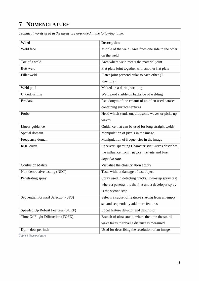
7 NOMENCLATURE
Technical words used in the thesis are described in the following table.
Word Description
Weld face Middle of the weld. Area from one side to the other
on the weld
Toe of a weld Area where weld meets the material joint
Butt weld Flat plate joint together with another flat plate
Fillet weld Plates joint perpendicular to each other (T-
structure)
Weld pool Melted area during welding
Underflushing Weld pool visible on backside of welding
Brodatz Pseudonym of the creator of an often used dataset
containing surface textures
Probe Head which sends out ultrasonic waves or picks up
waves
Linear guidance Guidance that can be used for long straight welds
Spatial domain Manipulation of pixels in the image
Frequency domain Manipulation of frequencies in the image
ROC curve Receiver Operating Characteristic Curves describes
the influence from true positive rate and true
negative rate.
Confusion Matrix Visualise the classification ability
Non-destructive testing (NDT) Tests without damage of test object
Penetrating spray Spray used in detecting cracks. Two-step spray test
where a penetrant is the first and a developer spray
is the second step.
Sequential Forward Selection (SFS) Selects a subset of features starting from an empty
set and sequentially add more features
Speeded Up Robust Features (SURF) Local feature detector and descriptor
Time Of Flight Diffraction (TOFD) Branch of ultra sound, where the time the sound
wave takes to travel a distance is measured
Dpi – dots per inch Used for describing the resolution of an image
Table 1 Nomenclature

9
8 INTRODUCTION
These days, several companies offer welding robots for every possible use. Welding robots work rapidly,
precisely, and can continue without breaks. Previously, robots were used for simple and repetitive welding
tasks, but today the robots are very refined in their movements and controls. Robots can now perform
complex welding tasks normally performed by human workers, with a speed up to 3-6 times faster than
humans [2]. Even though the robot can perform a perfect technique, the robot is not immune to errors from
the surroundings, and inspection is still required. Visual inspection and evaluation of welds is common in
commercial welding environments, but the procedure requires time and labour [3].
Visual inspection is a form of Non-Destructive Testing (NDT) where radiographic images and ultrasonic
inspections are commonly used [1]. Ultrasonic Testing (UT) requires manual interaction and interpretation,
which is time consuming and heavily dependent on the experience of skilled workers [4]. Radiography
testing requires expensive equipment and personnel who know how to read radiographic images [1]. The size
of test objects for radiographic images is limited, since it requires full access to the welding [5]. Ultrasonic
testing is more flexible in use compared to radiographic images and can be used in the field, but it also
requires a skilled person to interpret the output. Ultrasound uses a gel-based liquid between the probe and the
surface, which has to be cleaned after testing, which prolongs the time spent on the testing [6].
This project explores the quality control of welds performed with linear guidance welding – a sub-branch of
early welding robots. Even though robots perform a standardised job, flaws can occur due to technical issues,
interference of surroundings or breakdowns. A technical issue may not show up as a direct breakdown, but as
a problem with the gas supply or oxygen from surroundings, which might only affect the weld in certain
areas. The detection of defects is a time consuming and a costly affair if performed after the installation of
larger objects, i.e. scaffolding or similar constructions. Defects are important to investigate due to reduced
strength in the weld; even small defects may cause great failures and expenses.
10
8.1 BACKGROUND A dangerous term when discussing construction quality is weld joints, which is why this area is
important to research further [7]. In their work from 2002, Wang and Liao [1] state that only a
limited amount of work has been performed within the field of automatic identification of weld
defects. Even though Wang and Liao’s work was published several years ago, the area has still not
been comprehensively explored. Research papers within the area of defect recognition often relate
to the applications on digitalised images, originating from radiographic images, which makes it
possible to explore the weld in depth. Radiographic evaluation requires special cameras, high cost
equipment, and a skilled person who knows how to interpret the images and may be harmful to the
human body during prolonged exposure. Research concerning defect recognition on 2D images
from a conventional digital camera was performed by Cook et al. [3] and shows good results when
detecting shapes and other defects. The work presented by Cook et al. uses manual preparation
methods, such as a penetrating spray of the inspected area before the further processing of image,
which reduces the power of the word automatic. I am not aware of any former work that concerns
the area of defect detection based on grey scales and local patterns in 2D images obtained by an
ordinary digital camera, which is why I find this work of relevance. Similar work is performed on
digitalised radiographic images, where accepted results are presented. Combined with other works
concerning texture classification, based on grey scale features and local binary patterns, the
foundation of this thesis was created. The idea behind this thesis is to create a foundation for further
research within the area of visual inspection of weld surfaces using 2D images.

11
8.2 PROBLEM STATEMENT
The thesis attempts to find a feature extraction method and a classifier that can classify simple
surface defects in MIG welds, in order that a common quality inspection is carried out and to
eliminate the use of skilled labour in performing general inspection. Manual inspection is heavily
reliant on the person performing the investigation, which might differ from person to person [1].
Automated inspection of welds can save time and resources in the construction industry, where
welds are required to have a certain strength. Inspections performed manually are time consuming
and require skilled labour with the same standard implemented. With the help of the automation, the
skilled workers can use their expertise elsewhere and only spend time on inspection if a critical area
is detected by the model and requires further investigation. Two feature extraction methods have
been identified as promising possible solutions to the problem at hand, and will be tested on a
dataset, containing both weld defects and approved welds, created for this exact purpose. Two
classification methods are evaluated based on their ability to predict unknown data, based on
training with extracted features.

12
8.3 LIMITATION AND DELIMITATIONS
The type of welds has been limited to concern Gas Metal Arc Welding, referred to as MIG in the project.
MIG welding is used in heavy industries and in combination with welding robots [8]. Welds made with
different types of techniques have different features that might require other applications, which supports the
intention of only looking into one weld type. Different weld types requires different approaches in testing, as
is also the case with flaws and defects. This thesis only concerns defects occurring from faults in the supply
of gas. A defect related to gas supply is easy to detect during inspection and will be counted as s a valid
defect in the thesis. During the project, no tests on or with robots were performed and, based on my
experience, the influence of a welding robot would have no or very little influence on the results. Including a
welding robot in the testing would require access to a robot with a MIG welding setup, where the detection
of flaws and defects was possible. It was therefore concluded by the author and supervisors that human
fabricated weld samples would be sufficient for this type of test. The application-aim of welding robots is
based on the assumption that a welder personally checks his or her work after completion and therefore the
need for external inspection does, in theory, not exist with manual welding.
Due to no dataset being available online which could fulfil the requirements of types of images and type of
weld, a dataset was created from weld samples. The dataset was created for this specific thesis, which
resulted in a limited amount of data and types of defects. Weld images are available, but the majority of these
datasets contain digitalised radiographic images. Limited data results in small variance in the type of defects,
but the author and supervisors estimated the amount of data to be sufficient for testing. The type of samples
created for dataset makes it possible to work with classification only and not a specific detection of areas
with flaws and defects. This idea based on the setup with a camera placed just after linear guided welder
creating images for testing.

13
8.4 RELATED WORK
This chapter briefly describes published work related to the topic. This is to provide an overview of already
researched areas and to show the source of inspiration. Deeper, more explanatory details and critical
analysis regarding related work and methods are presented in the chapter, Literature Review.
Several researchers have presented promising works with feature extractors in the spatial domain. Tou et al.
[9] describe the use of Gabor features as being are at high dimensional space. A high dimensional space will
affect the classification, so to reduce the feature size, a Principal Component Analysis (PCA) is used. The
paper uses k-Nearest Neighbour (KNN) as the classifier, which requires considerable computation due to
comparison with all test samples. Other feature extractors are often used and Hassan, et al. [10] describe the
use of geometric features as shape descriptors when classifying defects in radiographic images with Artificial
Neural Network.
Hassan et al. [10] state that normal image processing tools are not useful on radiographic images and
therefore they use morphological operations to find Regions of Interest (ROI), contrast enhancement and
Canny for edge detection.
Xu et al. [11] test common algorithms used for edge detection such as Roberts, Sobel, Prewitt, Laplacian and
Canny, during real-time tracking control of welds. These tests show Canny to be the best edge detector for
their purpose. Canny’s algorithm uses Gaus function to smoothen image and high- and low thresholds to
detect edges. They find double threshold to be problematic when working with real-time detection.
Mery and Berti [12] describe the use of texture features when automatically detecting weld defects with the
use of Grey Level Co-occurrence Matrix and Gabor Filters. The authors extract features and reduce the
number of features with Sequential Forward Selection (SFS) to evaluate the performance of features and to
check for correlation before the classifier.
Common to the majority of the papers is the use of the three steps of segmentation, feature extraction and
classification. Pathak and Barooah [13] describe texture analysis based on Grey Level Co-Occurrence
Matrixes (GLCM). Sobel edge detector is applied to images, before feature extraction is performed, to
highlight corners, circles and other informant shapes. GLCM features are obtained using different angles in
the evaluation of neighbours. Collected features are tested against each other, where they state that 0̊ and 90̊
are comparable and useful for further processing. They conclude the distance between pixels evaluated and
the angle has great importance on the final result.
The use of feature extraction and classification has not only shown good results with welds, but also in wood
detection. Hittawe et al. [14] use both Local Binary Pattern (LBP) and Speeded Up Robust Features (SURF)
for defect detection in wood. LBP and SURF are tested in both isolation and combination. LBP performs
best when tested individually, but the best results are found with a combination of both methods.

14
8.5 STATE OF THE ART The following attempts to explain how this thesis separates from similar work and research. What makes this
work state of the art?
When defining features for classification, geometric shapes are often used because it seems natural for
humans to interpret based on geometric features when defining shapes. In the following, I question the use of
geometric features in computerised visual inspection, which leads to the use of methods searching for
features and patterns not recognisable to the human brain. The use of geometric features will detect features
and categorise these, but can we argue that the interpretation is different for the human brain? Methods using
non-geometric features may detect patterns that hold useful information from the image. Feature extraction
methods in the thesis will therefore only concern such methods. Feature extraction from radiographic images
is widely used in the classification of weld flaws and defects, but the feature extraction from 2D digital
images is less common. Work has been published concerning weld detection from 2D images, where the
geometric features state the appearance of the weld. I am not aware of any published work that uses 2D
images created from a regular digital camera for the classification of weld surface defects, based on features
extracted by grey level co-occurrence and local binary patterns.

15
9 METHODOLOGY
9.1 RESEARCH DESIGN
The following chapter describes the research design and the overall steps. These steps are presented to
involve the reader in some of the overall design thoughts regarding this thesis. Methods used can be found in
the chapter, Methods.
Preliminary research
Preliminary research is used in the exploration of research projects and similar topics published. The
preliminary research does not only consist of literature regarding visual inspection of welds, but also visual
inspection and texture analysis in general. Visual inspection embraces both image processing- and machine
learning theories, where surface textures can be a valuable informant. Methods are gathered from published
research papers to give an insight into methods used in other papers and the type of work that inspired this
project, based on their results and considerations behind their work.
The inspiration behind my research was based on:
1. Understanding existing literature and an overview of published research papers
2. Image processing theory
3. Machine learning theory (what type of machine learning is useful and what is the expected output)
4. Interviews with welding inspectors (experts)
5. Type of data (Types of images, dataset, flaw types etc.)
Based on interviews, research and a review of existing literature, the type of data to be used is determined.

16
Data Preparation
The overall steps for preparation of data are presented below. Choice of methods is primarily based on
methods used in published research papers.
1. Create data (images, replicate defects, defining weld quality etc.)
2. Preparing data for tests
3. Image processing for the purpose of machine learning. (What types of tool are useful and what has
created successful results in related works)
4. Feature extraction methods (extraction methods useful for this specific type of data are evaluated
based on related research papers)
5. Define the type of machine learning (Based on related work, the type of machine learning algorithms
are chosen)
6. Based on the collected data, tests are performed to find the optimal pattern recognition processes.
The image is prepared through image-processing tools and thereby processed by a machine learning
algorithm
Tests
Output from the algorithms are trained on images where known defects are present and labelled by experts.
Comparison of classification algorithms are compared and evaluated to find the best possible classifier. A
test scheme is set up to test several different combinations of inputs and classification settings.
Analysis
Evaluation and analysis of test results are discussed together with feature extraction methods. Feature
extraction methods are discussed to evaluate output regarding valuable information from weld face.
Classification results are compared to similar work, where some of the same methods are used, to evaluate
the methods.
It is discussed whether the results obtained in this thesis can contribute to further research.
17
9.2 DATA COLLECTION
The following chapter describes the methods used for data collection. A discussion regarding the methods
used is offered at the end of the chapter.
Semi-structured interviews were used in the collection of information due to the qualitative data they
provide. This method allows the interview to take another direction in comparison to a regular interview, if
the interviewees have other relevant information to the topic. The interviewer keeps track of the interview
and ensures relevant information is collected by the use of an interview guide. Semi-structured interviews are
useful if the interviewee can only be interviewed once, since this interview type gives the interviewees the
freedom to express their own thoughts, which provides reliable and comparable data [15]. The interview
guide can be found in appendix 1 - Interview guide
9.2.1 Condensed interview
This chapter highlights the important parts of the interview with Jørgen Melchior – an expert in visual
inspection of welds - FORCE Technology1 (full interview is available from link2– in Danish). The interview
started as a general discussion about the different types of visual inspection, where commonly used methods
were discussed. Jørgen Melchoir presented different types of sample, both approved and non-approved, and
the weld face appearance was discussed in relation to the dataset used in this thesis. Non-approved welds
were shown and discussed, and this discussion led to the approval of the samples made for the dataset. The
type of weld defects present in the dataset are mentioned as being seldom found during welding with linear
guidance, but not unrealistic. Different defects and flaws present in butt-welds were discussed while going
through different types of samples. Another topic was the height of the weld and geometric features in
general, but since this project works with grey scale 2D images it is not possible to read the height and the
main topic is non-geometric feature extraction.
The interview took another direction following the discussion of this project’s approach to the subject, one
concerning stainless steel welds and the finishing of the surface. Stainless steel welds create a tempering
around the weld and the colour of the tempering can evidence what type of finishing is needed to maintain a
stainless weld face. If the tempering is not removed, the welded area is not protected against rust. Based on
the discussion about colour tempering in stainless steel, colour shading around MIG welds was considered
and found less useful compared to texture analysis. Several years ago FORCE Technology tried to automate
the inspection of colour shading during welding in stainless steel, but with no luck – this topic has
encouraged further exploration and a model (later research) that can describe the colour shading. A model for
continuous colour detection was described as revolutionary by the expert at FORCE Technology. During the
discussion it was mentioned that Denmark has a thriving food industry, where high demands within stainless
steel are required and a method that could help maintain a high standard would be very attractive. During the
1 FORCE Technology - https://forcetechnology.com/da 2 https://drive.google.com/open?id=0BxMRnl6eiB0PeDE2YWs1NXFqb0E

18
interview and meeting at FORCE Technology, a visit to one of the workshops resulted in a contact with
Henrik Sørensen, who is a specialist in linear welding, which is a branch of robot welding. Henrik suggested
linear guidance, due to the use of straight welds.
9.2.2 Laboratory Tests
Laboratory testing has been the framework across all the tests. To realise the amount and quality of pictures
needed for image processing and modelling, small man-made samples had to be created. Moreover, perfect
samples, both containing non-defect samples and defect samples were needed. The sample issue was
primarily related to defect samples, which had to contain the right type of defect in the weld. Laboratory
samples were made in collaboration with blacksmith Charlotte Gilbert Jespersen at Aalborg University. In
appendix 2 - Welding settings, the settings are presented, in order that a replication can be performed.
As mentioned in Limitation and Delimitation the samples’ defects only relate to defects due to gas supply.
To create weld samples that could fulfil the requirements and potentially create the same type of defects in
all the bad samples, Samples were created in small batches of ten to twelve, all during the same day to ensure
all settings were the same.
The camera used for sampling is a normal commercial digital camera with 4608 x 3072 pixels. A
commercial digital camera was chosen based on its simplicity and to make samples easy to produce and
replicate. Images were created to only show weld faces in one direction due to the idea of a permanently
mounted camera that creates samples for inspection and to eliminate the risk of different types of reflections
from artificial lightning, see appendix 3 – Camera setup. The author and the supervisors agreed on this type
of setting, since no professional lighting equipment was available.
9.2.3 Framework
Matlab from MathWorks is used as the overall framework. There are several different other options which
can perform at the same level, but Matlab was introduced earlier during the Global Systems Design program
and therefore it seemed obvious to use. The computer used for testing is an Intel Core5 processor with 12GB
RAM. The computation power influences the processing time, and different processing time will be present
if tests need to be replicated.
Matlab offers different pre-programmed functions, of which several are used in this thesis.
Functions from Matlab are listed to provide an overview – see appendix 4 - Pre-programmed functions in
Matlab. No deeper explanation regarding functions has been given.

19
9.3 QUALITY OF RESEARCH
Here, methods used for data collection are discussed and revised to evaluate if other methods could have
provided other information.
A semi-structured interview was chosen based on the opportunity to have the interview take a different
direction, of which the interviewee may not necessarily initially be aware. As expressed in the condensed
interview, the interviewee showed interest in the topic and mentioned other areas that could be interesting for
further investigation.
A collaboration with an expert within visual inspection might have directed the data for testing in another
direction, since the interview opened a new area of interest, i.e. colour tempering, when welding in stainless
steel. However, the primary focus was visual inspection of MIG welds.
If an expert had been involved earlier in the process or throughout the tests, a broader application could have
been created. Only one interview was performed, but considerable information was collected and every
question was answered, which provided the author with all the required information at that time. A
collaboration with an expert or a company might have resulted in tests aimed for an implementation, but the
output of tests shows positive results and a strong foundation for further research within the area. The
interview was used as a validation of the thoughts behind the project and the images used in dataset.
Literature research within the area was performed in order to evaluate existing papers and the results
achieved. Papers evaluated did not only cover defects in welds, but texture classification in general, which
opens up the test and evaluates if alternative feature extraction methods could be useful for weld surfaces.
20
10 LITERATURE REVIEW
This chapter focuses on the major topic in this work – feature extraction used for texture classification.
Different works concerning classification of weld defects, but also work only interested in texture
classification, are presented and analysed in relation to other research, to then to be considered in relation
to this thesis.
Machine vision in inspection of welds is not spectacular and considerable research within the wide field has
been performed in the past. Geometric features are often used for classification, because of their ability to
visualise defects and their type [10], and when evaluating surface textures, geometric features may come to
one’s mind as one of the first interpretation options. Hassan et al. [10] tested a multi-layer multiple input
neuron model fed with geometric features extracted from radiographic images, and achieved a classification
rate above 85%. Geometric features seem an obvious choice for the human understanding and interpretation
of images, but what if the human eyes and brain were capable of looking deeper into an image and thereby
create further understanding based on, for example, grey scales? The following work concerns the surface
texture of the weld, which led me in the direction of non-geometric features to find patterns describing
surface texture. Describing textures using non-geometric features is presented in several other research
papers. In their work, Kumar et al. [16] present an approach where Grey Level Co-Occurrence Matrix
(GLCM) is used for feature extraction when detecting flaws in welds. They apply the method proposed on
digitalised radiographic images, which are converted from RGB to grey scale images. Regions of interest,
noise reduction and contrast enhancement are applied to the image before the GLCM feature extraction
method returns vectors describing the surface. In 2014, Kumar et al. [16] developed an approach to a
methodology to classify nine different types of weld flaw, whereas former classification methods were only
capable of classifying seven flaws at the maximum, and achieved an accuracy between 82,3% and 86,1%. In
2003, Merry and Berti [12] detected welding defects in radiographic images using texture features. Laplacian
edge detection is used to enhance the edges and GLCM and Gabor functions are applied on downscaled 2D
images. The features, 28 (14x2) based on [17] are obtained from GLCM and 64 from Gabor functions. To
eliminate correlated features SFS is used for evaluation, so only non-correlated features are used in the
further process. SFS feature selection states that mean of difference entropy and the mean difference variance
are the best features obtained from GLCM. A recognition rate of 84% was achieved only through the use of
features extracted by GLCM. In relation to the work performed by Kumar et al. [16] the use of edge
detection tools, which return a binary image, can be questioned when using GLCM as feature extractor,
where grey value of neighbouring pixels are evaluated. On the other hand, the return of a binary image might
become useful if used for the detection of welds and the shape of these, but when dealing with texture
features it can be questioned if loss of information is too high.
Merry and Berti [12] combined all features extracted from two methods (GLCM and Gabor Functions), and
saw that only features extracted by Gabor functions were selected during feature reduction with SFS. This

21
creates doubt as to whether GLCM feature extraction is suitable for further testing. In 2007, Tou et al. [9]
tested GLCM and Gabor functions separately and in combination, where GLCM achieved a recognition rate
of 84% and Gabor functions only achieved 80%, which again questions the comparison by Merry and Berti
[12]. Tou et al. [9] used Brodatz’s3 texture dataset, a dataset containing wood-, stone- and rock types for
testing and applied commonly used statistical features (Energy, Entropy, Contrast and Homogeneity)
calculated from GLCM with grey levels between 8 and 256 and the spatial distance between one and five
pixels. The best result is achieved with 64 grey levels and a spatial distance of two. Gabor functions
produced over 6000 features and downsampling was executed with the use of PCA. The best result is
achieved when using six features, since the decision rate is decreased when adding or removing features.
Extracting 6000 features may seem overwhelming, and when reduced to six features in the end, due to good
test results, I find it appropriate to continue with GLCM instead of Gabor Functions.
Tou et al. [9] experienced a decreasing decision rate when applying more than six features to the classifier. A
decreasing decision rate shows the direct influence of the feature space which, in this case, is large, and has a
negative influence. Another issue with extracting large numbers of features is the need of further
decomposing before classification, which requires computation time and extra resources. Depending on the
type of data used in other research, different preparation methods and GLCM settings are used. Mohanaiah et
al. [18] state that image size plays a role in the feature output, where the value of extracted features increases
proportionally as the image size increases. Their tests show 128x128 as the optimal image size for their data,
where the loss of information is at a minimum. The increasing of valuable features corresponding to
increasing image size seems obvious, but optimal image size might differ depending on the type of images
and optimal different image resolutions and should be tested individually.
Silva et al. [19] concluded in their 2004 work that the quality of features is more important to the result of
the classifier than the quantity. Quality features are weighted above feature quantities in this work, due to the
risk of correlation and declining accuracy when using more than six features [9]. Based on the results from
Tou et al. [9], a limited number of features, four features with GLCM, are extracted for further processing
during this work. Depending on image size, the optimal neighbourhood offset can be discussed and, based on
published research papers, an estimation of proper offset can be made. Another setting is the direction to the
evaluated neighbour (0̊, 45̊, 90̊ & 135̊). Mohanaiah et al. [18] create the Grey Level Co-Occurrence Matrix
with an offset of one pixel to the neighbour and state that a larger offset can be used if the window is
sufficiently large. The direction of the evaluated neighbour is unspecified, which I conclude to be because
they use the predefined direction (neighbour to the east or 0̊). Tou et al. [9] performed experiments with all
four directions to find the best grey level and spatial distance to the neighbour. They performed seven
experiments with grey levels between 8 and 256 and the spatial distance (offset) between one and five, to
conclude the best accuracy was found with 64 grey levels and a distance of two. Tests performed4 on the data
3 See Appendix 5 - Brodatz’s Dataset for example. 4 https://drive.google.com/open?id=0BxMRnl6eiB0PYnlqeHlFbmpLM0E
22
used for this thesis show identical values when evaluating the neighbour at 0 ̊ and 90̊, which is why the use of
both directions are not considered.
Local Binary Pattern (LBP) has, since its foundation by Ojala et al. [20] , received considerable attention and
has been used in many applications. However, the conventional method proposed in 1996 faces some
limitations which might influence the quality of features, due to small spatial region, noise sensitivity and
global textural information [21]. Guo et al. [22] proposed an extension of LBP, named Completed LBP
(CLBP), where a comparison of the original and simple LBP and the extended CLBP is made based on
feature extraction from two different datasets. Guo et al. [22] explain how the simple LBP extracts
reasonable texture features, though it only uses signs and is not looking at magnitude as a descriptor. Even
though reasonable features can be found by the simple LBP, there are some pitfalls which need to be
considered, e.g. incorrect matches of local structures. If two different vectors with large difference between
the values, have the same sign vector, they will appear as similar local structures, but in fact, they are very
different in structure. The risk of incorrect match questions the use of the simple LBP as the only feature
extraction method, but due to the type of images in dataset used for this work, the risk of incorrect matches is
estimated to be limited. The extension of the original LBP operator works with the term uniform patterns. A
pattern is called uniform when it has less than two 0-1 (or opposite) transitions in the binary circular
presentation [22]. Ojala, et, al. [23] state that uniform patterns provide the majority (90%) of patterns in a
3x3 texture pattern. Uniform patterns are influenced the fact that some kind of binary patterns occur more
often in textures than others and the ability to reduce the size of the feature vector from 256 to 59. The work
performed by Guo et al. [22] finds that texture classification using sign features achieves better results
compared to classification using magnitude features. What is worth mentioning is the enhancement of
classification results if both sign- and magnitude features are combined [22]. Due to an idea of a simple
feature extraction method, the higher accuracy from the extended version has been estimated to have little
influence on dataset used in this work. LBP extracts more features than GLCM, which means 10 or 59
features are extracted due to the change between uniform LBP features or uninorm rotationally invariant
LBP features.
The preparation of images for feature extraction is performed in different ways, depending on type of data
and what the authors find to be a proper preparation. Gudla et al. [24] propose a method where a modified
neighbourhood in LBP, with non-symmetrical neighbours are considered in images normalised to a
resolution of 200 x 200 and further divided into non-overlapping blocks of 25 x 25. When considering non-
symmetrical neighbours the need for interpolation (to place the pixel in the centre of the neighbourhood) is
eliminated. In traditional LBP, the number of neighbours increases with increase of radius, which results in a
unique description of the neighbourhood, but the increased radius eliminates the information from pixels
very close to the reference pixel [24]. Results from LBP with a modified neighbourhood compared with
results from the traditional LBP with symmetrical neighbours show slightly better accuracy from the
modified neighbourhood on their data concerning gender recognition based on textures in faces. This method

23
of non-symmetrical neighbours provides the opportunity to look at both the local and global neighbourhood
without loss of information. It can be discussed if LBP with modified neighbourhood would create
significantly better results compared to the simple uniform LBP method based exclusively on one image
dataset containing faces. It is assumed that global information from images containing welds, where weld
face is placed in the vertical centreline of images, is less important compared to local information.
To evaluate extracted features, a classifier is used and the accuracy is the measured value. This project does
not concern only one specific classifier, but two well-known classifiers, Support Vector Machine (SVM) and
K-Nearest Neighbour (KNN), with promising results will be tested with extracted features. Support Vector
Machine (SVM) presented by Cortes, et.al [25] is a well-known classifier and often used for texture
classification. SVM uses a limited amount of sampling data in the training model and obtain a more or less
fixed hyperplane for classification [26]. Meng et al. [26] state the use of a relatively fixed hyperplane could
have a serious influence if working with dynamic failures. I can confirm that it makes little sense to use
similar hyperplanes to different types of failures, as their features will probably appear different. In this case,
images in the dataset will be of a common quality and only one type of defect has to be classified, which
leads to the simple SVM as a useful classifier. Murosaki et al. [27] used SVM to detect grey areas, as a result
of overheating during welding, in fuel pumps with features, such as energy, contrast, entropy and
homogeneity and achieved good results.
Ahmed et al. [28] tested the performance of textural features obtained from the Brodatz dataset with KNN
and achieved good results. KNN calculates the distance from each training sample to the test sample and
chooses the closest one [29]. The size of k (pixels to the nearest neighbour) varies and no exact value can be
pointed out as the best. K-value may differ from the type of dataset, where a small k-value may be sensitive
to noise, where a large k-value may include too many points from other classes [29].
Further explanation of the settings used during testing is described in Test Settings.

24
11 TECHNICAL INTRODUCTION
The following will introduce the term of welding robots, along with different welding techniques and weld
types. This introduction is to give insight into why some methods are chosen above others. After a general
technical introduction, methods for testing of welds are briefly introduced.
11.1.1 Welding Robots
Welding robots can be defined as positioning controlled devices that can perform a continuous movement
[30]. Welding robots are one of the most common worldwide applications, and even smaller production
facilities have started to take advantage of robots. The robot is controlled by the programming and is not
capable of making judgement or corrections itself, which means there is a demand for inspection of the weld
[30]. In the manufacturing of straight welds, linear seam welding machines are part of the early welding
robots, but are still used where the fabrication dimension requires long weld seams. Linear seam welding
machines can be referred to as fixed automation, where the equipment and the configurations are fixed.
Programming of linear seam welding machines is individual for each material, thickness and design, which
decreases processing time, but also decreases production flexibility and product variety. Robots and welding
machines can be adapted to perform all available welding techniques, which makes them useful in many
applications.
11.1.2 Welding Techniques
Several types of welding are used in the industry and the following introduces the three most common. Gas
Metal Arc Welding (GMAW) also described as MIG (Metal Inert Gas) or MAG (Metal Active Gas), which
uses a continuous fed wire electrode, which, besides being the electrode, also adds joint material to the weld
pool. During welding, the electrode and weld pool are protected from the surrounding air by a shielding inert
gas (or active gas if MAG) to avoid oxygen mixing in the weld pool. GMAW is a common process that is
widely used for industrial welding applications. Gas Tungsten Arc Gas Welding (GTAW) or TIG (Tungsten
Inert Gas) is a type of welding that requires more expertise compared to GMAW, because the electrode and
joint material are separated and controlled individually. GTAW is known for producing high-quality work
with a superior finish. Shielded Metal Arc Welding (SMAW) also known as Arc Welding, is the most basic
of welding types. Arc welding is used in construction, manufacturing and repairs and is suited for heavier
material thickness. Electrode, joint material and shield from surrounding air are provided all in one. A solid
powder forms the covering shield and protects the weld pool during burning. [8], [31]
25
11.1.3 Weld types
Weld types can be divided in two overall groups: Groove weld and fillet-type weld. Groove weld fills in the
groove between the pieces joined together, while fillet weld fills in the area on the outside of the pieces
joined together [32] [33]. Groove weld is also known as Butt Joints, while Fillet welds encompasses Corner
Joint, Edge Joint, Lap Joint and Tee Joint. Common to all weld types is the structure, which should have a
uniform shape without defects [7].
A butt weld is where two pieces are joined together in the same plane. A corner joint is where two pieces
form either an L-shape or an A-shape to make a corner. An edge joint is where the pieces are placed up
against each other and the edges welded together. A lap joint is where two pieces are placed on top of each
other with an overlap where the weld is placed. A tee joint is, as the name suggests, a weld where two pieces
form a T-shape and the weld can be placed on both sides of the tee [33]. A butt weld is widely used in simple
designs and fabrication of pipe systems [32]. Finally, fillet welds are estimated to be the most used type of
welding in fabrication. The use of fillet welding does not require any preparation of the edges, which makes
this type of weld cheaper and quicker [32]. Despite many different weld joints being used in manufacturing,
tests are only applied on images showing butt joints on sheet metal with a thickness of two millimetres.
11.2 NON-DESTRUCTIVE TESTING
The following introduces some of the methods used for Non-Destructive Testing (NDT). NDT is used in
manufacturing control and embraces several different techniques, including Visual Inspection, Radiographic
Testing and Ultrasonic Testing [34]. NDT techniques are used to detect defects and flaws which have
occurred during manufacturing or caused by stressful environments, without penetration of the surface [34].
11.2.1 Visual Inspection of Welds
Visual inspection encompasses different specifications provided by International Organization for
Standardization (ISO), of the overall procedure of the inspection. The weld must be inspected to check that
slag has been removed to avoid imperfections [35]. Butt welds and fillet welds are examined to ensure joints
merge smoothly with the main components without underflushing, convexity or concavity. Placement of the
seam, weld profile and surface patterns are examined for irregularities according to the manufacturer’s
specifications [35]. Imperfections such as cracks and porosity are examined with the use of optical aids to
ease the inspection [35]. To ensure that the respective work is carried out using the same criteria,
International Organization for Standardization (ISO) has set up standards which companies can choose to
follow and thereby achieve the ISO standard. ISO 5817 is a standard concerning quality levels for
imperfections in fusion-welded joints in steel, nickel, titanium and alloys. Quality levels are divided into
three categories: B, C & D (B represents the highest level) [36]. ISO 6520 defines types of flaws and defects
found in fillet- and butt welds. Some types of flaw are visible at weld face while others are hidden under the
surface and require test equipment that is able to examine in depth, i.e. radiographic images or ultrasound.
Some of the flaws and defects stated in the standard are cracks, gas pores, porosity, craters, lack of fusions,

26
penetrations, grooves, misalignments and burn through [37]. ISO 6520 concerns, among others, cracks, holes
and porosity. The different types of flaw and defect can, in some instances, e.g. in quality level D, be
accepted if not exceeding predefined limits, but in general flaws should be avoided.
11.2.2 Radiographic Testing
NDT with radiographic images requires access to both sides of the weld or the object inspected because the
film must be placed at the right angle to catch the radiation. The films must overlap to ensure the complete
area is covered [5]. Two types of radiographic sensitivities are used in the examination: Class A – Basic
Techniques and Class B – Improved Techniques. Class A is normally used and Class B is used if Class A is
found to be insufficient. Different techniques of how to place the film are used based on the type of weld
examined to ensure the same procedure is used [5]. If the film is placed incorrectly, the defects will not occur
correctly and might be overlooked.
11.2.3 Ultrasonic Testing
Ultrasonic is a NDT method that uses an ultrasonic beam, which is reflected from the opposite side and
captured by a transducer. The structure of the wave is inspected by a qualified person who can interpret
defects from the shape of the waves [6]. Time of Flight Diffraction (TOFD) is a branch of ultrasonic testing
used in metallurgy. Two probes are placed on opposite sides of the weld, of which one is the transmitter and
the other is the receiver [38]. Waves are sent through the weld and if, for example, a crack is present, the
time the wave is traveling is longer and by measuring the time, size and state of defect can be monitored
[38].

27
12 METHODS
The following chapter describes the theoretical part of the methods. Common to the papers used in this work,
three overall steps are performed - segmentation, feature extraction and classification. These steps are
described in the following to give insight in their role and why they are used. Appendix 4 - Pre-programmed
functions in Matlab gives a list of tools and functions found in Matlab, which have been used during tests.
12.1 IMAGE PREPARATION
When working with automated classification, several challenges are faced, for instance high-clutter
background, noise and variations from scaling, rotation or similar [39]. To reduce computation time and
enhance the work of the feature extraction method, images in the dataset are cropped to remove excess areas
with no relevant information. Edge detection is also widely used in data preparation for feature extraction
and several different ones are available, e.g. Canny and Sobel. Edges in images are represented by intensity
in contrast and these changes in contrasts are used by Canny and Sobel to detect edges, which are two
frequently used methods. Common to both edge detectors is the use of convolution kernels and the return of
an output of either background or edge, where the edge will be white and the background black [40]. Sobel
performs a spatial gradient measure and emphasises high frequency areas, which correspond to edges. Canny
smooths an image with a Gaussian filter and then applies the same technique as Sobel, but with the
difference that Canny is not limited to a 3x3 mask, but has adjustable masks [40]. Often seen in image
preparation of datasets is normalisation, for instance, image dimensions, which is used in Brodatz’s texture
dataset [20], [23], [41], [42]. Normalisation ensures that the data input shares a common standard (grey scale,
dimensions etc.), which is used in the settings for feature extraction.
12.2 FEATURE EXTRACTION
Features are data and derived values that are informative regarding a shape in an image.
Feature extraction is a common term for methods used for construction of features from a dataset. It is
desirable to reduce the number of features in a dataset, to lower the resources used for computation and to
minimise the risk of overfitting and redundancy of features. Wang and Liao [1] suggest the best texture
descriptors to be small numbers of features with high discriminating power.
Geometric features are used to describe image features, but normally simple geometric features can only
describe shapes with large differences, in some cases filters are used to eliminate, for example, false hits
[43]. Frequency and grey scale are, among others, also used in texture description. Describing texture and
extracting features are performed in different domains, Spatial and Frequency, depending on the method
used. Spatial domain concerns techniques based on the manipulation of pixels in the image and Frequency
Domain concerns the frequencies in the image. There are several different feature extraction methods
28
described in Related Work that are useful for texture classification, but the following will only concern
GLCM and LBPs, which both work in the spatial domain of the image.
12.2.1 Grey Level Co-occurrence Matrix
Grey Level Co-occurrence Matrix (GLCM) is a statistical method for analysing the spatial distribution of
grey level values in images and was introduced by Haralick et al. [17]. Spatial distribution of grey level
values is a texture-defining quality feature and is useful for feature extraction [13]. This method evaluates the
representation of the frequency occurrence between two grey levels within a given area [44]. GLCM uses
second-order texture calculations when considering relationship between neighbouring pixels in an image
and creates a square matrix [13]. The matrix reveals how often a specific relationship between neighbouring
pixels occurs. The relationship between neighbours can be obtained from different angles (0̊, 45̊, 90̊ & 135̊).
However, normally 0 ̊, neighbour to the east, is the direction used [13]. Working with statistical texture
analysis, features describing the image are computed from statistical calculation obtained from specified
positions relative to each other [18]. Fourteen different statistic tasks can be applied to the matrix, though
Contrast, correlation, energy and homogeneity are the four most commonly used [45]. These four statistical
features have a high discrimination accuracy, reduced computation time and results show high efficiency
when used for real-time pattern recognition [18]. Grey scale images normally have 256 grey levels and by
the use of all levels, the image will be clearer, but the computation time will also be increased. When
decreasing the grey level, some features decrease and some may increase, and grey level can be estimated
based on the statistical features used. Contrast – Measures the intensity contrast between a pixel and the
specified neighbour, where zero (0) is the contrast value for a constant image. Correlation – returns a value
that describes the correlation between a pixel to a specified neighbour. The range is between -1 and 1,
describing either perfectly positive- or negative correlation. Energy – returns the sum of squared elements in
the Grey Level Co-Occurrence Matrix and describes the textural uniformity in the image, where a value of 1
is for a constant image. Homogeneity – describes the closeness of the elements distribution in the GLCM to
the diagonal. The highest value is when most of the occurrences are concentrated near the diagonal [46],
[47].
29
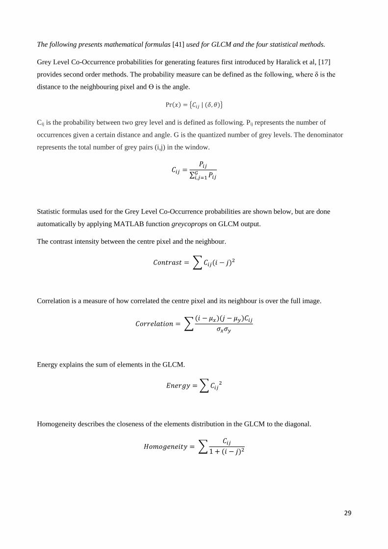
The following presents mathematical formulas [41] used for GLCM and the four statistical methods.
Grey Level Co-Occurrence probabilities for generating features first introduced by Haralick et al, [17]
provides second order methods. The probability measure can be defined as the following, where δ is the
distance to the neighbouring pixel and ϴ is the angle.
Pr(𝑥) = {𝐶𝑖𝑗 | (𝛿, 𝜃)}
Cij is the probability between two grey level and is defined as following. Pij represents the number of
occurrences given a certain distance and angle. G is the quantized number of grey levels. The denominator
represents the total number of grey pairs (i,j) in the window.
𝐶𝑖𝑗 =𝑃𝑖𝑗
∑ 𝑃𝑖𝑗𝐺𝑖,𝑗=1
Statistic formulas used for the Grey Level Co-Occurrence probabilities are shown below, but are done
automatically by applying MATLAB function greycoprops on GLCM output.
The contrast intensity between the centre pixel and the neighbour.
𝐶𝑜𝑛𝑡𝑟𝑎𝑠𝑡 = ∑ 𝐶𝑖𝑗(𝑖 − 𝑗)2
Correlation is a measure of how correlated the centre pixel and its neighbour is over the full image.
𝐶𝑜𝑟𝑟𝑒𝑙𝑎𝑡𝑖𝑜𝑛 = ∑(𝑖 − 𝜇𝑥)(𝑗 − 𝜇𝑦)𝐶𝑖𝑗
𝜎𝑥𝜎𝑦
Energy explains the sum of elements in the GLCM.
𝐸𝑛𝑒𝑟𝑔𝑦 = ∑ 𝐶𝑖𝑗2
Homogeneity describes the closeness of the elements distribution in the GLCM to the diagonal.
𝐻𝑜𝑚𝑜𝑔𝑒𝑛𝑒𝑖𝑡𝑦 = ∑𝐶𝑖𝑗
1 + (𝑖 − 𝑗)2
30
12.2.2 Local Binary Pattern
Local features refer to the pattern found in an image, which can be edges, patches in the image or similar.
What the feature represents is not necessarily relevant, what is relevant is if the features describe something
that distinguishes itself from the surroundings [48]. When working with local features, image segmentation
is not required, which makes it widely used for classification. Local features are robust regarding rotation,
clutter or other changes in viewing conditions [48]. To obtain a good local feature, the surrounding
neighbourhood of the feature centre should be sufficiently varied to allow for a proper comparison of
features. Ojala et al. [20] present the first Local Binary Pattern (LBP) as a method for texture classification,
where the overall idea behind was a descriptor that uses two complementary measures, such as grey scale
contrast and local patterns. LBP is a general definition of a texture in a local neighbourhood and provides a
binary code that describes texture pattern by using the value of the centre pixel as threshold. The local binary
code explaining the neighbourhood is produced by multiplying the threshold with a given weight to the
corresponding pixel and thereafter summing up. LBP texture description was originally obtained from a 3x3
window by using the grey value in the neighbouring pixel as a threshold. In [23] Ojala et al. presented LBP
as a method that was able to work with neighbourhoods of different size and invariant to rotation of inputs.
LBP defines the texture of a local neighbourhood in a monochrome image. Circular symmetrical neighbours
form a circle around the centre pixel to create a local neighbourhood. If the value of the neighbour is not
placed in the middle of the pixel, interpolation is used for estimation. The grey value of the neighbouring
pixel is used as a threshold to the grey value in the centre pixel, multiplication of the threshold with the given
value for the pixel (grey value), and summing up the result.
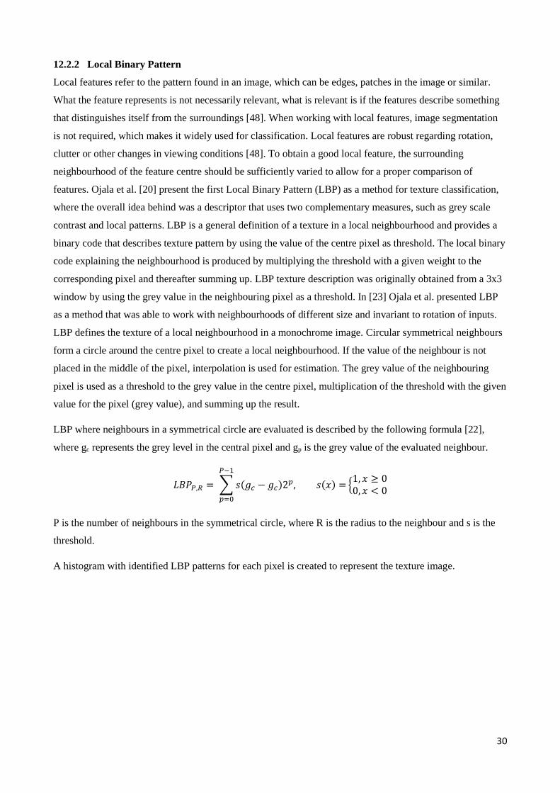
LBP where neighbours in a symmetrical circle are evaluated is described by the following formula [22],
where gc represents the grey level in the central pixel and gp is the grey value of the evaluated neighbour.
𝐿𝐵𝑃𝑃,𝑅 = ∑ 𝑠(𝑔𝑐 − 𝑔𝑐)2𝑝, 𝑠(𝑥) =
𝑃−1
𝑝=0
{1, 𝑥 ≥ 00, 𝑥 < 0
P is the number of neighbours in the symmetrical circle, where R is the radius to the neighbour and s is the
threshold.
A histogram with identified LBP patterns for each pixel is created to represent the texture image.
31
Ojala et al.[23] introduced the use of uniform patterns in 2002, based on results showing the majority of the
patterns in a 3x3 block was uniform, which in some cases it was over 90%.
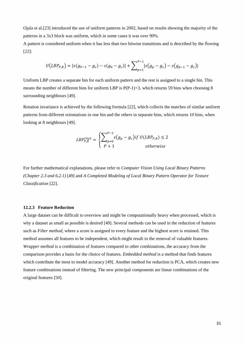
A pattern is considered uniform when it has less than two bitwise transitions and is described by the flowing
[22]:
𝑈(𝐿𝐵𝑃𝑃,𝑅) = |𝑠(𝑔𝑃−1 − 𝑔𝑐) − 𝑠(𝑔0 − 𝑔𝑐)| + ∑ |𝑠(𝑔𝑝 − 𝑔𝑐) − 𝑠(𝑔𝑝−1 − 𝑔𝑐)|𝑃−1
𝑝=1
Uniform LBP creates a separate bin for each uniform pattern and the rest is assigned to a single bin. This
means the number of different bins for uniform LBP is P(P-1)+3, which returns 59 bins when choosing 8
surrounding neighbours [49].
Rotation invariance is achieved by the following formula [22], which collects the matches of similar uniform
patterns from different orientations in one bin and the others in separate bins, which returns 10 bins, when
looking at 8 neighbours [49].
𝐿𝐵𝑃𝑃,𝑅𝑟𝑖𝑢2 = {
∑ 𝑠(𝑔𝑝 − 𝑔𝑐)𝑖𝑓 𝑈(𝐿𝐵𝑃𝑃,𝑅) ≤ 2𝑃−1
𝑝=0
𝑃 + 1 𝑜𝑡ℎ𝑒𝑟𝑤𝑖𝑠𝑒
For further mathematical explanations, please refer to Computer Vision Using Local Binary Patterns
(Chapter 2.3 and 6.2.1) [49] and A Completed Modeling of Local Binary Pattern Operator for Texture
Classification [22].
12.2.3 Feature Reduction
A large dataset can be difficult to overview and might be computationally heavy when processed, which is
why a dataset as small as possible is desired [49]. Several methods can be used in the reduction of features
such as Filter method, where a score is assigned to every feature and the highest score is retained. This
method assumes all features to be independent, which might result in the removal of valuable features.
Wrapper method is a combination of features compared to other combinations, the accuracy from the
comparison provides a basis for the choice of features. Embedded method is a method that finds features
which contribute the most to model accuracy [49]. Another method for reduction is PCA, which creates new
feature combinations instead of filtering. The new principal components are linear combinations of the
original features [50].

32
12.3 MACHINE LEARNING
The following will briefly introduce Machine Learning to provide a basic understanding of the term. Two
types of machine learning tools are presented as some of them are used in this thesis. The types of classifier
represent two categories– Eager Learners and Lazy Learners.
Machine learning is a part of Artificial Intelligence and explores the construction of algorithms that can learn
from data [51]. Machine Learning provides a computer with the opportunity to lean without programming,
by training on known data [52]. Within machine learning two sub groups encompassing supervised- and
unsupervised learning are used. Supervised learning operates under supervision due to known target values.
During training, the outcome is provided – in this case “good weld” or “bad weld”. A sub-branch in
Supervised Learning is Classification, where the outcome of the classification is referred to as class and, to
test the success, the classifier is tested on data with known class, but not known to the classifier. The success
is normally measured on the error rate [52]. The output of the final algorithm is a decision boundary
separating classes. Unsupervised Learning concerns, as the name suggests, unsupervised learning, where
target values are unknown. During Supervised Learning, the machine is introduced to the different classes,
where unsupervised learning will learn from data provided and from that describe the structure of unlabelled
data. An evaluation of the accuracy is not possible and to test the algorithm, a manual evaluation based on
historic data where output is known can be performed [52]. This requires the ability of manual interpretation
of the historic data.
33
12.3.1 Classification methods
Classification is a process to find a model that can describe and distinguish between classes in a pool of data.
The idea behind is to be able to predict or classify unknown data, based on the information from data used
for training [53]. Patterns in data needs to be presented to the classifier, thus must the data be explored and
informative features extracted. The first step in a classifier is training, where the classifier is build based on
predetermined classes. Patterns describing each class are learned and used in the prediction of new data.
Classification accuracy is determined by testing how well the model classifies unknown data. Two well-
known classifiers, Support Vector Machine and k-Nearest Neighbour, which have presented good
classification results [27], [26], [7], [54] are tested. Support Vector Machine (SVM) is categorised as an
eager learner, where the method based on a given training set construct a generalization model, which is
used when testing unknown data [53]. The SVM transforms data into a higher dimension, where separation
of data is achieved by a hyperplane. The hyperplane can both be linear or non-linear depending on method
used and the distance from the nearest data point on both sides of the hyperplane describes the best suitable
for the data [53]. SVM is known to be resilient to overfitting because the boundary only depends on a few
points. A few points describing the boundary means it will not result in overfitting of data, since it only
depends on few support vectors [55].
K-Nearest Neighbour (KNN) is categorised as a lazy learner, which is the opposite of the eager learner.
KNN searches the pattern space to look for the neighbour closest to the unknown data presented to the
classifier. An eager learner constructs a model for classification with input from training data and apply
algorithm on test data. A lazy learner does not build a model explicitly and the making of a lazy learner
model is cheap, but when it comes to the classification part that is where it becomes more time consuming. A
lazy learner like KNN will have to calculate every distance between the unknown test object and the labelled
objects in the training data, which can be computational heavy when working with large dataset [56]. KNN
implements rote learning, where classification is based on a search for exact matches or close to exact match.
It learns the patterns from the training data and classifies test data based on the search for matches [57].
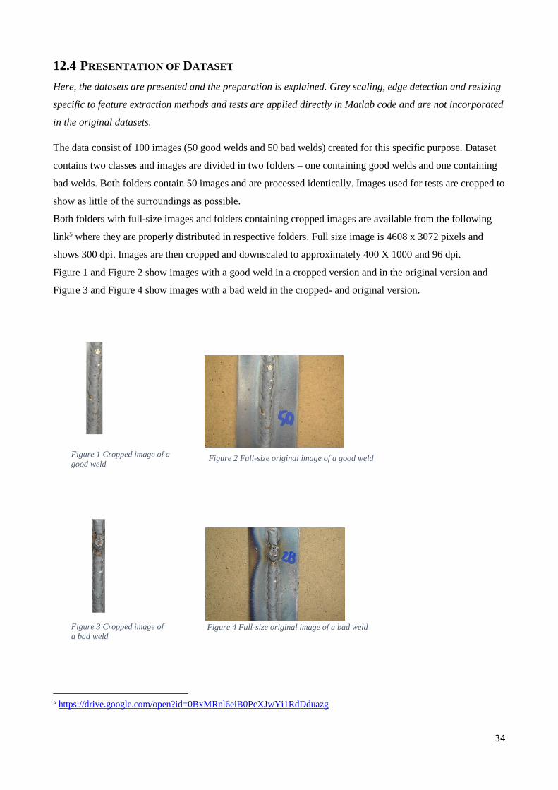
34
12.4 PRESENTATION OF DATASET
Here, the datasets are presented and the preparation is explained. Grey scaling, edge detection and resizing
specific to feature extraction methods and tests are applied directly in Matlab code and are not incorporated
in the original datasets.
The data consist of 100 images (50 good welds and 50 bad welds) created for this specific purpose. Dataset
contains two classes and images are divided in two folders – one containing good welds and one containing
bad welds. Both folders contain 50 images and are processed identically. Images used for tests are cropped to
show as little of the surroundings as possible.
Both folders with full-size images and folders containing cropped images are available from the following
link5 where they are properly distributed in respective folders. Full size image is 4608 x 3072 pixels and
shows 300 dpi. Images are then cropped and downscaled to approximately 400 X 1000 and 96 dpi.
Figure 1 and Figure 2 show images with a good weld in a cropped version and in the original version and
Figure 3 and Figure 4 show images with a bad weld in the cropped- and original version.
Figure 2 Full-size original image of a good weld
Figure 4 Full-size original image of a bad weld
5 https://drive.google.com/open?id=0BxMRnl6eiB0PcXJwYi1RdDduazg
Figure 1 Cropped image of a
good weld
Figure 3 Cropped image of
a bad weld
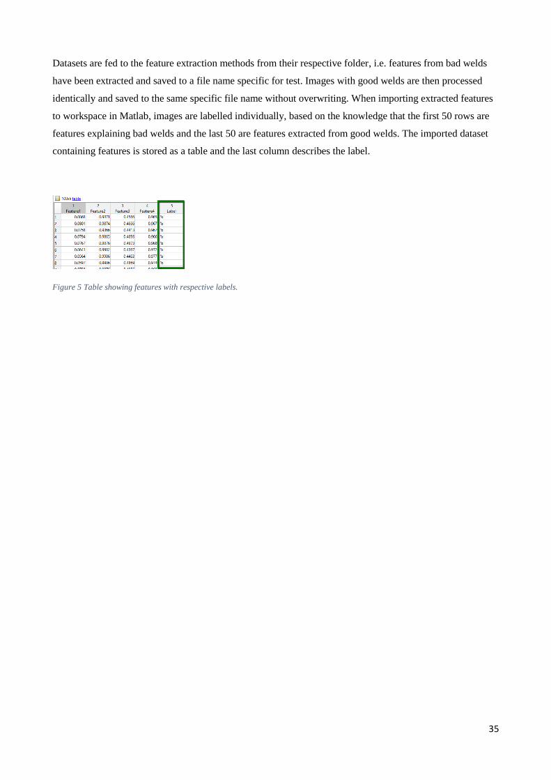
35
Datasets are fed to the feature extraction methods from their respective folder, i.e. features from bad welds
have been extracted and saved to a file name specific for test. Images with good welds are then processed
identically and saved to the same specific file name without overwriting. When importing extracted features
to workspace in Matlab, images are labelled individually, based on the knowledge that the first 50 rows are
features explaining bad welds and the last 50 are features extracted from good welds. The imported dataset
containing features is stored as a table and the last column describes the label.
Figure 5 Table showing features with respective labels.
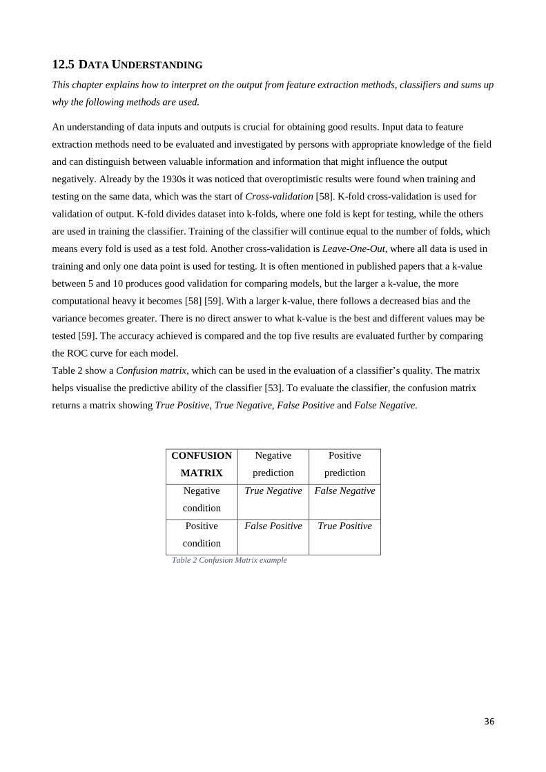
36
12.5 DATA UNDERSTANDING
This chapter explains how to interpret on the output from feature extraction methods, classifiers and sums up
why the following methods are used.
An understanding of data inputs and outputs is crucial for obtaining good results. Input data to feature
extraction methods need to be evaluated and investigated by persons with appropriate knowledge of the field
and can distinguish between valuable information and information that might influence the output
negatively. Already by the 1930s it was noticed that overoptimistic results were found when training and
testing on the same data, which was the start of Cross-validation [58]. K-fold cross-validation is used for
validation of output. K-fold divides dataset into k-folds, where one fold is kept for testing, while the others
are used in training the classifier. Training of the classifier will continue equal to the number of folds, which
means every fold is used as a test fold. Another cross-validation is Leave-One-Out, where all data is used in
training and only one data point is used for testing. It is often mentioned in published papers that a k-value
between 5 and 10 produces good validation for comparing models, but the larger a k-value, the more
computational heavy it becomes [58] [59]. With a larger k-value, there follows a decreased bias and the
variance becomes greater. There is no direct answer to what k-value is the best and different values may be
tested [59]. The accuracy achieved is compared and the top five results are evaluated further by comparing
the ROC curve for each model.
Table 2 show a Confusion matrix, which can be used in the evaluation of a classifier’s quality. The matrix
helps visualise the predictive ability of the classifier [53]. To evaluate the classifier, the confusion matrix
returns a matrix showing True Positive, True Negative, False Positive and False Negative.
CONFUSION
MATRIX
Negative
prediction
Positive
prediction
Negative
condition
True Negative
False Negative
Positive
condition
False Positive True Positive
Table 2 Confusion Matrix example
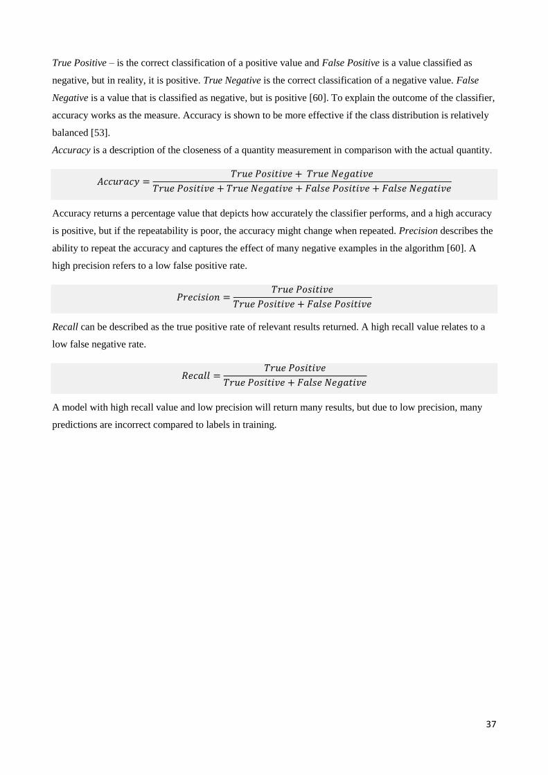
37
True Positive – is the correct classification of a positive value and False Positive is a value classified as
negative, but in reality, it is positive. True Negative is the correct classification of a negative value. False
Negative is a value that is classified as negative, but is positive [60]. To explain the outcome of the classifier,
accuracy works as the measure. Accuracy is shown to be more effective if the class distribution is relatively
balanced [53].
Accuracy is a description of the closeness of a quantity measurement in comparison with the actual quantity.
𝐴𝑐𝑐𝑢𝑟𝑎𝑐𝑦 =𝑇𝑟𝑢𝑒 𝑃𝑜𝑠𝑖𝑡𝑖𝑣𝑒 + 𝑇𝑟𝑢𝑒 𝑁𝑒𝑔𝑎𝑡𝑖𝑣𝑒
𝑇𝑟𝑢𝑒 𝑃𝑜𝑠𝑖𝑡𝑖𝑣𝑒 + 𝑇𝑟𝑢𝑒 𝑁𝑒𝑔𝑎𝑡𝑖𝑣𝑒 + 𝐹𝑎𝑙𝑠𝑒 𝑃𝑜𝑠𝑖𝑡𝑖𝑣𝑒 + 𝐹𝑎𝑙𝑠𝑒 𝑁𝑒𝑔𝑎𝑡𝑖𝑣𝑒
Accuracy returns a percentage value that depicts how accurately the classifier performs, and a high accuracy
is positive, but if the repeatability is poor, the accuracy might change when repeated. Precision describes the
ability to repeat the accuracy and captures the effect of many negative examples in the algorithm [60]. A
high precision refers to a low false positive rate.
𝑃𝑟𝑒𝑐𝑖𝑠𝑖𝑜𝑛 =𝑇𝑟𝑢𝑒 𝑃𝑜𝑠𝑖𝑡𝑖𝑣𝑒
𝑇𝑟𝑢𝑒 𝑃𝑜𝑠𝑖𝑡𝑖𝑣𝑒 + 𝐹𝑎𝑙𝑠𝑒 𝑃𝑜𝑠𝑖𝑡𝑖𝑣𝑒
Recall can be described as the true positive rate of relevant results returned. A high recall value relates to a
low false negative rate.
𝑅𝑒𝑐𝑎𝑙𝑙 =𝑇𝑟𝑢𝑒 𝑃𝑜𝑠𝑖𝑡𝑖𝑣𝑒
𝑇𝑟𝑢𝑒 𝑃𝑜𝑠𝑖𝑡𝑖𝑣𝑒 + 𝐹𝑎𝑙𝑠𝑒 𝑁𝑒𝑔𝑎𝑡𝑖𝑣𝑒
A model with high recall value and low precision will return many results, but due to low precision, many
predictions are incorrect compared to labels in training.
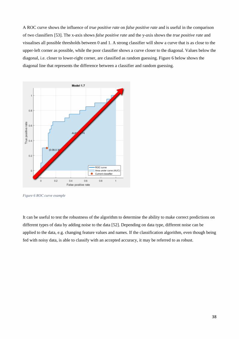
38
A ROC curve shows the influence of true positive rate on false positive rate and is useful in the comparison
of two classifiers [53]. The x-axis shows false positive rate and the y-axis shows the true positive rate and
visualises all possible thresholds between 0 and 1. A strong classifier will show a curve that is as close to the
upper-left corner as possible, while the poor classifier shows a curve closer to the diagonal. Values below the
diagonal, i.e. closer to lower-right corner, are classified as random guessing. Figure 6 below shows the
diagonal line that represents the difference between a classifier and random guessing.
Figure 6 ROC curve example
It can be useful to test the robustness of the algorithm to determine the ability to make correct predictions on
different types of data by adding noise to the data [52]. Depending on data type, different noise can be
applied to the data, e.g. changing feature values and names. If the classification algorithm, even though being
fed with noisy data, is able to classify with an accepted accuracy, it may be referred to as robust.

39
12.6 DATA PREPARATION
The following attempts to explain the preparation of data and the importance of this. Image processing tools
are presented, where a part of data preparation is image labelling, which is explained in context to the
classifier.
12.6.1 Image Processing
GLCM and LBPs both work with binary images, which means all images are converted to grey scale before
applied feature extraction procedures. The original images in dataset are of a high resolution and the majority
of each image do not show weld face. Image cropping is primarily performed to show weld face. This
procedure reduces noise from the surroundings and removes areas which have no interest for further texture
analysis. Images in the dataset are cropped to the minimum size based on weld face orientation, which
varies, and therefore dimensions are individual for every image. The normalisation of images is normally
performed in order to reduce the size and to ensure every image is within the same standard, and every image
is converted from RGB to grey scale before feature extraction. Normalisation regarding dimensions is not
performed, but downscaling from 300 dpi to 96 dpi is performed when cropping to weld face (throughout the
thesis referred to as full size image).
Since both GLCM and LBPs use grey scales from the image as comparison or threshold, the use of either
Canny- or Sobel edge detection is mentioned in Literature Review to negatively affect these values, but will
be tested for comparison. Region of Interest (ROI) can be applied to every image, when working with
detection, but classification is the main topic and ROI is chosen not to be used on this dataset due to the tight
cropping that shows little of the area around the weld. Images in dataset are batched in good and bad welds
and features from both batches are extracted to the same file. All feature vectors in the file are labelled as
either good or bad so they can be used for classification training.

40
12.7 FEATURE EXTRACTION
The following describes the feature extraction methods and explain the foundation for choosing feature
extraction settings.
Grey Level Co-Occurrence Matrix (GLCM) and LBP have certain similarities and work within the same
domain – the spatial domain. GLCM looks at a specified neighbour in one or several directions to form a
pattern describing how frequently a specific combination of grey values appears in the image. These values
are transferred into a matrix where statistics are applied, which form the feature vector describing the image
texture [44]. GLCM offers many different settings where some of them are 14 different statistic calculations,
which influence the output and quality of the feature vector. Several of the statistics suggested by Haralick et
al. [17] produce highly correlated features, which is not desirable [44]. Studies shows that energy and
contrast are significant texture statistics, while others indicate the best texture discrimination is found by the
combination of energy, contrast and correlation [44]. To test the statistic calculation on the images used in
the dataset in this thesis a small-scale test, visually comparing the statistic output6, is used. Four images
containing bad welds and four images presenting good welds were randomly chosen for the test. The image
was cropped to a common dimension where the weld face forms approximately one third of the full image.
Four different directions for approaching neighbouring pixels were tested individually in order to highlight
large visual patterns or redundancy within the outputs. Based on the statistical calculations, the output shows
identical values obtained at 0 ̊ and 90̊ when applying GLCM on full-size images. When horizontally splitting
the image in eight, output changes slightly and redundancy is no longer present. When examining
neighbouring pixels in two directions at the same time, the output shows a one by eight feature vector for
each of the statistics, instead of a one by four vector. The test is simple, but shows that, if applying GLCM
on a full-size image it is unnecessary to calculate both 0 ̊ and 90̊, even though Pathak and Barooah [13] state
the opposite with their dataset.
Jobanputra and Clausi [44] describe poor co-occurrence probabilities if window size is too small, which
leads to inconsistency of the individual feature. On the other hand, if the window size is too large multiple
classes are more likely to overlap, but since this classification only works with two classes it has been
estimated to have little influence.
6 See appendix 6: GLCM test https://drive.google.com/open?id=0BxMRnl6eiB0PYnlqeHlFbmpLM0E

41
Originally, LBP was introduced to look at patterns occurring in a 3x3 block where the eight neighbouring
pixels were used as a threshold. An LBP code is created by multiplying threshold and the weighted value for
each of the neighbours [20]. LBP was introduced with an extension that deals with rotated inputs, which
eliminates the need for input similarity regarding angle [23]. Instead of looking at a 3x3 block with eight
neighbours, LBP is now able to work within a larger area and the numbers of neighbours are changeable,
depending on the radius of a circle. The radius defines the number of pixels to the examined neighbour.
Images in the dataset used in the following tests have attempted to follow a standard, where all images are
captured from the same angle and welds facing the same direction. It is believed that the homogeneity in the
dataset makes it possible to omit the function that makes it invariant to rotation. Originally, LBP returns 256
features, but Ojala et al.[23] suggest implementing the use of uniform patterns, due to uniform patterns
provide the majority of surface textures. Both LBP feature extraction methods tested use uniform patterns,
based on better results with reduced number of features [9].
Uniform rotation invariance, output forms a 1x10 feature vector instead of a 1x59 feature vector. The preset
value of the radius is 1 and the neighbours are 8. The number of features are defined by the size of the
histograms created, where each histogram describes a feature and the size of the histogram is defined by the
number of bins. The number of bins change between 10 and 59 depending on the use of rotation invariance.
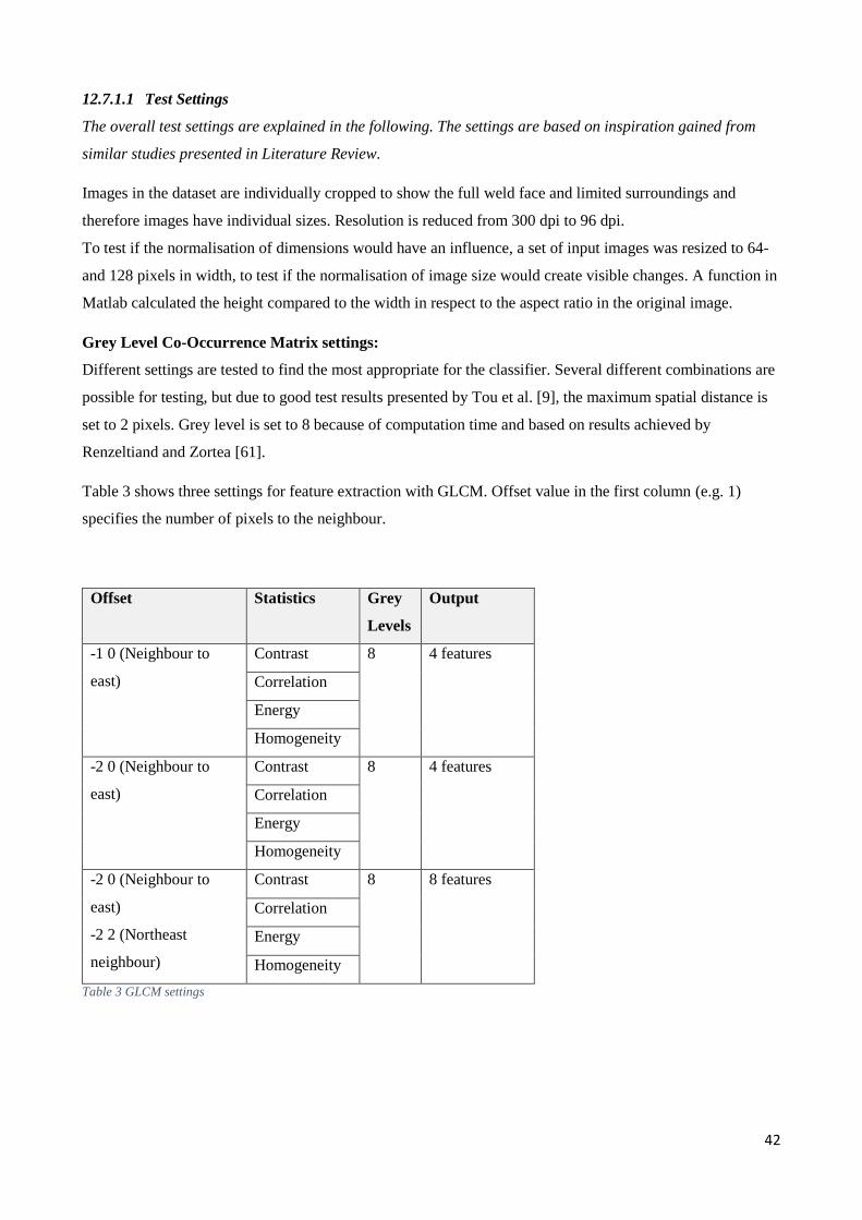
42
12.7.1.1 Test Settings
The overall test settings are explained in the following. The settings are based on inspiration gained from
similar studies presented in Literature Review.
Images in the dataset are individually cropped to show the full weld face and limited surroundings and
therefore images have individual sizes. Resolution is reduced from 300 dpi to 96 dpi.
To test if the normalisation of dimensions would have an influence, a set of input images was resized to 64-
and 128 pixels in width, to test if the normalisation of image size would create visible changes. A function in
Matlab calculated the height compared to the width in respect to the aspect ratio in the original image.
Grey Level Co-Occurrence Matrix settings:
Different settings are tested to find the most appropriate for the classifier. Several different combinations are
possible for testing, but due to good test results presented by Tou et al. [9], the maximum spatial distance is
set to 2 pixels. Grey level is set to 8 because of computation time and based on results achieved by
Renzeltiand and Zortea [61].
Table 3 shows three settings for feature extraction with GLCM. Offset value in the first column (e.g. 1)
specifies the number of pixels to the neighbour.
Offset Statistics Grey
Levels
Output
-1 0 (Neighbour to
east)
Contrast 8 4 features
Correlation
Energy
Homogeneity
-2 0 (Neighbour to
east)
Contrast 8 4 features
Correlation
Energy
Homogeneity
-2 0 (Neighbour to
east)
-2 2 (Northeast
neighbour)
Contrast 8 8 features
Correlation
Energy
Homogeneity
Table 3 GLCM settings
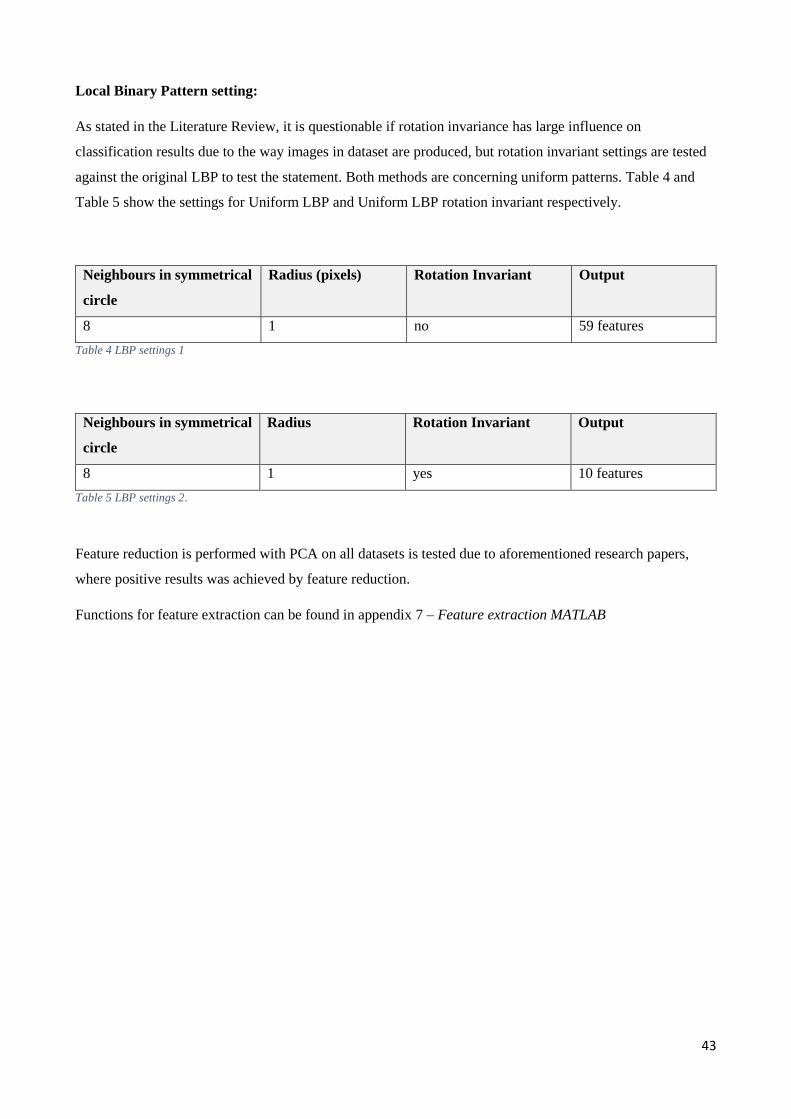
43
Local Binary Pattern setting:
As stated in the Literature Review, it is questionable if rotation invariance has large influence on
classification results due to the way images in dataset are produced, but rotation invariant settings are tested
against the original LBP to test the statement. Both methods are concerning uniform patterns. Table 4 and
Table 5 show the settings for Uniform LBP and Uniform LBP rotation invariant respectively.
Neighbours in symmetrical
circle
Radius (pixels) Rotation Invariant Output
8 1 no 59 features
Table 4 LBP settings 1
Neighbours in symmetrical
circle
Radius Rotation Invariant Output
8 1 yes 10 features
Table 5 LBP settings 2.
Feature reduction is performed with PCA on all datasets is tested due to aforementioned research papers,
where positive results was achieved by feature reduction.
Functions for feature extraction can be found in appendix 7 – Feature extraction MATLAB
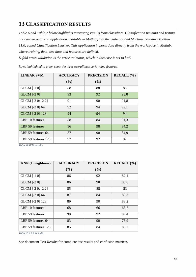
44
13 CLASSIFICATION RESULTS
Table 6 and Table 7 below highlights interesting results from classifiers. Classification training and testing
are carried out by an application available in Matlab from the Statistics and Machine Learning Toolbox
11.0, called Classification Learner. This application imports data directly from the workspace in Matlab,
where training data, test data and features are defined.
K-fold cross-validation is the error estimator, which in this case is set to k=5.
Rows highlighted in green show the three overall best performing features.
LINEAR SVM ACCURACY
(%)
PRECISION
(%)
RECALL (%)
GLCM [-1 0] 88 88 88
GLCM [-2 0] 93 92 93,8
GLCM [-2 0; -2 2] 91 90 91,8
GLCM [-2 0] 64 92 94 92,1
GLCM [-2 0] 128 94 94 94
LBP 10 features 88 84 91,3
LBP 59 features 96 98 94,2
LBP 59 features 64 87 90 84,9
LBP 59 features 128 92 92 92
Table 6 SVM results
KNN (1 neighbour) ACCURACY
(%)
PRECISION
(%)
RECALL (%)
GLCM [-1 0] 86 92 82,1
GLCM [-2 0] 86 90 83,6
GLCM [-2 0; -2 2] 85 88 83
GLCM [-2 0] 64 87 84 89,3
GLCM [-2 0] 128 89 90 88,2
LBP 10 features 68 66 68,7
LBP 59 features 90 92 88,4
LBP 59 features 64 83 90 78,9
LBP 59 features 128 85 84 85,7
Table 7 KNN results
See document Test Results for complete test results and confusion matrices.
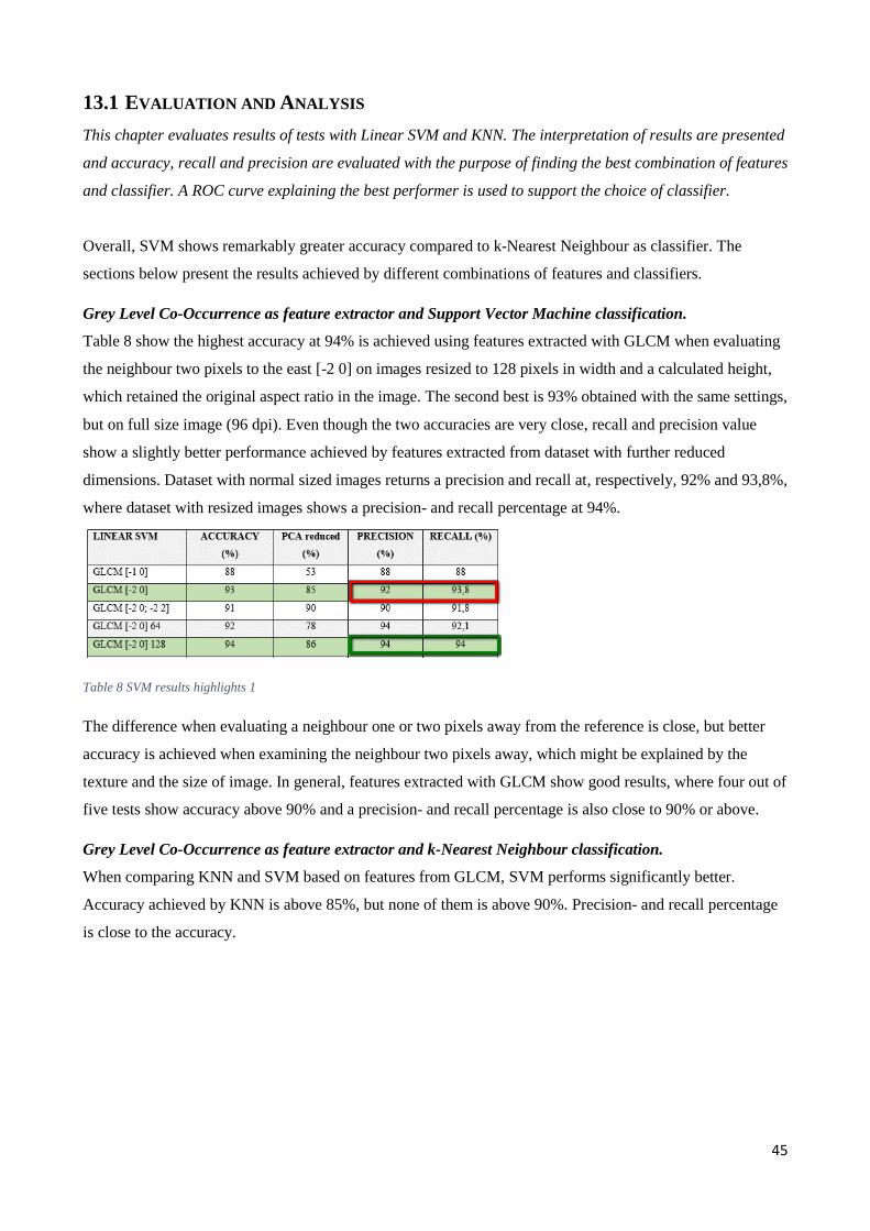
45
13.1 EVALUATION AND ANALYSIS
This chapter evaluates results of tests with Linear SVM and KNN. The interpretation of results are presented
and accuracy, recall and precision are evaluated with the purpose of finding the best combination of features
and classifier. A ROC curve explaining the best performer is used to support the choice of classifier.
Overall, SVM shows remarkably greater accuracy compared to k-Nearest Neighbour as classifier. The
sections below present the results achieved by different combinations of features and classifiers.
Grey Level Co-Occurrence as feature extractor and Support Vector Machine classification.
Table 8 show the highest accuracy at 94% is achieved using features extracted with GLCM when evaluating
the neighbour two pixels to the east [-2 0] on images resized to 128 pixels in width and a calculated height,
which retained the original aspect ratio in the image. The second best is 93% obtained with the same settings,
but on full size image (96 dpi). Even though the two accuracies are very close, recall and precision value
show a slightly better performance achieved by features extracted from dataset with further reduced
dimensions. Dataset with normal sized images returns a precision and recall at, respectively, 92% and 93,8%,
where dataset with resized images shows a precision- and recall percentage at 94%.
Table 8 SVM results highlights 1
The difference when evaluating a neighbour one or two pixels away from the reference is close, but better
accuracy is achieved when examining the neighbour two pixels away, which might be explained by the
texture and the size of image. In general, features extracted with GLCM show good results, where four out of
five tests show accuracy above 90% and a precision- and recall percentage is also close to 90% or above.
Grey Level Co-Occurrence as feature extractor and k-Nearest Neighbour classification.
When comparing KNN and SVM based on features from GLCM, SVM performs significantly better.
Accuracy achieved by KNN is above 85%, but none of them is above 90%. Precision- and recall percentage
is close to the accuracy.
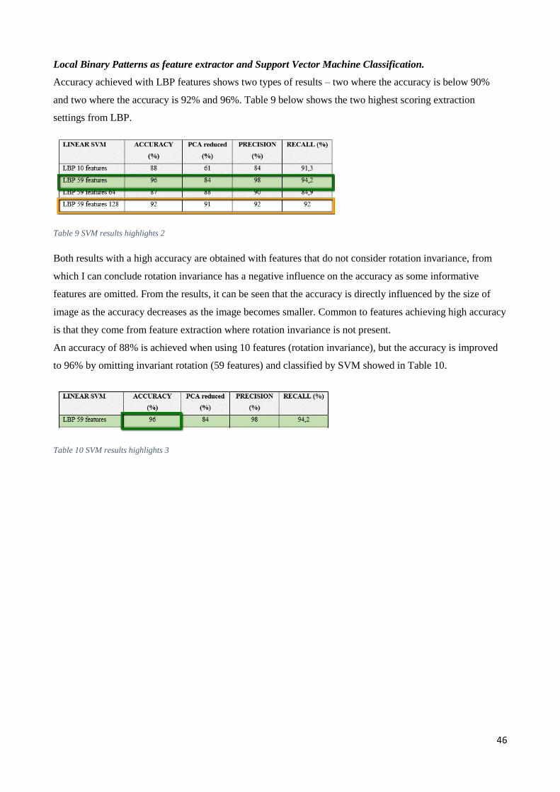
46
Local Binary Patterns as feature extractor and Support Vector Machine Classification.
Accuracy achieved with LBP features shows two types of results – two where the accuracy is below 90%
and two where the accuracy is 92% and 96%. Table 9 below shows the two highest scoring extraction
settings from LBP.
Table 9 SVM results highlights 2
Both results with a high accuracy are obtained with features that do not consider rotation invariance, from
which I can conclude rotation invariance has a negative influence on the accuracy as some informative
features are omitted. From the results, it can be seen that the accuracy is directly influenced by the size of
image as the accuracy decreases as the image becomes smaller. Common to features achieving high accuracy
is that they come from feature extraction where rotation invariance is not present.
An accuracy of 88% is achieved when using 10 features (rotation invariance), but the accuracy is improved
to 96% by omitting invariant rotation (59 features) and classified by SVM showed in Table 10.
Table 10 SVM results highlights 3
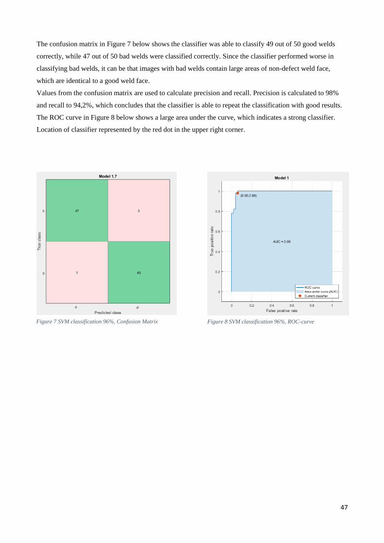
47
The confusion matrix in Figure 7 below shows the classifier was able to classify 49 out of 50 good welds
correctly, while 47 out of 50 bad welds were classified correctly. Since the classifier performed worse in
classifying bad welds, it can be that images with bad welds contain large areas of non-defect weld face,
which are identical to a good weld face.
Values from the confusion matrix are used to calculate precision and recall. Precision is calculated to 98%
and recall to 94,2%, which concludes that the classifier is able to repeat the classification with good results.
The ROC curve in Figure 8 below shows a large area under the curve, which indicates a strong classifier.
Location of classifier represented by the red dot in the upper right corner.
Figure 8 SVM classification 96%, ROC-curve Figure 7 SVM classification 96%, Confusion Matrix
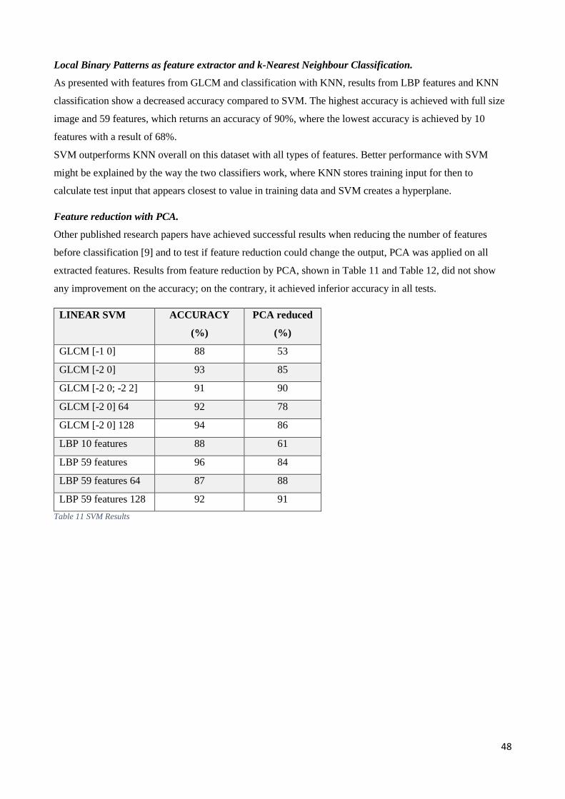
48
Local Binary Patterns as feature extractor and k-Nearest Neighbour Classification.
As presented with features from GLCM and classification with KNN, results from LBP features and KNN
classification show a decreased accuracy compared to SVM. The highest accuracy is achieved with full size
image and 59 features, which returns an accuracy of 90%, where the lowest accuracy is achieved by 10
features with a result of 68%.
SVM outperforms KNN overall on this dataset with all types of features. Better performance with SVM
might be explained by the way the two classifiers work, where KNN stores training input for then to
calculate test input that appears closest to value in training data and SVM creates a hyperplane.
Feature reduction with PCA.
Other published research papers have achieved successful results when reducing the number of features
before classification [9] and to test if feature reduction could change the output, PCA was applied on all
extracted features. Results from feature reduction by PCA, shown in Table 11 and Table 12, did not show
any improvement on the accuracy; on the contrary, it achieved inferior accuracy in all tests.
LINEAR SVM ACCURACY
(%)
PCA reduced
(%)
GLCM [-1 0] 88 53
GLCM [-2 0] 93 85
GLCM [-2 0; -2 2] 91 90
GLCM [-2 0] 64 92 78
GLCM [-2 0] 128 94 86
LBP 10 features 88 61
LBP 59 features 96 84
LBP 59 features 64 87 88
LBP 59 features 128 92 91
Table 11 SVM Results
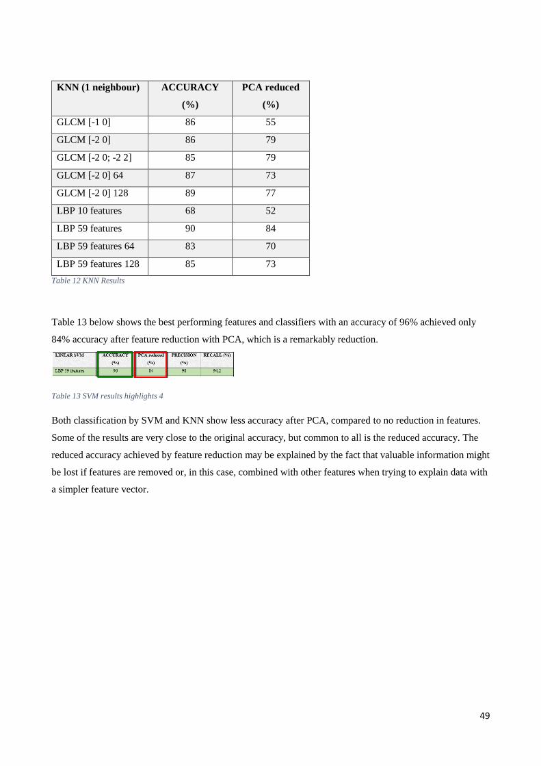
49
KNN (1 neighbour) ACCURACY
(%)
PCA reduced
(%)
GLCM [-1 0] 86 55
GLCM [-2 0] 86 79
GLCM [-2 0; -2 2] 85 79
GLCM [-2 0] 64 87 73
GLCM [-2 0] 128 89 77
LBP 10 features 68 52
LBP 59 features 90 84
LBP 59 features 64 83 70
LBP 59 features 128 85 73
Table 12 KNN Results
Table 13 below shows the best performing features and classifiers with an accuracy of 96% achieved only
84% accuracy after feature reduction with PCA, which is a remarkably reduction.
Table 13 SVM results highlights 4
Both classification by SVM and KNN show less accuracy after PCA, compared to no reduction in features.
Some of the results are very close to the original accuracy, but common to all is the reduced accuracy. The
reduced accuracy achieved by feature reduction may be explained by the fact that valuable information might
be lost if features are removed or, in this case, combined with other features when trying to explain data with
a simpler feature vector.
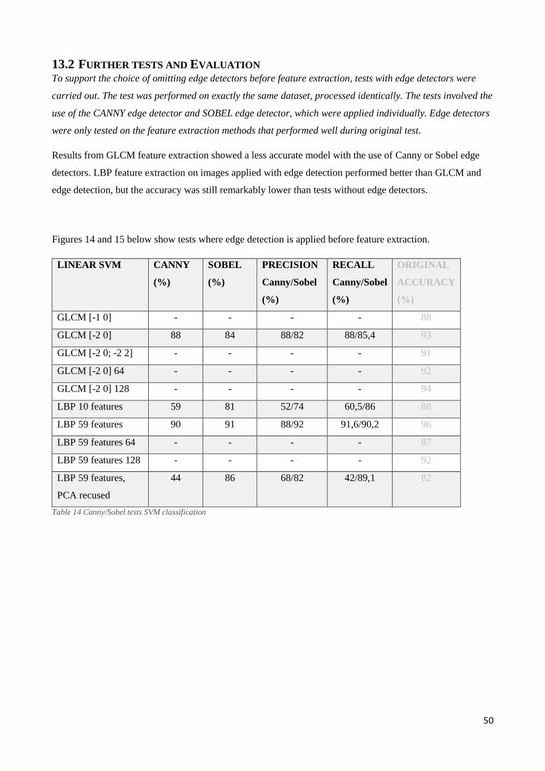
50
13.2 FURTHER TESTS AND EVALUATION To support the choice of omitting edge detectors before feature extraction, tests with edge detectors were
carried out. The test was performed on exactly the same dataset, processed identically. The tests involved the
use of the CANNY edge detector and SOBEL edge detector, which were applied individually. Edge detectors
were only tested on the feature extraction methods that performed well during original test.
Results from GLCM feature extraction showed a less accurate model with the use of Canny or Sobel edge
detectors. LBP feature extraction on images applied with edge detection performed better than GLCM and
edge detection, but the accuracy was still remarkably lower than tests without edge detectors.
Figures 14 and 15 below show tests where edge detection is applied before feature extraction.
LINEAR SVM CANNY
(%)
SOBEL
(%)
PRECISION
Canny/Sobel
(%)
RECALL
Canny/Sobel
(%)
ORIGINAL
ACCURACY
(%)
GLCM [-1 0] - - - - 88
GLCM [-2 0] 88 84 88/82 88/85,4 93
GLCM [-2 0; -2 2] - - - - 91
GLCM [-2 0] 64 - - - - 92
GLCM [-2 0] 128 - - - - 94
LBP 10 features 59 81 52/74 60,5/86 88
LBP 59 features 90 91 88/92 91,6/90,2 96
LBP 59 features 64 - - - - 87
LBP 59 features 128 - - - - 92
LBP 59 features,
PCA recused
44 86 68/82 42/89,1 82
Table 14 Canny/Sobel tests SVM classification
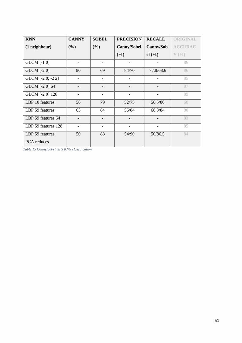
51
KNN
(1 neighbour)
CANNY
(%)
SOBEL
(%)
PRECISION
Canny/Sobel
(%)
RECALL
Canny/Sob
el (%)
ORIGINAL
ACCURAC
Y (%)
GLCM [-1 0] - - - - 86
GLCM [-2 0] 80 69 84/70 77,8/68,6 86
GLCM [-2 0; -2 2] - - - - 85
GLCM [-2 0] 64 - - - - 87
GLCM [-2 0] 128 - - - - 89
LBP 10 features 56 79 52/75 56,5/80 68
LBP 59 features 65 84 56/84 68,3/84 90
LBP 59 features 64 - - - - 83
LBP 59 features 128 - - - - 85
LBP 59 features,
PCA reduces
50 88 54/90 50/86,5 84
Table 15 Canny/Sobel tests KNN classification
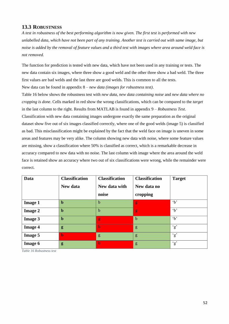
52
13.3 ROBUSTNESS A test in robustness of the best performing algorithm is now given. The first test is performed with new
unlabelled data, which have not been part of any training. Another test is carried out with same image, but
noise is added by the removal of feature values and a third test with images where area around weld face is
not removed.
The function for prediction is tested with new data, which have not been used in any training or tests. The
new data contain six images, where three show a good weld and the other three show a bad weld. The three
first values are bad welds and the last three are good welds. This is common to all the tests.
New data can be found in appendix 8 – new data (images for robustness test).
Table 16 below shows the robustness test with new data, new data containing noise and new data where no
cropping is done. Cells marked in red show the wrong classifications, which can be compared to the target
in the last column to the right. Results from MATLAB is found in appendix 9 – Robustness Test.
Classification with new data containing images undergone exactly the same preparation as the original
dataset show five out of six images classified correctly, where one of the good welds (image 5) is classified
as bad. This misclassification might be explained by the fact that the weld face on image is uneven in some
areas and features may be very alike. The column showing new data with noise, where some feature values
are missing, show a classification where 50% is classified as correct, which is a remarkable decrease in
accuracy compared to new data with no noise. The last column with image where the area around the weld
face is retained show an accuracy where two out of six classifications were wrong, while the remainder were
correct.
Data Classification
New data
Classification
New data with
noise
Classification
New data no
cropping
Target
Image 1 b b g ‘b’
Image 2 b b g ‘b’
Image 3 b g b ‘b’
Image 4 g b g ‘g’
Image 5 b g g ‘g’
Image 6 g b g ‘g’
Table 16 Robustness test

53
Robustness tests show a strong classifier on new unknown data, which have undergone the same treatment as
training data. A remarkably decreasing accuracy occurs when feature values are missing. A slightly better
accuracy is achieved when classifying new data, with images without a tight crop around the weld face. This
shows the function created by SVM is strong on new unknown data with same standard as the training data,
but with missing values a poor accuracy is obtained.

54
14 DISCUSSION
Between the two different types of classifiers used, SVM achieved the best results. The better accuracy
achieved by SVM might be explained by the categorisation of eager learners and lazy learners, where SVM
is an eager learner. The eager learner creates a model to explain test objects based on training data, while the
lazy learner stores the input from the training data, to then try to find a match between training and test data.
Several of the feature inputs have values close to each other due to the similarity in images, which might be
the answer to the lower accuracy with KNN classification.
To reduce the risk of overfitting, k-fold cross-validation is used. Cross-validation splits data into folds, so
some of the data is used for training and some is used for testing. The k value is individual for each type of
dataset, but cross-validation with five folds are used due to positive results in [58], [59] but other fold values
should be tested if further research is performed. Perhaps a number above five, but below ten would
contribute to better accuracy – although this is only an assumption.
The choice of SVM and KNN as classifiers was based on results from published papers within the area, but
also because they are two different types of classifiers. Further testing could be performed with another
classifier than KNN, since the classifier had the poorest performance. A robustness test with SVM showed a
strong classifier with new data, but data with missing values showed a poor accuracy of only 50%.
Decreasing accuracy with missing values during the robustness test might also explain the poor accuracy
when applying edge detection before feature extraction. When examining extracted features, several columns
show missing feature values and, related to the robustness test, the poor accuracy can be explained.
The level of the accuracy can always be discussed, and whether the accuracy scores highly enough. The level
of accuracy and the conclusion if it is high enough depends on the intended use, but also the expenses of
preparation. If expenses increase remarkably when trying to achieve 2% better accuracy it might be
discussed if the lower accuracy would be sufficient. Another aspect regarding the accuracy is intended use of
the welded object and the level of repair costs [1].
Images in the dataset were individually cropped to show weld face, but since images do not fulfil the same
standard regarding orientation, it was difficult to eliminate areas around the weld face. This issue might have
created unnecessary noise, which could have been avoided.
Due to the limited amount of time, samples in the dataset were created with defects simplified and more
distinguishable compared to real-life occurring faults. Defects are errors in gas supply, which means oxygen
is mixed in the weld pool with a porous weld face as a result. Oxygen mixed in the weld pool will show the
same output as the samples, but maybe less distinctively. This simplicity might have an influence on the
classification based on the features, but then again, the gas flaw only covers a small area on the weld face
and the rest of the image shows an approved weld face, which supports the simplified dataset.
It can be discussed if ROI would have contributed to a better performance and classification. For detection of
areas with poor weld in the image, ROI would definitely have been beneficial, but since the thesis concerns
55
classification, it was chosen not to be implemented. Images in dataset are cropped to show an absolute
minimum of the surroundings, which can, in some way, be presented as the ROI, because the full image is of
interest for the model.
It can always be contemplated if more tests are required to obtain a valid result, but due to the limited
working period, the test area had to be limited. Several different combinations of feature extraction methods
and classifiers can be combined in the search for an increase in percentage accuracy. Within the tested
methods, several different settings can be applied, which opens up the area even more. Test settings were
chosen based on successful test results in published papers, which was used as validation of settings applied.
If further testing is performed, other test settings should be evaluated in order to find the most suitable, even
though an accuracy of 96% was achieved.
Images in the dataset were of a difference size and normalisation of dimensions were evaluated. The length
of the weld samples was approximately ten centimetres and the defects are situated randomly within this
length, and a normalisation of the length would, in some cases, result in cropping in the defected area and
therefore normalisation of the width only was performed. If new dataset is created a better standardization of
samples should be applied.
Offset value used for both GLCM and LBP is based on test results presented in published papers (presented
in the Literature Review) and best accuracy was achieved by LBP evaluating the first neighbour, while
GLCM achieves better results when looking at the second neighbour. It was not tested if LBP feature
extraction would perform better if evaluating second or third neighbour, but this should be performed if
tested further.
Robustness is a way of testing how the classifier handles, for example, noisy data, and how it affects the
result. Since images in dataset do not follow an identical standard, i.e. they have individual dimensions, it
can be discussed if this can tell something about the robustness, but best accuracy in this case is achieved
with downscaled images (tight crop around weld face). During the robustness test, new data that were not
used during any training were tested in the classifier, where the results showed a strong classifier on new
unknown data, but a decreasing accuracy when feature values were missing, which explains the importance
of all features extracted. This might also explain the lower accuracy when applying feature reduction before
classification.
Since images in the dataset aim to follow the same standards, such as the orientation of weld face, it is
discussed if rotation invariance during LBP features extraction is necessary. Good results were obtained
when extracting features with rotation invariant LBP on Brodatz’s dataset, where some images in dataset
were tilted [9]. Since some of the images in the dataset tend to tilt, it would have seemed obvious that good
results should be present with rotation invariance, but results show the opposite. Perhaps this is because all
images show the same type of structure, while Brodatz’s contain several different surface textures.
Many different validation methods are available and the use of cross-validation, with 5-fold validation, is
based on experience from other research papers, but due to a relatively small dataset (50 good and 50 bad)
56
leave one out validation might also have contributed to high accuracy. This is not tested since high accuracy
was achieved with 5-fold validation, but should be tested in further work.
When evaluating results from datasets with full-size images and datasets where normalisation of width was
performed, the performance was very close and normalisation of dimensions can be discussed. This should
only be concerned when dealing with images with little variance in dimensions and where ROI is
approximately the same size.
As mentioned, tests with Canny and Sobel edge detectors showed poor classification results, but another
option to implement the use of edge detection could be a transition of grey scale images and images showing
only weld edges. This combination might create strong features because it combines information from the
surface, but also from the highlighted edges of the weld. An unbroken line of white pixels represents the
edge, but if a grouping of white pixels occurs between edge lines, it may explain a defect on the surface.
Another way to use edge detectors could be to count white pixels in the image.
There are many different approaches to this subject and the type of classification, which means there are also
many methods that can be used. Feature extraction methods and classifiers were chosen based on results in
evaluated research papers and it is conjecture whether another method might have achieved better results.
The model presented acts only as the prototype to test if this type of feature extraction can create valuable
information about the weld face. The idea behind it was that something similar could be installed as a
permanent setup on a linear welding rack, where images are obtained automatically. Combining image
processing and evaluation is performed and if a defect occurs, the image is saved and sent to manual
evaluation where decision regarding next step is taken.

57
15 CONCLUSION
As stated in Problem Statement this thesis attempts to find a model to classify simple surface defects in MIG
welds. This is pursued in order to reduce the use of skilled labour as part of the general visual inspection.
The two promising features extraction methods are tested and evaluated based on the accuracy achieved by
two classification methods.
A method for visual inspection of MIG weld with gas flaws is presented based on feature extraction and
classification algorithms. Feature extraction methods (Grey Level Co-Occurrence & Local Binary Patterns)
are evaluated based their ability to describe surface textures, which are used for classification purposes. Two
classification methods (Support Vector Machine & k-Nearest Neighbour) are compared to find the best
suitable classifier for the data.
Best classification results are obtained with a SVM, full-size images (96 dpi) and features extracted by
uniform LBP. Images are only cropped to show weld face and dimensions are individual for every image.
Tests with normalised images, feature reduction and edge detection methods are performed, but the best
results were found with images downscaled from 300 dpi to 96 dpi.
The highest accuracy of 96% is achieved with a combination of LBP features and SVM classification.
This work presents a prototype, which only concerns features extraction methods and classifiers, which
means a fully automated model is not presented.
16 FURTHER WORK
This chapter presents ideas and thoughts behind further work within the area.
The next stage of this work should be to extend it to look at several types of flaws and defects. Detection and
evaluation of, for instance, undercuts, weld roots or alignment could be areas for further investigation. It is
believed that the created dataset is useful for this type of work as the welds show other minor flaws.
A test environment where a linear guided welding is performed and with a permanent camera setup could be
part of next step in the search for a fully automated detection model.
The idea of examining weld surfaces based on texture features creates a foundation for further research
regarding colour shadings and tempering around weld face. Could similar methods be used in colour
detection as an aid in the selection of tempering treatment?
58
17 BIBLIOGRAPHY
[1] G. Wang and T. W. Liao, “Automatic identification of different types of welding defects in,” NDT&E
International, p. 9, 2002.
[2] DanRobotics, “DanRobotics Welding robots,” 9 January 2016. [Online]. Available:
http://danrobotics.dk/svejserobotter/.
[3] G. E. Cook, R. J. Barnett, K. Andersen, J. F. Springfield and A. M. Strauss, “Automated Visual
Inspection and Interpretation,” Vanderbilt University, School of Engineering, Nashville, 1995.
[4] S. W. Lawson and G. A. Parker, “Automatic detection of defects in industrial ultrasound images using
a neural network,” Surrey, 1996.
[5] I. -. I. O. f. Standardization, “Non-destructive testing of welds - Radiographic testing of fusionwelded,”
ISO - International Organization for Standardization, Geneva, 2003.
[6] I. -. I. O. f. Standardization, “Non-destructive testing of welds - Ultrasonic Testing of Welded Joints,”
ISO - International Organization for Standardization, Geneva, 2005.
[7] O. Haffner and Š. Kozák, “PROPOSAL OF WELD DIAGNOSTIC AND EVALUATION METHOD,”
Bratislava, Slovak Republic, 2015.
[8] Weldingtypes, “Welding Types,” 2017. [Online]. Available: http://www.weldingtypes.net/. [Accessed
26 January 2017].
[9] J. Y. Tou, Y. H. Tay and P. Y. Lau, “Gabor filters and grey-level co-occurrence matrices in texture
classification.,” MMU International Symposium on Information and Communications Technologies,
pp. 197-202, November 2007.
[10] J. Hassan, A. M. Awan and A. Jalil, “Welding Defect Detection and Classification Using Geometric
Features,” Islamabad, 2012.
[11] Y. Xu, H. Yu, J. Zhong, T. Lin and S. Chen, “Real-time seam tracking control technology during
welding robot GTAW process,” Journal of Materials Processing Technology, vol. 212, no. 8, p. 8,
2012.
[12] D. Mery and M. A. Berti, “Automatic detection of welding defects,” International Symposium on
Computed Tomography and Image Processing for Industrial Radiology, vol. 45, no. 10, p. 9, 2003.
[13] B. Pathak and D. Barooah, “Tecture Analysis Based on the Grey Level Co occurence Matrix
considering possible orientations,” International Journal of Advanced Research in Electrical,
Electronics and Instrumentation Engineering, vol. 2, no. 9, p. 7, 2013.
[14] M. M. Hittawe, S. M. Muddamsetty, D. Sidibé and F. M´eriaudeau, “Multiple feature extraction for
timber defects detection and classification using SVM,” Le Creusot, France, 2015.
[15] C. D and C. B., “Semi-structured Interviews,” Qualitative Research Guidelines Project.", p. 2, 2008.
59
[16] J. Kumar, R. Anand and S. Srivastava, “Multi Class Welding Flaws Classification using Texture
Feature for Radiographic Images,” India, 2014.
[17] R. M. Haralick, K. Shanmugam and I. Dinstein, “Textural Features for Image Classification,” IEEE
TRANSACTIONS ON SYSTEMS, MAN, AND CYBERNETICS,, vol. 3, no. 6, p. 12, 1973.
[18] P. Mohanaiah, P. Sathyanarayana and L. GuruKumar, “Image Texture Feature Extraction Using
GLCM Approach,” International Journal of Scientific and Reseach Publication, vol. 3, no. 5, p. 5,
2013.
[19] R. R. d. Silva, L. P. Calôba, M. H. Siqueira and J. M. Rebello, “Pattern recognition of weld defects
detected by radiographic test,” NDT&E International, vol. 37, p. 9, 2004.
[20] T. Ojala, M. Pietikäinen and D. Harwood, “A Comparative Study of Texture Measures with
Classification based on Feature Distributions,” Pattern Recoonition,, vol. 29, no. 1, p. 8, 1996.
[21] V.-L. Nguyen, N.-S. Vu and P.-H. Gosselin, “A Scattering Transform combination with Local Binary
Pattern for Texture Classification,” Cergy, France, 2016.
[22] Z. Guo, L. Zhang and D. Zhang, “A Completed Modeling of Local Binary Pattern Operator for Texture
Classification,” IEEE Transactions on Image Processing, vol. 19, no. 6, p. 6, 2010.
[23] T. Ojala, M. Pietikäinen, IEEE and T. Maäenpää, “Multiresolution Grey-Scale and Rotation Invariant
Texture Classifcation with Local Binary Patterns,” IEEE TRANSACTIONS ON PATTERN ANALYSIS
AND MACHINE INTELLIGENCE, vol. 24, no. 7, p. 17, 2002.
[24] B. Gudla, S. R. Chalamala and S. K. Jami, “Local Binary Patterns For Gender Classification,” 2015.
[25] C. Cortes and V. Vapnik, “Support Vector Networks,” in Machine Learning, L. Saitta, Ed., Boston,
Kluwer Academic Publishers, 1995, p. 20.
[26] H. Meng, H. Xu and Q. Tan, “Fault Diagnosis Based on Dynamic SVM,” Nanjing, China, 2016.
[27] T. Murosaki, KuniyasuYoshida and HirokiNaganuma, “Visual Inspection with SVM,” Tokyo, 2008.
[28] M. Ahmed, A. Shaukat and M. U. Akram, “Comparative Analysis of Texture Descriptors for
Classification,” Islamabad, Pakistan, 2016.
[29] D. M. Ideler, “Comparison of Artificial Neural Network and k-Nearest Neighbour for Classification,”
Brock, Cananda.
[30] J. N. Pires, A. Loureiro, T. Godinho, P. Ferreira, B. Fernando and J. Morgado, “Welding Robots,”
IEEE Robotics & Automation Magazine, p. 11, June 2003.
[31] L. Denver, “Types of welding procedures,” 2017. [Online]. Available:
http://www.lincolntech.edu/news/skilled-trades/welding-technology/types-of-welding-procedures.
[Accessed 26 January 2017].
[32] EWP, “Welding Joints - Butt welded & Fillet welded Joints,” 2017. [Online]. Available:
http://www.wermac.org/others/welding_basic-welding-joints_butt-weld_fillet-weld.html. [Accessed 27
January 2017].
60
[33] A. B.G., “THE 5 TYPES OF BASIC WELDING JOINTS,” 2014. [Online]. Available:
http://www.ateliersbg.com/news/the-5-types-of-basic-welding-joints.aspx. [Accessed 27 January
2017].
[34] K. G. Bøving, NDE Handbook: Non-Destructive Examination Methods for Condition Monitoring,
Revised ed., Elsevier, 2014.
[35] I. -. I. O. f. Standardization, “Non-destructive testing of welds - Visual Testing of fusion-welded
joints,” ISO - International Organization for Standardization, Geneva, 2003.
[36] I. O. o. Standardization, Welding — Fusion-welded joints in steel,, Geneva: ISO, 2014.
[37] I. O. o. Standardization, “Defects accoring ISO 6520,” Standardization, International Organisation of,
Geneva, 2010.
[38] I. -. I. O. f. Standardization, “Non-destructive testing of welds - Ultrasonic testing - Use of time-of-
flight diffraction technique (TOFD),” ISO - International Organization for Standardization, Geneva,
2011.
[39] L. A. Chan and S. Z. Der, “Neural-Based Target Detectors for,” in Image Recognition and
Classification Algorithms, Systems, and Applications, B. Javidi, Ed., New York, Marcel Dekker Inc.,
2002, pp. 1-36.
[40] Z. Othman, H. Haron and M. R. A. Kadir, “Comparison of Canny and Sobel Edge Detection in MRI
Images,” in IEEE, Kuala Lumpur, 2008.
[41] D. A. Clausi, “An analysis of co-occurrence texture statistics as a function of grey level quantization,”
Can. J. Remote Sensing,, vol. 28, no. 1, p. 17, 2002.
[42] B. S. V, A. Unnikrishnan and K. Balakrishnan, “GREY LEVEL CO-OCCURRENCE MATRICES:
GENERALISATION AND SOME NEW FEATURES,” International Journal of Computer Science,
Engineering and Information Technology (IJCSEIT), vol. 2, no. 2, p. 7, 2012.
[43] M. Yang, K. Kpalma and J. Ronsin., “A Survey of Shape Feature Extraction Techniques,” Peng-Yeng
Yin. Pattern Recognition, IN-TECH, p. 47, 2008.
[44] R. Jobanputra and D. A. Clausi, “Preserving boundaries for image texture segmentation using grey
level co-occurring probalities,” The journal of pattern recognisition society, vol. 39, no. 2, p. 12, 2005.
[45] I. MathWorks, “Texture Analysis Using the Gray-Level Co-Occurrence Matrix (GLCM),” 2017.
[Online]. Available: https://se.mathworks.com/help/images/gray-level-co-occurrence-matrix-
glcm.html. [Accessed 20 February 2017].
[46] B.-h. Wang, H.-j. Wang and H.-n. Qi, “Wood Recognition Based on Grey-Level Co-Occurrence
Matrix,” Taiyuan, 2010.
[47] I. Mathworks, “graycoprops,” 2016. [Online]. Available:
https://se.mathworks.com/help/images/ref/graycoprops.html. [Accessed 4 April 2017].
[48] I. Mathworks, “Local Feature Detection and Extraction,” 2016. [Online]. Available:
https://se.mathworks.com/help/vision/ug/local-feature-detection-and-extraction.html. [Accessed 4
April 2017].
61
[49] M. Pietikäinen, G. Zhao, A. Hadid and T. Ahonen, “Mappings of the LBP Labels: Uniform Patterns,”
in Computer Vision Using Local Binary Patterns, New York, Springer London Dordrecht Heidelberg,
2011, p. 213.
[50] I. Guyon and A. Elisseeff, “An Introduction to Variable and Feature Selection,” p. 26, 2003.
[51] Mathworks, “Principal Component Analysis,” Mathworks, 2016. [Online]. Available:
https://se.mathworks.com/help/stats/principal-component-analysis-pca.html. [Accessed 24 April 2017].
[52] M. I. Jordan and T. M. Mitchell, “Machine learning: Trends, perspectives, and prospects,” Science ,
vol. 349, pp. 255-260, 2015.
[53] I. H. Witten, E. Frank and M. A. Hall, Data Mining, Practical Machine Learning Tools and
Techniques, Third ed., Burlington: Elsevier Inc., 2011.
[54] J. Han, M. Kamber and J. Pei, Data Mining, Concepts and Techniques, Third ed., Waltham: Morgan
Kaufmann, 2012.
[55] A. A. Moghaddam, “Image Processing Techniques for Classification of Linear Welding Defects,” in
IEEE , Tehran, Iran, 2015.
[56] N. Gerard, “Data Mining - Support Vector Machines (SVM) algorithm,” Boostrap, 21 March 2017.
[Online]. Available:
https://gerardnico.com/wiki/data_mining/support_vector_machine#support_vectors. [Accessed 11 May
2017].
[57] XindongWu, V. Kumar, J. R. Quinlan, J. Ghosh, Q. Yang, H. Motoda, G. J. McLachlan, A. Ng, B. Liu,
P. S. Yu, Z.-H. Zhou, M. Steinbach, D. J. Hand and D. Steinberg, “Top 10 algorithms in data mining,”
in IEEE, 2007.
[58] N. Gerard, “Machine Learning - Rote Classifier,” Boostrap, 21 March 2017. [Online]. Available:
https://gerardnico.com/wiki/data_mining/rote. [Accessed 11 May 2017].
[59] S. Arlot and A. Celisse, “A survey of cross-validation procedures for model selection,” Statistics
Surveys, vol. 4, p. 39, 2010.
[60] R. Kohavi, “A Study of Cross-Validation and Bootstrap for Accuracy Estimation and Model
Selection,” in International Joint Conference on Artificial intelligence , Quebec, 1995.
[61] J. Davis and M. Goadrich, “The Relationship Between Precision-Recall and ROC Curves,” in
Proceedings of the 23rd international conference on Machine learning, Pittsburg, 2006.
[62] F. Renzettiand and L. Zortea, “Use of a gray level co-occurrence matrix to characterize duplex
stainless steel phases microstructure,” Frattura ed Integrita Strutturale, vol. 16, p. 43, 2011.
[63] G. Wang and T. W. Liao, “Automatic identification of different types of welding defects in,” NDT&E
International, no. 35, p. 10, 2002.
[64] M. M. Silva, F. C. Cruz, P. C. M. A. Farias, E. F. S. Filho, M. C. S. Albuquerque, I. C. d. Silva and C.
T. T. Farias, “Neural decision support system for ultrasound nondestructive evaluation embedded in a
DSP,” 2015.

62
[65] G. Zhang, Z. M. Ma, Q. Tong, Y. He and T. Zhao, “Shape Feature Extraction Using Fourier
Descriptors with Brightness in,” 2008.
[66] D. Mery and M. A. Berti, “Automatic detection of welding defects,” Berlin, 2003.
[67] M. Rouse, “Definition machine learning,” February 2016. [Online]. Available:
http://whatis.techtarget.com/definition/machine-learning. [Accessed 5 11 2016].
[68] R. Jobanputra and D. A. Clausi, “Preserving boundaries for image texture segmentation using grey
level co-occurring probalities,” Pattern Recognition, The Journal of Pattern Recognition Society, vol.
39, p. 11, 2006.
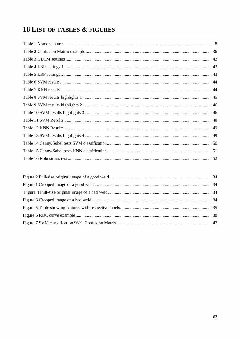
63
18 LIST OF TABLES & FIGURES
Table 1 Nomenclature ....................................................................................................................................... 8
Table 2 Confusion Matrix example ................................................................................................................. 36
Table 3 GLCM settings ................................................................................................................................... 42
Table 4 LBP settings 1 .................................................................................................................................... 43
Table 5 LBP settings 2. ................................................................................................................................... 43
Table 6 SVM results ........................................................................................................................................ 44
Table 7 KNN results ........................................................................................................................................ 44
Table 8 SVM results highlights 1 .................................................................................................................... 45
Table 9 SVM results highlights 2 .................................................................................................................... 46
Table 10 SVM results highlights 3 .................................................................................................................. 46
Table 11 SVM Results ..................................................................................................................................... 48
Table 12 KNN Results ..................................................................................................................................... 49
Table 13 SVM results highlights 4 .................................................................................................................. 49
Table 14 Canny/Sobel tests SVM classification .............................................................................................. 50
Table 15 Canny/Sobel tests KNN classification .............................................................................................. 51
Table 16 Robustness test ................................................................................................................................. 52
Figure 2 Full-size original image of a good weld ............................................................................................ 34
Figure 1 Cropped image of a good weld ......................................................................................................... 34
Figure 4 Full-size original image of a bad weld ............................................................................................. 34
Figure 3 Cropped image of a bad weld ............................................................................................................ 34
Figure 5 Table showing features with respective labels. ................................................................................. 35
Figure 6 ROC curve example .......................................................................................................................... 38
Figure 7 SVM classification 96%, Confusion Matrix ..................................................................................... 47


![Visual Weld Inspection Guidelines Attachment A - …2].pdf · Visual Weld Inspection Guidelines Attachment A ... approved weld inspector shall document weld inspection results using](https://img.pdfslide.net/doc/110x75/5a78aa797f8b9a21538b97b6/visual-weld-inspection-guidelines-attachment-a-2pdfvisual-weld-inspection.jpg)