WELDING PROCESS OPTIMIZATION WITH ARTIFICIAL NEURAL ... · PDF fileWELDING PROCESS OPTIMIZATION WITH ARTIFICIAL NEURAL NETWORK ... paper presents a new modeling approach on prediction

WELDING PROCESS OPTIMIZATION WITH

ARTIFICIAL NEURAL NETWORK

APPLICATIONS

Adnan Aktepe∗, Suleyman Ersoz∗, Murat Luy†

Abstract: Correct detection of input and output parameters of a welding pro-cess is significant for successful development of an automated welding operation.In welding process literature, we observe that output parameters are predictedaccording to given input parameters. As a new approach to previous efforts, thispaper presents a new modeling approach on prediction and classification of weldingparameters. 3 different models are developed on a critical welding process basedon Artificial Neural Networks (ANNs) which are (i) Output parameter prediction,(ii) Input parameter prediction (reverse application of output prediction model)and (iii) Classification of products. In this study, firstly we use Pareto Analysisfor determining uncontrollable input parameters of the welding process based onexpert views. With the help of these analysis, 9 uncontrollable parameters aredetermined among 22 potential parameters. Then, the welding process of ammu-nition is modeled as a multi-input multi-output process with 9 input and 3 outputparameters. 1st model predicts the values of output parameters according to giveninput values. 2nd model predicts the values of correct input parameter combina-tion for a defect-free weld operation and 3rd model is used to classify the productswhether defected or defect-free. 3rd model is also used for validation of resultsobtained by 1st and 2nd models. A high level of performance is attained by all themethods tested in this study. In addition, the product is a strategic ammunition inthe armed forces inventory which is manufactured in a limited number of countriesin the world. Before application of this study, the welding process of the productcould not be carried out in a systematic way. The process was conducted by trial-and-error approach by changing input parameter values at each operation. Thiscaused a lot of costs. With the help of this study, best parameter combination isfound, tested, validated with ANNs and operation costs are minimized by 30%.

Key words: Artificial neural networks, welding process control, weld operation

Received: March 8, 2013 DOI: 10.14311/NNW.2014.24.037Revised and accepted: December 17, 2014

∗Adnan Aktepe – Corresponding Author, Suleyman Ersoz, Kirikkale University, Faculty ofEngineering, Department of Industrial Engineering, Yahsihan, Kirikkale, Turkey, Tel.: +90 318357 42 42–1047, Fax: +90 318 357 24 59, E-mail: [email protected], [email protected]

†Murat Luy, Kirikkale University, Faculty of Engineering, Department of Electric/ElectronicEngineering, Yahsihan, Kirikkale, Turkey, E-mail: [email protected]

c⃝CTU FTS 2014 655

Neural Network World 6/14, 655-670

1. Introduction

Control of the input and output parameters are important problems for weldingprocesses. This is a multi-input multi-output process. In order to control theprocess, the interaction among input and output parameters must be predicted.The problems for which a linear model cannot be built are examples of those kindsof problems. In addition, the mass number of parameters in the model increasesthe run time of the algorithms so that AI techniques are used for practical solution.

In the literature, statistical and numerical techniques are used for optimiza-tion of welding processes [2]. In their study, factorial design, linear regression,response surface methodology, Taguchi experimental design, Artificial Neural Net-work (ANN) and hybrid techniques are used for handling the welding process con-trol problem. For example, expert systems are used for classification of weldingdefect types [7]. In another study, a comparison is conducted among results ofGenetic Algorithms (GA), Simulated Annealing (SA) and ANN for stainless steelwelding process [17]. In their studies, the effect of input parameters such as heatingtime, heating pressure, upset pressure and upset time on output variables such astensile strength and metal loss are discussed.

ANN models provide effective solution approach to problems faced in materialscience. ANN models have a wide application area on casting, welding, analysisof interaction among input and output parameters and analysis of quality controlspecifications. ANN models on welding process control are summarized in theTab. I below.

In the literature it is observed that welding process control problem is mostlysolved for one aspect: Output parameter prediction. However in our study we ad-dress the problem with 3 different approaches: Output parameter prediction, inputparameter prediction and classification. We develop 3 different ANN applicationsfor welding process control of the product. 1st model is used for prediction of out-put parameters according to given input parameter values. Here the objective is tofind the value of output parameters before production and determine whether theproduct will is defected or not. 2nd model is used for input parameter prediction(reverse of Model 1). This model helped us to find the best input parameter com-bination for producing a non-defective product. Finally 3rd model is developed forclassification of products as defective or non-defective according to input parametervalues.

The models are applied on 155 mm artillery ammunition, which is producedin Mechanical and Chemical Industry Corporation (MKEK) Ammunition Factory,located in Turkey. In the welding process there were critical problems (which aredetailed in the next section) and 30% of the products were defective. With ourstudy now this ratio is decreased to 1–2% with great success and minimum errorrates. The paper is organized as follows: In the next section we give informationabout the welding process control problem. In the 3rd section solution approach isgiven with reduced number of uncontrollable input parameters. In the 4th sectionwe discuss ANN applications and in the last section we finalize the paper withconcluding remarks.

656

Aktepe A., Ersoz S., Luy M.: Welding process optimization . . .

Authors Year Scope of the study

Type of StudyOutput Input

parameter parameter Classificationprediction prediction

[19] 1997 Welding process model-ing and optimization

+

[5] 2004 Optimization of control-ling robotic arc welding

+

[8] 2005 Laser welding defect di-agnosis

+

[13] 2007 A novel system which al-lows arc-welding defectdetection and classifica-tion

+ +

[10] 2007 Defect detection in spotwelding

+

[1] 2007 A novel technique basedon ANN for prediction ofgas metal arc welding pa-rameters

+

[15] 2008 A multilayer neuralnetwork model to pre-dict the ultimate tensilestress (UTS) of weldedplates

+

[20] 2009 Prediction of mechanicalproperties of Cu-Sn-Pb-Zn-Ni alloys

+

[11] 2010 Prediction of stainlesssteel spot welding pa-rameters

+

Tab. I Summary of literature on ann models developed for solving welding problems.

2. Welding Problem

In the welding process a rotating band is welded to the body of ammunition. Afterwelding channel is created on the body in a Computer Numerically Controlled(CNC) station, it is transferred to the welding machine. After preheating operation,the body is transferred to the welding workbench. In this station, firstly the bodyis tied between stitch and panel. Then rotating manually, the welding channelis rubbed down, cleaned by an alcohol-soaked cloth and the body gets ready forwelding operation. Meanwhile copper and brass wires are prepared. The weldingmachine gets these wires and welding operation is realized with these metals. Aftercleaning process on the body, the torch distances for copper and brass wires, waterdischarge, gaseous fill rate, copper and brass wires’ speed, torch-nozzle distance arecontrolled and values are entered to the control panel manually. Finally weldingoperation starts. Welding operation carried out in the welding workbench is a

657


gas metal arc welding. The operation is carried out creating arc between Argongas and metal wires. This type of welding is also called Metal Inert Gas (MIG)welding. When the welding operation is started, firstly an arc is formed at thetorch where copper metal wire meets. And after 3-4 oscillations, as a second torchwith brass metal wire, an alloy is created in weld zone. When the torches make120-140 oscillations where copper and brass metal wires meet, weld zone is filledand the operation ends automatically. After welding operation the ammunitionbody is picked up from welding workbench and weld zone is grinded at beginning,middle and end parts. A chemical analysis is applied to these three zones. Inquality control operation, the zinc (ZnR), iron (FeR) and copper ratio (CuR) ofweld is measured. According to quality control specifications, metal ratios in theweld must be between lower and upper limits. For a defect-free weld ZnR must bebetween 8–12%, FeR must be between 0.5–4% and CuR must be between 84–91.5%.

The rotating band is the part that enables the ammunition to rotate in thebarrel and it affects the velocity and quality of the ammunition. After weldingtreatment, the metal proportions (ZnR, FeR, CuR) in the weld region must be atthe required level. For a defective product, for example if the iron ratio is lower,the rotating band may detach in the barrel. If the ratio is higher, the barrel maybe ruined.

In the current situation, the loss rates in the production are high for 155 mmartillery ammunition. There are problems about production of the product thathas been produced since January 1st 2009. The main problem is: The interactionamong input and output parameters of welding process cannot be predicted andtherefore optimum parameter configuration cannot be found.

The product is highly demanded due to its strategic importance and becauseof the problems in welding process, more than 50% of the annual demand cannotbe matched. In addition, because 30% of the products are defective, the reproduc-tion and salvage costs are incurred. The product cannot be used when it doesn’tsatisfy the quality requirements and only 18% of the defective products can beretrieved. The retrieval costs are incurred because of retrieval processes. After re-trieval processes, if ZnR, FeR and CuR are not in the specified level, the productsare scrapped and the retrieval process cannot be applied to these products for thesecond time. The scrap rate after retrieval process is 2%. In other words, for 18%of the products retrieval costs are incurred, for 10% of the products scrap costs areincurred and for 2% of the products both retrieval and scrap costs are incurred.

3. Parameter Analysis

For solving the welding problems discussed in the previous section, firstly the inputparameters are analyzed with experts (a group of 10 people consisting mechanical,industrial and chemical engineers-with managers of the factory). The input analysisprocess is carried out with Pareto Analysis. Pareto Analysis is a simple quality tool.It is a graphical method of comparing and sorting a set of measures. Pareto Analysisuses the ‘80/20 Rule’ to select the ‘vital few’ items for further action [14]. Benefitingfrom this property of Pareto Analysis we detected the controllable (unimportant)and uncontrollable (important) parameters of the model (Pareto Analysis resultsare shown on Fig. 1. The x-axis shows the number of input variables given in

658


Tab. II). In Tab. II, the list of 22 input parameters, output parameters and thereduced list of parameters found with Pareto Analysis are displayed (Uncontrollableinputs are in grey).

Fig. 1 Results of Pareto analysis.

The input parameters are evaluated by expert team with an evaluation form.Each expert gave scores for each parameter between 1 to 10 according to character-istic of the input. If the input is controllable the importance scores were low, if theinput is uncontrollable the scores were high. This evaluation is carried out to findthe uncontrollable parameters because there is no need of modeling for manuallycontrollable parameters.

After determining 9 uncontrollable input parameters and previously known out-put parameters, 3 different ANN models are developed. Fig. 2 summarizes thesolution approach developed in this study.

4. Neural Network Models Developed for WeldingProcess Control

In this study, 3 different models have been developed for welding process controlproblem defined in Section 2. For solving addressed problems, BackpropagationNeural Networks (BPNN) are used in the study. Model 1 is used for output pa-rameter prediction, Model 2 is used to predict input parameter values given the

659


INPUT PARAMETERS

No Input Name Input Unit Uncontrollable

V.1 Chemical analysis of copper wire-I CCW1 %

V.2 Chemical analysis of copper wire-II CCW2 %

V.3 Chemical analysis of copper wire-III CCW3 %

V.4 Zinc ratios of brass wire ZBW %

V.5 Copper ratio of brass wire CBW %

V.6 Brass wire drawing speed BDS m/min +

V.7 Copper wire drawing speed CDS m/min +

V.8 Brass torch rate BTR mm

V.9 Copper torch rate CTR mm +

V.10 Brass torch angle BTA angle

V.11 Copper torch angle CTA angle +

V.12 Furnace temperature FUT oC

V.13 Beginning oscillation rate BOR mm

V.14 Final oscillation rate OSR mm/min +

V.15 Maximum oscillation rate MOR mm/min

V.16 Center deviation of wires CDW mm +

V.17 Gaseous flow rate GFR lt/dk

V.18 Water discharge WAD lt/min +

V.19 Nozzle length NOL mm

V.20 Body rotating speed BRS cycle/min

V.21 Welding current WCU ampere +

V.22 Voltage VOL volt +

Tab. II The list of controllable and uncontrollable parameters.

Fig. 2 Solution approach used in the study.

660


output values (a reverse BPNN application) and Model 3 is used for classificationof defective and defect-free products.

Backpropagation algorithm is one of the well-known algorithms in neural net-works [6, 16, 18, 21]. In this study, feed forward multi layered perceptrons areused for modeling. The reason for using this type of neural network is that it isa standard in the solution of problems related with identifying figures by applyingthe supervised learning and the backpropagation of errors together. The trainingof a network by backpropagation involves three stages: the feed forward of theinput training pattern, the calculation and backpropagation of the associated errorand the adjustment of the weights [3].

An activation function is used to transform the activation level of a neuroninto an output signal. Activation functions can take several forms. The type ofactivation function is indicated by the situation of the neuron within the network.The most widely used activation function for the output layer is the linear function,because non-linear activation function may introduce distortion to the predicatedoutput. The logistic and hyperbolic functions are often used as hidden layer transferfunction that are shown in Equations (1) and (2), respectively. Other activationfunctions can also be used such as linear and quadratic, each with a variety ofmodeling applications [4]. In this study log-sigmoid, hard limit, hyperbolic tangentsigmoid transfer functions are used as follows:

Sig(x) = 1/(1 + (exp (−x)) (1)

Tanh(x) = (1− exp(−2x))/(1 + exp(−2x) (2)

4.1 Data: Descriptives of Input and Output Variables

The input variables of the model are copper wire drawing speed (CDS), brasswire drawing speed (BDS), copper torch rate (CTR), copper torch angle (CTA),oscillation rate (OSR), center deviation of wires (CDW), water discharge (WAD),welding current (WCU) and voltage (VOL). The output variables are zinc ratio(ZnR), iron ratio (FeR) and copper ratio in percentages (CuR) of the weld. Inthis study data of 200 products are used for modeling. Descriptive statistics ofinput and output variables are shown on Tab. III. Tab. III shows range, minimum,maximum, mean, standard deviation and variance values of each input (xi) andoutput variables (yi).

After obtaining descriptive statistic values for each variable, we plot input andoutput data in order to show distribution of application data. Input variable dis-tribution is shown in Fig. 3(a) below. There are 9 different input variables from x1to x9. In Fig. 3(b), we plot data for 3 different output variables. The x-axis on thegraphs shows the values of each variable. Y-axis on the graph shows the numberof data.

In the application stage, we developed 3 different ANN models (i) Output pa-rameter prediction model (Model 1), (ii) Input parameter prediction model (Model2) and (iii) Classification model (Model 3) for different purposes. Purpose of eachmodel is explained in sub-sections 4.1, 4.2 and 4.3 below respectively.

661


Input(x

)

Units

NRange

Min.

Max.

Mean

Std

.Deviation

Variance

and

Outp

ut(y

)Para

mete

rsSta

tistic

Sta

tistic

Sta

tistic

Sta

tistic

Sta

tistic

Std

.Error

Sta

tistic

Sta

tistic

x1(C

DS)

m/min

200

1,00

6,00

7,00

6,2475

0,04316

0,43373

0,188

x2(B

DS)

m/min

200

0,70

6,30

7,00

6,4733

0,03021

0,30361

0,092

x3(C

TR)

mm

200

6,00

75,00

81,00

79,1881

0,16211

1,62919

2,654

x4(C

TA)

angle

200

2,00

99,00

101,00

99,8713

0,07664

0,77024

0,593

x5(O

SR)

cycle/min

200

10,00

1150,00

1160,00

1151,5842

0,36513

3,66952

13,465

x6(C

DW

)mm

200

2,00

109,00

111,00

109,9802

0,07832

0,78715

0,620

x7(W

AD)

lt/min

200

1,00

9,00

10,00

9,5248

0,02475

0,24876

0,062

x8(W

CU)

amp ere

200

49,00

301,00

350,00

325,1386

1,43858

14,45754

209,021

x9(V

OL)

volt

200

1,00

29,00

30,00

29,4653

0,04988

0,50129

0,251

y1(Z

nR)

%200

3,70

7,94

11,64

10,3322

0,07458

0,74953

0,562

y2(FeR

)%

200

6,60

0,19

6,79

2,2961

0,14000

1,40697

1,980

y3(C

uR)

%200

5,44

83,14

88,58

86,6297

0,08467

0,85092

0,724

Tab.IIIDescriptive

statisticsforinputandoutputvariables.

662


5

6

7

8

x1

6

6,5

7

7,5

x2

70

75

80

85

x3

98

100

102

x4

1140

1160

1180

x5

108

110

112

x6

8

9

10

11

x7

250

300

350

400

x8

28,5

29

29,5

30

30,5

0 20 40 60 80 100 120 140 160 180 200

x9

(a)

(b)

Fig. 3 Distribution of data for (a) input variables, (b) output variables.

663


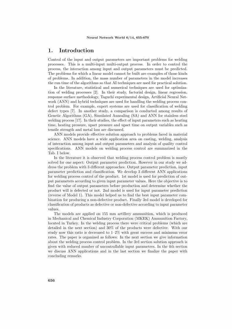
• In Model 1, we have 9 different input variables (x1 to x9) and 3 differentoutput variables (y1 to y3). In this model, there are 3 hidden layers with 10neurons in first hidden layer, 10 in second hidden layer and 5 neurons in thirdhidden layer.

• In Model 2, we have 3 input variables (y1 to y3) and 3 different outputvariables (x2, x3 and x5). In this model, there are also 3 hidden layers with10 neurons in first hidden layer, 10 in second hidden layer and 5 neurons inthird hidden layer.

• In Model 3, we have 9 different input variables (x1 to x9) and 3 differentoutput variables (y1 to y3). In this model, there is 1 hidden layer with 10neurons.

The generalized ANN architecture used in the models is shown in Fig. 4 below.We show the number of inputs as 1 to m, the number of neurons in hidden layersas 1 to ni and the number of outputs as 1 to o.

Fig. 4 Generalized ANN architecture.

4.2 MODEL 1. Output Parameter Prediction Model

In this model, values of 3 output variables (ZnR, FeR and CuR) are predictedaccording to given input variables. For this reason a BPNN model is used. Herethe aim is to find the values of output values before production and determinewhether the product will be defective or not. The best structure of network isfound by trial and error under several scenarios (by changing the number of hiddenlayers, neurons, type of transfer functions each layer etc.). The summary of trialand error results is given in Tab. IV. The output values can be predicted withapproximately 99% as seen in Tab. IV.

664


The network is trained with Levenberg–Marquardt Algorithm (LMA). LMA pro-vides a numerical solution to the problem of minimizing a function, generally non-linear, over a space of parameters of the function. These minimization problemsarise especially in least squares curve fitting and nonlinear programming [9]. Pri-mary application of LMA is in the least squares curve fitting problem: Given aset of m empirical datum pairs of independent and dependent variables, (xi, yi),optimize the parameters β of the model curve f(x, β), so that the sum of the squaresof the deviations becomes minimal as follows:

S(β) =m∑i=1

[yi − f(xi, β)]2

(3)

In order to measure the network performances Mean Squared Error (MSE) is usedas a performance measure. MSE is a network performance function. It measuresnetwork’s performance according to the mean of squared errors.

The MSE of a estimaton λ with respect to the estimated paramete θ is definedas follows:

MSE(λ) = E([λ− θ]2) (4)

For training Model 1, data are partitioned into 4. The training performance ofModel 1 is shown in Tab. V. For modeling ANN, MATLAB software is used [12].

4.3 MODEL 2. Input Parameter Prediction Model

In this model, values of 3 input variables (BDS, CTR and OSR), which are 3important classifiers, are predicted according to given output variables. For thisreason a reverse BPNN model is used.

Here the purpose is determining the values of most important input variablesaccording to given output values and finding best values for a defect-free product.For this model a 3× 10× 10× 5× 3 model structure is used. In this model, we use3 inputs which are ZnR, FeR and CuR. There are 3 hidden layers in the model.First hidden layer is composed of 10 neurons, second hidden layer is composed of10 neurons and third hidden layer is composed of 5 neurons. Model 2 is developedto find best values for 3 critical parameters which are BDS, CTR and OSR.

Here as a reverse application of 1st model, output variables are used as in-puts. Because we know the optimum values for output variables (which are pre-determined by Quality Control department) for a defect-free product, we use thenumerical values of outputs as input and try to predict the input values. Hereusing outputs and inputs in a reverse provided the advantage of finding best valuesof input variables for a defect-free product. This also enabled us to tackle theproblem with a different perspective. In the 1st model, we found the unknownvalues of output parameters for each product; However in Model 2, we use qualityspecification values of outputs (For a defect-free weld ZnR must be between 8–12%,FeR must be between 0.5–4% and CuR must be between 84–91.5%) as inputs.

For Model 2, a different structure from Model 1 is developed. The best structureis found by trial and error under several scenarios (by changing the number of

665


Number

Numberof

ofHidden

Activation

Functions

neuro

nsin

Itera

tion

MSE

rLayers

eac h

layer

Number

Value

Value

One

Sigmoid

11000

0.02399

0.490

Sigmoid

51000

0.00862

0.858

Sigmoid

10

1000

0.00420

0.934

Sigmoid

15

1000

0.00376

0.945

Sigmoid

15

1500

0.00376

0.945

HiperbolicTangent

15

1000

0.09997

0.836

Sigmoid

16

1000

0.00377

0.944

Sigmoid

20

1000

0.00718

0.903

Sigmoid

20+

1500

0.00718

0.903

Two

Sigmoid

(1)–Sigmoid

(2)

1–1

1000

0.01444

0.617

Sigmoid

(1)–Sigmoid

(2)

5–5

1000

0.01025

0.842

Sigmoid

(1)–Sigmoid

(2)

10–10

1000

0.00320

0.957

Sigmoid

(1)–HyperbolicTangen

t(2)

15–15

1000

0.01112

0.834

Sigmoid

(1)–Sigmoid

(2)

15–15

1000

0.00259

0.968

Sigmoid

(1)–Sigmoid

(2)

16–16

1000

0.00224

0.969

Sigmoid

(1)–Sigmoid

(2)

20–20

1000

0.00224

0.969

Sigmoid

(1)–Sigmoid

(2)

20+

–20+

1500

0.00224

0.969

Thr ee

Sigmoid

(1)–Sigmoid

(2)–Sigmoid

(3)

1–1–1

1000

0.01698

0.699

Sigmoid

(1)–Sigmoid

(2)–Sigmoid

(3)

5–5–5

1000

0.01321

0.747

Sigmoid

(1)–Sigmoid

(2)–Sigmoid

(3)

10–5–5

1000

0.00138

0.968

Sigmoid

(1)–Sigmoid

(2)–Sigmoid

(3)

10–5–5

1500

0.00138

0.968

Sigmoid

(1)–Sigmoid

(2)–Sigmoid

(3)

10–10–5

1000

0.00551

0.936

Sigmoid

(1)–HyperbolicTangent(2)–Sigmoid

(3)

10–10–5

1000

0.00111

0.969

Sigmoid

(1)–

HiperbolicTangent(2

)–Lin

ear(3

)10-1

0-5

1000

0.00002

0.999

Sigmoid

(1)–

HiperbolicTangent(2

)–Lin

ear(3

)10+–10+–5+

1500

0.00002

0.999

Tab.IV

Resultsoftrialanderrorforbest

ANN

architecture

forModel

1.

666


hidden layers, neurons, type of transfer functions at each layer etc.). The structuregiving minimum MSE in selected. The training performance of Model 2 is shownin Tab. V.

According to results of Model 2; OSR must 1155 mm/min, CTR value must beequal 77 mm and BDS value must be 6,65 m/min.

4.4 MODEL 3. Classification Model

Neural networks have proven themselves as proficient classifiers and are particularlywell suited for addressing non-linear problems. Given the non-linear nature of realworld phenomena, neural networks is certainly a good candidate for solving theproblem [4].

The classification model is built with 3 different approaches in this work. Firstapplication is carried out to determine which input parameter set results with adefective product and which ones with a defect-free product. In order to solve thisproblem three different BPNN models (Model 3.1: Feed forward backpropagationnetwork, Model 3.2: Cascade-forward backpropagation network and Model 3.3:feedforward backpropagation network with feedback from output to input) aredeveloped for classifying the products. In feed-forward backpropagation networks,the first layer has weights coming from the input. Each subsequent layer hasa weight coming from the previous layer. In cascade forward backpropagationnetworks, the first layer has weights coming from the input. Each subsequentlayer has weights coming from the input and all previous layers. In feed-forwardbackpropagation networks, with feedback from output to input, the first layer hasweights coming from the input. Each subsequent layer has a weight coming fromthe previous layer and there exists a feedback from output layer to inputs. For all3 models all layers have biases, the last layer is the network output.

ANN model architectures used in Model 3 are composed of an input layer, 1hidden layer and an output layer. There are 9 neurons (9 input parameters) ininput layer, 10 neurons in hidden layer, and 3 neurons (3 output parameters) inoutput layer (9×10×3). The best network architecture is found with trial and error.Several runs are conducted and the structure with minimum Mean Squared Error(MSE) is chosen. Performance of networks is discussed in “Results and Discussion”section. The outputs in ANN model are represented by unit vectors as: [1 1 1]= defective weld, [0 0 0] = defect-free weld. Each neuron in the output vectorrepresents a situation whether ZnR, FeR and CuR is between quality specificationsrespectively. Therefore [1 1 1] means that output quality specifications are not metand [0 0 0] means output quality specifications are met.

The network is trained with Levenberg–Marquardt Algorithm (LMA). For this“trainlm” learning function is used in the MATLAB software. “trainlm” is oftenthe fastest backpropagation algorithm and it is highly recommended as a first-choice supervised algorithm, although it does require more memory than otheralgorithms.

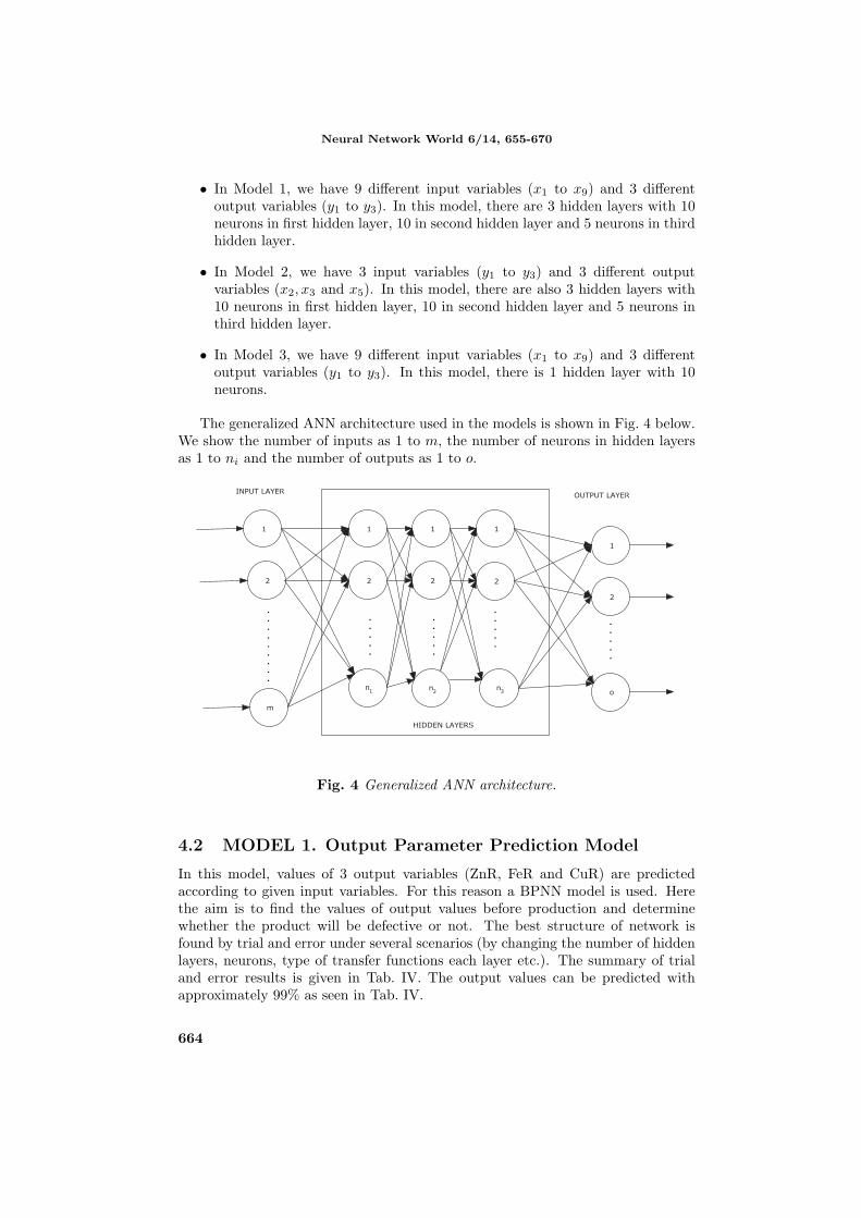
In Tab. V, training performances of Model 1, Model 2 and Model 3 are givenrespectively. Here epoch shows the number of iterations of neural network algo-rithm. Time shows total running time of algorithm in seconds in an Intel CoreDuo, 2.13 Ghz, 2 GB RAM desktop computer. MSE, which is a common measure

667


of performance, shows the mean squared error of training performance (explainedin Section 4.2). SSE shows the sum of squared error of training performance. Withcorrelation coefficient (r) we have information about the training of network. Ittakes values between −1 and 1. If r is close to 1, it shows success rate of thelearning.

Performance criteria fortraining performance of Model 1* Model 2 Model 3Model 1, 2 and 3 3.1 3.2 3.31. Epoch 50 100 32 100 182. Time (seconds) 28 52 34 65 10

3. TrainingPerformance

MeanSquaredError(MSE)

1,56*10−6 8,99*10−3 2,02*10−18 2,95*10−12 5,87*10−21

Sum ofSquaredErrors(SSE)

3,1*10−4 1,8*10−2 4*10*10−16 6*10−10 1,2*10−20

4. Correlation coeff. (r) 0,99 0,95 0,99 0,99 0,99

*4 different models (by choosing different parts of data for training and test) are developed for

Model 1. Best performance results among 4 different models are shown in the table for Model 1.

Tab. V Training performance of Models 1, 2 and 3.

5. Results and Discussion

This paper presents results of the research on development of a new approach basedon 3 different ANN models to predict best input-output parameter combination andto classify products. In this new modeling approach, prediction and classificationcapabilities of ANNs are used together with input-output interactions for devel-oping a defect-free welding operation. Another innovation point in the study is areverse application of ANN method as shown in the 2nd model. In the ANN mod-els, the training and testing results have shown a strong potential for predictionof best parameter interactions. It is discovered that a high level of performance isaccomplished by all the methods used in this study. In virtue of this study, thereproduction, salvage, scrap and retrieval costs for 155mm artillery ammunitionare minimized.

Model 1 is used for output parameter prediction and a model with 99% successrate is created; Model 2 is used for input prediction as a reverse ANN applicationand values of 3 important input parameters are found; Model 3 is used for classi-fication of defective and defect-free products and a classification model with 95%success rate is found. For all of the models, welding operation data of 200 am-munitions are used for prediction and classification analysis. %75 of the data areused for training of the networks. Remaining 25% are used for testing the networkperformance.

The main quality indicator of a neural network is to predict accurately theoutput of unseen test data. In this study, we have benefited from classification and

668


prediction success of BPNNs. The classification and prediction performance resultsshow the advantages of Backpropagation neural networks: it is rapid, noninvasiveand inexpensive. Another advantage of the models is, with any input parametercombination, we can execute the model and find the output values in a few seconds.

In addition, BPNN does not explain the classification results by rules. In orderto create rules from ANN results, intelligent classification algorithms can be inte-grated to ANN codes. And the final algorithm can find best classifiers, which isconsidered as a future study.

Acknowledgement

This study was financially supported by a grant from Republic of Turkey Ministryof Science, Industry and Technology with Grant No.: 00748.STZ.2010-2.

References

[1] ATES H. Prediction of gas metal arc welding parameters based on artificial neural networks.Materials and Design. 2007, 28(7), pp. 2015–2023, doi: 10.1016/j.matdes.2006.06.013.

[2] BENYOUNIS K.Y., OLABI A.G. Optimization of different welding processes using statisticaland numerical approaches – A reference guide. Advances in Engineering Software. 2008,39(6), pp. 483–496, doi: 10.1016/j.advengsoft.2007.03.012.

[3] FAUSETT L. Fundamentals of neural Networks, architectures, algorithms and applications.Prentice Hall, 1994.

[4] KHASHEI M., BIJARI M. An artificial neural network model (p, d, q) for timeseries fore-casting. Expert Systems with Applications. 2010, 37(1), pp. 479-489, doi: 10.1016/j.eswa.2009.05.044.

[5] KIM S., et al. Optimal design of neural networks for control in robotic arc welding. Roboticsand Computer-Integrated Manufacturing. 2004, 20(1), pp. 57–63, doi: 10.1016/S0736-5845(03)00068-1.

[6] LI C., et al. Cryptanalysis of a chaotic neural network based multimedia encryption scheme.In: In: AIZAWA, et al., eds. Proceedings of the 5th Pacific Rim Conference on Multimedia,Advances in Multimedia Information Processing - PCM 2004, Part III, Lecture Notes inComputer Science, Tokyo, Japan. Springer-Verlag, 2005, 3333, pp. 418-425.

[7] LIAO T.W. Classification of welding flaw types with fuzzy expert systems. Expert Systemswith Applications. 2003, 25(1), pp. 101–111, doi: 10.1016/S0957-4174(03)00010-1.

[8] LUO H., et al. Application of artificial neural network in laser welding defect diag-nosis. Journal of Materials Processing Technology. 2005(1-2), 170, pp. 403–411, doi:10.1016/j.jmatprotec.2005.06.008.

[9] MARQUARDT D. An algorithm for least-squares estimation of nonlinear parameters. SIAMJournal on Applied Mathematics. 1963, 11(2), pp. 431–441, doi: 10.1137/0111030.

[10] MARTIN O., LOPEZ M., MARTIN F. Artificial neural networks for quality control byultrasonic testing in resistance spot welding. Journal of Materials Processing Technology.2007, 183(2-3), pp. 226–233, doi: 10.1016/j.jmatprotec.2006.10.011.

[11] MARTIN O., TIEDRA D.P., LOPEZ M. Artificial neural networks for pitting potentialprediction of resistance spot welding joints of AISI 304 austenitic stainless steel. CorrosionScience. 2010, 52(7), pp. 2397–2402, doi: 10.1016/j.corsci.2010.03.013.

[12] MATHWORKS FOUNDATION MATLAB. Matlab R2009a. [software]. 2009-06-01 [ac-cessed 2012-01-01]. Available from: http://www.mathworks.com/products/neural-network/.

[13] MIRAPEIX J., et al. Real-time arc-welding defect detection and classification with principalcomponent analysis and artificial neural networks. NDT&E International. 2007, 40(4), pp.315–323, doi: 10.1016/j.ndteint.2006.12.001.

669


[14] NANCY R. T. The Quality Toolbox. 2nd ed. USA: ASQ Quality Press, 2005.

[15] PAL S., PAL K. S., SAMANTARAY K. Artificial neural network modeling ofweld joint strength prediction of a pulsed metal inert gas welding process usingarc signals. Journal of materials processing technology. 2008, 202(1-3), pp. 464–474,doi:10.1016/j.jmatprotec.2007.09.039.

[16] RUSSELL S., NORVIG P. Artificial Intelligence: A Modern Approach. 2nd. ed., PrenticeHall, 2002.

[17] SATHIYA P., et al. Optimization of friction welding parameters using evolutionary computa-tional techniques. Journal of Materials Processing Technology. 2009, 209(5), pp. 2576–2584,doi: 10.1016/j.jmatprotec.2008.06.030.

[18] SHIHAB K. A backpropagation neural network for computer network security. Journal ofComputer Science. 2006, 2(9), pp. 710-715, doi: 10.3844/jcssp.2006.710.715.

[19] TAY K.M., BUTLER C. Modeling and Optimizing of a Mig Welding Process-A Case StudyUsing Experimental Designs and Neural Networks. Quality and Reliability Engineering In-ternational. 1997, 13(2), pp. 61–70, doi: 10.1002/(SICI)1099-1638(199703)13:2<61::AID-QRE69>3.0.CO;2-Y.

[20] OZERDEM M.S., SEDAT K. Artificial neural network approach to predict the mechanicalproperties of Cu–Sn–Pb–Zn–Ni cast alloys. Materials and Design. 2009, 30(3), pp. 764–769,doi: 10.1016/j.matdes.2008.05.019.

[21] YE N., VILBERT S., QIANG C. Computer intrusion detection through EWMA for autocorrelated and uncorrelated data. IEEE Trans. Reliability. 2003, 52(1), pp. 75-82, doi:10.1109/TR.2002.805796.

670

Documents

WELDING PROCESS OPTIMIZATION WITH ARTIFICIAL NEURAL ... · PDF fileWELDING PROCESS OPTIMIZATION WITH ARTIFICIAL NEURAL NETWORK ... paper presents a new modeling approach on prediction