Welfare Implications in Intermediary Networks

Thanh Nguyen∗ Karthik Kannan†

May 2020

Abstract

We study the welfare implications of competing middlemen in a two-sided market, wheregoods are intermediated between providers and purchasers. In our model, each intermediary setsthe quantities it intermediates, and the prices are a consequence of a Cournot competition. Ouranalysis shows that, unlike traditional markets, increasing competition is not always beneficialfor market efficiency and that mergers can have an ambiguous effect on efficiency. We alsoanalyze how the underlying network influences social welfare. We define parameter wG as theintermediary capacity of the network G and show that the price of anarchy is at least 1− 1

2wG+1 .These results suggest an intuitive and simple measure for the level of competitiveness in anetworked market involving intermediaries.

1 Introduction

Because of digital technologies, platform markets – where an intermediary enables connections

between providers and purchasers of services – are becoming popular. In addition to the new-age

companies (such as Uber, Google, and Facebook), many leading ‘traditional’ companies, including

Cummins, Kaiser Permanente, GE, are developing their digital platform strategies. They perceive

the push toward a platform business model as being critical to their survival (Accenture, 2016).

So, an extensive and growing literature is now focused on developing platform strategies from

a single firm’s perspective. However, very few prior works study the implications of platforms

in a competitive environment. Understanding the eco-systems of competing and heterogeneous

platforms is important because it provides insights for not only individual companies but also the

policymakers. For example, when discussing the platform markets, Assistant Attorney General

Makan Delrahim said, “. . . we, as antitrust enforcers, need to pay close attention to competitive

∗Krannert School of Management, Purdue University, email: nguye161@purdue.edu†Krannert School of Management, Purdue University, email: kkarthik@purdue.edu

1

constraints, to first make sure we don’t enforce away pro-competitive business models, but also to

be vigilant that conduct does not unreasonably constrain the ability of new competitors to compete

on the merits.” The nature of competition in the platform markets is evolving. We first started to

think about this research question because of the following anecdote.

In 2008, Google and Yahoo proposed a joint partnership that would have allowed Yahoo to use

Google’s ad service to intermediate and deliver ads for Yahoo as well as its partners’ sites in the

U.S. and Canada. The benefits of this agreement were mentioned in Drummond (2008):

“We feel that the agreement would have been good for publishers, advertisers, andusers – as well, of course, for Yahoo! and Google. Why? Because it would have allowedYahoo! (and its existing publisher partners) to show more relevant ads for queries thatcurrently generate few or no advertisements. Better ads are more useful for users, moreefficient for advertisers, and more valuable for publishers.”

However, the agreement never materialized because of antitrust concerns:

“After four months of review, including discussions of various possible changes to theagreement, it’s clear that government regulators and some advertisers continue to haveconcerns about the agreement. Pressing ahead risked not only a protracted legal battlebut also damage to relationships with valued partners. . . [S]o, we have decided to endthe agreement.”

Since then, this market has undergone significant changes. Mergers are quite commonplace:

Microsoft bought aQuantitative in 2012, and Yahoo purchased Interclick in 2011. Such mergers

are not limited to advertising markets. The ride-sharing market is also undergoing a significant

transformation. In that sector, Lyft and Didi Chuxing were initially in a partnership to thwart

Uber. Eventually, Uber merged its operation with Didi Chuxing. Yet another example is in the

e-commerce space, where online market-makers are intermediaries connecting sellers and buyers.

Amazon and Walmart competed fiercely to buy the Indian online retailer Flipkart, which Walmart

eventually won. The issues we study in our paper are not just specific to the new age markets

but also are relevant to other markets with similar intermediated structures. The network services

2

segment is evolving with “intermediaries” such as AT&T acquiring other intermediaries such as

DirectTV. Similarly, retailers may be viewed as simply intermediating between manufacturers and

consumers. Our analysis provides insights into such cases also. For example in such an intermedi-

ated ecosystem, we show that there are sources of inefficiency raised by intermediaries and networks

that don’t exist in traditional models. Given our generic focus, our model is set up to be agnostic

to contexts. The examples provided throughout the paper are meant to help a reader connect

different entities in our model to reality.

An oft-cited rationale against this kind of proposed agreement has been that mergers and coali-

tions among firms increase the monopoly power, and harms both consumer surplus and social

welfare. While this rationale may be appropriate in traditional markets involving only one type of

customer, such an analysis does not always extend to two-sided markets. Even Supreme Court is

open to considering such alternatives: “We have therefore felt relatively free to revise our legal anal-

ysis as economic understanding evolves and . . . to reverse antitrust precedents that misperceived

a practice’s competitive consequences.” Such mergers or even agreements may allow participants

(say, buyers, advertisers, or passengers) on one side to access participants on the other (correspond-

ingly, sellers, publishers, or drivers). By opening up access to the other market, the coalition may

facilitate more transactions between the two sides, improving social welfare as a whole. To illustrate

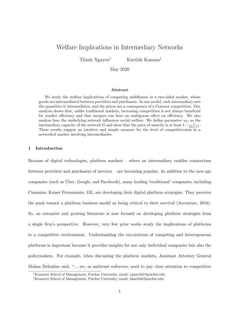
the complexity of the intermediary networks, consider the highly stylized network structure in the

two scenarios shown in Figure 1.

In scenario I, three intermediaries A, B, and C, are competing to deliver a service for purchasers

3 and 4 by providers 1 and 2. In scenario II, A and B merge. Trade-offs need to be considered

because of the mergers. Notice that in Scenario I, A and B compete to deliver service by 1 to 4; but

C is the only intermediary between 2 and 3. On the other hand, when A and B merge, the merged

firm AB becomes a monopoly when serving 1 and 4; however, the merged entity now competes with

3

A

C

B

1

2

3

4

A-B

C1

2

3

4

I: Three intermediary network II: Merging of A and B

Figure 1: Two different networks: before and after merging of A and B.

C to deliver service for purchaser 3 by provider 2. Thus, unlike the traditional seller-buyer models,

the merging of intermediaries can even increase competition. As a result, the overall efficiency of

such an economy depends critically on the underlying network structure. This means that, in large

and complex networks, understanding the implications of antitrust policies becomes difficult. In

this paper, we present this idea more formally. Besides, we ask the following question. Can we use

a simple but intuitive set of network parameters to estimate the level of efficiency? The answers

to this question not only give insights into the nature of competition among the intermediaries

in a networked market but also provide guidelines for conducting policy analysis when comparing

alternate network structures. As platform-based markets continue to grow, one can anticipate

more partnerships, mergers, and acquisitions. Hence, understanding the welfare implications of

these markets is becoming increasingly important.

We investigate the welfare implications of a marketplace involving multiple intermediaries.

An intermediary may serve multiple providers (e.g., web publishers with ad-slots, or ride-sharing

drivers) and purchasers (e.g., advertisers, ride-sharing passengers respectively). A provider or a

purchaser may connect with multiple intermediaries. The dependencies create a networked market

structure. We study how the nature of the networked structure has welfare implications.

For the study, we formulate the problem initially as a 3-partite graph with the edges cor-

responding to the networked structure. This structure is reduced to a bipartite graph by making

4

assumptions. In the real markets, the price clearing mechanisms generally vary – for example, Gen-

eralized Second Price (GSP) is used in the ad auctions or dynamic ‘surge prices’ for ride-shares,

etc. We employ a Cournot competition model as the price clearing mechanism. As we will expand

later, Cournot has been used in prior works to effectively capture competition – the competition

amongst the providers themselves and purchasers themselves. Such a model was also used exten-

sively when studying welfare implications in traditional markets. With that pricing mechanism,

when the intermediaries act optimally, the problem can be reduced to a single convex program, the

solution of which corresponds to the decisions of the individual intermediaries at equilibrium. A

key feature of the resulting quadratic program is that it allows us to identify a unique equilibrium.

Thus, the problem is amenable to some robust comparative static analysis.

With the convex program, we provide several comparative analyses. We show that competition

in an unbalanced market can reduce social welfare. Mergers in sparse markets, however, can create

competition and improve market efficiency. This is a seemingly counter-intuitive result different

from the results in traditional markets. We also study how well the best social welfare obtained

using the networked structure in equilibrium compares with the maximum social welfare by using

the price of anarchy. The price of anarchy is dependent on the intensity of competition, which we

capture through a measure we call the intermediary capacity of the network. Specifically, we find

that the larger the intermediary capacity of the network, the more efficient the equilibrium.

The rest of the paper is organized as follows. In the following section, we survey the related

literature. Section 3 formally defines the model, which is analyzed in Section 4. Section 5 provides

new insights about how competition and mergers influence welfare. Section 6 studies the impact

of the network structure on the level of efficiency. Section 8 concludes the paper.

5

2 Literature Review

Our work relates to several streams of research. The first stream is the well-established literature on

platform-based markets. The second stream is the literature on networked markets that is nascent

but growing extensively. We provide a brief survey of the first stream and a somewhat more

extended one of the second. Since there is some related work in individual contexts (ad markets,

ride-sharing, etc.) we also provide a brief survey of the related work as the third subsection.

2.1 Platform Economics

Our paper studies intermediaries that connect different sides of a market as found in the literature

on network-effect based platforms. This domain has been extensively researched. The early focus

on this literature was on single-sided networks (e.g., the seminal work by Katz and Shapiro, 1985)

but has expanded in recent years to include multi-sided platforms (e.g., Parker and Van-Alstyne,

2005, study two-sided networks). Many papers have analyzed the strategic aspects of managing

these network-based platforms. For example, they analyze what the pricing strategies should be

how to launch a network effects based market.

A few recent papers have also studied welfare implications. Lee (2014) has studied the problems

involving single-sided networks. Others (Evans and Schmalensee, 2013; Weyl, 2010) have studied

it with respect to the two-sided markets. To the best of our knowledge, these papers have not

considered the welfare implications of mergers across the intermediaries. Moreover, the “network”

effects studied in these papers are very different from ours. In particular, most papers in platform

economic literature model symmetric environments and focus on the externality/complementarity

effect that a platform creates for its members. This is, for example, integrated directly into a

member’s utility that depends on how many others are using the same platform. Our paper, on the

other hand, moves away from such effects to focus on the impact of heterogeneity in the connection

6

structure. This other type of “network effect” is actively investigated by a relatively new but

fast-growing literature on network markets that we survey next.

2.2 Network Markets

Most of the early literature on network markets focuses on seller-buyer networks. Kranton and

Minehart (2001), Corominas-Bosch (2004), (Abreu and Manea, 2012; Manea, 2011; Polanski, 2007)

and Elliott (2014) are a few examples. By assumption, all these papers rule out intermediaries and

focus only on the trade between buyers and sellers.

Blume et al. (2009) was among the first to investigate a mediated market in a network setting.

The network structure in our paper is similar to that of Blume et al. (2009). However, Blume

et al. (2009) consider Bertrand competition among intermediaries and assume buyers have unit

demand. In two-sided markets, such as ad-networks, considering multi-unit demand and supply

with heterogeneity among the players is more relevant. In the context of ad-intermediaries, agents

target different amounts of impressions, and trades are executed by market-clearing auctions. It

is natural, therefore, to study such a network using a Cournot model, which we do in this paper.

Such a characterization is a unique feature of our model. Because of the differences in the model

characterizations, the equilibrium outcomes are also different. All equilibria in Blume et al. (2009)

are efficient, whereas, that is not the case in our model. Hence, our main aim of measuring the

level of efficiency based on the structure of the underlying network is relevant.

Our paper is closely related to recent models of Cournot competition in networks by Bimpikis

et al. (2018) and Perakis and Sun (2014). However, unlike us, they do not consider intermediaries.

On the contrary, we show in Section 5 new insights on how competition and mergers of intermedi-

aries influence welfare. These effects are absent in models without intermediaries such as Bimpikis

et al. (2018) and Perakis and Sun (2014). For example, Bimpikis et al. (2018) studies mergers of

firms in two-sided market. The effect on welfare for that type of mergers is different from our paper.

7

The mathematics behind them are also different. Our paper shows that the unique equilibrium can

characterized by a convex program.1 Note that with network games, for a general class of utilities,

it is quite hard to prove the existence of equilibrium, let alone proving uniqueness. For example,

in Bimpikis et al. (2018), they need additional assumptions such as positive trade occurring in all

links for the comparative analysis.

Our model formulation employs a model of Cournot competition. Bose et al. (2014) also studies

intermediaries and market makers in a Cournot game. The main question that Bose et al. (2014)

addresses is how to modify the objective of market makers to maximize social welfare. Here, we

focus on how the network structure influences efficiency.

Several recent papers have studied intermediaries, including Nguyen (2015b, 2017) and Manea

(2018). The settings in these papers, however, are quite different from ours. In particular, they

study the incentive of non-cooperative bargaining and assume unit-demand agents. Even though

in the advertising industry, bargaining is part of the contracts, automated auctions control the

majority of the interaction among the agents in those studies. Feldman et al. (2010) study the

equilibrium properties in a model where buyers buy ad slots from a central buyer via a set of

competing intermediaries. They demonstrate how the interaction between the auction design and

double marginalization affects outcomes. Our paper differs from this work in that intermediaries

in our model connect between multiple buyers and sellers, and in that the prices are determined

by the Cournot (sub)markets.

2.3 Context Specific Literature

Digital and search ads have received significant attention from various disciplines, including com-

puter science, marketing, information systems, and economics. A seminal piece in this regard is

1Characterizing equilibrium with convex programming technique is not new, for example in bargaining networkgamesNguyen (2015a), in combinatorial auction Bikhchandani and Ostroy (2002). However, we are not aware of thesame technique being used in this specific context and such a formulation allows us to conduct comparative analysiseasily.

8

by Edelman et al. (2007), who analyzes the equilibrium of the GSP auction. Variants of GSP

have been implemented and also studied. Feng et al. (2007) using simulations and Balachander

et al. (2009) using game-theory compare alternative GSP auction policies. More generally, papers

have also evaluated the welfare implications of the search ads market. Usually, they are executed

in the context of a single ad-intermediary. For example, Chen and He (2011) evaluated the effi-

ciency of ads on the consumer search process. Similarly, welfare implications are also studied when

considering policy changes for the auctions. As another example, Shin (2015) study the subject

of search engines requiring budget constraints for advertisers in GSP auctions. More generally,

computer science has extensively studied mechanism design problems in the ad network context.

One stream within this literature employs matching algorithms – specifically, how to match ads to

positions (e.g., Mehta et al., 2007; Caragiannis et al., 2015). Note that we focus on multiple search

ad intermediaries.

The literature on ride-sharing has been expanding rapidly in recent years. See for example

Cachon et al. (2017); Bimpikis et al. (ming); Banerjee et al. (2017); Fang et al. (2017). The

focus of this literature, however, has been on the optimal design of a monopoly’s matching and

pricing mechanisms. Our paper, on the other hand, considers the problem from an industry level

perspective. Given that there are many competing platforms and the connections of these platforms

with the two sides of the markets are heterogeneous, our paper analyzes the impact of such an

underlying network structure on the efficiency of the whole ecosystem.

3 The Model

Many intermediated markets are highly dynamic and the demand and supply of quantities are

often ephemeral. It is often quite hard to capture the changing aspects of a model. Given our

focus on studying welfare implications, for the sake of tractability, we study a single-period game

using a stylized static competitive model. Let G be an exogenous tripartite network involving I

9

IntermediariesProviders Purchasers

IJ K

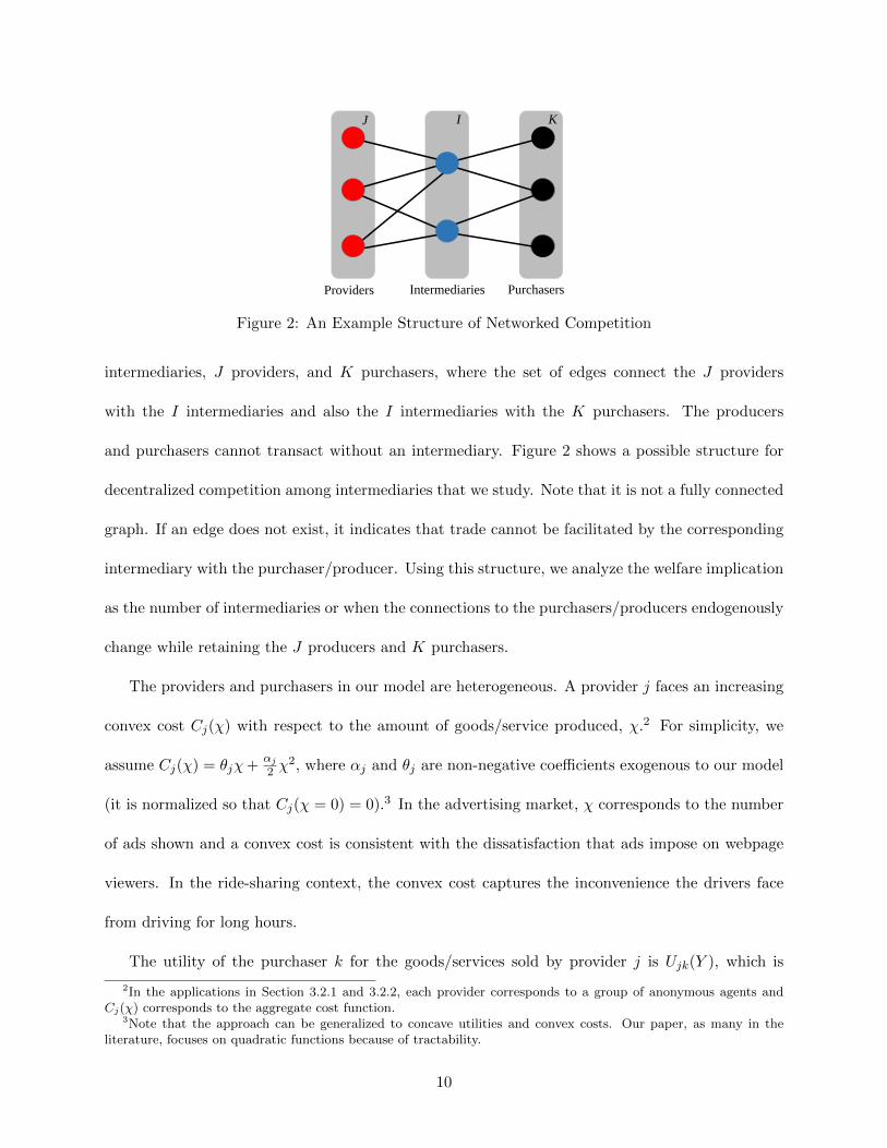
Figure 2: An Example Structure of Networked Competition

intermediaries, J providers, and K purchasers, where the set of edges connect the J providers

with the I intermediaries and also the I intermediaries with the K purchasers. The producers

and purchasers cannot transact without an intermediary. Figure 2 shows a possible structure for

decentralized competition among intermediaries that we study. Note that it is not a fully connected

graph. If an edge does not exist, it indicates that trade cannot be facilitated by the corresponding

intermediary with the purchaser/producer. Using this structure, we analyze the welfare implication

as the number of intermediaries or when the connections to the purchasers/producers endogenously

change while retaining the J producers and K purchasers.

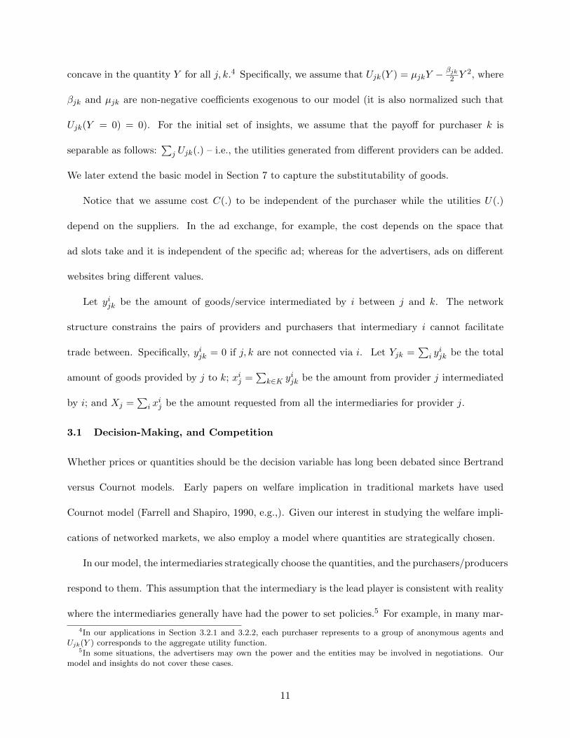
The providers and purchasers in our model are heterogeneous. A provider j faces an increasing

convex cost Cj(χ) with respect to the amount of goods/service produced, χ.2 For simplicity, we

assume Cj(χ) = θjχ+αj2 χ

2, where αj and θj are non-negative coefficients exogenous to our model

(it is normalized so that Cj(χ = 0) = 0).3 In the advertising market, χ corresponds to the number

of ads shown and a convex cost is consistent with the dissatisfaction that ads impose on webpage

viewers. In the ride-sharing context, the convex cost captures the inconvenience the drivers face

from driving for long hours.

The utility of the purchaser k for the goods/services sold by provider j is Ujk(Y ), which is

2In the applications in Section 3.2.1 and 3.2.2, each provider corresponds to a group of anonymous agents andCj(χ) corresponds to the aggregate cost function.

3Note that the approach can be generalized to concave utilities and convex costs. Our paper, as many in theliterature, focuses on quadratic functions because of tractability.

10

concave in the quantity Y for all j, k.4 Specifically, we assume that Ujk(Y ) = µjkY −βjk2 Y

2, where

βjk and µjk are non-negative coefficients exogenous to our model (it is also normalized such that

Ujk(Y = 0) = 0). For the initial set of insights, we assume that the payoff for purchaser k is

separable as follows:∑

j Ujk(.) – i.e., the utilities generated from different providers can be added.

We later extend the basic model in Section 7 to capture the substitutability of goods.

Notice that we assume cost C(.) to be independent of the purchaser while the utilities U(.)

depend on the suppliers. In the ad exchange, for example, the cost depends on the space that

ad slots take and it is independent of the specific ad; whereas for the advertisers, ads on different

websites bring different values.

Let yijk be the amount of goods/service intermediated by i between j and k. The network

structure constrains the pairs of providers and purchasers that intermediary i cannot facilitate

trade between. Specifically, yijk = 0 if j, k are not connected via i. Let Yjk =∑

i yijk be the total

amount of goods provided by j to k; xij =∑

k∈K yijk be the amount from provider j intermediated

by i; and Xj =∑

i xij be the amount requested from all the intermediaries for provider j.

3.1 Decision-Making, and Competition

Whether prices or quantities should be the decision variable has long been debated since Bertrand

versus Cournot models. Early papers on welfare implication in traditional markets have used

Cournot model (Farrell and Shapiro, 1990, e.g.,). Given our interest in studying the welfare impli-

cations of networked markets, we also employ a model where quantities are strategically chosen.

In our model, the intermediaries strategically choose the quantities, and the purchasers/producers

respond to them. This assumption that the intermediary is the lead player is consistent with reality

where the intermediaries generally have had the power to set policies.5 For example, in many mar-

4In our applications in Section 3.2.1 and 3.2.2, each purchaser represents to a group of anonymous agents andUjk(Y ) corresponds to the aggregate utility function.

5In some situations, the advertisers may own the power and the entities may be involved in negotiations. Ourmodel and insights do not cover these cases.

11

kets, the intermediaries choose the market-clearing (or price-determining) mechanisms: be it GSP

for ad auctions or surge prices for ride-sharing context. Another way to note the power position

is to compare the number of providers or purchasers versus the intermediaries. Since typically

the fewer number of intermediaries (e.g., Google, Uber, Lyft) exist, it is reasonable to assume the

intermediaries hold power.6 Next, we describe how our setup is framed as a Cournot model.

Before we describe our model, note the following key features about a standard Cournot model:

• The demand curve assumed in the standard Cournot model is nothing more than the marginal

benefit curve of the entire set of customers. The marginal benefit curve is simply the aggrega-

tion of the marginal utility curves of individual consumers with no assumption on how many

consumers generate the aggregate utility. Therefore, independent on whether it is single or

multiple consumers, the demand function is the marginal benefit curve.

• Given an aggregate x chosen by the firm and the aggregate utility U(.), the market clearing

price is the price that maximizes U(x) − p · x when the aggregate consumption of all the

customers is x. This explains why the market-clearing price is equal to the marginal benefit

curve and also that demand equals supply.

• In a standard Cournot, the market clearing price is obtained from a multi-unit uniform-

price auction when the number of units auctioned equal the aggregate quantities set by

the firms. The market-clearing price as the inverse demand function can be implemented

with minimal requirements on knowledge of private information. So, we assume that the

firm(s) are aware of the market-clearing price. Prior work has used this approach for various

economic environments. For example, Milgrom (2004) argues that, in a model with positive

supply elasticity, the “auction outcomes resemble a Cournot competition among buyers” when

6These companies do not have limitless power. In some cases, governments have intervened to limit the surgeprices. For our analysis, as we mentioned earlier, we construct a stylized parsimonious model for our analysis.

12

modeling the FCC spectrum auctions. Vasin and Kartunova (2016) studies the electricity

markets using a similar structure. Even in ad-auctions, Ashlagi et al. (2018); Nava (2015)

and Bimpikis et al. (2018) employ Cournot models for their analyses. Daughtery (2008)

provides a survey of such works that have used Cournot models. A work cited in their survey

is Klemperer (1986) who shows the conditions when their modeling of a competition resembles

Cournot outcomes.

• The Cournot model is laid out in a purchasing or procuring setting. (1) The firms may supply

a quantity of goods to sell to purchasers/consumers; or (2) the firms may procure a certain

quantity from providers/sellers. The bullet points so far have focused on the latter setting.

Our model combines both the producer- and purchaser-markets, with intermediaries as the

lead player in both and also intermediating between the two. Our information structure is no

different from the standard Cournot: the intermediaries are aware of the market-clearing price,

which corresponds to the marginal benefit (equivalently, supply) function that is independent of the

number of purchasers (equiv., producers) generating the aggregate utility (equiv., supply). In this

regard, as Footnotes 2 and 4 mention, the purchasers and producers could themselves correspond

to multiple agents. We additionally assume that, in our network, the intermediaries do not even

need to know the network structure but only their connections.

The equilibrium of our Cournot model may be viewed as the convergence of a tatonnement

process. The intermediaries can adjust their quantities if they can improve their payoff. At each

step of this adjustment process, they do so by changing these quantities by a small amount to

test price elasticity and to observe if these are indeed profit improving. Each step of this process

requires little private information and thus naturally reflects the dynamic of a real market.

For all these reasons, the Cournot approach models the essential elements of a complex market.

To be tractable, it necessarily abstracts away from details, such as bargaining and optimal contract

13

design. Our paper, therefore, uses this approach as a natural model to study the effects of network

structure on competition and welfare of the market.

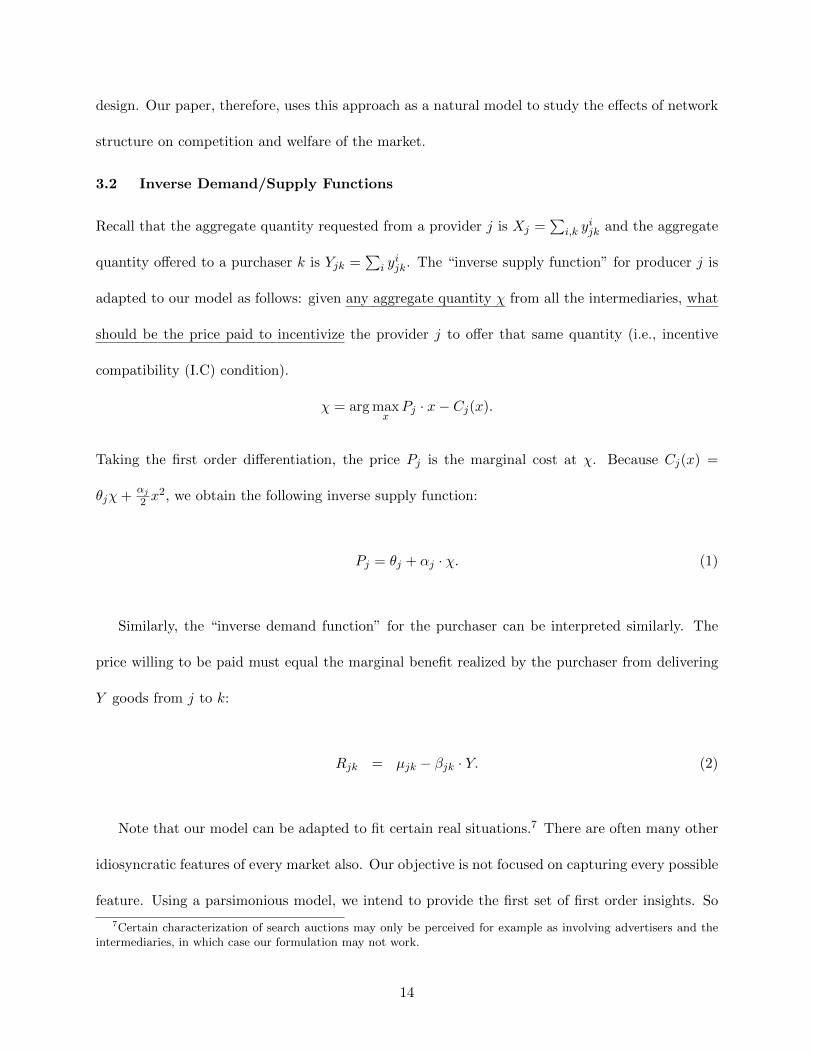
3.2 Inverse Demand/Supply Functions

Recall that the aggregate quantity requested from a provider j is Xj =∑

i,k yijk and the aggregate

quantity offered to a purchaser k is Yjk =∑

i yijk. The “inverse supply function” for producer j is

adapted to our model as follows: given any aggregate quantity χ from all the intermediaries, what

should be the price paid to incentivize the provider j to offer that same quantity (i.e., incentive

compatibility (I.C) condition).

χ = arg maxx

Pj · x− Cj(x).

Taking the first order differentiation, the price Pj is the marginal cost at χ. Because Cj(x) =

θjχ+αj2 x

2, we obtain the following inverse supply function:

Pj = θj + αj · χ. (1)

Similarly, the “inverse demand function” for the purchaser can be interpreted similarly. The

price willing to be paid must equal the marginal benefit realized by the purchaser from delivering

Y goods from j to k:

Rjk = µjk − βjk · Y. (2)

Note that our model can be adapted to fit certain real situations.7 There are often many other

idiosyncratic features of every market also. Our objective is not focused on capturing every possible

feature. Using a parsimonious model, we intend to provide the first set of first order insights. So

7Certain characterization of search auctions may only be perceived for example as involving advertisers and theintermediaries, in which case our formulation may not work.

14

long as the tensions associated with those insights exist, the welfare outcomes will be similar.

With this mind, we provide in the following subsection interpretations of the model and “inverse

supply/demand functions” in two settings: ad-exchange networks and ride-sharing platforms.

3.2.1 Ad-Exchange

An ad-exchange may be a large market and we can view each provider j as a group of publishers

having similar types of adpositions – e.g., possible ad positions across the sports sections of various

online magazines. We call this a buying sub-market j. Similarly, each purchaser k can be thought

of as a group of advertisers with similar characteristics – sellers of sneakers and gym-equipment.

We call this a selling sub-market k. Intermediaries buy ad-quantities from publishers and sell them

to advertisers. Then, yijk is the amount of trade transacted between j and k via intermediary i.

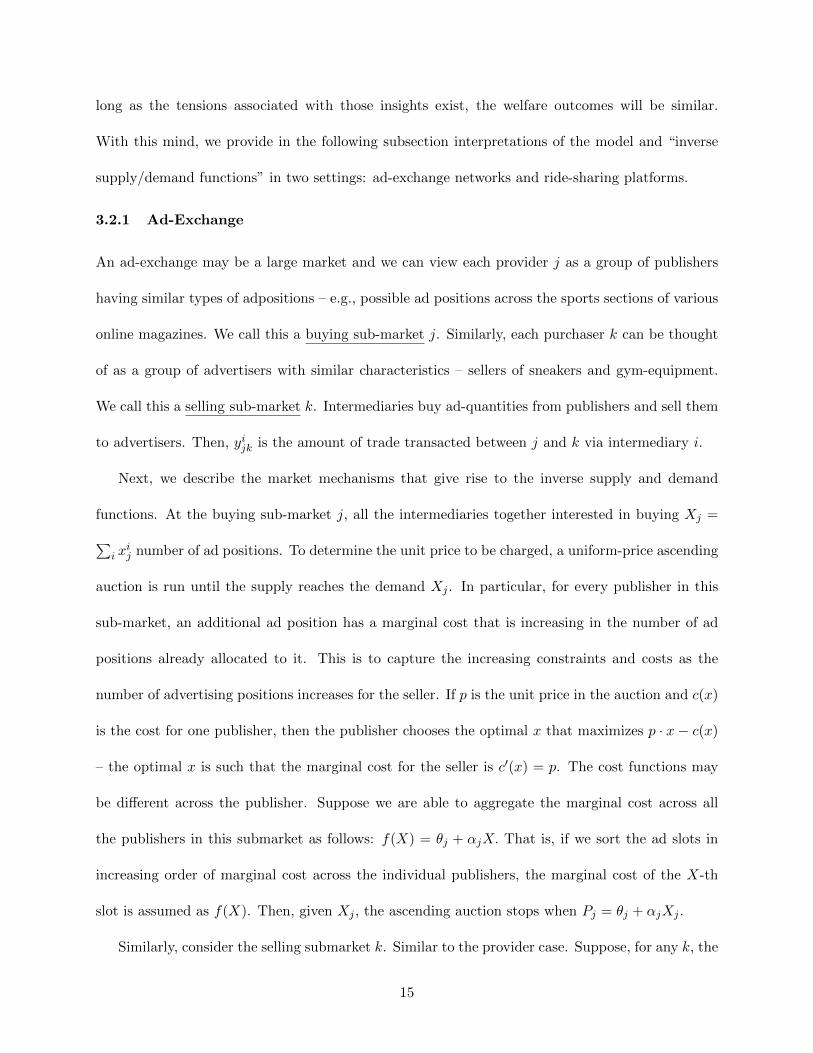
Next, we describe the market mechanisms that give rise to the inverse supply and demand

functions. At the buying sub-market j, all the intermediaries together interested in buying Xj =∑i x

ij number of ad positions. To determine the unit price to be charged, a uniform-price ascending

auction is run until the supply reaches the demand Xj . In particular, for every publisher in this

sub-market, an additional ad position has a marginal cost that is increasing in the number of ad

positions already allocated to it. This is to capture the increasing constraints and costs as the

number of advertising positions increases for the seller. If p is the unit price in the auction and c(x)

is the cost for one publisher, then the publisher chooses the optimal x that maximizes p · x− c(x)

– the optimal x is such that the marginal cost for the seller is c′(x) = p. The cost functions may

be different across the publisher. Suppose we are able to aggregate the marginal cost across all

the publishers in this submarket as follows: f(X) = θj + αjX. That is, if we sort the ad slots in

increasing order of marginal cost across the individual publishers, the marginal cost of the X-th

slot is assumed as f(X). Then, given Xj , the ascending auction stops when Pj = θj + αjXj .

Similarly, consider the selling submarket k. Similar to the provider case. Suppose, for any k, the

15

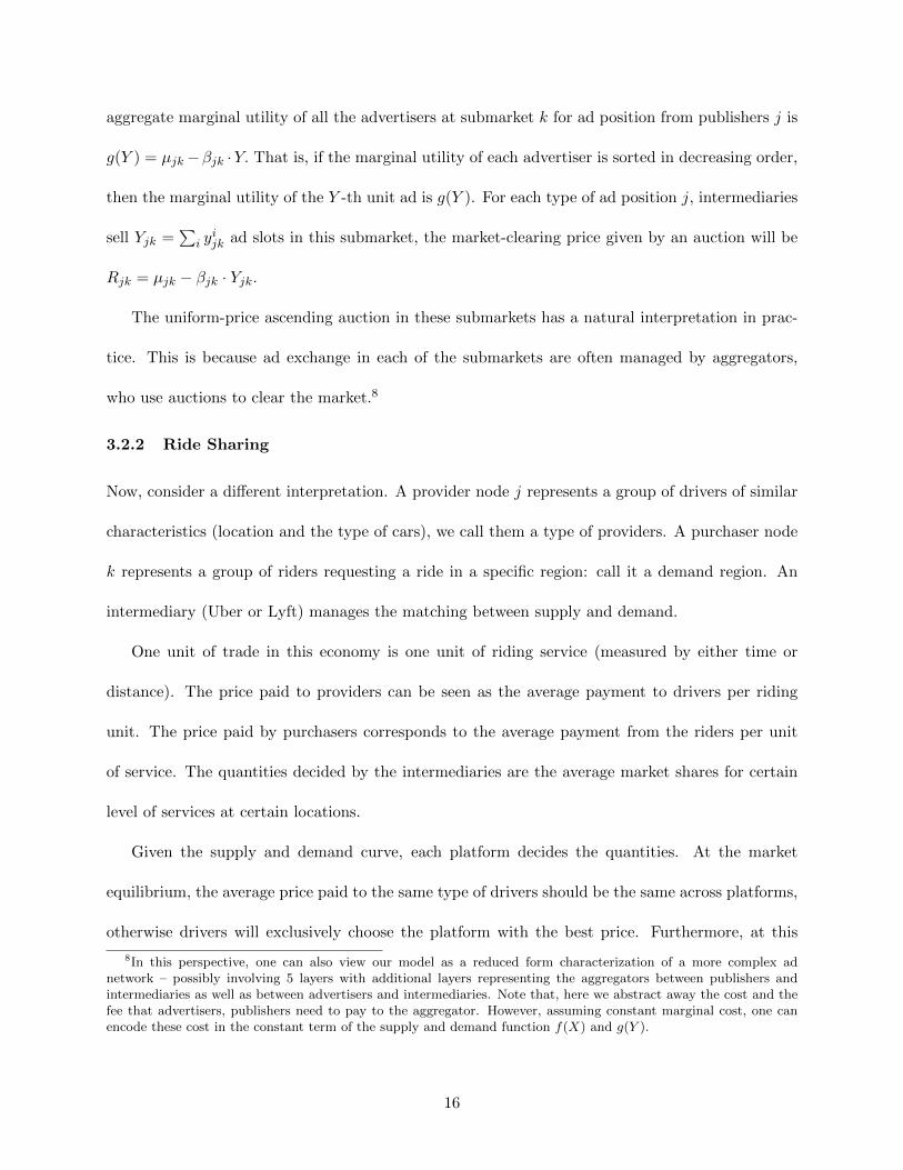
aggregate marginal utility of all the advertisers at submarket k for ad position from publishers j is

g(Y ) = µjk−βjk ·Y. That is, if the marginal utility of each advertiser is sorted in decreasing order,

then the marginal utility of the Y -th unit ad is g(Y ). For each type of ad position j, intermediaries

sell Yjk =∑

i yijk ad slots in this submarket, the market-clearing price given by an auction will be

Rjk = µjk − βjk · Yjk.

The uniform-price ascending auction in these submarkets has a natural interpretation in prac-

tice. This is because ad exchange in each of the submarkets are often managed by aggregators,

who use auctions to clear the market.8

3.2.2 Ride Sharing

Now, consider a different interpretation. A provider node j represents a group of drivers of similar

characteristics (location and the type of cars), we call them a type of providers. A purchaser node

k represents a group of riders requesting a ride in a specific region: call it a demand region. An

intermediary (Uber or Lyft) manages the matching between supply and demand.

One unit of trade in this economy is one unit of riding service (measured by either time or

distance). The price paid to providers can be seen as the average payment to drivers per riding

unit. The price paid by purchasers corresponds to the average payment from the riders per unit

of service. The quantities decided by the intermediaries are the average market shares for certain

level of services at certain locations.

Given the supply and demand curve, each platform decides the quantities. At the market

equilibrium, the average price paid to the same type of drivers should be the same across platforms,

otherwise drivers will exclusively choose the platform with the best price. Furthermore, at this

8In this perspective, one can also view our model as a reduced form characterization of a more complex adnetwork – possibly involving 5 layers with additional layers representing the aggregators between publishers andintermediaries as well as between advertisers and intermediaries. Note that, here we abstract away the cost and thefee that advertisers, publishers need to pay to the aggregator. However, assuming constant marginal cost, one canencode these cost in the constant term of the supply and demand function f(X) and g(Y ).

16

price amount of service offer by the drivers should be the same as the the total market share across

platforms. The same logic holds for the riders. The Cournot competition exactly captures this

aspect of competition. Namely, depending on the number of rides enabled, the market price will

be endogenously determined depending on the demand and supply curves of the providers and

purchasers. Specifically, we assume each provider in j has an increasing marginal cost for providing

service. It gives rise to the supply curve increasing in Pj , which we assume is:

Xj = max0, a · Pj − b.

Similarly, the demand curve at a demand region k for a specific type of provider j decreases in the

price Rjk, and is assumed to be:

Yjk = max0, b′ − a′ ·Rjk.

By changing notation a, b, a′, b′, we obtain equivalently Equations (1) and (2).

3.3 Summary of Characterizations and Definitions

In summary, we consider a networked market involving intermediaries and heterogeneous purchasers

and providers. Even though such markets tend to be highly dynamic market in reality, we study

their equilibrium in a “steady” state. This can be modeled as a single period game involving multiple

intermediaries each of which chooses yijk. Recall that these choices determine Xj , which affect the

inverse supply function; and Yjk which affect the inverse demand function on the purchaser sides.

They in turn determine the prices to be paid to the producers and the revenues from the purchasers.

So, each intermediary i’s payoff is the difference between the money paid by the purchasers and

17

the amount paid to the providers:

Πi(~y) =∑jk

Rjkyijk −

∑j

Pj∑k

yijk, (3)

where ~y correspond to the vector of quantities chosen by the intermediaries, i.e., ~y = ~y1, ~y2, . . . , ~yI,

where each ~yi is a matrix corresponding to yijk. The game described above is denoted as Γ(N , θ, µ, α, β).

Then, we have the following definition of an equilibrium for the game:

Definition 3.1. ~y is an equilibrium if no intermediary i can change his stratergy ~yi to ~yi′ to obtain

a better payoff given by (3).That is,

Πi( ~y1, . . . ,~yi′ , . . . , ~yI) > Πi( ~y1, . . . , ~yi, . . . ,

~yI).

The game can be characterized as a bi-partite graph involving purchasers and producers, with

the edges having Yjk as the weights. This bipartite graph is useful when studying social welfare.

The total social welfare is a measure of how efficient the allocation of providers to purchasers is.

We compute it by adding the total surplus of providers, purchasers and intermediaries:

Definition 3.2. Given a strategy profile ~y, social welfare is

SW (~y) =∑jk

Ujk(Yjk)−∑j

Cj(Xj) =∑jk

(µjkYjk −1

2βjkY

2jk)−

∑j

(θjXj +1

2αjX

2j ). (4)

4 Equilibrium Characterization

We illustrate the equilibrium with an example for two reasons. The first is to show how the variables

we defined earlier correspond to supply and demand functions. The second is to provide a figurative

perspective on social welfare.

18

Example 1. Consider the example with one provider, one purchaser, and one intermediary. The

intermediary’s decision variable is the amount, y, to buy from the provider and to deliver for the

purchaser. We assume that the marginal cost for the provider is 1 + y and the marginal gain for

the purchaser in the market is 2 − y. Then, the intermediary pays the provider P = 1 + y, and

charges the purchaser R = 2− y. So, the intermediary maximizes

maxy

R · y − P · y = (2− y)y − (1 + y)y

∣∣ y ≥ 0.

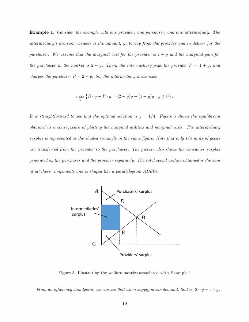
It is straightforward to see that the optimal solution is y = 1/4. Figure 3 shows the equilibrium

obtained as a consequence of plotting the marginal utilities and marginal costs. The intermediary

surplus is represented as the shaded rectangle in the same figure. Note that only 1/4 units of goods

are transferred from the provider to the purchaser. The picture also shows the consumer surplus

generated by the purchaser and the provider separately. The total social welfare obtained is the sum

of all these components and is shaped like a parallelogram ADECs.

A

B

C

Purchasers’ surplus

Providers’ surplus

Intermediaries’surplus

D

E

Figure 3: Illustrating the welfare metrics associated with Example 1

From an efficiency standpoint, we can see that when supply meets demand, that is, 2−y = 1+y,

19

we have the maximum welfare obtained when y = 1/2. This maximum welfare corresponds to the

area of the triangle ABC in the same figure. That corresponds to when the intermediary makes

zero profit. In this scenario involving only one provider and one purchaser, increasing the number

of intermediaries will always improve social welfare. However, that may not be the case when the

market structure and networks are different, as will be shown later.9

In general, equilibria are hard to characterize in games with complex network structure but

equilibrium always exists in our model. Furthermore, the equilibrium is unique and can be char-

acterized by a convex program. Hence, we can study the sensitivity of the network structure on

various metrics. This section characterizes the nature of the equilibrium.

Because xij =∑

k yijk, the payoff of intermediary i expressed in (3) can be written as

∑j,k(µjk − βjkYjk)yijk −

∑j(θj + αjXj)x

ij =

∑i,j,k

(µjk − θj)yijk −∑j,k

βjkYjkyijk −

∑j,k

αjXjyijk.

Observe that, for every i ∈ I, the utility function above can be seen as a concave function of ~y.

Furthermore, notice also a constant Z exists such that if yijk > Z then the payoff above is negative.

Therefore, the game we consider is a bounded, concave game. Because of Rosen (1965), such a

game has a pure equilibrium.

Given the specific payoff structure in our game, we can provide additional insights. For example,

the equilibrium is unique and can be characterized as follows:

Theorem 4.1. If αj > 0, and βjk > 0, ~y is an equilibrium if and only if it is the unique solution

9Note that, in this example, outside the Cournot competition framework, it is possible for the intermediary to offercontracts involving both price and quantity and the monopolist would obtain all the trade surplus. However, as inour applications, if each provider and purchaser represent a group of anynomous sellers and buyers, the intermediarywill not be able to extract all the surplus.

20

of the following convex program with the unknowns ~y, ~x, ~X, and ~Y :

min :∑

jαj2 (Xj)

2 +∑

ijαj2 (xij)

2 +∑

j,kβjk2 (Yjk)

2 +∑

i,j,kβjk2 (yijk)

2

s.t : αjXj + αjxij + βjkYjk + βjky

ijk ≥ µjk − θj . (5)

The formal proof is given in Appendix A.

Remark 4.2. To gain some further intuition of the game, consider a centralized agent who on

behalf of all the intermediaries facilitates trade between providers and purchasers to maximizes

welfare. The agent’s problem reduces to an optimization problem on the variables Yjk of the

bipartite network for the pairs (j, k) that are connected by at least one intermediary. The objective

of that optimization problem is to maximize the total utility of the purchasers minus the total cost

of the providers. Assume Y ∗jk is the welfare-maximizing solution.

In the equilibrium, each intermediary i individually decides on a set of yijk, where (j, k) are

connected via i. First, compared with the hypothetical centralized agent, the set of trade (j, k) that the

intermediary i can control is smaller. Second, multiple intermediaries can decide different amounts

of trade on a pair of (j, k). The total trade resulting in equilibrium between j, k is Yjk =∑

i yijk.

Third, the intermediaries are payoff maximizers. Our paper studies how far away the equilibrium

outcome Yjk is from the welfare-maximizing solution Y ∗jk.

Hence, from a welfare perspective, the tripartite graph reduces to a bipartite structure. We

exploit this feature in Section 6. However, to understand the equilibrium behavior, the structure

of the original tripartite graph is important because it captures the set of possible trades between

providers and purchasers that a particular intermediary can transact.

21

5 Insights from Networks: Increasing Competition and Merging Intermediaries

Having established the equilibrium, we can now identify insights about the effect of network struc-

tures on market efficiency. In particular, we provide two illustrative examples. The first shows

that increasing competition is not always beneficial for market efficiency. The second shows that

mergers have an ambiguous effect on efficiency. These examples highlight two insights into market

inefficiency caused by intermediaries, that are absent in standard Cournot models.

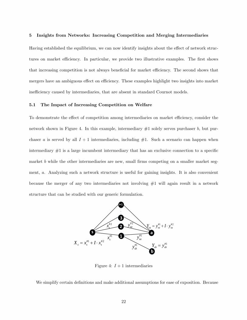
5.1 The Impact of Increasing Competition on Welfare

To demonstrate the effect of competition among intermediaries on market efficiency, consider the

network shown in Figure 4. In this example, intermediary #1 solely serves purchaser b, but pur-

chaser a is served by all I + 1 intermediaries, including #1. Such a scenario can happen when

intermediary #1 is a large incumbent intermediary that has an exclusive connection to a specific

market b while the other intermediaries are new, small firms competing on a smaller market seg-

ment, a. Analyzing such a network structure is useful for gaining insights. It is also convenient

because the merger of any two intermediaries not involving #1 will again result in a network

structure that can be studied with our generic formulation.

#1 #2s s sX x I x= + ⋅

3

1

b

#2say

#1say

#1sby

#2sx

#1sx

#1 #2sa sa saY y I y= + ⋅

#1sb sbY y=

.

.

.

2

I+1

as

Figure 4: I + 1 intermediaries

We simplify certain definitions and make additional assumptions for ease of exposition. Because

22

there is only one provider, we simply denote α = αs, µsa = µa, and µsb = µb. The additional

assumptions we make are as follows: θs = 0 for the providers; and β = βsa = βsb for the purchasers.

Because intermediaries 2, 3, . . . , I + 1 are symmetric, y#jsa = y#2sa and x#jsa = x#2

sa for any 1 < j ≤

I + 1.10 The equilibrium is therefore the optimal solution to the following program:

min : α(

(Xs)2 + I(x#2

s )2 + (x#1s )2

)+ β

((Ysa)

2 + I(y#2sa )2 + (y#1

sa )2)

+ β(

(Ysb)2 + (y#1

sb )2)

s.t : αXs + αx#2s + βYsa + βy#2

sa ≥ µa

αXs + αx#1s + βYsa + βy#1

sa ≥ µa

αXs + αx#1s + βYsb + βy#1

sb ≥ µb.

Notice that α and β capture the market sensitivity of the provider (seller) and the purchasers

(buyers), respectively. We next consider two extreme cases in order to gain intuition about this

network structure. The first has α = 1, β = 0, and the second has α = 0, β = 1. The main insight

continue to hold for a wider range of α, β (see Appendix B)

Case 1: α = 1, β = 0. This scenario corresponds to the case, where the marginal utility of the

purchasers is much less sensitive to the amount of good traded compared with the marginal cost of

the supply side. With this, we obtain the following result.

Corollary 5.1. α = 1, β = 0,

• µa < µb <54µa as I increases, the welfare will first increase and, then decrease.

• 54µa ≤ µb < 2µa, as I increases, the welfare will decrease.

• 2µa ≤ µb the welfare is independent of I.

10The argument to prove is as follows. Suppose that is not the case and one of those values is not equal atequilibrium. Then, because the constraints are identical for other intermediaries, the different solution should havebeen optimal for the every other intermediary also. We also know from Theorem 4.1 that the equilibrium is unique.

23

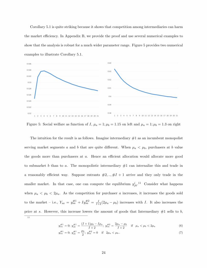
Corollary 5.1 is quite striking because it shows that competition among intermediaries can harm

the market efficiency. In Appendix B, we provide the proof and use several numerical examples to

show that the analysis is robust for a much wider parameter range. Figure 5 provides two numerical

examples to illustrate Corollary 5.1.

0.52

0.522

0.524

0.526

0.528

0.53

0.532

0.534

0.536

1 2 3 4 5 6 7 8 9 10 11 12 13 14 15 16 17 18 19 20 210.58

0.59

0.6

0.61

0.62

0.63

0.64

1 2 3 4 5 6 7 8 9 10 11 12 13 14 15 16 17 18 19 20 21

Figure 5: Social welfare as function of I, µa = 1;µb = 1.15 on left and µa = 1;µb = 1.3 on right

The intuition for the result is as follows. Imagine intermediary #1 as an incumbent monopolist

serving market segments a and b that are quite different. When µa < µb, purchasers at b value

the goods more than purchasers at a. Hence an efficient allocation would allocate more good

to submarket b than to a. The monopolistic intermediary #1 can internalize this and trade in

a reasonably efficient way. Suppose entrants #2, ..,#I + 1 arrive and they only trade in the

smaller market. In that case, one can compute the equilibrium yijk.11 Consider what happens

when µa < µb < 2µa. As the competition for purchaser a increases, it increases the goods sold

to the market – i.e., Ysa = y#1sa + Iy#2

sa = II+2(2µa − µb) increases with I. It also increases the

price at s. However, this increase lowers the amount of goods that Intermediary #1 sells to b,

11

y#1sa = 0; y#1

sb =(I + 1)µb − Iµa

I + 2; y#2

sa =2µa − µbI + 2

if µa < µb < 2µa (6)

y#1sa = 0; y#1

sb =µb2

; y#2sa = 0 if 2µa < µb.. (7)

24

Ysb = (µb − µa) + 2µa−µbI+2 . When 5

4µa ≤ µb < 2µa, delivering goods to b is preferred from social

standpoint. When I increases in that case, the competition in market a only distorts the trade

further away from the efficient allocation.

Next, consider the impact of competing intermediaries on the share of the surplus. When

µb > 2µa, intermediaries #2, . . . , I + 1 do not participate, and the equilibrium is independent of I.

So, we focus on the more interesting case µa ≤ µb ≤ 2µa, in which we obtain the following result.

Corollary 5.2. α = 1, β = 0 and µa ≤ µb ≤ 2µa,

• as I increases, provider s’s and purchaser a’ payoff increase; but b’s utility decreases.

• The payoff of all the intermediaries decreases as I increases.

See Appendix B.2 for the proof.

Case 2: α = 0, β = 1. The negative effect of competition on welfare described above is driven

partly by the fact that price at the providers is more sensitive to the amount of goods traded than

the price at the purchasers. As we see from the calculation above, because of this, when the number

of intermediaries increases, the competition pushes the selling down the price at the provider. We

will show next to that this effect disappears when the price at the providers is not sensitive to the

amount of goods traded.

Corollary 5.3. α = 0, β = 1, increasing the number of intermediaries will make the market more

competitive and improve social welfare. However, intermediary #1 remains as the monopoly for

purchaser b.

To see this, observe that the value of goods allocated to purchasers is a diminishing marginal

function. Thus, the most efficient way to allocate goods is when these marginals are 0, that is,

allocate µa and µb amount of goods to purchaser a and b, respectively. The convex program above

25

defines the equilibrium for this game as:

y#1sb =

µb2

; y#1sa = y#2

sa =µaI + 2

From this, we can calculate the amount of goods allocated to purchaser a to be I+1I+2µa; and to

purchaser b to be µb2 .

5.2 The Impact of Mergers on Welfare

Next, we demonstrate another ‘counter-intuitive’ effect on welfare caused by merging intermediaries.

For this, we consider the same network and the two scenarios shown in Figure 1. In scenario I, three

intermediaries A, B, and C compete to deliver goods between purchasers 3 and 4 and providers 1

and 2. In scenario II, A and B merge. Notice that in scenario I, A and B compete to deliver goods

from 1 to 4, but C is the only intermediary between 2 and 3. However, when A and B merge, the

merged firm AB becomes the monopoly between 1 and 4, but a competitor for C between 2 and 3.

Depending on how purchaser 3 values the goods from provider 2 relative to the valuations for

the other purchaser-provider pairs, the merging of A and B may or may not improve social welfare.

Interestingly, for a wide range of parameter values, merging A and B improves consumer welfare.

A more specific analysis is given in the following result.

Corollary 5.4. Consider the network in Figure 1 and the following set of parameters αj = 1,

furthermore, µ23 = V ;β23 = 1, µ13 = µ24 = 0;β13 = β24 = 0;µ14 = 1;β14 = 1; θj = 0.

If V > 1, then the revenue of AB after the merger is larger than the combined revenue of A

and B before the merger; furthermore, both the social welfare and the consumer surplus in scenario

II are also larger than in scenario I.

If 3/7 < V < 1, then the revenue of AB after the merger is less than the combined revenue of

A and B before the merger; furthermore, the social welfare in scenario II is also less than that in

26

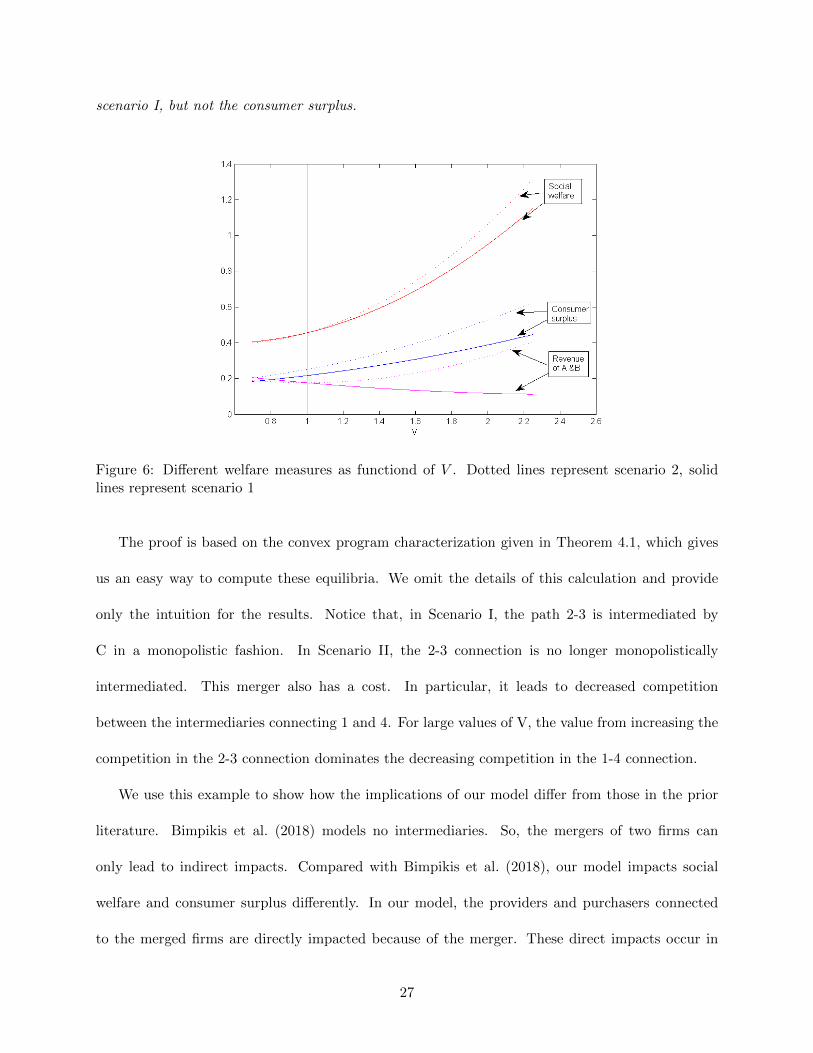
scenario I, but not the consumer surplus.

Figure 6: Different welfare measures as functiond of V . Dotted lines represent scenario 2, solidlines represent scenario 1

The proof is based on the convex program characterization given in Theorem 4.1, which gives

us an easy way to compute these equilibria. We omit the details of this calculation and provide

only the intuition for the results. Notice that, in Scenario I, the path 2-3 is intermediated by

C in a monopolistic fashion. In Scenario II, the 2-3 connection is no longer monopolistically

intermediated. This merger also has a cost. In particular, it leads to decreased competition

between the intermediaries connecting 1 and 4. For large values of V, the value from increasing the

competition in the 2-3 connection dominates the decreasing competition in the 1-4 connection.

We use this example to show how the implications of our model differ from those in the prior

literature. Bimpikis et al. (2018) models no intermediaries. So, the mergers of two firms can

only lead to indirect impacts. Compared with Bimpikis et al. (2018), our model impacts social

welfare and consumer surplus differently. In our model, the providers and purchasers connected

to the merged firms are directly impacted because of the merger. These direct impacts occur in

27

addition to the indirect ones. Therefore, unlike theirs, we can study the implications of mergers of

intermediaries. In conclusion, this section demonstrates that social welfare implications critically

depend on the network structure. Comparing two arbitrary networks is, in general, a difficult task,

and mergers can have both positive and negative welfare implications. While we have studied

interesting policy questions thus far, we are also interested in studying how close we can get to the

social optima. Specifically, we are interested in bounding the efficiency loss. Additionally, we are

interested in analyzing how the parameters of our model may affect the efficiency-loss bounds.

6 Bounding Inefficiency

This section builds further on the previous section to show how network structure influences effi-

ciency. Our intent is to act as a guide for market designers or policymakers to evaluate alternative

network structures from an efficiency standpoint. We specifically study how the network structures

lead the social welfare obtained in the decentralized context compared with the optimal one (with-

out any such constraint). For this purpose, we use the measure called price of anarchy which is the

ratio between the welfare of a Nash equilibrium and the optimal social welfare without incentive

constraints. This measure is studied in Dubey (1986) and is extensively used in computer science

starting with Koutsoupias and Papadimitriou (1999). If this ratio is close to 1, then it means that

the system is almost optimal.

28

6.1 Price of Anarchy: Lower Bound

Definition 6.1. Let E ⊂ J × K be the set of node pairs j ∈ J ; k ∈ K. Define OPT (E) as the

optimal social welfare obtainable through the links in E, that is,

OPT (E) := maxX,Y

∑j,k

µjkYjk −∑j

θjXj −∑jk∈E

βjkY 2jk

2−∑j∈J

αjX2j

2. (8)

s.t : X,Y ≥ 0

Yjk = 0 ∀jk /∈ E

Xj =∑k

Yjk.

If the set of connections (or links) in E constrain the trades to occur only between the connected

(or linked) agents, OPT (E) is the maximum level of welfare the system can achieve. In our

environment, a trade between j ∈ J and k ∈ K is possible only if they are connected to at least a

common intermediary. Let E1 ⊂ J ×K be the set of such pairs. Namely,

E1 := (j, k) ∈ J ×K| there exists i ∈ I where both ji and ik are connected.

Thus, at the equilibrium, the welfare is at most OPT (E1). Our first Price of Anarchy result

provides a lower bound on the welfare of the equilibrium compared with OPT (E1).

Theorem 6.2. The social welfare at the Nash equilibrium of the game Γ(N , θ, µ, α, β) (defined in

Definition 3.1) is at least 2/3 times the optimal social welfare, OPT (E1).

The proof of this theorem is provided in Appendix C. There, we establish the equilibrium to

be a series of inequalities. Using those inequalities, we determine the lower bound on the efficiency

of the system. This lower bound of 23 is called the price of anarchy (PoA). It measures the extent

to which selfish behavior affects efficiency. Note that this result differs from that of the Bertrand

29

competition model among intermediaries in Blume et al. (2009). In their model, all equilibria are

efficient, and so merging of intermediaries would not change the price of anarchy.

6.2 Price of Anarchy: Refined Lower Bound

While it is a general result, Theorem 6.2 does not provide information about the role of the un-

derlying network structure on welfare. For example, in Figure 1, it may be interesting to obtain

a more detailed efficiency comparison of the two networks. To obtain more general bounds that

reveal the structure of networks, the following notions of network connectivity are important.

Definition 6.3. Given a network G whose nodes are partitioned into three disjoint classes J, I,K.

We define the edges of G to be those that connect nodes between J, I, and between I,K, while J,K

are disconnected. We define the ω-th layer of G, denoted as Eω(G) or Eω for short, to be the set

of node pairs jk : j ∈ J ; k ∈ K that are connected by at least ω nodes i ∈ I (that is both ji and ik

are edges in G).

For example, for each of the networks in Figure 1, the first layer of G, ω = 1, contains the pairs

13, 14, 23, 24. The 2nd layer of the network, ω = 2, in scenario I (on the left-hand side) is the

pair 14, and in Scenario II is the pair 23. Given this definition, our next result refines the price of

anarchy for these layers of the network.

Theorem 6.4. Given a network G over the set of providers, purchasers and intermediaries the

social welfare at the Nash equilibrium is at least (1− 12ω+1)OPT (Eω).

The proof of Theorem 6.4 is given in Appendix D. Relative to Theorem 6.2, Theorem 6.4 is

informative about the level of efficiency in a more refined way. In particular, Theorem 6.4 suggests

more details on the influence of the underlying network structure on the level of efficiency. To

illustrate, continue with the example network in Figure 1. With ω = 2, Theorem 6.4 implies

that the welfare at equilibrium in the network on the left-hand side is at least 4/5 times the total

30

trade surplus of the submarket between 1 and 4, and for the network on the right-hand side, its

equilibrium welfare is at least 4/5 times the total trade surplus of the submarket between 2 and 3.

This means that merging A and B is beneficial under a Nash model if the submarket between 2

and 3 has high trade value.

This theorem can be insightful for a network designer when analyzing policies having substantial

changes in the network structure. The designer should consider policy impacts on different layers

of the network. In particular, there is a trade-off in the bound (1 − 12ω+1)OPT (Eω): OPT (Eω)

is decreasing, while (1 − 12ω+1) is increasing in ω. Hence, the layer of the network that closest

captures the efficiency of the equilibrium is the one that has both high connectivity ω, and high

trade maximum value, OPT (Eω). Significant changes in this network layer will likely have a large

impact on the efficiency of the market. In the remainder of this section, we further discuss the

implications of this result. Here, we will consider the price of anarchy as the proxy for the efficiency

of the market and study the impact of the “intermediary capacity” on this measure of efficiency.

6.3 Impact of Intermediary Capacity on Price of Anarchy

We start by defining a parameter, which we call the intermediary capacity of the network.

Definition 6.5. For a node pair j ∈ J ; k ∈ K in the network G, which are connected by at least

one middleman, let wjk ≥ 1 be the number of middlemen that connect j and k. Then, wG, called

the intermediary capacity of G, is defined as the minimum value among all such wjk.

The intermediary capacity of the network, wG, is a measure of the competitiveness of the

network market. For any provider and purchaser that can potentially trade through the network,

they can trade by at least wG intermediaries. Further, as a corollary of Theorem 6.4, we obtain

the following result:

Corollary 6.6. The price of anarchy is at least 1− 12wG+1 .

31

Because wG ≥ 1 for any network G Corollary 6.6 is a generalization of Theorem 6.2, note that

the intermediary capacity of the network intuitively captures the degree of competition among the

intermediaries. As the intermediary capacity of the network increases – i.e., as the economy becomes

more competitive – the system approaches full efficiency. Note that while mergers can lower the

intermediary capacity, it is not always the case, as illustrated by the example in Figure 1. So,

Corollary 6.6 does not contradict our earlier result that mergers can have ambiguous implications

for welfare.

7 Extension for Subsitute Goods

Previously, we assumed that the utility of k as additive across j i.e.,∑

j Ujk(Yjk). In this section,

we consider the case where the goods are a substitute. We show that a similar characterization

of equilibrium based on a convex program applies but it is even simpler. Recall that yijk is the

amount of goods that intermediaries i provided by j to k; the total amount of good that i sells to

k is Y ik =

∑j y

ijk; the total amount of good that i buys from j is xij =

∑k y

ijk; and Yk =

∑j Yjk

is the total amount of goods that a purchaser k obtains. We assume the utility of a purchaser k is

Uk(Yk) = µkYk − 12βkY

2k . Thus the marginal price at the purchaser k is

∂Uk(Yk)

∂Yk= µk − βkYk.

We further assume a unit cost of cjk ≥ 0 that the intermediary needs to pay i for delivering

goods from j to k.12 Then, intermediary i’s payoff function is

Φ(y) =∑k

(µk − βkYk)Y ik −

∑jk

cjkyijk −

∑j

(θj + αjXj)xij

12The analysis extends for the case that each intermediary i has a different cost cijk.

32

Given an index j∗ and k∗, taking derivative according to yij∗k∗ we obtain:

∑k

(µk − βkYk)∂Y i

k

∂yij∗k∗+∑k

∂(µk − βkYk)∂yij∗k∗

Y ik − cj∗k∗ −

∑j

(θj + αjXj)∂xij∂yij∗k∗

−∑j

∂(θj + αjXj)

∂yij∗k∗xij

Notice that if k 6= k∗, then∂Y ik∂yij∗k∗

= 0, and if j 6= j∗, then∂xij

∂yij∗k∗

= 0. Thus,

∂Φ(y)

∂yij∗k∗= (µk∗ − βk∗Yk∗)− βk∗Y i

k∗ − cj∗k∗ − (θj∗ + αj∗Xj∗)− αj∗xij∗ .

Observe that Φ(.) is a concave function, thus, we have the following first order condition for an

equilibrium for all provider j∗, purchaser k∗ and intermediary i, who are connected in the network.

αj∗Xj∗ + αj∗xij∗ + βk∗Yk∗ + βk∗Y

ik∗ ≥ µk∗ − θj∗ − cj∗k∗

if strict inequality holds then yij∗k∗ = 0.

Given this equilibrium condition, using a similar argument as in Theorem 4.1, we obtain the

following characterization of equilibria. The proof of this result is provided in Appendix E.

Theorem 7.1. The equilibrium is unique and is the solution of the following convex program

min∑j

αj(Xj)2 +

∑j,i

αj(xij)

2 +∑k

βk(Yk)2 +

∑i,k

βk(Yik )2 (9)

sjt : αjXj + αjxij + βkYk + βkY

ik ≥ µk − θj − cjk ∀j, k, i where i connects j and k. (10)

This theorem suggests that even when the purchasers consider goods from different providers

substitutes, the equilibrium is unique and characterized by a convex program. Hence, the results

in the previous section extend to this case as well.

33

8 Conclusions And Future Work

Sharing economies facilitated by multisided platforms are becoming increasingly popular in many

contexts (Uber, Airbnb being some of the well-known ones). Therefore, understanding the welfare

implications of these platforms is important to guide policy proposals for improving social welfare.

For example, as the sharing economy matures, mergers, and acquisitions among platforms are likely

to occur. Yet, there is little guidance from the prior literature to analyze the welfare implications

of such mergers. This is because the majority of the current literature focuses on monopoly pricing

problems. Our paper fills this void by developing a tractable model that provides insights into the

role of network structure in affecting welfare.

The contributions of our paper are twofold. First, we show that in the presence of intermediaries

and networks, mergers and competition have an ambiguous effect on welfare. These effects are

absent in models of prior literature that are without networks/intermediaries. Second, we introduce

a measure of intermediary capacity that gives an upper bound on the loss of efficiency. As the

intermediary capacity gets bigger, the loss of efficiency approaches zero. These nontrivial and robust

structural results potentially have policy implications on evaluating mergers of intermediaries.

Even though we presented the analysis in a stylized context, the underlying structure is relevant

more broadly. For example, the analysis is also relevant to a physical retail chain context. Visualize

the retailers as the platform companies. On one side of the network are manufacturers (e.g., Reebok,

Under Armour). On the other side of the network are geographic locations where the retailers

compete against one another. The edges between the first side and the platform now correspond to

whether the retailer carries the products from the manufacturers. The edges between the platform

and the second side correspond to whether the retailer has a presence in the geographic location.

In such a context, our insights become relevant when studying the impact of retail chain mergers.

Additionally, the insights continue to be valid in some variations of our model. For example, in

34

the ad-auction context, a provider can correspond to supply aggregator firms such as ValueClick,

AdBrite, Burst Media, etc. So, the network may involve an additional layer, say 4-partite graph

with advertisers connecting to the ad aggregators connecting to the intermediaries. If we assume

that the value perceived at those ad-aggregator nodes does not change because of mergers of

intermediaries, then the current analysis is not affected by extending the graph. This implies that

analyzing the three-layer network structure is informative enough for the efficiency of the market.

However, if the valuations at the provider nodes change because of changes to the market

structure, then the multi-partite graph would be needed, which we leave for future work. In essence,

we have considered a parsimonious structure for analysis which is robust to some generalizations.

In conclusion, we have provided a tractable model of competition among intermediaries. Our

key results show that the traditional antitrust analysis does not apply to a platform context because

of the nature of the underlying network. As mentioned earlier, it would be of interest to study more

deeply in the future the welfare implications when characterizing a multi-partite graph involving

aggregators on the publisher- and/or the provider-side; or when purchasers can easily substitute

among the offerings. Furthermore, for future work, it would be also of interest to model more

general utility functions, uncertainty, asymmetric information, and network formation questions.

Moreover, we used the Cournot model as the basis for the information structure in our model and

this allowed us to not focus on price+quantity contracts. Another possible extension is to study a

detailed model involving such contracts.

APPENDIX

A Proof of Theorem 4.1

Proof. We first illustrate the main idea of the proof with an example of the network in Figure 7. The

example will also subsequently be used to demonstrate some seemingly counterintuitive results when

35

#1 #2s s sX x x= +

2

1 a

b

#2say

#1say

#1sby

#2sx

#1sx

s

#1 #2sa sa saY y y= +

#1sb sbY y=

#2 #2s sax y=

1 #1 #1s sa sbx y y= +

Figure 7: Illustrating example for equilibrium

we later study the sensitivity of the results. As for the example, assume a networked structured as

in Figure 7, with two intermediaries (#1 and #2), two purchasers (a and b), and a provider (s).

Readers not interested in the characterization of the proof may skip to the end of the section.

We will use the optimality conditions of individual players’ payoffs to characterize the equilib-

rium. We already know that, at equilibrium, the inventory constraints imply x#1s = y#1

sa + y#1sb

and x#2s = y#2

sa . Further, Intermediary #2 connects seller s and purchaser a and so x#2s = y#2

sa .

Therefore, we can write the payoff of Intermediary #2 as functions of y:

Π2(y) = (µsa − βsaYsa)y#2sa − (θs + αsXs)x

#2s

= (µsa − βsaYsa)y#2sa − (θs + αsXs)y

#2sa

= (µsa − θs)y#2sa − βsaYsay#2

sa − αsXsy#2sa .

Notice that Ysa = y#2sa + y#1

sa and Xs = x#2s + x#1

s = y#2sa + y#1

sa + y#1sb , which are functions of y#2

sa .

Thus, the derivative of Π2(y) according to y#2sa is

∂Π2(y)

∂y#2sa

= (µsa − θs)− βsaYsa − βsay#2sa

∂Ysa

∂y#2sa

− αsXs − αsy#2sa

∂Xs

∂y#2sa

= (µsa − θs)− βsaYsa − βsay#2sa − αsXs − αsy#2

sa

36

Because Π2(y) is concave, we obtain the following necessary condition for Π2(y) to be optimal:

if y#2sa > 0 then

∂Π2(y)

∂y#2sa

= 0 and if∂Π2(y)

∂y#2sa

< 0, then y#2sa = 0. (11)

Similarly, for intermediary #1, with x#1s = y#1

sa + y#1sb , his payoff is:

Π1(y) = (µsa − βsaYsa)y#1sa + (µsb − βsbYsb)y#1

sb − (θs + αsXs)x#1s

= (µsa − θs)y#1sa + (µsb − θs)y#1

sb − βsaYsay#1sa − βsbYsby

#1sb − αsXs(y

#1sa + y#1

sb ).

Taking derivative of Π1 according to y#1sa and y#1

sb we have

∂Π1(y)

∂y#1sa

= (µsa − θs)− βsaYsa − βsay#1sa

∂Ysa

∂y#1sa

− αsXs − αs(y#1sa + y#1

sb )∂Xs

∂y#1sa

= (µsa − θs)− βsaYsa − βsay#1sa − αsXs − αs(y#1

sa + y#1sb )

= (µsa − θs)− βsaYsa − βsay#1sa − αsXs − αsx#1

s .

∂Π1(y)

∂y#1sb

= (µsb − θs)− βsbYsb − βsby#1sb

∂Ysb

∂y#1sb

− αsXs − αs(y#1sa + y#1

sb )∂Xs

∂y#1sb

= (µsb − θs)− βsbYsb − βsby#1sb − αsXs − αs(y#1

sa + y#1sb )

= (µsb − θs)− βsbYsb − βsby#1sb − αsXs − αsx#1

s .

The first order conditions for Π1(y) to be optimal are

if y#1sa > 0 then

∂Π1(y)

∂y#1sa

= 0 and if∂Π1(y)

∂y#1sa

< 0, then y#1sa = 0 (12)

if y#1sb > 0 then

∂Π1(y)

∂y#1sb

= 0 and if∂Π1(y)

∂y#1sb

< 0, then y#1sb = 0. (13)

37

Let Ω = αs2

((Xs)

2 + (x#2s )2 + (x#1

s )2)

+ βsa2

((Ysa)

2 + (y#2sa )2 + (y#1

sa )2)

+ βsb2

((Ysb)

2 + (y#1sb )2

).

Next, consider the optimal solution of the following quadratic program:

min : Ω (14)

s.t : αsXs + αsx#2s + βsaYsa + βsay

#2sa ≥ µsa − θs. (15)

αsXs + αsx#1s + βsaYsa + βsay

#1sa ≥ µsa − θs. (16)

αsXs + αsx#1s + βsbYsb + βsby

#1sb ≥ µsb − θs. (17)

Let z#2sa , z

#1sa , z

#1sb be the dual variables of the constraints (15), (16), and (17), respectively. The

Lagrangian relaxation of this convex program is

Ω− z#2sa (αsXs + αsx

#2s + βsaYsa + βsay

#2sa − (µsa − θs))−

z#1sa (αsXs + αsx

#1s + βsaYsa + βsay

#1sa − (µsa − θs))−

z#1sb (αsXs + αsx

#1s + βsbYsb + βsby

#1sb − (µsb − θs)).

(18)

The first order conditions of the Lagrangian relaxation according to Xs give Xs = z#2sa + z#1

sa + z#1sb ;

according to x#2s give x#2

s = z#2sa ; according to x#1

s give x#1s = z#1

sa + z#1sb ; according to Ysa give

Ysa = z#2sa + z#1

sa ; according to Ysb give Ysb = z#1sb ; and according to y#2

sa give y#2sa = z#2

sa ; y#1sa gives

y#1sa = z#1

sa ; and y#1sb give y#1

sb = z#1sb .

Replacing z with y, we obtain a set of conditions that are exactly the equations of the game

captured in Figure 7. We need to show that the first order conditions of the payoff for intermediaries,

(11), (12), and (13) are also satisfied. Consider the first constraint (15). Notice that the KKT

conditions of the optimal solution of the convex program (14)-(16) imply that if the dual variable

z#2sa > 0, then the constraint binds, that is αsXs+αsx

#2s +βsaYsa+βsay

#2sa = µsa−θs. Furthermore,

if the constraint does not bind, i.e, αsXs + αsx#2s + βsaYsa + βsay

#2sa > µsa − θs, then z#2

sa = 0.

38

Notice that because z#2sa = y#2

sa , this condition is exactly the first order condition of for the payoff

of intermediary #1 in (11). Similarly, we can also have the equivalence between the equilibrium

condition of intermediary #2, (12) and (13), and the constraints (16) and (17). The example above

illustrates the equivalence between the equilibrium condition and the optimality of the quadratic

program (14) to (17). The same idea can be generalized to more general networks. In what follows,

we provide the formal proof.

The payoff for intermediary i is

Πi(y) =∑i,j,k

(µjk − θj)yijk −∑jk

βjkYjkyijk −

∑j,k

αjXjyijk

=∑i,j,k

(µjk − θj)yijk −∑jk

βjkYjkyijk −

∑j

αjXj

∑k

yijk.

The derivative of Πi(y) with respect to yijk is

∂Πi(y)

∂yijk= (µjk − θj)− βj,kYjk − βjkyijk − αjXj − αj

∑l∈K

yijl

= (µjk − θj)− βj,kYjk − βjkyijk − αjXj − αjxij

The above equation holds because xij =∑

l∈K yijl. Hence, the first order condition for y to be a

Nash equilibrium is the following:

(µjk − θj)− (βjkYjk + αjXj + αjxij + βjky

ijk) ≤ 0; and equality occurs if yijk > 0. (19)

We will show that (19) has a special property that allows us to characterize its unique solution

by a quadratic convex program. First, consider the unique solution of (5). By the complementarity

slackness condition, x, y,X, Y is the solution if for every i, j, k such that ij and ik are connected in

39

G, there exists a dual variable zijk satisfying

αj2 2Xj =

∑ik αjz

ijk (20)

αj2 2xij =

∑k αjz

ijk (21)

βjk2 2Yjk =

∑i βjkz

ijk (22)

βjk2 2yijk = (βjk)z

ijk. (23)

Furthermore,

if αjXj + αjxij + βjkYjk + βjky

ijk > µjk − θj , then zijk = 0. (24)

Observe that (23) implies that zijk = yijk. Therefore, from (20) , (21), and (22)

Xj =∑ik

yijk;xij =

∑k

yijk and Yjk =∑i

yijk.

Given this, (24) is equivalent to the first order condition in (19).

To see the reverse, given a ~z satisfying (19), we introduce zijk := yijk; Xj =∑

ik zijk;x

ij =∑

k zijk and Yjk =

∑i zijk. It is straightforward to see that z, x, y,X, Y satisfy (20-24). Therefore,

z, x, y,X, Y are actually the unique solution of the program (5).

B Proof of Corollary 5.1, 5.2 and Numerical examples

B.1 Proof of Corollary 5.1

First, if µb ≥ 2µa, then according to the equilibrium characterization, y#2sa = 0 and intermediary

1 will be the only active players. Thus the welfare of the system is independent of the number of

intermediaries I + 1.

It remains to consider the case µa < µb < 2µa. According to the equilibrium characterization,

40

the amount of goods delivered to a and b are

Ysa = y#1sa + Iy#2

sa =I

I + 2(2µa − µb) = 1− 2

(2µa − µb)I + 2

Ysb =(I + 1)µb − Iµa

I + 2= (µb − µa) +

2µa − µbI + 2

.

The total number of goods delivered is

Xs = Ysa + Ysb =Iµa + µbI + 2

= µa −2µa − µbI + 2

Denote t := 2µa−µbI+2 , the welfare is

µaYsa + µbYsb −1

2(Xs)

2 = µa(1− 2t) + µb(µb − µa + t)− 1

2(µa − t)2

= µa + µb(µb − µa)−1

2µ2a + (µb − µa)t−

1

2t2 =: f(t).

When I increases from 1 to ∞, t = 2µa−µbI+2 decreases from t1 := 2µa−µb

3 to t∞ := 0.

Notice that f(t) is a quadratic function and f ′(µb − µa) = 0. Thus, if t1 ≤ µb − µa, then f(t)

decreases if I increases; if t1 > µb − µa, then as I increases f(t) will first increase, then decrease.

Now, t1 = µb − µa implies µb = 5/4µa, which implies our result.

We consider two numerical examples where both α, β are positive.

Example 1: α = 1; β = 1; µa = 3;µb = 9 See Figure 8

Without intermediaries #2, 3, . . . , I+1, intermediary #1 will sell exclusively to purchaser b. y#1sa =

0; y#1sb = 2.25 and the welfare is 15.1875. With intermediary #2, the equilibrium is y#2

sa = 0.2; y#1sa =

0; y#1sb = 2.2 and the welfare is 15.08. As I increases, the social welfare decreases.

41

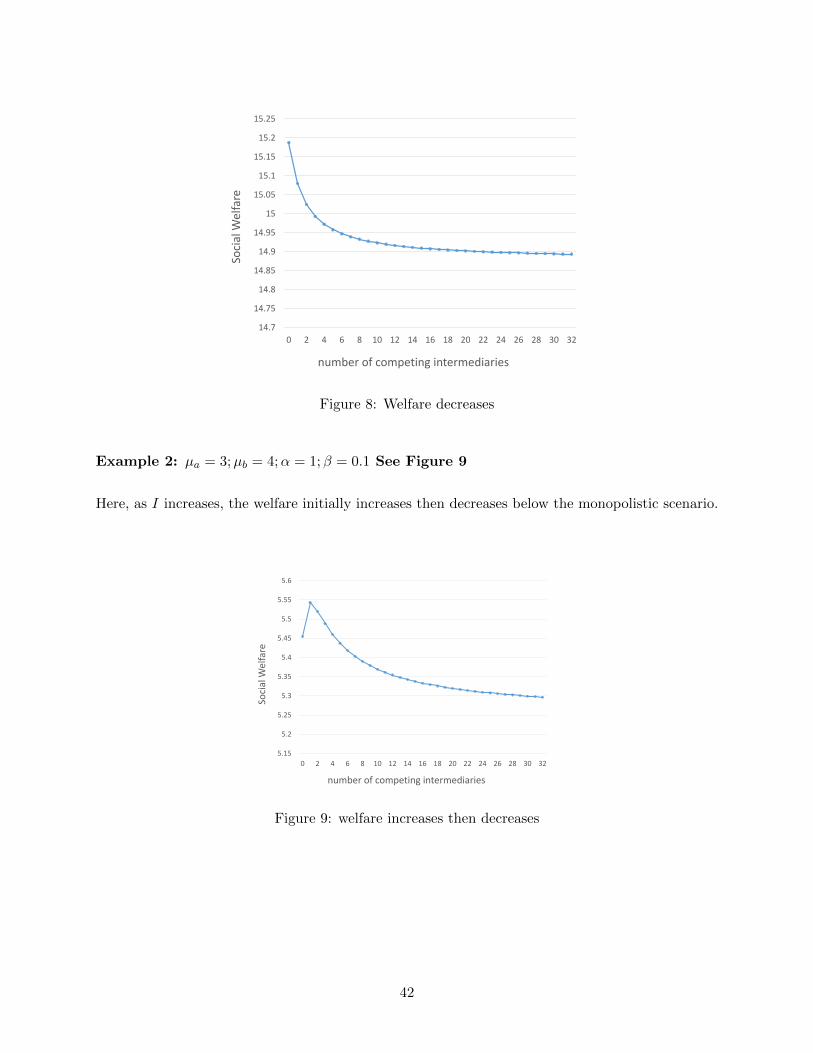
14.7

14.75

14.8

14.85

14.9

14.95

15

15.05

15.1

15.15

15.2

15.25

0 2 4 6 8 10 12 14 16 18 20 22 24 26 28 30 32

Soci

al W

elfa

re

number of competing intermediaries

Figure 8: Welfare decreases

Example 2: µa = 3;µb = 4;α = 1;β = 0.1 See Figure 9

Here, as I increases, the welfare initially increases then decreases below the monopolistic scenario.

5.15

5.2

5.25

5.3

5.35

5.4

5.45

5.5

5.55

5.6

0 2 4 6 8 10 12 14 16 18 20 22 24 26 28 30 32

Soci

al W

elfa

re

number of competing intermediaries

Figure 9: welfare increases then decreases

42

B.2 Proof of Corollary 5.2

Proof. According to the equilibrium computation (6) and (7), as I increases, the total amount of

goods s provides and the amount of goods a receives both increase. This shows that s and b’s payoff

increases. The amount of goods delivered to b, on the other hand decreases. As argued above, this

is a natural consequence of increasing competition for trade between s and a.

The formula for the payoff of intermediary 1 is µay#1sa +µby

#1sb −(y#1

sa +y#1sb )(Ysa+Ysb). Replacing

the solution of (6), we obtain that the payoff of intermediary 1 is

(µb − µa +2µa − µbI + 2

)2.

Thus, the payoff of intermediary 1 decreases as I increases. The payoff of each intermediary

2, 3, .., I + 1 is µay#2sa − y#2

sa (Ysa + Ysb) = (2µa−µbI+2 )2, which also decreases as I increases.

C Proof of Theorem 6.2

Proof. Let yijk be the Nash equilibrium. The social welfare with yijk as the decision is

SWNash =∑jk

(µjk∑i

yijk −βjk2Y 2jk)−

∑j

(θjXj +αj2X2j ).

Replacing Xj =∑

i,k yijk and Yjk =

∑i yijk, we have

SWNash =∑i,j,k

(µik − θj)ziik −∑jk

βjk2Y 2jk −

∑j

αj2X2j . (25)

Let cijk be the solution generating the optimal welfare, Aj =∑

i,k cijk, Bjk =

∑i cijk and

43

cij =∑

k cijk. The optimal social welfare is

SWOpt =∑i,j,k

(µjk − θj

)cijk −

∑jk

βjk2B2jk −

∑j

αj2A2j . (26)

Comparing SWNash and SWOpt, we observe that because of (19), we have

cijk((µjk − θj)− (αjXj + αjx

ij + βjkYjk + βjky

ijk))≤ 0.

Summing over all i, j, k we have

∑i,j,k

(µjk − θj)cijk −∑j

αjAjXj −∑ij

αjxijcij −

∑jk

βjkBjkYjk −∑i,j,k

βjkcijky

ijk ≤ 0. (27)

We use the following inequalities13

BjkYjk ≤1

3B2jk +

3

4Y 2jk;AjXj ≤

1

3A2j +

3

4X2j and

cijxij ≤

1

6(cij)

2 +3

2(xij)

2; cijkyijk ≤

1

6(cijk)

2 +3

2(yijk)

2

to apply to (27) to obtain the following inequality:

∑i,j,k(µjk − θj)cijk −

∑jαj3 A

2j −

∑ijαj6 (cij)

2 −∑

jkβjk3 B

2jk −

∑i,j,k

βjk6 (cijk)

2

≤ 32

(∑jαj2 X

2j +

∑ij αj(x

ij)

2 +∑

jkβjk2 Y

2jk +

∑i,j,k βjk(y

ijk)

2). (28)

To prove the theorem, we will show that the Left hand side of (28) is at least SWOpt and the

13These inequalities come from the fact that (γx− 12γy)2 ≥ 0 implies xy ≤ γ2x2 + 1

4γ2y2.

44

Right hand side of (28) is 32SWNash. Focusing on the Left hand side of (28), first observe that

∑ij

αj6

(cij)2 ≤

∑j

αj6

(∑i

(cij))2 =

∑j

αj6A2j , , and

∑i,j,k

βjk6

(cijk)2 ≤

∑jk

βjk6

(∑i

cijk)2 =

∑jk

βjk6B2jk.

Thus,

the left hand side of (28) ≥︸︷︷︸from (26)

∑i,j,k

(µjk − θj)cijk −∑j

αj2A2j −

∑jk

βjk2B2jk = SWOpt. (29)

Next, we will show that the right hand side of (28) is equal to SWNash. To see this, observe

that from the Nash equilibrium condition (19), we have

∑i,j,k

yijk ·((µjk − θj)− (αjXj + αjx

ij + βjkYjk + βjky

ijk))

= 0.

This is equivalent to

∑i,j,k

(µjk − θj)yijk =∑j

αjX2j +

∑ij

αj(xij)

2 +∑jk

βjkY2jk +

∑i,j,k

βjk(yijk)

2 (30)

Replacing∑

i,j,k(µjk − θj)yijk as in (30) to the formulation of the social welfare at Nash (25),

SWNash =∑

jαj2 X

2j +

∑ij αj(x

ij)

2 +∑

jkβjk2 Y

2jk +

∑i,j,k βjk(y

ijk)

2.

45

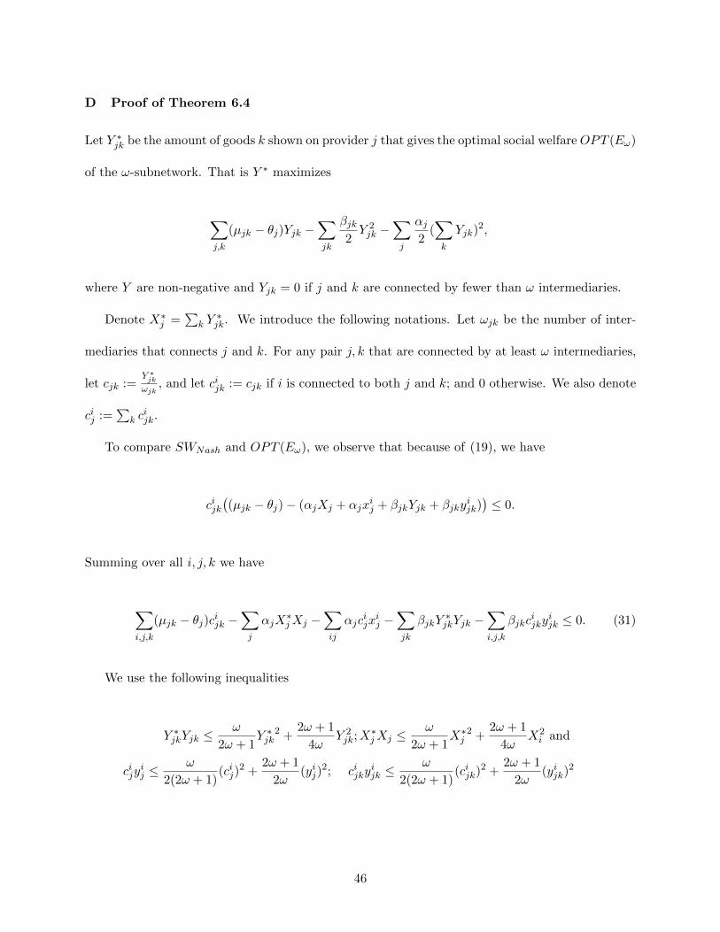
D Proof of Theorem 6.4

Let Y ∗jk be the amount of goods k shown on provider j that gives the optimal social welfareOPT (Eω)

of the ω-subnetwork. That is Y ∗ maximizes

∑j,k

(µjk − θj)Yjk −∑jk

βjk2Y 2jk −

∑j

αj2

(∑k

Yjk)2,

where Y are non-negative and Yjk = 0 if j and k are connected by fewer than ω intermediaries.

Denote X∗j =∑

k Y∗jk. We introduce the following notations. Let ωjk be the number of inter-

mediaries that connects j and k. For any pair j, k that are connected by at least ω intermediaries,

let cjk :=Y ∗jkωjk

, and let cijk := cjk if i is connected to both j and k; and 0 otherwise. We also denote

cij :=∑

k cijk.

To compare SWNash and OPT (Eω), we observe that because of (19), we have

cijk((µjk − θj)− (αjXj + αjx

ij + βjkYjk + βjky

ijk))≤ 0.

Summing over all i, j, k we have

∑i,j,k

(µjk − θj)cijk −∑j

αjX∗jXj −

∑ij

αjcijxij −

∑jk

βjkY∗jkYjk −

∑i,j,k

βjkcijky

ijk ≤ 0. (31)

We use the following inequalities

Y ∗jkYjk ≤ω

2ω + 1Y ∗jk

2 +2ω + 1

4ωY 2jk;X

∗jXj ≤

ω

2ω + 1X∗j

2 +2ω + 1

4ωX2i and

cijyij ≤

ω

2(2ω + 1)(cij)

2 +2ω + 1

2ω(yij)

2; cijkyijk ≤

ω

2(2ω + 1)(cijk)

2 +2ω + 1

2ω(yijk)

2

46

to apply to (31) and obtain the following inequality.

∑i,j,k

(µjk − θj)cijk −∑j

ω

2ω + 1αjX

∗j2 −

∑ij

ω

2(2ω + 1)αjc

ij2 −

∑jk

ω

2ω + 1βjkY

∗jk

2

−∑i,j,k

ω

2(2ω + 1)βjk(c

ijk)

2 ≤ 2ω + 1

2ω

(∑j

αj2X2j +

∑ij

αj(xij)

2 +∑jk

βjk2Y 2jk +

∑i,j,k

βjk(yijk)

2

)(32)

Similar to the proof of Theorem 6.2, the right hand side of (32) is 2ω+12ω SWNash. In order to

bound the left hand side of (32), we show the following.

ω∑i,j

(cij)2 ≤

∑j

(X∗j )2. (33)

ω∑i,j,k

(cijk)2 ≤

∑jk

(Y ∗jk)2. (34)

Assuming that (33) and (34) are true then the right hand side of (32) is at least

∑i,j,k

(µjk − θj)cijk −∑j

ω

2ω + 1αjX

∗j2 −

∑j

1

2(2ω + 1)αjX

∗j2 −

∑jk

ω

2ω + 1βjkY

∗jk

2

−∑jk

1

2(2ω + 1)βjkY

∗jk

2 =∑i,j,k

(µjk − θj)cijk −∑jk

1

2βjkY

∗jk

2 −∑j

1

2αjX

∗j2 = OPT (Eω). (35)

Hence, we conclude that OPT (Eω) ≤ 2ω+12ω SWNash, which is what we need to prove.

Thus, it remains to show that (33) and (34) are true. To see (34), observe that j, k are connected

by ωjk ≥ ω intermediaries, and by definition cijk =Y ∗jkωjk

. Thus,

Y ∗jk2 = ωjk ·

∑i,k

(cijk)2 ≥ ω ·

∑i,k

(cijk)2.

To see (33), observe that

(X∗j )2 = (∑k

Y ∗jk)2 = (

∑k

ωjkY ∗jkωik

)2 = (∑k

ωjkcjk)2 =

∑k

ω2jkc

2jk + 2

∑k<l

ωjkωjlcjkcjl. (36)

47

On the other hand, ∑i

(cij)2 =

∑i

(∑k

cijk)2. (37)

Notice that cijk = cjk if i is connected to both j and k and 0 otherwise. Thus, to bound∑

i(cij)

2,

we can bound the number of terms c2jk and cjkcjl that appear in (37). There are ωjk intermediaries

that connect to both j and k, thus c2jk appears exactly ωjk in (37). For k < l; the number of terms

cjkcjl that appear in (37) is twice the number of intermediaries who is connected to all three nodes

j, k and l. Hence the number of terms cjkcjl appearing in (37) is at most 2 minωjk, ωjl. So,

∑i

(cij)2 =

∑i

(∑k

cijk)2 ≤

∑k

ωjkc2jk + 2

∑k<l

minωjk, ωjlcjkcjl.

Comparing this and (36), we have ∑i

(cij)2 ≤ ω(X∗j )2,

which implies (33). With this we finish the proof.

E Proof of 7.1

Consider the convex program

min∑j

αj(Xj)2 +

∑j,i

αj(xij)

2 +∑k

βk(Yk)2 +

∑i,k

βk(Yik )2 (38)

sjt : αjXj + αjxij + βkYk + βkY

ik ≥ µk − θj − cjk ∀j, k, i where i connects j and k. (39)

Let ~X, ~Y be its unique optimal solution. Let zijk be the dual variables and set yijk :=zijk2 . We will

show that ~y together with ~X and ~Y satisfies the equilibrium condition. First, observe that the first

48

order condition of the convex program implies that

Xj =∑i,k

zijk2

=∑i,k

yijk; Yk =∑i,j

zijk2

=∑i,j

yijk;

Xij =

∑k

zijk2

=∑k

yijk; Y ik =

∑j

zijk2

=∑j

yijk.

These equations capture exactly the relationship between the quantities of amount of goods traded.

Second, the complementarity condition for an optimal solution of the convex program implies

that if (39) holds with strict inequality, thenzijk2 = yijk = 0. This condition is exactly the equilibrium

condition to guarantee each intermediary maximizes his own payoff.

To see the reverse direction, let ~X, ~Y , and ~y be the quantities traded at equilibrium. Define

zijk := 2yijk. We need to show that ~X, ~Y is the optimal solution of the convex program and

~z is the dual. First, the relationships among ~X, ~Y , and ~y implies the exactly the first order

condition of the convex program among ~X, ~Y , and ~z . Second, the following equilibrium condition

αjXj + αjxij + βkYk + βkY

ik ≥ µk − θj − cjk if strict inequality holds then yijk = 0 implies the

complementarity and slackness condition between the primal ~X, ~Y and the dual ~z. This shows that

~X, ~Y is the unique optimal solution for the convex program (38-39).

49

References

Abreu, D. and M. Manea (2012). Bargaining and efficiency in networks. Journal of Economic

Theory 147(1).

Accenture (2016). Platform economy: Technology-driven business model innova-

tion fromthe outside in. https://www.accenture.com/fr-fr/_acnmedia/PDF-2/

Accenture-Platform-Economy-Technology-Vision-2016-france.pdf.

Ashlagi, I., B. Edelmanb, and H. S. Leec (2018). Competing ad auctions. Working Paper, Harvard

Business School.

Balachander, S., K. Kannan, and D. G. Schwartz (2009). A theoretical and empirical analysis of

alternate auction policies for search advertisements. Review of Marketing Science 7(1).

Banerjee, S., D. Freund, and T. Lykouris (2017). Pricing and optimization in shared vehicle systems:

An approximation framework. In Proceedings of the 2017 ACM Conference on Economics and

Computation, EC ’17, New York, NY, USA, pp. 517–517. ACM.

Bikhchandani, S. and J. M. Ostroy (2002). The package assignment model. Journal of Economic

theory 107(2), 377–406.

Bimpikis, K., O. Candogan, and S. Daniela (Forthcoming). Spatial pricing in ride-sharing networks.

Operations Research.

Bimpikis, K., S. Ehsani, and R. Ilkilic (2018). Cournot competition in networked markets.

Management Science. Forthcoming.

Blume, L. E., D. Easley, J. Kleinberg, and E. Tardos (2009). Trading networks with price-setting

agents. Games and Economic Behavior 67(1), 36–50.

Bose, S., D. W. Cai, S. Low, and A. Wierman (2014). The role of a market maker in networked

cournot competition. In Decision and Control (CDC), 2014 IEEE 53rd Annual Conference on,

pp. 4479–4484. IEEE.

Cachon, G. P., K. M. Daniels, and R. Lobel (2017). The role of surge pricing on a service platform

with self-scheduling capacity. Manufacturing & Service Operations Management 19(3), 368–384.

Caragiannis, I., C. Kaklamanis, P. Kanellopoulos, M. Kyropoulou, B. Lucier, R. Paes Leme, and

v. Tardos (2015). Bounding the inefficiency of outcomes in generalized second price auctions.

Journal of Economic Theory 156(C), 343–388.

Chen, Y. and C. He (2011). Paid placement: Advertising and search on the internet. The Economic

Journal 121(556), F309–F328.

Corominas-Bosch, M. (2004). Bargaining in a network of buyers and sellers. Journal of Economic

Theory 115(1), 36–77.

50

Daughtery, A. (2008). Cournot competition. In The New Palgrave Dictionary of Economics, 2nd

edition. Basingstoke and New York: Palgrave Macmillan.

Drummond, D. (2008). Ending our agreement with yahoo! http://googleblog.blogspot.com/

2008/11/ending-our-agreement-with-yahoo.html.

Dubey, P. (1986, February). Inefficiency of nash equilibria. Math. Oper. Res. 11(1), 1–8.

Edelman, B., M. Ostrovsky, and M. Schwarz (2007). Internet advertising and the generalized

second-price auction: Selling billions of dollars worth of keywords. The American economic

review 97(1), 242–259.

Elliott, M. (2014). Inefficiencies in networked markets. American Economic Journal:

Microeconomics.

Evans, D. S. and R. Schmalensee (2013). The antitrust analysis of multi-sided platform businesses.

In R. Blair and D. Sokol (Eds.), Oxford Handbook on International Antitrust Economics. Oxford:

Oxford University Press.

Fang, Z., L. Huang, and A. Wierman (2017). Prices and subsidies in the sharing economy. In

Proceedings of the 26th International Conference on World Wide Web, pp. 53–62. International

World Wide Web Conferences Steering Committee.

Farrell, J. and C. Shapiro (1990). Horizontal mergers: An equilibrium analysis. American Economic

Review 80(1), 107–26.

Feldman, J., V. Mirrokni, S. Muthukrishnan, and M. Pai (2010). Auctions with intermediaries. In

Proceedings of the 11th ACM conference on Electronic Commerce (EC).

Feng, J., H. K. Bhargava, and D. M. Pennock (2007). Implementing sponsored search in web

search engines: Computational evaluation of alternative mechanisms. INFORMS Journal on

Computing 19(1), 137–148.

Katz, M. L. and C. Shapiro (1985, June). Network externalities, competition, and compatibility.

American Economic Review 75(3), 424–40.

Klemperer, P. (1986). Price competition vs. quantity competition: the role of uncertainty. RAND

Journal of Economics.

Koutsoupias, E. and C. Papadimitriou (1999). Worst-case equilibria. In STACS 99, pp. 404–413.

Springer.

Kranton, R. and D. Minehart (2001). A theory of buyer-seller networks. American Economic

Review 91(3), 485–508.

Lee, R. (2014). Competing platforms. Journal of Economics and Management Strategy.

51

Manea, M. (2011). Bargaining on stationary networks. American Economic Review 101(5).

Manea, M. (2018). Intermediation and resale in networks. Journal of Political Economy 126(3),

1250–1301.

Mehta, A., A. Saberi, U. Vazirani, and V. Vazirani (2007). Adwords and generalized online match-

ing. Journal of the ACM (JACM) 54(5), 22.

Milgrom, P. (2004). Uniform price auctions. In Putting Auction Theory to Work, Chapter 7, pp.

295. Cambridge: Cambridge University Press.

Nava, F. (2015). Efficiency in decentralized oligopolistic markets. Journal of Economic Theory 157,

315–348.

Nguyen, T. (2015a). Coalitional bargaining in networks. Operations Research 63(3), 501–511.

Nguyen, T. (2015b). Coalitional bargaining in networks. Operations Research 63(5), 501–511.

Nguyen, T. (2017). Local bargaining and supply chain instability. Operations Research 65(6).

Parker, G. and M. Van-Alstyne (2005). Two-sided network effects: A theory of information product

design. Management Science 51(10).

Perakis, G. and W. Sun (2014). Efficiency analysis of cournot competition in service industries

with congestion. Management Science 60(11), 2684–2700.

Polanski (2007). Bilateral bargaining in networks. Journal of Economic Theory 134.

Rosen, J. B. (1965). Existence and uniqueness of equilibrium points for concave n-person games.

Econometrica: Journal of the Econometric Society, 520–534.

Shin, W. (2015). Keyword search advertising and limited budgets. Marketing Science 34(6), 882–

896.

Vasin, A. and P. Kartunova (2016). Cournot oligopoly theory for simple electricity markets.

In P. von Mouche and F. Quartieri (Eds.), Contributions to equilibrium theory for Cournot

oligopolies and related games: essays in Honour of Koji Okuguchi. Springer.

Weyl, E. G. (2010). A price theory of multi-sided platforms. American Economic Review 100(4).

52