Journal of Public Economics 95 (2011) 247–252

Contents lists available at ScienceDirect

Journal of Public Economics

j ourna l homepage: www.e lsev ie r.com/ locate / jpube

Welfare rankings from multivariate data, a nonparametric approach

Gordon Anderson a, Ian Crawford b,⁎, Andrew Leicester c

a University of Toronto, Canadab University of Oxford and Institute for Fiscal Studies, United Kingdomc Institute for Fiscal Studies, United Kingdom

⁎ Corresponding author.E-mail address: ian.crawford@economics.ox.ac.uk (I

0047-2727/$ – see front matter © 2010 Elsevier B.V. Aldoi:10.1016/j.jpubeco.2010.08.003

a b s t r a c t

a r t i c l e i n f o

Article history:Received 12 January 2010Received in revised form 27 July 2010Accepted 12 August 2010Available online 9 September 2010

Keywords:WelfareNonparametric methods

Economic and social welfare is inherently multidimensional. However, choosing a measure which combinesseveral indicators is difficult and may have unintendend and undesirable effects on the incentives of policymakers. We develop a nonparametric empirical method for deriving welfare rankings for a social plannerbased on data envelopment, which avoids the need to specify a weighting scheme. We apply this method todata on Human Development.

. Crawford).

l rights reserved.

© 2010 Elsevier B.V. All rights reserved.

1. Introduction

Sen and many others have consistently and persuasively arguedthat aspects of well-being, be they inequality, deprivation orpolarization, are intrinsically many-dimensioned things (for exampleSen (1995), Anand and Sen (1997), Atkinson (2003), Bourguignonand Chakravarty (2003), Kolm (1977), Maasoumi (1986) and theessays in Grusky and Kanbur (2006)). An individual's functioningsand capabilities are bounded by many sensibilities, the extent of theirfreedoms, limitations afforded by their health, knowledge and skill setand ultimately their capacity to buy goods and leisure. Evaluation ofthese various aspects of societal wellbeing demands recognition of itsmultidimensional nature.

Whilst the argument that well-being is multidimensional is welltaken it is often still extremely useful to be able to order and tocompare states characterized in many dimensions. Policy makers, forexample, frequently require some means of comparison that iscomplete. Thus beyond the difficulties surrounding measurement ofthese many sensibilities, an evaluation of overall well-being calls forsomemeans of aggregating across them. Therein lies the difficulty, forwhile there may be general agreement on an aggregation method, thespecific weights to be attached to each sensibility are a matter of somedispute. The choice of any particular weighting scheme is somewhatarbitrary, and unfortunately once made it rules out other equallyplausible but no less arbitrary weighting schemes.

A good example of this problem is the United Nations HumanDevelopment Index (HDI) which aims to provide a single summarymeasure of the relative development status of different countries.

Based upon indices of three dimensions, education (a combination ofliteracy and school enrolment rates), life expectancy and GDP percapita, it simply adds the three indices up and divides by three,attaching equal weight to each sensibility. The implication is a onepercent increase in any one of the factors will have an effect on‘development’ identical to that of a corresponding change in anyother, and this will be the case whatever the levels of the individualfactors. This has obvious implications for policy design, since a policymaker's attention will be directed to those factors which have thegreatest weight in the aggregation scheme. Whether or not this isdesirable should be a matter of conscious and careful consideration,rather than as the unintended consequence of the choice of amathematical function.

This paper offers a constructive approach to the aggregationproblem. We consider the situation in which we have data recordingvarious aspects of well-being for a cross section of observations (life-expectancy, income and education, for example, for a cross section ofcountries as is the case for the UN HDI data). We show how two-sidedbounds can be placed on a social planner's welfare index for eachobservation using only the assumptions that well-being is non-decreasing andweakly quasi-concavewith respect to these indicators.Our approach is applied directly to the data and is fully nonparametricin the sense that it does not require us to make any furtherassumptions on the functional form of the welfare function, nordoes it require us to estimate any functions of the data. Indeed themethod we are suggesting can be applied to very small datasets (aswell as to large ones) where statistical techniques – and especiallynonparametric statistical techniques – could not be relied upon. Auseful feature of our approach is that, since it is nonparametric andnonstochastic, the methodology is easily replicable requiring nothingmore complex than standard linear programming techniques. Weillustrate the method using recent UN HDI data. We show that it is

Fig. 1. The distance function.

248 G. Anderson et al. / Journal of Public Economics 95 (2011) 247–252

indeed possible to recover informative two-sided bounds on thewelfare index. Because the bounds encompass the entire set of welfareindices consistent with monotonicity and quasi-concavity, thesebounds can be used as a computationally convenient robustnesscheck on parametric methods. In other words researchers do not haveto go through the unending tasking of computing all of the alternativemeasures, but instead simply have to compute the bounds. Theapproach set out in this paper also suggests a potential researchprogramwhichmight extend thework described in a number of ways.

The plan of the paper is as follows. Section 2 sets out the basictheory relating to our approach, describes the calculation of thebounds and provides two key propositions concerning them. Section 3provides an empirical illustration which uses the UN HDI data anddescribes our experience with applying the methodology. Section 4concludes and considers the shape of future work in this area.

2. Theory

Suppose that there are m variables recording different aspects ofsocial and economic welfare for each of n observations in a dataset(this dataset may be composed of individuals, communities orcountries and is indexed i=1,…,n). In what follows we assumeeither that these variables are non-negative, or are transformed to besuch. Let xi∈Rm

þ denote the i'th observation. Let X be the (m×n)matrix of all of the n observations.

Let W :R+m→R denote a function which aggregates the variables

associated with an observation into a single scalar measure. We thinkof W as representing a welfare/well-being function of a paternalisticsocial planner so thatW xið Þ measures the social planner's view of thewelfare of i'th observation. Level sets of the function W indicate howthe social planner trades off gains in one dimension for losses inanother. The UN HDI is an example of such a function: in thisparticular case, the trade-off is independent of the levels of theindividual variables, and education and GDP, for example, are viewedas perfect substitutes regardless of the level at which they are present.

We will make the following two assumptions regarding thewelfare function:

A1. Monotonicity: W xð Þ≥W yð Þ if x≥y.

A2. Quasi-concavity: W xð Þ = W yð Þ≤W αx + 1−αð Þyð Þ∀α∈ 0;1½ �.

Monotonicity means that the well-being does not fall with anincrease in the measured variables. Quasi-concavity means that for agiven distribution of x; welfare is (weakly) increased by anyinequality reducing reallocation between observations.

2.1. The distance function

In this paper we focus, not on the primal welfare function, but on adual representation of it called the distance function.1 The distancefunction measures the amount by which one has to scale the variablevector of an observation so that it achieves some reference welfarelevel. It is defined as follows:

d x;Wð Þ = mind≥0

d : W dxð Þ≥Wf g ð1Þ

The distance function is decreasing in x; increasing in W andhomogeneous of degree one in x. The distance index can thought of asa (Malmquist) quantity index number measuring the ‘size’ of x

relative to the reference welfare level W.2 To illustrate consider Fig. 1

1 See, for example, Deaton (1979) and Deaton and Muellbauer (1980). The term isfrom the economics literature (Shephard (1953) for example). In the mathematicsliterature the same object is known as a gauge function (see Rockafellar (1970), forexample).

2 This is a standard method in the index number literature. See Malmquist (1953).

which shows the general idea behind this index. There are twovariables {x1,x2}, one measured on each axis and a single observationxið Þ. The curve W represents all of the combinations of the twovariables which can produce a reference level of welfare. This curve isdownward-sloping and convex to the origin thanks to the twoassumptions above. The value of the distance function is given by thescalar value di. This is the smallest number by which xi can be scaledsuch that the bundle dixi lies on or above W. In this case di≈ 1

2 whichmeans that an equi-proportional reduction of about 50% in all of thevariables would place the observation at the required referencewelfare. Lower (respectively higher) values of di indicate higher(lower) welfare compared to W. That distance functions in generaldepend on the location of xi the welfare function and the referencewelfare level is clearly illustrated by the figure by considering how theconstruction would vary with these factors. Another feature which isimplicit in the figure is that knowing the distance function is as goodas knowing the welfare function itself (you can identify the curve byknowing the value of di for all possible locations of xi and connectingup the set of points such that di=1).

Since the distance function is a dual representation of the welfarefunction we could choose a formula for either and proceed to applythem a dataset in order to investigate welfare rankings. However,given the forgoing discussion about the difficulties involved inagreeing on a specific welfare aggregator, the challenge is to try todevelop methods which are nonparametric; that is, which do notdepend upon the functional form of a specific aggregator. In the nextsection we show that it is possible to recover bounds on the distancefunction which are valid for all possible choices of aggregator whichsatisfy monotonicity and quasi-concavity given an appropriate choiceof the reference observation.

2.2. Bounding the distance function

Consider the following reference welfare level:

W T = minj

W xj

� �: xj∈X;W satisfies A1and A2

n o

That is, the reference welfare level is the welfare associated theworst-off observation where the welfare measure is required tosatisfy monotonicity and quasi-concavity. Given this referencewelfare curve it is possible to recover two-sided bounds on thedistance index for each observation in the data without makingfurther parametric assumptions about the welfare function. Theformal result is stated next.

249G. Anderson et al. / Journal of Public Economics 95 (2011) 247–252

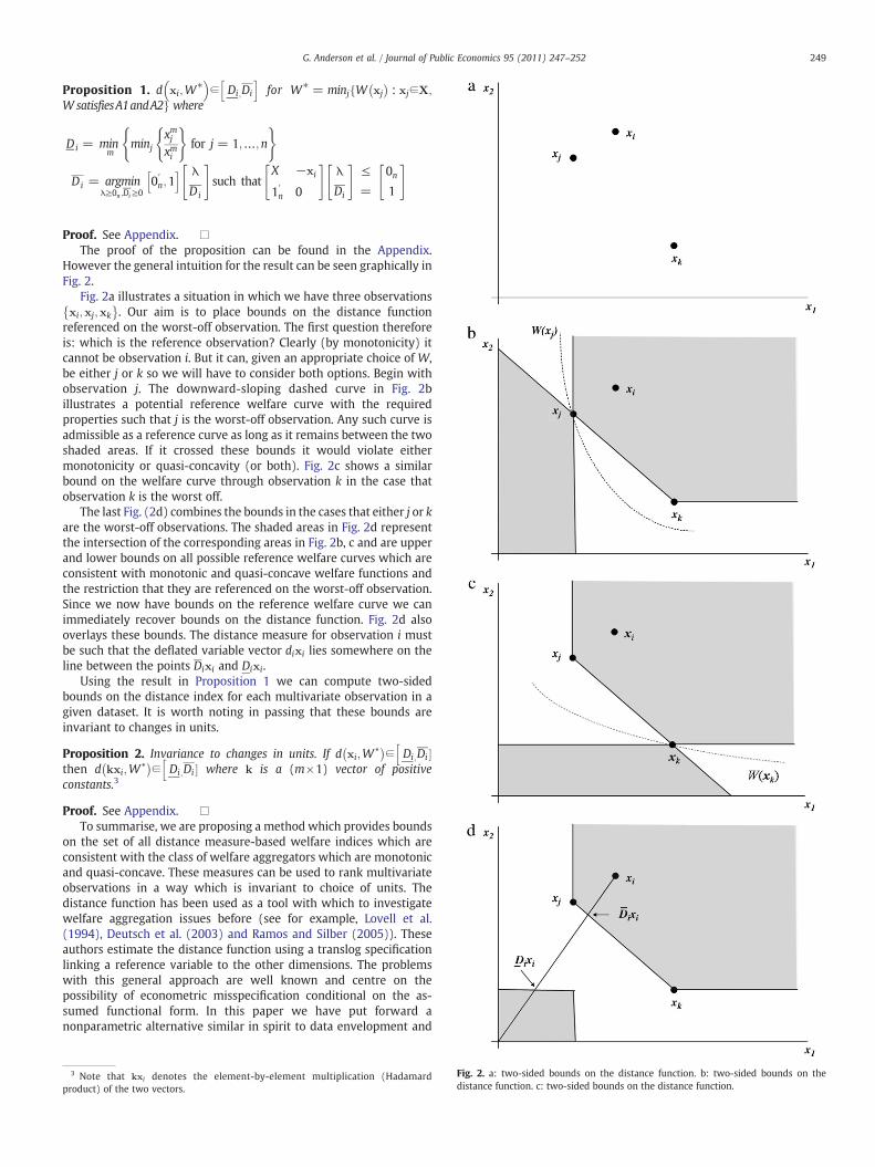
Proposition 1. d xi;W�� �

∈PDi ;Di

h ifor W� = minjfW xj

� �: xj∈X;

WsatisfiesA1andA2g where

PDi = minm

minjxmjxmi

( )for j = 1;…;n

( )

Di = argminλ≥0n ;Di≥0

0′n;1

h i λ

Di

" #such that

X −xi

1′n 0

" #λ

Di

" #≤=

0n

1

" #

Proof. See Appendix. □The proof of the proposition can be found in the Appendix.

However the general intuition for the result can be seen graphically inFig. 2.

Fig. 2a illustrates a situation in which we have three observationsxi;xj;xk

� �. Our aim is to place bounds on the distance function

referenced on the worst-off observation. The first question thereforeis: which is the reference observation? Clearly (by monotonicity) itcannot be observation i. But it can, given an appropriate choice of W,be either j or k so we will have to consider both options. Begin withobservation j. The downward-sloping dashed curve in Fig. 2billustrates a potential reference welfare curve with the requiredproperties such that j is the worst-off observation. Any such curve isadmissible as a reference curve as long as it remains between the twoshaded areas. If it crossed these bounds it would violate eithermonotonicity or quasi-concavity (or both). Fig. 2c shows a similarbound on the welfare curve through observation k in the case thatobservation k is the worst off.

The last Fig. (2d) combines the bounds in the cases that either j or kare the worst-off observations. The shaded areas in Fig. 2d representthe intersection of the corresponding areas in Fig. 2b, c and are upperand lower bounds on all possible reference welfare curves which areconsistent with monotonic and quasi-concave welfare functions andthe restriction that they are referenced on the worst-off observation.Since we now have bounds on the reference welfare curve we canimmediately recover bounds on the distance function. Fig. 2d alsooverlays these bounds. The distance measure for observation i mustbe such that the deflated variable vector dixi lies somewhere on theline between the points Dixi and Dixi.

Using the result in Proposition 1 we can compute two-sidedbounds on the distance index for each multivariate observation in agiven dataset. It is worth noting in passing that these bounds areinvariant to changes in units.

Proposition 2. Invariance to changes in units. If d xi;W T� �

∈PDi ;Di �

hthen d kxi;W T

� �∈

PDi ;Di �

hwhere k is a (m×1) vector of positive

constants.3

Proof. See Appendix. □To summarise, we are proposing a method which provides bounds

on the set of all distance measure-based welfare indices which areconsistent with the class of welfare aggregators which are monotonicand quasi-concave. These measures can be used to rank multivariateobservations in a way which is invariant to choice of units. Thedistance function has been used as a tool with which to investigatewelfare aggregation issues before (see for example, Lovell et al.(1994), Deutsch et al. (2003) and Ramos and Silber (2005)). Theseauthors estimate the distance function using a translog specificationlinking a reference variable to the other dimensions. The problemswith this general approach are well known and centre on thepossibility of econometric misspecification conditional on the as-sumed functional form. In this paper we have put forward anonparametric alternative similar in spirit to data envelopment and

3 Note that kxi denotes the element-by-element multiplication (Hadamardproduct) of the two vectors.

Fig. 2. a: two-sided bounds on the distance function. b: two-sided bounds on thedistance function. c: two-sided bounds on the distance function.

250 G. Anderson et al. / Journal of Public Economics 95 (2011) 247–252

revealed preference approaches. The main difference from dataenvelopment analysis is that whilst in a standard envelopmentproblem both inputs and outputs are observed, we only observeinputs. We use restrictions on the class of admissible planners'aggregation functions (monotonicity and quasi-concavity) and aparticular choice of reference observation (the worst off) to allowus to get around this problem. The main weakness of this type ofapproach is similar to the problems of standard envelopmentproblems: the results are data-dependent and so can sometimes beinfluenced by outliers and may consequently be determined byrelatively few, extreme (low) observations.

3. An empirical illustration: international development

We focus on a now well-established measure of internationaldevelopment produced by the United Nations, the Human Develop-ment Index (HDI). Data was taken from the UNDP (2009) HumanDevelopment Report 2009, which measures information for the year2007 on 182 nations.4 There are three indicators of well-being — lifeexpectancy at birth in years, education (measured as a combination ofindicators of adult literacy and the combined enrolment rate in alllevels of education), and GDP per capita, measured in US dollars atpurchasing power parity. The HDI is calculated by comparing thevalue of each indicator to benchmark upper and lower levels. Thisproduces three indices between zero and one which represent theextent to which a country has moved towards the upper benchmark.For example, the life expectancy benchmarks are 25 years and85 years. A country with a life expectancy of 25 years or lowerwould get an index of zero; a country with a life expectancy of85 years or more receives an index of one. In 2007, the UK's lifeexpectancy was 79.3 years which gave it a life expectancy index of thefollowing: 79:3−25

85−25 = 0:906. The overall HDI is a simple average of thelife expectancy, education and GDP indices. Our distancemeasures arecalculated from the three component indices used in the HDI. It isimportant to recognise that, like the HDI, we do not consider thedynamic interrelationship between the indicators. For example, onemight think of higher levels of education as generating higher GDP inthe future. Similarly, higher GDP/capita would be associated withhigher longevity. While there may be some more complex relation-ships associated with the distribution of GDP or the distribution ofeducation across the population, these are not addressed in thispaper.5

As discussed in the introduction, the HDI is an existing example ofattempts to combine multiple indicators of well-being into a singleindex and highlights clearly many of the issues in doing so. Evenassuming that the indicators are measured reliably and comparablyacross countries, and each index is meaningful in itself (capping themaximum possible life expectancy at 85 means, for example, that acountry with a life expectancy of 100 would be no more ‘developed’than onewith a life expectancy of 856), assigning equal weight to eachis clearly arbitrary. Analysis from the 2008 update of the HDI figures(UNDP, 2008) suggested that “… 70 percent of all possible country-pair comparisons are fully robust, meaning that the rankings wouldnot be reversed at any non-negative weights that sum to 1.” This, ofcourse, reflects all possible pairwise comparisons and it is hard toimagine that countries at the top of the index would ever fall belowthose at the bottom on any re-weighting of the data. We may expectmuch more fluctuation in the ranks of countries close to one another.

4 Source data is available from http://hdr.undp.org/en/media/HDR_2009_Tables.xls.5 We are grateful to an anonymous referee for suggesting this line of future research.6 For the income index, the upper limit is set at $40,000 per capita at PPP. Thirteen of

the 182 countries studied had incomes above this value meaning that Liechtenstein,with an income of $85,382 per capita, has the same GDP index as Switzerland despitethe latter's income per capita being half as much ($40,658 per capita).

The report does point out that “… at some parts of the distribution,including among the top ten countries… the rankings are sensitive tochanges in the weights of the underlying components.”

We took the data published in theHumanDevelopment Report 2009and computed, for each country, bounds on the distance index asdescribed in the previous section. Fig. 3 shows the countries orderedfromworst-off to best-off according to the mid-point of their distancebounds, along with the lower and upper bounds. Recall that highervalues of the distance measure represent lower welfare. For ease ofexposition, we have subtracted the bounds from 1 such that highervalues reflect higher welfare. The results indicate that the bounds onthe distance measure are informative about welfare comparisonsacross countries: the bounds do not span the entire interval [0,1] andon average across all countries, the gap between upper and lowerbound is 0.246. Using the mid-point of the bound to rank countries,the best-off nation is Norway, which has an interval [0.637,0.818]. Ofthe 182 nations in the HDI, 38 have bounds that do not overlap theNorwegian bounds at all. Similarly, ranking by the mid-point theworst-off country is Niger, with bounds [0.000,0.407]. In total, 132countries have bounds that do not overlap those of Niger.

In general, the size of the interval of the bounds is decreasing inoverall welfare. Particularly noticeable is that the bounds are typicallynarrowest for better-off nations. Of the 68 countries with a mid-pointbelow 0.6, the average width of the bounds is 0.330 whilst the 114countries with a mid-point in excess of 0.6 have an average width of0.196. The largest interval is Swaziland ([0.086,0.718]) and thenarrowest interval is Vietnam ([0.507,0.665]). Conceptually, both theoverall magnitude of the welfare inputs and their variability may beimportant determinants of the width of the bound. The correlationcoefficient between the interval width and the mean of the lifeexpectancy, education and GDP indices is −0.801 which mirrors theresult from Fig. 3 that better-off nations have tighter bounds. Thecorrelation coefficient between the interval width and the standarddeviation of the indices is +0.401, suggesting countries with morevariable inputs tend to have wider bounds.

The Human Development Report classifies countries with an HDI inexcess of 0.9 as “very high human development”, countries with anHDI between 0.8 and 0.9 as “high human development”, countrieswith an HDI between 0.5 and 0.8 as “medium human development”and countries with an HDI below 0.5 as “low human development”.Fig. 4 re-orders countries according to their HDI (worst-off on theleft), demarcating these different development rankings, and showsthe distance bounds as above.

Clearly there is a close relationship between HDI and the distancemeasures suggesting the particular choice of aggregation method inthe HDI is quite robust. The variation in the bounds for countriesclassed as ‘very high development’ is particularly small. However it isclear that there is some overlap between the groups. Taking the mid-point of the bounds as a welfare measure, 4 of the 38 countries ranked

Fig. 3. Welfare bounds.

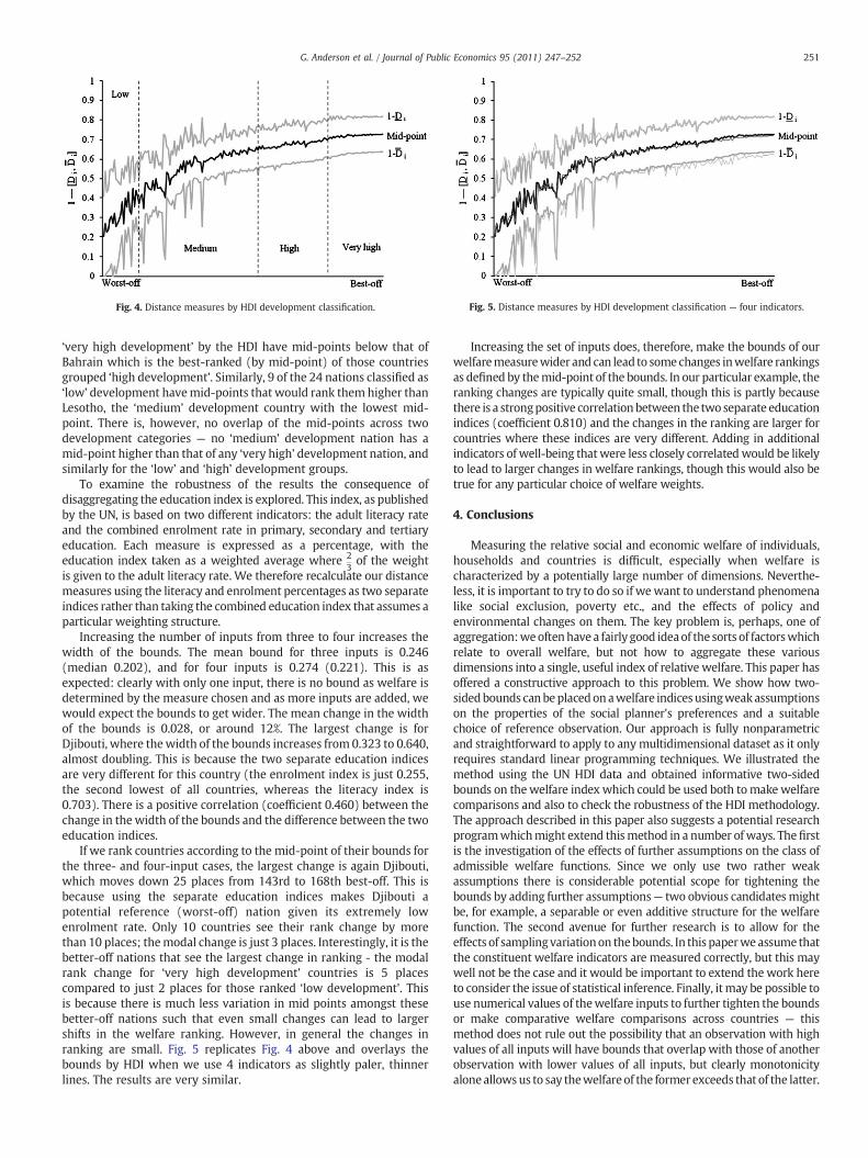
Fig. 5. Distance measures by HDI development classification — four indicators.Fig. 4. Distance measures by HDI development classification.

251G. Anderson et al. / Journal of Public Economics 95 (2011) 247–252

‘very high development’ by the HDI have mid-points below that ofBahrain which is the best-ranked (by mid-point) of those countriesgrouped ‘high development’. Similarly, 9 of the 24 nations classified as‘low’ development havemid-points that would rank them higher thanLesotho, the ‘medium’ development country with the lowest mid-point. There is, however, no overlap of the mid-points across twodevelopment categories — no ‘medium’ development nation has amid-point higher than that of any ‘very high’ development nation, andsimilarly for the ‘low’ and ‘high’ development groups.

To examine the robustness of the results the consequence ofdisaggregating the education index is explored. This index, as publishedby the UN, is based on two different indicators: the adult literacy rateand the combined enrolment rate in primary, secondary and tertiaryeducation. Each measure is expressed as a percentage, with theeducation index taken as a weighted average where 2

3of the weight

is given to the adult literacy rate. We therefore recalculate our distancemeasures using the literacy and enrolment percentages as two separateindices rather than taking the combined education index that assumes aparticular weighting structure.

Increasing the number of inputs from three to four increases thewidth of the bounds. The mean bound for three inputs is 0.246(median 0.202), and for four inputs is 0.274 (0.221). This is asexpected: clearly with only one input, there is no bound as welfare isdetermined by the measure chosen and as more inputs are added, wewould expect the bounds to get wider. The mean change in the widthof the bounds is 0.028, or around 12%. The largest change is forDjibouti, where thewidth of the bounds increases from 0.323 to 0.640,almost doubling. This is because the two separate education indicesare very different for this country (the enrolment index is just 0.255,the second lowest of all countries, whereas the literacy index is0.703). There is a positive correlation (coefficient 0.460) between thechange in thewidth of the bounds and the difference between the twoeducation indices.

If we rank countries according to the mid-point of their bounds forthe three- and four-input cases, the largest change is again Djibouti,which moves down 25 places from 143rd to 168th best-off. This isbecause using the separate education indices makes Djibouti apotential reference (worst-off) nation given its extremely lowenrolment rate. Only 10 countries see their rank change by morethan 10 places; themodal change is just 3 places. Interestingly, it is thebetter-off nations that see the largest change in ranking - the modalrank change for ‘very high development’ countries is 5 placescompared to just 2 places for those ranked ‘low development’. Thisis because there is much less variation in mid points amongst thesebetter-off nations such that even small changes can lead to largershifts in the welfare ranking. However, in general the changes inranking are small. Fig. 5 replicates Fig. 4 above and overlays thebounds by HDI when we use 4 indicators as slightly paler, thinnerlines. The results are very similar.

Increasing the set of inputs does, therefore, make the bounds of ourwelfaremeasurewider and can lead to somechanges inwelfare rankingsas defined by themid-point of the bounds. In our particular example, theranking changes are typically quite small, though this is partly becausethere is a strongpositive correlationbetween the twoseparate educationindices (coefficient 0.810) and the changes in the ranking are larger forcountries where these indices are very different. Adding in additionalindicators of well-being thatwere less closely correlatedwould be likelyto lead to larger changes in welfare rankings, though this would also betrue for any particular choice of welfare weights.

4. Conclusions

Measuring the relative social and economic welfare of individuals,households and countries is difficult, especially when welfare ischaracterized by a potentially large number of dimensions. Neverthe-less, it is important to try to do so if wewant to understand phenomenalike social exclusion, poverty etc., and the effects of policy andenvironmental changes on them. The key problem is, perhaps, one ofaggregation:weoftenhave a fairly good ideaof the sorts of factorswhichrelate to overall welfare, but not how to aggregate these variousdimensions into a single, useful index of relative welfare. This paper hasoffered a constructive approach to this problem. We show how two-sidedbounds canbeplacedonawelfare indicesusingweakassumptionson the properties of the social planner's preferences and a suitablechoice of reference observation. Our approach is fully nonparametricand straightforward to apply to any multidimensional dataset as it onlyrequires standard linear programming techniques. We illustrated themethod using the UN HDI data and obtained informative two-sidedbounds on thewelfare index which could be used both tomake welfarecomparisons and also to check the robustness of the HDI methodology.The approach described in this paper also suggests a potential researchprogramwhichmight extend thismethod in a number ofways. Thefirstis the investigation of the effects of further assumptions on the class ofadmissible welfare functions. Since we only use two rather weakassumptions there is considerable potential scope for tightening thebounds by adding further assumptions— two obvious candidatesmightbe, for example, a separable or even additive structure for the welfarefunction. The second avenue for further research is to allow for theeffects of samplingvariationon thebounds. In this paperweassume thatthe constituent welfare indicators are measured correctly, but this maywell not be the case and it would be important to extend the work hereto consider the issue of statistical inference. Finally, itmay be possible touse numerical values of thewelfare inputs to further tighten the boundsor make comparative welfare comparisons across countries — thismethod does not rule out the possibility that an observation with highvalues of all inputs will have bounds that overlap with those of anotherobservation with lower values of all inputs, but clearly monotonicityaloneallowsus to say thewelfareof the former exceeds that of the latter.

252 G. Anderson et al. / Journal of Public Economics 95 (2011) 247–252

Acknowledgments

We would like to thank Ian Preston and Martin Ravallion for theirhelpful discussions and comments. Financial support from the ESRCgrant number RES-000-22-0393 is gratefully acknowledged. Theauthors are responsible for all errors.

Appendix. Proofs

Proof of Proposition 1. Consider the upper bound. Let λ and Di

denote the solutions to the linear programme given in the definitionof Di . Now suppose that d xi;W T

� �N Di . Since λ≥0n, 1′nλ=1 and

Dixi = Xλ, we have W Dixi� �

= W Xλð Þ≥W T = minj W xj� �

xj∈X� �

for all aggregators satisfying A→ and A2. Therefore, if d xi;W T� �

N Di ,then W d xi;W T

� �xi

� �N W Dixi

� �which implies that d xi;W T

� �N

mind≥0 d : W dxið Þ≥W T� �

which contradicts the definition of thedistance function. Now consider the lower bound and suppose that

PDi Nd xi;W T� �

. This implies that minm d xi;W T� �

xmi� �

bminmfminj xmjn o

for j=1,...,n} whereminm{minj{xjm} for j=1,...,n}=W * for the Leontiefaggregator function (which satisfies A1 and A2) and hence thatW d xi;W T

� �xi

� �bW T which contradicts the definition of the distance

function. □

Proof of Proposition 2. Consider the lower bound and note that xjm /xim=kmxj

m /kmxim so invariance follows immediately. Now consider theupper bound and suppose that Di solves the linear program describedin Theorem 1. Then Dixi = Xλ and hence Di also satisfiesDi kxi½ � = kX½ �λ. □

References

Anand, S., Sen, A.K., 1997. Concepts of human development and poverty: amultidimensional perspective. Human Development Papers. UNDP, New York.

Atkinson, A.B., 2003. Multidimensional deprivation: contrasting social welfare andcounting approaches. Journal of Economic Inequality 1 (1), 51–65.

Bourguignon, F., Chakravarty, S.R., 2003. The measurement of multidimensionalpoverty. Journal of Economic Inequality 1 (1), 25–49.

Deaton,A., 1979. Thedistance function in consumerbehaviourwith anapplication to indexnumbers and optimal taxation. The Review of Economic Studies 46 (3), 391–405.

Deaton, A., Muellbauer, J., 1980. Economics and consumer behavior. CambridgeUniversity Press, Cambridge.

Deutsch, J., Ramos, X., Silber, J., 2003. Poverty and inequality of standard of living andquality of life in great britain. In: Sirgy, J., Rahtz, D., Samli, A.C. (Eds.), Advances inQuality-of-Life Theory and Research. Kluwer Academic Publishers, Dordrecht,pp. 99–128.

Grusky, D.B., Kanbur, R., 2006. Poverty and inequality: studies in social inequality.Stanford University Press, Stanford.

Kolm, S.C., 1977. Multidimensional egalitarianisms. Quarterly Journal of Economics 91(1), 1–13.

Lovell, C.A.K., Richardson, S., Travers, P., Wood, L., 1994. Resources and functionings: anew view of inequality in Australia. In: Eichhorn, W. (Ed.), Models andMeasurement of Welfare and Inequality. Springer-Verlag, Heidelberg.

Maasoumi, E., 1986. The measurement and decomposition of multidimensionalinequality. Econometrica 54 (4), 771–779.

Malmquist, S., 1953. Index numbers and indifference surfaces. Trabajos de Estadistica 4,209–242.

Ramos, X., Silber, J., 2005. On the application of efficiency analysis to the study of thedimensions of human development. Review of Income and Wealth 51 (2),285–309.

Rockafellar, R.T., 1970. Convex Analysis. Princeton University Press, Princeton.Sen, A.K., 1995. Inequality Reexamined. Harvard University Press, Harvard.Shephard, R.W., 1953. Cost and production functions. Princeton University Press,

Princeton.United Nations Development Programme, 2008. Human Development Indices: A

statistical update 2008. UNDP, New York.United Nations Development Programme, 2009. Human Development Report 2009 —

overcoming barriers: human mobility and development. UNHDP, New York.