WORKING PAPER #468 PRINCETON UNIVERSITY INDUSTRIAL RELATIONS SECTION JULY 2002 http://www.irs.princeton.edu/pubs/working_papers.html

What Are Food Stamps Worth?

Diane Whitmore Industrial Relations Section

Firestone Library Princeton University Princeton, NJ 08544

whitmore@princeton.edu

July 31, 2002

I thank Orley Ashenfelter, David Autor, Anne Case, Melissa Clark, Angus Deaton, Erica Field, Jeff Kling, Alan Krueger, Phil Levine, David Linsenmeier, Doug Miller, Peter Orszag, Anu Rangarajan, Cecilia Rouse, Aaron Sparrow, Liz Stuart and Mark Votruba and the participants in the Princeton Labor Lunch for extremely helpful comments. I also thank Ed Freeland, Jim Ohls, David Super and Parke Wilde for useful discussions and their generosity in providing data, and Brian Feinstein, Ishani Ganguli and Neil Kadagatur for research assistance. Financial support from the Industrial Relations Section, the National Science Foundation, and the Woodrow Wilson Society of Fellows is gratefully acknowledged.

2

What Are Food Stamps Worth?

Abstract

The carte-blanche principle implies that food stamp recipients would be better off if they were given cash instead of an equivalent amount in food stamps. I estimate the cash-equivalent value of food stamps and the lowest price a recipient would accept to sell her “extra” food stamps on the underground market. I estimate that between 20 and 30 percent of food stamp recipients spend less on food than their food stamp benefit amount if they receive cash instead of stamps, and therefore would be better off with cash. Using a theoretical model I present and data from experiments conducted in two states, I estimate that on average “distorted” food stamp recipients value their total benefits at 80 percent of their face value. Aggregating over recipients, the annual deadweight loss associated with the food stamp program is one-half billion dollars. Food diary data indicate that providing cash instead of stamps causes some distorted recipients to decrease their food spending – especially on soda and juice – but has no negative consequence for nutrition. As predicted by theory, inframarginal food stamp recipients do not alter their behavior if they are given cash instead of food stamps. Although paying in-kind benefits results in some deadweight loss, it is thought that an underground market for the excess stamps will be created to alleviate some of the loss. I present new survey evidence indicating that stamps trade for only about 65 percent of their face value on the underground market. Diane Whitmore Industrial Relations Section Firestone Library Princeton University Princeton, NJ 08544 whitmore@princeton.edu

3

I. Introduction

According to the carte blanche principle in economics, a consumer is (weakly) better off

if she is given cash than if she is paid an in-kind transfer. As long as the consumer is rational,

the ability to choose how to optimize her budget over all goods will allow her to attain a level of

utility at least as high or higher than when part of the budget is restricted to purchase only certain

goods. A canonical example taught in Econ 101 to illustrate this concept is the effect of food

stamps on consumer spending in a model with a budget constraint and utility curve. Simply put,

the model says that if you give someone $100 in food stamps, one of two things will happen. If

the person would have otherwise spent more than $100 on food, then she will treat the food

stamps just like cash (and is termed “inframarginal”). But if the person would have spent less

than $100 on food otherwise, then the food stamps will cause her to shift her spending and

consume more food so she can use the stamps – that is, the food stamps will distort her choices,

and her utility will be maximized at the corner solution. (Throughout the paper, consumers in

this case will be referred to as “distorted”.) This results in deadweight loss.

To some, this distortion is the best part of the food stamp program: the government can

ensure that needy families get enough to eat and that they don’t spend the money on other things.

To others, this distortion represents a waste of resources – it is inefficient to give in-kind

transfers instead of cash.1

How much efficiency is lost from paying food stamps in-kind instead of in cash? In

order to measure the deadweight loss to food stamp recipients, I develop a method to estimate

the cash-equivalent value of food stamps based on the price elasticity of food and the magnitude

1 See, for example, Doug Besharov’s comments in the November 14, 2001 New York Times, p. A14. He argues: “in some instances, particularly the elderly, they might need money to pay utility bills, rather than more food stamps.”

4

of the food-stamp-induced consumption distortion.2 I apply this method using experimental data

and find the cash-equivalent value of food stamps to be about 80 cents per dollar. Using this

estimate, I calculate an annual deadweight loss of over one-half billion dollars – or 3 percent of

the benefit expenditures. When the extra cost savings of administering the food stamp program

through check payments and savings to retailers are added in, the potential total annual savings

nears $1 billion.

Despite the inefficient use of resources, issuing food stamps may still be a good public

policy. For example, the receipt of food stamps – instead of cash – may cause participants to eat

a nutritionally superior diet. To examine this question, I use two field experiments in which

some food stamp recipients were randomly selected to receive cash instead of food stamps. With

these data, I test the effect of paying benefits in food stamps instead of cash on food

consumption, nutritional intake, and spending on other budget items. I find small and

insignificant changes in the intake of individual commodities and nutrients in most cases. I find

evidence that nutrition may actually improve when benefits are paid in cash, as extreme over-

consumption of calories and junk food intake decline.

I extend the theory to predict the lowest price a distorted food stamp recipient would

accept to sell her “extra” benefits. In addition, I present original survey evidence on the price for

which food stamps are traded on the underground market. These results suggest food stamps

trade for about 61 cents per dollar.

I find that the government could save over one-half billion dollars per year if it paid food

stamp benefits in a cash transfer equal to their value to recipients, and if it paid benefits in cash

the nutrient intake of recipients would not decline. Nonetheless, there still may be other political

2 Throughout, I use cash-equivalent value to refer to the average, not marginal, value of the entire food stamp transfer to the recipient. Later, I also present estimates of the value of “extra” food stamps.

5

reasons to retain the status quo. Unlike most cash-welfare programs, food stamps enjoy

tremendous public support that might erode if benefits were no longer directly linked to food

purchases.3 As a result, the deadweight loss and excess administrative expenditures of

$0.5-1.0 billion per year may be a price worth paying to retain strong program support.

II. Background on the Underground Market for Food Stamps

The deadweight loss from food stamps occurs only to the extent that recipients cannot

undo the spending distortion by selling their unwanted food stamps at or near face value.

Evidence suggests that there is an active underground market for food stamps. Some recipients

sell all or part of their benefits, which alleviates some of the deadweight loss that would

otherwise occur (Edin and Lein, p. 41). But the price of benefits is not bid up to nearly their face

value. As shown below, benefits are typically sold on the underground market for about

61 percent of their face value.

One possible reason that stamps trade at significantly below their face value is that

trading benefits is illegal, so some buyers and sellers might refrain from participating in the

market. For those who do participate in the market, the search costs appear to be high. It takes

significant matching effort to bring a willing buyer and seller together. Ten years ago, food

stamps could be sold to – or used to buy non-food items at – stores with merchants willing to

traffic benefits. But since the implementation of EBT (the Electronic Benefit Transfer system, in

which benefits are paid out using a rechargeable card similar to a debit card), large-scale

trafficking by merchants is relatively easy to track. Now it appears that most trafficking takes

3 Robert Greenstein (1998) argues “cashing out [food stamps] would be exceedingly unwise” because if it were cashed out, the program would “likely be dismantled over time.” The trend in income-support programs has been to provide more in-kind transfers (such as health insurance) and benefits tied to certain desirable behaviors such as school attendance or work. Lawrence Mead terms these the “new paternalism” programs (Mead, 1997).

6

place with benefits sold to other individual shoppers in stores, or to friends or family.4 As a

result, it may take longer for sellers to find willing individuals to purchase all of the food stamps

they want to sell. There is also a risk of being caught; recipients caught selling their benefits can

be removed from the food stamp program, and buyers can be charged with a felony if caught

with $100 or more in illegally traded food stamps. Trafficking is typically done in small-stake

amounts, so sellers might be more willing to accept a slightly lower price instead of having to

search for a buyer willing to pay a higher price.

The extent of trafficking is not well known. The GAO reports that it cannot precisely

estimate the dollar value of food stamp trafficking, but suggests that the incidence of trafficking

is approximately 3.7 percent of annual benefits (or about $800 million) but may be as high as

10 percent of all food stamp benefits.5

Since stamps trade for a price significantly below their face value on the underground

market, there is still a deadweight loss associated with paying benefits in-kind instead of in cash.

In order to measure the magnitude of this loss, I will estimate the cash-equivalent value of food

stamps to the distorted consumers. First I turn to a review of the literature, and then I develop a

model to estimate the value of food stamps.

III. Literature on Cash-Equivalent Values

Others have estimated the cash-equivalent value of food stamps, but the earlier literature

is limited by methodology and data. Smeeding (1982) estimates the cash value of food stamps to

4 See survey results, below. 5 See U.S. General Accounting Office (1995), and Committee on Ways and Means (2000) p 882. These reports were written before benefit payment via electronic benefit transfer (EBT) was the norm. EBT is thought to make it more difficult to traffic food stamps, especially for retailers. Pilot projects in New Mexico and Minnesota found a 75–81 percent reduction in fraud due to the introduction of EBT (OVP, 1993). Macaluso (2000) finds that expansion of EBT helped contribute to the 19 percent decrease in trafficking between 1993 and 1998.

7

be 97 percent of the face value by comparing food expenditures of food stamp recipients to

program non-participants with the same income.6 If there are unobservable differences between

the groups that affect both food spending and the decision to participate in the food stamp

program, though, this type of comparison will give biased results.7

In 1982, the entire Puerto Rican food stamp program began to be paid in cash instead of

stamps, but there was no measurable impact on food spending when benefits were converted to

cash. Moffitt (1989) estimates a piecewise-linear constraint model to determine why there was

no cash-out effect, and concludes that the stamps were valued at 100 percent of their face value

even before the cash-out. One possible explanation for this is that, since Puerto Rican benefit

levels are low relative to income, most consumers were inframarginal.8 Moffitt also finds

indirect evidence of a high incidence of trafficking that may have increased the value of stamps

to recipients who were not inframarginal, and reduced the effect of the cash-out. Although

Moffitt’s analysis is convincing, the results from Puerto Rico may not be generalizable to the

contiguous United States.

Since my estimates of the cash-equivalent value of food stamps are based on unique

experimental data, unlike some of the earlier work, my results will not be plagued by differences

in unobservables between program participants and non-participants. Furthermore, unlike the

food stamp recipients in Puerto Rico, the participants in the cash-out experiments analyzed in my 6 Literature prior to the elimination of the purchase requirement in 1979 (summarized in Smeeding, 1982) estimates the overall cash-equivalent value to be between 83 and 96 percent of face value. Cooper and Katz (cited in Moffitt, 1989) estimate (based on simulations) that very low-income households value their food stamps as low as 39 percent of face value. The earlier literature is not directly relevant because the elimination of the purchase requirement altered the value of food stamps to recipients. The purchase requirement required recipients to pay a price below their face value to receive food stamps. For example, a family may have been charged $50 to receive $150 in food stamps. Today the same family would be offered a $100 take-it-or-leave-it food stamp benefit with no cost outlay on their part. 7 Daponte, Sanders and Taylor (1999) find that many low-income households that do not participate in the food stamp program have substantially more wealth than participants, suggesting underlying differences between the groups. 8 Only 8 percent of the Puerto Rico sample is estimated to spend the same or less on food than their food stamp benefit.

8

study have characteristics that are reasonably similar to those of U.S. food stamp recipients as a

whole (as shown in Table 1, below).

IV. Measuring the Cash-Equivalent Value of Food Stamps

In order to estimate the deadweight loss from food stamps, I must estimate the cash-

equivalent value of food stamps. For inframarginal consumers, as implied by theory, the value is

assumed to be the face value of the benefits. As shown below, the empirical results are

consistent with this assumption; when given cash instead of food stamps, inframarginal

consumers do not change their purchasing patterns. Below I present a method to estimate the

value of food stamps to consumers who are not inframarginal.

In this section, I use a utility maximization framework to develop a model to estimate the

cash-equivalent value of food stamps to distorted consumers. Consider first a consumer who

receives her food stamp benefits in cash. She has a choice between two goods: food (x1) and

other goods (x2) with fixed prices (p1 and p2). The consumer has income (y), which in this case

comprises a cash grant from the government (y1) and other income (y2). She chooses

consumption levels subject to her budget constraint to maximize utility. Utility maximization

leads to commodity demand functions:

1 2( , , )i ix x p p y=

for i = (1, 2). The commodity demand functions are substituted into the utility function

1 2( , )u u x x= to get the following indirect utility function:

* *1 2( , , )p p yυ υ= .

Solve the indirect utility function for income:

*1 2( , , )y E p p υ= . (0.1)

9

The resulting equation is the minimum (unearned) income necessary to obtain utility level *υ ,

and can be thought of as the excess expenditure function.

Introducing Food Stamps

Now introduce food stamps into the model. Instead of receiving a cash grant from the

government, a consumer receives an income transfer of the same amount in food stamp benefits

( f ) that can only be used to purchase food. The amount of food that can be purchased using

solely food stamps is 1x , such that 1 1f x p= . Income (y) comprises the sum of food stamps ( f )

that can only be spent on food, and other income (y2, as above) that can be spent on either food

or other goods. Note that the level of y is the same in both cases, but in the first case y can be

spent on any combination of food and non-food, and in the second case an amount greater than

or equal to the food stamp benefit ( f ) must be spent on food.

As before, the consumer chooses consumption of commodities to maximize utility subject

to the budget constraint. In the case in which demand for food is at least as great as the minimal

amount that can be purchased using food stamps – that is, 1 1 2 1( , , )x p p y x≥ – utility is maximized

as usual and she is said to be inframarginal, or “non-distorted.”

In the case in which 1 1 2 1( , , )x p p y x< , the consumer’s non-distorted utility (holding y

fixed but not requiring f to be spent on food) would be maximized by consuming less food than

the minimal amount that could be bought with her food stamp benefit. Assuming strong

monotonicity, these consumers are “required” to consume 1x , which is a larger amount of food

than they would otherwise choose to consume. These consumers are said to have their

10

consumption pattern “distorted” by food stamp receipt. Such consumers maximize utility taking

the consumption level of food as given. The utility function is then:

1 2( , )u u x x=

subject to the budget constraint:

1 1 2 2y x p x p= + .

Maximization yields distorted consumers’ modified commodity demand function for other

goods:

2 2 1 2 1 1( , , )x x x p y x p= − .

As before, substituting the modified commodity demands into the utility function:

1 2 1 2 1 1

1 2 1 1

[ , ( , , )]

( , , ).

u x x x p y x p

x p y x p

υυ

= −

= − (0.2)

A distorted consumer will have a welfare loss compared to a non-distorted consumer, so

*υ υ< . Solve equation (0.2) for the income y necessary to obtain utility level υ :

1 2 1 1( , , )y R x p x pυ= + . (0.3) Recall from above that *

1 2( , , )y E p p υ= is the amount of income necessary to obtain utility level

υ for a non-distorted consumer. Then the amount

* * *1 2 1 2 1 1 1 2( , , ) ( , , ) ( , , )C x p R x p x p E p pυ υ υ= + − (0.4)

is the lump-sum transfer payment necessary to raise the utility level of a consumer with her

choices distorted by food stamps to the (higher) utility level of a non-distorted consumer. The

amount

1 1

1 1

x p Cx p

θ −= (0.5)

11

measures the ratio of the cash-equivalent value of food stamps to the distorted consumers to the

face value of the food stamps. That is, if the government were to give distorted food stamp

recipients cash instead of stamps, it could make lump-sum payments of θ times the face value of

the stamps and the recipients would still attain the same utility level. Note that 1 1 1( )C p x x< − ;

the transfer required to elevate a consumer’s utility to the non-distorted level is smaller than the

price of the “extra” food consumed, since the distorted consumer gets some utility from the extra

food.

In order to estimate the cash-equivalent value of food stamps, one could impose a

functional form on the utility function and solve the indirect utility functions for the income

required to equalize utility in the distorted and non-distorted cases. Instead, I will proceed by

approximating C using a second-order Taylor series expansion of the lump-sum payment

equation (0.4) around the non-distorted equilibrium. At the non-distorted equilibrium, 1 1x x=

and

1 2 1 1 1 2( , , ) ( , , )R x p x p E p pυ υ+ = . (0.6)

Recall that the derivative of the excess expenditure function equals the compensated (Hicksian)

demand function:

1 2 1 2( , , ) ( , , )i ii

EE p p x p pp

υ υ∂= =∂

.

Substituting into the equilibrium condition (0.6) gives the following:

1 1 2 2 1 1 1 2 1 2( ( , , ), , ) ( , , ) ( , , )R E p p p p E p p E p pυ υ υ υ+ = . (0.7)

As an aside, here we can differentiate equation (0.7) with respect to 1p . This becomes helpful

below:

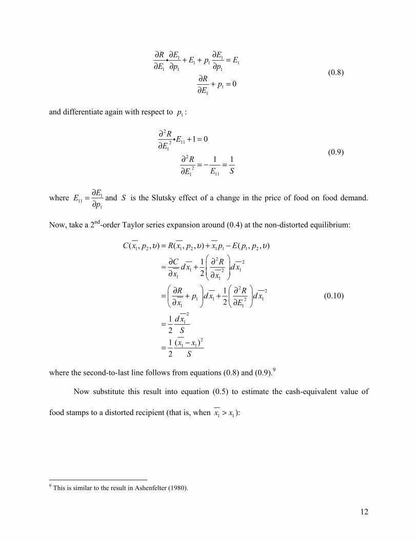
12

1 11 1 1

1 1 1

11

0

R E EE p EE p p

R pE

∂ ∂ ∂+ + =∂ ∂ ∂

∂ + =∂

i (0.8)

and differentiate again with respect to 1p :

2

1121

2

2111

1 0

1 1

R EE

RE SE

∂ + =∂

∂ = − =∂

i (0.9)

where 111

1

EEp

∂=∂

and S is the Slutsky effect of a change in the price of food on food demand.

Now, take a 2nd-order Taylor series expansion around (0.4) at the non-distorted equilibrium:

1 2 1 2 1 1 1 2

2 2

1 121 1

2 2

1 1 121 1

2

1

21 1

( , , ) ( , , ) ( , , )

12

12

121 ( )2

C x p R x p x p E p p

C Rd x d xx x

R Rp d x d xx E

d xSx x

S

υ υ υ= + −

∂ ∂ ≈ + ∂ ∂

∂ ∂= + + ∂ ∂

=

−=

(0.10)

where the second-to-last line follows from equations (0.8) and (0.9).9

Now substitute this result into equation (0.5) to estimate the cash-equivalent value of

food stamps to a distorted recipient (that is, when 1 1x x> ):

9 This is similar to the result in Ashenfelter (1980).

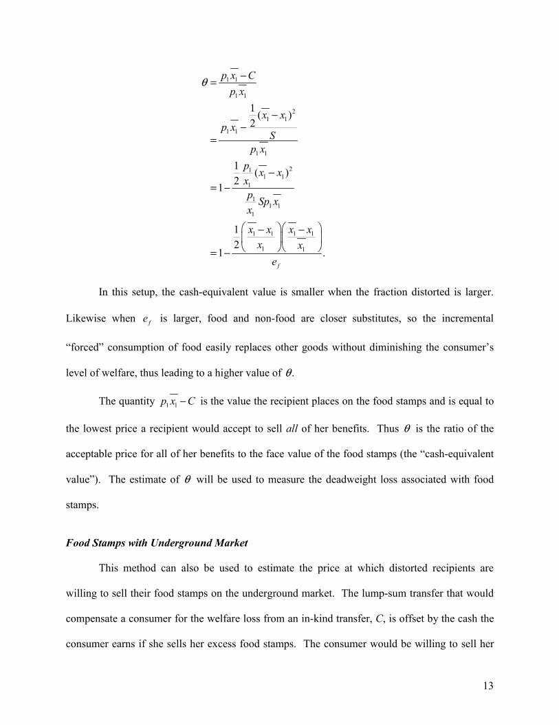
13

1 1

1 1

21 1

1 1

1 1

211 1

1

11 1

1

1 1 1 1

1 1

1 ( )2

1 ( )21

12

1 .f

p x Cp x

x xp x

Sp x

p x xxp Sp xx

x x x xx x

e

θ −=

−−

=

−= −

− − = −

In this setup, the cash-equivalent value is smaller when the fraction distorted is larger.

Likewise when fe is larger, food and non-food are closer substitutes, so the incremental

“forced” consumption of food easily replaces other goods without diminishing the consumer’s

level of welfare, thus leading to a higher value of .θ

The quantity 1 1p x C− is the value the recipient places on the food stamps and is equal to

the lowest price a recipient would accept to sell all of her benefits. Thus θ is the ratio of the

acceptable price for all of her benefits to the face value of the food stamps (the “cash-equivalent

value”). The estimate of θ will be used to measure the deadweight loss associated with food

stamps.

Food Stamps with Underground Market

This method can also be used to estimate the price at which distorted recipients are

willing to sell their food stamps on the underground market. The lump-sum transfer that would

compensate a consumer for the welfare loss from an in-kind transfer, C, is offset by the cash the

consumer earns if she sells her excess food stamps. The consumer would be willing to sell her

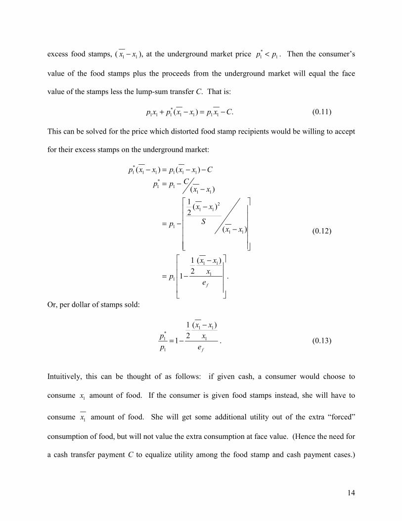
14

excess food stamps, ( 1 1x x− ), at the underground market price *1 1p p< . Then the consumer’s

value of the food stamps plus the proceeds from the underground market will equal the face

value of the stamps less the lump-sum transfer C. That is:

*1 1 1 1 1 1 1( ) .p x p x x p x C+ − = − (0.11)

This can be solved for the price which distorted food stamp recipients would be willing to accept

for their excess stamps on the underground market:

*1 1 1 1 1 1

*1 1

1 1

21 1

11 1

1 1

11

( ) ( )

( )1 ( )2

( )

1 ( )21 .

f

p x x p x x CCp p

x x

x x

Spx x

x xxp

e

− = − −

= −−

−

= − −

− = −

(0.12)

Or, per dollar of stamps sold:

1 1*1 1

1

1 ( )21

f

x xp xp e

−

= − . (0.13)

Intuitively, this can be thought of as follows: if given cash, a consumer would choose to

consume 1x amount of food. If the consumer is given food stamps instead, she will have to

consume 1x amount of food. She will get some additional utility out of the extra “forced”

consumption of food, but will not value the extra consumption at face value. (Hence the need for

a cash transfer payment C to equalize utility among the food stamp and cash payment cases.)

15

The distorted recipients should be willing to sell their excess food stamps for the dollar value of

the utility gained from the “forced” excess food consumption. A recipient who gets virtually no

utility from the extra consumption should be willing to sell her excess benefits for a small

amount, whereas a less distorted recipient would only be willing to sell her excess benefits at a

price closer to the face value.

Below, I will estimate *1p based on estimates of the parameters and present direct

evidence on the underground market price based on a telephone survey of food stamp recipients.

To estimate the cash-equivalent value of food stamps (θ ) and willing-to-accept price

( *1p ) based on the above setup, I use estimates of the compensated price elasticity of food ( fe )

and the difference between distorted and non-distorted food consumption ( )1 1x x− .

The next two sections obtain estimates for these parameters. Previous measures of the

magnitude of food stamps’ distortion on food consumption have been plagued by the typical

troubles associated with non-experimental estimates. For example, some studies compare food

consumption between low-income households who receive food stamps to those that do not,

without accounting for underlying differences that cause one group of families to select into the

program. Below I use experimental data to estimate the direct effect of food stamps on food

consumption for households that are not inframarginal.

V. Estimating Distortion Parameters

I will gauge the magnitude of food-stamp-induced distortion using a pair of experiments

from San Diego and Alabama that were implemented in the early 1990s by the U.S. Department

16

of Agriculture and originally evaluated by Mathematica Policy Research (MPR).10 In these so-

called “cash-out” experiments, food stamp benefits were paid out in cash to a random subset of

recipients instead of the then-typical food stamp coupons. The experiments were intended to

address a long-standing debate about how to best pay out food stamp benefits. In the San Diego

experiment the entire caseload was scheduled to have its food stamp benefits cashed-out for at

least 5 years; for evaluation purposes, 20 percent of the caseload was randomly chosen to receive

the cash-out 14 months early. In Alabama, the experiment was more limited: a random 4 percent

of the caseload in 12 rural and 2 urban counties had their benefits cashed-out for 8 months. At

the end of the 8-month trial, the experimental group was returned to traditional food stamp

payments.11 In the original MPR evaluations no attempt was made to divide the recipients into

distorted and non-distorted groups; their analysis was limited to a straightforward comparison of

cash vs. stamp recipients.

The survey response rate is linked to treatment status in Alabama: 76 percent of stamp

recipients vs. 80 percent of check recipients responded to the survey (p=0.008). Even though the

initial treatment assignment was random, this difference in response rates may introduce

selection bias. To account for this, I predict the propensity score using the method outlined in

Dehejia and Wahba (1998), and construct a dataset based on matched treatment and control

observations.12 As a result of the combination of the limited duration of the Alabama food stamp

10 There were two other cash-out experiments around the same time, another in Alabama and one in Washington State, but they were performed in conjunction with other changes in the states’ welfare programs. I will limit my analysis to the two “pure” cash-out experiments. Later, when welfare waivers were being widely granted by the Clinton Administration, over half of the states were granted limited cash-out of food stamps as part of their Section 1115 welfare waiver. PRWORA (the 1996 welfare reform law) prohibited any future cash-out of food stamps. 11 Observations were excluded if reported food spending was more than 75 percent of the household’s total income (including food stamp income). 12 The match was done with replacement. This method balances treatment and control samples on covariates, but of course cannot guarantee that no unobservable differences exist. Thirty observations from the treatment group were excluded because there was not a close enough propensity score match. The response rate did not differ by treatment status in San Diego, so those data are not adjusted except in definition (4) of Table 2, for comparison.

17

cashout and the need for the propensity score adjustment to balance the treatment and control

samples, I put less weight on the results from Alabama than those from San Diego.13

In this paper, I analyze the effect of the treatment on choices by distorted and non-

distorted households. To do so, I must empirically determine which households’ choices were

distorted and then use the experimental design to measure the difference in consumption between

distorted households receiving checks and those receiving stamps.14 First, since I rely on the

experiment for my results, I present some evidence to validate the randomization.

Examining the Validity of the Experiments

One limitation in the experimental design was that no baseline survey was conducted.15

In its absence, one way to investigate whether randomization was done properly is to compare

characteristics that are not affected by the treatment. Table 1 displays some characteristics that

are plausibly orthogonal to the treatment. As discussed above, since the response rates differed

by treatment status in Alabama, the table displays sample characteristics of the propensity score

matched sample. There are no discernible differences in the racial makeup or age of respondents

between the treatments and controls at either site. It is worth noting that the Alabama sample is

on average almost 13 years older than the San Diego sample. The overall Alabama sample and

San Diego sample have a similar percentage of white recipients, but in Alabama almost all of the

13 Since the Alabama cash-out was scheduled to last only 8 months – and was evaluated after 5–6 months – the period may have been too short for recipients to fully adjust their consumption patterns. There were also reports that recipients who were selected to receive checks were strongly encouraged by their caseworkers to continue to spend their benefits on food. In some cases they were reportedly warned that since the cash food stamp benefits were intended for food, they “could be arrested” if they spent it on other items. This could attenuate the cash-out effect in Alabama. 14 I will use the term “distorted” to refer to those receiving checks or stamps that spend the same or less on food purchases as their food stamp benefits. Of this subset, only the stamp recipients’ choices are actually distorted since the check recipients are able to re-optimize. The check recipients in this category would have had their choices distorted by food stamps in the absence of the cash-out. 15 MPR explains that the decision to forego a baseline survey primarily resulted from the budgetary and time cost of designing a survey instrument and conducting interviews.

18

non-white recipients are African American, while in San Diego there is a sizeable Hispanic and

Asian population.

The next two categories of variables – educational attainment and marital status – could

potentially be contaminated by a treatment effect. Because the experimental evaluations were

conducted after the cash-out had been in effect for only between 5 and 12 months, however, it

seems unlikely that the cash-out contributed to many changes in either category. As the table

shows, there are no measurable differences between the treatment and control groups for any of

these variables. One exception is that check recipients in Alabama appear to be slightly more

likely to be divorced, however the marital status variables are not jointly significant. Although it

is possible that the treatment should have affected employment status more strongly than the

other characteristics, the employment variables show no differences as well. The Alabama

sample is much more likely to be employed or retired/disabled than the San Diego sample.

Finally, the family unit size in San Diego deserves some scrutiny. In the original

evaluation, MPR concluded that there was a slight but statistically significant difference in

household size between the treatment and control groups. MPR investigated this to see if it was

evidence that the randomization was employed incorrectly, but concluded that any difference in

household size was due to sampling variation and not to a flaw in randomization. As a result,

MPR devised weights to make the average household size the same across groups and used those

weights throughout their analysis. My analysis re-calculates the size of the Food Stamp Unit

(FSU) and the Food Consumption Unit (FCU).16 Based on my analysis, the difference between

treatments and controls in FSU, FCU, and household size is not statistically significant. As a

16 The respondent reports whether each household member is part of the FSU and/or the FCU. I count the number of positive responses in each category and use the result as the FSU and FCU size, respectively. MPR claims to use the same method. It is possible that the final public-use version of the data had some corrections to the FSU and FCU data that account for the differences.

19

result, I do not use weights as MPR did in its analysis, but the results are similar whether or not

the data are weighted. Any difference could also be attributed to a treatment effect.17

For comparison to the experimental samples, column (5) lists characteristics of the

overall food stamp caseload from the Food Stamp Quality Control data file for 1990. San Diego

has more Hispanic and Asian food stamp recipients, and fewer African-American and White

recipients, than the U.S. as a whole. San Diego recipients are younger, better educated, more

likely to be married, and live in slightly larger households than the overall food stamp recipient

population. The Alabama sample is more African-American, is older and less educated, and has

a slightly larger household size than the country as a whole. Alabama food stamp recipients are

more likely to be employed or retired than either the San Diego sample or the country overall.

Measuring Distortion

The first method I use to measure the consumption distortion induced by food stamps

compares the recipients’ reported monthly spending at food stores to their reported food stamp

benefit received.18 If a family’s food stamp benefit is greater than or equal to its monthly food

spending, then it is categorized as distorted. But factors such as measurement error, inability to

exactly exhaust benefits, and program effects may make it difficult to precisely measure which

17 The small difference in household size shows that check households are slightly smaller than stamp households. One possibility is that the treatment affected family formation because with more cash the householder would no longer house extended-family members, but would instead help them out financially. If this were the case, check households would have fewer non-immediate family members living with them than stamp households. Check households do have on average 0.1 fewer non-immediate family members living with them, but this difference is not statistically significant (p=0.22). Another possibility is that with more cash, food stamp participants receiving checks are more likely to live independently instead of with parents or others. London (2000) finds a positive relationship between welfare benefit levels and probability of living independently. 18The government calculates food stamp benefits using the following formula: BENEFIT = MAX BEN (HH SIZE) – .3*NET INCOME, where the maximum food stamp benefit varies with household size. At the time of the experiments, the maximum benefit per month for various household sizes was as follows: 1=$111, 2=$203, 3=$292, 4=$370. Net income is calculated as the sum of earned and unearned income, less the following: a standard deduction (that does not vary by household size), an earned income deduction, an excess shelter cost deduction, a dependent-care deduction for those who incur those costs because of work or training activities, and a medical expense deduction for the elderly and disabled (Ohls and Beebout, 1993).

20

families should be categorized as distorted. As a result, I present several alternative measures of

the distorted group in Table 2a. Definition (1) considers a household’s choices to be distorted if

the amount a household spends on food in a month is less than or equal to its food stamp benefit.

Using this definition, distorted households comprise over 18 percent and 21 percent of the check-

recipient sample in San Diego and Alabama, respectively.19 A slightly smaller share of stamp

recipients is distorted under this definition. This is likely a treatment effect: check recipients

who had been spending an amount close to but greater than their food stamp benefits were able

to re-optimize, and as a result more of them spend less than their benefit on food. As a result,

definition (1) may understate the percent distorted among stamp recipients by excluding those

spending just above the benefit amount. Definitions (2) and (3) represent alternate methods to

correct for this potential understatement.

Definition (2) makes heavy use of the experiment, equalizing the percentage of distorted

household by treatment status. I order the households within treatment status by food

expenditure as a share of benefit amount and assume that the bottom X percent of the stamp

recipients would have spent less than their food stamp benefits on food if they received cash

instead, where X is the share of check recipients who are distorted by definition (1).20 This

definition assumes that there is an underlying distribution of propensity to consume food that is

identical for the check recipients and the stamp recipients, as should be the case because of the

randomized design. Distortion can be cleanly measured in the check recipient group (as in

definition 1), and as long as the ordering of consumers within the distribution remains the same,

19 There are several reasons why a family may not appear to exhaust its food stamp benefits in a given month, including saving unused stamps for another month, participating in the underground market, or simply not redeeming all the available benefits. The USDA reports that approximately $500 million in food stamp benefits are not redeemed each year. 20 The marginal stamp household by this definition spent 105.05 percent and 105.45 percent of its benefit on food in San Diego and Alabama, respectively.

21

the same cutoff can be applied to the stamp recipients to identify the distorted group. Since

definition (2) relies on the cleanest measure of distortion for the check recipients and uses the

experimental aspect of the data, it is my preferred estimate. Using this definition, distorted check

recipients reduce their food spending by 30 percent in San Diego and 20 percent in Alabama.

Other definitions are also sensible, and yield quite similar results. Another measure of

distortion may be constructed based on consumption by the stamp recipients. As mentioned

above, a sharp cut-off at the point at which food stamp benefits equal food expenditures may not

be appropriate since it is difficult for a household to exactly exhaust its food stamp benefits. For

example, if a household receiving stamps is induced to purchase extra hamburger meat in order

to use up its benefits, it might also spend a few more dollars to buy an extra bottle of ketchup.

This would push the household’s food expenditures slightly above the food stamp benefit

amount. To account for this difficulty in precisely exhausting benefits, definition (3) considers a

household’s consumption to be distorted if it spends within $5 of its food stamp benefit amount

on food.21

Once the distorted consumers are identified, the simple difference in means between the

stamp and check recipients is the cash-out effect (that is, 1 1

1

x xx

−

from above). As shown in

column (4), definitions (1)–(3) produce remarkably similar results for San Diego. In San Diego,

the percentage distorted is between 0.27 and 0.30 and highly statistically significant. In

Alabama, however, the results vary more widely by definition in magnitude and statistical

significance. By definition (2), check recipients reduce their spending by nearly 20 percent (see

21 Moffitt (1989) uses a similar method, but considers a consumer to be distorted if he spends within $2 of the food stamp benefit.

22

column 8), but definitions (1) and (3) show a smaller, statistically insignificant reduction in food

spending.

Definition (4) uses propensity score matching to pair treatment observations to the closest

match (with replacement) in the control sample. Then the control observation is categorized as

distorted if its paired treatment observation is distorted; that is, both observations in the pair are

given the check recipient’s classification despite what the stamp recipient actually spends on

food compared to her benefit amount. The matched sample yields a slightly larger (but

statistically indistinguishable) cash-out effect in San Diego, and a slightly smaller effect in

Alabama.

Because of small sample sizes and potentially noisy measurements, it is worth testing

whether the distortion measures are plausible. One way to test plausibility is by looking at

households with teenage boys. Food stamp benefits do not vary with the age of the child (less

than 19) or with the gender, but it is a well-known fact that teenage boys typically eat more than

both younger children and teenage girls.22 Not surprisingly, conditional on family size, the

presence of a teenage boy in the household is a strong positive predictor of food spending. But

because of the program rules, the presence of a teenage boy does not predict the amount of food

stamp benefits (again, conditional on family size). Therefore, one would expect to find that

households with teenage boys are less likely to be categorized as distorted according to the

definitions described above. Using several specifications, I find that households with teenage

boys – overall, conditional on family size, and conditional on having any teen in the household –

are less likely to be distorted in both San Diego and Alabama. For example, a probit regression

on the San Diego data reveals that, conditional on family size and food stamp benefit amount, a

22 In fact, the USDA “Thrifty Food Plan,” upon which food stamp benefit levels are based, recommends that teen boys eat about 10 percent more pounds of food than teen girls.

23

teen boy reduces the probability that a family is categorized as distorted by 7.0 percentage points

(p=0.015) using definition (1) and by 6.6 percentage points (p=0.036) using definition (2). In

Alabama, a teen boy reduces the probability a family is distorted by 1.8 (p=0.512) and

5.2 (p=0.062) percentage points using definitions (1) and (2), respectively.

As another validity check, in definition (5) I define the distorted group in a parametric

manner. In this case, I use only the check recipients to estimate a probit regression in which the

dependent variable is equal to one if the recipient spends less on food in a month than her food

stamp benefit (i.e. is “distorted”). Covariates included (following Deaton and Paxson, 1998) are

the log of per-capita household expenditures, log household size, share of adults employed, share

of family members in a number of gender-by-age categories, housing status, educational

attainment and marital status. The probit is fit separately for the San Diego, Alabama and pooled

samples. Using the estimated coefficients, I predict the propensity to be distorted for both check

and stamp recipients. I assign the top X percent of each distribution to fall into the distorted

group, where X is the share of check recipients observed to spend less than their food stamp

amount in the actual data.

The results of this exercise are reported as definition (5) on Table 2a, and are similar to

the results using definitions (1) – (4). In San Diego, the distortion share is estimated to be about

22 percent (compared to 27 – 36 percent using the other definitions). Alabama shows a 3 percent

decline in food spending.

When the samples are pooled, the cash-out effect is statistically significant and ranges

between 7 and 24 percent, as shown in column (12). Consistent with the simple economic

theory, there is no difference in food spending between check and stamp recipients among the

non-distorted consumers in the San Diego or pooled samples, and sometimes significant but

24

small differences in the Alabama sample (see Table 2b). I find the results from San Diego to be

most persuasive because the situation more closely resembled what a permanent cash-out would

entail, and because the randomization appears to be valid there. The recipients in the limited

cash-out phase had almost a year to adjust their consumption patterns, and expected to continue

to receive cash instead of food stamps for another 5 years. As a result, I will primarily use the

estimates of the cash-out effect from San Diego in the calculations that follow.

Price Elasticity of Food

The other parameter required to estimate θ is the compensated price elasticity of food.

There is an extensive literature estimating the price elasticity of food, which I have partially

outlined in Table 3. I use the compensated price elasticity of food, reported in column (6), which

is the sum of the own-price elasticity and the marginal propensity to consume. Although the

approaches vary widely in the methods and data used, the estimates of the compensated price

elasticity do not vary much, with the exception of Abbott and Ashenfelter’s linear model in row

(2), which is an outlier. My preferred estimate of the compensated price elasticity is 0.25 for

several reasons. First, it is close to the median and average estimate. It is also close to

Levedahl’s estimate, which is based on the same experimental data I use to measure the

distortion share in the previous section. It is also equivalent to the Blanciforti estimate, which is

typically used by the USDA – the agency that administers the food stamp program – in its

calculations.23 Below I present measures of θ , the cash-equivalent value of food stamps, based

on a range of elasticity and distortion measures.

23 There is no one official USDA number, but the Blanciforti estimate is widely used.

25

VI. Estimating the Cash-Equivalent Value

With measures of the key parameters, I can now calculate θ . Using the distortion

measure of 0.30 from my preferred definition of distortion using the San Diego cash-out

experiment data, and the compensated price elasticity of 0.25 from the previous literature, θ is

estimated to be 0.82. That is, food stamp recipients who are not inframarginal value their food

stamp benefits at about 82 percent of their face value. Using different measures of the

parameters does not change the estimate very much: almost all fall between 0.75 and 0.90, as

shown in Table 4.24

Theta measures the average cash value of food stamps to distorted consumers. As

derived above in equation (0.13), I can also calculate the price at which distorted consumers

should be willing to sell their “extra” benefits (that is, 1 1x x− ). These estimates vary more

widely depending on the parameter measures used, but the estimate based on my preferred

measure of compensated food elasticity and distortion suggests that distorted recipients should be

willing to sell their extra food stamps for 43 percent of their face value.25

The market price is a function of the supply and demand for food stamps. On the demand

side, risk and search costs prevent the price of food stamps from being bid up to face value. A

potential buyer also knows that for a seller to participate in the market, she must not value her

stamps at face value, and on average values (all of) her stamps at θ times the face value. With

this information, a buyer should offer a seller θ at most for a dollar in trafficked food stamps.

Risk and search costs lead to a downward-sloping demand curve for trafficked food stamps.

Sellers, on the other hand, are willing to trade some of their stamps – the “extra” stamps – for

*p (about 45 cents per dollar of face value), and are willing to trade all of their stamps for θ

24 Calculations based on the cash-out effect from Alabama and the pooled sample are reported in Appendix Table 1. 25 The range of estimates is presented as Appendix Table 2.

26

(about 80 cents per dollar of face value). This gives rise to a supply curve that flattens out as the

price nears 80 cents, since more stamps would be sold on the market as the price reaches the

average value. Between a price of 45 and 80 cents, though, relatively few additional stamps are

offered for sale, leading to a humped portion of the supply curve in this range. Below I present

evidence on the price at which food stamps are actually traded. It appears that the intersection of

the supply and demand curves occurs on the humped part of the supply curve, and the prevailing

price is about halfway between the buyer’s reservation price of 45 cents and the seller’s offer

price of 80 cents.

VII. Measuring the Underground Market Price

As a complement to my indirect utility measure of the value of food stamps, I obtained a

survey estimate of the price at which food stamps are actually traded on the underground

market.26 In order to do so, I conducted a national survey of food stamp recipients through the

Princeton University Survey Research Center, using telephone interviewing and an income-

targeted random-digit dialing frame

Table 5 displays some sample characteristics of the respondents and corresponding

characteristics of the national food stamp population. The survey sample is approximately forty

percent African-American, forty percent white, and one-quarter Hispanic. About half have less

than a high school diploma, and another quarter have high school diplomas but no further

schooling. Almost 20 percent are married, and 35 percent have never been married. The

average household size is just over three people. Compared to the national sample, the direct

survey sample is quite similar, but more likely to be African-American or Hispanic, less well

educated, and more likely to be married. 26 The predicted underground market price is at least 40 cents on the dollar, as shown in Appendix Table 2.

27

Cash-value and the Underground Market

The survey asked food stamp recipients to estimate the price for which food stamps are

traded in the underground economy. There has been very little work estimating the price at

which stamps are traded, and I found no such studies conducted since most states converted their

food stamp payments to the EBT system. Other work has looked at the extent of trafficking in

the food stamp program, but has been limited to trafficking by stores – not individuals – and does

not address prices.27 Edin and Lein (1997) report that many of the 214 welfare mothers they

interviewed sold their food stamps for cash (then got their food from community groups).

Although they do not report price information in their book, Edin states that the reported price

received ranged from 40 cents to face value, and that the street price was typically 60 to 70 cents

on the dollar.28

Of course, many people would not answer truthfully when surveyed about whether they

illegally sell their food stamps in the underground market. But since the object of this survey

was to determine the price at which food stamps are traded in the underground market, and not

the extent of trading, interviewers did not directly ask the respondents about their own

participation in the underground market. Instead, interviewers asked whether respondents had

any knowledge of the underground market and, if so, who was the purchaser of the stamps, and

what was the approximate price someone could receive for $100 in food stamps. As shown in

Table 6, almost half of respondents were willing to admit that they were aware of people they

27 Between 1996 and 1998, the USDA estimates that about $660 million in food stamps were trafficked per year, or about 3.5 cents for every dollar in benefits issued. At that time, about half of benefits were issued using EBT, but today almost all are. EBT demonstrations in Minnesota and New Mexico suggest that EBT will reduce trafficking. 28 Email correspondence with Kathryn Edin, 6/20/01.

28

know selling food stamps for cash.29 Only 12 percent of respondents report that sellers are likely

to sell directly to a food store, the primary form of food stamp trafficking studied by the USDA.

Most report that friends or family members purchase the stamps, and a sizeable fraction reports

that they are sold directly to other customers at food stores.30

On average, respondents report that $100 in food stamps can be sold for $64 in cash.

Almost all reported prices fell between $50 and $80, as illustrated by the box plots in Figure 1.

The reported price varied between respondents who are inframarginal and those who are

classified as distorted (the latter are more likely to actually participate in the underground market

and have direct knowledge of prices).31 Inframarginal respondents report an average price of

almost $70, while distorted respondents report an average price of $50, as shown in both Table 6

and Figures 1b and 1c.

VIII. Effects of Food Stamp Cash-Out on Program Costs

Cashing-out food stamps could potentially generate cost savings through several avenues.

First, the averted deadweight loss from paying benefits in cash could be refunded to the Treasury

(or to taxpayers).32 Second, depending on how a cash-out is structured, there may be significant

cost savings for program administration. Food stamp redemption costs for retailers could also be

reduced. A food stamp cash-out could increase costs, however, for food stamp recipients

without bank accounts, and it could also decrease the income of recipients who trade their

benefits on the underground market. The net social gain from a food stamp cash-out depends on 29 The question asked, exactly, “Have you heard of other people that you know, or other people in your neighborhood, who sell or trade their [electronic] food stamp benefits for cash?” “Electronic” benefits were specified if the respondent had previously reported receiving food stamps by EBT. 30 Among respondents reporting “other” buyers, about half volunteered that benefits are sold to drug dealers. 31 “Distorted” is defined in the survey as the respondent having reported that she spends “less than” or “about the same as” her food stamp allotment on food in a typical month. See Appendix 2 for more details. 32 Alternatively, it could be given to food stamp recipients in cash to increase their utility levels. In this case it would still count as a net benefit to society instead of a deadweight loss.

29

one’s preferred social welfare function. Some may put more weight, for example, on check-

cashing costs incurred by recipients than on the loss of benefits from illegal underground trading.

For this reason, I present the components separately for the reader to consider.

As shown in Table 7, I use the cash-equivalent value of food stamps to the distorted

recipients to estimate the deadweight loss associated with paying food stamps in-kind. I take my

preferred estimate of the cash-equivalent value – 0.821 cents per dollar – and subtract it from one

to get a measure of the average loss-per-dollar for distorted recipients. I multiply the result by

the share of recipients who are distorted to find that $0.033 per dollar in benefits is deadweight

loss. At this rate, in 1999, $567 million of the $17,217 million spent on benefits was deadweight

loss.

Administrative cost savings are more difficult to measure. When the cash-out programs

were evaluated in San Diego and Alabama, the administrative costs of checks were compared to

those of stamps (instead of now-common EBT cards). In both locations, significant cost-savings

were found. In Alabama, for example, costs were reduced by 50 percent: stamps cost $2.05 per

case/month to issue, while checks cost $1.03 (Fraker et. al., 1992b). Most food stamp benefits

are currently distributed via EBT, however, which is supposed to be significantly less expensive

to administer because there are no stamps to print, sort, transport, distribute, and redeem.33

Studies of EBT compared to stamps find it reduces food stamp administrative costs by 3 percent

in Minnesota and 24 percent in New Mexico (OVP, 1993). When considering the administrative

cost savings of cash-out based on current parameters, then, the relevant comparison is between

checks and EBT.

33 Actually, however, some states have negotiated such unfavorable contracts with their EBT providers that EBT costs more than paper stamps to administer. It is thought that once the technology has been in use for several years that the costs will go down.

30

A natural choice to examine the difference in administrative costs between EBT and

check payments is San Diego County, which paid benefits via check county-wide from February

1990 until the caseload was transferred to EBT in July 1998.34 EBT is more expensive to

administer than checks, largely because assigning personal identification numbers is costly. The

total cost of administering the food stamp EBT per case in San Diego is $2.11, while checks cost

$1.18 to mail and $0.48 for direct deposits. One-third of food stamp recipients had their checks

directly deposited in San Diego, so on average checks cost $2.16 less than EBT per

case/month.35 If these savings are typical, then administrative costs would be reduced by another

$200 million dollars per year with a food stamp cash-out.

As reported in Currie (2001), the cost to retailers and financial institutions of redeeming

EBT is $15.21 and $0.23, respectively, per $1000 in redeemed benefits. If recipients only paid

for their food in cash (instead of checks or credit cards) after cash-out, there would be another

$266 million savings. If recipients shift to check or credit card payments, these savings would be

eroded, as check and credit card payments also impose redemption costs on retailers.36

Some food stamp recipients, particularly those with no bank accounts, pay a fee to cash

checks. These fees might be considered a cost of cashing-out food stamps. In the San Diego

cash-out experiment, 9.2 percent of recipients reported paying a fee of on average $1.58 to cash

their food stamp check. At these rates, the cost to recipients of check cashing would total

$13.4 million per year.

34States’ administrative costs vary extremely widely, so it is inappropriate to compare costs cross-sectionally across states employing different methods of administering food stamps (Ohls and Beebout, 1993). 35 Approximately half of the recipients had a bank account, so the direct deposit share could conceivably be increased. 36 In addition, since it is estimated that $500 million in benefits are unused annually, the calculations in rows (C) and (D) may be overstated. If the $500 million in unclaimed benefits are subtracted, the savings are $254 million for retailers and $3.8 million for financial institutions.

31

Another side effect of cashing-out food stamps would be the elimination of the illegal

underground market for the benefits. Since recipients who sell their extra food stamps on the

underground market receive some monetary benefit, it might be appropriate to count the lost

benefit to these recipients as an offset to the averted deadweight loss. As shown above, it

appears the average price is 64 cents, while distorted recipients only value the marginal food

stamps at 40 cents. As a result, recipients get 24 cents of surplus for every dollar in benefits that

they sell.

Since the true size of the underground market is unknown, I present three possible

scenarios. The first is that all excess benefits – that is, ( 1 1x x− ) – are sold on the underground

market, calculated in row (G). The second assumes that all those who report (in Table 6) that

they know about the underground market sell their extra benefits. The third assumes that only

those who are categorized as distorted and report knowing about the underground market sell

them. The various scenarios show lost (illegal) surplus between $104 and $227 million per year

with a cash-out.

IX. Policy Implications of Cash-Out

The goal of the food stamp program is not to maximize the utility of program

participants, but rather to “safeguard the health and well-being of the nation’s population by

raising levels of nutrition among low-income households.”37 Below I use the cash-out

experiments described earlier to examine the effects of the cash-out on food purchases, nutrient

consumption, and recipients’ budgetary expenditures.

37 See Food Stamp Act of 1977. Another stated goal is to “strengthen the agricultural economy.”

32

Food Outcomes

As part of the cash-out evaluation, participants were asked to keep a seven-day diary of

all food consumed in their household.38 Table 8a looks at individual commodities consumed in

San Diego, measured both by pounds consumed and dollar-value of consumption per

consumption unit member. Tables 8b and 8c present the same information for the Alabama

sample and the pooled sample. As theory predicts, inframarginal recipients’ consumption

patterns do not differ by whether they receive a check or stamp payment (see columns 7–12).39

About half of the individual commodity measures show more consumption by check recipients,

and half show more consumption by stamp recipients.

In San Diego, distorted check recipients appear to consume less of most goods in the

table (see columns 1–6). Per capita consumption is lower for check recipients for 80 percent of

the commodities, although many of the differences are relatively small and not statistically

significant. Check recipients do appear to strongly shift their consumption away from (non-

dairy) beverages, especially sodas and juices. Consumption of soda and juice is 30 percent lower

– measured in either volume or dollar value of consumption – when food stamps are paid in cash,

and 46 percent lower for families with children.40 Although one theory would predict that

distorted consumers would shift meat consumption away from high-cost meats toward low-cost

meats, these data indicate that consumption of both types of meat declines, and fish consumption

particularly declines, while chicken consumption appears to increase.

38 It is not possible to determine individual food consumption in multi-person families. Households received $40 compensation for completing the diary and survey. 39 The only statistically significant difference (at the 10 percent level) is that stamp recipients consume more pounds of legumes, which is likely a statistical anomaly. 40 Sodas and juices have little nutritional value and are high in sugar, and they are thought to be a leading cause of childhood obesity and overweight. In families with children, consumption of juice/soda is 2.77 pounds per person per week in stamp families vs. 1.90 in check families. This magnitude of decline in consumption implies that the odds-ratio of a child being obese in a stamp family is 1.9 times larger than that of a child in a check family, and the body mass index is 0.29 higher. (Calculation based on the effect sizes reported in Ludwig et al, 2001.)

33

Although food stamps can be used to purchase any food for home use from a grocery

store, they cannot be used at grocery stores to purchase cigarettes, alcohol, vitamin supplements

or non-food items such as paper products. They also cannot be used to purchase meals at

restaurants. Where possible, I examined whether recipients changed their consumption of these

items when given cash, and I present the results in Appendix Table 3. Unfortunately, no data

were collected on cigarette consumption, lottery tickets, or vitamin supplements, so I cannot

examine purchases of these items. Contrary to the fears of some opponents of cash-out, there

was no measurable increase in alcohol consumption among the check recipients when measured

in dollars, pounds, or in the share of recipients reporting any consumption (as shown in Table 8).

If stamp recipients want to purchase non-food items at a grocery store, they must have the

cashier ring up a separate sale so they can purchase such items with non-food stamp income.

Cash recipients are more likely to report making non-food purchases at the grocery store, but do

not spend more on average on non-food purchases than stamp recipients.41 There is no

difference between check and stamp recipients in the share spending money at restaurants or the

amount spent, but it is important to note that few recipients – only 17 percent of distorted

recipients – report spending any money at restaurants.

Consumption by check recipients in the distorted category declines across most

commodity groups in the Alabama sample and the pooled sample, as shown in Tables 8b and 8c.

In Alabama, there are statistically significant declines in the amount of meat, vegetables, fruit

and grains consumed, in addition to a decline in soda and juice consumption as was found in San

Diego. Unlike in San Diego, where there was no consistent consumption pattern among the

41 Conditional on making a purchase, check recipients spend more on non-food. This might suggest that stamp recipients only purchase non-food items when they have several items to purchase because of the inconvenience involved.

34

inframarginal, most of the inframarginal check recipients in Alabama consumed more than the

stamp recipients. Several of the consumption differences are highly statistically significant.

Nutrition Outcomes

Even though there were few differences in aggregate commodity food consumption

between stamp and check recipients in San Diego, there may still be differences in nutritional

intake to consider when evaluating the impact of food stamp cash-out. Columns (1)–(3) and

(7)-(9) in Table 9a show nutrient consumption as a ratio of nutrient intake to the U.S.

Recommended Daily Allowance (RDA).42 Distorted check recipients have statistically

significantly (or nearly so) lower intake of several nutrients, such as calcium, vitamins C and

B12, phosphorus and magnesium. But despite the lower level of intake of these nutrients, the

average consumption is substantially greater than 100 percent of the RDA. For example, vitamin

C intake is one-quarter lower among distorted check recipients (possibly because of the decline

in juice intake shown in Table 8), but the lower intake is still twice the RDA for the vitamin.

It is possible that household consumption of nutrients is somehow skewed so that

averages can mask important differences in nutritional intakes. In columns (4)–(6), I present an

indicator variable that equals one if the household meets or exceeds 100 percent of the RDA.

None of the differences is statistically significant (except vitamin B12, which shows fewer stamp

recipients have the RDA intake). The lower – yet not statistically significant – share of check

recipients obtaining the RDA in calories, calcium and iron raises concerns and deserves more

study before firm conclusions can be drawn.

42 The RDA varies by age and gender, so the target RDA varies by household. Descriptions of the nutrients and hazards of deficient intakes are described in Appendix Table 4.

35

Cashing-out food stamps actually might have a beneficial impact on obesity.43 The

bottom row of Table 9a reports an indicator variable that equals one if a household’s calorie

consumption is two or more times the RDA. Check recipients in both the distorted and

inframarginal groups are less likely to consume excessive calories.44

Even though spending on food declines for the treatment group, the food diary data from

San Diego provide no firm evidence that cashing-out food stamps leads to declines in nutritional

intake, and suggest that it may actually reduce extreme over-consumption of calories, an

important contributing factor to obesity.

Budget Outcomes

Some critics of food stamps argue that in many cases those in poverty need money to pay

bills more than they need food assistance. Research and anecdotes suggest that many food stamp

recipients owe the utility company or landlord back payments on bills.45 When they have more

cash on hand – as the distorted check recipients do in the experiment – they pay down their

outstanding bills. As a result, they may spend more on these budget items without actually

increasing their monthly consumption of them. Another plausible theory is that a friend or

family member typically chips in for part of the rent or gas bill, but this gift assistance is not

reported as part of the receiving household’s monthly expenditures. If the gift is reduced or

eliminated when the household has more cash (again, because of the cash-out), its spending will

increase in these areas without consumption increasing. Of course, another plausible theory is

that food stamp recipients use more electricity when they have more cash to spend.

43 Obesity has been called an epidemic and a serious health threat by the Centers for Disease Control; see http://www.cdc.gov/nccdphp/dnpa/pr-obesity.htm. 44 Nutritional effects in Alabama and on the pooled sample are presented in Tables 9b and 9c. 45 See Edin and Lein (1999).

36

Table 10a shows how food stamp recipients in the San Diego experiment spend their

budgets, both as a dollar amount and as a share of total expenditures. Distorted check recipients

report $30 less in overall monthly expenditures that distorted stamp recipients – about half the

difference in monthly food expenditures between check and stamp recipients. The difference in

total expenditures may mean that check recipients save the money they are not spending on food,

or some may use the balance to purchase (illegal) goods that are not recorded on the survey.

There is suggestive (but not consistently statistically significant) evidence that distorted

check recipients in San Diego spend more of their budget on education and utilities. There is no

difference by treatment status for inframarginal households, except in medical spending, which

appears to be driven by a few households with very large medical expenses. As in San Diego,

distorted recipients in Alabama have the same income whether they receive checks or stamps,

but check recipients spend less. In this case, though, both groups appear to spend less than their

reported incomes. Check recipients spend significantly less on food, and differences in other

expenditure categories are suggestive but not significant, as shown in Table 10b.

Based on this suggestive evidence from the experimental data, I asked food stamp

recipients about their bills. The results from the survey suggest that many food stamp recipients

are behind on their bills and would pay down those bills if they had more flexibility in their

budgets. Almost 60 percent of respondents reported that they were behind in their payments on

at least one bill over the previous 12 months, and of those 78 percent reported being behind on a

utility bill (including telephone, but not including cable TV). In addition, when asked an open-

ended question about what they would do if they had an additional $20 per month in their

budget, 40 percent answered that they would pay down their outstanding bills.46

46 Another 40 percent answered that they would purchase more food, and 25 percent reported they would buy household cleaning products or personal hygiene products. Respondents could offer multiple responses.

37

I also find that 30 percent of food stamp recipients report receiving gifts or loans from

friends or family members over the past year. For these respondents, the gift amounts are quite

large – on average $120 per month, or 23 percent of their monthly income. The median monthly

gift is $80. Overall, the survey evidence is consistent with the hypothesis that food stamp

recipients would spend extra cash to pay outstanding bills.

X. Conclusions

On the face of it, paying food stamp benefits in cash seems to be sensible public policy.

Based on the method I developed to estimate the cash-equivalent value of food stamps, I

calculate that about one-half billion of the 17 billion dollars of annual food stamp spending is

deadweight loss. The half-billion in averted deadweight loss could be returned to the

government’s coffers, or could be transferred back to the food stamp recipients who would then

re-optimize their spending patterns. The government and retailers could also save a substantial

amount on administration of the program with a cash-out, as seen in Table 7. Evidence suggests

that nutritional intakes among food stamp recipients would not suffer. But what are the

drawbacks?

A crucial aspect of the success of the food stamp program is its political popularity. The

Food Stamp Program is not an entitlement program, so its budget must be approved annually in

the Farm Bill. The program’s budget has always been fully funded, due largely to two factors:

its popularity as a targeted welfare program among voters, and its popularity among farmers

because they think it increases demand for food.47

47 Widely cited food stamp literature estimates that food spending is 15 to 30 percent lower when benefits are provided in cash instead of in-kind. Based on such estimates, some researchers estimate that food spending would have been reduced by approximately $20–40 billion from 1996–2000 if food stamp benefits were cashed out (Kuhn et al, 1996, pp. 193–194). Ohls and Beebout (1993) discuss the politics of food stamps in chapter 7.

38

If indeed the Food Stamp Program’s political viability is fundamentally connected to its

status as an in-kind transfer program, then it is possible that the half-billion dollar annual

deadweight loss is worth the cost in order to maintain the safety net provided by the program.48

Nonetheless, a full consideration of both the costs and benefits of distributing food stamp

benefits in-kind rather than in cash can inform the creation of efficient and viable policies to

improve the nutrition of the nation’s poor.

48 Another way to think of the political viability is this: taking away the $500 million in deadweight loss would leave a $16.5 billion pure cash-assistance program. It is virtually inconceivable in today’s political climate that such a large pure cash-assistance program would be approved, while the $17 billion food stamp budget is sure to be funded.

39

Bibliography

Ashenfelter, Orley (1980). “Unemployment as Disequilibrium in a Model of Aggregate Labor Supply,” Econometrica 48(3), pp. 547–64.

Committee on Ways and Means, U.S. House of Representatives (2000). Green Book 2000.

Washington, D.C.: U.S. Government Printing Office. Currie, Janet (2001). “U.S. Food and Nutrition Programs,” forthcoming in Robert Moffitt, ed.,

Means-Tested Transfer Programs in the United States. Chicago: University of Chicago Press for NBER.

Daponte, Beth Osborne, Seth Sanders and Lowell Taylor (1999). “Why Do Low-Income

Households Not Use Food Stamps? Evidence from an Experiment,” Journal of Human Resources 34(3), pp. 612–628.

Deaton, Angus and John Muellbauer (1980). Economics and Consumer Behavior. Cambridge:

Cambridge University Press. Deaton, Angus and Christina Paxson (1998). “Economies of Scale, Household Size, and the

Demand for Food,” Journal of Political Economy 106(5), pp. 897-930. Edin, Kathryn and Laura Lein (1997). Making Ends Meet: How Single Mothers Survive Welfare

and Low-Wage Work. New York: Russell Sage Foundation. Fraker, Thomas M., Alberto P. Martini, James C. Ohls and Michael Ponza (1995). “The Effects

of Cashing-Out Food Stamps on Household Food Use and the Cost of Issuing Benefits,” Journal of Policy Analysis and Management 14(3), pp. 372–392.

Fraker, Thomas M., Alberto P. Martini, James C. Ohls, Michael Ponza, and Elizabeth A. Quinn

(1992a). The Evaluation of the Alabama Food Stamp Cash-Out Demonstration: Volume 1 Recipient Impacts. Mathematica Policy Research, Inc.

Fraker, Thomas M., Alberto P. Martini, James C. Ohls, Michael Ponza, and Elizabeth A. Quinn

(1992b). The Evaluation of the Alabama Food Stamp Cash-Out Demonstration: Volume 2 Administrative Outcomes, Overall Conclusions, and Appendices. Mathematica Policy Research, Inc.

Greenstein, Robert (1998). “Comments,” in Peter H. Rossi, Feeding the Poor: Assessing

Federal Food Aid. Washington, DC: AEI Press. Kuhn, Betsey A., Pamela Allen Dunn, David Smallwood, Kenneth Hanson, Jim Blaylock and

Stephen Vogel (1996). “Policy Watch: The Food Stamp Program and Welfare Reform,” Journal of Economic Perspectives 10(2), pp. 189–98.

40

Logan, Christopher, John Kirlin, Paul Elwood, Mark Menne, and Michael Walker (1994). The Evaluation of the Expanded EBT Demonstration in Maryland Volume 2: System Impacts on Program Costs and Integrity. USDA, Food and Nutrition Service, Office of Analysis and Evaluation, May.

London, Rebecca A. (2000). “The Interaction between Single Mothers’ Living Arrangements

and Welfare Participation,” Journal of Policy Analysis and Management 19(1), pp. 93-117.

Ludwig, David S., Karen E. Peterson and Steven L. Gortmaker (2001). “Relation Between

Consumption of Sugar-Sweetened Drinks and Childhood Obesity: A Prospective, Obsevational Analysis,” The Lancet vol. 357, February 17, 2001, pp. 505-508.

Macaluso, Theodore F. (2000). “The Extent of Trafficking in the Food Stamp Program: An

Update.” USDA Food and Nutrition Service, March. Mead, Lawrence M. (1997). “The Rise of Paternalism,” in Lawrence M. Mead, ed., The New

Paternalism: Supervisory Approaches to Poverty. Washington D.C.: Brookings Institution Press.

Moffitt, Robert (1989). “Estimating the Value of an In-Kind Transfer: The Case of Food

Stamps,” Econometrica 57(2), pp. 385–409. Nape, Steven, Peter Frykblom, Glenn W. Harrison and James C. Lesley (1995). “Hypothetical

Bias and Willingness to Accept,” Economics Working Paper Series B-95-09, College of Business Administration, University of South Carolina.

Office of the Vice President (1993). “Reengineering through Information Technology:

Accompanying Report of the National Performance Review,” September. Ohls, James C. and Harold Beebout (1993). The Food Stamp Program: Design Tradeoffs,

Policy, and Impacts. Washington: Urban Institute Press. Ohls, James C., Thomas M. Fraker, Alberto P. Martini and Michael Ponza (1992). The Effects of

Cash-Out on Food Use by Food Stamp Program Participants in San Diego. USDA, Food and Nutrition Service, Office of Analysis and Evaluation.

Smeeding, Timothy M. (1982). “Alternative Methods for Valuing Selected In-Kind Transfer

Benefits and Measuring Their Effect on Poverty,” U.S. Bureau of the Census, Technical Paper No. 50, U.S. GPO, Washington, DC.

Thaler, Richard (1985). “Mental Accounting and Consumer Choice,” Marketing Science 4(3):

pp. 199–214. U.S. General Accounting Office (1995). “Food Assistance: Reducing Food Stamp Overpayment

and Trafficking,” GAO-RCED 95-198, June.

41

Waldfogel, Joel (1993). “The Deadweight Loss of Christmas,” American Economic Review

83(5), pp. 1328–1336.

42

References for Estimates of Price Elasticity of Food Abbott, Michael and Orley Ashenfelter (1979). “Labour Supply, Commodity Demand and the

Allocation of Time: Correction,” Review of Economic Studies 46(3), pp. 567–569. Blanciforti, Laura and Richard Green (1983). “An Almost Ideal Demand System Incorporating

Habits: An Analysis of Expenditures on Food and Aggregate Commodity Groups,” Review of Economics and Statistics 65(3), pp. 511–515.

Blanciforti, Laura A., Richard D. Green and G.A. King (1986). “U.S. Consumer Behavior Over

the Postwar Period: An Almost Ideal Demand System,” U.C. Davis Giannini Foundation Monograph Series, no. 40.

Deaton, Angus and John Muellbauer (1980). “An Almost Ideal Demand System,” American

Economic Review 70(3), pp. 312–326. Levedahl, J. William (1991). “The Role of Functional Form in Estimating the Effect of a Cash-

Only Food Stamp Program,” Journal of Agricultural Economics Research 43(2), pp. 11–19.

Regmi, Anita, M.S. Deepak, James L. Seale Jr. and Jason Bernstein (2001). “Cross-Country

Analysis of Food Consumption Patterns,” in Anita Regmi, ed., Changing Structure of Global Food Consumption and Trade, USDA: Economic Research Service.

Van Driel, Hans, Venuta Nadall and Kees Zeelenberg (1997). “The Demand for Food in the

United States and the Netherlands: A Systems Approach with the CBS Model,” Journal of Applied Econometrics 12, pp. 509–532.

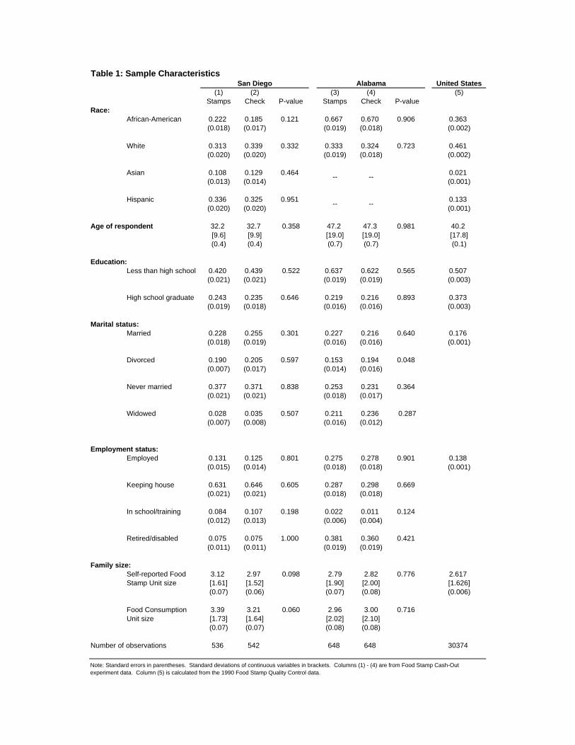
Table 1: Sample CharacteristicsUnited States

(1) (2) (3) (4) (5)Stamps Check P-value Stamps Check P-value

Race:African-American 0.222 0.185 0.121 0.667 0.670 0.906 0.363

(0.018) (0.017) (0.019) (0.018) (0.002)

White 0.313 0.339 0.332 0.333 0.324 0.723 0.461(0.020) (0.020) (0.019) (0.018) (0.002)

Asian 0.108 0.129 0.464 0.021(0.013) (0.014) (0.001)

Hispanic 0.336 0.325 0.951 0.133(0.020) (0.020) (0.001)

Age of respondent 32.2 32.7 0.358 47.2 47.3 0.981 40.2[9.6] [9.9] [19.0] [19.0] [17.8](0.4) (0.4) (0.7) (0.7) (0.1)

Education:Less than high school 0.420 0.439 0.522 0.637 0.622 0.565 0.507

(0.021) (0.021) (0.019) (0.019) (0.003)

High school graduate 0.243 0.235 0.646 0.219 0.216 0.893 0.373(0.019) (0.018) (0.016) (0.016) (0.003)

Marital status:Married 0.228 0.255 0.301 0.227 0.216 0.640 0.176

(0.018) (0.019) (0.016) (0.016) (0.001)

Divorced 0.190 0.205 0.597 0.153 0.194 0.048(0.007) (0.017) (0.014) (0.016)

Never married 0.377 0.371 0.838 0.253 0.231 0.364(0.021) (0.021) (0.018) (0.017)

Widowed 0.028 0.035 0.507 0.211 0.236 0.287(0.007) (0.008) (0.016) (0.012)

Employment status:Employed 0.131 0.125 0.801 0.275 0.278 0.901 0.138

(0.015) (0.014) (0.018) (0.018) (0.001)

Keeping house 0.631 0.646 0.605 0.287 0.298 0.669(0.021) (0.021) (0.018) (0.018)

In school/training 0.084 0.107 0.198 0.022 0.011 0.124(0.012) (0.013) (0.006) (0.004)

Retired/disabled 0.075 0.075 1.000 0.381 0.360 0.421(0.011) (0.011) (0.019) (0.019)

Family size:3.12 2.97 0.098 2.79 2.82 0.776 2.617[1.61] [1.52] [1.90] [2.00] [1.626](0.07) (0.06) (0.07) (0.08) (0.006)

3.39 3.21 0.060 2.96 3.00 0.716[1.73] [1.64] [2.02] [2.10](0.07) (0.07) (0.08) (0.08)

Number of observations 536 542 648 648 30374

Note: Standard errors in parentheses. Standard deviations of continuous variables in brackets. Columns (1) - (4) are from Food Stamp Cash-Out experiment data. Column (5) is calculated from the 1990 Food Stamp Quality Control data.

Self-reported Food Stamp Unit size

Food Consumption Unit size

San Diego Alabama

-- --

-- --

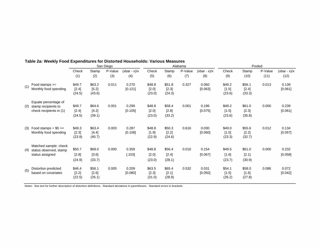
Table 2a: Weekly Food Expenditures for Distorted Households: Various Measures

Check Stamp P-Value (xbar - x)/x Check Stamp P-Value (xbar - x)/x Check Stamp P-Value (xbar - x)/x(1) (2) (3) (4) (5) (6) (7) (8) (9) (10) (11) (12)

$49.7 $63.2 0.011 0.270 $48.8 $51.8 0.327 0.060 $49.2 $56.1 0.013 0.139[2.4] [5.2] [0.121] [2.0] [2.3] [0.063] [1.5] [2.4] [0.061]

(24.5) (43.6) (23.0) (24.3) (23.6) (33.3)

$49.7 $64.6 0.001 0.299 $48.8 $58.4 0.001 0.196 $49.2 $61.0 0.000 0.239[2.4] [4.2] [0.105] [2.0] [2.8] [0.075] [1.5] [2.3] [0.061]

(24.5) (39.1) (23.0) (33.2) (23.6) (35.8)

$49.3 $63.4 0.003 0.287 $48.8 $50.3 0.616 0.030 $49.0 $55.6 0.012 0.134[2.3] [4.4] [0.108] [1.9] [2.2] [0.060] [1.5] [2.2] [0.057]

(23.9) (40.7) (22.9) (24.6) (23.3) (32.7)

$50.7 $69.0 0.000 0.359 $48.8 $56.4 0.016 0.154 $49.5 $61.0 0.000 0.232

[2.8] [3.6] [.103] [2.0] [2.4] [0.067] [1.6] [2.1] [0.058]

(24.9) (33.7) (23.0) (28.1) (23.7) (30.9)

$46.4 $56.1 0.005 0.209 $63.5 $65.4 0.532 0.031 $54.1 $58.0 0.086 0.072[2.2] [2.6] [0.080] [2.3] [2.1] [0.050] [1.5] [1.6] [0.042]

(22.5) (26.1) (31.0) (28.9) (26.2) (27.8)

Distortion predicted based on covariates

(5)

Food stamps >= Monthly food spending

Equate percentage of stamp recipients to check recipients in (1)

Food stamps + $5 >= Monthly food spending

Matched sample: check status observed, stamp status assigned

(1)

(2)

(3)

Pooled

Notes: See text for further description of distortion definitions. Standard deviations in parentheses. Standard errors in brackets.

San Diego Alabama

(4)

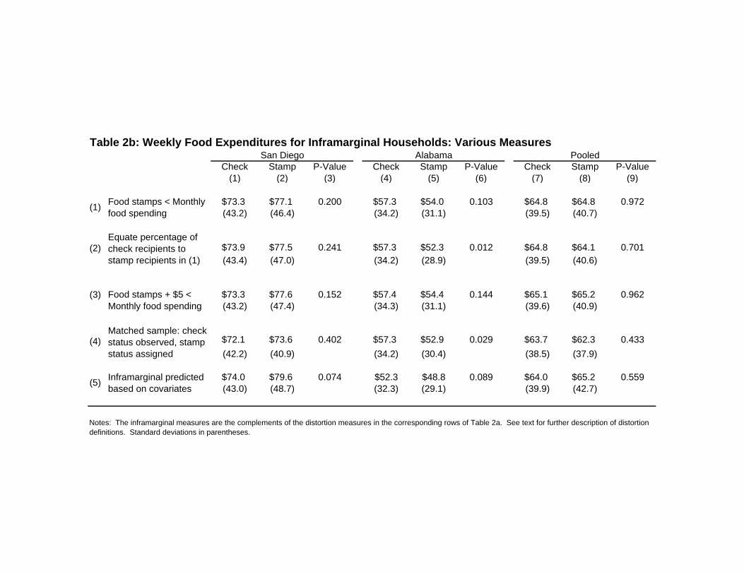
Table 2b: Weekly Food Expenditures for Inframarginal Households: Various Measures

Check Stamp P-Value Check Stamp P-Value Check Stamp P-Value(1) (2) (3) (4) (5) (6) (7) (8) (9)

$73.3 $77.1 0.200 $57.3 $54.0 0.103 $64.8 $64.8 0.972(43.2) (46.4) (34.2) (31.1) (39.5) (40.7)

$73.9 $77.5 0.241 $57.3 $52.3 0.012 $64.8 $64.1 0.701(43.4) (47.0) (34.2) (28.9) (39.5) (40.6)

$73.3 $77.6 0.152 $57.4 $54.4 0.144 $65.1 $65.2 0.962(43.2) (47.4) (34.3) (31.1) (39.6) (40.9)

$72.1 $73.6 0.402 $57.3 $52.9 0.029 $63.7 $62.3 0.433

(42.2) (40.9) (34.2) (30.4) (38.5) (37.9)

$74.0 $79.6 0.074 $52.3 $48.8 0.089 $64.0 $65.2 0.559(43.0) (48.7) (32.3) (29.1) (39.9) (42.7)

(2)

(3)

(4)

San Diego Pooled

Inframarginal predicted based on covariates

Notes: The inframarginal measures are the complements of the distortion measures in the corresponding rows of Table 2a. See text for further description of distortion definitions. Standard deviations in parentheses.

(5)

Food stamps < Monthly food spending

Equate percentage of check recipients to stamp recipients in (1)

Food stamps + $5 < Monthly food spending

Matched sample: check status observed, stamp status assigned

(1)

Alabama

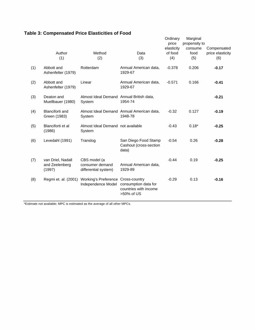
Table 3: Compensated Price Elasticities of Food

Author Method Data

Ordinary price

elasticity of food

Marginal propensity to

consume food

Compensated price elasticity

(1) (2) (3) (4) (5) (6)

(1) Abbott and Ashenfelter (1979)

Rotterdam Annual American data, 1929-67

-0.378 0.206 -0.17

(2) Abbott and Ashenfelter (1979)

Linear Annual American data, 1929-67

-0.571 0.166 -0.41

(3) Deaton and Muellbauer (1980)

Almost Ideal Demand System

Annual British data, 1954-74

-0.21

(4) Blanciforti and Green (1983)

Almost Ideal Demand System

Annual American data, 1948-78

-0.32 0.127 -0.19

(5) Blanciforti et al (1986)

Almost Ideal Demand System

not available -0.43 0.18* -0.25

(6) Levedahl (1991) Translog San Diego Food Stamp Cashout (cross-section data)

-0.54 0.26 -0.28

(7) van Driel, Nadall and Zeelenberg (1997)

CBS model (a consumer demand differential system)

Annual American data, 1929-89

-0.44 0.19 -0.25

(8) Regmi et. al. (2001) Working's Preference Independence Model

Cross-country consumption data for countries with income >50% of US

-0.29 0.13 -0.16

*Estimate not available; MPC is estimated as the average of all other MPCs.

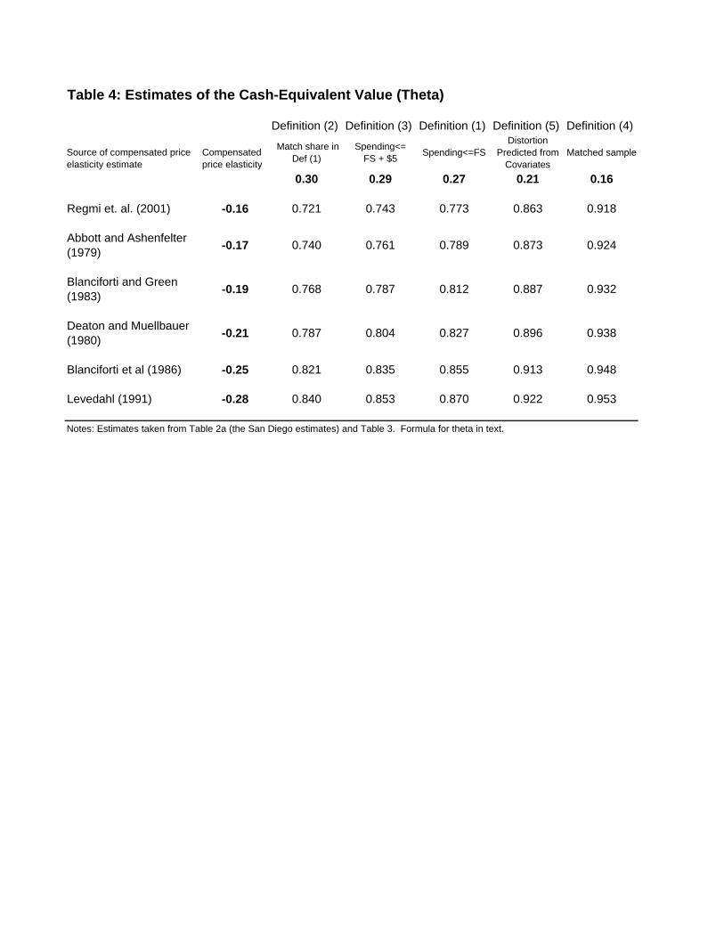
Table 4: Estimates of the Cash-Equivalent Value (Theta)

Definition (2) Definition (3) Definition (1) Definition (5) Definition (4)

Source of compensated price elasticity estimate

Compensated price elasticity

Match share in Def (1)

Spending<= FS + $5

Spending<=FSDistortion

Predicted from Covariates

Matched sample

0.30 0.29 0.27 0.21 0.16

Regmi et. al. (2001) -0.16 0.721 0.743 0.773 0.863 0.918

Abbott and Ashenfelter (1979)

-0.17 0.740 0.761 0.789 0.873 0.924

Blanciforti and Green (1983)

-0.19 0.768 0.787 0.812 0.887 0.932

Deaton and Muellbauer (1980)

-0.21 0.787 0.804 0.827 0.896 0.938

Blanciforti et al (1986) -0.25 0.821 0.835 0.855 0.913 0.948

Levedahl (1991) -0.28 0.840 0.853 0.870 0.922 0.953

Notes: Estimates taken from Table 2a (the San Diego estimates) and Table 3. Formula for theta in text.

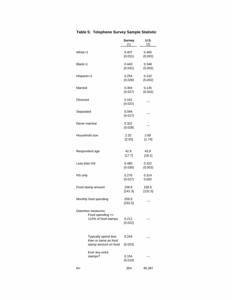
Table 5: Telephone Survey Sample Statistics

Survey U.S.(1) (2)

White=1 0.407 0.465(0.031) (0.002)

Black=1 0.443 0.348(0.031) (0.002)

Hispanic=1 0.254 0.142(0.026) (0.002)

Married 0.304 0.135(0.027) (0.002)

Divorced 0.161(0.022)

Separated 0.094(0.017)

Never married 0.322(0.028)

Household size 2.32 2.60[2.02] [1.74]

Respondent age 42.9 43.9[17.7] [18.1]

Less than HS 0.480 0.322(0.030) (0.002)

HS only 0.276 0.314(0.027) 0.002

Food stamp amount 158.9 156.6[141.3] [131.5]

Monthly food spending 259.9[152.5]

Distortion measures:Food spending <= 110% of food stamps 0.212

(0.022)

0.244

(0.023)

Ever any extra stamps? 0.154

(0.019)

N= 354 45,387

---

Typically spend less than or same as food stamp amount on food

---

---

---

---

---

---

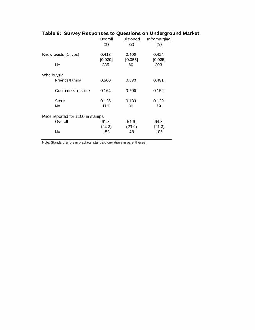
Table 6: Survey Responses to Questions on Underground MarketOverall Distorted Inframarginal

(1) (2) (3)

Know exists (1=yes) 0.418 0.400 0.424[0.029] [0.055] [0.035]

N= 285 80 203

Who buys?Friends/family 0.500 0.533 0.481

Customers in store 0.164 0.200 0.152

Store 0.136 0.133 0.139N= 110 30 79

Price reported for $100 in stampsOverall 61.3 54.6 64.3

(24.3) (29.0) (21.3)N= 153 48 105

Note: Standard errors in brackets; standard deviations in parentheses.

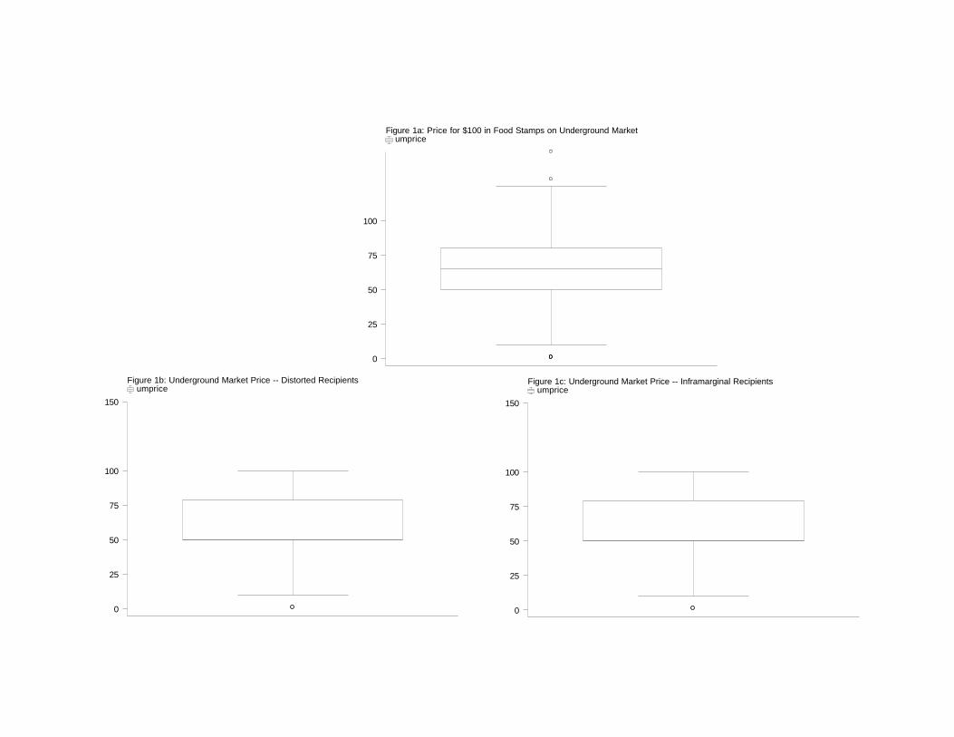
Figure 1a: Price for $100 in Food Stamps on Underground Market

0

25

50

75

100

umprice

Figure 1b: Underground Market Price -- Distorted Recipients

0

25

50

75

100

150

umpriceFigure 1c: Underground Market Price -- Inframarginal Recipients

0

25

50

75

100

150

umprice

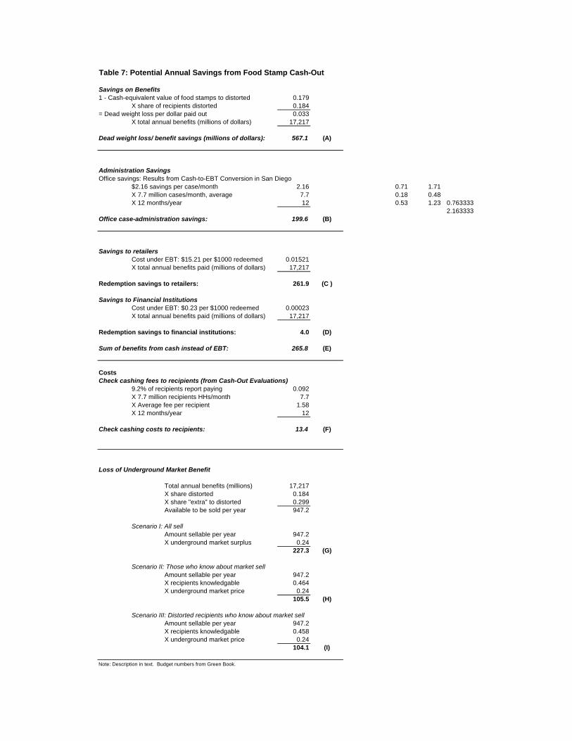
Table 7: Potential Annual Savings from Food Stamp Cash-Out

Savings on Benefits1 - Cash-equivalent value of food stamps to distorted 0.179

X share of recipients distorted 0.184= Dead weight loss per dollar paid out 0.033

X total annual benefits (millions of dollars) 17,217

Dead weight loss/ benefit savings (millions of dollars): 567.1 (A)

Administration SavingsOffice savings: Results from Cash-to-EBT Conversion in San Diego

$2.16 savings per case/month 2.16 0.71 1.71X 7.7 million cases/month, average 7.7 0.18 0.48X 12 months/year 12 0.53 1.23 0.763333

2.163333Office case-administration savings: 199.6 (B)

Savings to retailersCost under EBT: $15.21 per $1000 redeemed 0.01521X total annual benefits paid (millions of dollars) 17,217

Redemption savings to retailers: 261.9 (C )

Savings to Financial InstitutionsCost under EBT: $0.23 per $1000 redeemed 0.00023X total annual benefits paid (millions of dollars) 17,217

Redemption savings to financial institutions: 4.0 (D)

Sum of benefits from cash instead of EBT: 265.8 (E)

CostsCheck cashing fees to recipients (from Cash-Out Evaluations)

9.2% of recipients report paying 0.092X 7.7 million recipients HHs/month 7.7X Average fee per recipient 1.58X 12 months/year 12

Check cashing costs to recipients: 13.4 (F)

Loss of Underground Market Benefit

Total annual benefits (millions) 17,217X share distorted 0.184X share "extra" to distorted 0.299Available to be sold per year 947.2

Scenario I: All sellAmount sellable per year 947.2X underground market surplus 0.24

227.3 (G)

Scenario II: Those who know about market sellAmount sellable per year 947.2X recipients knowledgable 0.464X underground market price 0.24

105.5 (H)

Scenario III: Distorted recipients who know about market sellAmount sellable per year 947.2X recipients knowledgable 0.458X underground market price 0.24

104.1 (I)

Note: Description in text. Budget numbers from Green Book.

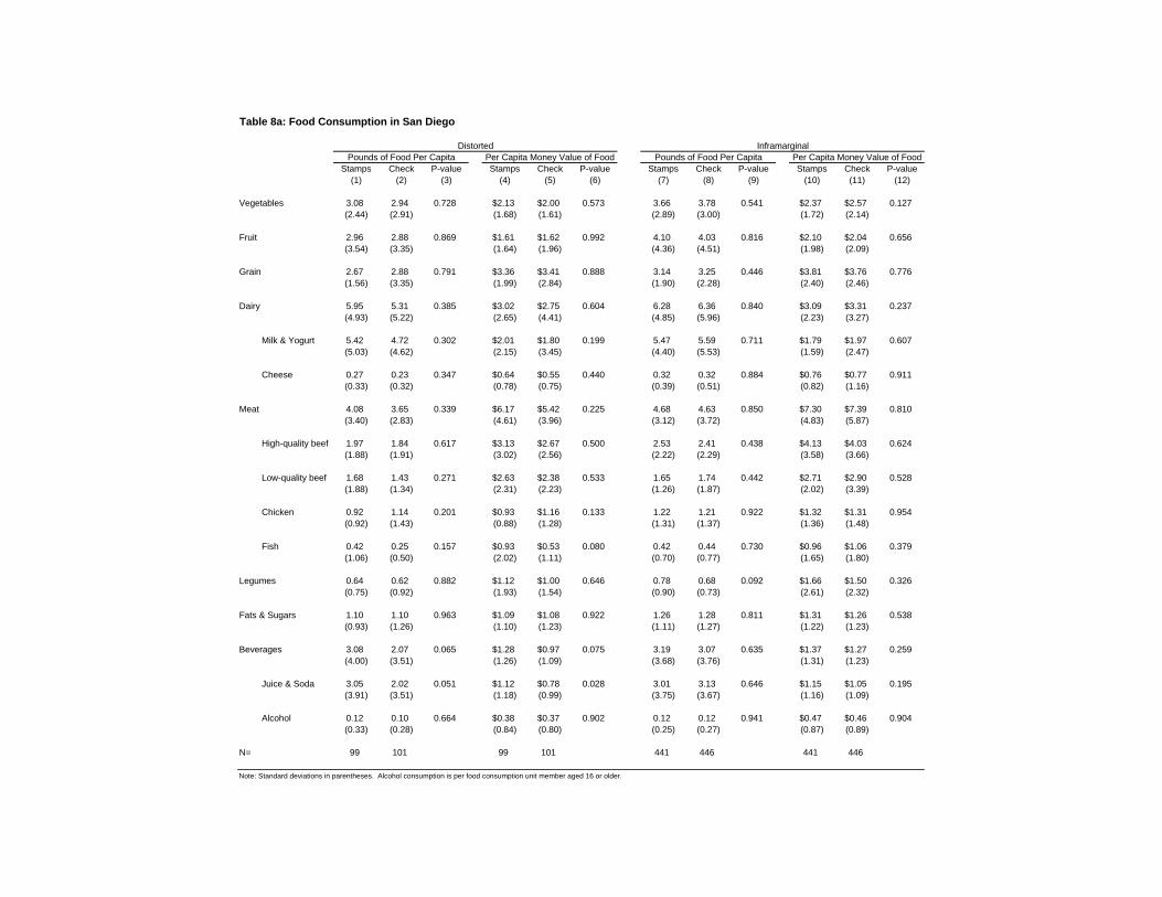
Table 8a: Food Consumption in San Diego

Stamps Check P-value Stamps Check P-value Stamps Check P-value Stamps Check P-value(1) (2) (3) (4) (5) (6) (7) (8) (9) (10) (11) (12)

Vegetables 3.08 2.94 0.728 $2.13 $2.00 0.573 3.66 3.78 0.541 $2.37 $2.57 0.127(2.44) (2.91) (1.68) (1.61) (2.89) (3.00) (1.72) (2.14)

Fruit 2.96 2.88 0.869 $1.61 $1.62 0.992 4.10 4.03 0.816 $2.10 $2.04 0.656(3.54) (3.35) (1.64) (1.96) (4.36) (4.51) (1.98) (2.09)

Grain 2.67 2.88 0.791 $3.36 $3.41 0.888 3.14 3.25 0.446 $3.81 $3.76 0.776(1.56) (3.35) (1.99) (2.84) (1.90) (2.28) (2.40) (2.46)

Dairy 5.95 5.31 0.385 $3.02 $2.75 0.604 6.28 6.36 0.840 $3.09 $3.31 0.237(4.93) (5.22) (2.65) (4.41) (4.85) (5.96) (2.23) (3.27)

Milk & Yogurt 5.42 4.72 0.302 $2.01 $1.80 0.199 5.47 5.59 0.711 $1.79 $1.97 0.607(5.03) (4.62) (2.15) (3.45) (4.40) (5.53) (1.59) (2.47)

Cheese 0.27 0.23 0.347 $0.64 $0.55 0.440 0.32 0.32 0.884 $0.76 $0.77 0.911(0.33) (0.32) (0.78) (0.75) (0.39) (0.51) (0.82) (1.16)

Meat 4.08 3.65 0.339 $6.17 $5.42 0.225 4.68 4.63 0.850 $7.30 $7.39 0.810(3.40) (2.83) (4.61) (3.96) (3.12) (3.72) (4.83) (5.87)

High-quality beef 1.97 1.84 0.617 $3.13 $2.67 0.500 2.53 2.41 0.438 $4.13 $4.03 0.624(1.88) (1.91) (3.02) (2.56) (2.22) (2.29) (3.58) (3.66)

Low-quality beef 1.68 1.43 0.271 $2.63 $2.38 0.533 1.65 1.74 0.442 $2.71 $2.90 0.528(1.88) (1.34) (2.31) (2.23) (1.26) (1.87) (2.02) (3.39)

Chicken 0.92 1.14 0.201 $0.93 $1.16 0.133 1.22 1.21 0.922 $1.32 $1.31 0.954(0.92) (1.43) (0.88) (1.28) (1.31) (1.37) (1.36) (1.48)

Fish 0.42 0.25 0.157 $0.93 $0.53 0.080 0.42 0.44 0.730 $0.96 $1.06 0.379(1.06) (0.50) (2.02) (1.11) (0.70) (0.77) (1.65) (1.80)

Legumes 0.64 0.62 0.882 $1.12 $1.00 0.646 0.78 0.68 0.092 $1.66 $1.50 0.326(0.75) (0.92) (1.93) (1.54) (0.90) (0.73) (2.61) (2.32)

Fats & Sugars 1.10 1.10 0.963 $1.09 $1.08 0.922 1.26 1.28 0.811 $1.31 $1.26 0.538(0.93) (1.26) (1.10) (1.23) (1.11) (1.27) (1.22) (1.23)

Beverages 3.08 2.07 0.065 $1.28 $0.97 0.075 3.19 3.07 0.635 $1.37 $1.27 0.259(4.00) (3.51) (1.26) (1.09) (3.68) (3.76) (1.31) (1.23)

Juice & Soda 3.05 2.02 0.051 $1.12 $0.78 0.028 3.01 3.13 0.646 $1.15 $1.05 0.195(3.91) (3.51) (1.18) (0.99) (3.75) (3.67) (1.16) (1.09)

Alcohol 0.12 0.10 0.664 $0.38 $0.37 0.902 0.12 0.12 0.941 $0.47 $0.46 0.904(0.33) (0.28) (0.84) (0.80) (0.25) (0.27) (0.87) (0.89)

N= 99 101 99 101 441 446 441 446

Note: Standard deviations in parentheses. Alcohol consumption is per food consumption unit member aged 16 or older.

InframarginalDistortedPounds of Food Per Capita Per Capita Money Value of Food Pounds of Food Per Capita Per Capita Money Value of Food

Table 8b: Food Consumption in Alabama

Stamps Check P-value Stamps Check P-value Stamps Check P-value Stamps Check P-value(1) (2) (3) (4) (5) (6) (7) (8) (9) (10) (11) (12)

Vegetables 2.61 2.17 0.041 $1.62 $1.44 0.216 4.75 4.78 0.905 $3.01 $3.15 0.331(1.84) (1.65) (0.93) (1.38) (3.38) (4.06) (2.08) (2.62)

Fruit 2.05 1.67 0.274 $0.81 $0.62 0.080 3.76 3.84 0.833 $1.62 $1.72 0.388(3.13) (2.63) (1.05) (0.69) (5.81) (5.78) (1.74) (2.00)

Grain 1.91 2.04 0.246 $1.80 $1.95 0.223 3.35 3.51 0.221 $3.16 $3.36 0.109(0.93) (1.03) (1.01) (1.01) (2.12) (2.07) (1.92) (2.04)

Dairy 2.59 2.81 0.394 $1.39 $1.48 0.585 4.56 5.17 0.024 $2.39 $2.69 0.022(2.00) (2.22) (1.23) (1.27) (3.67) (4.88) (1.85) (2.32)

Milk & Yogurt 2.31 2.50 0.439 $0.90 $1.00 0.394 3.98 4.48 0.053 $1.45 $1.65 0.03815 (1.85) (2.17) (0.87) (1.08) (3.51) (4.64) (1.33) (1.66)

Cheese 0.13 0.13 0.914 $0.33 $0.31 0.728 0.19 0.24 0.006 $0.49 $0.59 0.02316 (0.21) (0.15) (0.57) (0.39) (0.27) (0.33) (0.66) (0.77)

Meat 3.96 4.18 0.382 $5.24 $5.29 0.859 6.60 6.65 0.854 $9.19 $9.28 0.812(2.20) (1.87) (2.71) (2.20) (4.30) (4.29) (5.66) (5.81)

High-quality beef 1.89 2.06 0.309 $2.31 $2.59 0.151 2.96 3.23 0.111 $4.17 $4.57 0.092(1.34) (1.45) (1.50) (1.70) (2.58) (2.82) (3.61) (3.97)

Low-quality beef 1.72 1.70 0.872 $2.69 $2.42 0.176 2.99 2.79 0.155 $4.60 $4.29 0.125(1.21) (0.97) (1.84) (1.43) (2.34) (2.21) (3.12) (3.21)

Chicken 1.17 1.09 0.520 $1.06 $1.01 0.601 1.53 1.70 0.115 $1.49 $1.64 0.12520 (1.04) (0.94) (0.82) (0.85) (1.50) (1.90) (1.43) (1.74)

Fish 0.23 0.34 0.050 $0.42 $0.47 0.597 0.56 0.62 0.352 $0.90 $1.06 0.16721 (0.33) (0.57) (0.72) (0.71) (0.94) (1.15) (1.43) (2.17)

Legumes 0.48 0.54 0.356 $0.76 $0.59 0.154 0.89 0.80 0.151 $1.21 $1.13 0.400(0.50) (0.68) (1.15) (0.78) (1.05) (0.83) (1.71) (1.54)

Fats & Sugars 1.07 1.10 0.766 $0.69 $0.71 0.785 1.76 1.90 0.135 $1.40 $1.44 0.574(0.80) (0.91) (0.50) (0.61) (1.41) (1.56) (1.21) (1.26)

Beverages 2.44 2.11 0.259 $0.93 $0.87 0.582 4.14 3.63 0.057 $1.76 $1.65 0.271(2.46) (2.42) (0.79) (0.86) (4.52) (4.10) (1.61) (1.44)

Juice & Soda 2.40 2.06 0.239 $0.82 $0.70 0.213 4.01 3.50 0.062 $1.28 $1.15 0.12030 (2.45) (2.41) (0.75) (0.77) (4.52) (4.08) (1.43) (1.21)

Alcohol 0.03 0.07 0.343 $0.04 $0.06 0.597 0.11 0.09 0.718 $0.08 $0.07 0.85532 (0.18) (0.36) (0.21) (0.34) (0.69) (0.65) (0.66) (0.47)

0.00N= 138 138 138 138 510 510 510 510

Note: Standard deviations in parentheses. Alcohol consumption is per food consumption unit member aged 16 or older.

InframarginalDistortedPounds of Food Per Capita Per Capita Money Value of Food Pounds of Food Per Capita Per Capita Money Value of Food

Table 8c: Food Consumption -- Pooled Sites

Stamps Check P-value Stamps Check P-value Stamps Check P-value Stamps Check P-value(1) (2) (3) (4) (5) (6) (7) (8) (9) (10) (11) (12)

Vegetables 2.85 2.50 0.085 $1.85 $1.68 0.193 4.24 4.31 0.637 $2.71 $2.88 0.094(2.11) (2.30) (1.30) (1.51) (3.21) (3.64) (1.95) (2.43)

Fruit 2.49 2.18 0.300 $1.16 $1.04 0.351 3.91 3.93 0.955 $1.84 $1.87 0.755(3.37) (3.01) (1.41) (1.46) (5.19) (5.22) (1.87) (2.05)

Grain 2.21 2.28 0.604 $2.43 $2.57 0.434 3.26 3.39 0.185 $3.47 $3.54 0.447(1.26) (1.55) (1.65) (2.12) (2.03) (2.17) (2.18) (2.25)

Dairy 4.04 3.87 0.633 $2.09 $2.01 0.745 5.35 5.72 0.094 $2.71 $2.98 0.017(4.16) (3.97) (2.12) (3.08) (4.28) (5.44) (2.05) (2.82)

Milk & Yogurt 3.61 3.43 0.609 $1.36 $1.34 0.894 4.67 5.00 0.118 $1.61 $1.80 0.02215 (3.85) (3.59) (1.63) (2.42) (4.02) (5.10) (1.47) (2.08)

Cheese 0.19 0.17 0.424 $0.46 $0.41 0.432 0.25 0.28 0.140 $0.61 $0.67 0.14016 (0.28) (0.24) (0.68) (0.58) (0.34) (0.43) (0.75) (0.97)

Meat 4.02 3.96 0.774 $5.65 $5.35 0.328 5.71 5.71 0.992 $8.32 $8.40 0.772(2.71) (2.33) (3.58) (3.06) (3.92) (4.16) (5.38) (5.91)

High-quality beef 1.92 1.96 0.774 $2.66 $2.63 0.882 2.76 2.85 0.447 $4.15 $4.32 0.333(1.58) (1.66) (2.89) (2.10) (2.43) (2.62) (3.60) (3.84)

Low-quality beef 1.71 1.58 0.320 $2.67 $2.41 0.142 2.37 2.30 0.440 $3.72 $3.64 0.574(1.52) (1.14) (2.05) (1.81) (2.03) (2.12) (2.83) (3.37)

Chicken 1.06 1.11 0.640 $1.00 $1.07 0.436 1.39 1.47 0.233 $1.41 $1.49 0.25920 (1.00) (1.17) (0.85) (1.05) (1.42) (1.69) (1.40) (1.63)

Fish 0.31 0.30 0.932 $0.64 $0.49 0.195 0.49 0.53 0.340 $0.93 $1.06 0.10521 (0.73) (0.54) (1.44) (0.90) (0.84) (1.00) (1.54) (2.00)

Legumes 0.54 0.58 0.614 $0.91 $0.76 0.240 0.84 0.75 0.027 $1.43 $1.30 0.190(0.61) (0.79) (1.50) (1.18) (0.98) (0.78) (2.19) (1.95)

Fats & Sugars 1.08 1.10 0.795 $0.86 $0.87 0.912 1.53 1.61 0.209 $1.36 $1.36 0.954(0.84) (1.07) (0.81) (0.94) (1.31) (1.46) (1.22) (1.25)

Beverages 2.72 2.09 0.026 $1.08 $0.92 0.075 3.70 3.37 0.076 $1.58 $1.48 0.121(3.17) (2.93) (1.04) (0.96) (4.18) (3.95) (1.49) (1.36)

Juice & Soda 2.67 2.04 0.024 $0.94 $0.74 0.014 3.60 3.27 0.080 $1.22 $1.11 0.04330 (3.15) (2.92) (0.96) (0.87) (4.17) (3.94) (1.32) (1.16)

Alcohol 0.11 0.07 0.546 $0.09 $0.07 0.694 0.17 0.14 0.400 $0.13 $0.15 0.66632 (0.79) (0.36) (0.52) (0.36) (1.00) (0.78) (0.76) (0.89)

N= 237 239 237 239 951 956 951 956

Note: Standard deviations in parentheses. Alcohol consumption is per food consumption unit member aged 16 or older.

InframarginalDistortedPounds of Food Per Capita Per Capita Money Value of Food Pounds of Food Per Capita Per Capita Money Value of Food

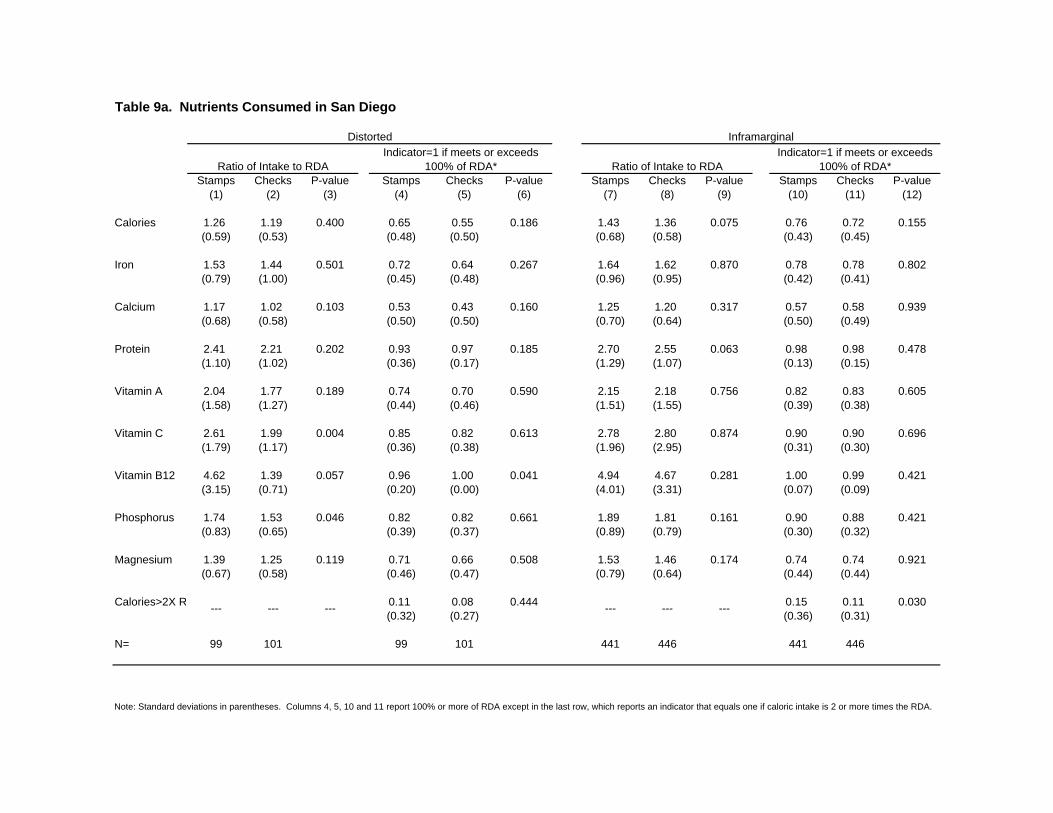
Table 9a. Nutrients Consumed in San Diego

Stamps Checks P-value Stamps Checks P-value Stamps Checks P-value Stamps Checks P-value(1) (2) (3) (4) (5) (6) (7) (8) (9) (10) (11) (12)

Calories 1.26 1.19 0.400 0.65 0.55 0.186 1.43 1.36 0.075 0.76 0.72 0.155(0.59) (0.53) (0.48) (0.50) (0.68) (0.58) (0.43) (0.45)

Iron 1.53 1.44 0.501 0.72 0.64 0.267 1.64 1.62 0.870 0.78 0.78 0.802(0.79) (1.00) (0.45) (0.48) (0.96) (0.95) (0.42) (0.41)

Calcium 1.17 1.02 0.103 0.53 0.43 0.160 1.25 1.20 0.317 0.57 0.58 0.939(0.68) (0.58) (0.50) (0.50) (0.70) (0.64) (0.50) (0.49)

Protein 2.41 2.21 0.202 0.93 0.97 0.185 2.70 2.55 0.063 0.98 0.98 0.478(1.10) (1.02) (0.36) (0.17) (1.29) (1.07) (0.13) (0.15)

Vitamin A 2.04 1.77 0.189 0.74 0.70 0.590 2.15 2.18 0.756 0.82 0.83 0.605(1.58) (1.27) (0.44) (0.46) (1.51) (1.55) (0.39) (0.38)

Vitamin C 2.61 1.99 0.004 0.85 0.82 0.613 2.78 2.80 0.874 0.90 0.90 0.696(1.79) (1.17) (0.36) (0.38) (1.96) (2.95) (0.31) (0.30)

Vitamin B12 4.62 1.39 0.057 0.96 1.00 0.041 4.94 4.67 0.281 1.00 0.99 0.421(3.15) (0.71) (0.20) (0.00) (4.01) (3.31) (0.07) (0.09)

Phosphorus 1.74 1.53 0.046 0.82 0.82 0.661 1.89 1.81 0.161 0.90 0.88 0.421(0.83) (0.65) (0.39) (0.37) (0.89) (0.79) (0.30) (0.32)

Magnesium 1.39 1.25 0.119 0.71 0.66 0.508 1.53 1.46 0.174 0.74 0.74 0.921(0.67) (0.58) (0.46) (0.47) (0.79) (0.64) (0.44) (0.44)

Calories>2X RDA 0.11 0.08 0.444 0.15 0.11 0.030(0.32) (0.27) (0.36) (0.31)

N= 99 101 99 101 441 446 441 446

Ratio of Intake to RDAIndicator=1 if meets or exceeds

100% of RDA*

Note: Standard deviations in parentheses. Columns 4, 5, 10 and 11 report 100% or more of RDA except in the last row, which reports an indicator that equals one if caloric intake is 2 or more times the RDA.

Distorted Inframarginal

--- --- --- --- --- ---

Ratio of Intake to RDAIndicator=1 if meets or exceeds

100% of RDA*

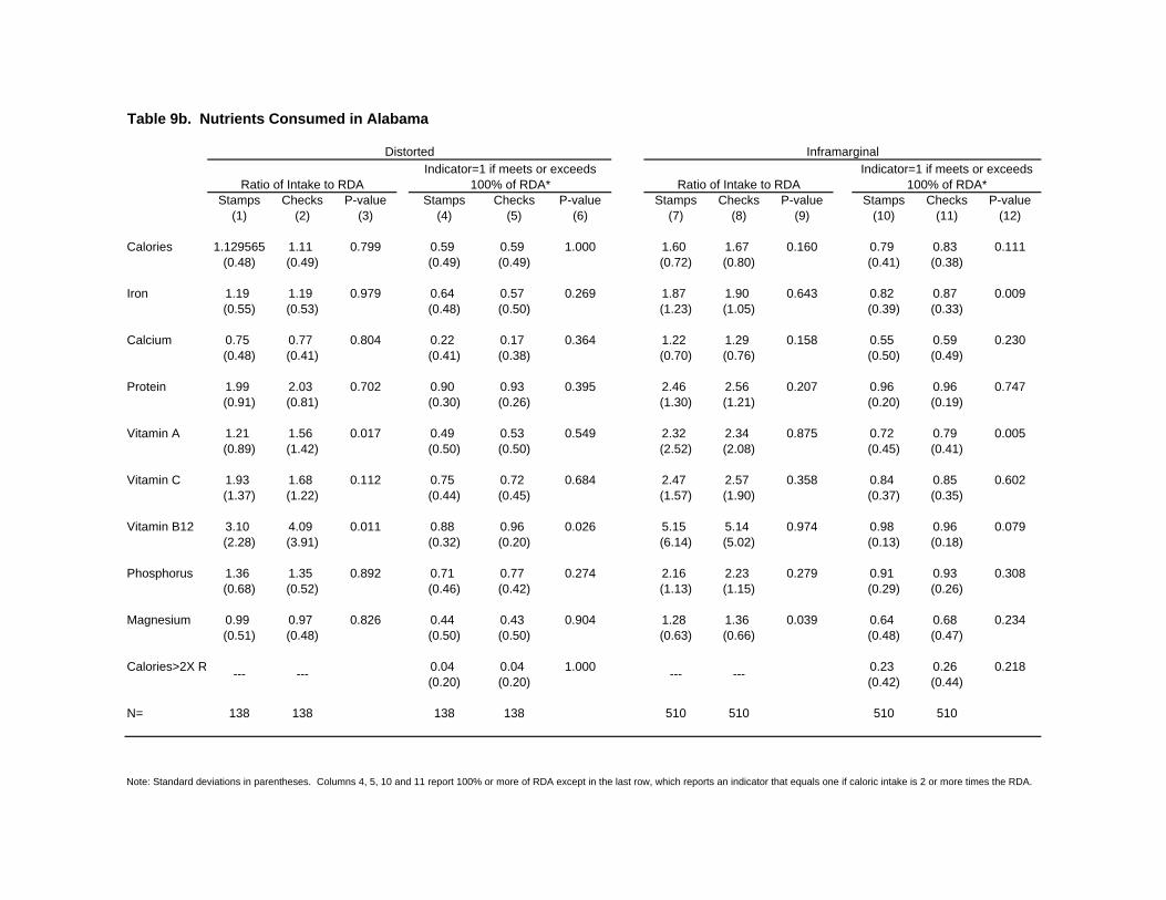
Table 9b. Nutrients Consumed in Alabama

Stamps Checks P-value Stamps Checks P-value Stamps Checks P-value Stamps Checks P-value(1) (2) (3) (4) (5) (6) (7) (8) (9) (10) (11) (12)

Calories 1.129565 1.11 0.799 0.59 0.59 1.000 1.60 1.67 0.160 0.79 0.83 0.111(0.48) (0.49) (0.49) (0.49) (0.72) (0.80) (0.41) (0.38)

Iron 1.19 1.19 0.979 0.64 0.57 0.269 1.87 1.90 0.643 0.82 0.87 0.009(0.55) (0.53) (0.48) (0.50) (1.23) (1.05) (0.39) (0.33)

Calcium 0.75 0.77 0.804 0.22 0.17 0.364 1.22 1.29 0.158 0.55 0.59 0.230(0.48) (0.41) (0.41) (0.38) (0.70) (0.76) (0.50) (0.49)

Protein 1.99 2.03 0.702 0.90 0.93 0.395 2.46 2.56 0.207 0.96 0.96 0.747(0.91) (0.81) (0.30) (0.26) (1.30) (1.21) (0.20) (0.19)

Vitamin A 1.21 1.56 0.017 0.49 0.53 0.549 2.32 2.34 0.875 0.72 0.79 0.005(0.89) (1.42) (0.50) (0.50) (2.52) (2.08) (0.45) (0.41)

Vitamin C 1.93 1.68 0.112 0.75 0.72 0.684 2.47 2.57 0.358 0.84 0.85 0.602(1.37) (1.22) (0.44) (0.45) (1.57) (1.90) (0.37) (0.35)

Vitamin B12 3.10 4.09 0.011 0.88 0.96 0.026 5.15 5.14 0.974 0.98 0.96 0.079(2.28) (3.91) (0.32) (0.20) (6.14) (5.02) (0.13) (0.18)

Phosphorus 1.36 1.35 0.892 0.71 0.77 0.274 2.16 2.23 0.279 0.91 0.93 0.308(0.68) (0.52) (0.46) (0.42) (1.13) (1.15) (0.29) (0.26)

Magnesium 0.99 0.97 0.826 0.44 0.43 0.904 1.28 1.36 0.039 0.64 0.68 0.234(0.51) (0.48) (0.50) (0.50) (0.63) (0.66) (0.48) (0.47)

Calories>2X RDA 0.04 0.04 1.000 0.23 0.26 0.218(0.20) (0.20) (0.42) (0.44)

N= 138 138 138 138 510 510 510 510

Ratio of Intake to RDAIndicator=1 if meets or exceeds

100% of RDA* Ratio of Intake to RDAIndicator=1 if meets or exceeds

100% of RDA*

Note: Standard deviations in parentheses. Columns 4, 5, 10 and 11 report 100% or more of RDA except in the last row, which reports an indicator that equals one if caloric intake is 2 or more times the RDA.

Distorted Inframarginal

--- --- --- ---

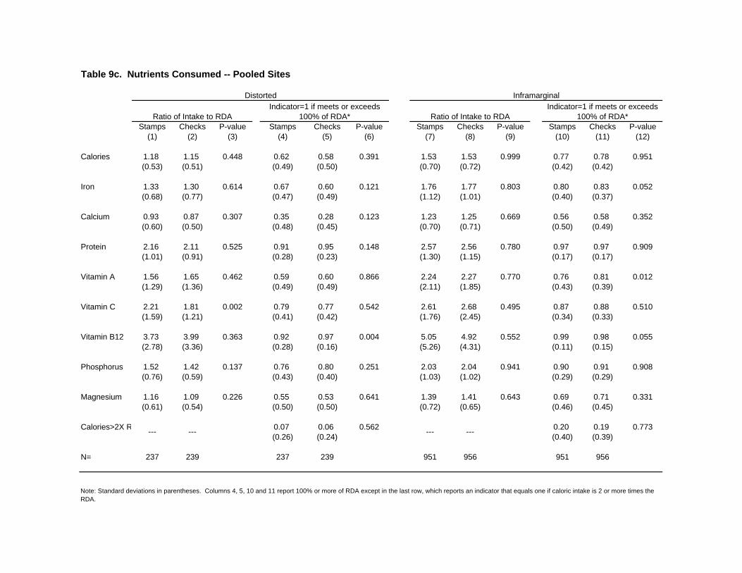
Table 9c. Nutrients Consumed -- Pooled Sites

Stamps Checks P-value Stamps Checks P-value Stamps Checks P-value Stamps Checks P-value(1) (2) (3) (4) (5) (6) (7) (8) (9) (10) (11) (12)

Calories 1.18 1.15 0.448 0.62 0.58 0.391 1.53 1.53 0.999 0.77 0.78 0.951(0.53) (0.51) (0.49) (0.50) (0.70) (0.72) (0.42) (0.42)

Iron 1.33 1.30 0.614 0.67 0.60 0.121 1.76 1.77 0.803 0.80 0.83 0.052(0.68) (0.77) (0.47) (0.49) (1.12) (1.01) (0.40) (0.37)

Calcium 0.93 0.87 0.307 0.35 0.28 0.123 1.23 1.25 0.669 0.56 0.58 0.352(0.60) (0.50) (0.48) (0.45) (0.70) (0.71) (0.50) (0.49)

Protein 2.16 2.11 0.525 0.91 0.95 0.148 2.57 2.56 0.780 0.97 0.97 0.909(1.01) (0.91) (0.28) (0.23) (1.30) (1.15) (0.17) (0.17)

Vitamin A 1.56 1.65 0.462 0.59 0.60 0.866 2.24 2.27 0.770 0.76 0.81 0.012(1.29) (1.36) (0.49) (0.49) (2.11) (1.85) (0.43) (0.39)

Vitamin C 2.21 1.81 0.002 0.79 0.77 0.542 2.61 2.68 0.495 0.87 0.88 0.510(1.59) (1.21) (0.41) (0.42) (1.76) (2.45) (0.34) (0.33)

Vitamin B12 3.73 3.99 0.363 0.92 0.97 0.004 5.05 4.92 0.552 0.99 0.98 0.055(2.78) (3.36) (0.28) (0.16) (5.26) (4.31) (0.11) (0.15)

Phosphorus 1.52 1.42 0.137 0.76 0.80 0.251 2.03 2.04 0.941 0.90 0.91 0.908(0.76) (0.59) (0.43) (0.40) (1.03) (1.02) (0.29) (0.29)

Magnesium 1.16 1.09 0.226 0.55 0.53 0.641 1.39 1.41 0.643 0.69 0.71 0.331(0.61) (0.54) (0.50) (0.50) (0.72) (0.65) (0.46) (0.45)

Calories>2X RDA 0.07 0.06 0.562 0.20 0.19 0.773(0.26) (0.24) (0.40) (0.39)

N= 237 239 237 239 951 956 951 956

Indicator=1 if meets or exceeds 100% of RDA*

Note: Standard deviations in parentheses. Columns 4, 5, 10 and 11 report 100% or more of RDA except in the last row, which reports an indicator that equals one if caloric intake is 2 or more times the RDA.

Distorted Inframarginal

--- --- --- ---

Ratio of Intake to RDAIndicator=1 if meets or exceeds

100% of RDA* Ratio of Intake to RDA

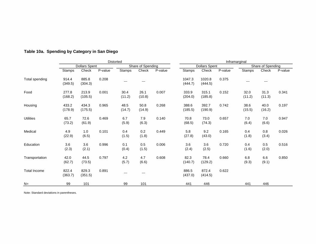
Table 10a. Spending by Category in San Diego

Stamps Check P-value Stamps Check P-value Stamps Check P-value Stamps Check P-value

Total spending 914.4 885.8 0.208 1047.3 1020.8 0.375(349.5) (304.3) (444.7) (444.5)

Food 277.8 213.9 0.001 30.4 26.1 0.007 333.9 315.1 0.152 32.0 31.3 0.341(168.2) (105.5) (11.2) (10.8) (204.0) (185.8) (11.2) (11.3)

Housing 433.2 434.3 0.965 48.5 50.8 0.268 388.6 392.7 0.742 38.6 40.0 0.197(178.9) (175.5) (14.7) (14.9) (185.5) (190.9) (15.5) (16.2)

Utilities 65.7 72.6 0.469 6.7 7.9 0.140 70.8 73.0 0.657 7.0 7.0 0.947(73.2) (61.9) (5.9) (6.3) (68.5) (74.3) (6.4) (6.6)

Medical 4.9 1.0 0.101 0.4 0.2 0.449 5.8 9.2 0.165 0.4 0.8 0.026(22.9) (6.5) (1.5) (1.8) (27.8) (43.0) (1.8) (3.4)

Education 3.6 3.6 0.996 0.1 0.5 0.006 3.6 3.6 0.720 0.4 0.5 0.516(2.3) (2.1) (0.4) (1.5) (2.4) (2.5) (1.6) (2.0)

Transportation 42.0 44.5 0.797 4.2 4.7 0.608 82.3 78.4 0.660 6.8 6.6 0.850(62.7) (73.5) (5.7) (6.6) (140.7) (129.2) (9.3) (9.1)

Total Income 822.4 829.3 0.891 886.5 872.4 0.622(363.7) (351.5) (437.0) (414.5)

N= 99 101 99 101 441 446 441 446

Note: Standard deviations in parentheses.

InframarginalDollars Spent Share of Spending

--- ---

--- ---

Distorted

--- ---

Dollars Spent Share of Spending

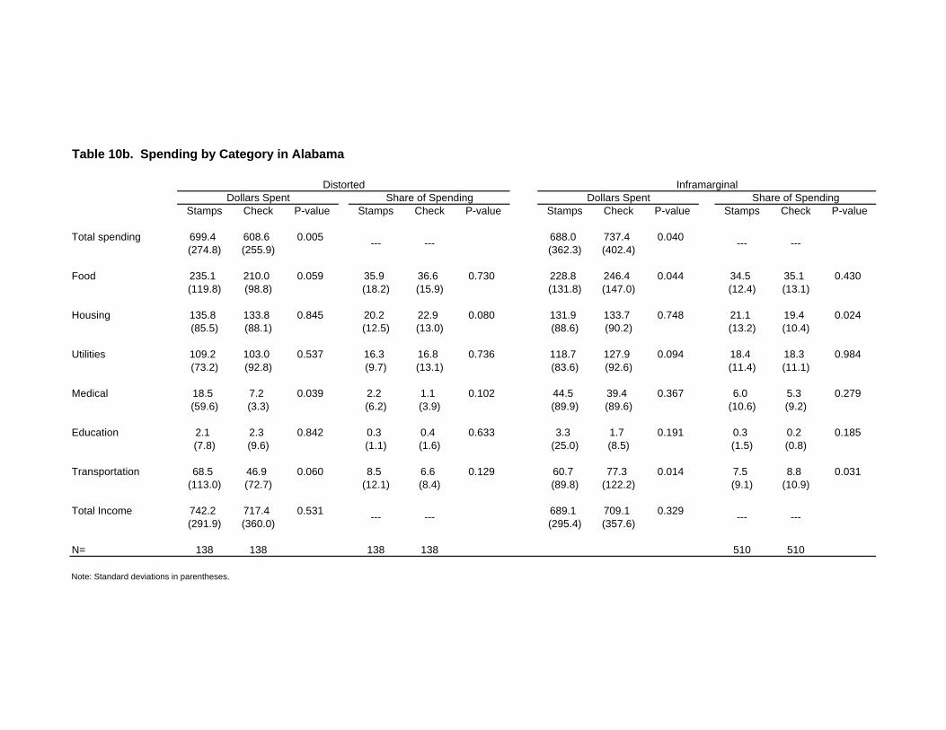
Table 10b. Spending by Category in Alabama

Stamps Check P-value Stamps Check P-value Stamps Check P-value Stamps Check P-value

Total spending 699.4 608.6 0.005 688.0 737.4 0.040(274.8) (255.9) (362.3) (402.4)

Food 235.1 210.0 0.059 35.9 36.6 0.730 228.8 246.4 0.044 34.5 35.1 0.430(119.8) (98.8) (18.2) (15.9) (131.8) (147.0) (12.4) (13.1)

Housing 135.8 133.8 0.845 20.2 22.9 0.080 131.9 133.7 0.748 21.1 19.4 0.024(85.5) (88.1) (12.5) (13.0) (88.6) (90.2) (13.2) (10.4)

Utilities 109.2 103.0 0.537 16.3 16.8 0.736 118.7 127.9 0.094 18.4 18.3 0.984(73.2) (92.8) (9.7) (13.1) (83.6) (92.6) (11.4) (11.1)

Medical 18.5 7.2 0.039 2.2 1.1 0.102 44.5 39.4 0.367 6.0 5.3 0.279(59.6) (3.3) (6.2) (3.9) (89.9) (89.6) (10.6) (9.2)

Education 2.1 2.3 0.842 0.3 0.4 0.633 3.3 1.7 0.191 0.3 0.2 0.185(7.8) (9.6) (1.1) (1.6) (25.0) (8.5) (1.5) (0.8)

Transportation 68.5 46.9 0.060 8.5 6.6 0.129 60.7 77.3 0.014 7.5 8.8 0.031(113.0) (72.7) (12.1) (8.4) (89.8) (122.2) (9.1) (10.9)

Total Income 742.2 717.4 0.531 689.1 709.1 0.329(291.9) (360.0) (295.4) (357.6)

N= 138 138 138 138 510 510

Note: Standard deviations in parentheses.

--- --- --- ---

Distorted

--- ---

Dollars Spent Share of SpendingInframarginal

Dollars Spent Share of Spending

--- ---

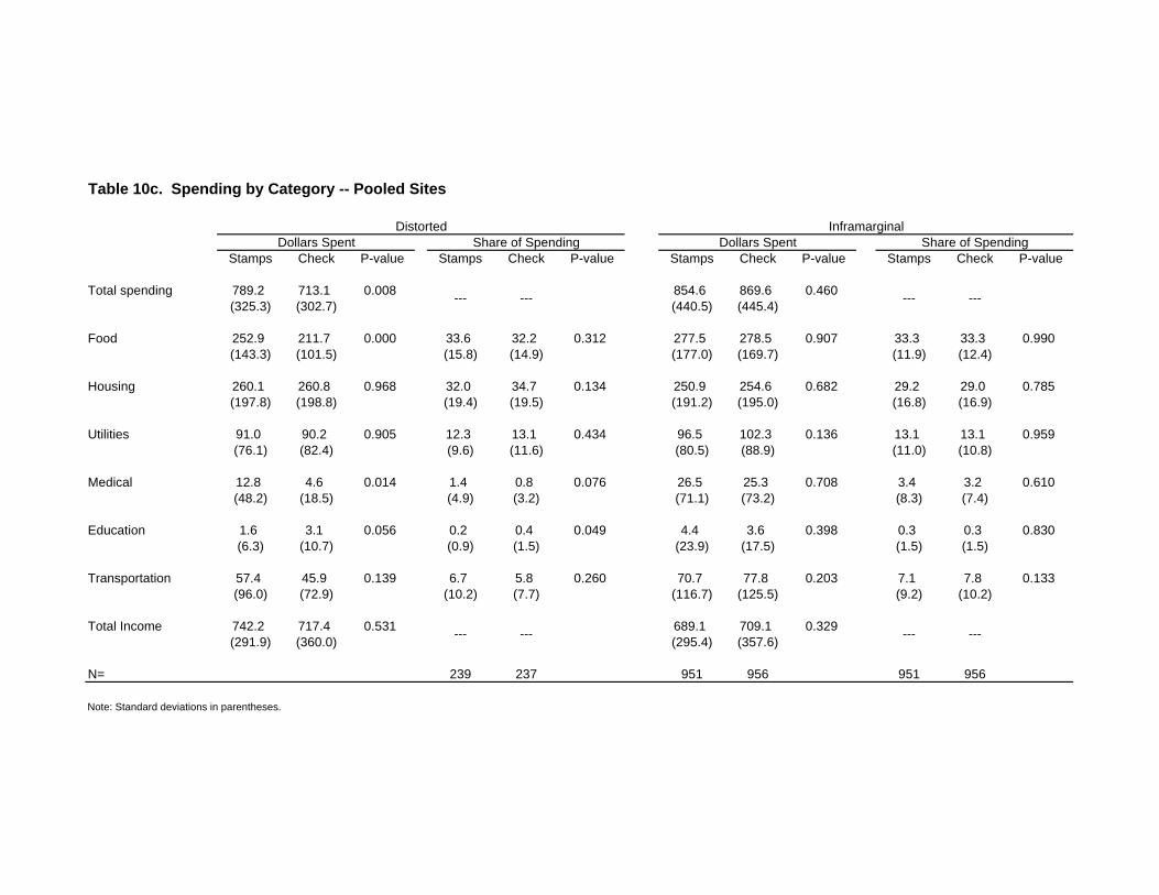
Table 10c. Spending by Category -- Pooled Sites

Stamps Check P-value Stamps Check P-value Stamps Check P-value Stamps Check P-value

Total spending 789.2 713.1 0.008 854.6 869.6 0.460(325.3) (302.7) (440.5) (445.4)

Food 252.9 211.7 0.000 33.6 32.2 0.312 277.5 278.5 0.907 33.3 33.3 0.990(143.3) (101.5) (15.8) (14.9) (177.0) (169.7) (11.9) (12.4)

Housing 260.1 260.8 0.968 32.0 34.7 0.134 250.9 254.6 0.682 29.2 29.0 0.785(197.8) (198.8) (19.4) (19.5) (191.2) (195.0) (16.8) (16.9)

Utilities 91.0 90.2 0.905 12.3 13.1 0.434 96.5 102.3 0.136 13.1 13.1 0.959(76.1) (82.4) (9.6) (11.6) (80.5) (88.9) (11.0) (10.8)

Medical 12.8 4.6 0.014 1.4 0.8 0.076 26.5 25.3 0.708 3.4 3.2 0.610(48.2) (18.5) (4.9) (3.2) (71.1) (73.2) (8.3) (7.4)

Education 1.6 3.1 0.056 0.2 0.4 0.049 4.4 3.6 0.398 0.3 0.3 0.830(6.3) (10.7) (0.9) (1.5) (23.9) (17.5) (1.5) (1.5)

Transportation 57.4 45.9 0.139 6.7 5.8 0.260 70.7 77.8 0.203 7.1 7.8 0.133(96.0) (72.9) (10.2) (7.7) (116.7) (125.5) (9.2) (10.2)

Total Income 742.2 717.4 0.531 689.1 709.1 0.329(291.9) (360.0) (295.4) (357.6)

N= 239 237 951 956 951 956

Note: Standard deviations in parentheses.

InframarginalDollars Spent Share of Spending

--- ---

Distorted

--- ---

Dollars Spent Share of Spending

--- --- --- ---

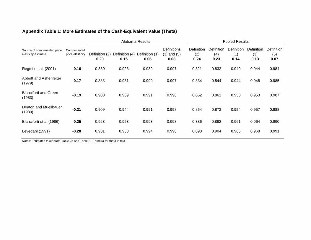
Appendix Table 1: More Estimates of the Cash-Equivalent Value (Theta)

Source of compensated price elasticity estimate

Compensated price elasticity Definition (2) Definition (4) Definition (1)

Definitions (3) and (5)

Definition (2)

Definition (4)

Definition (1)

Definition (3)

Definition (5)

0.20 0.15 0.06 0.03 0.24 0.23 0.14 0.13 0.07

Regmi et. al. (2001) -0.16 0.880 0.926 0.989 0.997 0.821 0.832 0.940 0.944 0.984

Abbott and Ashenfelter (1979)

-0.17 0.888 0.931 0.990 0.997 0.834 0.844 0.944 0.948 0.985

Blanciforti and Green (1983)

-0.19 0.900 0.939 0.991 0.998 0.852 0.861 0.950 0.953 0.987

Deaton and Muellbauer (1980)

-0.21 0.909 0.944 0.991 0.998 0.864 0.872 0.954 0.957 0.988

Blanciforti et al (1986) -0.25 0.923 0.953 0.993 0.998 0.886 0.892 0.961 0.964 0.990

Levedahl (1991) -0.28 0.931 0.958 0.994 0.998 0.898 0.904 0.965 0.968 0.991

Notes: Estimates taken from Table 2a and Table 3. Formula for theta in text.

Alabama Results Pooled Results

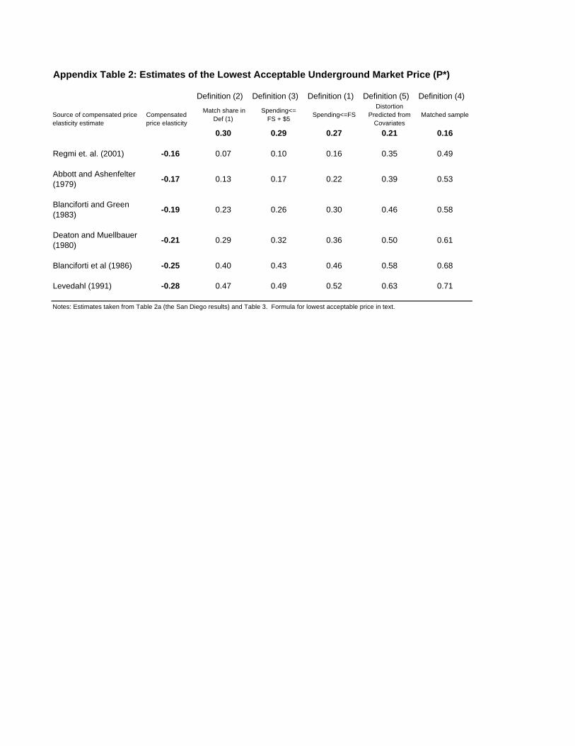
Appendix Table 2: Estimates of the Lowest Acceptable Underground Market Price (P*)

Definition (2) Definition (3) Definition (1) Definition (5) Definition (4)

Source of compensated price elasticity estimate

Compensated price elasticity

Match share in Def (1)

Spending<= FS + $5

Spending<=FSDistortion

Predicted from Covariates

Matched sample

0.30 0.29 0.27 0.21 0.16

Regmi et. al. (2001) -0.16 0.07 0.10 0.16 0.35 0.49

Abbott and Ashenfelter (1979)

-0.17 0.13 0.17 0.22 0.39 0.53

Blanciforti and Green (1983)

-0.19 0.23 0.26 0.30 0.46 0.58

Deaton and Muellbauer (1980)

-0.21 0.29 0.32 0.36 0.50 0.61

Blanciforti et al (1986) -0.25 0.40 0.43 0.46 0.58 0.68

Levedahl (1991) -0.28 0.47 0.49 0.52 0.63 0.71

Notes: Estimates taken from Table 2a (the San Diego results) and Table 3. Formula for lowest acceptable price in text.

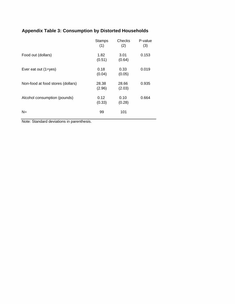
Appendix Table 3: Consumption by Distorted Households

Stamps Checks P-value(1) (2) (3)

Food out (dollars) 1.82 3.01 0.153(0.51) (0.64)

Ever eat out (1=yes) 0.18 0.33 0.019(0.04) (0.05)

Non-food at food stores (dollars) 28.38 28.66 0.935(2.96) (2.03)

Alcohol consumption (pounds) 0.12 0.10 0.664(0.33) (0.28)

N= 99 101

Note: Standard deviations in parenthesis.

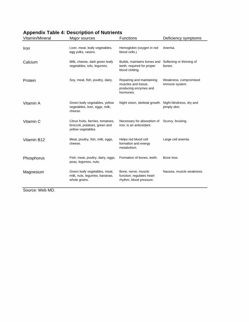
Appendix Table 4: Description of NutrientsVitamin/Mineral Major sources Functions Deficiency symptoms

Iron Liver, meat, leafy vegetables, egg yolks, raisins.

Hemoglobin (oxygen in red blood cells.)

Anemia.

Calcium Milk, cheese, dark green leafy vegetables, tofu, legumes.

Builds, maintains bones and teeth; required for proper blood clotting.

Softening or thinning of bones.

Protein Soy, meat, fish, poultry, dairy. Repairing and maintaining muscles and tissue, producing enzymes and hormones.

Weakness, compromised immune system.

Vitamin A Green leafy vegetables, yellow vegetables, liver, eggs, milk, cheese.

Night vision, skeletal growth. Night blindness, dry and pimply skin.

Vitamin C Citrus fruits, berries, tomatoes, broccoli, potatoes, green and yellow vegetables.

Necessary for absorption of iron; is an antioxidant.

Scurvy, bruising.

Vitamin B12 Meat, poultry, fish, milk, eggs, cheese.

Helps red blood cell formation and energy metabolism.

Large cell anemia.

Phosphorus Fish, meat, poultry, dairy, eggs, peas, legumes, nuts.

Formation of bones, teeth. Bone loss.

Magnesium Green leafy vegetables, meat, milk, nuts, legumes, bananas, whole grains.

Bone, nerve, muscle function; regulates heart rhythm, blood pressure.

Nausea, muscle weakness.

Source: Web MD.