What can we learn about solar activity from studying magnetogram evolution?

What can we learn about solar activity from studying magnetogram evolution?

Brian T. Welsch SSL, UC-Berkeley

I will briefly review results from recent studies of magnetic evolution in sequences of magnetograms, and discuss avenues for future research suggested by these results. Further work is necessary to understand both the physics underlying a recently identified photospheric flow - flare association, and how this association is related to other flare-associated phenomena, including vertical electric currents at the photosphere and subsurface flow properties and their evolution. Efforts to understand flare activity will be aided by improvements in techniques for estimating the electric fields that govern magnetic evolution in magnetograms, e.g., incorporating constraints from Doppler shifts and multi-height magnetic measurements. Electric field estimates can also be applied to several other problems, including understanding the ultimate fate of active region flux and time-dependent coronal magnetic field modeling.

Topics

I’ll begin by reviewing results from recent research.(i) flows & flares(ii) estimating magnetogram electric fields

Next, I’ll discuss ideas for research with the VSM. (iii) case studies of short-timescale evolution(iv) studies involving the “core” database

Flares and CMEs are powered by energy stored in electric currents in the coronal magnetic field Bcor.

From T.G. Forbes, “A Review on the Genesis of Coronal Mass Ejections”, JGR (2000)

What physical processes produce the electric currents that store energy in Bcor? Two options are:

• Currents could form in the interior, then emerge into the corona.

– Current-carrying magnetic fields have been observed to emerge (e.g., Leka et al. 1996, Okamoto et al. 2008)

• Photospheric evolution could induce currents in already-emerged coronal magnetic fields.

– From simple scalings, McClymont & Fisher (1989) argued induced currents would be too weak to power large flares

– Detailed studies by Longcope et al. (2007) and Kazachenko et al. (2009) suggest strong enough currents can be induced

General picture: slow buildup, sudden release.

If Bcor drives flares, why study magnetograms of the photospheric and chromospheric fields, Bph and Bch?

The coronal magnetic field Bcor powers flares and CMEs, but measurements of (vector) Bcor are rare and uncertain.

When not flaring, coronal magnetic evolution should be nearly ideal magnetic connectivity is preserved.

As the photospheric and chromospheric fields, Bph and Bch, evolve, changes in the coronal field Bcor are induced.

Further, following active region (AR) fields in time can provide information about their history and development.

9

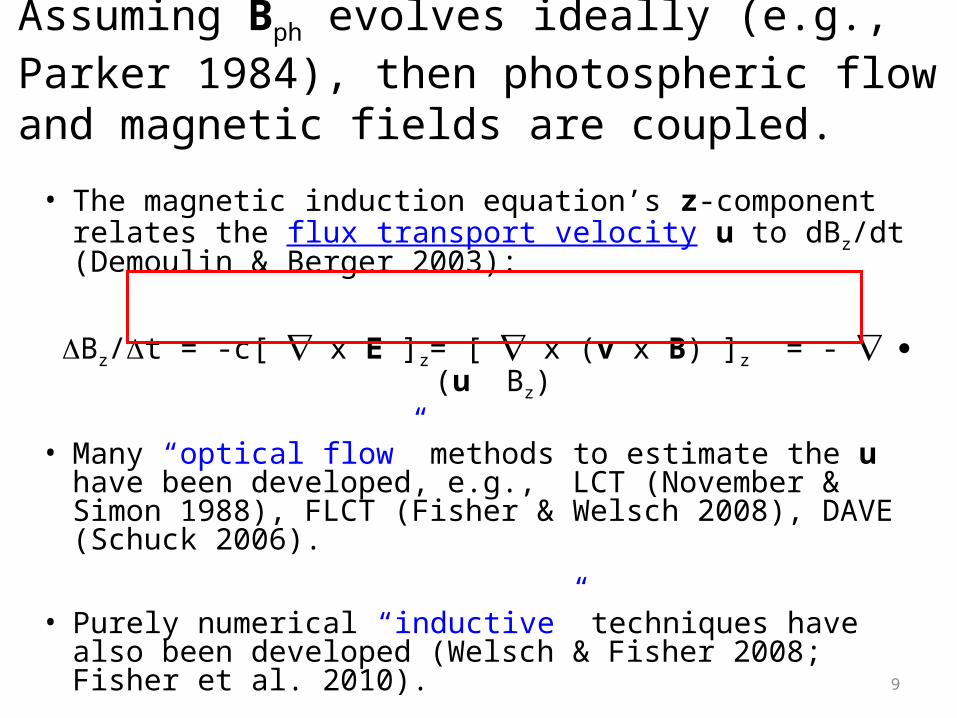
Assuming Bph evolves ideally (e.g., Parker 1984), then photospheric flow and magnetic fields are coupled.

• The magnetic induction equation’s z-component relates the flux transport velocity u to dBz/dt (Demoulin & Berger 2003):

Bz/t = -c[ x E ]z= [ x (v x B) ]z = - (u Bz)

• Many “optical flow” methods to estimate the u have been developed, e.g., LCT (November & Simon 1988), FLCT (Fisher & Welsch 2008), DAVE (Schuck 2006).

• Purely numerical “inductive” techniques have also been developed (Welsch & Fisher 2008; Fisher et al. 2010).

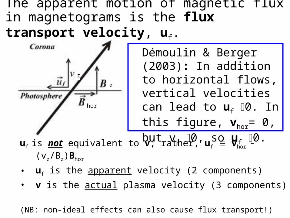
The apparent motion of magnetic flux in magnetograms is the flux transport velocity, uf.

uf is not equivalent to v; rather, uf vhor - (vz/Bz)Bhor

• uf is the apparent velocity (2 components)

• v is the actual plasma velocity (3 components)

(NB: non-ideal effects can also cause flux transport!)

Démoulin & Berger (2003): In addition to horizontal flows, vertical velocities can lead to uf 0. In this figure, vhor= 0, but vz 0, so uf 0.hor

z

z

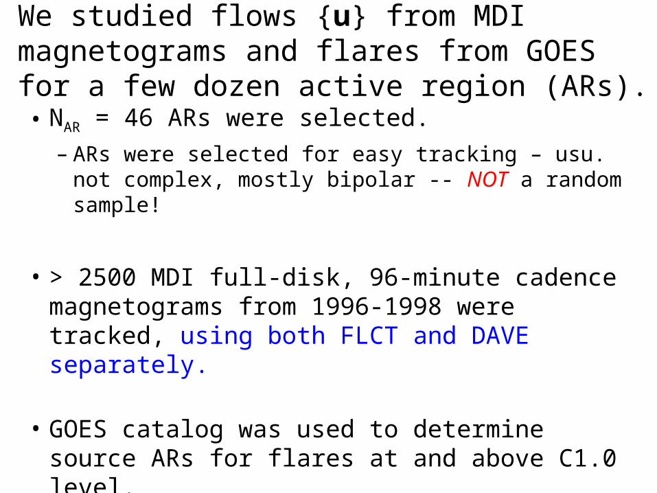
We studied flows {u} from MDI magnetograms and flares from GOES for a few dozen active region (ARs).

• NAR = 46 ARs were selected.– ARs were selected for easy tracking – usu. not

complex, mostly bipolar -- NOT a random sample!

• > 2500 MDI full-disk, 96-minute cadence magnetograms from 1996-1998 were tracked, using both FLCT and DAVE separately.

• GOES catalog was used to determine source ARs for flares at and above C1.0 level.

13

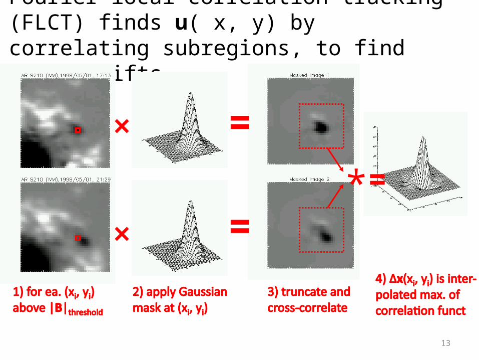
Fourier local correlation tracking (FLCT) finds u( x, y) by correlating subregions, to find local shifts.

*

=

==

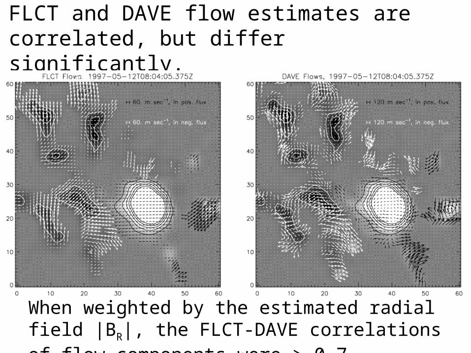
FLCT and DAVE flow estimates are correlated, but differ significantly.

When weighted by the estimated radial field |BR|, the FLCT-DAVE correlations of flow components were > 0.7.

For each magnetogram and flow estimate, we computed several properties of BR and u, e.g.,

- average unsigned field |BR| - summed unsigned flux, = Σ |BR| da2

- summed flux near strong-field PILs, R (Schrijver 2007)- sum of field squared, Σ BR

2

- rates of change d/dt and dR/dt - summed speed, Σ u.- averages and sums of divergences (h · u), (h · u BR)

- averages and sums of curls (h x u), (h x u BR)

- the summed “proxy Poynting flux,” SR = Σ u BR2

(and many more!)

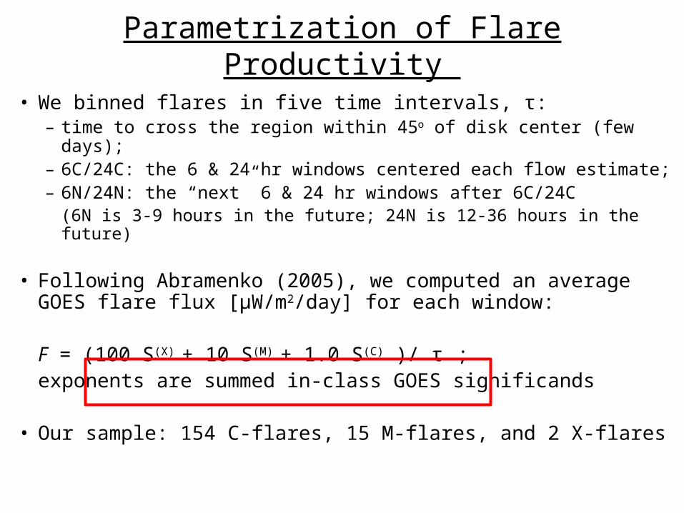
Parametrization of Flare Productivity

• We binned flares in five time intervals, τ: – time to cross the region within 45o of disk center (few days);– 6C/24C: the 6 & 24 hr windows centered each flow estimate;– 6N/24N: the “next” 6 & 24 hr windows after 6C/24C

(6N is 3-9 hours in the future; 24N is 12-36 hours in the future)

• Following Abramenko (2005), we computed an average GOES flare flux [μW/m2/day] for each window:

F = (100 S(X) + 10 S(M) + 1.0 S(C) )/ τ ;exponents are summed in-class GOES significands

• Our sample: 154 C-flares, 15 M-flares, and 2 X-flares

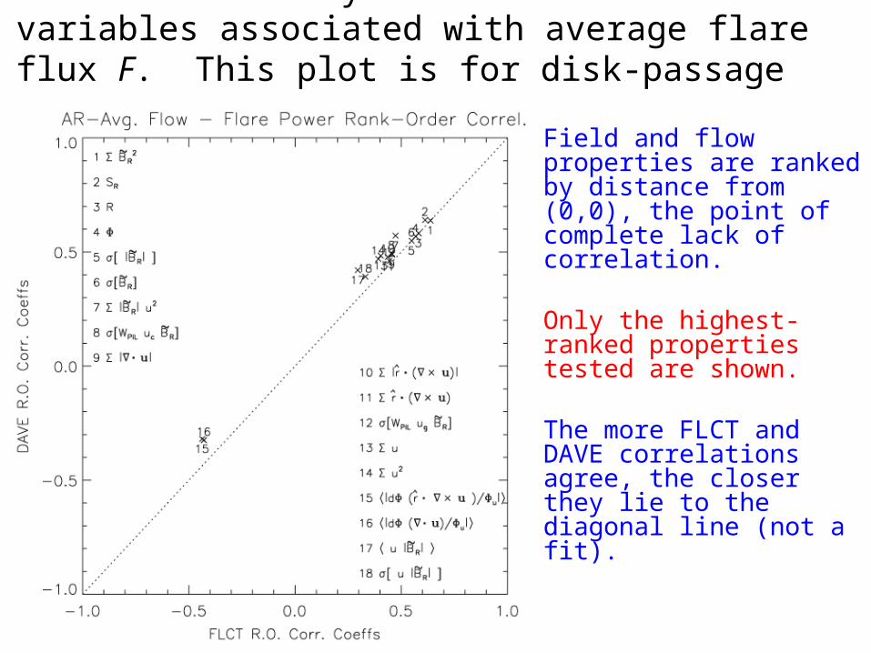
Correlation analysis showed several variables associated with average flare flux F. This plot is for disk-passage averages.

Field and flow properties are ranked by distance from (0,0), the point of complete lack of correlation.

Only the highest-ranked properties tested are shown.

The more FLCT and DAVE correlations agree, the closer they lie to the diagonal line (not a fit).

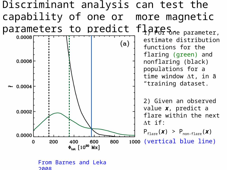
Discriminant analysis can test the capability of one or more magnetic parameters to predict flares.

1) For one parameter, estimate distribution functions for the flaring (green) and nonflaring (black) populations for a time window t, in a “training dataset.”

2) Given an observed value x, predict a flare within the next t if:

Pflare(x) > Pnon-

flare(x)

(vertical blue line) From Barnes and Leka 2008

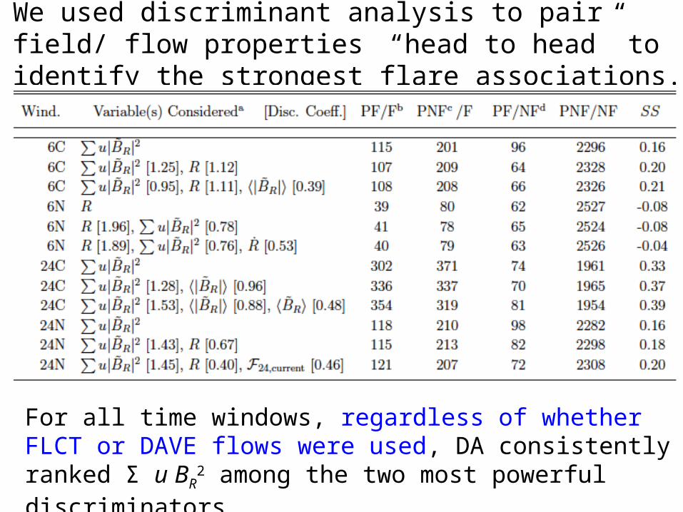
We used discriminant analysis to pair field/ flow properties

“head to head” to identify the strongest flare associations.

For all time windows, regardless of whether FLCT or DAVE flows were used, DA consistently ranked Σ u BR

2 among the two most powerful discriminators.

Physically, why is the proxy Poynting flux, SR = Σ uBR2,

associated with flaring? Open questions:Why should u BR

2 – part of the horizontal Poynting flux from Eh x Br – matter for flaring? – The vertical Poynting flux, due to Eh x Bh, is presumably primarily

responsible for injecting energy into the corona. – (Another component of the horizontal Poynting flux, from

Er x Bh, was neglected in our analysis. Is it also significant?)

– With Bh available from vector magnetograms, these questions can be addressed!

• Do flows from flux emergence or rotating sunspots also produce large values of u BR

2?

• How is u BR2 related to flare-associated subsurface flow

properties (e.g., Komm & Hill 2009; Reinard et al. 2010)?

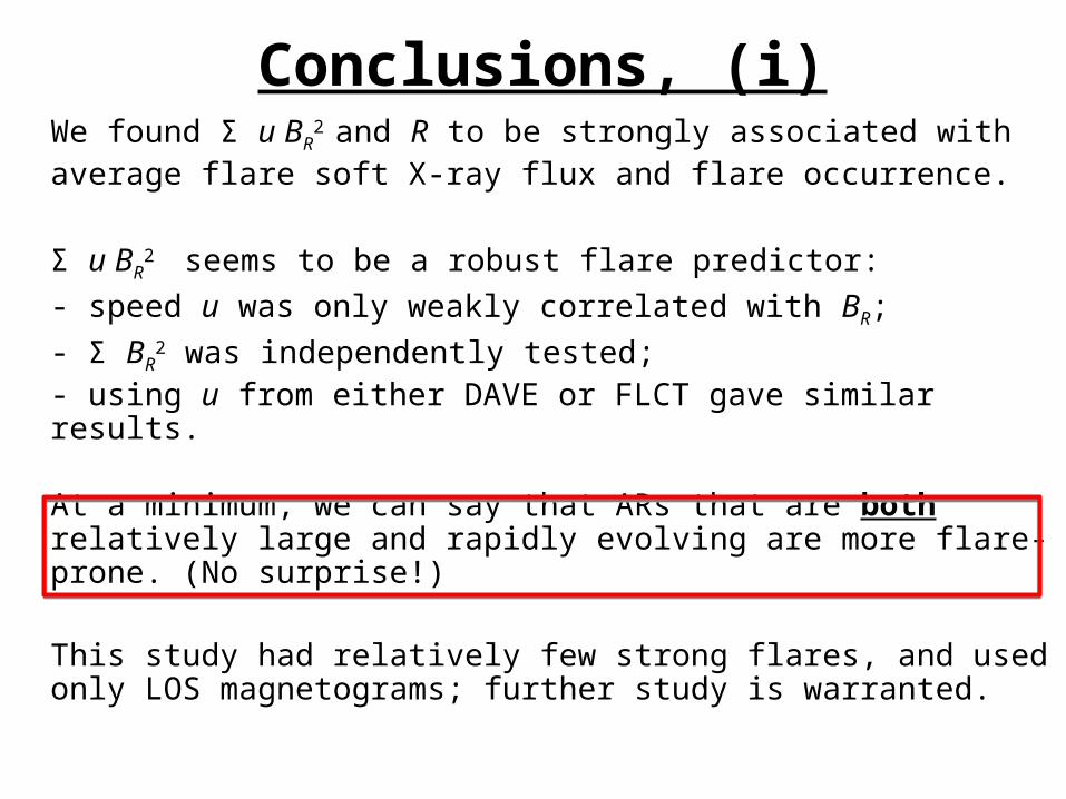
Conclusions, (i)We found Σ u BR

2 and R to be strongly associated with average flare soft X-ray flux and flare occurrence.

Σ u BR2 seems to be a robust flare predictor:

- speed u was only weakly correlated with BR; - Σ BR

2 was independently tested;- using u from either DAVE or FLCT gave similar results.

At a minimum, we can say that ARs that are both relatively large and rapidly evolving are more flare-prone. (No surprise!)

This study had relatively few strong flares, and used only LOS magnetograms; further study is warranted.

Topics



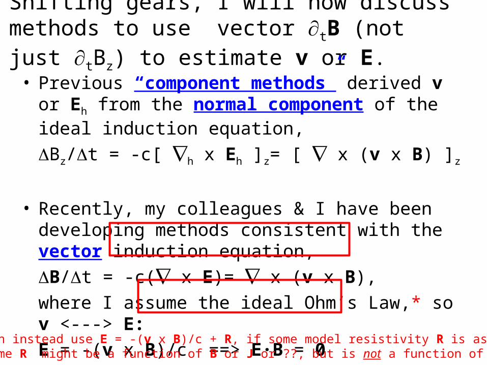
Shifting gears, I will now discuss methods to use vector tB (not just tBz) to estimate v or E.

• Previous “component methods” derived v or Eh from the normal component of the ideal induction equation,

Bz/t = -c[ h x Eh ]z= [ x (v x B) ]z

• Recently, my colleagues & I have been developing methods consistent with the vector induction equation,

B/t = -c( x E)= x (v x B),where I assume the ideal Ohm’s Law,* so v <---> E:

E = -(v x B)/c ==> E·B = 0

*One can instead use E = -(v x B)/c + R, if some model resistivity R is assumed.(I assume R might be a function of B or J or ??, but is not a function of E.)

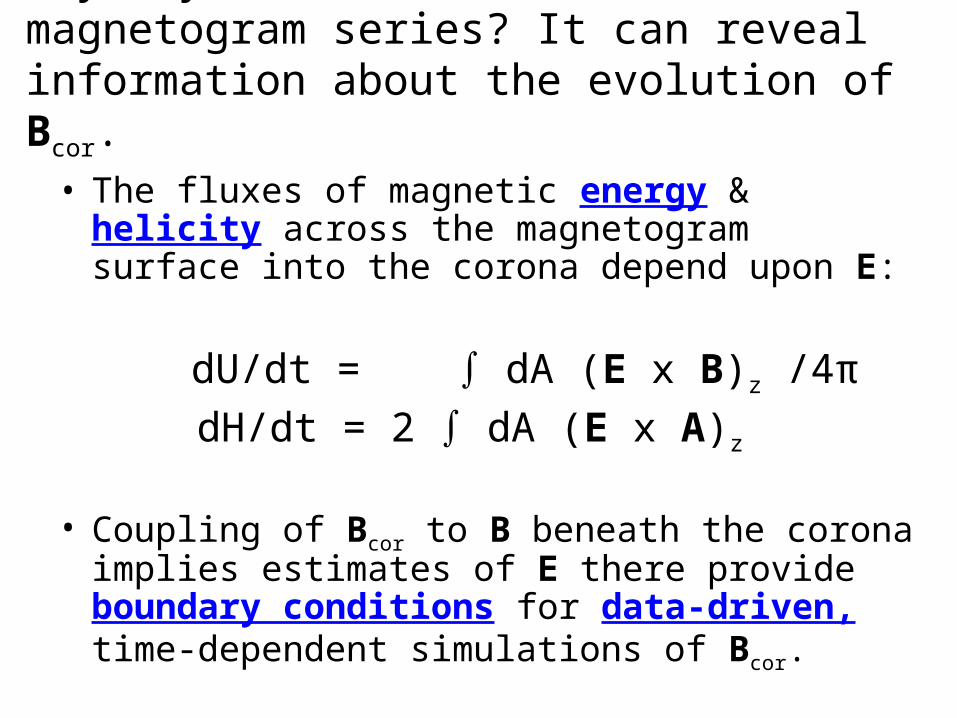
Why try to estimate E from magnetogram series? It can reveal information about the evolution of Bcor.

• The fluxes of magnetic energy & helicity across the magnetogram surface into the corona depend upon E:

dU/dt = ∫ dA (E x B)z /4π

dH/dt = 2 ∫ dA (E x A)z

• Coupling of Bcor to B beneath the corona implies estimates of E there provide boundary conditions for data-driven, time-dependent simulations of Bcor.

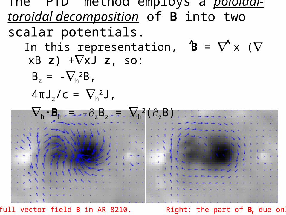
The “PTD” method employs a poloidal-toroidal decomposition of B into two scalar potentials.

In this representation, B = x ( xB z) +xJ z, so:Bz = -h

2B,

4πJz/c = h2J,

h·Bh = -zBz = h2(zB)

Left: the full vector field B in AR 8210. Right: the part of Bh due only to J.

^ ^

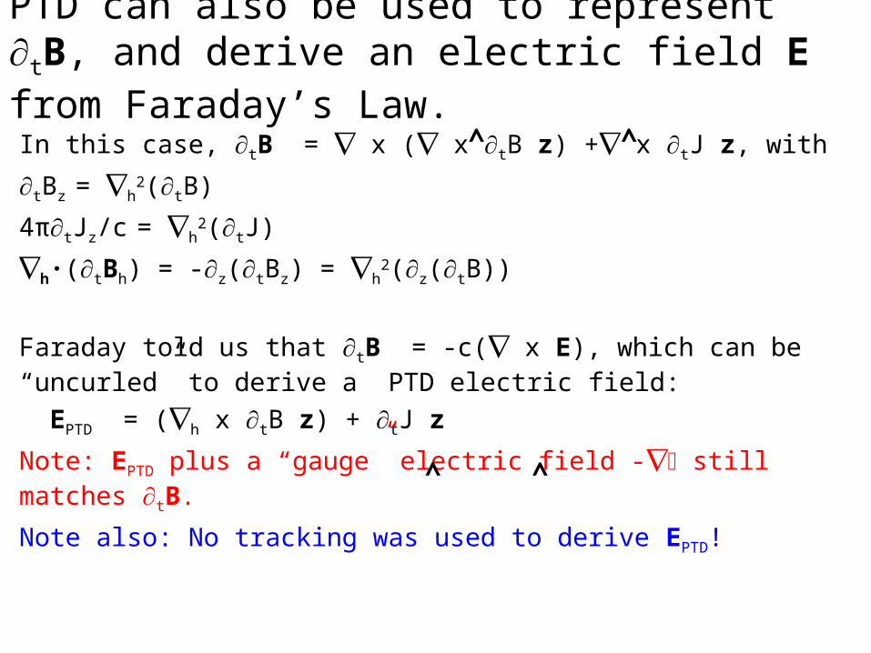
PTD can also be used to represent tB, and derive an electric field E from Faraday’s Law.

In this case, tB = x ( x tB z) + x tJ z, with

tBz = h2(tB)

4πtJz/c = h2(tJ)

h·(tBh) = -z(tBz) = h2(z(tB))

Faraday told us that tB = -c( x E), which can be “uncurled” to derive a PTD electric field:

EPTD = (h x tB z) + tJ z

Note: EPTD plus a “gauge” electric field - still matches tB.

Note also: No tracking was used to derive EPTD!

^

^ ^

^

The E derived via PTD uses only tB, so EPTD·B ≠ 0. Hence, we must solve for (x,y) so (EPTD - )·B = 0.

I have developed a practical iterative approach: 1. Define b = unit vector along B2. Define = s1(x, y) b + s2(x, y)(z x b) + s3(x, y) b x (z x b)

3. Set s1(x, y) = EPTD· b

4. Solve h2 = h· [s1(x,y)bh + s2(x, y)(z x b) − s3(x, y)bzbh]

5. Update s2 = z·(bhx )/bh2 and s3 = z -(bh· ) bz/bh

2

6. Repeat steps 4 & 5 until convergence.

This approach quickly yields a solution.

However, uniqueness is still a problem: any (x,y)satisfying ·B = 0 can be added to this solution! For (many) more details about PTD, see Fisher et al. 2010.

^

^

^

^

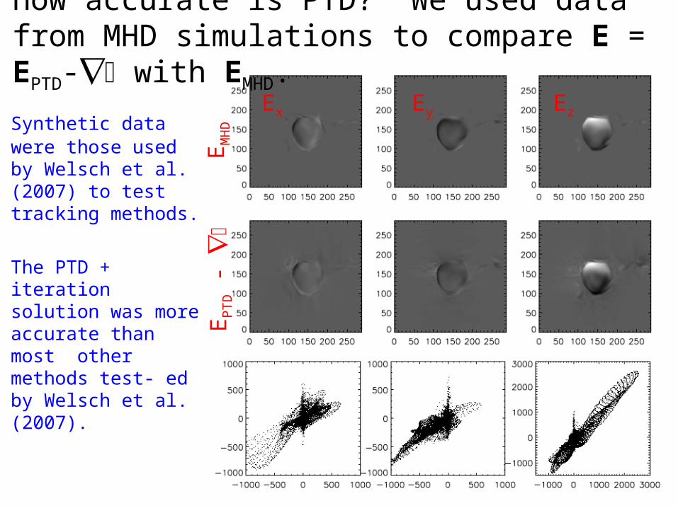
How accurate is PTD? We used data from MHD simulations to compare E = EPTD- with EMHD.

Synthetic data were those used by Welsch et al. (2007) to test tracking methods.

The PTD + iteration solution was more accurate than most other methods tested by Welsch et al. (2007).

Ex Ey Ez

EP

TD -

EM

HD

While tB provides more information about E than tBz alone, it still does not fully determine E.

1. Faraday’s Law only relates tB to the curl of E, not E itself; the gauge electric field is unconstrained by tB.

(We used Ohm’s Law as an additional constraint.)

2. tBh also depends upon vertical derivatives in Eh, which single-height magnetograms do not fully constrain.

1. Additional observational data must be used to obtain more information about both of these unknowns.

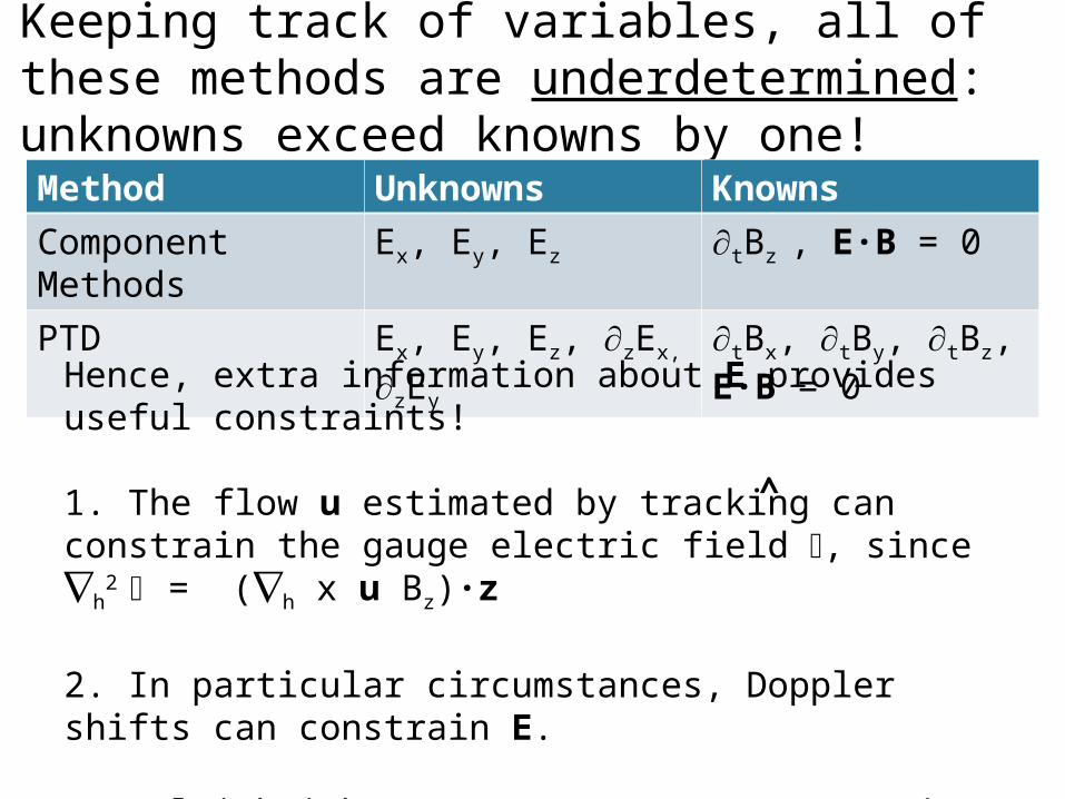
Keeping track of variables, all of these methods are underdetermined: unknowns exceed knowns by one!

Method Unknowns KnownsComponent Methods Ex, Ey, Ez tBz , E·B = 0

PTD Ex, Ey, Ez, zEx, zEy tBx, tBy, tBz, E·B = 0

Hence, extra information about E provides useful constraints!

1. The flow u estimated by tracking can constrain the gauge electric field , since h

2 = (h x u Bz)·z

2. In particular circumstances, Doppler shifts can constrain E.

3. Multi-height magnetograms can constrain zEh.

(Given noise in the data, overdetermining E is fine!)

^

1. Tracking with “component methods” constrains by estimating u in the source term (h x u Bz) · z.

Methods to find via tracking include, e.g.: – Local Correlation Tracking (LCT, November & Simon 1988;

ILCT, Welsch et al. 2004; FLCT Fisher & Welsch 2008)– the Differential Affine Velocity Estimator (DAVE, and

DAVE4VM; Schuck 2006 & Schuck 2008)

(Methods to find via integral constraints also exist, e.g., Longcope’s [2004] Minimum Energy Fit [MEF] method.)

Welsch et al. (2007) tested some of these methods using “data” from MHD simulations; MEF performed best. Further tests with more realistic data are underway.

^

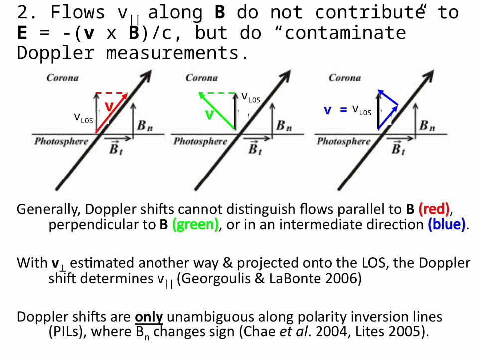
2. Flows v|| along B do not contribute to E = -(v x B)/c, but do “contaminate” Doppler measurements.

vLOSvLOS

vLOSv v v =

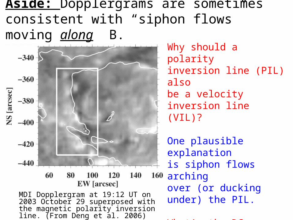
Aside: Dopplergrams are sometimes consistent with “siphon flows” moving along B.

MDI Dopplergram at 19:12 UT on 2003 October 29 superposed with the magnetic polarity inversion line. (From Deng et al. 2006)

Why should a polarity inversion line (PIL) also be a velocity inversion line (VIL)?

One plausible explanationis siphon flows arching over (or ducking under) the PIL.

What’s the DC Doppler shift along this PIL? Is flux emerging or submerging?

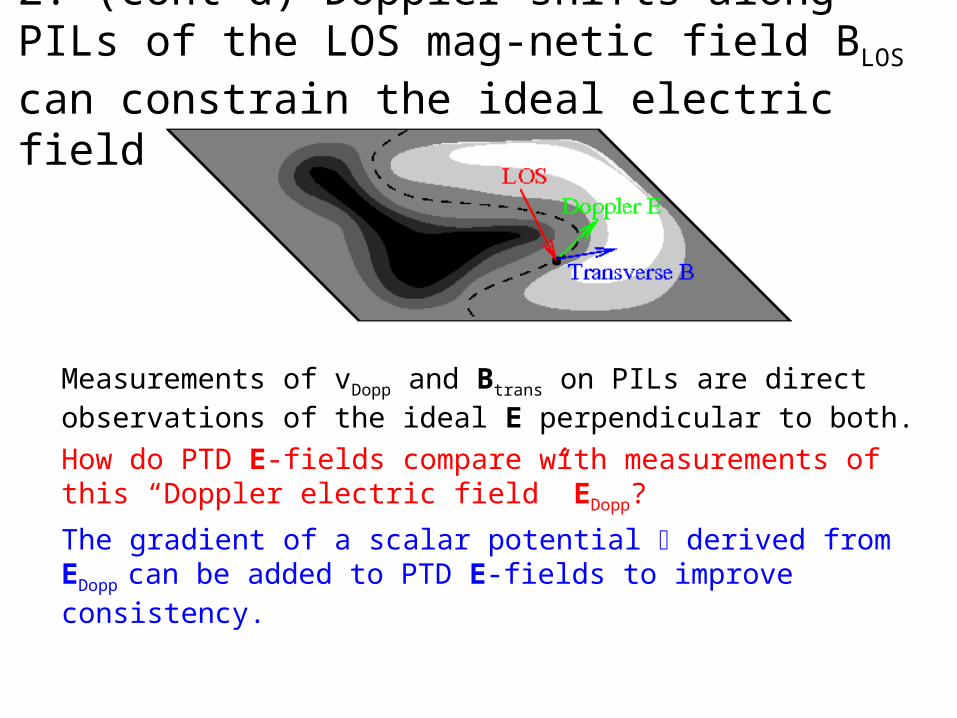
2. (cont’d) Doppler shifts along PILs of the LOS mag-netic field BLOS can constrain the ideal electric field E.

Measurements of vDopp and Btrans on PILs are direct observations of the ideal E perpendicular to both.How do PTD E-fields compare with measurements of this “Doppler electric field” EDopp?

The gradient of a scalar potential derived from EDopp can be added to PTD E-fields to improve consistency.

Bh(ti)

v

Bh(tf)v Bh(tf)

Bh(ti)

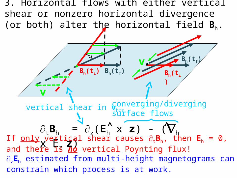
tBh = z(Eh x z) - (h x Ez z)

vertical shear in vhor

^

converging/diverging surface flows

3. Horizontal flows with either vertical shear or nonzero horizontal divergence (or both) alter the horizontal field Bh.

^

If only vertical shear causes tBh, then Eh = 0, and there is no vertical Poynting flux!zEh estimated from multi-height magnetograms can constrain which process is at work.

• The PTD method determines an electric field E consistent with vector magnetic evolution, tB.

– Previous “component” methods (e.g., ILCT, FLCT, DAVE, DAVE4VM, MEF) were consistent with tBz.

– Faraday’s Law implies that tB alone does not fully specify E – there is an undetermined “gauge” electric field .

• Tracking can help constrain h.

• Flows perpendicular to B contribute to E, and Doppler shifts along PILs constrain perp. flows, so also constrain E.

• Eh derived from multi-height magnetograms can constrain zEh.

Conclusions, (ii)

Topics



Shifting gears yet again, I present a few ideas (I have more!) for research projects with SOLIS / VSM.

• Many projects I envision involve VSM observations in “campaign mode.” – That is, obtaining sequences magnetograms at higher

cadence than the “core data rate” of 3 per day.– HMI will also record photospheric vector magneto-

grams; SOLIS data should complement (not “compete”).

• I would value input from NSO collaborators about prioritization.

• This presentation of my ideas is terse and cursory.So please interrupt me to ask questions!

Project #1: Estimate Poynting fluxes, and compare with both the proxy Poynting flux and flare activity.

• Welsch et al. (2009) had only LOS magnetograms, so could only estimate a “proxy Poynting flux”, (Eh x BR)

• With vector magnetograms, the vertical Poynting flux can be estimated, (Eh x Bh)– the full horizontal flux can also be estimated

• How are these quantities correlated in space and time? – For a sample of active region magnetogram sequences, how

are these energy fluxes related to flare activity?

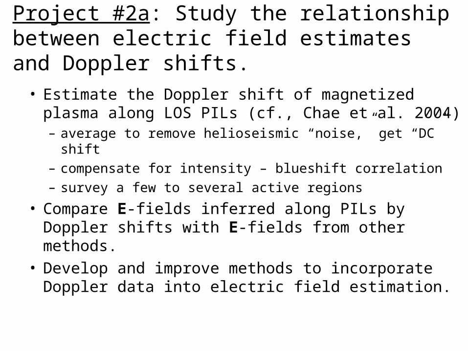
Project #2a: Study the relationship between electric field estimates and Doppler shifts.

• Estimate the Doppler shift of magnetized plasma along LOS PILs (cf., Chae et al. 2004)– average to remove helioseismic “noise,” get “DC” shift– compensate for intensity – blueshift correlation– survey a few to several active regions

• Compare E-fields inferred along PILs by Doppler shifts with E-fields from other methods.

• Develop and improve methods to incorporate Doppler data into electric field estimation.

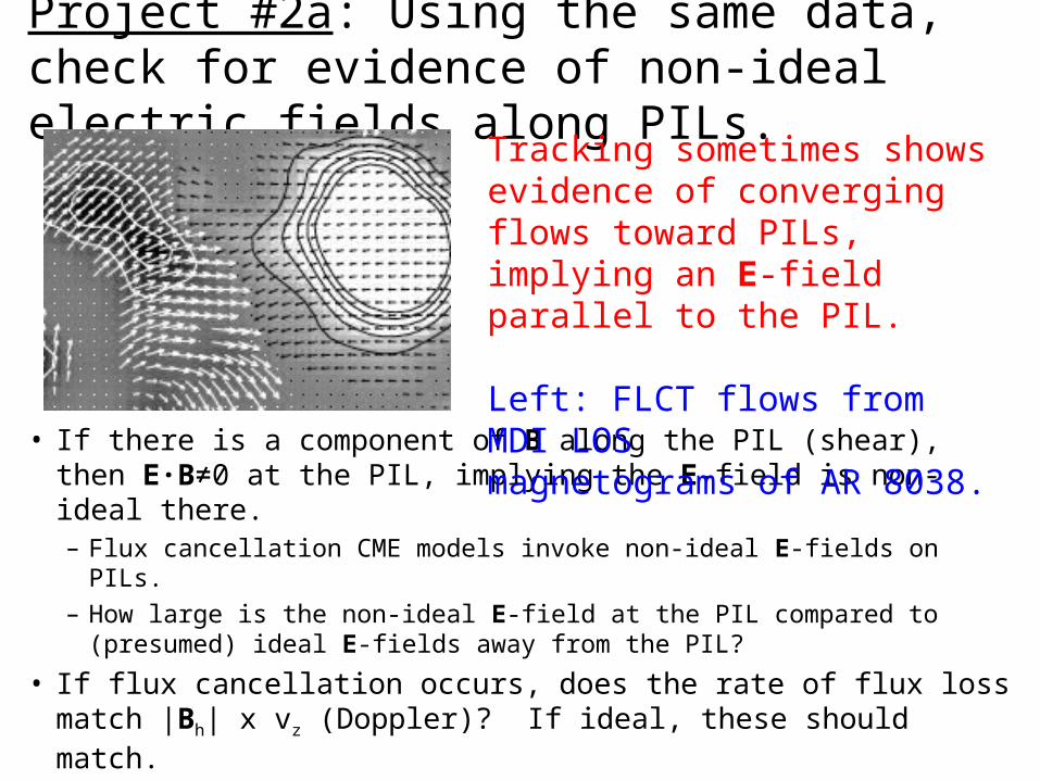
Project #2a: Using the same data, check for evidence of non-ideal electric fields along PILs.

• If there is a component of B along the PIL (shear), then E·B≠0 at the PIL, implying the E-field is non-ideal there. – Flux cancellation CME models invoke non-ideal E-fields on PILs. – How large is the non-ideal E-field at the PIL compared to

(presumed) ideal E-fields away from the PIL?

• If flux cancellation occurs, does the rate of flux loss match |Bh| x vz (Doppler)? If ideal, these should match.

Tracking sometimes shows evidence of converging flows toward PILs, implying an E-field parallel to the PIL.

Left: FLCT flows from MDI LOS magnetograms of AR 8038.

Project #3: Study electric fields in multi-height magnetogram sequences.

• Estimate E in sequences magnetograms in spectral lines with different formation heights– chromosph. LOS & vector photosph., SOLIS 854.2nm + HMI – (also worthwhile to baseline SOLIS & HMI photospheric)

• Compare electric fields / flows.– Where are they correlated in space? Where are they not? (e.g., in

strong field vs. weak field regions?)– Do flow vorticities / divergences appear in common loci?– Do flows decorrelate on similar timescales?

• Inversions of the chromospheric vector field would certainly be useful, but also certainly not necessary.

Are changes in vertical currents associated with flow vorticity? Do sunspot rotations tend to increase or decrease currents?

Are shearing or converging motions statistically stronger where increases in magnetic shear occur?

Project #4: What is the relationship between flows and evolution of magnetic structure?

The component of Bh that arises purely from currents (derived using PTD), from a SOLIS/ VSM magnetogram of AR 10961. How do flows affect these structures?

Topics



Project #5: Compare chromospheric magnetic prop-erties with RHESSI hard X-ray (HXR) flare emission.

• HXR emission is bremsstrahlung from non-thermal particles precipitating onto the upper chromosphere.

• Magnetic mirroring is thought to govern the precipitation of flare particles. – If so, in magnetic fields that converge more strongly, more

particles should mirror, and less HXR emission should be seen.

• Models of the potential magnetic field at the chromo-sphere (from SOLIS data) quantify field convergence.

• HXR intensities & indices of power-law fits to emission spectra can be compared to aspects of chromospheric B.

(In collaboration with SSL’s Jim McTiernan & Pascal Saint-Hilaire.)

• Using LOS magnetograms, we found a “proxy Poynting flux,” SR = Σ uBR

2 to be related to flare activity.– It will be interesting to compare the “proxy” Poynting flux

with the Poynting flux from vector magnetogram sequences! • We developed the poloidal-toroidal decomposition

(PTD) method to determine an electric field E consistent with vector magnetic evolution, tB. – The method is in its infancy, and I look forward to applying it

to more vector magnetogram sequences!

• I presented several research ideas for SOLIS/VSM data.– I hope you don’t think they’re too crackpot!

Conclusions, final

• The PTD method determines an electric field E consistent with vector magnetic evolution, tB. The method is in its infancy, and I look forward to applying it to vector magnetogram sequences.

– Previous “component” methods (e.g., ILCT, FLCT, DAVE, DAVE4VM, MEF) were consistent with tBz.

– Faraday’s Law implies that tB alone does not fully specify E – there is an undetermined “gauge” electric field .

• Tracking can help constrain h.

• Flows perpendicular to B contribute to E, and Doppler shifts along PILs constrain perp. flows, so also constrain E.

• Eh derived from multi-height magnetograms can constrain zEh.

Conclusions, (ii)

Documents

What can we learn about solar activity from studying magnetogram evolution?