WHAT DETERMINES ENTREPRENEURIAL CLUSTERS? · · 2011-03-15To answer these questions, ... In this paper we extend the Lucas model to investigate two potential explanations ... Guiso

WHAT DETERMINES ENTREPRENEURIALCLUSTERS?

Luigi GuisoEuropean University Institute andEinaudi Institute for Economicsand Finance

Fabiano SchivardiUniversity of Cagliari andEinaudi Institute for Economicsand Finance

AbstractWe contrast two potential explanations of the substantial differences in entrepreneurial activityobserved across geographical areas: entry costs and external effects. We extend the Lucas model ofentrepreneurship to allow for heterogeneous entry costs and for externalities that shift the distributionof entrepreneurial talents. We show that these assumptions have opposite predictions on the relationbetween entrepreneurial activity and firm-level TFP: with different entry costs, in areas with moreentrepreneurs firms’ average productivity should be lower; with heterogeneous external effects itshould be higher. We test these implications on a sample of Italian firms and unambiguously rejectthe entry costs explanation in favor of the externalities explanation. We also investigate the sourcesof external effects, finding robust evidence that learning externalities are an important determinantof cross-sectional differences in entrepreneurial activity. (JEL: D24, D62, J23)

1. Introduction

There is a vast literature linking a country’s endowment of “entrepreneurship”with economic prosperity. Environments where entrepreneurs can emerge easily arepropitious to the creation of firms, their growth and their success. These ideas dateback to Marshall (1890) and Schumpeter (1911). For example, the latter sees theentrepreneur as the carrier of innovation and hence the true engine of growth. But ifentrepreneurship is so central to economic development, what drives it? Why are thereso many entrepreneurs in some areas, such as Silicon Valley, and so few in others? Dothese differences simply reflect differences in opportunities driven by, say, the presenceof Stanford University? Why do we find these clusters in some countries rather than

The editor in charge of this paper was Jordi Gali.

Acknowledgments: This paper has greatly benefited from repeated discussions with Luigi Zingales. Wethank Marianne Bertrand, Andrea Brandolini, Antonio Ciccone, Boyan Jovanovic, Riccardo Lagos, ClaudioMichelacci, Gianluca Violante, Ekaterina Zhuravskaya, two anonymous referees, the editor, participantsat the Workshop “Entry, Entrepreneurship and Financial Development” at the World Bank, the conference“Understanding Productivity Differences Across Sectors, Firms and Countries” in Alghero, and seminarparticipants at the Bank of Italy, Brick-Collegio Carlo Alberto, CEMFI, European University Institute, NewYork University, University of Turin, and Yale University for useful suggestions. Marco Chiurato and ElenaGenito provided outstanding research assistance. Luigi Guiso thanks the EEC and MURST and FabianoSchivardi the European Community’s Seventh Framework Programme (grant agreement no. 216813) forfinancial support. We are solely responsible for any mistakes. Both authors are CEPR members.E-mail: [email protected] (Guiso); [email protected] (Schivardi)

Journal of the European Economic Association February 2011 9(1):61–86c© 2010 by the European Economic Association DOI: 10.1111/j.1365-2966.2010.01006.x

62 Journal of the European Economic Association

others, and in particular areas within countries, such as in the Italian industrial districtsor the Ruhr? These important questions have often been in the forefront of policydebate and government intervention.

To answer these questions, one must address the choice of becoming anentrepreneur. Perhaps the best known model of entrepreneurship is that of Lucas(1978), explaining who in a given population will become an entrepreneur usingdifferences in exogenously given individual talents. In Lucas, “talent” is identifiedwith the ability to extract output from a given combination of inputs. Thus, moretalented individuals are those who can obtain a higher total factor productivity (TFP)if they start a business. Since individuals with more talent make more profits, theywill choose to be entrepreneurs. But what can explain clusters if we do not believein genetic differences, i.e., if the distribution at birth of individual ability is the sameacross populations?

In this paper we extend the Lucas model to investigate two potential explanationsof differences in entrepreneurial density across locations: entry costs and externaleffects. One possibility is that there are heterogeneous costs of entry, and the locationswith lower costs of setting up a firm end up with more entrepreneurs and more firmsbecause even relatively less talented individuals will find it profitable to start a businessthere. This is the approach implicitly followed by the large literature that focusses onfactors—particularly financial—that keep the would-be entrepreneur from actuallycreating a new firm. Banerjee and Newman (1994), for instance, show that creditconstraints can lead to poverty traps since potential entrepreneurs cannot invest inprofitable occupations involving set-up costs. It is well documented empirically thatlimited access to financial markets can hinder the emergence of entrepreneurs.1 Morerecently it has also been shown that regulation-induced high costs of entry hamperfirm and employment creation (Bertrand and Kramarz 2002; Fonseca, Lopez-Garcia,and Pissarides 2001; Klapper, Laeven, and Rajan 2006).

The second possibility is that the distribution of individual productivity is shifted bylocal factors, for instance because of differences in learning opportunities, knowledgespillovers or intermediate input variety. A vast body of literature has pointed out thatlocal externalities are an important determinant of firms’ performance.2 Externalitiescan be introduced in the Lucas model as shifters of the distribution of talents that makeindividuals more productive on average and therefore increase the share of agents thatchoose to start a business.

We show that the two assumptions have very different implications regardingthe relation between the propensity of individuals to become entrepreneurs and their

1. Evans and Jovanovic (1989) show that wealthier individuals who are currently employees are morelikely than the less wealthy to become self-employed, a finding consistent with liquidity constraints.Blanchflower and Oswald (1998) show that liquidity constraints affect the decision to become anentrepreneur even after controlling for individual ability. More recently, Guiso, Sapienza and Zingales(2004a) using individual level data for Italy find that in areas with a higher degree of financial developmentit is more likely that individuals become entrepreneurs, the rate of firm creation is higher, and there aremore firms per inhabitant.2. See for example the contributions in the Handbook of Regional and Urban Economics, Vol. 4(Henderson and Thisse 2004).

Guiso and Schivardi What Determines Entrepreneurial Clusters? 63

average productivity. Under entry costs differences, in areas with lower entry costs (i)there should be more entrepreneurs and, (ii) their firms’ average TFP should be lower.Thus, in equilibrium there should be a negative correlation between firm density in agiven location and their TFP. On the contrary, with externality differences, in placeswith stronger externalities average entrepreneurial ability is higher and there are moreentrepreneurs. In contrast to heterogeneous entry costs, the model with heterogeneousexternalities implies therefore that in equilibrium there should be a positive correlationbetween the share of entrepreneurs in a given location and their firms’ TFP.

We test these implications on a sample of Italian firms belonging to differentclusters. There is substantial evidence that Italian entrepreneurs are very likely tostart a business in the area where they were born, while workers are more mobile(Michelacci and Silva 2007). We therefore define actual entrepreneurs as firms activein a given location, potential entrepreneurs as individuals born in such location, andconstruct “entrepreneurial incidence” (EI) as the ratio of these two variables. We findthat the data unambiguously reject the entry costs story and support the externalitystory: areas with a higher EI are characterized by a higher average productivity. Moregenerally, a higher EI goes together with a rightward shift of the ability distribution.We also find that a firm’s TFP is positively correlated not only with the overall EI(that is, computed using the total number of active firms), but also with sectoral EI(computed using the active firms at the sectoral level). This is further evidence in favorof externalities, which are well known to have a strong sectoral character (Cingano andSchivardi 2004). This should not lead to the conclusion that entry costs are necessarilythe same across locations and play no role. Rather, (i) alone they cannot explaindifferences in entrepreneurial density and (ii) differences in shifters of the distributionof entrepreneurial talents are required to account for the pattern in the data.

Based on these results, in the reminder of the paper we corroborate theinterpretation of the positive correlation between density and quality in termsof externalities. Following Marshall (1890) and the literature on agglomerationeconomies, and in particular Duranton and Puga (2004), we identify three differentchannels through which agglomeration may affect firms’ productivity: first, theopportunities to learn from other firms, either because of knowledge spillovers orthrough learning entrepreneurial abilities from the observation of other firms; second,the size of the local work force, which can increase the division of labor and thequality of job–worker matches; and third, a greater variety of intermediate inputs.To discriminate between these three sources of externalities we run a horse race byconstructing proxies for each one, computed at the local-sectoral level. As a proxyfor learning opportunities and knowledge spillovers we use the number of firms ina location, the idea being that more firms offer more learning points; we proxy job-matching opportunities with the size of the local workforce; intermediate inputs varietyis measured by the ratio of intermediate inputs to value added at the local level. Wefind strong evidence for the first channel, supporting evidence for intermediate inputsvariety, and very weak or no evidence for externalities generated by labor pooling.In fact, the correlation between TFP and the number of firms proves to be extremelyrobust to a variety of controls. We further corroborate our interpretation of the number


of firms in terms of learning and knowledge spillovers. Following an idea of Cicconeand Hall (1996), to address potential endogeneity concerns we instrument the numberof firms with the local population in 1861, obtaining very similar estimates to the OLSones.

This paper relates to three strands in the literature. First, it is connected withthe entrepreneurship literature: we sort out two alternative explanations of clusters.Second, it contributes to the agglomeration literature: we investigate the sources of localexternalities. Finally, it is related to the productivity literature: we provide evidencethat differences in firm-level TFP may be due to the differing ability of entrepreneurs,which in turn could depend on the degree of learning spillovers.

Our results bear important policy implications. First, consistent with McKenzieand Woodruff (2006) for Mexico, we de-emphasize entry costs in explaining regionaldifferences in entrepreneurial activity, adding an important element to the debate onthe barriers to entrepreneurship. Second, our findings indicate that the density of firmsmight be a fundamental driving force of local externalities. This result is not confinedto Italy: Henderson (2003) finds a positive effect of the number of plants at the locallevel on productivity in the United States.

The reminder of the paper is organized as follows. Section 2 sets out a simplifiedversion of the Lucas model with exogenous factor prices, extended to incorporate thecost of setting up a firm. Exogenous and geographically heterogeneous costs of settingup a firm are a simple way to generate clusters. We then introduce the possibility thatthe original distribution of talents can be shifted by a local externality and compare thepredictions of this model with those of the set-up-costs model. We then empiricallycontrast a number of testable predictions from these two models, using Italian firm-level data matched with firm cluster information as described in Section 3. Section4 presents our basic results, showing that, contrary to the pure set-up-costs modelbut in agreement with the externality model, the distribution of entrepreneurial abilityis rightward shifted where EI is higher. In Section 5 we explore the nature of theexternality behind the positive correlation between the mass of entrepreneurs andtheir quality, finding evidence for a learning externality. Section 6 summarizes andconcludes.

2. The Model

We use a modified version of the Lucas (1978) model of entrepreneurial ability. Theeconomy consists of N regions; in each region a unit mass of individuals are born; eachindividual decides whether to become an entrepreneur or an employee. We assume thatentrepreneurs can only set up a firm in the location where they were born, while workersare fully mobile.3 While complete entrepreneurial immobility is clearly extreme, thefact that entrepreneurs are less mobile than employees and tend to start their businesswhere they were born finds widespread empirical support. Michelacci and Silva (2007)

3. We thank one referee for suggesting this modeling strategy.


document that, in Italy, the share of entrepreneurs starting a business in the localitywhere they were born is substantially higher than the corresponding share of employeeswho work where they were born. Their argument is that becoming an entrepreneurrequires some location-specific “relational” capital. A survey of a sample of Italianfirms located in industrial districts, run by the Bank of Italy in 1997, shows that inmore than 95% of the cases the firm owner, often the founder and manager of thefirm, was born in the district where the firm is located, suggesting that entrepreneurs’location choice is dictated mostly by birth. Casual evidence also suggests that this isnot only a feature of small businesses but extends to owners of very large firms: theAgnelli family was born in Turin and have their business, Fiat, there; Berlusconi wasborn in Milan and has his business in Milan; Ferruzzi was born in Ravenna and housedhis business in Ravenna; Pesenti was born in Bergamo and headquartered his businessthere. The list could continue. On the other hand, the assumption that workers areperfectly mobile, while untenable over the short run, is a good characterization of thesteady-state equilibrium, to which our model and empirical analysis apply. In the longrun, migration flows respond to systematic differences in local labor markets. Indeed,one of the main features of Italy’s post-war development was a massive migration flowfrom the South to the North. As a consequence of full worker mobility, in the longrun there is a common national wage rate. Again, this is in line with the institutionalsetting of the Italian labor market, characterized by centralized bargaining, that greatlyreduces wage differentials across areas.

Full factor mobility implies that we can confine the analysis to one representativeregion, taking factor prices w and u as given. We will discuss how to close the model atthe end of this section. Individuals are born with different levels of entrepreneurial talentx, drawn from a random variable x distributed according to a distribution function γ (x)over the support (x, x), 0 ≤ x < x ≤ ∞, with corresponding cumulative distributionfunction �(x). Output is produced according to the production function xg[ f (n, k)],where f is a constant returns to scale function and g is a concave transformation.Following Lucas, we interpret this as the span of control. Define φ(r ) = f (n, k)/n,

where r = k/n. The first-order conditions for an entrepreneur who maximizes profitscan be written as

φ(r ) − rφ′(r )

φ′(r )= w

u(1)

xg′[nφ(r )]φ′(r ) = u (2)

from which it is immediately evident that the capital/labor ratio does not depend on x.The above FOCs give two equations in two unknowns, which can be solved implicitlyto obtain two-factor demand functions in terms of entrepreneurial ability: n(x), k(x).It is immediately verifiable that n′(x) > 0 and k ′(x) > 0.

2.1 Start-up Costs

We modify the basic Lucas model by introducing a start-up cost c which has to be paidwhen becoming an entrepreneur. The profits of an entrepreneur of ability x before the


entry cost are

π(x) = xg[n(x)φ(r )] − n(x)[w + ur ]. (3)

Using the optimal input choices from conditions (1) and (2), we obtain π ′(x) =g[n(x)φ(r )] > 0: the profits of an entrepreneur are increasing with ability. Anindividual becomes an entrepreneur if π(x) − c ≥ w. Given that, under standardregularity conditions, π(x) is increasing and continuous, and that π(0) = 0, thereexists one and only one value z at which the “marginal” individual is indifferentbetween being an entrepreneur and an employee:

π(z) − c = w, (4)

which implicitly defines the ability threshold value z(c) above which it is optimal tobecome an entrepreneur. In this economy, the mass of workers (who might or mightnot work in the same location as where they were born) will be �(z) and that ofentrepreneurs (1 − �(z)). By differentiating (4), we find that

dz

dc= 1

π ′(z)> 0. (5)

The higher the start-up cost, the greater the ability of the marginal entrepreneur.How can this model generate different levels of entrepreneurial activity across

regions? A first possibility is that regions differ in terms of entry cost c, perhapsbecause of differences in bureaucratic costs due to disparate efficiency of the publicadministration. Areas with lower costs will have a larger share of entrepreneurs:

d(1 − �(z))

dc= −γ (z)

dz

dc< 0. (6)

Define the average entrepreneurial quality as the expected value of x conditionalon being an entrepreneur:

E[x | x ≥ z] =∫ x

z xγ (x) dx

1 − �(z). (7)

When c rises, the quality of the marginal entrepreneur increases, hence so does averageentrepreneurial quality:

d E[x | z]

dc= (E[x | z] − z)γ (z)

1 − �(z)

dz

dc> 0, (8)

where, to facilitate notation, E[x | z] stands for E[x | x ≥ z]. The inequality followsfrom the fact that dz/dc > 0 and E[x | x ≥ z] > z, where the last inequality formalizesthe notion that the marginal entrepreneur z is of lower quality than the average.Equations (6) and (8) imply that if differences in the share of entrepreneurs acrosslocations are explained by entry costs, we should expect a negative correlation betweenthe share of entrepreneurs and their average quality.


We can obtain additional implications of heterogeneity in entry costs for thedistribution of entrepreneurial ability. Define �(y | z) as the cumulative densityfunction of the random variable obtained by truncating x at z:

�(y|z) =⎧⎨⎩

�(y) − �(z)

1 − �(z)if y ≥ z,

0 otherwise.(9)

�(y | z) is the share of entrepreneurs below any given level of ability y. As c increases,this share falls:

d�(y | z)

dc= −γ (z)(1 − �(y))

(1 − �(z))2

dz

dc< 0. (10)

This implies that heterogeneous entry costs induce a positive correlation of the share ofentrepreneurs below any given level of ability with the overall mass of entrepreneurs,and a negative correlation above that level.

Summing up, heterogeneity in entry costs generates two sharp predictions: a largermass of entrepreneurs should be associated with (i) a lower overall quality and (ii) alarger (smaller) share of entrepreneurs below (above) any quality level.

2.2 Local Externalities

A second potential reason for different levels of entrepreneurial activity across locationsis that the distribution of entrepreneurial skills is different, due in particular to localexternalities. For example, in some locations the diffusion of knowledge and ideasis facilitated by environmental factors. As shown by Jovanovic and Rob (1989), theeasier the circulation of knowledge, the higher entrepreneurial quality. To model thispossibility and derive its implications, we assume that the distribution of talent isparameterized by a shift factor λ, specific to each location: x ∼ γ (·, λ), with �(x, λ)representing the cumulative distribution function. The parameter λ measures theintensity of local externalities. We assume that ∂�/∂λ < 0: λ shifts the probabilitydistribution to the right in the first order stochastic dominance sense. In this setting,clusters arise in areas with high λ:

d(1 − �(z, λ))

dλ= −∂�(z, λ)

∂λ> 0. (11)

Equation (11) implies that the higher is λ, the larger is the share of individuals with agiven talent above the threshold z, and so the larger is the mass of entrepreneurs.

As before, we define average entrepreneurial quality as the expected value of xconditional on being an entrepreneur. This value will now depend on λ:

E[x | z, λ] =∫ x

z xγ (x, λ) dx

1 − �(z, λ). (12)

The effect of a change in λ on average entrepreneurial quality is

dE[x | z, λ]

dλ=

∫ xz x ∂γ

∂λdx − E[x | z, λ] ∂(1−�(z,λ))

∂λ

1 − �(z, λ). (13)


Given that the first term is positive4 and the second negative, this expression cannot besigned a priori. In fact, an increase in λ has two contrasting effects on average ability:on one hand, for given z, it shifts ability to the right, i.e., it increases average ability;on the other hand, some agents that would have been employees for a lower λ nowbecome entrepreneurs. Given that they enter at the lower end of the talent distribution,more “entry” implies that quality is diluted, thus reducing average quality—the secondterm in square brackets in (13). The sign of d E[x | z, λ]/dλ depends on the shape ofthe distribution of talents and on how λ parametrizes it. However, d E[x | z, λ]/dλ > 0holds for a general family of distributions: the log-concave distributions (Barlow andProschan 1975).5 This family of distributions includes, among others, the uniform, thenormal and the exponential. For such distributions, a positive correlation between theshare of entrepreneurs and their average quality will emerge.6

The same reasoning applies to the distribution of entrepreneurial talents conditionalon x ≥ z, �(x | z, λ): as before, while not determined a priori, the mass ofentrepreneurs with talent below (above) an arbitrary threshold y, �(y | z, λ), candecrease (increase) with the density of firms. Therefore, with externalities, undermild conditions on the distribution function � there is a positive relation between theoverall share of entrepreneurs and their quality. Needless to say, differences in λ acrosslocations do not necessarily reflect differences in externalities, but in any factor thatmay shift the distribution of abilities. A natural example is differences in the cost ofacquiring entrepreneurial abilities on top of the talent one is naturally endowed with—that is, differences in the cost of learning entrepreneurial skills. We will return to thispoint in the empirical analysis.

2.3 Closing the Model

To close the model, we need to determine equilibrium factor prices. We assume thatcapital is infinitely elastically supplied at the world interest rate u. The wage rate hasto equate total labor demand and supply. We close the model for the general casein which locations can differ both in entry cost ci and in the distribution of talents�(x, λi ). Given the wage w, labor demand in location i is

L Di (w) =

∫ x

zi (ci ,w)n(x, w) d�(x, λi ), (14)

where, from (4), z depends both on the wage rate and on the entry cost. Local laborsupply is L S

i (w) = �(z(ci , w), λi ) - the fraction of those born in i that choose to

4. Using the property of first-order stochastic dominance, it can be shown that∫ x

zx(∂γ /∂λ)dx > 0.

In fact, for dλ > 0, stochastic dominance implies that∫ x

zxγ (x, λ + dλ) dx >

∫ x

zxγ (x, λ) dx . Grouping

terms and taking the limit for dλ → 0 delivers the result.5. A function h is said to be log-concave if its logarithm ln h is concave, that is if h ′′(x)h(x) − h ′(x)2 ≤ 0.6. The log-normal, traditionally used to model firm size (Steindl 1990) and income distribution (Harrison1981), does not satisfy this property. Some simulations indicate that even for this distribution theabove condition will generically be satisfied, implying that average ability increases with the share ofentrepreneurs.


become workers. Under the usual regularity conditions on the production functionand smoothness of the distribution of talents, it is immediate to show that z and n aredecreasing and continuous in w. Therefore, L D is also decreasing and continuous,L D(0) = ∞, L D(∞) = 0, and L S is increasing and continuous. Summing labordemand and supply over the N locations, we obtain the equilibrium condition:

N∑i=1

∫ x

z(ci ,w)n(x, w) d�(x, λi ) =

N∑i=1

�(z(ci , w), λi ). (15)

Given that continuity and monotonicity are preserved by the sum, there exists a uniquew that equates total labor demand and supply.

To sum up, a model with different entry costs predicts a negative correlationbetween the density of entrepreneurs in different locations and their quality, while amodel with externalities is compatible with a positive correlation. As a final remark,we stress that a positive correlation does not rule out that locations might differ interms of entry costs. For example, in a location with low entry costs many firms willenter, which then might increase productivity through external effects. In fact, whata positive correlation rules out is that entry costs are the only or the most importantsource of differences in entrepreneurial density: other contrasting effects are neededto explain such correlation. We confront the implications of the models with the datain the subsequent sections.

3. Data Description

We test our propositions drawing on a dataset of Italian firms, the Company AccountsData Service (in Italian, “Centrale dei Bilanci”, CB), which provides standardizeddata on the balance sheets and income statements of about 30,000 Italian non-financialfirms plus information on employment and firm characteristics. Data are collected bya consortium of banks interested in pooling information about their clients. A firm isincluded if it borrows from a bank in the consortium. The focus on level of borrowingskews the sample towards larger firms. Furthermore, because most of the large banksare in the northern part of the country, the sample has more firms headquartered in theNorth than in the South. Finally, since banks are interested in creditworthy firms, thosein default are not included, so the sample is biased towards better-quality borrowers.Despite these biases, previous comparisons with population moments indicate that thesample is not too far from being representative; moreover, it covers more than halfof private sector sales (Guiso and Schivardi 2007). Table 1, Panel A, gives summarystatistics on employment, value added and the stock of capital at constant prices for the1991 CB sample comprising 15,837 observations; we use 1991 as the reference yearfor our regressions but check for robustness when all the available years (1986–1994)are used. Data are reported by industrial sector using a 10-industry classification; toavoid the usual problems of estimating productivity in services we have restricted


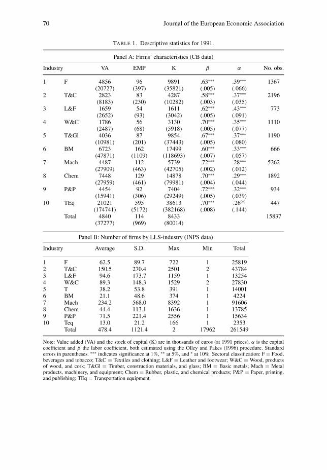
TABLE 1. Descriptive statistics for 1991.

Panel A: Firms’ characteristics (CB data)

Industry VA EMP K β α No. obs.

1 F 4856 96 9891 .63∗∗∗ .39∗∗∗ 1367(20727) (397) (35821) (.005) (.066)

2 T&C 2823 83 4287 .58∗∗∗ .37∗∗∗ 2196(8183) (230) (10282) (.003) (.035)

3 L&F 1659 54 1611 .62∗∗∗ .43∗∗∗ 773(2652) (93) (3042) (.005) (.091)

4 W&C 1786 56 3130 .70∗∗∗ .35∗∗∗ 1110(2487) (68) (5918) (.005) (.077)

5 T&Gl 4036 87 9854 .67∗∗∗ .37∗∗∗ 1190(10981) (201) (37443) (.005) (.080)

6 BM 6723 162 17499 .60∗∗∗ .33∗∗∗ 666(47871) (1109) (118693) (.007) (.057)

7 Mach 4487 112 5739 .72∗∗∗ .28∗∗∗ 5262(27909) (463) (42705) (.002) (.012)

8 Chem 7448 129 14878 .70∗∗∗ .29∗∗∗ 1892(27959) (461) (79981) (.004) (.044)

9 P&P 4454 92 7404 .72∗∗∗ .32∗∗∗ 934(15941) (306) (29249) (.005) (.039)

10 TEq 21021 595 38613 .70∗∗∗ .26(∗) 447(174741) (5172) (382168) (.008) (.144)

Total 4840 114 8433 15837(37277) (969) (80014)

Panel B: Number of firms by LLS-industry (INPS data)

Industry Average S.D. Max Min Total

1 F 62.5 89.7 722 1 258192 T&C 150.5 270.4 2501 2 437843 L&F 94.6 173.7 1159 1 132544 W&C 89.3 148.3 1529 2 278305 T 38.2 53.8 391 1 140016 BM 21.1 48.6 374 1 42247 Mach 234.2 568.0 8392 1 916068 Chem 44.4 113.1 1636 1 137859 P&P 71.5 221.4 2556 1 1563410 Teq 13.0 21.2 166 1 2353

Total 478.4 1121.4 2 17962 261549

Note: Value added (VA) and the stock of capital (K) are in thousands of euros (at 1991 prices). α is the capitalcoefficient and β the labor coefficient, both estimated using the Olley and Pakes (1996) procedure. Standarderrors in parentheses. ∗∗∗ indicates significance at 1%, ∗∗ at 5%, and ∗ at 10%. Sectoral classification: F = Food,beverages and tobacco; T&C = Textiles and clothing; L&F = Leather and footwear; W&C = Wood, productsof wood, and cork; T&Gl = Timber, construction materials, and glass; BM = Basic metals; Mach = Metalproducts, machinery, and equipment; Chem = Rubber, plastic, and chemical products; P&P = Paper, printing,and publishing; TEq = Transportation equipment.


the analysis to manufacturing.7 The capital stock is constructed using the permanentinventory method with sectoral deflators and depreciation rates, see Cingano andSchivardi (2004) for details.

We complement the CB data with another dataset on Italian industrial clusters, theLocal Labor Systems dataset. The territory of Italy has been divided by the NationalStatistical Institute (ISTAT) into 784 local labor systems (LLS) on the basis of working-day commuting areas.8 The idea behind the algorithm is to define self-contained labormarkets in terms of worker mobility. Since the Data Services gives the firm’s LLScode, we can match firms with the corresponding LLS. The number of manufacturingfirms in the LLS is obtained from the files of the Italian Social Security Administration(INPS) on the population of firms with at least one employee for the years 1986–1998.With respect to the CB, the information on firms is much less detailed: for example,output is not reported so that TFP cannot be computed. For our purposes, the databasecontains the number of employees, the sector, and the location of each firm, from whichvery precise measures of entrepreneurial density at the local and sectoral level can beconstructed. Panel B of Table 1 shows summary statistics on the average number offirms per LLS (as well as the total in the last column) for each of our 10 industries. Itis clear that there is considerable sectoral and geographical variation in the clusteringof industry: for the whole manufacturing, there are 478 firms per LLS with a standarddeviation almost three times the mean (1,121) and range of 1–17,962.

3.1 Measuring Entrepreneurial Incidence

The model has a series of predictions relating the share of potential entrepreneursthat actually become active (1 − �(z)) and the distribution of their ability x. Wenow construct the empirical counterpart of this share, which we name entrepreneurialincidence (EI). We have assumed that people are born in a LLS and decide to becomeentrepreneurs there or employees anywhere in the country. Therefore, the correctempirical counterpart of this theoretical construct is the number of entrepreneurs in alocation as a share of the “population at risk”, which is given by the total number ofindividuals currently alive that were born in such location, independently from theircurrent LLS of residence.

To get this measure we rely on the 1991 census which contains data on themunicipality where each individual alive in 1991 was born. We select all the individualsin the 1991 census aged 20–65 (our definition of working age) and aggregate themaccording to the LLS where they were born. This procedure only leaves out from

7. As will become clear in the next section, the sectoral classification balances the need for homogeneityof the production technology and that of a sufficient number of sectoral observations to properly estimateTFP.8. Even if defined using the same criteria (commuting ties), the concept of LLS differs from U.S. CoreBased Statistical Areas since there is no minimum population requirement. Hence, like the French zonesd’emploi, the Italian LLS entirely and continuously cover the national territory. The average land-areais 384 square kilometers, with a population density of 188 inhabitants per square kilometer. Populationranges from 3,000 in the smallest LLS to 3.3 million in the largest.


the population of potential entrepreneurs those who migrated abroad, for whom noinformation is available. We then divide the total number of firms active in a given LLS(the entrepreneurs) by the number of individuals born there of working age. This is ourmeasure of entrepreneurial incidence, EI. We use the 1991 measure of the populationat risk also for the other years in our sample (1986–1994).9

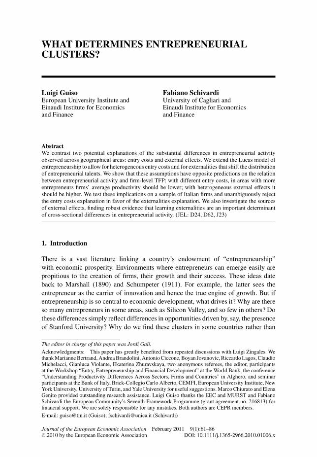
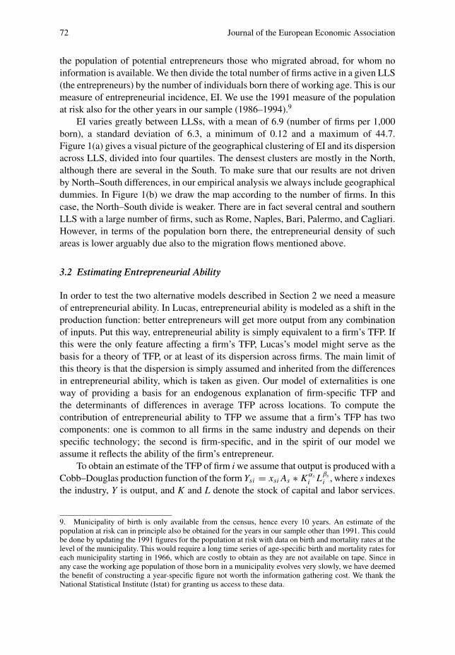
EI varies greatly between LLSs, with a mean of 6.9 (number of firms per 1,000born), a standard deviation of 6.3, a minimum of 0.12 and a maximum of 44.7.Figure 1(a) gives a visual picture of the geographical clustering of EI and its dispersionacross LLS, divided into four quartiles. The densest clusters are mostly in the North,although there are several in the South. To make sure that our results are not drivenby North–South differences, in our empirical analysis we always include geographicaldummies. In Figure 1(b) we draw the map according to the number of firms. In thiscase, the North–South divide is weaker. There are in fact several central and southernLLS with a large number of firms, such as Rome, Naples, Bari, Palermo, and Cagliari.However, in terms of the population born there, the entrepreneurial density of suchareas is lower arguably due also to the migration flows mentioned above.

3.2 Estimating Entrepreneurial Ability

In order to test the two alternative models described in Section 2 we need a measureof entrepreneurial ability. In Lucas, entrepreneurial ability is modeled as a shift in theproduction function: better entrepreneurs will get more output from any combinationof inputs. Put this way, entrepreneurial ability is simply equivalent to a firm’s TFP. Ifthis were the only feature affecting a firm’s TFP, Lucas’s model might serve as thebasis for a theory of TFP, or at least of its dispersion across firms. The main limit ofthis theory is that the dispersion is simply assumed and inherited from the differencesin entrepreneurial ability, which is taken as given. Our model of externalities is oneway of providing a basis for an endogenous explanation of firm-specific TFP andthe determinants of differences in average TFP across locations. To compute thecontribution of entrepreneurial ability to TFP we assume that a firm’s TFP has twocomponents: one is common to all firms in the same industry and depends on theirspecific technology; the second is firm-specific, and in the spirit of our model weassume it reflects the ability of the firm’s entrepreneur.

To obtain an estimate of the TFP of firm i we assume that output is produced with aCobb–Douglas production function of the form Ysi = xsi As ∗ K αs

i Lβsi , where s indexes

the industry, Y is output, and K and L denote the stock of capital and labor services.

9. Municipality of birth is only available from the census, hence every 10 years. An estimate of thepopulation at risk can in principle also be obtained for the years in our sample other than 1991. This couldbe done by updating the 1991 figures for the population at risk with data on birth and mortality rates at thelevel of the municipality. This would require a long time series of age-specific birth and mortality rates foreach municipality starting in 1966, which are costly to obtain as they are not available on tape. Since inany case the working age population of those born in a municipality evolves very slowly, we have deemedthe benefit of constructing a year-specific figure not worth the information gathering cost. We thank theNational Statistical Institute (Istat) for granting us access to these data.


FIGURE 1. EI and number of firms in the Italian LLSs. (a) Distribution of EI (no. of firms per 1000born), dividing the LLSs into four percentiles; (b) distribution of the number of firms, also split into fourpercentiles.


TFP is given by TFPsi = xsi As , and is the product of the sectoral component, A, andthe firm-specific component, x. The latter is our measure of entrepreneurial ability. Toobtain an estimate of TFP we need to compute values for αs and βs . To obtain estimatesof the production function parameters that are robust to the endogeneity of some of theinputs (capital accumulation and labor demand may respond to unobserved productivityshocks) and the selection induced by exit (with some irreversibility, leaving the industryis more likely for firms with a lower capital stock when a bad productivity shock occurs)we use the multi-step estimation algorithm proposed by Olley and Pakes (1996), whichaccounts for both problems, allowing for consistent and unconstrained estimation ofαs and βs .10 To assess the reliability of the estimates, we have also calculated thecoefficients using Solow’s assumptions, finding similar results.

Table 1, columns (4) and (5), reports the estimated values of αs and βs . Productionfunction estimates of (αs + βs) lie in the range 0.93–1.05. The model assumesdecreasing returns to scale to avoid a degenerate equilibrium in which there existsonly one firm supplying the whole market. Given that the capital coefficient isestimated using a semi-parametric procedure, we obtained its standard errors througha bootstrapping exercise based on 150 replications. As in Olley and Pakes (1996),standard errors are relatively large11 and, given that the estimates of (αs + βs) arealways somewhere around 1, the empirical model has no power to discriminate betweendifferent degrees of returns to scale. Formally, the null hypothesis (αs + βs) < 1 isnever rejected in a one-sided test even at the 10 per cent confidence level.12

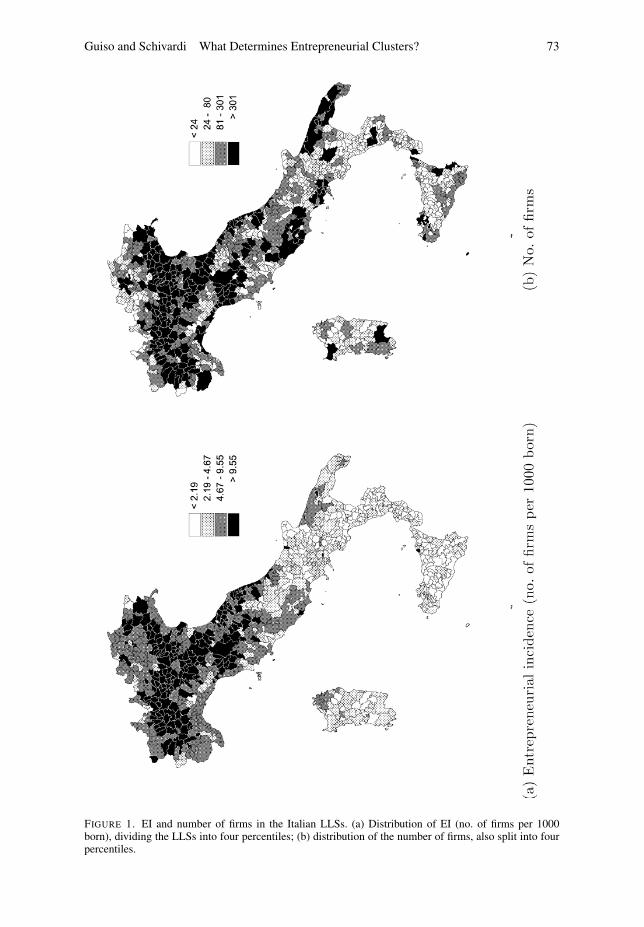
Table 2 gives a first appreciation of the relation between EI and ability distribution(as well as other characteristics of the LLS), relative to the reference year 1991. Weremove the industry-level component of our estimate of x with a first-stage regressionof estimated TFP on a set of industry dummies. To account for possible outliers we dropobservations in the first and last percentile of the ability distribution by year. The samplemean of entrepreneurial ability is 2.35 but there is considerable dispersion, as the highvalue of the standard deviation (0.5) implies. When the sample is split according to EI,entrepreneurial ability is substantially higher where EI is above median than where itis below median (2.38 compared to 2.16), which is inconsistent with the start-up costhypothesis but not with heterogeneity in local externalities. The table also shows theshare of firms with TFP below the 25th and above the 75th percentile both for the totalsample and the two sub-samples of high-density and low-density areas. Contrary to thestart-up cost model, there is a larger frequency mass to the left of the lower thresholdin places with lower EI (40% in the low-density group compared with 22% among

10. To summarize, the procedure deals with endogeneity by approximating the unobserved productivityshocks with a non-parametric function of observable variables and for selection by introducing a Heckman-type correction term.11. Pakes and Olley (1995) discuss the asymptotic properties of the estimator, suggesting that thebootstrapping procedure might overestimate the true standard deviation of the capital coefficient, partiallyexplaining why its values are higher than those for labor.12. Indeed, returns to scale might be initially increasing, due for example to fixed production costs, sothat the “span of control” only kicks in for larger levels of operation. In fact, some small, yet growing firmsmight still be on the increasing part of the production function but, due to convex costs of adjusting thescale of operation, might not immediately exploit the full advantages of scale.


TABLE 2. Ability and other characteristics by Entrepreneurial Incidence.

Variable Mean S.D. Mean S.D. Mean S.D.

Total sample High EI LLS Low EI LLS

Ability 2.35 0.50 2.38 0.48 2.16 0.58I[Ability<25%] 0.25 0.43 0.22 0.42 0.40 0.49I[Ability>75%] 0.25 0.43 0.26 0.44 0.18 0.39No. firms 5.18 1.41 5.94 1.10 4.42 1.28Avg. firm size 2.28 0.51 2.48 0.33 2.08 0.57No. workers 7.46 1.70 8.42 1.22 6.49 1.57Intermediate inputs/VA 0.86 0.65 0.84 0.50 0.89 0.78

Ability, No. firms, No. workers and Intermediate inputs/VA are in log. High EI LLS are defined as EI above themedian value by LLS. Ability is the log of TFP. I[Ability<25%] is 1 if the ability is below the 25th percentile of theability distribution and zero otherwise; correspondingly for I[Ability<75%]. Ability and intermediate inputs overvalue added are from the CB sample; the number of firms, of workers and average firm size are computed fromthe INPS dataset (the population).

Density

Log of entrepreneurial ability

High EI Low EI

0 1 2 3 4

0

.5

1

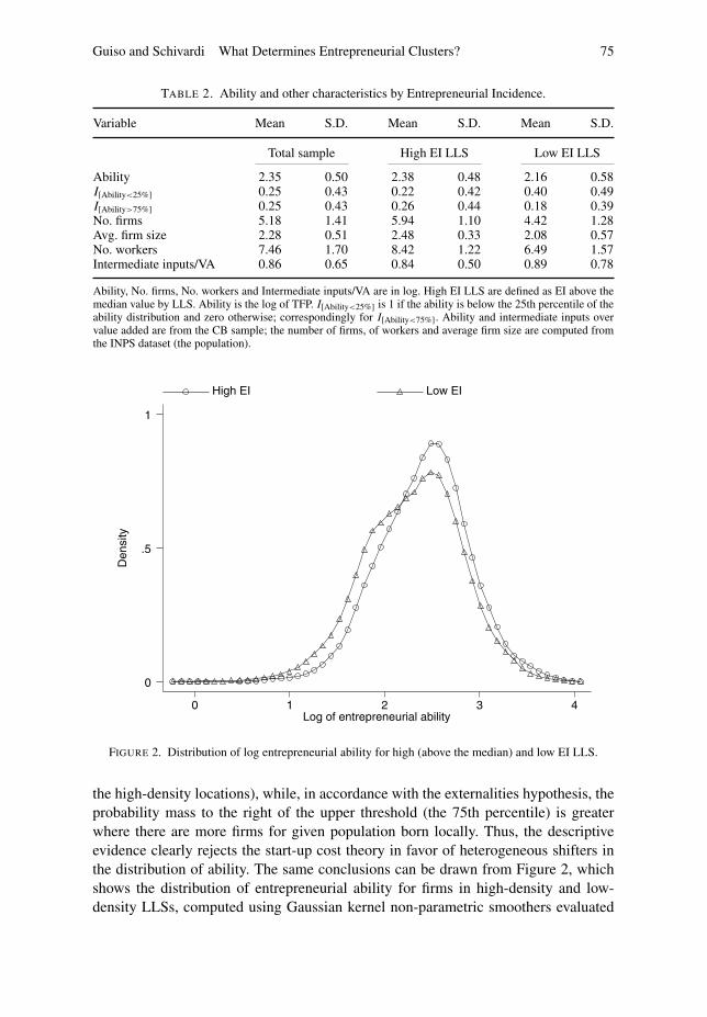
FIGURE 2. Distribution of log entrepreneurial ability for high (above the median) and low EI LLS.

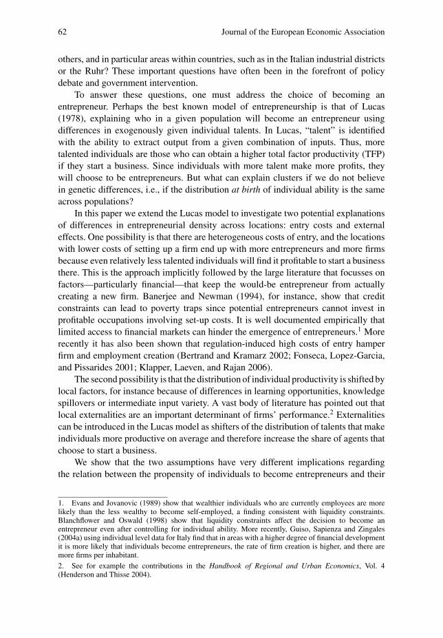
the high-density locations), while, in accordance with the externalities hypothesis, theprobability mass to the right of the upper threshold (the 75th percentile) is greaterwhere there are more firms for given population born locally. Thus, the descriptiveevidence clearly rejects the start-up cost theory in favor of heterogeneous shifters inthe distribution of ability. The same conclusions can be drawn from Figure 2, whichshows the distribution of entrepreneurial ability for firms in high-density and low-density LLSs, computed using Gaussian kernel non-parametric smoothers evaluated


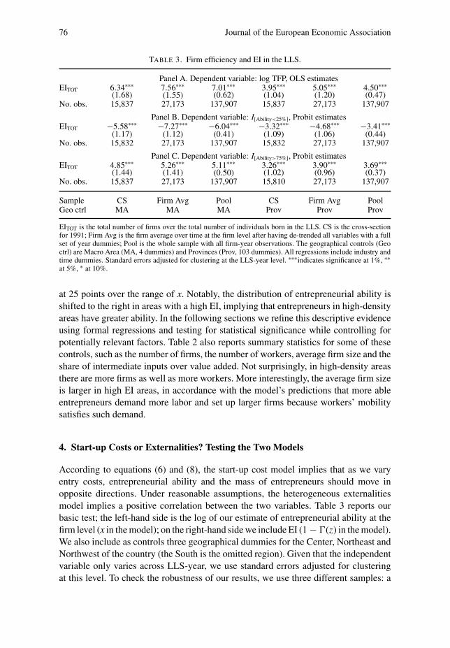
TABLE 3. Firm efficiency and EI in the LLS.

Panel A. Dependent variable: log TFP, OLS estimatesEITOT 6.34∗∗∗

(1.68)7.56∗∗∗(1.55)

7.01∗∗∗(0.62)

3.95∗∗∗(1.04)

5.05∗∗∗(1.20)

4.50∗∗∗(0.47)

No. obs. 15,837 27,173 137,907 15,837 27,173 137,907

Panel B. Dependent variable: I[Ability<25%], Probit estimatesEITOT −5.58∗∗∗

(1.17)−7.27∗∗∗

(1.12)−6.04∗∗∗

(0.41)−3.32∗∗∗

(1.09)−4.68∗∗∗

(1.06)−3.41∗∗∗

(0.44)No. obs. 15,832 27,173 137,907 15,832 27,173 137,907

Panel C. Dependent variable: I[Ability>75%], Probit estimatesEITOT 4.85∗∗∗

(1.44)5.26∗∗∗(1.41)

5.11∗∗∗(0.50)

3.26∗∗∗(1.02)

3.90∗∗∗(0.96)

3.69∗∗∗(0.37)

No. obs. 15,837 27,173 137,907 15,810 27,173 137,907

Sample CS Firm Avg Pool CS Firm Avg PoolGeo ctrl MA MA MA Prov Prov Prov

EITOT is the total number of firms over the total number of individuals born in the LLS. CS is the cross-sectionfor 1991; Firm Avg is the firm average over time at the firm level after having de-trended all variables with a fullset of year dummies; Pool is the whole sample with all firm-year observations. The geographical controls (Geoctrl) are Macro Area (MA, 4 dummies) and Provinces (Prov, 103 dummies). All regressions include industry andtime dummies. Standard errors adjusted for clustering at the LLS-year level. ∗∗∗indicates significance at 1%, ∗∗at 5%, ∗ at 10%.

at 25 points over the range of x. Notably, the distribution of entrepreneurial ability isshifted to the right in areas with a high EI, implying that entrepreneurs in high-densityareas have greater ability. In the following sections we refine this descriptive evidenceusing formal regressions and testing for statistical significance while controlling forpotentially relevant factors. Table 2 also reports summary statistics for some of thesecontrols, such as the number of firms, the number of workers, average firm size and theshare of intermediate inputs over value added. Not surprisingly, in high-density areasthere are more firms as well as more workers. More interestingly, the average firm sizeis larger in high EI areas, in accordance with the model’s predictions that more ableentrepreneurs demand more labor and set up larger firms because workers’ mobilitysatisfies such demand.

4. Start-up Costs or Externalities? Testing the Two Models

According to equations (6) and (8), the start-up cost model implies that as we varyentry costs, entrepreneurial ability and the mass of entrepreneurs should move inopposite directions. Under reasonable assumptions, the heterogeneous externalitiesmodel implies a positive correlation between the two variables. Table 3 reports ourbasic test; the left-hand side is the log of our estimate of entrepreneurial ability at thefirm level (x in the model); on the right-hand side we include EI (1 − �(z) in the model).We also include as controls three geographical dummies for the Center, Northeast andNorthwest of the country (the South is the omitted region). Given that the independentvariable only varies across LLS-year, we use standard errors adjusted for clusteringat this level. To check the robustness of our results, we use three different samples: a


single cross section in 1991, which is the Census year when the locally born populationis counted; the de-trended firm average over the entire period;13 and the full 1986–1994panel with year dummies. The first column shows the estimates using the 1991 cross-section; the correlation between EI and TFP is positive and statistically significant at1%; to give a sense of its magnitude, moving from the 25th to the 75th percentile ofthe EI distribution results in an increase in TFP of 5%. Using firm averages and pooleddata (columns (2) and (3)), the estimate increases slightly. This clearly contradicts thestart–up cost model of business cluster formation already questioned by the previousdescriptive evidence. This result is very robust across specifications.

One possible objection to these regressions is that macro areas might differalong several dimensions that affect both entry costs and firm performance. Forexample, Guiso, Sapienza and Zingales (2004b) have shown that the endowmentof social capital, which might conceivably reduce entry costs and also increaseaverage productivity, varies greatly across Italian provinces. To control for unobservedfactors at the local level, we run the regressions including province dummies; thisis a very fine geographical control as Italy is partitioned into 103 provinces, so thateach is comprised on average by less than eight LLSs. This level of controls shouldaccount for most correlated geographical factors, including the social capital indicatorsdeveloped in the literature, which typically vary by province. The estimated coefficientof entrepreneurial density is lower (3.95 compared to 6.34 in the cross sectionalsample), an indication of possible spatially correlated effects, but still positive andstatistically significant at 1% in all specifications. The effect of a shift from the 25thto the 75th percentile of the EI distribution is an increase in TFP of 3.3%.

The second panel of Table 3 sharpens the evidence on the validity of the start-upcost theory by looking at the relationship between the number of firms in a cluster andthe share of them with ability below a lower bound or above an upper one. Accordingto this model, there should be a positive (negative) correlation between the numberof firms and the frequency of firms with ability below (above) a certain bound. Theintuition is that as the start-up cost declines and the number of firms increases, the newentrants are of lower quality, so there is a larger (smaller) mass of entrepreneurs withability below (above) any given threshold. To test this implication we set the lowerbound at the 25th (and the upper at the 75th) percentile of the empirical distribution ofability and construct an indicator that is equal to 1 if the firm’s specific ability is below(above) the threshold. We then run a probit estimate on the entrepreneurial share and thegeographical controls. The first three columns of Table 3 show the results for the sharebelow the 25th percentile for the three samples, using macro areas as geographicalcontrols. They reveal a negative correlation with highly significant coefficients. Thispattern is confirmed when provinces are used as geographical controls (last threecolumns). The last panel shows the share of firms above the 75th percentile, finding apositive coefficient of EI, highly significant in all specifications. Taken together, these

13. According to Bertrand, Duflo and Mullainathan (2004), the serial correlation in the independentvariable can make inference problematic. As a simple solution, they propose to run estimates on thecollapsed data ignoring the time series variation. We, therefore, first run a regression of firm-level TFP ona set of year dummies to clean for cyclical effects and then take the firm-level average.


findings suggest that a larger share of firms is associated with a shift to the right in thedistribution of entrepreneurial talent. Thus, the two main implications of the start-upcost model are strongly rejected by the data. On the other hand, they are consistentwith externalities, which (under mild conditions) not only predict a positive correlationbetween ability and the share of entrepreneurs, but also a negative correlation betweenthe share of firms with ability below a lower bound and EI (and vice versa for the righttail).

In a series of unreported exercises we have performed additional robustness checks.First, our analysis is cast in a steady-state setting, so that we do not consider directlyentry and exit. One could argue that specific patterns of entry and exit might beresponsible for the correlation between the number of firms and average productivitythat we find. To dispel this possibility, we have repeated the regressions including theentry and exit rates at the LLS level computed from the archives of the Italian SocialSecurity Administration (INPS). We find that the estimates of EI are unaffected, whileno clear cut relation emerges between TFP and exit and entry rates. Another potentialconcern is firm size. Traditionally, industrial districts are characterized by a networkof small, efficient and connected firms (Guiso and Schivardi 2007). It could be thatthe correlation we find reflects the fact that small firms are more efficient and thatEI is higher where firms are smaller (typically in industrial districts). Table 2 alreadysuggests that this is not the case, as denser LLS have larger, not smaller average firmsize. To further exclude this possibility, we have added average firm size in the LLS,finding again no significant change in the coefficient of EI and, if anything, a positivecorrelation between average firm size and TFP. This is also true at the individual firmlevel: we find that TFP is positively correlated with various measures of size, suchas total assets and sales. The evidence in Table 3 is therefore unequivocal: it stronglyrejects the theories of cluster formation based only on differences in entry and start-upcosts, such as differences in the fixed costs or bureaucratic steps required to organizea firm. It lends support to models that emphasize differences in the distribution ofentrepreneurial abilities, possibly due to local externalities.

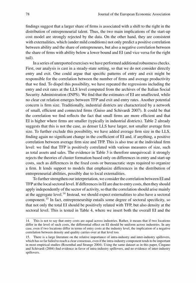
To further strengthen our interpretation, we consider the correlation between EI andTFP at the local sectoral level. If differences in EI are due to entry costs, then they shouldapply independently of the sector of activity, so that the correlation should arise mainlyat the aggregate level.14 Instead, we should expect externalities to also have a sectoralcomponent.15 In fact, entrepreneurship entails some degree of sectoral specificity, sothat not only the total EI should be positively related with TFP, but also density at thesectoral level. This is tested in Table 4, where we insert both the overall EI and the

14. This is not to say that entry costs are equal across industries. Rather, it means that if two locationsdiffer in the level of such costs, the differential effect on EI should be uniform across industries. In anycase, even if two locations differ in terms of entry costs at the industry level, the implication of a negativecorrelation between density and quality carries over at that level too.15. There is a large literature on the relative importance of intra-industry and inter-industry spillovers,which has so far failed to reach a clear consensus, even if the intra-industry component tends to be importantin most empirical studies (Rosenthal and Strange 2004). Using the same dataset as in this paper, Cinganoand Schivardi (2004) find evidence in favor of intra-industry spillovers, and no evidence of inter-industryspillovers.


TABLE 4. Firm efficiency and EI in the LLS-sector.

Panel A. Dependent variable: log TFP, OLS estimatesEITOT 4.48∗∗∗

(1.13)5.56∗∗∗(1.04)

4.78∗∗∗(.40)

2.00∗(1.09)

2.37∗∗(1.06)

2.02∗∗∗(.41)

EISECT 3.55(2.47)

3.51∗(2.05)

4.03∗∗∗(.90)

3.27∗∗(1.40)

4.15∗∗∗(1.19)

4.04∗∗∗(.63)

No. obs. 15,837 27,173 137,907 15,837 27,173 137,907

Panel B. Dependent variable: I[Ability<25%], Probit estimatesEITOT −4.77∗∗∗

(1.12)−6.90∗∗∗

(1.01)−5.70∗∗∗

(.40)−1.93(1.24)

−3.20∗∗∗(1.10)

−2.56∗∗∗(.47)

EISECT −1.57(1.84)

.66(1.73)

−.62(.68)

−2.39∗(1.38)

−2.36∗(1.23)

−1.40∗∗∗(.56)

No. obs. 15,837 27,173 137,907 15,832 27,173 137,907

Panel C. Dependent variable: I[Ability>75%], Probit estimatesEITOT 2.60∗∗

(1.13)2.75∗∗∗(1.00)

2.64∗∗∗(.39)

1.04(1.25)

1.09(1.12)

1.09∗∗(.43)

EISECT 4.19∗∗(1.91)

4.30∗∗∗(1.75)

4.37∗∗∗(.61)

3.61∗∗∗(1.32)

4.24∗∗∗(1.14)

4.14∗∗∗(.46)

No. obs. 15,837 27,173 137,907 15,810 27,173 137,907

Sample CS Firm Avg Pool CS Firm Avg PoolGeo controls MA MA MA Prov Prov Prov

EITOT is the total number of firms over the total number of individuals born in the LLS, EISECT is the total numberof firms in the LLS-sector over the total number of individuals born in the LLS. CS is the cross-section for 1991;Firm Avg is the firm average over time at the firm level after having de-trended all variables with a full set ofyear dummies; Pool is the whole sample with all firm-year observations. The geographical controls are MacroArea (MA, 4 dummies) and Provinces (Prov, 103 dummies). All regressions include industry and time dummies.Standard errors adjusted for clustering at the LLS-year level. ∗∗∗indicates significance at 1%, ∗∗ at 5%, ∗ at 10%.

EI at the sectoral level, i.e., calculated using the number of firms in an LLS-industryover the working age population born in the LLS. The first panel shows the resultsfor the correlation between ability and the two indexes of entrepreneurial density. Wefind that both indexes are positively correlated with productivity. In particular, theoverall EI has a larger and more significant coefficient in the specification with themacro area geographical controls, while the reverse occurs with provincial controls.This arguably reflects the fact that the overall EI is more strongly correlated with localattributes that are not fully captured by macro area dummies but are picked up by thefiner geographical controls, while the sectoral EI reflects more direct external effects.

The second and third panels report the regressions for the probability that a firm’sTFP is below the 25th percentile of the distribution (Panel B) and above the 75thpercentile (Panel C). The pattern is very similar to that found in Panel A, with bothindicators being significant in most specifications. All in all, the evidence points to apositive correlation between sectoral EI and productivity. This is consistent with theexternalities hypothesis and at odds with the idea that some locations have more firmsonly because of lower start-up costs.

5. Which Externalities?

Up to now, we have used the model to obtain equilibrium correlations between EIand ability, without any causal interpretation. Empirically, we showed that the TFP


distribution and EI display a positive correlation. We now take a further step andinvestigate the underlying factors that can explain the rightward shift in the TFPdistribution. In practice, by log linearizing (12), we can immediately verify that thisamounts to identifying some measurable factors that shift the entrepreneurs’ abilitydistribution (the variable λ in the model) and to running a regression of (log) abilityon the (log) indicator of λ. The logical candidate to explain productivity differencesaccording to density is local externalities. In this section, therefore, we contrast differentsources of externalities to look for more direct evidence that can sort out their nature.

There is a large theoretical literature on agglomeration economies (see Durantonand Puga (2004) for a recent survey). This literature has maintained the originalMarshallian idea (Marshall 1890) that the spatial concentration of production can bebeneficial for three reasons. First, concentration fosters the circulation of ideas andthe possibility of learning from other agents. Second, a large concentration of workersin the same industry can have beneficial effects both in terms of the specializationthat each worker can achieve and the quality of worker/job matches. Third, industrialclusters offer a wide variety of intermediate inputs, with potentially beneficial effectson productivity.16 The empirical literature on the extent and scope of agglomerationeconomies suggests that localization economies are important. However, a consensushas not yet emerged on the relative merits of the different sources and investigationis continuing (see Rosenthal and Strange (2004) for an exhaustive assessment of thestate of the empirical debate).

We distinguish among these different effects by proposing a proxy for eachpotential externality. To proxy for learning externalities we use the number of firmsoperating in a given industry and in a given location. According to Guiso and Schivardi(2007), this is the reference group within which information flows are most intense.If learning entrepreneurial abilities is not, as we think, a routine activity, then anobvious feature facilitating it is the number of firms in a given location. If learningtakes place mainly on the job and on the site, a larger number of firms offers more (andbetter) opportunities to acquire entrepreneurial abilities, since a potential entrepreneurcan compare different working practices and business ideas, possibly by working indifferent firms.17 Moreover, the process of knowledge acquisition continues even after

16. Marshall (1890) wrote: “When an industry has thus chosen a locality for itself, it is likely to stay therelong: so great are the advantages which people following the same skilled trade get from neighborhood toone another. The mysteries of trade become no mysteries; but are as in the air, and children learn manyof them unconsciously. . . . Employers are apt to resort to any place where they are likely to find a goodchoice of workers with the special skill which they require. . . . The advantages of variety of employmentare combined with those of localized industries in some of our manufacturing towns, and this is a chiefcause of their continued economic growth.”17. According to Saxenian (1994), the mobility of workers across firms and their acquired capacity tostart up new firms was one of the main reasons behind the success of Silicon Valley during the technologyboom. This would also be consistent with the model and the empirical evidence of Lazear (2005), accordingto which the probability of becoming an entrepreneur is positively related to the number of tasks a workeris previously exposed to, because the entrepreneur needs to be able to understand and coordinate differentactivities. Again, more firms could offer better opportunities of learning the complex set of skills requiredto manage a firm.


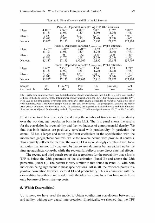
TABLE 5. Firm efficiency and externalities.

Dependent variable: log TFP, OLS estimatesNo. firms .051∗∗∗

(.009).046∗∗∗(.009)

.048∗∗∗(.003)

.031∗∗∗(.007)

.024∗∗∗(.006)

.028∗∗∗(.003)

.0115(.009)

.018∗∗∗(.008)

.019∗∗∗(.003)

Int.Inputs/VA .020(.013)

.063∗∗∗(.011)

.028∗∗∗(.004)

.009(.011)

.052∗∗∗(.010)

.015∗∗∗(.004)

.007(.011)

.046∗∗∗(.010)

.006(.004)

Labor −.007(.005)

−.001(.005)

−.005∗∗(.002)

−.001(.004)

.004(.004)

.001(.002)

.005(.005)

.004(.004)

.002∗∗(.002)

No obs. 15,837 27,173 137,907 15,837 27,173 137,907 15,837 27,173 137,907

Sample CS Firm Avg Pool CS Firm Avg Pool CS Firm Avg PoolGeo controls MA MA MA Prov Prov Prov LLS LLS LLS

No. firms, Int.Inputs/VA, and Labor are in logs and computed at the LLS-industry level. CS is the cross-sectionfor 1991; Firm Avg is the firm average over time at the firm level after having de-trended all variables with a fullset of year dummies; Pool is the whole sample with all firm-year observations. The geographical controls areMacro Area (MA), Provinces (Prov) and Local Labor Systems (LLS). All regressions include industry and timedummies. Standard errors adjusted for clustering at the LLS-year level. ∗∗∗indicates significance at 1%, ∗∗ at 5%,∗ at 10%.

the business is started, because knowledge spillovers on alternative technologies ornew markets keep accruing in regions with a large population of firms. According tothis interpretation, what matters for learning is the number of “data points” available, sothat the relevant measure of spillovers is the absolute number of firms. This is differentfrom the approach of the previous section, where we characterized the equilibriumcorrelation between the share of local born population becoming entrepreneurs andtheir ability distribution. The availability of intermediate inputs—the second reasonwhy spatial concentration can raise firms’ productivity—is easily measured by theratio of intermediate inputs to value added at the local sectoral level. In fact, if greaterconcentration leads to higher productivity through more reliance on intermediateinputs,18 we should find that TFP is positively related to this indicator. The thirdreason, the labor market pooling effect, is measured by the number of workersoperating in a given LLS-sector. Summary statistics for these variables are reported inTable 2.

5.1 Main Results

In Table 5 we regress firm-level TFP on the number of firms, the share of intermediateinputs over value added and the number of workers, with all the variables computedat the LLS-industry level (all variables are in logs).19 To save on space, in all theremaining tables we omit the probit results, which fully confirm those of the OLS.20

18. Using U.S. data, Holmes (1999) finds that sectoral concentration at the local level is positively relatedto intermediate input intensity, although the effect is rather modest.19. While the number of firms and the number of workers can be computed from the INPS dataset,covering the respective populations, we have information on intermediate inputs and value added only forthe CB sample, which is used to compute the measure of intermediate input intensity.20. The interested reader can find them in a previous version of this paper (Guiso and Schivardi 2005).


With four spatial controls, we find that the number of firms has a positive and significantcoefficient in all specifications, with a value of around 0.05. The share of intermediateinputs is not significantly different from zero in the cross-sections, but is significantwhen using averaged data and in the pooled data. Thus there are indications thatthe availability of intermediate inputs might also foster local productivity, though theevidence is less clear-cut than for the number of firms. The number of workers is neversignificant, save in one case. The exception is found in the pooled data with four spatialcontrols, and its negative coefficient is at odds with the idea that local externalitiesare attributable to labor market pooling effects. To give a sense of the magnitude ofthese effects, using the pooled estimate of column (3) we calculate that increasing thenumber of firms by one standard deviation would bring about an increase in firms’productivity of about 9%, which is quite large; doing the same with intermediate inputintensity would increase TFP by a more modest 1.2%. The next three columns ofTable 5 repeat the exercise with 103 spatial controls (the province dummies). Theestimates for the number of firms and the intermediate inputs become somewhatsmaller, but remain highly significant. The number of workers has no effect in anyspecification.

All in all, we conclude that the evidence supports both learning externalities andintermediate input variety, with the former playing a more prominent role. Controllingfor these sources, no evidence of labor market pooling emerges.

5.2 Robustness and Further Implications

Having established that the number of firms is strongly correlated with firm-level TFP,we further investigate if we can correctly interpret this correlation as evidence in favorof learning externalities, as suggested above.

The OLS correlations face the endogeneity problem that plagues the empiricalanalysis of density and productivity. There could in fact be unobserved local factorscausing both and not accounted for by our geographical controls, as even the finerones (the province dummies) refer to wider areas than the Local Labor System. Forexample, politicians might care about places with a high production density and providebusiness-oriented public goods, such as infrastructure, which raise productivity. Whilethe province dummies absorb some of these effects, the transfers could take placeat an even finer geographical level, leaving the regression residual correlated withthe number of firms. We address this issue in two ways. First, since our regressorsvary with the LLS and the industry, we can exploit the cross-industry variation whileinserting geographical controls at the LLS level. In the last three columns of Table 5 wereport the same regressions as in the previous table, adding a dummy for each LLS. Wefind results that are similar to those of the previous columns with province dummies,losing significance only in the case of the cross-section sample. Indeed, in a similarvein, Henderson (2003) finds a positive and robust correlation between the number of


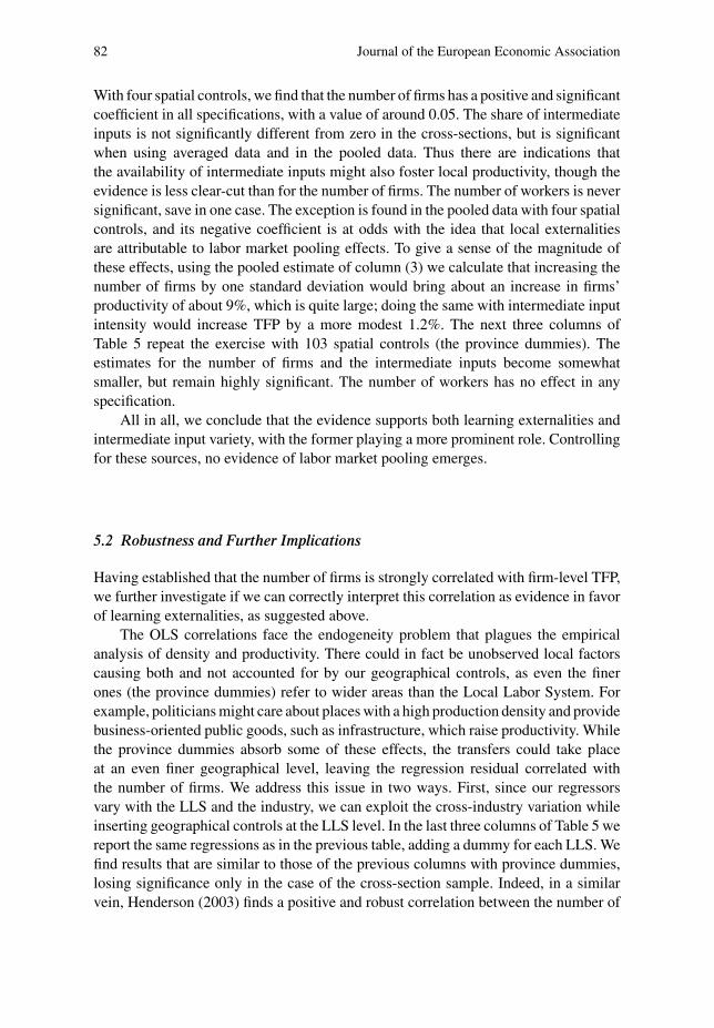
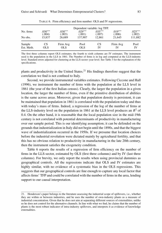
TABLE 6. Firm efficiency and firm number: OLS and IV regressions.

Dependent variable: log TFP.No. firms .030∗∗∗

(.004).030∗∗∗(.003)

.029∗∗∗(.001)

.035∗∗∗(.007)

.019∗∗∗(.006)

.025∗∗∗(.002)

No obs. 15,837 26,689 137,907 12,861 21,645 111,882

Sample CS Firm Avg Pool CS Firm Avg PoolEst. Meth. OLS OLS OLS IV IV IV

The first three columns report OLS estimates; the fourth to sixth columns are IV estimates. The instrumentused is the population in the LLS in 1861. The Number of firms is in log and computed at the LLS-industrylevel. Standard errors adjusted for clustering at the LLS-sector–year level. See Table 3 for the explanation of thespecifications.

plants and productivity in the United States.21 His findings therefore suggest that thecorrelation we find is not confined to Italy.

Second, we provide instrumental variables estimates. Following Ciccone and Hall(1996), we instrument the number of firms with the population at the LLS level in1861 (the year of the first Italian census). Clearly, the larger the population in a givenlocation, the larger the number of firms, even if the primitive distribution of abilitiesis the same across areas. Moreover, given that population density is persistent, it canbe maintained that population in 1861 is correlated with the population today and thuswith today’s mass of firms. Indeed, a regression of the log of the number of firms atthe LLS-industry level on the population in 1861 at the LLS level produces an R2 of0.4. On the other hand, it is reasonable that the local population size in the mid-19thcentury is not correlated with potential determinants of productivity in manufacturingover our sample period. This is our identifying assumption; it can be defended on thegrounds that industrialization in Italy did not begin until the 1890s, and that the biggestwave of industrialization occurred in the 1950s. If we presume that location choicesbefore the industrial revolution were dictated mainly by agricultural fertility, and thatthis has no obvious relation to productivity in manufacturing in the late 20th century,then the instrument satisfies the exogeneity condition.

Table 6 reports the results of a regression of firm efficiency on the number offirms in the LLS-sector, estimated by OLS (first three columns) and by IV (last threecolumns). For brevity, we only report the results when using provincial dummies asgeographical controls. All the regressions indicate that OLS and IV estimates arehighly similar, with no evidence of a systematic bias in the OLS regressions. Thissuggests that our geographical controls are fine enough to capture any local factor thataffects firms’ TFP and could be correlated with the number of firms in the area, lendingsupport to our causal interpretation.

21. Henderson’s paper belongs to the literature assessing the industrial scope of spillovers, i.e., whetherthey are within or between industries, and he uses the number of own-industry plants as a measure ofindustrial concentration. Given that he does not aim at separating different sources of externalities, unlikeus he does not control for the alternative channels. In line with what we find, he claims that the number ofplants is the most robust indicator of intra-industry spillovers, and interprets it as evidence of knowledgeexternalities.


We have also performed robustness checks along the industry dimension. First, thetwo-digit classification we use might be too coarse and mix industries with differentcharacteristics. While a more refined analysis is difficult because of limited samplesize, particularly in the estimation of the production function coefficients, we canincrease the number of industry controls in the baseline regression. We have run thebasic regression on the pooled data including 296 dummies at the four-digit level,finding no substantial difference in the estimates. A second problem is that we imposethe same coefficient for the number of firms across different industries. While assessinglearning opportunities at the industry level is beyond the scope of this paper, we haverun a separate regression for each industry. In all industries we find that the numberof firms has a positive and significant effect on TFP, with coefficients ranging froma low of 0.017 for basic metal to a high of 0.067 for leather and footwear. As a finalcheck, we have added average firm size among the regressors, to insure that we arenot simply capturing a higher efficiency of small firms. As in the case of EI, we findthat such inclusion does not change the results, and that, if anything, average size ispositively correlated with TFP.

6. Conclusions

This paper has compared two alternative theoretical models of cluster formation,one based on the cost of setting up a business and the other on local externalities.These models carry opposite implications on the sign of the correlation betweenentrepreneurial ability and entrepreneurial incidence, defined as the number of firmsover the number of individuals born in a given location. This relation is negative ifgeographical agglomeration of firms is due predominantly to start-up costs and positiveif agglomeration is driven predominantly by differences in externalities. The modelsalso have clear-cut implications for the relation between entrepreneurial incidence andthe frequency mass at the two tails of the ability distribution. We have confrontedthese theoretical predictions with data on a large sample of Italian manufacturing firmscoupled with information on the geographical clusters to which the firms belong. Wehave found overwhelmingly that a model with only start-up costs is rejected and theexternalities hypothesis is strongly supported.

When exploring the sources of externalities, we have found supporting evidencefor intermediate input variety and especially for learning spillovers. We have indeedshown that the data agree with specific predictions of knowledge spillovers models.In future work we plan to investigate the modes through which these spillovers takeplace, focussing in particular on the possibility that in some locations it might be easierto accumulate entrepreneurial skills.

Supporting Information

Additional Supporting Information may be found in the online version of this article:

Appendix S1. Experimental datasets (Zip archive).


Please note: Blackwell Publishing are not responsible for the content or functionalityof any supporting materials supplied by the authors. Any queries (other than missingmaterial) should be directed to the corresponding author for the article.

References

Banerjee, Abhijit V., and Andrew F. Newman (1994). “Poverty, Incentives and Development.”American Economic Review Papers and Proceedings, 84, 211–215.

Barlow, Richard, and Frank Proschan (1975). Statistical Theory of Reliability and Life Testing. Holt,Rinehart and Winston, New York.

Bertrand, Marianne, Ester Duflo, and Sendhil Mullainathan (2004). “How Much Should we TrustDifferences-in-differences Estimates?” Quarterly Journal of Economics, 119, 249–275.

Bertrand, Marianne, and Francis Kramarz (2002). “Does Entry Regulation Hinder Job Creation?Evidence from the French Retail Industry.” Quarterly Journal of Economics, 117, 1369–1413.

Blanchflower, David G., and Andrew Oswald (1998). “What Makes an Entrepreneur?” Journal ofLabor Economics, 16, 26–60.

Ciccone, Antonio, and Robert E. Hall (1996). “Productivity and the Density of Economic Activity.”American Economic Review, 86, 54–70.

Cingano, Federico, and Fabiano Schivardi (2004), “Identifying the Sources of Local ProductivityGrowth.” Journal of the European Economic Association, 2, 720–742.

Duranton, Gilles, and Diego Puga (2004). Micro-foundations of Urban Agglomeration Economies.In Handbook of Regional and Urban Economics, Vol. 4, edited by V. Henderson and J. Thisse.North-Holland, Amsterdam.

Evans, David S., and Bojan Jovanovic (1989). “An Estimated Model of Entrepreneurial ChoiceUnder Liquidity Constraints.” Journal of Political Economy, 97, 808–827.

Fonseca, Raquel, Paloma Lopez-Garcia, and Christopher Pissarides (2001). “Entrepreneurship, Start-up Costs and Employment.” European Economic Review, 45, 692–705.

Guiso, Luigi, Paola Sapienza, and Luigi Zingales (2004a). “Does Local Financial DevelopmentMatter?” Quarterly Journal of Economics, 119, 929–969.

Guiso, Luigi, Paola Sapienza, and Luigi Zingales (2004b). “The Role of Social Capital in FinancialDevelopment.” American Economic Review, 94, 526–556.

Guiso, Luigi, and Fabiano Schivardi (2005). “Learning to be an Entrepreneur.” CEPR DiscussionPaper No. 5290.

Guiso, Luigi, and Fabiano Schivardi (2007). “Spillovers in Industrial Districts.” Economic Journal,117, 68–93.

Harrison, Alan J. (1981). “Earnings by Size: A Tale of Two Distributions.” Review of EconomicStudies, 154, 621–631.

Henderson, Vernon (2003). “Marshall’s Scale Economies.” Journal of Urban Economics, 53,1–28.

Henderson, Vernon J., and Jacques-Francois Thisse (2004). Handbook of Regional and UrbanEconomics, Vol. 4. North-Holland, Amsterdam.

Holmes, Thomas J. (1999). “Localization of Industry and Vertical Disintegration.” Review ofEconomics and Statistics, 81, 314–325.

Jovanovic, Bojan, and Rafael Rob (1989). “The Growth and Diffusion of Knowledge.” Review ofEconomic Studies, 56, 569–582.

Klapper, Leora F., Luc Laeven, and Raghuram G. Rajan (2006). “Entry Regulation as a Barrier toEntrepreneurship.” Journal of Financial Economics, 591–629.

Lazear, Edward P. (2005). “Entrepreneurship.” Journal of Labor Economics, 23, 649–680.Lucas, Robert E. (1978). “On the Size Distribution of Business Firms.” Bell Journal of Economics,

2, 508–523.Marshall, Alfred (1890). Principles of Economics. Macmillan.


McKenzie, David J., and Christopher Woodruff (2003). “Do Entry Costs Provide an EmpiricalBasis for Poverty Traps? Evidence from Mexican Microenterprises.” Economic Development andCultural Change, 55, 3–42.

Michelacci, Claudio, and Olmo Silva (2007). “Why So Many Local Entrepreneurs?” Review ofEconomics and Statistics, 89, 615–633.

Olley, Steven G., and Ariel Pakes (1996). “The Dynamics of Productivity in the TelecommunicationsEquipment Industry.” Econometrica, 64, 1263–1297.

Pakes, Ariel, and Steven G. Olley (1995). “A Limit Theorem for a Smooth Class of SemiparametricEstimators.” Journal of Econometrics, 65, 295–332.

Rosenthal, Stuart S., and Willian C. Strange (2004). “Evidence on the Nature and Sources ofAgglomeration Economies.” In Handbook of Regional and Urban Economics, Vol. 4, edited byV. Henderson and J. Thisse. North-Holland, Amsterdam.

Saxenian, AnnaLee (1994). Regional advantage: Culture and Competition in Silicon Valley andRoute 124. Harvard University Press.

Schumpeter, Joseph (1911). The Theory of Economic Development. Harvard University Press.Steindl, Josef (1990). Small and Big Business. Economic Problems of the Size of Firms.

Blackwell.

Documents

WHAT DETERMINES ENTREPRENEURIAL CLUSTERS? · · 2011-03-15To answer these questions, ... In this paper we extend the Lucas model to investigate two potential explanations ... Guiso