What Do Tables Tell Us?

12th Grade - AP Precalculus

Five or six day lesson plan using the Calculator-Based Ranger (CBRTM), TI-

83 or TI-84 calculators, Cal Tech video on polynomials, Access to PC with

Excel, Conventional overhead for use with TI overhead view screen, and

Algebra Tiles.

By Emerson (Scott) Lapsley

2

Objectives for the Unit

Overall objective is to see relationship between successive dependent variable of

polynomials. Students will arrive at conclusions inductively. The students will define

different families of functions. They will sketch graphs of functions from real life

situations. They will compare, analyze, and categorize graphs, tables, and algebraic

representations of functions in light of their usefulness in solving problems; especially

describing patterns. They will derive some basic proofs specifically regarding the

patterns in tables.

NCTM Standards:

• Data Analysis & Probability

• Problem Solving

• Connections

• Representation

NYS Standard3 Key Ideas:

• Mathematical Reasoning

• Modeling/Multiple Representation

• Patterns/Functions

Resources:

Interactive Mathematics Program® Year 4 student text and the accompanying

teacher’s guide; The World of Functions, both published by Key Curriculum Press, and

authored by Dan Fendel and Diane Resek with Lynne Alper and Sherry Fraser,

chapters Day 3 through Day 7; p. 18-64, in the teacher’s guide and p. 263-275 in the

students’ text, each copyright 2000.

Modeling Motion: High School Math Activities with the CBR, published by Texas

Instruments, by Linda Antione, Sam Gough, and Jill Gough, Activity 8; p. 39-44,

copyright 2000.

3

Overview with daily breakdown

Overview: Students will experience real life linear and quadratic relationships. They willfurther explore the tables of data to see that there are constant differences insuccessive differences in output in the linear table and constant differences insuccessive “second differences” of output in the quadratic table.

Day I: Students will:1. Categorize functions by family2. Review the definition of function (and related concepts)3. Review generalizations about families of functions4. Set up and analyze data in a linear table of values5. Acquire linear data using CBR (wall walk)6. Make hypothesis about CBR data

Day II: Students will:1. Set up and explore data patterns in a linear table2. Verify hypothesis about CBR data (for a linear table of values)3. Prove algebraic hypothesis about linear table4. Test an unknown function by using “Difference in Output” technique.

Day III: Students will:1. Review generalizations about linear family of functions (add to poster created

previously)2. Set up and analyze data in a quadratic table3. Acquire data using CBR (“ball bounce”, and “walk-by”)4. Make hypothesis about CBR data

Day IV:Students will:1. Set up and explore data patterns in quadratic tables2. Learn new vocabulary “second difference”3. Verify hypothesis about CBR data (for a quadratic table of values)4. Analyze correlation between algebraic representation of quadratic functions and

Algebra Tiles representation5. Prove algebraic hypothesis about quadratic table6. Test an unknown function by using “second difference” technique

Day V: Students will:1. View Cal tech video (summary parts)2. Make a conjecture as to what might be true with polynomials of degree “n”3. Construct table of values from activity “silhouettes”. Analyze to determine

function family attributes4. Acquire knowledge of new family, “piecewise functions”

4

Daily Lesson Plans

Day I Looking at a Linear Function

Objectives

• Students recall graphic and algebraic attributes of linear, quadratic, sine, and

exponential examples functions (developed Day 1 and Day 2)

Note: the text uses chapter headings “Day 1, Day 2, etc., which are different from my “day

one” or “day two”, so I have named mine Day I, II, III, IV, and V)

• Set up a linear table of values and analyze

• Hypothesize function format of data from a real life situation

Materials: Graphing calculators, CBR

Developmental Activity

Group activity

A. Review and reinforce definitions (from past couple days):

¸ Function – Ordered pairs (or number pairs) of which there are no two pairs

with the same input and a different output. The value of the first member

of the pair (independent variable) determines the value of the second

(dependent variable). With a table: You cannot have two rows with the

same In.; independent variable is Input, dependent variable is Output.

With a graph: Students should connect with the vertical line test.

Independent variable is horizontal axis; the dependent variable is the

vertical axis.

¸ Linear functions – graphs are straight lines

¸ Exponential growth functions – y value increases by a fixed factor

whenever x increases by a given amount

5

¸ Sine functions – repeated pattern of ups and downs

¸ Quadratic functions – a function of the form y = ax + bx + c

¸ Domain – the set of values that can be used as input (values that make

sense or are defined)

¸ Range – the set of values that occur as output

B. Review homework (p. 262: 2, 3):

It involves sketching estimated graphs of situations. The students should come

up with shapes in the sinusoidal family for #2 on p. 262, exponential (decay) for #3. The

key things to notice would be the periodic nature and the “great reductions to begin with

followed by slower reductions” nature of the graphs respectively. During review,

emphasize the role of functions to estimate values not specifically given. Functions help

us “see” (therefore understand) what is going on, which helps in problem solving. Also,

note that #2 represents a discrete function. Students should already have a basic

understanding of how and where the increase or decrease of these functions takes

place. Graphic representation is sufficient at this time for comparison purposes and for

our poster (begun on day 2, see attached).

Note: Record general differences. We will get into more detail later

in chapters Day 16- Day 18.

C. Set up and analyze data in a linear table of values

Arrange students in groups again. (Use your judgment if you want the same

groups as yesterday) Here they discuss the specific function y = 4x + 7 (p. 266, #1in the

text). Linear tables is the first in a sequence of activities in which students investigate

further the specific family of linear polynomials. We want the students to verify, and then

generalize (tomorrow) that equally spaced inputs will be enough to show that

successive outputs will have constant differences.

6

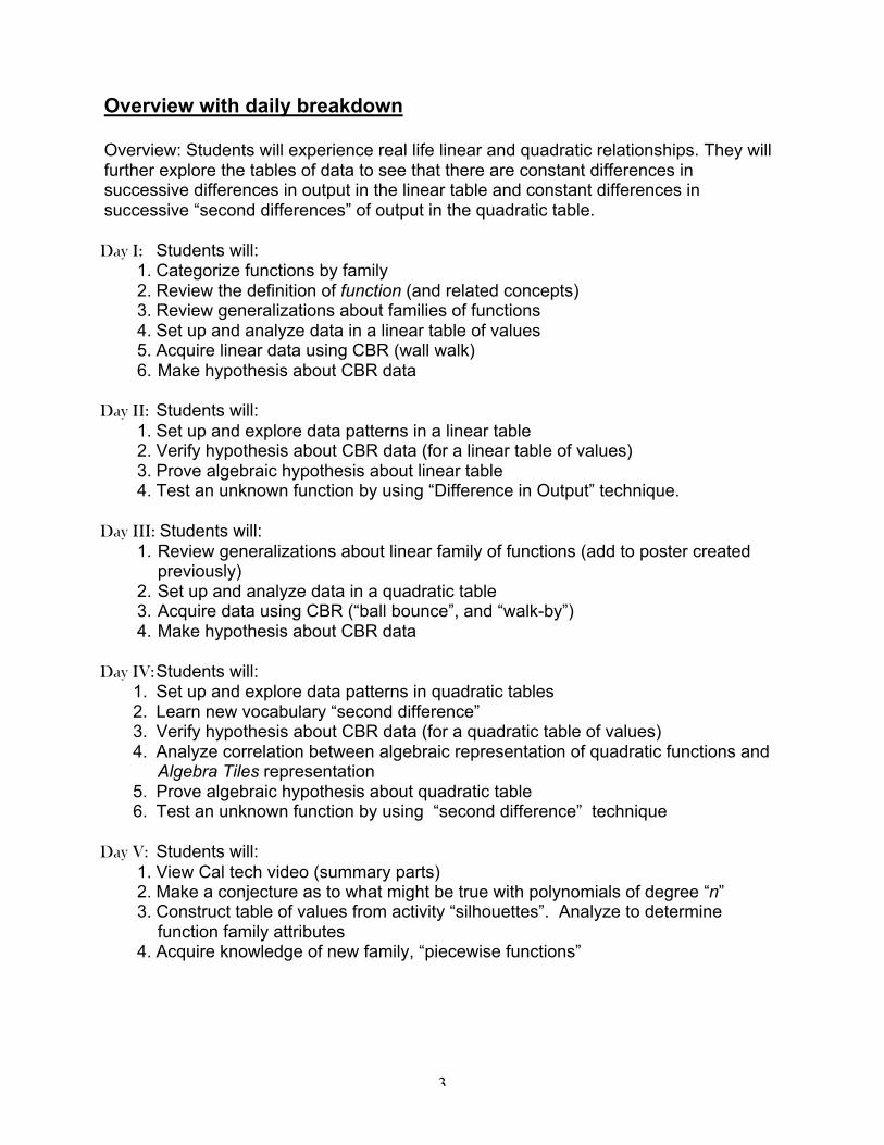
Clarify that they understand the column on the left is what goes “in” to the function

(independent variable) and the right is what goes “out” of the function (dependent

variable). They may want to draw arrows.

D. Acquire linear data using CBR (walking) / make hypothesis about CBR data)

For teachers that can get the use of only one CBR, arrange the class into four

heterogeneous groups. Two of the groups at a time will watch and participate in data

collection. The other two groups will work separately on the first homework problem

[264: #1. a, c; #2. a, c]. The first two groups will record on the CBR, “walking” away from

the CBR. The second group will record, “walking” towards the CBR. This is similar to

the data collection stage of “Activity 3” p. 11 in Modeling Motion: High School Math

Activities with the CBR. If you need to brush up on your CBR skills there is a nice

refresher on p. vii of Modeling Motion: High School Math Activities with the CBR. The

CBR requires room enough for true readings. If you cannot clear a path of about 10 feet

long and 6 feet wide, then the activity will probably need to be done in the hall.

Tell them that you are going to record the distance that the participant is away

from the CBR at very small time intervals (every fraction of second). Have them huddle

as a group and guess the shape of the forthcoming graph. Acquire the data; let them

see the graph, then repeat with the next group except substitute “walking towards” the

CBR for “walking away from” (and start about 10 feet away). Save the data from the

first run because the CBR will override the data from the second run if you do not. I

In Out

1 11

2 15 4

3 19 4

4 23 4

5 27 4

6 31 4

In Out

1 11

2 15

3 19

4 23

5 27

6 31

4

4

4

4

4

7

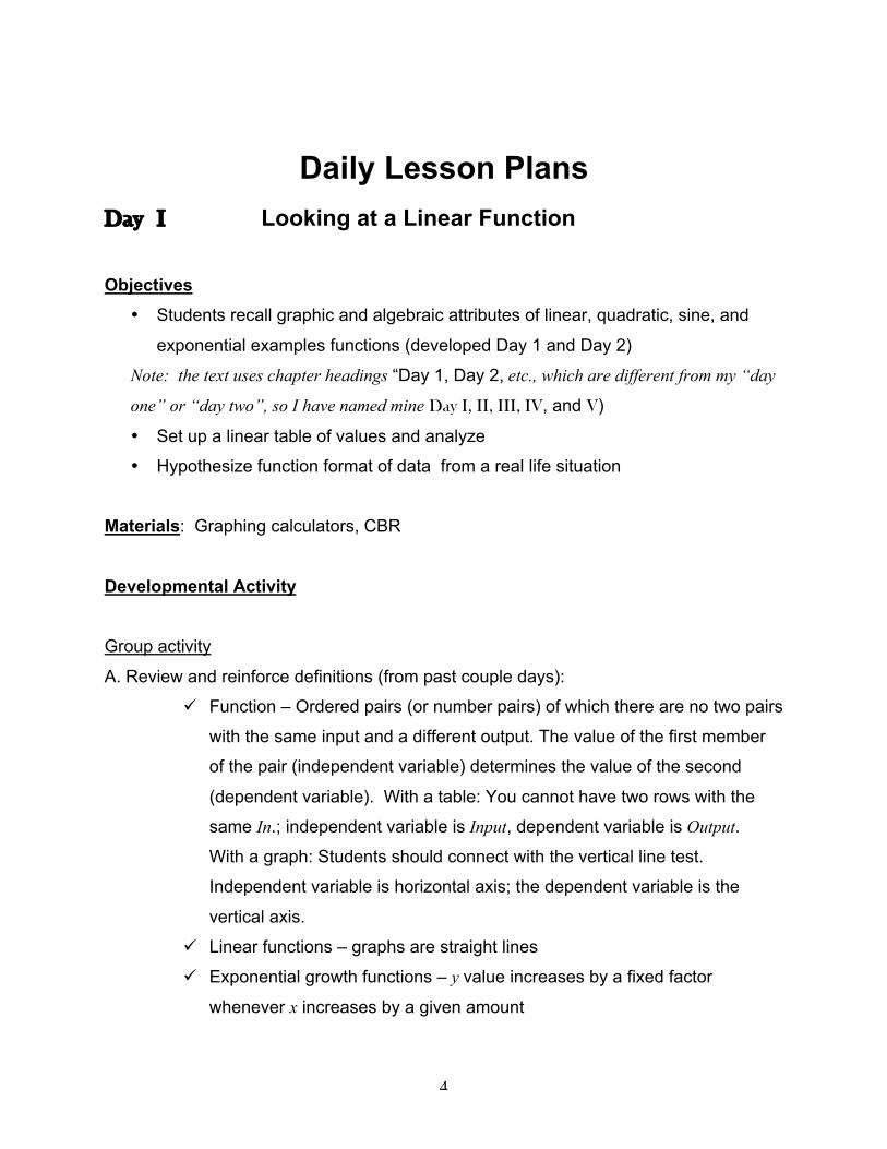
saved mine to a list named WLKF, WLKFF (walk forward). After you transmit the data

from the CBR to the calculator, the data is stored in lists 1 through 4. We are using time

and distance, L1 and L2. To save them after the first capture, go to the home screen

and enter L1 / STO> / WLKFF / ENTER and L2 / STO> / WLKF / ENTER. [2ND and

the white number keys will get your lists L1 through L6]. Save the second set of data

also.

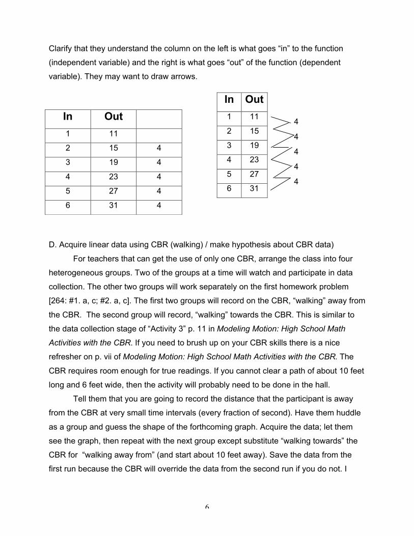
closure – As an exit ticket, have students hand in a half sheet of paper with their guess

of what the graph will look like if the participant would have held the CBR and walked

towards the wall from 10 feet away. (It should be linear with negative slope)

Homework p. 264: #1. a, c; #2. a, c (not b)

AT THE END OF CLASS OR BEFORE TOMMORROW: store the

newly named lists back to L1, L2, L3, L4. You probably should clean up the lists before

class.

You may not have perfect data (as I did not). I did have a real nice section (that I

circled here). We want to get a table for them to work with, and let the calculator do the

calculations for them in terms of the differences in output. We will do this by creating

8

two output lists. The second list will be the same as the first, only shifted by one

position. We will then let the students take the difference of the two lists.

Press LIST, arrow to OPS/ 8 (SELECT)/ENTER (this brings you to home screen.

Inside the Select parenthesis enter your desired independent x list, dependent y list.

This will be the same as what your graph was L1, L2. I will explain using L1 and L2, it

will be the same for L3 and L4 for the backward group. ENTER and you will be brought

back to the graph. Arrow when prompted to the appropriate left and right bounds of

“good data”. Hit ENTER. Now you have a smaller L1, and L2. In the same way, correct

lists L3 and L4.Transmit these lists to the students.

9

Day II Proving the Linear Table Pattern

Objectives

• Apply a function to a real life situation

• Apply “Difference in Output” technique to verify a linear relationship (given

expression and CBR data)

• Prove algebraic hypothesis about “Difference in Output” in linear table

• Analyze an unknown function for linearity by using “Difference in Output”technique

• Develop skill at managing a table of data and plotting its graph on the graphingcalculator

Materials: Graphing calculators, CBR

Developmental Activity

Group activity

A. Review homework:

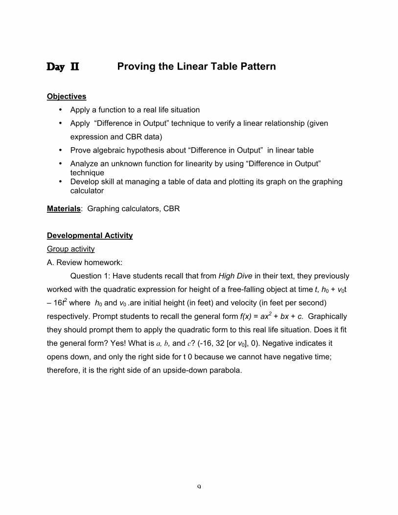
Question 1: Have students recall that from High Dive in their text, they previously

worked with the quadratic expression for height of a free-falling object at time t, h0 + v0t

– 16t2 where h0 and v0 .are initial height (in feet) and velocity (in feet per second)

respectively. Prompt students to recall the general form f(x) = ax2 + bx + c. Graphically

they should prompt them to apply the quadratic form to this real life situation. Does it fit

the general form? Yes! What is a, b, and c? (-16, 32 [or v0], 0). Negative indicates it

opens down, and only the right side for t 0 because we cannot have negative time;

therefore, it is the right side of an upside-down parabola.

10

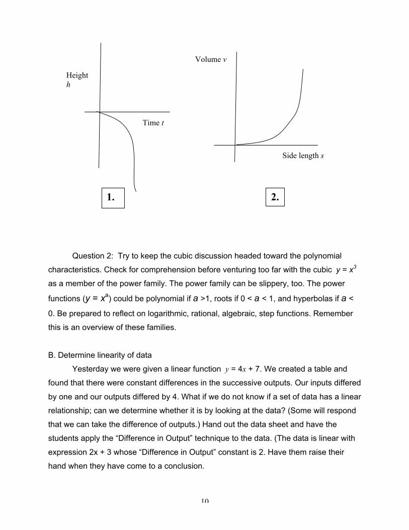
Question 2: Try to keep the cubic discussion headed toward the polynomial

characteristics. Check for comprehension before venturing too far with the cubic y = x3

as a member of the power family. The power family can be slippery, too. The power

functions (y = xa) could be polynomial if a >1, roots if 0 < a < 1, and hyperbolas if a <

0. Be prepared to reflect on logarithmic, rational, algebraic, step functions. Remember

this is an overview of these families.

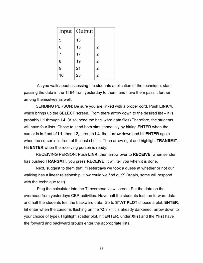
B. Determine linearity of data

Yesterday we were given a linear function y = 4x + 7. We created a table and

found that there were constant differences in the successive outputs. Our inputs differed

by one and our outputs differed by 4. What if we do not know if a set of data has a linear

relationship; can we determine whether it is by looking at the data? (Some will respond

that we can take the difference of outputs.) Hand out the data sheet and have the

students apply the “Difference in Output” technique to the data. (The data is linear with

expression 2x + 3 whose “Difference in Output” constant is 2. Have them raise their

hand when they have come to a conclusion.

Heighth

2.

Volume v

Side length s

1.

Time t

11

As you walk about assessing the students application of the technique, start

passing the data in the TI-84 from yesterday to them, and have them pass it further

among themselves as well.

SENDING PERSON: Be sure you are linked with a proper cord. Push LINK/4,

which brings up the SELECT screen. From there arrow down to the desired list – it is

probably L1 through L4. (Also, send the backward data files) Therefore, the students

will have four lists. Chose to send both simultaneously by hitting ENTER when the

cursor is in front of L1, then L2, through L4, then arrow down and hit ENTER again

when the cursor is in front of the last choice. Then arrow right and highlight TRANSMIT.

Hit ENTER when the receiving person is ready.

RECEIVING PERSON: Push LINK, then arrow over to RECEIVE, when sender

has pushed TRANSMIT, you press RECEIVE. It will tell you when it is done.

Next, suggest to them that, “Yesterdays we took a guess at whether or not our

walking has a linear relationship. How could we find out?” (Again, some will respond

with the technique test)

Plug the calculator into the TI overhead view screen. Put the data on the

overhead from yesterdays CBR activities. Have half the students test the forward data

and half the students test the backward data. Go to STAT PLOT choose a plot, ENTER,

hit enter when the cursor is flashing on the “On” (if it is already darkened, arrow down to

your choice of type). Highlight scatter plot, hit ENTER, under Xlist and the Ylist have

the forward and backward groups enter the appropriate lists.

Input Output

5 13

6 15 2

7 17 2

8 19 2

9 21 2

10 23 2

12

One option is let the students record (on a written table) each difference for a

successive group of values. This can be done by having the students pick out about five

or six values from the output list. The entry number from the list can be found as they

scroll through the table. The entry number is revealed at the bottom left of the screen

with its value. E.g. L2(1) = 13.651. So on the homescreen the students can manually

enter L2(n +1) – L2(n) and begin recording the differences in output with equally

spaced successive values of n.

Another option is to go to the home screen and store L2 to L3. Go back to STAT/

EDIT and scroll to the top of L2 column. Highlight the first entry and delete it by

pressing DEL. Then delete the last entry in L3. (Scrolling up is probably quicker). Now

take the difference of these two lists from the home screen (L3-L2). This will give the

students all the differences in output. They can arrow right and left to see the whole set.

If they leave the screen or hit ENTER they will lose the ability to scroll through the

results. Although it is easy to regenerate. You can show them another way in Excel as I

will explain using the quadratic on Day IV

The bottom line…is the data reflective of a linear function? Either answer could

be correct. Have the students justify their answer. If time permits, the students could

bring their calculators up front, plug into the overhead, and explain their reasoning. It

may be more apparent to them how close it is if you have them go in MODE and in the

second row choose 1 decimal place, then recalculate the data.

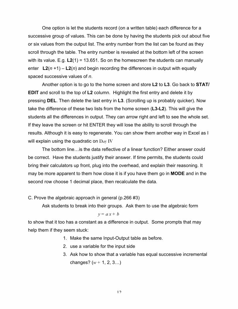
C. Prove the algebraic approach in general (p.266 #3)

Ask students to break into their groups. Ask them to use the algebraic form

y = a x + b

to show that it too has a constant as a difference in output. Some prompts that may

help them if they seem stuck:

1. Make the same Input-Output table as before.

2. use a variable for the input side

3. Ask how to show that a variable has equal successive incremental

changes? (w + 1, 2, 3…)

13

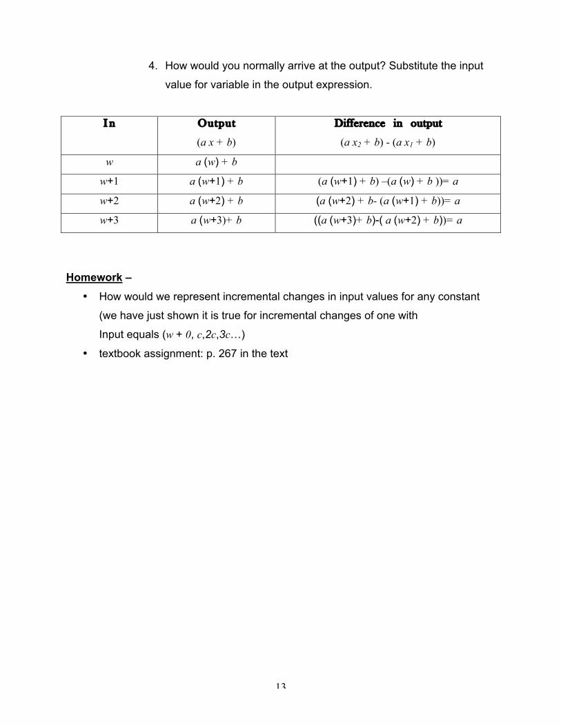
4. How would you normally arrive at the output? Substitute the input

value for variable in the output expression.

I n Output

(a x + b)

Difference in output

(a x2 + b) - (a x1 + b)

w a (w) + b

w+1 a (w+1) + b (a (w+1) + b) –(a (w) + b ))= a

w+2 a (w+2) + b (a (w+2) + b- (a (w+1) + b))= a

w+3 a (w+3)+ b ((a (w+3)+ b)-( a (w+2) + b))= a

Homework –

• How would we represent incremental changes in input values for any constant

(we have just shown it is true for incremental changes of one with

Input equals (w + 0, c,2c,3c…)

• textbook assignment: p. 267 in the text

14

Day III Looking at a Quadratic Function

Objectives

• Practice mathematical reasoning in an algebraic proof

• Analyze a situation in order to represent it with a function

• Discover “second difference” as a measurable attribute of quadratics.

• Practice logical and critical thinking with abstract variables in a proof.

Developmental Activity

Group activity

A. Review homework:

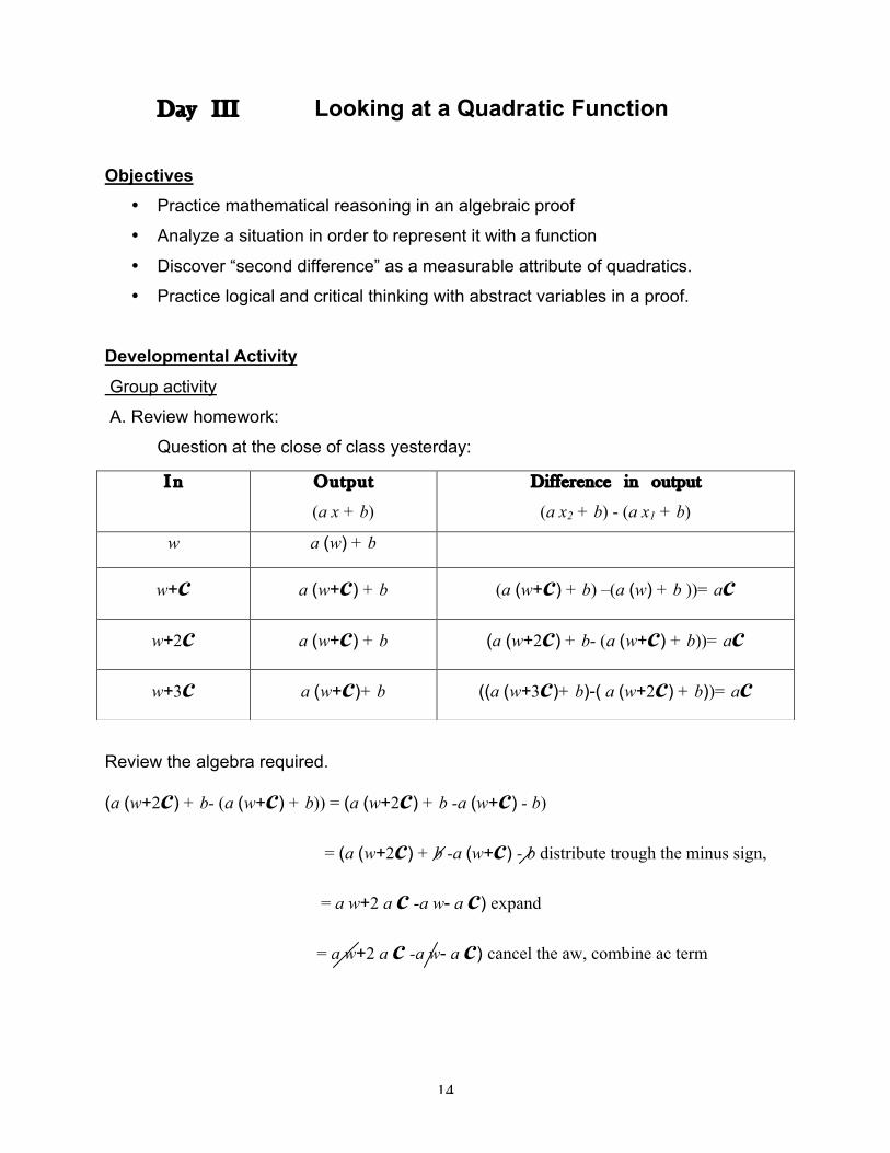
Question at the close of class yesterday:

Review the algebra required.

(a (w+2c) + b- (a (w+c) + b)) = (a (w+2c) + b -a (w+c) - b)

= (a (w+2c) + b -a (w+c) - b distribute trough the minus sign,

= a w+2 a c -a w- a c) expand

= a w+2 a c -a w- a c) cancel the aw, combine ac term

I n Output

(a x + b)

Difference in output

(a x2 + b) - (a x1 + b)

w a (w) + b

w+c a (w+c) + b (a (w+c) + b) –(a (w) + b ))= ac

w+2c a (w+c) + b (a (w+2c) + b- (a (w+c) + b))= ac

w+3c a (w+c)+ b ((a (w+3c)+ b)-( a (w+2c) + b))= ac

15

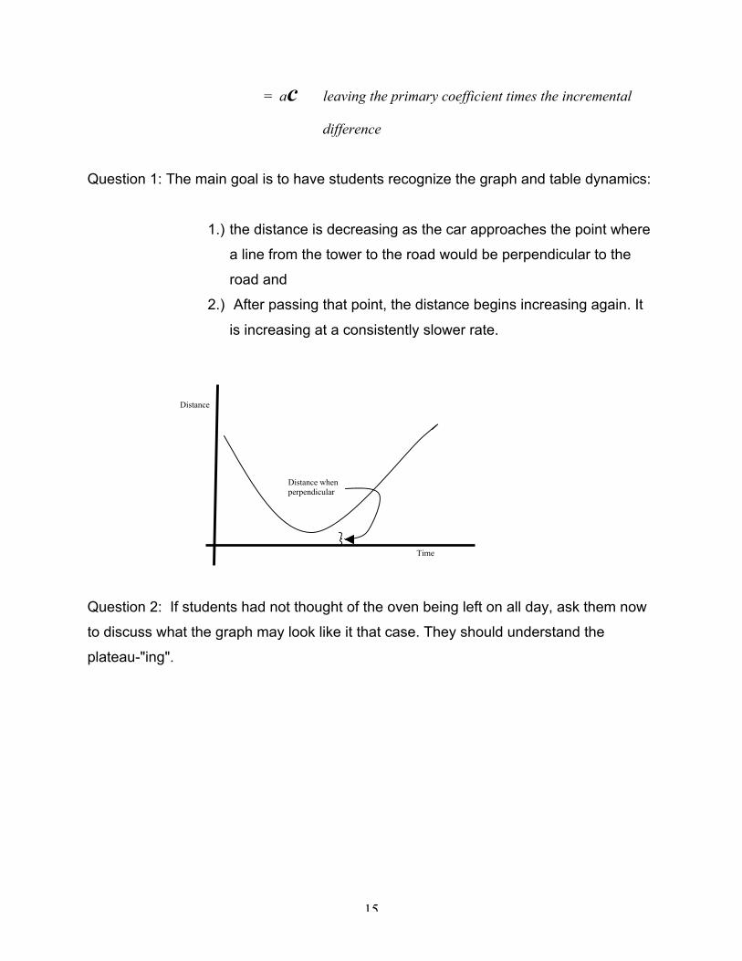
= ac leaving the primary coefficient times the incremental

difference

Question 1: The main goal is to have students recognize the graph and table dynamics:

1.) the distance is decreasing as the car approaches the point where

a line from the tower to the road would be perpendicular to the

road and

2.) After passing that point, the distance begins increasing again. It

is increasing at a consistently slower rate.

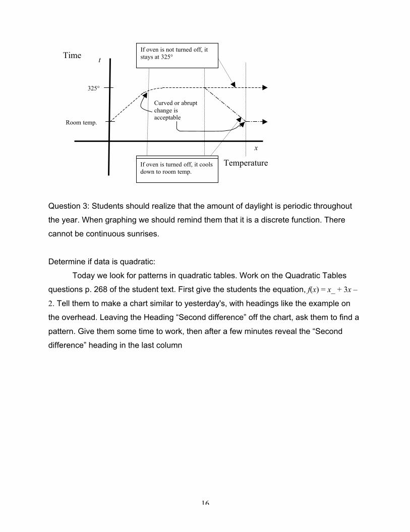
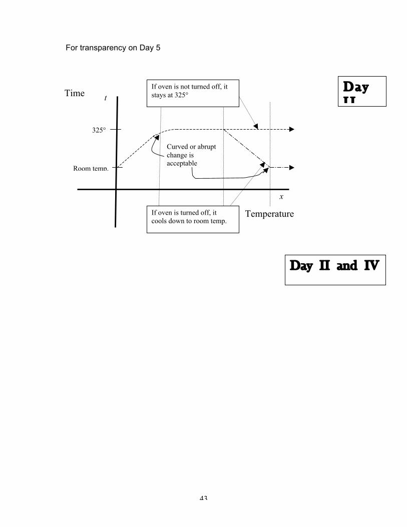
Question 2: If students had not thought of the oven being left on all day, ask them now

to discuss what the graph may look like it that case. They should understand the

plateau-"ing".

Time

Distance

Distance whenperpendicular

16

Question 3: Students should realize that the amount of daylight is periodic throughout

the year. When graphing we should remind them that it is a discrete function. There

cannot be continuous sunrises.

Determine if data is quadratic:

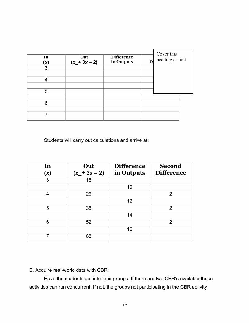
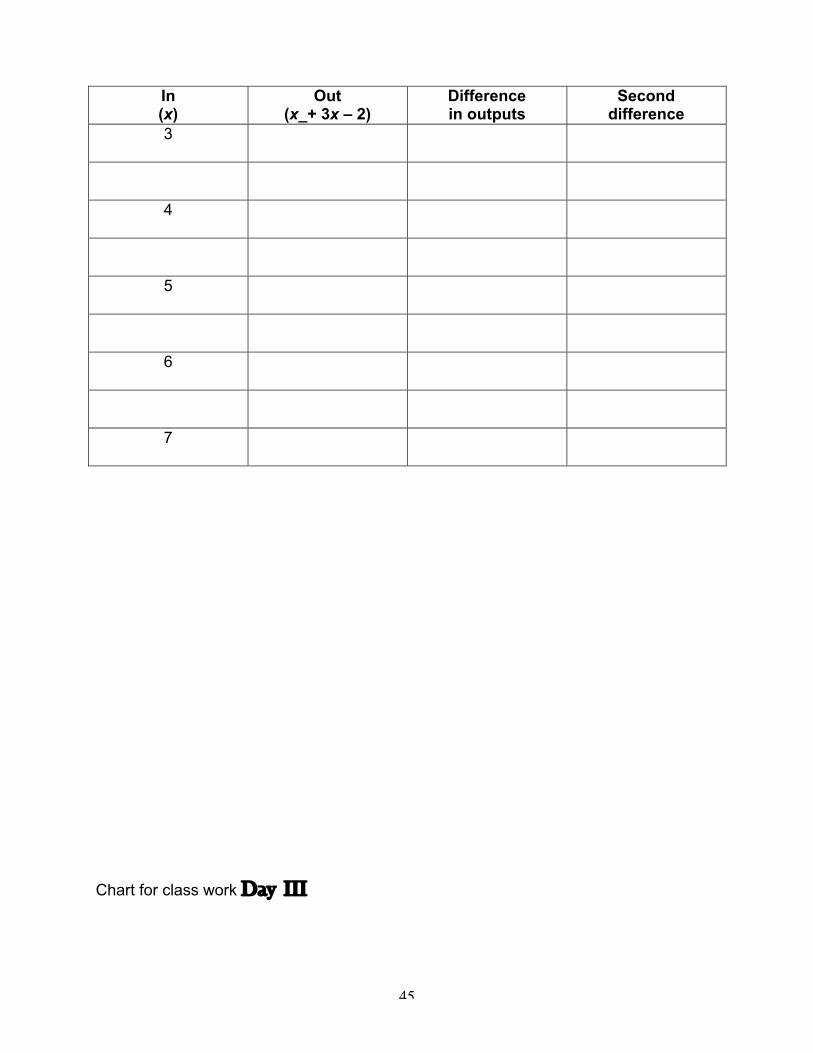
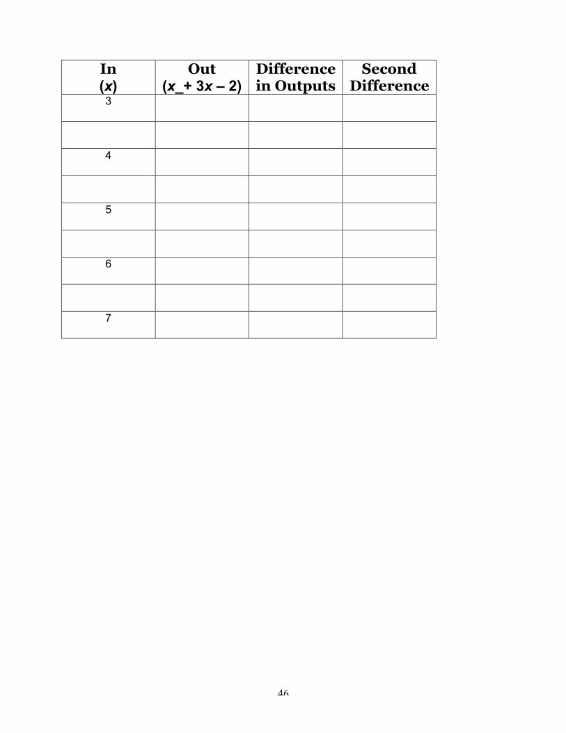
Today we look for patterns in quadratic tables. Work on the Quadratic Tables

questions p. 268 of the student text. First give the students the equation, f(x) = x_ + 3x –

2. Tell them to make a chart similar to yesterday's, with headings like the example on

the overhead. Leaving the Heading “Second difference” off the chart, ask them to find a

pattern. Give them some time to work, then after a few minutes reveal the “Second

difference” heading in the last column

x

If oven is turned off, it coolsdown to room temp.

325°

Curved or abruptchange isacceptable

t

Room temp.

If oven is not turned off, itstays at 325°Time

TemperatureIf oven is turned off, it coolsdown to room temp.

17

In(x)

Out(x_+ 3x – 2)

Differencein Outputs

SecondDifference

3

4

5

6

7

Students will carry out calculations and arrive at:

In(x)

Out(x_+ 3x – 2)

Differencein Outputs

SecondDifference

3 16

10

4 26 2

12

5 38 2

14

6 52 2

16

7 68

B. Acquire real-world data with CBR:

Have the students get into their groups. If there are two CBR’s available these

activities can run concurrent. If not, the groups not participating in the CBR activity

Cover thisheading at first

18

begin their homework (p. 269-270: 1-4 emphasize preliminary instructions in book

regarding analysis for feasibility of available data.).

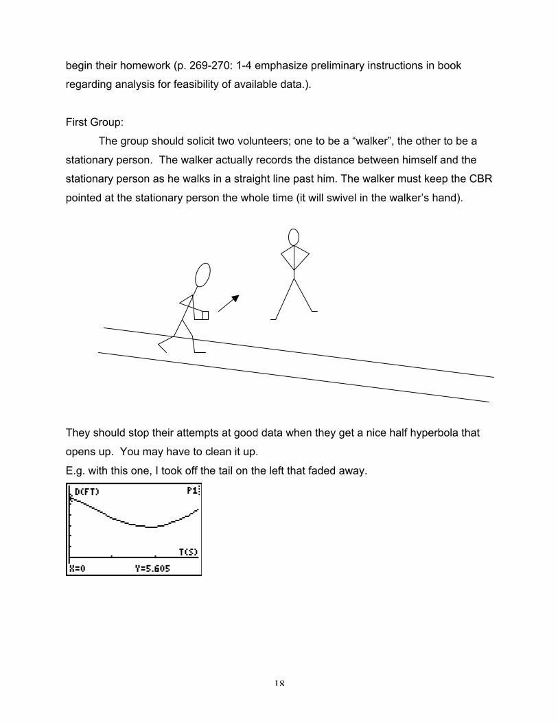
First Group:

The group should solicit two volunteers; one to be a “walker”, the other to be a

stationary person. The walker actually records the distance between himself and the

stationary person as he walks in a straight line past him. The walker must keep the CBR

pointed at the stationary person the whole time (it will swivel in the walker’s hand).

They should stop their attempts at good data when they get a nice half hyperbola that

opens up. You may have to clean it up.

E.g. with this one, I took off the tail on the left that faded away.

19

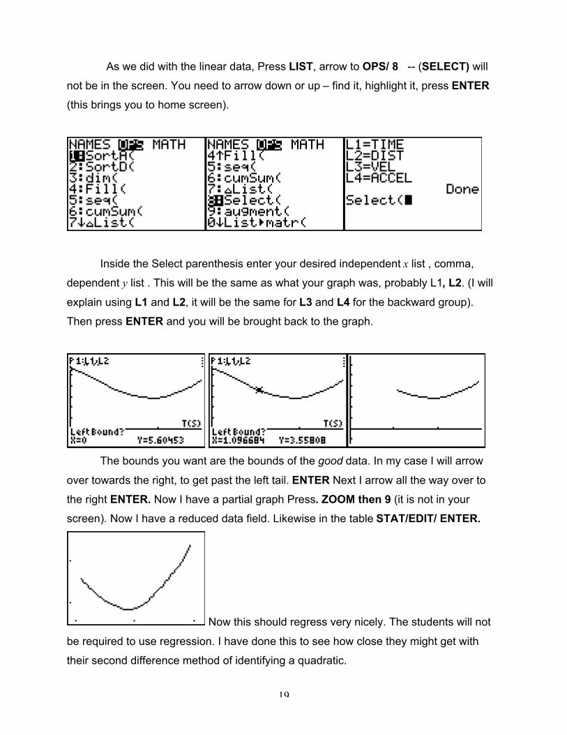
As we did with the linear data, Press LIST, arrow to OPS/ 8 -- (SELECT) will

not be in the screen. You need to arrow down or up – find it, highlight it, press ENTER

(this brings you to home screen).

Inside the Select parenthesis enter your desired independent x list , comma,

dependent y list . This will be the same as what your graph was, probably L1, L2. (I will

explain using L1 and L2, it will be the same for L3 and L4 for the backward group).

Then press ENTER and you will be brought back to the graph.

The bounds you want are the bounds of the good data. In my case I will arrow

over towards the right, to get past the left tail. ENTER Next I arrow all the way over to

the right ENTER. Now I have a partial graph Press. ZOOM then 9 (it is not in your

screen). Now I have a reduced data field. Likewise in the table STAT/EDIT/ ENTER.

Now this should regress very nicely. The students will not

be required to use regression. I have done this to see how close they might get with

their second difference method of identifying a quadratic.

20

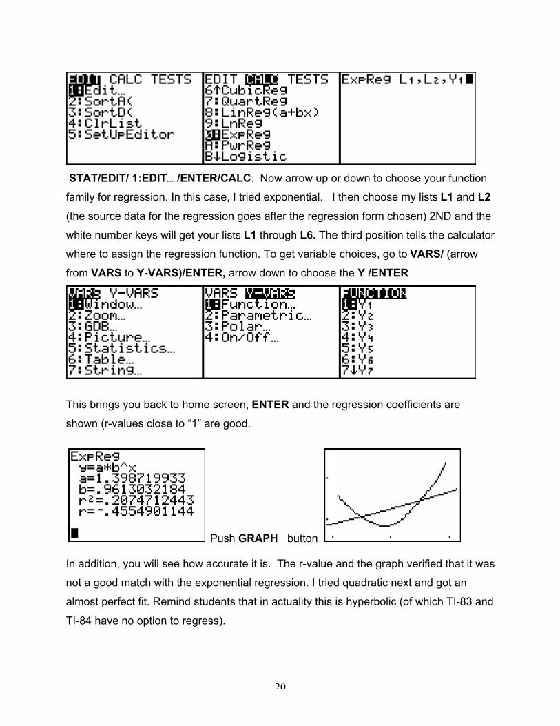
STAT/EDIT/ 1:EDIT… /ENTER/CALC. Now arrow up or down to choose your function

family for regression. In this case, I tried exponential. I then choose my lists L1 and L2

(the source data for the regression goes after the regression form chosen) 2ND and the

white number keys will get your lists L1 through L6. The third position tells the calculator

where to assign the regression function. To get variable choices, go to VARS/ (arrow

from VARS to Y-VARS)/ENTER, arrow down to choose the Y /ENTER

This brings you back to home screen, ENTER and the regression coefficients are

shown (r-values close to “1” are good.

Push GRAPH button In addition, you will see how accurate it is. The r-value and the graph verified that it was

not a good match with the exponential regression. I tried quadratic next and got an

almost perfect fit. Remind students that in actuality this is hyperbolic (of which TI-83 and

TI-84 have no option to regress).

21

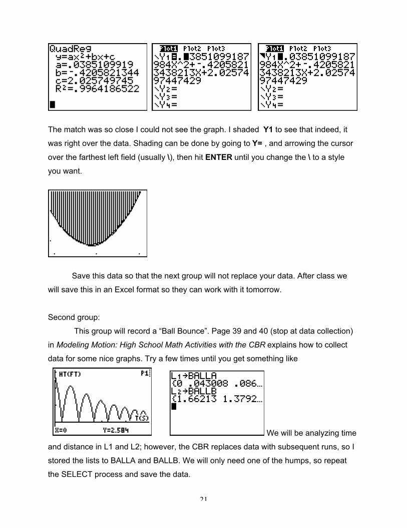
The match was so close I could not see the graph. I shaded Y1 to see that indeed, it

was right over the data. Shading can be done by going to Y= , and arrowing the cursor

over the farthest left field (usually \), then hit ENTER until you change the \ to a style

you want.

Save this data so that the next group will not replace your data. After class we

will save this in an Excel format so they can work with it tomorrow.

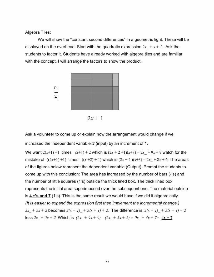
Second group:

This group will record a “Ball Bounce”. Page 39 and 40 (stop at data collection)

in Modeling Motion: High School Math Activities with the CBR explains how to collect

data for some nice graphs. Try a few times until you get something like

We will be analyzing time

and distance in L1 and L2; however, the CBR replaces data with subsequent runs, so I

stored the lists to BALLA and BALLB. We will only need one of the humps, so repeat

the SELECT process and save the data.

22

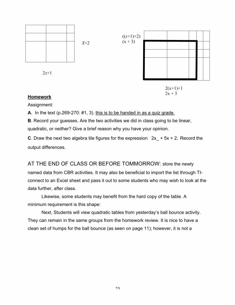
Algebra Tiles:

We will show the “constant second differences” in a geometric light. These will be

displayed on the overhead. Start with the quadratic expression 2x_ + x + 2. Ask the

students to factor it. Students have already worked with algebra tiles and are familiar

with the concept. I will arrange the factors to show the product.

Ask a volunteer to come up or explain how the arrangement would change if we

increased the independent variable x (input) by an increment of 1.

We want 2(x+1) +1 times (x+1) + 2 which is (2x + 2 +1)(x+3) = 2x_ + 9x + 9 watch for the

mistake of ((2x+1) +1) times ((x +2) + 1) which is (2x + 2 )(x+3) = 2x_ + 8x + 6. The areas

of the figures below represent the dependent variable (Output). Prompt the students to

come up with this conclusion: The area has increased by the number of bars (x’s) and

the number of little squares (1’s) outside the thick lined box. The thick lined box

represents the initial area superimposed over the subsequent one. The material outside

is 4 x’s and 7 (1’s). This is the same result we would have if we did it algebraically.

(It is easier to expand the expression first then implement the incremental change.)

2x_ + 5x + 2 becomes 2(x + 1)_ + 5(x + 1) + 2. The difference is 2(x + 1)_ + 5(x + 1) + 2

less 2x_ + 5x + 2. Which is (2x_ + 9x + 9) – (2x_ + 5x + 2) = 0x_ + 4x + 7= 4x + 7

2x + 1

23

2x+1

Homework

Assignment:

A. In the text (p.269-270: #1, 3). this is to be handed in as a quiz grade.

B. Record your guesses. Are the two activities we did in class going to be linear,

quadratic, or neither? Give a brief reason why you have your opinion.

C. Draw the next two algebra tile figures for the expression 2x_ + 5x + 2. Record the

output differences.

AT THE END OF CLASS OR BEFORE TOMMORROW: store the newly

named data from CBR activities. It may also be beneficial to import the list through TI-

connect to an Excel sheet and pass it out to some students who may wish to look at the

data further, after class.

Likewise, some students may benefit from the hard copy of the table. A

minimum requirement is this shape:

Next, Students will view quadratic tables from yesterday’s ball bounce activity.

They can remain in the same groups from the homework review. It is nice to have a

clean set of humps for the ball bounce (as seen on page 11); however, it is not a

X+2

((x+1)+2)(x + 3)

2(x+1)+12x + 3

24

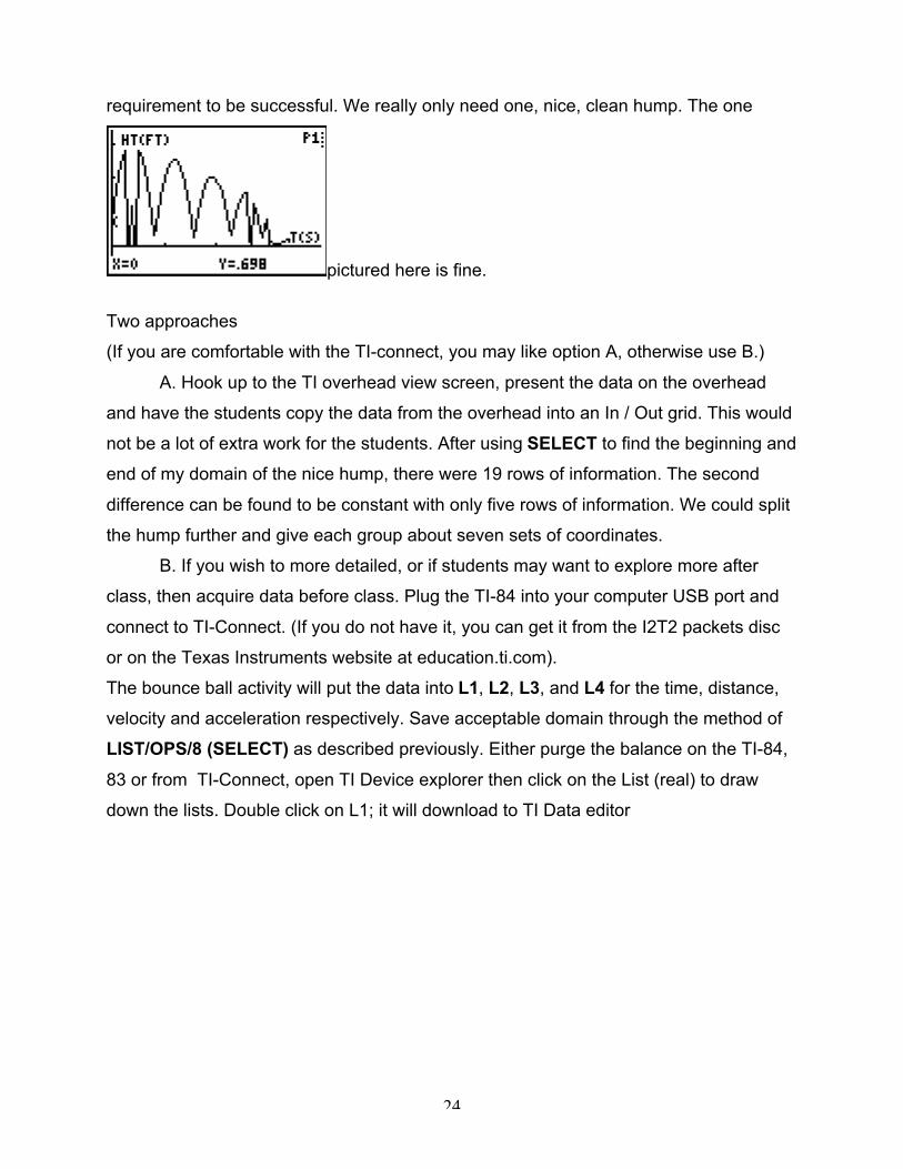
requirement to be successful. We really only need one, nice, clean hump. The one

pictured here is fine.

Two approaches

(If you are comfortable with the TI-connect, you may like option A, otherwise use B.)

A. Hook up to the TI overhead view screen, present the data on the overhead

and have the students copy the data from the overhead into an In / Out grid. This would

not be a lot of extra work for the students. After using SELECT to find the beginning and

end of my domain of the nice hump, there were 19 rows of information. The second

difference can be found to be constant with only five rows of information. We could split

the hump further and give each group about seven sets of coordinates.

B. If you wish to more detailed, or if students may want to explore more after

class, then acquire data before class. Plug the TI-84 into your computer USB port and

connect to TI-Connect. (If you do not have it, you can get it from the I2T2 packets disc

or on the Texas Instruments website at education.ti.com).

The bounce ball activity will put the data into L1, L2, L3, and L4 for the time, distance,

velocity and acceleration respectively. Save acceptable domain through the method of

LIST/OPS/8 (SELECT) as described previously. Either purge the balance on the TI-84,

83 or from TI-Connect, open TI Device explorer then click on the List (real) to draw

down the lists. Double click on L1; it will download to TI Data editor

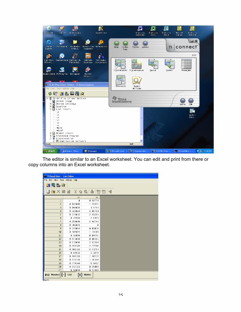
25

The editor is similar to an Excel worksheet. You can edit and print from there orcopy columns into an Excel worksheet.

26

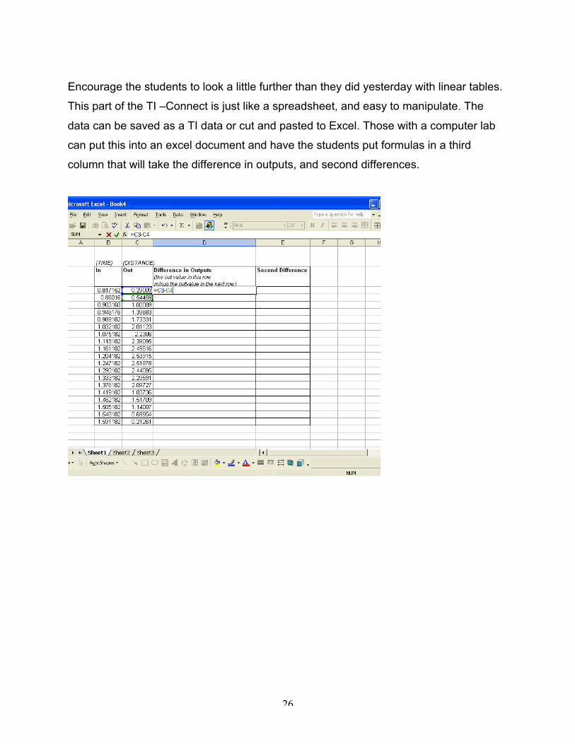
Encourage the students to look a little further than they did yesterday with linear tables.

This part of the TI –Connect is just like a spreadsheet, and easy to manipulate. The

data can be saved as a TI data or cut and pasted to Excel. Those with a computer lab

can put this into an excel document and have the students put formulas in a third

column that will take the difference in outputs, and second differences.

27

Day IV Proving the Quadratic Table Pattern

Objectives

• students will apply attributes learned so that they can sense how a situation,

graph , or table fits into a family

• Determine if a table of values exhibit attributes of a linear function by analyzing

algebraic, graphic, and table attributes

• Discuss homework (students will apply attributes learned so that they can sense

how a situation, graph , or table fits into a family)

• Prove algebraic hypothesis about relationship among output values in a

quadratic function. [Using general form with variables]

Materials: Graphing calculators, CBR, computer (excel, TI-Connect)

Developmental Activity

Group activity:

Homework Review

Assignment: To be handed in as a quiz grade.

A. p.269-270: (1) the homework/quiz is not regarded heavily towards their grade. It

would not be monitored closely for sharing ideas, and is in fact hoped that they would

get together and share ideas. The main purpose is to see if they are on track, and to

encourage regular, routine participation.

Question 1: If the students assume the sale of 30 items to a linear function, then

they would need to verify it fits in the y = mx + b form. If C is cost and Q is quantity,

then C = (388.50/30)Q or C = 12.95Q. To fit this would require an assumption that zero

calculators cost $0, which is fine. A student would get extra credit if he/she took into

consideration the fact that schools may get a break in price at certain volumes, thus be

a composite of a few connected linear parts., or volume discounts, or there may be a

flat rate for shipping which would cause the equation to have a b value.

28

They might mention that schools should be exempt from tax. These factors would affect

the function. Credit would be awarded to students with the basic equation. The

students could present a feasible graph or table for credit also..

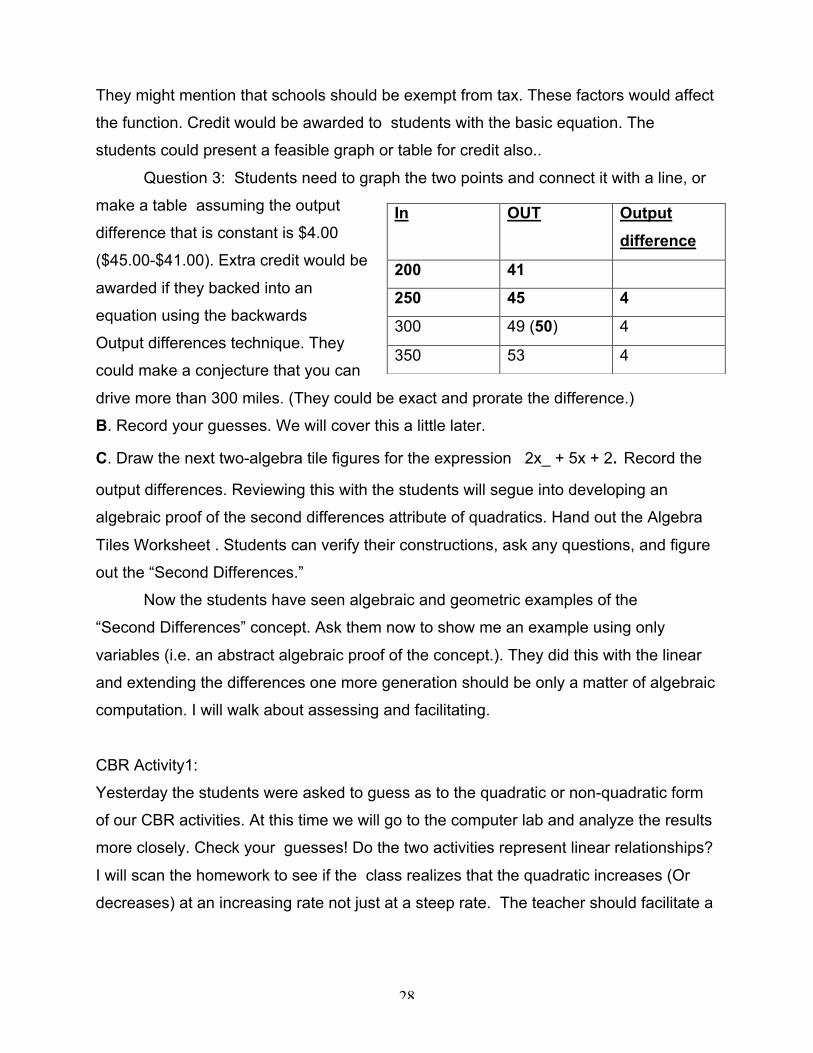
Question 3: Students need to graph the two points and connect it with a line, or

make a table assuming the output

difference that is constant is $4.00

($45.00-$41.00). Extra credit would be

awarded if they backed into an

equation using the backwards

Output differences technique. They

could make a conjecture that you can

drive more than 300 miles. (They could be exact and prorate the difference.)

B. Record your guesses. We will cover this a little later.

C. Draw the next two-algebra tile figures for the expression 2x_ + 5x + 2. Record the

output differences. Reviewing this with the students will segue into developing an

algebraic proof of the second differences attribute of quadratics. Hand out the Algebra

Tiles Worksheet . Students can verify their constructions, ask any questions, and figure

out the “Second Differences.”

Now the students have seen algebraic and geometric examples of the

“Second Differences” concept. Ask them now to show me an example using only

variables (i.e. an abstract algebraic proof of the concept.). They did this with the linear

and extending the differences one more generation should be only a matter of algebraic

computation. I will walk about assessing and facilitating.

CBR Activity1:

Yesterday the students were asked to guess as to the quadratic or non-quadratic form

of our CBR activities. At this time we will go to the computer lab and analyze the results

more closely. Check your guesses! Do the two activities represent linear relationships?

I will scan the homework to see if the class realizes that the quadratic increases (Or

decreases) at an increasing rate not just at a steep rate. The teacher should facilitate a

In OUT Output

difference

200 41

250 45 4

300 49 (50) 4

350 53 4

29

short discussion being sure to include the fact that in both examples the rate of change

was NOT constant and a quadratic model would be appropriate for both.

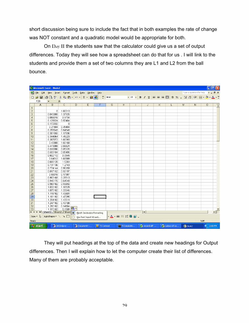
On Day II the students saw that the calculator could give us a set of output

differences. Today they will see how a spreadsheet can do that for us . I will link to the

students and provide them a set of two columns they are L1 and L2 from the ball

bounce.

They will put headings at the top of the data and create new headings for Output

differences. Then I will explain how to let the computer create their list of differences.

Many of them are probably acceptable.

30

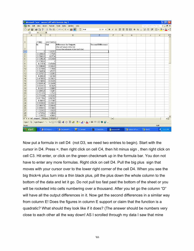
Now put a formula in cell D4 (not D3, we need two entries to begin). Start with the

cursor in D4. Press =, then right click on cell C4, then hit minus sign , then right click on

cell C3. Hit enter, or click on the green checkmark up in the formula bar. You don not

have to enter any more formulas. Right click on cell D4. Pull the big plus sign that

moves with your cursor over to the lower right corner of the cell D4. When you see the

big thick=k plus turn into a thin black plus, pill the plus down the whole column to the

bottom of the data and let it go. Do not pull too fast past the bottom of the sheet or you

will be rocketed into cells numbering over a thousand. After you let go the column “D”

will have all the output differences in it. Now get the second differences in a similar way

from column E! Does the figures in column E support or claim that the function is a

quadratic? What should they look like if it does? (The answer should be numbers very

close to each other all the way down! AS I scrolled through my data I saw that mine

31

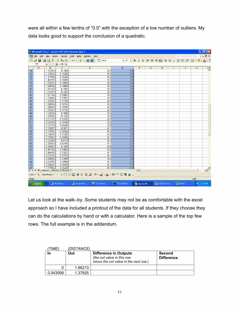
were all within a few tenths of “0.0” with the exception of a low number of outliers. My

data looks good to support the conclusion of a quadratic.

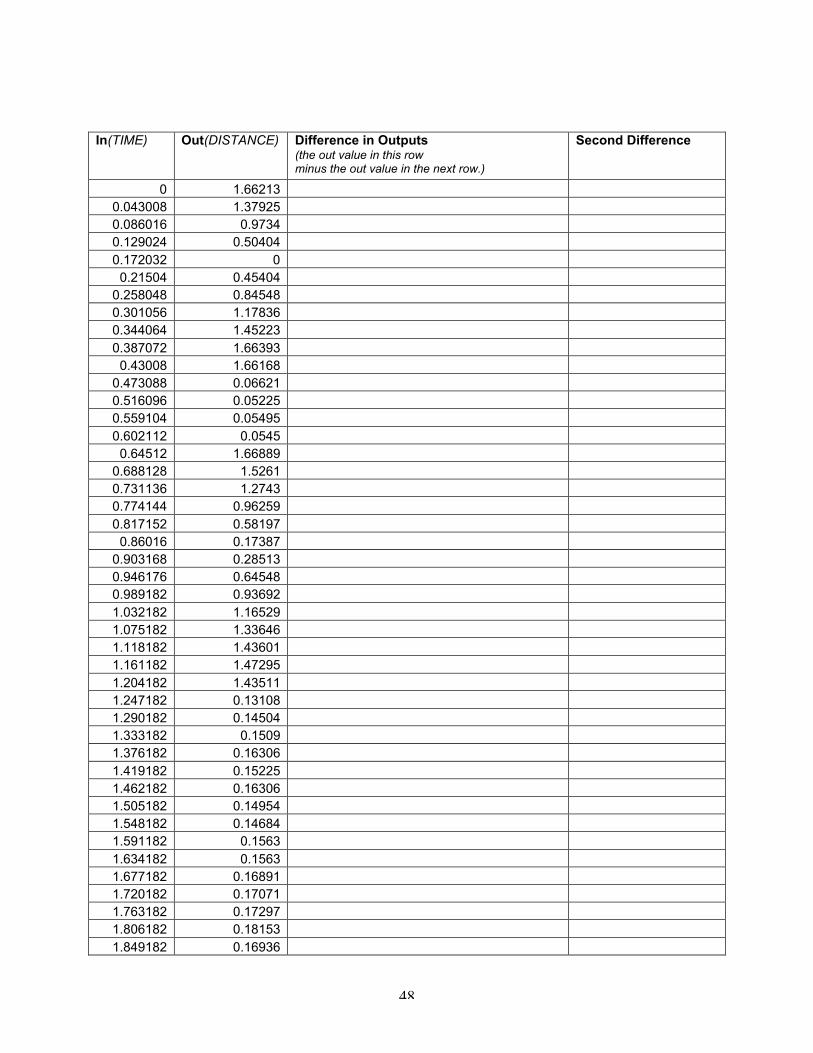
Let us look at the walk–by. Some students may not be as comfortable with the excel

approach so I have included a printout of the data for all students. If they choose they

can do the calculations by hand or with a calculator. Here is a sample of the top few

rows. The full example is in the addendum.

(TIME) (DISTANCE)In Out Difference in Outputs

(the out value in this rowminus the out value in the next row.)

SecondDifference

0 1.66213 0.043008 1.37925

32

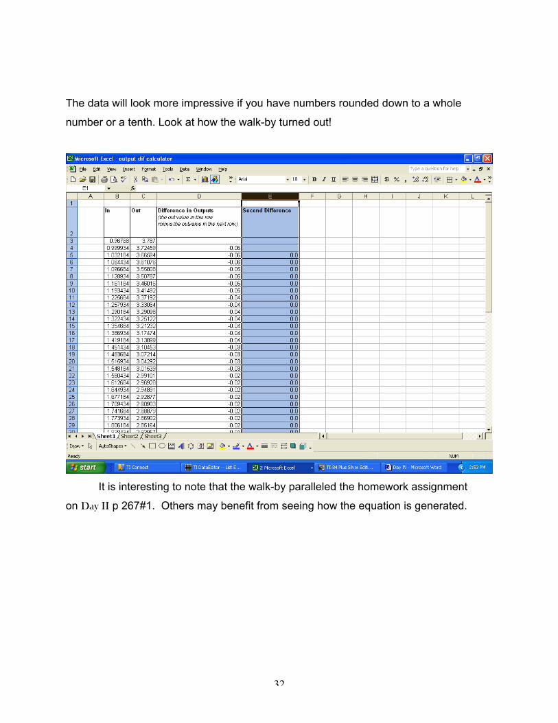
The data will look more impressive if you have numbers rounded down to a whole

number or a tenth. Look at how the walk-by turned out!

It is interesting to note that the walk-by paralleled the homework assignment

on Day II p 267#1. Others may benefit from seeing how the equation is generated.

33

We start with h_ = f _ + g_ where c is the desired independent variable, g = r_t where r

is the rate the car is traveling in mph, t is the time in hours he travels along the road.

Substitution gives us y f r t= + ⋅2 2( ) Showing a quick algebraic limit of

each as time approaches zero may be an easy reinforcement of yesterday. The limit of

the hyperbolic will be a constant (in this case the length f. The limit of the quadratic will

be infinite).

C. Prove algebraic hypothesis about relationship among output values in a quadratic

function. [Using general form with variables]

Ask students to break into their groups. Ask them to use the algebraic form

y = a x_ + bx + c

In order to show that this generic quadratic form always has constant second

differences when the input values are listed in equal increments.

fa

hc

g

34

Some prompts that may help them if they seem stuck:

• Make the same Input-Output table as before.

• use a variable for the input side

• Ask how to show that a variable has equal successive

incremental changes? (w +1,2,3…)

• How would you normally arrive at the output? Substitute the

input value for variable in the output expression.

I n Output

ax_ + bx + c

Difference in output

(ax2_ + b x2 + c) - (ax1_ + b x1 + c)

Second

Difference

w (w)_ + b(w) + c

w+1 a(w+1)_ + b(w+1) + c (a(w+1)_ + b(w+1)+ c) –( a(w)_ + b(w) + c)

2 a w + a + b

w+2 (w+2)_ + b(w+2) + c (a(w+2 w)_ + b(w+2)+ c) - (a(w+1)_ + b(w+1)+ c) 2 a

2 a w +3 a + b

w+3 a(w+3)_+ b(w+3) + c ((a(w+3)_+ b(w+3)+ c)-( a(w+2)_ + b (w+2)+ c)) 2 a

2 a w +5a + b

Homework – See if the second difference algorithm holds for a composite function.

Find second difference of the function x_-3x +2, when input values are 2x + 5, and x

determines the increment increases of 2x +5 by increasing by one per increment. (How

do we determine the input increment changes for the output x_-3x +2 ?, Hint: make an

extra column on the left).

35

Day V I Have a Polynomial Pattern !

Objectives

1. Understand Range and Domain and their effect on functions

2. Model real life with mathematical representation

3. Students use communication skills to discuss how and why to

break their function into pieces (introduce new name) “piecewise

functions”

4. explore “humps” and polynomial degree (remember calculator only

does regression up to 4th degree poly)

Developmental Activity

Go over homework:

See if the second difference algorithm holds for a composite function. Find

second difference of the function x_-3x +2, when input values are 2x + 5, and x

determines the increment increases of 2x + 5 by increasing by one per increment. (How

do we determine the input increment changes for the output x_-3x + 2 ? Hint: make an

extra column on the left)

• Make a table (an extra column may help students keep organized)

• The concept is not hard . Fill in the variables with an expression and

perform a lot of calculations

• Take your time

• Be neat

36

I n

bas i s

I n Output

ax_ + bx + c

Difference in output

(ax2_ + b x2 + c) - (ax1_ + b x1 + c)

Second

Difference

0 w (w)_ + b(w) + c

1 w+1 a(w+1)_ + b(w+1) +

c

(a(w+1)_ + b(w+1)+ c) –( a(w)_ + b(w) + c)

2 a w + a + b

2 w+2 (w+2)_ + b(w+2) + c (a(w+2 w)_ + b(w+2)+ c) - (a(w+1)_ + b(w+1)+ c) 2 a

2 a w +3 a + b

3 w+3 a(w+3)_+ b(w+3) + c ((a(w+3)_+ b(w+3)+ c)-( a(w+2)_ + b (w+2)+ c)) 2 a

2 a w + 5a + b

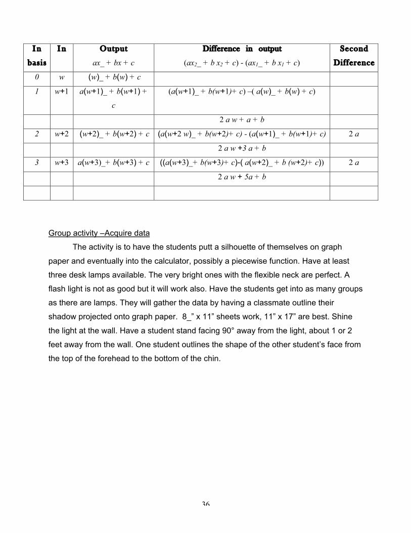
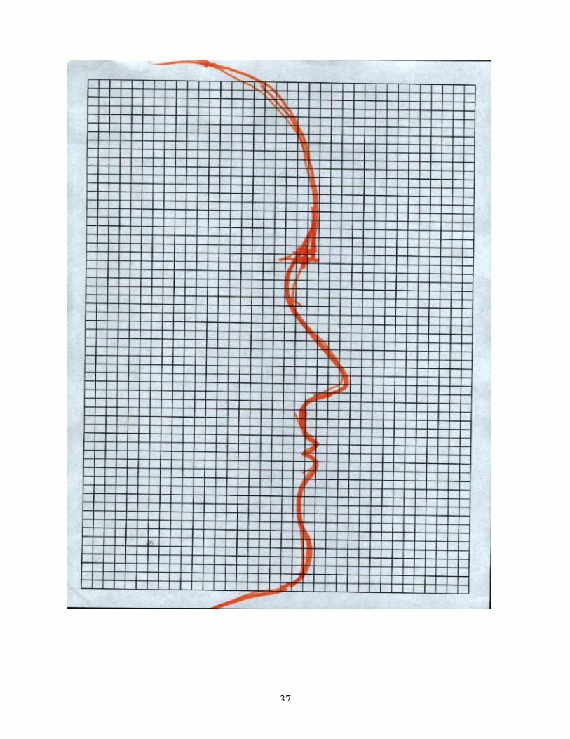
Group activity –Acquire data

The activity is to have the students putt a silhouette of themselves on graph

paper and eventually into the calculator, possibly a piecewise function. Have at least

three desk lamps available. The very bright ones with the flexible neck are perfect. A

flash light is not as good but it will work also. Have the students get into as many groups

as there are lamps. They will gather the data by having a classmate outline their

shadow projected onto graph paper. 8_” x 11” sheets work, 11” x 17” are best. Shine

the light at the wall. Have a student stand facing 90° away from the light, about 1 or 2

feet away from the wall. One student outlines the shape of the other student’s face from

the top of the forehead to the bottom of the chin.

37

38

Some questions while they are working.

Could this be a function? Why or Why not?

[Infuse vertical line test notion. Try to get the definition of function into the

conversations.]

If we had a formula for this, what family might it fit into? What gave you the hint that a

certain family would work?

[Get students to recite attributes of families and discuss them.

Get them to realist that if they turn the silhouette with the face facing up then it could

probably qualify as a function.

Could we graph it? Why? Why not? [Students should realize that this complex shape

does not fit one of our models]

Solicit any suggestions [try to get students to realize that we can graph this with plotting

points]

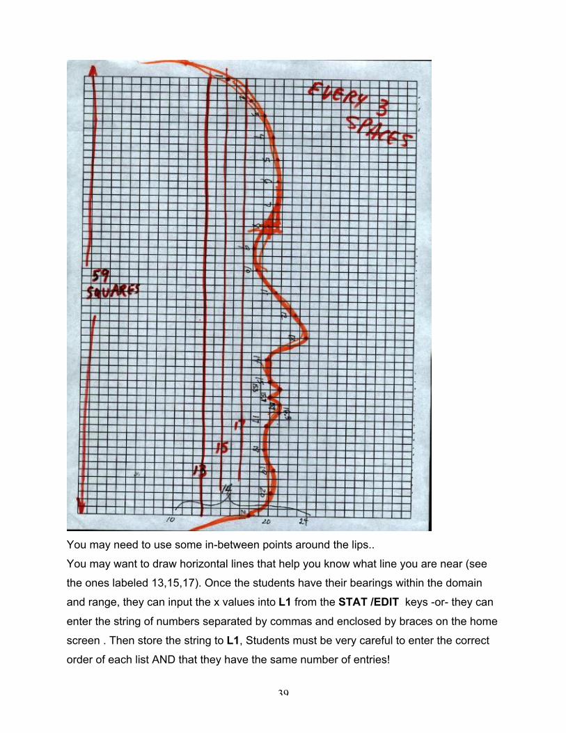
How can we decide the scale of our axis? [It does not really, although it will be easier if

we keep the input numbers separated by equal increments. I counted the amount of

squares in the height of my head’s shadow and I divided roughly to get 20 points

Have the students start thinking about scaling their range and domain. Get them to use

math terminology about their situation. My student’s picture spanned 59 squares by 24.

Therefore, this student should pick one spot on the silhouette for every three columns. (I

say “columns” because we will plot the curves with the height of the head on the x-axis.)

I might suggest narrowing the graphable area of the head for the range and try to put

every point of intersection on a solid vertical line and try to set the horizontal position on

a solid line or halfway between one. Whole numbers or decimals ending in. 0 or .5 will

make it easier to graph.

39

You may need to use some in-between points around the lips..

You may want to draw horizontal lines that help you know what line you are near (see

the ones labeled 13,15,17). Once the students have their bearings within the domain

and range, they can input the x values into L1 from the STAT /EDIT keys -or- they can

enter the string of numbers separated by commas and enclosed by braces on the home

screen . Then store the string to L1, Students must be very careful to enter the correct

order of each list AND that they have the same number of entries!

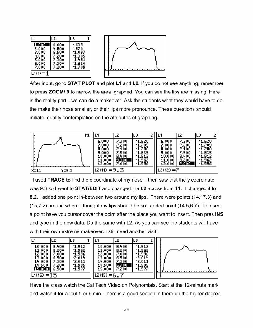
40

After input, go to STAT PLOT and plot L1 and L2. If you do not see anything, remember

to press ZOOM/ 9 to narrow the area graphed. You can see the lips are missing. Here

is the reality part…we can do a makeover. Ask the students what they would have to do

the make their nose smaller, or their lips more pronounce. These questions should

initiate quality contemplation on the attributes of graphing.

I used TRACE to find the x coordinate of my nose. I then saw that the y coordinate

was 9.3 so I went to STAT/EDIT and changed the L2 across from 11. I changed it to

8.2. I added one point in-between two around my lips. There were points (14,17.3) and

(15,7.2) around where I thought my lips should be so I added point (14.5,6.7). To insert

a point have you cursor cover the point after the place you want to insert. Then pres INS

and type in the new data. Do the same with L2. As you can see the students will have

with their own extreme makeover. I still need another visit!

Have the class watch the Cal Tech Video on Polynomials. Start at the 12-minute mark

and watch it for about 5 or 6 min. There is a good section in there on the higher degree

41

polynomial graphs. It is too long for the class but watch the section on higher degree

polynomials. Then ask the class to define what parts of their silhouette would be fit well

with a cubic, or quartic. See if they know how many relative maximums or relative

minimums (bumps) that a polynomial has. If their calculator had an unlimited degree of

regression ability, what would they set it on to get their whole silhouette in one function?

[The answer: The polynomial degree would be one more than the number of points of

inflection in the curve, or bumps] . It is fun to separate the sections of the curve into

sectors that can be regressed quit closely, then accumulate the multiple representations

to give the final single result

Homework

Assignment: p. 275 in the text

42

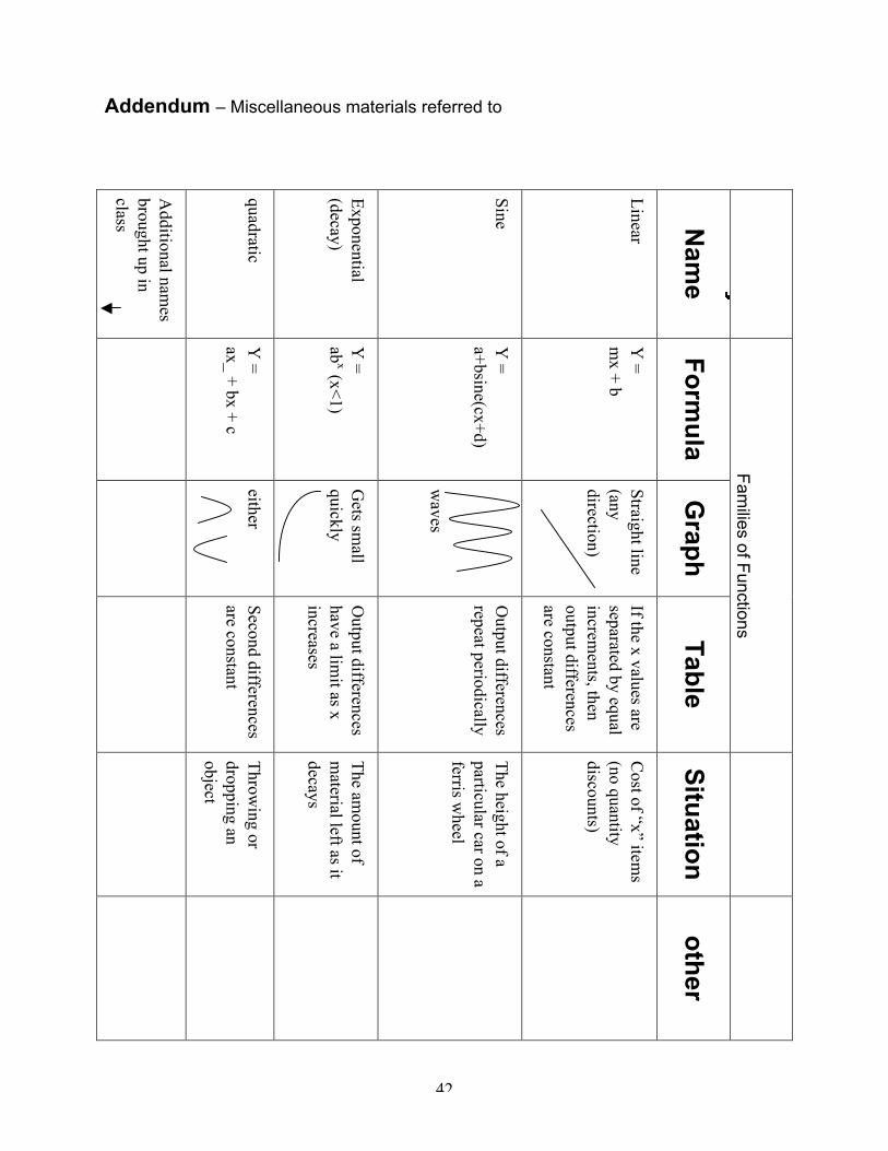
Addendum – Miscellaneous materials referred to

Additional nam

esbrought up inclass

quadratic

Exponential

(decay)

Sine

Linear N

ame

Y =

ax_ + bx + c

Y =

abx (x<1)

Y =

a+bsine(cx+d)

Y =

mx + b

Fo

rmu

la

either

Gets sm

allquickly

waves

Straight line(anydirection)

Grap

h

Second differencesare constant

Output differences

have a limit as x

increases

Output differences

repeat periodically

If the x values areseparated by equalincrem

ents, thenoutput differencesare constant

Tab

le

Fam

ilies of Functions

Throw

ing ordropping anobject

The am

ount ofm

aterial left as itdecays

The height of a

particular car on aferris w

heel

Cost of “x” item

s(no quantitydiscounts)

Situ

ation

oth

er

43

For transparency on Day 5

325°

Curved or abruptchange isacceptable

x

t

Room temp.

If oven is turned off, itcools down to room temp.

If oven is not turned off, itstays at 325°Time

Temperature

DayI I

Day II and IV

44

Chart for class work Day III

fa

hc

g

45

In(x)

Out(x_+ 3x – 2)

Differencein outputs

Seconddifference

3

4

5

6

7

Chart for class work Day III

46

In(x)

Out(x_+ 3x – 2)

Differencein Outputs

SecondDifference

3

4

5

6

7

47

Homework Day III

A. In the text (p.269-270: #1, 3) this will be handed in as a quiz grade.

B. Record your guesses. Are the two activities we did in class going to be linear,

quadratic, or neither? Give a brief reason why you have your opinion.

______________________________________________________________________

_____________________________________________________________________

______________________________________________________________________

_____________________________________________________________________

C. Draw the next two algebra tile figures for the expression 2x_ + 5x + 2. Record

the output differences.

2x+1

X+2

((x+1)+2)(x + 3)

2(x+1)+12x + 3

48

In(TIME) Out(DISTANCE) Difference in Outputs(the out value in this rowminus the out value in the next row.)

Second Difference

0 1.66213 0.043008 1.37925 0.086016 0.9734 0.129024 0.50404 0.172032 0

0.21504 0.45404 0.258048 0.84548 0.301056 1.17836 0.344064 1.45223 0.387072 1.66393

0.43008 1.66168 0.473088 0.06621 0.516096 0.05225 0.559104 0.05495 0.602112 0.0545

0.64512 1.66889 0.688128 1.5261 0.731136 1.2743 0.774144 0.96259 0.817152 0.58197

0.86016 0.17387 0.903168 0.28513 0.946176 0.64548 0.989182 0.93692 1.032182 1.16529 1.075182 1.33646 1.118182 1.43601 1.161182 1.47295 1.204182 1.43511 1.247182 0.13108 1.290182 0.14504 1.333182 0.1509 1.376182 0.16306 1.419182 0.15225 1.462182 0.16306 1.505182 0.14954 1.548182 0.14684 1.591182 0.1563 1.634182 0.1563 1.677182 0.16891 1.720182 0.17071 1.763182 0.17297 1.806182 0.18153 1.849182 0.16936